multidimensional mri of cardiac motion

Linkoping Studies in Science and Technology

Thesis No. 1262

Multidimensional MRI of Cardiac

Motion

Acquisition, Reconstruction and Visualization

Andreas Sigfridsson

LIU-TEK-LIC-2006:43

Department of Biomedical EngineeringDepartment of Medicine and Care

Linkoping University, SE-581 85 Linkoping, Sweden

Linkoping, June 2006

Cover:Left ventricular volume measured for all combinations

of cardiac and respiratory phases (from Paper II).

Multidimensional MRI of Cardiac MotionAcquisition, Reconstruction and Visualization

c© 2006 Andreas Sigfridsson

Department of Biomedical EngineeringDepartment of Medicine and Care

Linkoping UniversitySE-581 85 Linkoping

Sweden

ISBN 91-85523-37-2 ISSN 0280-7971

Printed by LiU-Tryck, Sweden

Abstract

Methods for measuring deformation and motion of the human heart in-vivoare crucial in the assessment of cardiac function. Applications ranging frombasic physiological research, through early detection of disease to follow-upstudies, all benefit from improved methods of measuring the dynamics ofthe heart. This thesis presents new methods for acquisition, reconstructionand visualization of cardiac motion and deformation, based on magneticresonance imaging.

Local heart wall deformation can be quantified in a strain rate ten-sor field. This tensor field describes the local deformation excluding rigidbody translation and rotation. The drawback of studying this tensor-valuedquantity, as opposed to a velocity vector field, is the high dimensionalityof the tensor. The problem of visualizing the tensor field is approached bycombining a local visualization that displays all degrees of freedom for asingle tensor with an overview visualization using a scalar field representa-tion of the complete tensor field. The scalar field is obtained by iteratedadaptive filtering of a noise field.

Several methods for synchronizing the magnetic resonance imaging ac-quisition to the heart beat have previously been used to resolve individualheart phases from multiple cardiac cycles. In the present work, one of thesetechniques is extended to resolve two temporal dimensions simultaneously,the cardiac cycle and the respiratory cycle. This is combined with volu-metric imaging to produce a five-dimensional data set. Furthermore, theacquisition order is optimized in order to reduce eddy current artifacts.

The five-dimensional acquisition either requires very long scan times orcan only provide low spatiotemporal resolution. A method that exploitsthe variation in temporal bandwidth over the imaging volume, k-t BLAST,is described and extended to two simultaneous temporal dimensions. Thenew method, k-t2 BLAST, allows simultaneous reduction of scan time andimprovement of spatial resolution.

Acknowledgments

I would like to thank my supervisors, Hans Knutsson, Lars Wigstrom andJohn-Peder Escobar Kvitting. Hans provided me with a constant stream ofideas and broadened my vision. Lars introduced me to this field and taughtme everything about magnetic resonance imaging. John-Peder guided mein understanding the function of the heart. Thank you for believing in meand giving me the encouragement I needed.

I would also like to thank my colleagues at the divisions of clinical phys-iology and medical informatics, the MRI unit and the Center for MedicalImage science and Visualization (CMIV). You provided me with the at-mosphere that I love and the opportunities for interesting discussions ona wide flora of topics. Thank you Tino, Einar, Jan, Ann, Eva, Carljohan,Per, Henrik, Petter, Marcel, Frida, Peter, Olof, Mattias, Johanna, Anders,Andreas, Bjorn, Joakim, Mats, Magnus, Pernilla, Katarina and Matts.

I would also like to take this opportunity to express my gratitude to thelate Bengt Wranne for providing this environment and opportunity for meand many of my colleagues.

This work has been conducted in collaboration with the Center for Medical Image

Science and Visualization (CMIV, http://www.cmiv.liu.se/) at Linkoping Univer-

sity, Sweden. CMIV is acknowledged for provision of financial support and ac-

cess to leading edge research infrastructure. This work was further funded by the

Swedish Research Council, the Heart Lung Foundation and the Linkoping Heart

foundation.

Contents

Abstract iii

Acknowledgments v

1 Introduction 1

1.1 Outline of the thesis . . . . . . . . . . . . . . . . . . . . . . 2

1.2 Glossary of terms and abbreviations . . . . . . . . . . . . . 3

2 Cardiac motion 5

2.1 The cardiac cycle . . . . . . . . . . . . . . . . . . . . . . . . 5

2.2 The respiratory cycle . . . . . . . . . . . . . . . . . . . . . . 6

2.2.1 Interventricular coupling . . . . . . . . . . . . . . . . 7

2.3 Myocardial deformation . . . . . . . . . . . . . . . . . . . . 8

3 Cardiac Magnetic Resonance Imaging 13

3.1 MRI Principles . . . . . . . . . . . . . . . . . . . . . . . . . 13

3.2 k -space . . . . . . . . . . . . . . . . . . . . . . . . . . . . . 13

3.3 k-t sampling . . . . . . . . . . . . . . . . . . . . . . . . . . . 15

3.4 Temporal resolution . . . . . . . . . . . . . . . . . . . . . . 15

3.4.1 Prospective cardiac gating . . . . . . . . . . . . . . . 16

3.4.2 Retrospective cardiac gating . . . . . . . . . . . . . . 18

3.4.3 TRIADS . . . . . . . . . . . . . . . . . . . . . . . . 18

3.4.4 Simultaneous resolution of both cardiac and respira-tory cycles . . . . . . . . . . . . . . . . . . . . . . . 19

3.5 k -space acquisition order . . . . . . . . . . . . . . . . . . . . 21

4 Rapid acquisition 23

4.1 k-t BLAST . . . . . . . . . . . . . . . . . . . . . . . . . . . 26

4.1.1 The x-f space . . . . . . . . . . . . . . . . . . . . . . 26

4.1.2 Fast estimation of signal distribution in x-f space . . 28

4.1.3 The k-t BLAST reconstruction filter . . . . . . . . . 30

viii Contents

4.1.4 Implementation details . . . . . . . . . . . . . . . . . 31

5 Tensor field visualization 33

5.1 Glyph visualization . . . . . . . . . . . . . . . . . . . . . . . 335.2 Noise field filtering . . . . . . . . . . . . . . . . . . . . . . . 34

5.2.1 Enhancement . . . . . . . . . . . . . . . . . . . . . . 35

6 Summary of papers 39

6.1 Paper I: Tensor Field Visualisation using Adaptive Filteringof Noise Fields combined with Glyph Rendering . . . . . . . 39

6.2 Paper II: Five-dimensional MRI Incorporating SimultaneousResolution of Cardiac and Respiratory Phases for VolumetricImaging . . . . . . . . . . . . . . . . . . . . . . . . . . . . . 39

6.3 Paper III: k-t2 BLAST: Exploiting Spatiotemporal Structurein Simultaneously Cardiac and Respiratory Time-resolvedVolumetric Imaging . . . . . . . . . . . . . . . . . . . . . . 40

7 Discussion 41

7.1 Multidimensional imaging . . . . . . . . . . . . . . . . . . . 417.2 Using k-t2 BLAST for respiratory gating . . . . . . . . . . . 427.3 Costs of sparse sampling . . . . . . . . . . . . . . . . . . . . 42

7.3.1 Noise . . . . . . . . . . . . . . . . . . . . . . . . . . 437.3.2 Temporal fidelity . . . . . . . . . . . . . . . . . . . . 43

7.4 Future work . . . . . . . . . . . . . . . . . . . . . . . . . . . 447.4.1 Validation . . . . . . . . . . . . . . . . . . . . . . . . 447.4.2 Tensor field data quality . . . . . . . . . . . . . . . . 457.4.3 Optimizing reduction factor versus temporal fidelity 457.4.4 Acquisition of velocity data using k-t2 BLAST . . . 45

7.5 Potential impact . . . . . . . . . . . . . . . . . . . . . . . . 45

Bibliography 47

Chapter 1

Introduction

Cardiovascular disease is the leading cause of death in the western world.In Sweden, diseases of the circulatory system was the cause of death of45% of the men and 44% of the women who died in 2003 [1]. Of thesedeaths, ischemic heart disease was the largest group, accounting for 23%of male deaths and 18% of female deaths. Decades of research has beenconducted to understand the function of the healthy heart, the changesassociated with disease, and the causes thereof. Functional studies of theheart wall are the cornerstone for the assessment and follow-up of a largerange of cardiac diseases. Cardiac motion and deformation are fundamentalproperties that are of interest to comprehend the impact of diseases oncardiac function. Quantification of motion and deformation would lead toless subjective assessment and improve our ability to compare the effect ofdifferent treatment strategies.

The aim of this thesis was to develop methods for measuring deforma-tion and motion of the heart in-vivo with the use of magnetic resonanceimaging (MRI).

To fulfill this goal, the following approaches were investigated:

• Visualization of the local heart wall deformation. This involves com-puting a strain rate tensor field from a volumetric velocity measure-ment of the heart. The strain rate tensor is insensitive to regionaltranslation but instead describes the rate of local lengthening or short-ening. The tensor field is visualized using a combination of traditionalglyph rendering of a single tensor with tensor-guided adaptive filter-ing of noise fields for overview visualization.

• Acquisition of volumetric images resolved over both cardiac and respi-ratory cycles simultaneously. This produces a five-dimensional data

2 Introduction

set, allowing for example measurement of interventricular couplingduring the respiratory cycle. This is accomplished by combining afast MRI pulse sequence with a triggering method extended to two si-multaneous temporal dimensions. The acquisition order is optimizedto minimize artifacts in the images.

• Acquisition time reduction by sampling data sparsely and exploitingspatiotemporal correlations during reconstruction. With this tech-nique, the long acquisition time for five-dimensional imaging can becut in half while spatial resolution is simultaneously quadrupled. Thesparse sampling enables sharing temporal bandwidth between staticand dynamic parts of the imaging volume, allowing for a significantlymore efficient use of scan time.

1.1 Outline of the thesis

This thesis is organized as follows. In Chapter 2, a brief overview of motionof the heart during the cardiac and respiratory cycles is provided. Further-more, the strain rate tensor, describing the local heart wall deformation, isintroduced. Principles of cardiac MRI and temporally resolving samplingprocedures in particular are presented in Chapter 3. In Chapter 4, ways toshorten acquisition time are discussed, mainly focused on the k-t BLASTmethod. Visualization of the heart wall deformation strain rate tensor fieldis described in Chapter 5. Chapter 6 contains short summaries of the papersthat are part of this thesis, and Chapter 7 contains discussion.

1.2 Glossary of terms and abbreviations 3

1.2 Glossary of terms and abbreviations

Aliasing The replication of a signal caused by periodic sam-pling. The aliased signal appears at different posi-tions in the corresponding transform space, e.g. atdifferent spatial positions, spatial frequencies, tem-poral positions or temporal frequencies.

ECG ElectrocardiogramFOV Field of viewIn-vivo Within a living organism, as opposed to in-vitro (in

the laboratory).k -space The spatial frequency domain of the object being

imaged in magnetic resonance imaging.k-t BLAST k-t Broad-use Linear Acquisition Speed-up Tech-

nique. A method to reduce acquisition time bysparse sampling in k-t space, with subsequent aliassuppression during reconstruction.

LIC Line integral convolution, a vector field visualizationtechnique.

M-mode Motion mode. Display of dynamics by presenting thetemporal dimension on a spatial axis, widely used inultrasound.

MRI Magnetic resonance imagingMyocardium Heart muscleSSFP Steady State Free Precession. An MRI pulse se-

quence widely used for cardiac imaging.TRIADS Time-Resolved Imaging with Automatic Data Seg-

mentation. A method for resolving motion withautomatic division of the cycle into multiple timeframes.

Voxel Volume element

4 Introduction

Chapter 2

Cardiac motion

There are several types, or scales, of cardiac motion that are meaningful tostudy. Deformation or strain in the cardiac muscle can give useful infor-mation about the local function of the muscle. Wall thickening and motioncan also give important regional information. The interaction between theleft and right ventricles is a more global effect that is influenced by pressuredifferences external to the heart, such as caused by respiration.

2.1 The cardiac cycle

The heart is the organ responsible for pumping blood throughout the body.It is divided into four chambers; the left and right atria and the left andright ventricles, as shown in Figure 2.1. The pump function of the heart isperiodic, and the cardiac cycle is divided into two main phases, diastole andsystole. In the diastolic phase, the left and right ventricles are filled withblood from the atria through the mitral and tricuspid valves. In the systolicphase, the ventricles contract and blood is ejected through the aortic andpulmonary valves to the aorta and the pulmonary artery.

Both the left and right sides of the heart beat approximately simulta-neously. The two sides are connected in series with the systemic circuitthrough the body and the pulmonary circuit through the lungs. Deoxy-genated blood from the body is delivered to the right atrium. The bloodfills the right ventricle and is subsequently ejected through the pulmonaryartery and into the lungs, where it is oxygenated. Oxygenated blood isdelivered to the left atrium which then fills the left ventricle. The left ven-tricle ejects the oxygenated blood through the aortic valve to the aorta,which is connected to the rest of the body.

Common heart rates in healthy persons are 45–80 beats per minute.

6 Cardiac motion

a b

RA

LA

LV

RV

Figure 2.1: Cardiac configuration in systole (a) and diastole (b) in a four-chamber view. The arrows indicate the right ventricle (RV), right atrium(RA), left ventricle (LV) and left atrium (LA).

The duration of the systolic phase usually varies very little with changingheart rates, but the duration of the diastolic phase can vary substantially.The thickness of the myocardium, the heart wall, of the left ventricle rangesfrom around 10 mm at the end of diastole to 15 mm at the end of systole.The right ventricular walls are significantly thinner, measuring 5.3 mm and5.6 mm in end diastole and end systole, respectively. The outer contoursof the heart are surprisingly static during the cardiac cycle, as shown inFigure 2.1. Substantial contribution to the volume changes is made byshifting the atrio-ventricular plane in the apex to base direction with thevalves open during diastole and in the opposite direction with the valvesclosed during systole [2].

What is commonly measured to assess cardiac motion is wall thicknessvariations during systole and diastole. Synchrony of the different parts ofthe ventricle can also be of interest, especially when studying effects ofmyocardial ischemia and infarction [3].

2.2 The respiratory cycle

Cardiac motion is highly affected by respiration. The most dominant ef-fect of respiration is the effect on heart position. During inspiration, thediaphragm, a muscular interface between the abdominal and thoracic cavi-ties, pulls downward, allowing the lungs to expand. The heart is attached tothe diaphragm, and is being pulled down during inspiration. Chest muscles

2.2 The respiratory cycle 7

also expand the chest cage, but to a much lesser extent than the expansioncaused by the diaphragm. This is illustrated in Figure 2.2.

ba

Figure 2.2: Cardiac positions in end expiration (a) and end inspiration (b).The heart is shifted as the diaphragm is pulled down during inspiration.

Respiration also affects the pressure in the thorax. During inspiration,pressure is lowered, to force air from the outside into the lungs. Thislowering of pressure reduces resistance in the vena cavas, the veins thattransport deoxygenated blood from the body into the right atrium. This inturn increases filling of the right ventricle. At the same time, resistance inthe pulmonary system is increased, reducing the filling of the left ventricle.During expiration, the pressure and the corresponding effects are reversed.

Typical respiratory rates vary between 10–20 cycles per minute. Theheart can be shifted as much as 12 mm. The effects of respiration is moreindividual than that of the cardiac cycle.

2.2.1 Interventricular coupling

With changing pressures in the thorax, filling of the ventricles is affecteddifferently in the left and right sides. This results in changing volumes andpressures between the ventricles. The interventricular septum regulatesthis, shifting from one side to the other, in order to allow for volume orpressure increase. This shift has been demonstrated by the method pre-sented in Paper II and is shown in Figure 2.3. This is referred to as couplingbetween the ventricles, and is important in several diseases. Some diseasesaffect the pericardium surrounding the heart. A stiffer pericardium will ex-aggerate the interventricular coupling. The ventricular coupling is presenteven without any pericardium, but the effect is reduced [4]. Acute changesin left ventricular function due to abrupt pressure overload of the right ven-tricle (e.g., from pulmonary embolism) may be explained by interventricularcoupling. Long-term right ventricular volume overload, for example causedby pulmonary valve insufficiency, can also be linked to the interventricular

8 Cardiac motion

PSfrag replacements

RFW

[mm

]RS

[mm

]LS

[mm

]LF

W[m

m]

RVdi

amet

er[m

m]

LVdi

amet

er[m

m]

Expiration Inspiration






51

52

53

54

55

30

30.5

31

31.5

32

32.5

33343536

84

86

88

96

97

98

127

128

129

Figure 2.3: Septal motion over the cardiac cycle, presented in Paper II. Thewall positions of the inner right ventricular free wall (RFW), right side of theseptal wall (RS), left side of the septal wall (LS) and inner left ventricularfree wall (LWF) were traced through the respiratory cycle in an end diastoliccardiac phase and shown on the left. Note that the septal wall moves towardsthe right ventricle during expiration and towards the left ventricle duringinspiration. On the right, the computed right ventricular (RV) diameter andleft ventricular (LV) diameter show RV diameter decreasing during expirationand increasing during inspiration. LV diameter demonstrates the oppositebehavior.

interdependence [5]. After open heart surgery, abnormal septal wall motionis commonly observed [6]. The pathophysiological mechanism behind thisphenomenon is still disputed [7, 8].

2.3 Myocardial deformation

Local deformation of the myocardium is an important measure of its func-tion. In the deformation estimate, translation is usually excluded, providingonly a measure of local lengthening and shortening. Damaged muscle tis-sue is expected to produce less deformation, but it may still show large

2.3 Myocardial deformation 9

Figure 2.4: Illustration of the stress tensor acting on a point. The tensorcomponents are the stresses acting on different cut planes.

translation, due to pulling or pushing by neighboring healthy tissue [2].

Deformation and stress of a small volume is usually quantified using atensor. The general definition of a tensor involves a vector space V and itsdual. We will only be interested in the case where V is equipped with afixed scalar product, in which case the definition of a tensor is a multilinearmapping from a number of vector spaces (V ) onto the real space (R). Therank of a tensor is the number of arguments to the mapping. Scalars andvectors are special cases of tensors, namely tensors with ranks 0 and 1,respectively. We will consider the special case of tensors with rank 2. Inthis case, the tensor is a bilinear mapping V × V → R. There is a one-to-one correspondence of these tensors with mappings V → V . The tensor isthen naturally identified with this latter mapping.

Internal forces acting on a body can be described by the stress tensor.One may think in terms of virtually cutting the body along a cut plane.There is a force acting upon this cut plane, not necessarily perpendicularto the plane, but generally having components of shear orthogonal to theplane normal. This is illustrated in Figure 2.4. The stresses acting on threeorthogonal cut planes are shown on the surfaces of a box. The stresses canbe of arbitrary direction, as illustrated by the decomposition into three or-thogonal components, one in the normal direction, representing the normalstress, and two in the surface plane, representing shear stress. Since thetensor is linear, the stress vectors need only to be obtained for three linearlyindependent cut planes in order to determine the tensor completely.

The stress tensor is the linear mapping from the cut plane, which may berepresented by its normal vector, to the stress vector. The correspondencewith the mapping V ×V → R is then how much stress on a cut plane (first

10 Cardiac motion

Figure 2.5: Eigen decomposition of the deformation of a square. The dottedsquare is the original state and the stippled parallelogram is the deformedstate. The arrow on the square indicates shear force. The eigen decompositionis illustrated to the right, with a large lengthening in one diagonal directionand a somewhat smaller shortening in the other diagonal direction.

argument) there is along a probe vector (second argument).

Eigen decomposition is useful to aid interpretation, after which three (inthree dimensions) eigenvectors and corresponding eigenvalues are obtained.The eigen decomposition is easiest considered when viewing the tensor asthe mapping V → V and representing the cut plane with its normal vector.An eigenvector e to a mapping T is a vector which is mapped to itselfscaled by the eigenvalue λ, i.e. Te = λe with e ∈ V . In other words,the eigenvector is the normal to a cut plane containing only normal stressand no shear stress. An example of eigen decomposition is illustrated inFigure 2.5

Common notation for the stress tensor components is a 3 × 3 matrix.The Cauchy stress tensor is symmetric [9], so the matrix representation isalso symmetric. This means that the eigenvalues are real and the eigenvec-tors are orthogonal.

With the stress tensor representing stress, force per unit area, there isa corresponding strain tensor, representing local normalized deformation.The strain tensor is related to the stress tensor through a constitutivelaw. Strain reflects the shape change between two states, one state usu-ally being some kind of reference state. This usually requires tracking ofpoints through time, not readily available with non-invasive methods suchas MRI. Tagging [10] or point tracking in velocity fields [11] can providedata suitable for estimating myocardial strain, but limitations in spatialresolution makes this approach difficult. Another way to characterize my-ocardial deformation is to directly measure velocity by using phase contrastMRI [12, 13]. From the measured velocity field, a spatial derivative, the

2.3 Myocardial deformation 11

Jacobian L, can be computed according to

L = ∇v =dv

dx∼

∂v1

∂x1

∂v1

∂x2

∂v1

∂x3

∂v2

∂x1

∂v2

∂x2

∂v2

∂x3

∂v3

∂x1

∂v3

∂x2

∂v3

∂x3

(2.1)

where ∼ denotes component representation, v ∼ (v1 v2 v3)T is the velocity

vector and x ∼ (x1 x2 x3)T are the spatial coordinates. The asymmetric

part of the Jacobian represents the rigid body rotation, while the symmetricpart is called the strain rate tensor. The Jacobian is symmetrized accordingto

D =1

2(L + LT ) (2.2)

This tensor represents the instantaneous rate of change of strain andhas the physical unit s−1. The strain rate tensor is commonly used in fluidstudies, but may also be applied to studies of myocardial mechanics.

By studying the strain rate instead of the velocity, information is notcontaminated by translation possibly caused by adjacent muscle contractionand relaxation. The price for this convenience is the necessity to study thehigher dimensional quantity of the tensor instead of the much simpler vectorvalued velocity. This can be alleviated to some extent by performing eigendecomposition of the tensor. The directions of the eigenvectors representthe principal directions of lengthening or shortening. In the case of thestrain rate tensor, the eigenvalue then represents the rate of lengthening(positive) or shortening (negative).

12 Cardiac motion

Chapter 3

Cardiac Magnetic Resonance

Imaging

3.1 MRI Principles

MRI is an imaging modality that exploits the nuclear magnetic resonancephenomenon, and is commonly used to produce images of the hydrogenproton distribution in humans. Hydrogen is abundant in the human bodyin the form of water molecules. MRI incorporates a strong external homo-geneous magnetic field, which is used to align the spin distribution of thehydrogen protons along the magnetic field direction. A rotating magneticfield, usually referred to as radio frequency field, is then applied. Tunedto the Larmor frequency of the spins, it is used to tip the spin distributionaway from the main magnetic field direction. This tipping is referred toas excitation. After the excitation, the spin distribution undergoes a re-laxation process, in which the distribution returns to be directed along themain magnetic field. During this relaxation, the spins emit a signal thatis received using induction in coils. During signal reception, additionalspatially varying magnetic fields, referred to as the gradients, are appliedto encode the spatial position of the signal. The combination of gradientwaveforms and rotating magnetic field pulses is called a pulse sequence.

3.2 k-space

In MRI, data is naturally acquired in the Fourier domain, which is calledk -space. During readout of the MRI signal, which is usually seen as acomplex-valued signal, the spatially varying gradients encode a linear phaseon the imaging object. A gradient with strength G applied during a time

14 Cardiac Magnetic Resonance Imaging

period of t modulates the signal at a location x according to

eixγR

t

0G(τ)dτ (3.1)

where γ is the gyromagnetic ratio of the hydrogen proton. Combined withthe fact that the signal is received from the whole object simultaneouslyand the substitution k = γ

2π

∫ t

0 G(τ)dτ , the signal S follows a familiarrelationship, a Fourier transform:

S =

∫

X

ρ(x)eix2πkdx (3.2)

where the integral is performed over all spatial positions and ρ is the protondensity. This is a highly simplified model, disregarding relaxation, signaldecay and spatially varying coil sensitivity during reception, among otherthings. Nevertheless, it illustrates the Fourier encoding and the role ofk -space as the spatial frequency domain.

The waveforms of the gradients are chosen in order to collect data fromdifferent parts of k -space. The sequence of excitation and signal receptionduring gradient application is repeated many times to collect signal fromsufficient parts of k -space to be able to reconstruct an image of the object.Each repetition uses a different gradient strength for the spatial encoding,to sample different points in k -space. The gradients can be applied in anyspatial direction, making it possible to acquire three-dimensional images. Aspecial case is the so-called “read-out” or “frequency encoding” direction.The gradient in this direction is commonly applied constantly during thesignal reception, making a sweep through k -space in this direction while thesignal is sampled at a high sampling frequency. This is the measurementof a k -space line, sometimes referred to as a k -space profile.

For objects with sharp details, high spatial frequencies need to be sam-pled. This requires sampling of a larger area of k -space using several rep-etitions and, consequently, a longer acquisition time. Since the spatialfrequency domain is being sampled instead of the normal spatial domain,function domain and transform domain can be seen as reversed when com-pared to conventional signal processing of temporally or spatially sampledsignals. Concepts of sampling density and Nyquist aliasing etc. show upin new places. Since humans have a finite spatial extent, the sampled sig-nal is guaranteed to be band limited. This translates into a requirementfor the sampling density in k -space to be able to reconstruct the objectwithout aliasing. If k -space is not sampled densely enough, spatial alias-ing will occur. This is because regular sampling in the function domain(k -space) will cause periodic repetition of the signal in the reciprocal trans-

3.3 k-t sampling 15

form domain (the spatial domain). The sampling can be represented as amultiplication by the shah-function, III(k), defined as1

III(k) =

inf∑

n=−inf

δ(k − n) (3.3)

with δ as the Dirac impulse. The convolution theorem states that multipli-cation of two signals in the function domain corresponds to convolution oftheir transforms in the transform domain. Since III(k) is self-reciprocal [14],i.e. it is its own Fourier transform, this means that the transform of thesampled signal is replicated, or aliased, periodically. Furthermore, the simi-larity theorem states that if a function f(x) has the Fourier transform F (s),then the Fourier transform of f(ax) is 1

|a|F ( sa). This means that the aliased

signals get closer to each other with larger sampling distance. If the aliasedsignals overlap, the true signal can no longer be recovered correctly.

3.3 k-t sampling

In dynamic imaging, k -space must be sampled over time as well. Time isdiscretized in a number of time frames with sufficient rate to capture thedynamics of the object being imaged. The standard method is to sampleeach k -space position once in every time frame. This can be referred toas regular sampling of the k-t space with full density, shown in Figure 3.1together with the resulting aliasing of the signal in the x-f space.

To reconstruct the data sampled with full density as above, a rectanglefunction can be used to cut out the transform of the main signal. If data isnot fully sampled, or equivalently, if the transform is larger than expected,the aliased signals will overlap with the main signal transform, causingreconstruction errors, as shown in Figures 3.2. This is actually quite oftenthe case, especially in the temporal dimension, because the object beingimaged is seldom truly bandlimited in the temporal dimension. This is nota big problem, because the energy content in the high temporal frequencycomponents is very small compared to in the lower frequency components.

3.4 Temporal resolution

Requirements for spatial and temporal resolution for cardiac imaging oftenrequire acquiring data over the course of several heart beats. By assuming

1The shah-function is usually defined as a function of x, but since sampling in MRI

is performed in k -space, the argument variable k is used here.


k x

t f

Figure 3.1: Regular k-t sampling with full density. Each dot shows a sam-pling position (left) and the corresponding transforms of the signal (right,white) and aliased signal (right, gray) are separated enough, enabling alias-free reconstruction.

that the object undergoes identical motion in each heart beat, differentparts of k -space can be sampled in the same cardiac phase but in differ-ent cardiac cycles. This is a quite good approximation, but degraded byrespiration or arrhythmia during the acquisition.

There are different methods of controlling k -space acquisition order andkeeping track of which parts of k -space have been acquired during theexperiment.

3.4.1 Prospective cardiac gating

Prospective cardiac gating [15], sometimes called triggering, works by al-ternating monitoring of a cardiac triggering device, such as an electrocar-diogram (ECG), and acquisition of k -space data. The acquisition schemestarts by waiting for an R-peak in the ECG, meaning the onset of systole.After the R-peak is detected, the acquisition is delayed for a predeterminedtime, trigger delay. After the trigger delay, a fixed predetermined number oftime frames are collected by acquiring another fixed predetermined numberof k -space profiles for each time frame. After acquiring data from all timeframes, monitoring of the triggering device is repeated. In each successivecardiac cycle, different lines in k -space are acquired. The acquisition isfinished when all k -space lines have been acquired.

3.4 Temporal resolution 17

k x

t f

k x

t f

a b

dc

Figure 3.2: Regular k-t sampling with half density in the spatial frequencydimension (a) results in overlapping aliased signals (b), causing spatial aliasingerrors after reconstruction. Regular k-t sampling with half density in thetemporal dimension (c) also results in overlapping aliased signals (d), causingtemporal frequency aliasing errors after reconstruction.

In prospective methods, the time frames are classified already duringacquisition, making reconstruction easy. No interpolation is necessary andall cardiac cycles and k -space lines have the same number of time frames.

The drawback of this method is its inability to image the later parts ofthe cardiac cycle, because the number of cardiac time frames acquired needsto be fixed and set small enough to allow the scanner to start monitoringthe ECG before the next R-peak. Some variation of cardiac frequency isexpected, further limiting the number of cardiac time frames. The advan-tage is the simplicity of acquisition and reconstruction. This method isoften used when only one time frame in a specific phase of the cardiac cycleis of interest, such as coronary artery magnetic resonance angiography.


3.4.2 Retrospective cardiac gating

Retrospective cardiac gating [16], often referred to as cine imaging, solvesthe problem of imaging the whole cardiac cycle. One common approachincorporates simultaneous acquisition and monitoring of the ECG. In thesimplest form, acquisition starts by continuously measuring the first k -space line. When an R-peak is detected, acquisition is advanced to thenext k -space line. Acquisition is terminated when the whole k -space hasbeen acquired. Instead of only acquiring one k -space line continuously, onecan alternate between several, trading temporal resolution for scan time.Also, k -space order is not necessarily linear from top to bottom, but canfollow more advanced schemes.

Because of variations in heart rate, the number of measurements foreach k -space line is not the same for every k -space line. The k -space datais then usually interpolated over time to a number of evenly distributedtime frames. This interpolation usually stretches the cardiac cycle linearly,but some more advanced models have been proposed. One such modelassumes a constant length systole and stretches diastole linearly, but it hasnot shown significant improvement over the simple linear model [16].

The benefits of the retrospective method is the ability to resolve thecomplete cardiac cycle, at the expense of implementation complexity.

3.4.3 TRIADS

A method that provides a flexible trade-off between acquisition time andtemporal resolution is Time Resolved Imaging with Automatic Data Seg-mentation (TRIADS) [17]. Instead of following a fixed scheme for everycardiac cycle, acquisition is adapted to the cardiac phase. TRIADS de-cides which k -space line to acquire at a given time, in contrast to the cinemethod, which decides the time(s) to acquire a given k -space line. Forevery repetition of the TRIADS acquisition, the current cardiac phase isestimated. The estimated cardiac phase is then binned into one of a fixednumber of time frames prescribed. TRIADS keeps track of which partsof k -space have already been acquired for each individual time frame, andacquires a new k -space line. The acquisition continues until a full k -spacehas been acquired for all time frames.

In cine imaging, temporal resolution is prescribed by a fixed multiple ofthe repetition time, which leads to varying number of time frames acquiredfor each k -space line. In contrast, TRIADS prescribes a number of timeframes, and every cardiac cycle is divided into this number of time frames.Temporal resolution in milliseconds will then vary to be able to fit the

3.4 Temporal resolution 19

number of time frames into the cardiac cycle. A schematic comparisonbetween the cine method and TRIADS is shown in Figure 3.3.

yk

yk yk

yk

Acquisition stage Reconstruction stage

timeframe

timeframe

cine

TRIADS

Figure 3.3: An example of cine and TRIADS acquisition schemes. In cineimaging, the acquired profiles (ky) are changed at each R-peak. In TRIADS,cardiac phase, shown as circles with different shades in this example with fourtime frames, is estimated for each repetition. Previously acquired profiles aretracked individually for each time frame. Note that in TRIADS, the timeframes are not required to come in a predictable order.

Since the binning into time frames is done during acquisition in TRI-ADS, reconstruction is as simple as for the prospective method. Indeed,one may regard TRIADS as a prospective method, as the binning intotime frames usually involves predicting the duration of the current car-diac cycle based on previous cardiac cycles, as opposed to designating timeretrospectively. A major difference between TRIADS and prospective gat-ing is TRIADS ability to image the complete cardiac cycle. Retrospectivere-binning may be performed by interpolation, refining the cardiac phaseestimates. This requires that appropriate k -space lines have been acquiredat a reasonable number of time points spread over the cardiac cycle. Theprospective phase estimates thus still needs to be accurate to some extent.

3.4.4 Simultaneous resolution of both cardiac and respira-

tory cycles

In order to measure cardiac motion affected by respiration, the respiratorycycle needs to be resolved. Since there is still motion during the cardiaccycle, sampling must be synchronized with the cardiac cycle. This can


be accomplished by using a prospective triggering approach and acquiringonly one time frame per cardiac cycle, but this reduces scan efficiency,because time is wasted waiting for the particular period in every cardiaccycle. Better efficiency can be achieved by continuously acquiring data,resolving both cardiac and respiratory cycles simultaneously. This means,acquiring a full image or volume for every combination of cardiac phase andrespiratory phase. This adds a new dimension to cardiac imaging, beingable to freeze motion during the cardiac cycle and examine what effects therespiration induces on cardiac function.

With simultaneous resolution of both cardiac and respiratory cycles, thetime line becomes two-dimensional. If the cardiac and respiratory cyclesare fully covered, as when using the TRIADS method, both dimensions arecyclic. The topology of the temporal dimensions can then be visualizedas a torus, as shown in Figure 3.4. Even though the individual temporaldimensions are cyclic, their combination in actual time is more complex.This makes the cine and prospective methods unsuitable for acquiring dataresolved to both dimensions simultaneously. The TRIADS method, how-ever, only requires that the phases in the individual cycles can be estimated.Every repetition in the acquisition then involves estimating both cardiacand respiratory phase, classifying them into a combined time frame, andthe TRIADS scheme takes care of filling the k -space in every time frame.

PSfrag replacements

-2

-1

0

1

2

-2

0

2

-0.5

0

0.5

Cardiac time

Resp

irato

ry ti

me

Cardiac time

Respiratory time

Figure 3.4: Simultaneous resolution of both cardiac and respiratory cyclesgives a two-dimensional temporal plane (left). Since the plane is cyclic inboth dimensions, the topology can be visualized as a torus (right).

Acquisition of simultaneous resolution of cardiac and respiratory cyclesin a two-dimensional slice has been presented previously [18]. In that work,TRIADS was used to resolve the respiratory cycle, but within each cardiaccycle, retrospective cine imaging was performed. This caused the respira-tory phase estimates made at the beginning of every cardiac cycle to be

3.5 k-space acquisition order 21

assumed constant throughout that cardiac cycle. In Paper II, a volumet-ric method is presented, extending TRIADS to two simultaneous temporaldimensions.

3.5 k-space acquisition order

In cardiac imaging, balanced steady-state free precession (SSFP) [19] is afrequently used pulse sequence. It provides strong signal from the bloodand allows for short repetition times with maintained signal level. Thiscomes at the requirement of a fast gradient switching system and a stablehomogeneous magnetic field. Gradient systems that are fast enough arereadily available, but disturbances in the magnetic field can in some casesbe a problem. One cause of problem is eddy currents disrupting the steadystate. These eddy currents can be caused by large changes in phase encod-ing gradient strength between successive excitations [20], i.e. large jumpsin k -space.

These effects can be removed by acquiring the same k -space line twicein two successive excitations and taking the complex average [21]. Thiswill double acquisition time, however. A way to reduce the effects is tominimize the jumps in k -space by choosing an appropriate acquisition or-der. For prospective and retrospectively gated acquisitions, this is easy,since the k -space order can be controlled directly, and jumps can be min-imized by choosing a zig-zag pattern. In TRIADS, however, the alreadyacquired parts of k -space are generally different for different time frames.Time frames may be acquired in a non-predictable order, especially whenresolving two independent temporal dimensions. Furthermore, the time be-tween excitations is very short, imposing a limit to how much computationscan be performed in order to optimize the acquisition order in runtime. InPaper II, this is solved by using a predefined k -space profile order curveand keeping a time-frame local progress counter that indicates how manylines along this profile order curve have been acquired for that particulartime frame. The profile order curve is a discrete mapping from the one-dimensional progress counter to the two-dimensional ky − kz space. Thekx dimension is covered by reading a whole line in k -space for each rep-etition. Typically, the time spent in each time frame is on the order of10–15 excitations until the time frame is changed. Since all timeframes areapproximately equally common, the differences between progress countersis expected to be small. This imposes three design criteria on the profileorder curve:

• Each point in the ky − kz plane should be visited exactly once.


• Two subsequent points along the curve should be adjacent to eachother in ky − kz space.

• The distance in ky − kz space between two fairly close points on thecurve should be minimized.

A curve which addresses these design goals is the Hilbert curve, proposedby David Hilbert in 1891. The locality of the Hilbert curve is close tooptimal [22], meaning the maximum value of

|Hilbert(p1) − Hilbert(p2)|2

|p1 − p2|(3.4)

has a low bound. The squared distance in the numerator is computed inky − kz space and the distance in the denominator is the distance alongthe curve for two different points p1 and p2. This means that close pointsalong the curve are also close in the ky − kz space. Thus, when the timeframe differs between excitations, the jump in k-space will be kept short. Afirst order Hilbert curve consists of a single U-shape as seen in Figure 3.5a.Subsequent levels are generated by replacing the U-shape with four rotatedversions linked together with three joints (Figure 3.5b-d).

PSfrag replacements123450

0.51

c da b

Figure 3.5: A Hilbert plane filling curve can be used to control acquisi-tion order to reduce eddy current effects in balanced SSFP imaging. It isconstructed recursively, and levels 1 through 4 are shown in a-d.

Chapter 4

Rapid acquisition

The demands for spatial and temporal resolution in cardiac MRI are usuallynot compatible with the desired acquisition time. Spatial resolution maybe improved by acquiring more of k -space, at the expense of increased scantime and decreased signal-to-noise. Scan time may be reduced by decreas-ing temporal resolution, which is often not desirable. Increase of temporalresolution is also usually limited by the shortest repetition time available.Much effort has been put into reducing scan times while maintaining spa-tiotemporal resolution. One category of improvements is pulse sequencedesign for faster acquisition of the same amount of data. Echo-planar meth-ods acquire a whole plane of k -space in one or a few excitations [23]. Thesemethods are sensitive to field inhomogeneities, chemical shift effects andsignal decay during the long read-out. Gradient pulse optimization can beused to some extent to reduce the repetition time, but ultimately, gradienthardware or peripheral nerve stimulation caused by rapid gradient switch-ing sets a limit. Another way of reducing acquisition times is to collectfewer points in k -space. By exploiting spatiotemporal structure of the ob-ject being imaged, essentially the same images can be reconstructed fromless data. Scan time is reduced by a so-called reduction factor. One shouldbear in mind, though, that almost all of these acquisition time reductiontechniques come at the cost of increased noise in the reconstructed image.Modelling of the signal using various kinds of priors, thereby fitting theactual data to the model, is commonly used. This model fit is obviouslyerroneous if the data does not conform to the model. The difficulty lies infinding good models, that can also be exploited in MRI. Below is a shortlist of common methods to shorten acquisition time.

Partial Fourier imaging

Traditional Fourier encoding consists of acquiring a Cartesian sampling of

24 Rapid acquisition

k -space with sufficient sampling density to avoid spatial aliasing. A k -space is acquired that covers spatial frequencies high enough to encodethe desired resolution. After a fast Fourier transform, a complex imageis reconstructed. The image should ideally be real, which is equivalentto a Hermitian symmetry in k -space. Half of k -space could therefore bereconstructed from the other half, eliminating the need for acquiring asymmetric k -space. In practice, the image is not real, but some phasevariations are present, mainly due to inhomogeneities in the magnetic field,caused by susceptibility effects. These phase variations usually vary slowlyover the image. By acquiring slightly more than half of k -space (typically55–65%), the phase variations can be reconstructed from the symmetricpart of k -space and removed from the data [24]. The remaining image isthen more or less real.

Non-Cartesian encoding

It is not necessary to acquire a Cartesian sampling of k -space. Othersampling schemes may be beneficial. Instead of acquiring a rectangulark -space, a circular one can be acquired, having the same spatial resolu-tion in all directions. This eliminates the need to acquire the corners ofk -space. Spiral read-out trajectories [25] instead of linear ones can coverlarger parts k -space per repetition, and is sometimes referred to as echo-planar imaging methods. Radial and spiral sampling schemes also showmore forgiving aliasing artifacts when using undersampling than Cartesiansampling. Non-Cartesian sampling will, however, require more complicatedreconstruction. This typically involves a process called gridding [26], or anon-uniform Fourier transform [27].

HYPR

Projection imaging has gained much interest, because of the forgiving ap-pearance when using large undersampling factors and thus rapid imageacquisition. HighlY constrained backPRojection (HYPR) [28] has demon-strated an impressive reduction factor of 225 for time resolved imaging.Temporal averaging is used to reconstruct a composite image, which is thenused to constrain backprojections of individual radial read-outs, deposit-ing the projection data only in the objects being imaged. This requires,however, that the objects in the imaging volume do not change positionover time. Thus, while it might be useful for contrast enhanced vesselangiography, it is not directly applicable for imaging of cardiac motion.

Parallel imaging

By exploiting the low-frequency spatial encoding and simultaneous signalreception of surface coils, parallel imaging methods, such as SENSitivityEncoding (SENSE) [29] or GeneRalized Autocalibrating Partially Parallel

25

Acquisition (GRAPPA) [30] can be used to decrease scan time. In thesemethods, k -space is undersampled, causing spatial alias overlap. This over-lap can be recovered since there are several measurements by the individualcoil elements, and the aliased signal components are encoded with differentcoil sensitivity. Acquisition may be shortened by a reduction factor up tothe number of coils used in signal reception, but noise becomes an issuewith high reduction factors. This is caused by signal and noise correlationbetween the coils; the coils essentially sees the same signal when using alarge number of coils. Typical reduction factors when using SENSE are 2–3.

Keyhole, BRISK, TRICKS

Keyhole [31], Block Regional Interpolation Scheme for k-space (BRISK) [32]and Time-Resolved Imaging of Contrast Kinetics (TRICKS) [33] are tech-niques that use varying temporal sampling density for different parts ink -space. The central lines are typically acquired every time frame and theouter k-space lines are acquired more seldom, e.g. every second or thirdtime frame. The idea is that the main part of the image contrast lies in thecenter of k-space. The signal model assumes that the dynamic informationhas low spatial frequency, which is not valid for moving edges but may beuseful in contrast enhanced angiography.

Reduced field of view

Reduced field of view (RFOV) [34, 35] assumes that the field of view can bedivided into a static region and a dynamic region. A fully sampled k -spacecan then be acquired for one time frame, while dynamic imaging can belimited to the smaller dynamic part of the field of view. Spatial aliasingoverlap will occur in the dynamic data, but can be recovered because thestatic data is known.

UNFOLD

Unaliasing by Fourier-Encoding the Overlaps Using the Temporal Dimen-sion (UNFOLD) [36] samples the k-t space in an interlaced fashion; oddk -space lines are sampled in odd time frames and even k -space lines ineven time frames. If the time frames are reconstructed individually, spatialaliasing overlap will occur, due to the undersampling. The aliasing signalwill, however, appear with alternating phase between the time frames andcan be filtered out. This is, in principle, an extension of the model usedin RFOV imaging. Instead of dividing the FOV in an entirely static and afully dynamic region, some motion is allowed in the static region. The FOVis thus divided into a high dynamic region and a low dynamic region. Ifthe regions are exactly one half of the FOV apart, the particular undersam-pling in k-t space can be seen as overlapping the low dynamic region withthe high dynamic region, but with one of the regions shifted in temporal


frequency by one half of the temporal bandwidth. In this sense, the fulltemporal sampling bandwidth can be shared between the two regions. Byextending the sampling bandwidth by as much bandwidth as is containedin the low dynamic region, both signals will fit without aliasing. The extrabandwidth needed is usually much less than the factor of 2 gained by theundersampling. UNFOLD can also be seen as a special case of k-t BLAST,described below.

k-t BLAST and k-t SENSE

A method for dynamic imaging that has gained much attention over thelast few years is k-t BLAST (Broad-use Linear Acquisition Speed-up Tech-nique) [37]. One of the reasons for its popularity is the high achievable re-duction factors. Two-dimensional and three-dimensional acquisitions withreduction factors of 5 or 8 have been presented with very high image qual-ity. The principle of the method will be described in detail in Section 4.1.The k-t BLAST approach can also incorporate multiple coils and their spa-tial sensitivity to improve reconstruction. This is called k-t SENSE, whichis more of a multiple-coil extension of k-t BLAST than a combination ofk-t BLAST and SENSE.

4.1 k-t BLAST

4.1.1 The x-f space

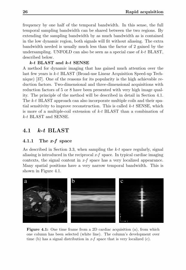
As described in Section 3.3, when sampling the k-t space regularly, signalaliasing is introduced in the reciprocal x-f space. In typical cardiac imagingcontexts, the signal content in x-f space has a very localized appearance.Many spatial positions have a very narrow temporal bandwidth. This isshown in Figure 4.1.

ba c

x

f

Figure 4.1: One time frame from a 2D cardiac acquisition (a), from whichone column has been selected (white line). The column’s development overtime (b) has a signal distribution in x-f space that is very localized (c).

4.1 k-t BLAST 27

Because one can control the sampling of k-t space, one can also controlhow the aliased signals are packed in the x-f space. It is not necessaryto sample the k-t space on an axis aligned grid. A sheared grid, forminga lattice, is still regular and will create periodic aliasing in the x-f space.The locations of the aliased signals will then also form a lattice. Using lat-tice sampling, the localized aliased signals can be packed tighter, enablingreduced sampling density in k-t space and thus faster acquisition. Twoexamples of k-t lattice sampling and the corresponding signal packing areshown in Figures 4.2.

k x

t fba

dc

k x

t f

Figure 4.2: Dense sampling on a k-t lattice (a) and the corresponding signalpacking in x-f space (b). Tight signal packing with no overlapping ensuresalias free reconstruction. Too sparse lattice sampling in k-t space (c), on theother hand, packs signals too tight in x-f space, causing overlapping and thusprohibits correct reconstruction.

Essentially, UNFOLD uses this principle, because the interlaced sam-pling pattern used in UNFOLD is also a lattice. A fixed predeterminedfilter is then used to recover the signal. The filter is a temporal low-passfilter with different bandwidths for the high and low dynamic regions. Theuse of a fixed filter imposes a limit on the packing, because the bandwidth


of the filter in the whole high-dynamic region must be wide enough to cap-ture the dynamics of the highest bandwidth in the region. The k-t BLASTapproach uses a filter more closely matched to the actual data, enablingpotentially tighter packing and thus higher reduction factors. Furthermore,this filter can be used to suppress signal where the aliased signals dominateover the main signal. This involves obtaining an estimate of the main signaldistribution without aliasing. This estimate can be used to further improveupon UNFOLD by using a reconstruction filter adapted to the measureddata.

4.1.2 Fast estimation of signal distribution in x-f space

Typical x-f signal distribution of cardiac objects have an additional prop-erty that can be exploited. The temporal bandwidth varies reasonablyslowly over the spatial dimensions. Especially, regions with low temporalbandwidth usually form large continuous regions. An estimate of the signaldistribution does not need to be of high spatial resolution [38], but onlyindicate where there is strong signal with high temporal bandwidth. Thesignal distribution estimate, sometimes referred to as training data, canthus be measured by sampling only the central lines in k -space. Becausean alias-free estimate is desired, these lines have to be sampled with fulltemporal bandwidth, i.e. sampled in every time frame.

A schematic illustration of the k-t BLAST approach is shown in Fig-ure 4.3. The k-t space is sampled using a sparse lattice, containing highresolution data with aliasing, and a dense region in the center of k -space inall time frames, containing information to estimate the signal distributionin x-f space. Since the sampling pattern is known, the positions of thealiased signals are also known. By knowing both an estimate of the trueand the aliased signal distributions, one can suppress aliasing in the signalreconstruction.

4.1 k-t BLAST 29

k

t

Reconstruction BLASTk−t

x

f

x

f

x

f

x

f

x

t

Low resolution signal estimateAcquisition matrix

data with aliasingHigh resolution

signalEstimated aliased

Filter output Reconstructed data

Figure 4.3: Schematic illustration of the k-t BLAST approach. Thek-t space is sampled in two ways. Central lines in k -space (triangles andblack circles) are fully sampled, yielding a low resolution estimate of the sig-nal distribution. The sparse lattice (triangles and hollow circles) yields highresolution data with aliasing. An estimate of the aliased signal can be obtainedfrom the signal estimate and sampling lattice. Through Wiener filtering, thealiasing can be suppressed, and a Fourier transform in time yields the finaloutput. The data used in this figure is the same as in Figure 4.1.


4.1.3 The k-t BLAST reconstruction filter

The measured signal from the lattice sample points is a sum of the truesignal and aliased signals, originating from other spatial locations and tem-poral frequencies. By treating the signal in each spatial position as wide-sense stationary in time, a Wiener filter approach can be used to filter outthe aliased signal. Furthermore, measurement noise is also expected, so theWiener filter becomes

M2

M2 +∑

M2alias + Ψ2

(4.1)

where M 2 is the signal distribution estimate,∑

M2alias is the estimated

aliased energy as shown in Figure 4.3 and Ψ2 is the measurement noisevariance.

The k-t BLAST reconstruction filter can be seen as a quotient betweenthe the desired signal energy estimate and the measured signal energy es-timate, consisting of the sum of the true signal, the aliased signal and themeasurement noise. Summing the signals in this way is appropriate for un-correlated signals. The aliased signal is from different spatial locations andtemporal frequencies, by lattice design, and correlation is thus expected tobe very low. The measurement noise is mainly caused by thermal noiseemitted by the subject and in the receiver electronics. The noise is Gaus-sian white [39], as long as one considers the complex signal measured. Themeasurement noise variance can be obtained by measuring the variancefor a homogeneous region in the image, such as the background. For re-construction of a wide-sense stationary source with wide-sense stationarynoise, the Wiener filter is the optimal linear estimator in the least squaressense [40].

The effect of the filter varies depending on the amount of signal overlapin x-f space. In areas with no overlap, the filter reduces to an ordinarynoise suppressing Wiener filter, passing signal where it is dominant overthe measurement noise. Where there is no true signal, the aliasing andnoise is efficiently removed. Where there is overlap, the filter will favor thedominant signal, passing signal if true signal is dominant or blocking signalif aliasing or noise is dominant.

This filtering process is intuitively performed by multiplication in thex-f space, but a corresponding convolution filter kernel in k-t space canalso be considered. Such a filter would fill in the blank positions in thek-t space which are not on the sampling lattice.

4.1 k-t BLAST 31

4.1.4 Implementation details

Lattice optimization

The locations of the aliased signals are determined by the sampling latticein k-t space. Thus, different sampling lattices can cause differing amountsof signal overlap and different reconstruction performance. Maximizing theminimum distance between the signal aliases can be done independently ofthe object being imaged, and is only dependent on field of view, temporalresolution and reduction factor [41]. Maximizing minimum alias distance,however, does not guarantee minimum overlap. To minimize overlap, theactual signal distribution for the particular acquisition has to be taken intoaccount, which is a much larger problem.

Reconstruction from arbitrary sampling in k-t space has been derived,but direct analytic solution to the problem was deemed infeasible due tocomputational complexity [37]. Iterative solution to this problem has beenpresented [42], enabling the use of non-Cartesian k-t BLAST. This may bevaluable even when using Cartesian lattice sampling, because the samplepoints will deviate from the lattice due to cardiac or respiratory phaseestimation errors.

Baseline subtraction

The temporal variation of the signal can be modeled as a deviation from abaseline signal. This baseline can be estimated by computing the temporalaverage of each k -space line. This baseline estimate is subtracted fromboth the signal distribution estimate and the lattice sampled data beforefiltering. The baseline is then added after the filtering step.

It is argued that treating this baseline separately will avoid reconstruc-tion errors that can otherwise be introduced in the filtering [37]. The base-line signal does contain the by far strongest signal which could warrantspecial treatment since it can be estimated in this alternative way.

Filtering the signal distribution estimate

Since the signal distribution estimate is obtained by measuring very fewlines in the central parts of k -space, and reconstructed by zero-filling theouter parts, ringing artifacts may occur. Therefore, some window, typicallya Hamming window, is used to reduce this ringing, though the benefits arereported to be subtle [38].

The original k-t BLAST paper [37] proposes temporal low-pass filter-ing of the signal distribution estimate, to reduce noise with high temporal


frequencies. This will also have the effect of suppressing high frequencysignals, effectively lowering achieved temporal resolution. Filtering the sig-nal distribution estimate itself will also have the unwanted side-effect ofunderestimating the high temporal frequencies of the aliased signal. Thiscan be avoided by performing the temporal low-pass filtering after applyingthe reconstruction filter.

Using signal distribution estimate twice

All points in k-t space not on the lattice are reconstructed from the lat-tice samples using the reconstruction filter in Eq 4.1. This includes thecentral k -space lines already acquired for the signal distribution estimate.Instead of using these reconstructed points, they can be substituted forthe measured data, especially if the central k -space lines were acquired inan interleaved fashion during the acquisition of the lattice samples. Themeasured central k -space lines can also be used in the baseline estimation.This will remove any aliasing in the lower spatial frequencies of the baselineestimate.

Chapter 5

Tensor field visualization

Visualization of tensor fields, a three dimensional volume where each pointis a tensor, is a difficult problem. The general concept of a tensor, a mul-tilinear mapping, is often impractical to visualize. Thus, many approachesare specialized for a particular application. In the case of myocardial de-formation, after eigen decomposition, three eigenvectors and correspondingeigenvalues are obtained. The eigenvectors of the strain rate tensors repre-sent the principal directions of instantaneous rate of shortening or length-ening. The eigenvalues indicate the rate of lengthening (positive value) orshortening (negative value). The tensor still has six degrees of freedom,making it impossible to solely use color coding.

5.1 Glyph visualization

A common way to visualize a tensor is to use a glyph, a geometric object,that can describe the degrees of freedom of the tensor. Such a glyph canfor instance consist of three arrows, representing the eigenvectors, scaledby their corresponding eigenvalues. Since the eigenvalues can be negative,this can be shown by the color of the arrow, or by making two arrows,pointing outward for positive eigenvalues or inward for negative eigenvalues,as in Figure 5.1a. A more intuitive way, especially in the application ofdeformation, is to visualize the tensor as an ellipsoid with the principal axesalong the eigenvectors and the corresponding radii set to some basis raisedto the power of the eigenvalue [43]. This would map negative eigenvalues toa radius between 0 and 1 and positive eigenvalues to a value larger than 1.The resulting ellipsoid would be the result of deforming a unit sphere withthis strain rate for some period of time. A two-dimensional example isshown in Figure 5.1b.

34 Tensor field visualization

a bFigure 5.1: Glyph visualization of deformation. Arrow glyph representationshowing eigenvectors and arrowheads indicate the sign of the eigenvalues (a).In the deformed circle visualization (b), the dashed unit circle represents anoriginal state and the ellipse represents the shape of the circle after beingdeformed according to the deformation indicated with the arrows. For visu-alization of strain rate, the ellipse represents a circle after being affected bythe strain rate for some period of time.

Using glyph rendering will allow description of all the degrees of freedomfor a tensor. The approach is thus good for a single tensor, but becomesimpractical for visualizing a whole field of tensors. Occlusion and visualcluttering makes this approach undesirable. The method suggested in Pa-per I is to separate visualization of a specific tensor of interest and the restof the tensor field. The idea is to show all degrees of freedom for one tensorusing glyph visualization, while some simplified global approach is used forthe underlying tensor field. The tensor of interest can then be changed bynavigating through the overview visualization.

5.2 Noise field filtering

A popular method in vector field visualization is Line Integral Convolu-tion (LIC) [44]. It works by convolving a noise field along line integralsof the vector field. The convolution kernel is a smoothing kernel, typi-cally a boxcar or Gaussian. The result, as illustrated in Figure 5.2, is apainting-like image with strokes along the vector field. The vector fieldis thus visualized using a scalar field, which basically contains structuredwhite noise. The resolution of the scalar field typically needs to be higherthan the resolution of the vector field, because structure with spatial extentis used to represent the vector value at a single point.

One of the advantages of LIC is that it preserves continuity of thevector field. The structures are connected along the vector field. LIC

5.2 Noise field filtering 35

baFigure 5.2: Two-dimensional LIC visualization for vector field visualization(a) of the vector field in (b). Note the continuous representation and lack ofdirectionality in the LIC visualization.

has been adopted for tensor visualization by performing the convolutionsequentially for the two dominant eigenvectors [45]. This is done withfixed convolution sizes, disregarding the degree of anisotropy, the relationbetween the eigenvalues, of the tensor field. The approach taken in Paper Iis instead to keep the main idea of LIC, starting with a noise field and filterit according to the tensor field. The output is a scalar field, with structurerepresenting the tensor field, that in the three dimensional case can bevisualized using volume rendering. The difference with respect to LIC isthat filtering is no longer performed along a line, but in a linear, planar orspherical fashion or somewhere in between, depending on the tensor field.Some kind of adaptive filtering is thus necessary.

5.2.1 Enhancement

A method that uses adaptive filtering controlled by a tensor field is imageenhancement [46, 47]. It is used to perform anisotropic low-pass filtering ofimages, avoiding filtering across edges and thereby blurring the image. Inthe first step, the local structure of the image is estimated into a structuretensor with the use of quadrature filters. This structure tensor containslarge eigenvalues in directions of strong edges. In two dimensions, a tensorwith two large eigenvalues corresponds to a point-like structure in the im-age, a tensor with one large eigenvalue corresponds to an edge and a tensor


with two small eigenvalues corresponds to a homogeneous region with nostructure. In the first case, no low-pass filtering will be performed. Inthe second case, anisotropic low-pass filtering will be performed along theedge (across the eigenvector direction). In the last case, isotropic low-passfiltering is performed. The method readily extends to higher dimensions.

The filtering is performed by steerable filters. Instead of constructinga new filter for each neighborhood, a set of filters is used, consisting ofone isotropic low-pass filter and several directed high-pass filters, as shownin Figure 5.3. The image is filtered using all filters, and the resultingoutput is produced by weighting the filter responses individually at eachpoint according to the structure tensor. If the low-pass filter is combinedwith a high-pass filter in some direction, the result is an all-pass filter inthat direction and a low-pass filter in the other directions. The high-passcomponents are added in directions with large eigenvalues, to preserve edgesalong these directions.

b c da

Figure 5.3: The filter set for two-dimensional steerable anisotropic filtering,consisting of one isotropic low-pass filter (a) and three directional high-passfilters (b-d). The filters can be combined linearly into an anisotropic low-passfilter of any direction.

The details of how the filter set is constructed and how the filter re-sponses are combined are described in Paper I.

In the image enhancement method, a structure tensor is estimated fromthe image, and the structure tensor is then used to control the filtering bysteering the filtering process. In the tensor visualization approach, the ten-sor field is already given. The image being filtered is an initial noise image.It is beneficial to iterate the filtering process in this case, in order to beable to create curved noise structures. In image enhancement, all-pass fil-tering is performed in directions of high eigenvalues and low-pass filteringis performed in directions of low eigenvalues. In visualization of strain ratetensors, the opposite is desired. This means low-pass filtering along strongeigenvalue directions, smearing the noise in these directions. The eigenval-ues are therefore remapped to facilitate this. A further improvement of themethod described in Paper I is to make use of the sign of the eigenvalue in

5.2 Noise field filtering 37

this mapping, similar to the mapping of eigenvalues to radii of the ellipsoid.The result is strong low-pass filtering along positive eigenvalue directions,medium low-pass filtering along zero eigenvalue directions and all-pass fil-tering along negative eigenvalue directions. In Figure 5.4, this is shownfor a systolic and a diastolic cardiac phase using volume rendering. One-directional volume preserving expansion, implying contraction in the othertwo directions, is thus visualized as spike-like structure in the expansiondirection. Correspondingly, volume preserving one-directional contractionis shown as disc-like structure. The resulting structure is thus reminiscentof the ellipsoid.

ba

Figure 5.4: Tensor visualization of strain rate tensors in the heart wall ofthe left ventricle in a short-axis slab in systole (a) and diastole (b). The right-ventricle has been excluded for the purpose of clarity. In three dimensions,there is spike appearance in systole, depicting radial expansion, and onionlayer appearance in diastole, depicting radial contraction.

This method can also been used to visualize other tensor fields. Oneexample is diffusion tensor data representing fiber structure in the brainmeasured with MRI. In this case, there are no negative eigenvalues, easingeigenvalue remapping. Fiber tractography, a popular method for visual-izing this type of data, creates a vector field out of the tensor data byexplicit tracking [48], but runs into problems at locations of fiber crossings


where the vector model is inappropriate. An intrinsic tensor visualizationapproach handles this automatically. The method described in Paper Ihas successfully been applied on diffusion tensor data [49], and an outputvolume is shown in Figure 5.5.

Figure 5.5: Volume visualization of fiber structure of the Corona Radiatain the human brain from two viewpoints. The volume is color coded accord-ing to the direction of the eigenvector corresponding to the largest eigenvalue(red = right–left, green = anterior–posterior, blue = superior–inferior). Cor-pus Callosum can be seen as the red structure. The green structures on top ofCorpus Callosum (top figure) are the Superior Longitudinal Fasciculus. Themotor-sensory fibers can be seen as the blue structure.

Chapter 6

Summary of papers

6.1 Paper I: Tensor Field Visualisation using

Adaptive Filtering of Noise Fields combined

with Glyph Rendering

This paper was presented at the IEEE Visualization conference in Boston2002. The paper presents a method for tensor field visualization that inte-grates visualization of a tensor-of-interest with an overview visualization ofthe complete tensor field. The idea is to use glyph rendering to show thetensor-of-interest with all degrees of freedom, while avoiding cluttering andocclusion associated with glyph rendering of tensor fields. The rest of thetensor field is then visualized using an alternative approach. A cursor canbe navigated through the background to change the location of the tensor-of-interest in real time. For the background visualization, a new methodinspired by line integral convolution is presented. A scalar field is createdfrom the tensor field with the use of tensor-controlled adaptive filtering. Anoise volume is used as a seed input and then iteratively filtered, creatingstructure in the noise in the directions of strong eigenvalues of the tensorfield.

6.2 Paper II: Five-dimensional MRI Incorporat-

ing Simultaneous Resolution of Cardiac and

Respiratory Phases for Volumetric Imaging

This paper presents a novel method for volumetric MRI acquisition tempo-rally resolved over both cardiac and respiratory cycles simultaneously. Thiscreates a five-dimensional data set, opening new possibilities for studying

40 Summary of papers

physiological effects caused by respiration on cardiac function. The methodis based on an alternative gating approach extended to two temporal dimen-sions. The acquisition is controlled in real-time by continuously estimatingcardiac and respiratory phase and sampling k -space individually for eachtime frame. The order of k -space traversal is optimized by using a Hilbertcurve which minimizes jumps in k -space. This reduces eddy currents thatcause artifacts when rapid pulse sequences are used.

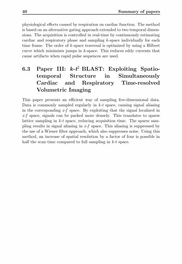
6.3 Paper III: k-t2 BLAST: Exploiting Spatio-

temporal Structure in Simultaneously

Cardiac and Respiratory Time-resolved

Volumetric Imaging

This paper presents an efficient way of sampling five-dimensional data.Data is commonly sampled regularly in k-t space, causing signal aliasingin the corresponding x-f space. By exploiting that the signal localized inx-f space, signals can be packed more densely. This translates to sparselattice sampling in k-t space, reducing acquisition time. The sparse sam-pling results in signal aliasing in x-f space. This aliasing is suppressed bythe use of a Wiener filter approach, which also suppresses noise. Using thismethod, an increase of spatial resolution by a factor of four is possible inhalf the scan time compared to full sampling in k-t space.

Chapter 7

Discussion

This thesis has presented new methods for imaging cardiac motion. Anal-ysis and visualization of local deformation was accomplished by computinga strain rate tensor field from a velocity field measured by MRI and visual-izing this tensor field using a combination of glyph rendering and overviewvisualization. The overview visualization was performed by volume ren-dering of a scalar field, computed by adaptive filtering of a noise field tocreate spatial structure. A method for volumetric imaging resolved overboth the cardiac and respiratory cycles simultaneously was presented, en-abling the study of interventricular coupling and septum shape in threedimensions, throughout the respiratory cycle. Acquisition efficiency wasincreased eight-fold by bandwidth sharing in x-f space, i.e. by packing thealiased signals tighter in x-f space.

7.1 Multidimensional imaging

This thesis presents imaging methods for high dimensional data. Myocar-dial deformation was represented as a tensor field with six degrees of free-dom in every point in a time-resolved volume. This corresponds to an innerdimension of six and an outer dimension of four. Imaging of anatomicalstructures in the five-dimensional approach, resolving the cardiac and res-piratory cycles in a volumetric acquisition, has an outer dimension of five.In Papers II and III, only scalar image data were acquired, i.e. having aninner dimensionality of one.

Routine clinical work as of today, on the other hand, often use tra-ditional methods in lower dimensions. Echocardiography measures ultra-sound reflectance or a one-directional Doppler shift in each sample point,corresponding to an inner dimension of one. This is performed along

42 Discussion

one spatial line over time in M-mode echocardiography. Two-dimensionalechocardiography extends this with one additional outer spatial dimension.There is no question that imaging in higher dimensions is more difficult andtime-consuming, and thus more expensive. One may ask oneself what theextra dimensions add to what is used in clinical practice today. When itcomes to physiological understanding, especially of the more complex inter-actions such as interventricular coupling or local myocardial deformation,directions and variations of motion is not known beforehand. Measuringmotion in only one direction imposes assumptions of the data, which in thehand of a skillful operator might be quite reasonable for some applications.For research purposes, however, objectivity is important, and the goal is toreduce sensitivity to operator dependent acquisition, slice positioning, slicemisregistration and angular error in velocity measurements. MRI studieshave stressed the need of a three-dimensional characterization of the shapeand curvature of the septum [50]. More comprehensive physiological un-derstanding can lead to better assumptions regarding motion directionalityand slice orientation sensitivity. This can then be transfered into lowerdimensional methods, and to clinical routine.

7.2 Using k-t2 BLAST for respiratory gating

k− t2 BLAST may be used as an alternative to respiratory gating. Insteadof acquiring data only in the end expiration period of the respiratory cycle,data can be acquired continuously, resolving the respiratory cycle. Thiswill commonly require longer scan times, due to the fact that the end ex-piration period usually accounts for about half the respiratory cycle, whileresolving the respiratory cycle to any desirable extent will require morethan two respiratory time frames. This increase in scan time can avoided ifk − t2 BLAST is used for scan time reduction. One may then after recon-struction select just one respiratory time frame to simulate a respiratorygated acquisition. An advantage is that this removes the necessity of priorknowledge of the optimal respiratory phase.

7.3 Costs of sparse sampling

The reduction of acquisition time in k-t BLAST comes from sampling thek-t space less densely. There are definitively drawbacks of the sparse sam-pling of data, such as increased noise and reduced temporal fidelity.

7.3 Costs of sparse sampling 43

7.3.1 Noise

It is in the nature of MRI that a shorter acquisition time means more noise.One may visualize this as foldover of noise, that the signal in x-f spaceis not really limited to the localized signal bearing parts, but there is awideband noise component as well. If there are fewer sampling pointsin k-t space, more noise will fold over the desired signal. The massivereduction factors typically used in k-t BLAST means that very few datapoints are acquired. This will have effects on noise. In the applicationof cardiac imaging, this extra noise is usually accepted in order to reduceimaging times or increase resolution. Since voxel sizes in typical cardiacexaminations are quite large, there is quite a lot of signal to begin with.Also, k-t BLAST carries an implicit Wiener filtering reducing the noisetemporally. Nevertheless, spatial filtering and especially spatiotemporalfiltering, along the lines of image enhancement [46, 47], might prove usefulto reduce noise when high spatial resolutions are approached. In the case offive-dimensional imaging, edges have a lot of structure that can be exploitedin noise reduction.

7.3.2 Temporal fidelity

The aim of the k-t BLAST method is to reduce imaging times withoutsacrificing image quality. When the signals in x-f space overlap, which isdifficult to avoid, some reconstruction error is unavoidable. The use ofthe Wiener filter minimizes this reconstruction error in the least squaressense, but there is still a reconstruction error. Overlapping mostly occursbetween high temporal frequencies of one spatial position and low temporalfrequencies of a different spatial position. The reconstruction error is mostprominent in high temporal frequencies. This is because the signal energy inthe lower temporal frequencies is much stronger than in the high temporalfrequencies and the optimal linear reconstruction from such overlap is toattenuate the least dominant signal. The result of this is a lower effectivetemporal bandwidth, i.e. temporal blurring.

This mechanism of alias overlap attenuation, suppressing the high tem-poral frequencies to retain the lower frequency content, will provide staticimages from k-t BLAST of very high quality. The aliasing which wouldarise if zero-filling reconstruction was performed will be minimized. Theloss of temporal bandwidth is only fully exposed in the temporal dimension,and since this dimension is omitted in static images, a false impression ofretained fidelity is presented. It is therefore important to study the tempo-ral dimension when using k-t BLAST. This can either be done with the use

44 Discussion

of animation or by using M-mode type visualization, where the temporaldimension is presented spatially.

The loss of temporal bandwidth is not equal to sampling with a lowerfrequency. Sometimes, high temporal bandwidth is used to suppress motionartifacts, not to resolve a particular temporal event. The temporal blurringcaused by k-t BLAST is done by filtering out the high frequency content,not letting it alias onto the lower frequencies. In this case, the loss ofeffective temporal bandwidth is not a loss of relevant image information.

With the use of short-TR pulse sequences, such as balanced SSFP, it ispossible to trade scan time for improved temporal resolution. By furtherapplying k-t BLAST, the original scan time can be restored. In this way,the original temporal bandwidth should at least be preserved, but hopefullyincreased, because the bandwidth will be shared between different spatialpositions. With a reduction factor of N, N different spatial positions willshare an N-fold bandwidth. If some spatial positions have low bandwidth,which is very common in cardiac imaging, more sampling bandwidth isavailable to the other positions. What remains to be studied is the practicalgain achievable and the cost of acquiring the signal distribution estimateand its effect on the accuracy of the Wiener reconstruction filter.

With two temporal dimensions, several parts of the k-t BLAST ap-proach can be controlled to act differently in each dimension. One may,for instance, adjust lattice optimization in order to preserve temporal fi-delity in one temporal dimension at the cost of increasing temporal blur-ring in the other dimension. Some applications desire high cardiac phasefidelity, but might accept a larger imaging window in the respiratory cycle,if k-t2 BLAST is used as a respiratory artifact reduction method. Otherapplications desire high respiratory phase fidelity, but can accept temporalblurring in cardiac phase dimension if the imaging is concentrated on theslow-varying diastolic cardiac phases.

7.4 Future work

7.4.1 Validation

The methods presented here need to be tested on more subjects and val-idated against other methods. One difficulty with validating the five-dimensional approach is that no other method produces similar data. Ro-bustness and reproducibility can be tested more easily, though, since it onlyinvolves testing a method against itself.

7.5 Potential impact 45

7.4.2 Tensor field data quality

The estimation of the strain rate tensor involves computing differentials,which in practice often is implemented by finite differencing. This meansthat the process is highly sensitive to noise and image artifacts. The impactof noise and artifacts on the scalar representation of the tensor field usedfor background visualization has not been studied. Nevertheless, the visu-alization results are likely to benefit from improvements in data acquisition,especially regarding noise and respiratory motion artifacts.

7.4.3 Optimizing reduction factor versus temporal fidelity

When using k-t2 BLAST, the effect of temporal blurring needs to be stud-ied. A large reduction factor is favorable for reducing scan time or increas-ing spatiotemporal resolution, but also increases risk of loosing importanttemporal information. The appropriate reduction factor needs to be op-timized for the individual applications. This is tightly coupled with thevalidation of the method.

7.4.4 Acquisition of velocity data using k-t2 BLAST

Two-dimensional phase contrast MRI measurements resolving both cardiacand respiratory cycles has been presented previously [18] and shows promiseof measuring important respiratory variations in blood flow. To this date,volumetric velocity acquisition resolved over both cardiac and respiratorycycles has not been performed. Five-dimensional acquisition in the formpresented in Paper II is too time consuming to add velocity measurements.Acquisition time shortening, along the lines of k-t2 BLAST presented inPaper III, is a prerequisite for five-dimensional velocity measurements. Notonly will these measurements be free of respiratory motion artifacts, asdescribed in Section 7.2, but it will also enable the studies of different flowpatterns in different phases of the respiratory cycle. The right ventricle hashighly respiratory dependent flow, and it’s complex shape is best describedusing a volumetric acquisition.

7.5 Potential impact

The tensor field visualization presented in Paper I may help investigatorsin the study of local myocardial deformation using fully three-dimensionalmeasurements. This may in turn be used to obtain new information as to

46 Discussion

which directions and locations of deformations are important for diagnosisor follow-up of certain diseases and treatments.

Volumetric imaging resolving both cardiac and respiratory cycles simul-taneously offers a completely new type of data. Study or quantification ofshape and ventricular volumes over the course of the respiratory cycle mayoffer new means for physiological description of interventricular coupling.The method presented in Paper II for measuring such a data set has thepotential to describe these phenomena.

Possibility to shorten acquisition time or increase resolution in cardiacimaging is always desired. The method presented in Paper III offers a wayto not only use temporal correlation in the cardiac cycle, but also in thecombined two-dimensional space of cardiac and respiratory cycles. This hasthe potential of reducing reconstruction error or allowing larger reductionfactors. This is not only applicable in reducing imaging time and increasingspatial resolution for volumetric imaging, but may also be applied to singleslice imaging for a far broader range of applications.

The k-t BLAST methods yield significant increase in imaging efficiency.There is no question that there is additional spatiotemporal structure inher-ent to the dynamics of cardiac and respiratory motion. Finding new waysto exploit these properties can open new possibilities and applications forcardiac MRI.

Bibliography

[1] Causes of Death 2003. Swedish National Board of Healthand Welfare (Socialstyrelsen), Epidemiologiskt Centrum, 2005.http://www.socialstyrelsen.se/.

[2] Hatle L, Sutherland GR. Regional myocardial function — a new ap-proach. Eur Heart J 2000;21(16):1337–1357.

[3] Guth BD, Schulz R, Heusch G. Time course and mechanisms of con-tractile dysfunction during acute myocardial ischemia. Circulation1993;87:35–42.

[4] Weber KT, Janicki JS, Shroff S, Fishman AP. Contractile mechanicsand interaction of the right and left ventricles. Am J Cardiol 1981;47(3):686–695.

[5] Santamore WP, Dell’Italia LJ. Ventricular interdependence: Signifi-cant left ventricular contribution to right ventricular systolic function.Prog Cardiovasc Dis 1998;40(4):289–308.

[6] Wranne B, Pinto FJ, Siegel LC, Miller DC, Schnittger I. Abnor-mal postoperative interventricular motion: new intraoperative trans-esophageal echocardiographic evidence supports a novel hypothesis.Am Heart J 1993;126(1):161–167.

[7] Waggoner AD, Shah AA, Schuessler JS, Crawford ES, Nelson JG,Miller RR, Quinones MA. Effect of cardiac surgery on ventricularseptal motion: assessment by intraoperative echocardiography andcross-sectional two-dimensional echocardiography. Am Heart J 1982;104(6):1271–1278.

[8] Lehmann KG, Lee FA, McKenzie WB, Barash PG, Prokop EK, DurkinMA, Ezekowitz MD. Onset of altered interventricular septal motionduring cardiac surgery. assessment by continuous intraoperative trans-esophageal echocardiography. Circulation 1990;82(4):1325–1334.

48 Bibliography

[9] Spencer AJM. Continuum Mechanics. Dover Publications, Inc., 1980.

[10] Axel L, Dougherty L. MR imaging of motion with spatial modulationof magnetization. Radiology 1989;171:841–845.

[11] Kvitting JPE, Sigfridsson A, Wigstrom L, Bolger AF, Karlsson M.Virtual makers for noninvasive assessment of myocardial dynamics. In54th Annual Meeting of the Scandinavian Association for ThoracicSurgery. Bergen, Norway, 2005; 150.

[12] Pelc NJ, Herfkens RJ, Shimakawa A, Enzmann DR. Phase contrastcine magnetic resonance imaging. Magn Reson Q 1991;7(4):229–254.

[13] Kvitting JPE, Ebbers T, Engvall J, Sutherland GR, Wranne B,Wigstrom L. Three-directional myocardial motion assessed using 3Dphase contrast MRI. J Cardiovasc Magn Reson 2004;6(3):627–636.

[14] Bracewell R. The Fourier Transform and its Applications. McGraw-Hill, 2nd edition, 1986.

[15] Lanzer P, Barta C, Botvinick EH, Wiesendanger HU, Modin G, Hig-gins CB. ECG-synchronized cardiac MR imaging: method and evalu-ation. Radiology 1985;155(3):681–686.

[16] Glover GH, Pelc NJ. A rapid-gated cine MRI technique. Magn ResonAnnual 1988;299–333.

[17] Fredrickson JO, Pelc NJ. Time-resolved MR imaging by automaticdata segmentation. J Magn Reson Imaging 1994;4(2):189–196.

[18] Fredrickson JO, Wegmuller H, Herfkens RJ, Pelc NJ. Simultaneoustemporal resolution of cardiac and respiratory motion in MR imaging.Radiology 1995;195(1):169–175.

[19] Scheffler K, Lehnhardt S. Principles and applications of balanced SSFPtechniques. Eur Radiol 2003;13:2409–2418.

[20] Jung BA, Henning J, Scheffler K. Single-breathhold 3D-TrueFISP cinecardiac imaging. Magn Reson Med 2002;48:921–925.

[21] Markl M, Leupold J, Hennig J. Double average parallel imaging foroptimized eddy current compensation and steady state storage in bal-anced SSFP imaging. In Proceedings of ISMRM. Miami Beach, 2005;503.

Bibliography 49

[22] Gotsman C, Lindenbaum M. On the metric properties of discretespace-filling curves. IEEE Transactions on Image Processing 1996;5(5):794–797.

[23] McKinnon GC. Ultrafast interleaved gradient-echo-planar imaging ona standard scanner. Magn Reson Med 1993;30:609–616.

[24] Noll DC, Nishimura DG, Macovski A. Homodyne detection in mag-netic resonance imaging. IEEE Trans Med Imag 1991;10(2):154–163.

[25] Nayak KS, Pauly JM, Yang PC, Hu BS, Meyer CH, , Nishimura DG.Real-time interactive coronary MRA. Magn Reson Med 2001;46:430–435.

[26] O’Sullivan JD. A fast sinc function gridding algorithm for Fourierinversion in computer tomography. IEEE Trans Med Imaging 1985;MI-4(4):200–207.

[27] Dutt A, Rokhlin V. Fast Fourier transforms for nonequispaced data.SIAM J Sci Comput 1993;14(6):1368–1393.

[28] Mistretta CA, Wieben O, Velikina J, Block W, Perry J, Wu Y, JohnsonK, Wu Y. Highly constrained backprojection for time-resolved MRI.Magn Reson Med 2006;55:30–40.

[29] Pruessman KP, Weiger M, Scheidegger MB, Boesiger P. SENSE: sen-sitivity encoding for fast MRI. Magn Reson Med 1999;42:952–962.

[30] Griswold MA, Jakob PM, Heidemann RM, Nittka M, Jellus V, WangJ, Kiefer B, Haase A. Generalized autocalibrating partially parallelacquisitions (GRAPPA). Magn Reson Med 2002;47:1202–1210.

[31] van Vaals JJ, Brummer ME, Dixon WT, Tuithof HH, Engels H, NelsonRC, Gerety BM, Chezmar JL, den Boer JA. ”Keyhole” method foraccelerating imaging of contrast agent uptake. J Magn Reson Imaging1993;3(4):671–675.

[32] Doyle M, Walsh EG, Blackwell GG, Pohost GM. Block regional inter-polation scheme for k-space (BRISK): a rapid cardiac imaging tech-nique. Magn Reson Med 1995;33:163–170.

[33] Korosec FR, Frayne R, Grist TM, Mistretta CA. Time-resolvedcontrast-enhanced 3D MR angiography. Magn Reson Med 1996;36:345–351.

50 Bibliography

[34] Hu X, Parrish T. Reduction of field of view for dynamic imaging.Magn Reson Med 1994;31:691–694.

[35] Madore B, Fredrickson JO, Alley MT, , Pelc NJ. A reduced field-of-view method to increase temporal resolution or reduce scan time incine MRI. Magn Reson Med 2000;43:549–558.

[36] Madore B, Glover GH, Pelc NJ. Unaliasing by fourier-encoding theoverlaps using the temporal dimension (UNFOLD), applied to cardiacimaging and fMRI. Magn Reson Med 1999;42:813–828.

[37] Tsao J, Boesiger P, Pruessman KP. k-t BLAST and k-t SENSE: Dy-namic MRI with high frame rate exploiting spatiotemporal correla-tions. Magn Reson Med 2003;50:1031–1042.

[38] Hansen MS, Kozerke S, Pruessmann KP, Boesiger P, Pedersen EM,Tsao J. On the influence of training data quality in k− t BLASTreconstruction. Magn Reson Med 2004;52:1175–1183.

[39] Sijbers J, den Dekker AJ, Audekerke JV, Verhoye M, Dyck DV. Es-timation of the noise in magnitude MR images. Magnetic ResonanceImaging 1998;16(1):87–90.

[40] Mallat S. A Wavelet Tour of Signal Processing. Academic Press, 1999.

[41] Tsao J, Kozerke S, Boesiger P, Pruessmann KP. Optimizing spatiotem-poral sampling for k−t BLAST and k−t SENSE: Application to high-resolution real-time cardiac steady-state free precession. Magn ResonMed 2005;53:1372–1382.

[42] Hansen MS, Baltes C, Tsao J, Kozerke S, Pruessmann KP, Eggers H.k−t BLAST reconstruction from non-cartesian k−t space sampling.Magn Reson Med 2006;55:85–91.

[43] Kirby RM, Marmanis H, Laidlaw DH. Visualizing Multivalued Datafrom 2D Incompressible Flows Using Concepts from Painting. InD Ebert, M Gross, B Hamann, eds., IEEE Visualization ’99. San Fran-cisco, 1999; 333–340.

[44] Cabral B, Leedom LC. Imaging Vector Fields Using Line Integral Con-volution. Computer Graphics 1993;27(Annual Conference Series):263–270.

Bibliography 51

[45] Hsu E. Generalized Line Integral Convolution Rendering of DiffusionTensor Fields. In Proceedings of the International Society for Mag-netic Resonance in Medicine, 9th Scientific Meeting and Exhibition,Glasgow, UK. 2001; 790.

[46] Knutsson H, Wilson R, Granlund GH. Anisotropic non-stationaryimage estimation and its applications — Part I: Restoration of noisyimages. IEEE Transactions on Communications 1983;31(3):388–397.

[47] Granlund GH, Knutsson H. Signal Processing for Computer Vision.Kluwer Academic Publishers, 1995. ISBN 0-7923-9530-1.

[48] Basser PJ, Pajevic S, Pierpaoli C, Duda J, , Aldroubi A. In vivo fibertractography using DT-MRI data. Magn Reson Med 2000;44:625–632.

[49] Sigfridsson A, Estepar R, Wigstrom L, Alberola C, Westin CF. Dif-fusion tensor visualization using random field correlation and volumerendering. In Proc. of th 9th International Workshop on ComputerAided Systems Theory. Las Palmas de Gran Canaria (Spain): Univer-sidad de Las Palmas de Gran Canaria, 2003; 41–45.

[50] Moses DA, Axel L. Quantification of the curvature and shape of theinterventricular septum. Magn Reson Med 2004;52:154–163.

multidimensional mri of cardiac motion

Documents