multicommodity facility location under group steiner
TRANSCRIPT

Multicommodity Facility Location under Group Steiner Access Cost
Laura J. Poplawski∗ Rajmohan Rajaraman†
AbstractMotivated by publish-subscribe mechanisms in networks, weintroduce a new class of multicommodity facility locationproblems: Multicommodity Group Steiner Facility Location(MGSFL). The input to MGSFL consists of a metric spaceover a given set of locations, a cost function which providesa building cost for each commodity at each location, a set ofclients located at various points in the metric, and the setof commodities that each client is interested in reaching. Asolution to MGSFL consists of (a) for each commodity, thelocations where facilities are built, and (b) for each client,a tree connecting the client to at least one facility for eachcommodity in its interest set. The goal is to minimize thesum of the total facility building costs and the metric costof the client trees.
MGSFL is a natural generalization of the well-studiedGroup Steiner Tree problem, which is equivalent to thespecial case of MGSFL in which every building cost is either0 or ∞ and there is only one client. We also note thatgiven the facility locations, the best client tree is an optimalsolution to an appropriate Group Steiner Tree instance.Since the Group Steiner Tree problem is hard to approximateto within a factor of Ω(log2−ε m) times optimum unlessNP has quasi-polynomial Las Vegas algorithms, where mis the number of commodities, the same hardness resultimmediately extends to MGSFL.
Our main result is a randomized 2O(√
log n log log n)-
approximation algorithm for MGSFL, where n is the num-
ber of clients. We also present deterministic poly-logarithmic
approximations for three special cases. We give an O(log n)-
approximation algorithm when the facility building costs
differ only by commodity, not by location. We present an
O(log4 n log m)-approximation algorithm when the interest
sets are laminar — i.e., for each pair of clients, either their
interest sets do not intersect or else one client’s interest set
is contained within the other client’s interest set. We end
with an O(log n)-approximation algorithm when there are
no building costs but each commodity must be built exactly
once.
1 Introduction
Facility location is one of the oldest and most well-studied algorithmic problems, applicable in widely di-verse areas such as business operations, network man-agement, and graph theory. Most existing multicom-modity facility location variants apply to cases in whichthe clients are physically moving between the facilitiesto obtain the various commodities. We are concerned
∗Raytheon BBN Technologies.†Northeastern University.
instead with a situation in which clients simply want toconnect to facilities serving various commodities. Thisis applicable, for instance, in the case of a publish-subscribe network in which clients are subscribers inthe network and commodities are content sources to bepublished. Each subscriber (a node in the network) iswilling to pay for only the least expensive set of edgesrequired to connect it to a source for each item of rele-vant published content. Content distribution networks(CDNs) give another real-world application: the CDNcontrols a set of links and wants to minimize both thecost of creating data caches and the link usage by itsend users. We can estimate the link usage by an enduser as the sum of the costs of the links necessary toconnect the user to its required caches.
These network-design applications lead to a fairlyconcrete problem definition which is a variation ofmulticommodity facility location. We are given a setof nodes (or clients) located in a network, plus a set ofcontent types (or commodities) that must be placed (afacility must be built) at nodes in the network. Eachclient is interested in some subset of the commodities,which we refer to as the interest set of the client.The interest graph is the bipartite graph of clientsand commodities with an edge from each client to thecommodities in its interest set. We are given the costfor each commodity to build a facility at each location(which may differ by commodity and by location). Wemust pay separately to build each commodity, even ifmultiple commodities are built at the same location.Each client will choose the minimum cost set of edgesthat connect it to some facility for each commodity inits interest set. In other words, each client will choosethe minimum Group Steiner Tree [18] that connects itto its interest set. Our goal is an algorithm to decidewhere to build each commodity to minimize the totalbuilding cost plus the total Group Steiner Tree costsfor the clients. We call this the Multicommodity GroupSteiner Facility Location problem (MGSFL).
From a theoretical perspective, MGSFL is partic-ularly interesting as a generalization of two distinctNP-complete problems: Facility Location (equivalentto MGSFL with one commodity) and Group SteinerTree (equivalent to MGSFL with a single client andwith each building cost set to either 0 or ∞). It is
already known that Group Steiner Tree cannot be ap-proximated to within a factor of Ω(log2−ε m) (where mis the number of commodities), even on trees, unless NPhas quasi-polynomial Las Vegas algorithms [11]. Anyapproximation algorithm for MGSFL will also give analgorithm for solving Group Steiner Tree.
1.1 Our Results Because we are working within anΩ(log2−ε m) bound on the hardness of approximatingMGSFL (where m is the number of commodities),we concentrate on a poly-logarithmic approximationratio. Our approach is to attempt a poly-logarithmicapproximation ratio on trees, and then apply the resultsfrom [7] to get an approximation algorithm for generalmetrics. In the following, we use n to represent thenumber of clients and m to represent the number ofcommodities.
• Building costs vary by commodity, not bylocation. (Section 3) We consider MGSFL ontrees when the cost of building each commodity isthe same regardless of where the facility is built.For this special case, which we show is APX-hard,we give a 9-approximation algorithm, implying anO(log n) approximation for general metrics.
• General MGSFL. (Section 4) Our main resultis a randomized 2O(
√log n log log n)-approximation al-
gorithm for general MGSFL. Our algorithm is anatural generalization of the Group Steiner Treealgorithm of Garg, Konjevod, and Ravi [8] using adependent rounding method, whose analysis maybe of independent interest.
Since we were unable to obtain a poly-logarithmic ap-proximation ratio for the general problem, we also ex-amine a version of MGSFL with specialized interestsets. Content and information sources are often orga-nized hierarchically; consequently, client interests canoften be represented together as a laminar graph. Weconsider the special case where the interest sets of theclients are laminar: given any two clients, either the in-terest sets do not intersect or else one client’s interestset is contained within the other client’s interest set.This version still has the same approximation hardnessbound, but it has nice properties that make the problemmore approachable.
• Laminar clients. (Section 5) We give anO(log3 n log m)-approximation algorithm for treemetrics when the interest graph is laminar by client,implying an O(log4 n log m) approximation for gen-eral metrics.
Often, k-median problems go hand-in-hand with fa-cility location problems, since this is the same problem
restricted to a certain number of buildings per commod-ity (instead of allowing unlimited buildings with a costper building). We consider only the 1-median version.
• 1-Median. (Section 6) We give an optimal de-terministic algorithm for the 1-median variant ofMGSFL on tree metrics with no building costs, im-plying an O(log n) approximation for general met-rics. This is the equivalent to the problem withbuilding costs varying only by commodity if allbuilding costs are very high compared to the edgelengths.
We conclude with some open problems in Section 7.
1.2 Related Work Variants of Facility Locationhave been studied for years. Single commodity versionsinclude uncapacitated ([19], [9], [14], [13], [15]), capaci-tated ([6], [16]), and k-median, in which at most k facil-ities can be built ([4], [1]). In [17], the first well-knownmulticommodity version, multiple commodities may bebuilt at the same facility with decreasing marginal cost.[17] gives an O(log t) approximation algorithm and amatching hardness result, where t is the maximum num-ber of commodities allowed at each facility. The resultsfrom [17] apply to the k-median version as well.
A Facility Location variant closely related toMGSFL — Group Facility Location — is discussed in[12]. In Group Facility Location, the goal is to opena set of facilities for each commodity, and each com-modity will build a Steiner forest (a set of trees rootedat the open facilities) connecting itself to all interestedclients. The goal is to minimize the sum over all com-modities of (1) the building costs plus (2) the cost of theSteiner forest for the commodity. This is different fromMGSFL because the commodities are building Steinerforests rather than the clients. Since a Group FacilityLocation algorithm chooses the locations for the com-modities, building forests around the commodities al-lows the algorithm to choose the roots of the forests. InMGSFL, however, the roots are fixed and an algorithmdetermines the leaves, yielding a different problem froma technical standpoint.
Since each of our clients is solving the GroupSteiner Tree problem, introduced in [18], our results alsobuild on previous work related to Group Steiner Tree.[8] gives a randomized O(log n log m)-approximationalgorithm for Group Steiner Tree on a tree, where n isthe number of nodes and m is the number of groups.[3] derandomizes the algorithm from [8]. [10] givesan Ω(log2 m) lower bound on the integrality ratio ofGroup Steiner Tree, even on trees, and this is extendedto an Ω(log2−ε m) approximation lower bound in [11].[5] provides a combinatorial algorithm with a poly-

logarithmic approximation ratio.MGSFL is also a generalization of the multicast
“push-pull” data dissemination problem introduced in[2]. In fact, one problem discussed in [2] is preciselya 1-Median version of MGSFL in which exactly twoclients are interested in each commodity. [2] alsoconsiders a number of other problem variations thatdiffer significantly from MGSFL.
2 Formal Definition
An instance of MGSFL is defined by a tuple〈V,E, M, I, d, c〉, in which V is the set of nodes, E is theset of edges, M is the set of commodities, I : V → Zis the interest set function, d : E → Z is the lengthfunction, and c : M × V → Z is the building cost func-tion. The interest set of v, I(v), represents the set ofcommodities in which node v is interested. The lengthof edge e = (u, v) is d(e) or d(u, v). The cost of buildinga facility for commodity t at node v is c(t, v). We willuse n = |V | and m = |M | for notational convenience.We refer to any node with a nonempty interest set as aclient. Our formulation allows at most one client at anynode. This is without loss of generality since multipleclients at a node can be modeled by simply creating anew node for each client connected by 0 length edges.
A solution to an MGSFL instance consists of acollection of location sets Lt : t ∈ M and a collectionof trees Sv : v ∈ V ; Lt specifies the nodes at which afacility for commodity t will be built, and Sv connectsv to at least one node in Lt for each t ∈ I(v). When thetree Sv successfully includes a node at which a facilityfor t ∈ I(v) has been built, we say that client v meetscommodity t. We extend the length function d anddefine d(Sv) to be the sum of lengths of the edges in Sv.An optimal solution to the MGSFL instance minimizesthe following. ∑
v∈V
d(Sv) +∑t∈M
∑v∈Lt
c(t, v)
In the special case where there is only one client andeach building cost is set to be either 0 or ∞, MGSFL isequivalent to the well studied Group Steiner Tree prob-lem [18, 8, 3, 10, 5], in which we are given m groups ofnodes and want to find the minimum cost tree connect-ing a given root node to at least one node from each ofthese groups. It is known that even when the underlyinggraph is a tree, Group Steiner Tree cannot be approx-imated to within Ω(log2−ε m) (where m is the numberof groups) unless NP has quasi polynomial Las-Vegasalgorithms [11]. Thus, our focus in this paper is onpoly-logarithmic approximations for MGSFL. We use astandard approach toward this goal: we concentrate onsolving MGSFL on trees, and invoke metric embedding
machinery [7] to derive results for general metrics. From[7], there is a randomized embedding from any metricinto a tree with maximum distortion O(log n) (wheren is the number of nodes in the metric), so any solu-tion on a tree with approximation ratio R will achieveapproximation ratio O(R log n) on an arbitrary metric.
Henceforth, we concentrate on algorithms forMGSFL when the underlying graph is a tree T =(V,E). We add the following additional notation. Leth(T ) be the height of a tree T , Puv be the unique pathconnecting nodes u and v in T , auv be the least commonancestor of nodes u and v in T , Te be the subtree of Trooted at and including edge e, and Tu be the subtree ofT rooted at node u. We also assume that all clients arelocated at the leaves, and that all commodities must bebuilt at leaves. This does not restrict our problem, sincewe can always add an edge of length 0 to each node inthe graph, effectively converting our non-leaf nodes intoleaves.
For the benefit of the reader, Table 1 summaries theabove notation.
T = (V,E) A tree consisting of nodes (V )and edges (E)
n The number of nodes (|V |).Te, Tu The subtree of T rooted at edge
e, node u.h(T ) The height of tree T .Puv The set of edges along the unique
path in T from node u to node v.auv The least common ancestor of
nodes u and v in T .d(e), d(u, v) The length of edge e = (u, v).M , m The set of all commodities (M)
and the number of commodities(m).
I(v) The subset of commodities inwhich the client at node v is in-terested.
c(t, v) The cost of building a facility forcommodity t at node v.
Sv The group Steiner tree used forclient v to connect it to all com-modities t ∈ I(v).
Table 1: Notation
Linear Program for MGSFL. Many of our algo-rithms use the following linear program, which givesa fractional solution to MGSFL on a tree, assumingwithout loss of generality that we may only build com-modities at the leaves.
In the LP, the variable ytu represents the amountcommodity t is built at node u, xjtu represents theamount client j meets commodity t at node i, and zje
represents the amount client j crosses edge e.minimize∑
j,e
zje · d(e) +∑u,t
ytu · c(u, t)
subject to
zje ≥∑
u:e∈Pju
xjtu for all j, t, e
(2.1)
∑u
xjtu ≥1 for all j, t ∈ I(j)(2.2)
ytu ≥xjtu for all j, t, u(2.3)
ytu =0 for all t, for all u not at a leafytu ≥0 for all t, u
xjtu ≥0 for all j, t, u
zje ≥0 for all j, e
In addition, we want to set the following, which willbe used in the algorithms. Notice that wjte and wjtv areeach at most 1 for any j, t, e, v.
• wjtu =∑
v∈Tuxjtv
• wjte =∑
v∈Texjtv
• Ytu =∑
v∈Tuytv
Since the LP gives a fractional solution to MGSFL,we may describe the fractional solution with suchphrases as “client j meets commodity t at least 1
4 insubtree Te” or “commodity t is built at most 1
2 at nodev.” A fractional meeting of amount δ between j and t atv means that mine∈Pjv
zje ≥ δ and ytv ≥ δ. A fractionalbuilding amount δ for t at v means ytv ≥ δ.
It is worth noting that the same linear program,appropriately specialized, has been used to solve theGroup Steiner Tree problem [8, 3, 10, 5]. Therefore theintegrality ratio of this LP is at least Ω(log2 m) in thegeneral case, as proved in [10].
We close this section with the following Theoremproved in [5], and an immediate Corollary, which weuse later in this paper. For a given tree T , let h(T )denote the height of T and let dT (u, v) represent thedistance between nodes u and v in T .
Theorem 2.1. Chekuri, Even, Kortsarz [5, Section 4]Then, we can find another tree T ′ such that h(T ′) ≤3 · logα n, and for any u, v, dT (u, v) ≤ dT ′(u, v) ≤α · dT (u, v).
Corollary 2.1. Given a tree T with n nodes, we canfind a tree T ′ with h(T ′) ≤ O(
√log2 n), and for any u,
v, dT (u, v) ≤ dT ′(u, v) ≤ O(2√
log2 n) · dT (u, v).
3 Building costs vary by commodity, not bylocation
In this section, we restrict the building cost functionso that c(t, v) = c(t, v′) for all t, v, v′ 6= v. For thisspecial case, we present a polynomial-time O(log n)-approximation algorithm. We achieve this by develop-ing a 9-approximation algorithm for tree metrics, andthen invoking the metric embedding machinery. Be-fore we present our algorithm for the tree, we show thatMGSFL problem is APX-hard, even for the special casewhen all building costs are uniform and the underlyingnetwork is a tree. This implies, our approximation fortrees is within a constant factor of the best achievableunless P 6= NP.
Theorem 3.1. When building costs are uniform,MGSFL is APX-hard even for tree networks.
Proof. The proof is by reduction from set cover. LetS be a set cover instance with U being the universeof n elements, and S being the collection of sets. Weassume furthermore that each set consists of at most Belements, and the number of sets an element belongsto is at most B. We construct an MGSFL instance〈V,E, M, I, d, c〉 as follows. The set V equals S ∪ rwhere r is a special root node. The set E of edgesequals (r, s) : s ∈ S. We have a commodity for eachelement, so M equals U . The length of every edge is 1and the cost of building any commodity at any locationis C (C > 1). At every leaf node s, for every commodityt ∈ s, we have k clients each with interest set equal tos, where k is chosen to be larger than 2Cn2. Finally,we have one client at the root with interest set equal toU .
We now consider solutions to the MGSFL instance.One solution X is to build a facility for commodity tat leaf s whenever t is in s, and for the client tree ofthe client at root r to be formed by connecting theroot to the leaf nodes in a subset S′ of S that formsthe minimum set cover solution to S. The cost of Xequals opt(S) + C
∑s∈S |s|, where opt(S) is the cost of
a minimum set cover. opt(S) < n, since the n nodesinclude |S| leaves plus one root, while opt(S) includesat most all |S| sets. C
∑s∈S |s| ≤ C|S|B < Cn2.
Consider any solution Y . If there exists a leaf nodes and a commodity t ∈ s such that no facility for t isbuilt at s, then the cost incurred by the k clients tomeet commodity t is at least k. Since k > 2Cn2 (whichexceeds the cost of X), Y is optimal only if at every leaf

s a facility is built for every commodity in s; otherwise,we can replace Y by another solution that has smallercost and satisfies this property. Furthermore, we canassume without loss of generality that no facility is builtat the root since any such facility can be removed, andat most one edge added to the root client tree whilesaving at least C − 1 > 0 cost. Thus, the set T ofleaves where the root client meets the commodities inU \R is a valid set cover solution. The cost of Y equalsC∑
s∈S |s| + cost(T ), where cost(T ) is the cost of theset cover solution T .
Suppose we obtain an α-approximation to theMGSFL instance. Then, we obtain a solution to theset cover instance of cost at most (α − 1)C
∑s∈S |s| +
αopt(S), which is at most (α − 1)CBn + αopt(S).Since opt(S) is at least n/B, we obtain that we havea solution to the set cover instance with cost at most((α− 1)CB2 + α)opt(S). Since C and B are constants,we can set α+(α−1)CB2 to be a constant strictly biggerthan 1 by setting α sufficiently close to 1. Given that theset cover problem, even with the restriction of boundedset sizes and bounded number of occurrences for eachelement, is APX-hard, it follows that the MGSFL prob-lem with the restriction that the underlying network isa tree and building costs are uniform, is APX-hard.
We next present our algorithm. We round a solutionto the LP using Algorithm 1. Algorithm 1 builds three“types” of facilities. Examining one commodity at atime, we skim down the tree in a depth-first searchorder, starting at the root. We built the first type ofcommodity, Type A, at some node u if there are twosubtrees rooted at children of u such that the LP builtthe commodity at least 1
3 in each of these subtrees. Aswe skim down the tree, each time we’ve accumulatedanother unused 1
3 of built facility for the commodity,we build a Type B facility. If we hit a point where nosubtree has at least 2
3 total building for the commodity,then we build a facility of Type C and stop building thiscommodity down this path.
Theorem 3.2. Algorithm 1 gives a 9-approximationto MGSFL on a tree, when for any t, v, v′, c(t, v) =c(t, v′).
Proof. Lemmas 3.1 and 3.2 together prove Theorem3.2.
Lemma 3.1. After an execution of Algorithm 1, eachclient j meets each commodity t ∈ I(j) at least once.
Proof. Consider client j interested in commodity t.Consider some subtree (say it is rooted at r0) such thatwjtr0 ≥ 1
3 in the LP solution, and such that for any child
Algorithm 1 Approximation algorithm for the versionof MGSFL with no budget and with building costsvarying only by commodity, not by location.1: Solve the LP.2: for each commodity t do3: for each node r0 in the tree, in a depth-first-
search order do4: Let (r0, r1, r2, . . . , rf ) = the nodes along the
path from r0 to the root of the tree (rf ).5: if Ytr0 ≥ 1
3 then6: if there are no“Type C” buildings for com-
modity t along path (r1, r2, . . . , rf ) then7: if there are two children c1 and c2 of r0
such that Ytc1 ≥ 13 and Ytc2 ≥ 1
3 then8: build a Type A facility for commodity t
at r0
9: else10: Let ri be the closest node to r0 in
the path (r0, r1, . . . , ri, . . . , rf ) such thatwe’ve built a Type B facility for com-modity t at ri. If we have not built anyType B facilities, let i = f + 1.
11: if∑i−1
x=0
∑children r of rx such that Ytr< 1
3Ytr ≥
13 then
12: build a Type B facility for commodityt at r0
13: else if there is no child c of r0 such thatYtc ≥ 2
3 then14: build a Type C facility for commodity
t at r0
15: For each client j, let Sj = the set of all edges e suchthat zje ≥ 1
3 .
r of r0, wjtr < 13 . Say (r0, r1, . . . , rf ) is the path from
r0 to the root of the tree. Then any node in (r0, . . . , rf )satisfies the condition on line 1 by definition of r0. Wewill show that j must meet t at some ri.
Claim 3.1. If we built a facility of Type C for com-modity t at any node ri in (r0, . . . , rf ), then our tree forclient j must include ri.
Proof. Suppose there is a Type C facility at node ri(0 <i ≤ f). Since the condition on line 1 was true (we builta Type C facility), Ytri−1 < 2
3 . Therefore, j meets t lessthan 2
3 in the subtree rooted at ri−1. If j is a descendantof ri−1, the LP solution for j must include edge (ri−1, ri)with weight at least 1
3 in order for j to meet t at leastonce in the tree. Therefore, our solution tree for client jmust include ri. If j is not a descendant of ri−1, the LPsolution for j must include edge (ri, ri−1) at least 1
3 inthe LP solution to get to r0 (by definition of r0), so our
solution tree for client j will still include ri. Therefore,j meets t at ri.
Claim 3.2. Suppose there is a facility for commodity tat node ri(0 < i ≤ f), and there are no facilities for tbuilt at any rg, 0 ≤ g < i. Then, our tree for client jmust include ri.
Proof. Since we didn’t build a facility at any rg, 0 ≤g < i, we could not have built a Type B facilityat any of these nodes. Therefore, since we didn’tbuild a Type B facility specifically at r0, then by line1,∑i−1
x=0
∑children r of rx:Ytr< 1
3Ytr < 1
3 . Furthermore,since we didn’t build a Type A facility at any rg, 0 <g < i, the condition on line 1 must also be false forthese nodes, so Ytc < 1
3 for all children c of rg, c 6= rg−1
(by definition of r0, we know that all nodes c on thepath r0, r1, . . . , rf have Ytc ≥ 1
3 ). We also didn’t builda Type A facility at r0, so at most one child c of r0 hasYtc ≥ 1
3 . We didn’t build a Type B facility at r0, sothere must be one child, say r−1 of r0 with Ytr−1 ≥ 1
3 .By definition of r0, j meets t < 1
3 under each child ofr0, including r−1. This gives:
∑children r 6=r−1 of r0
Ytr +∑i−1x=1
∑children r of rx,r 6=rx−1
Ytr < 13 , so j meets t less
than 13 under any children of this path other than r−1,
and j meets t less than 13 under r−1. So j meets t less
than 23 under ri−1.
If j is a descendant of ri−1, the tree for j in theLP solution must include edge (ri−1, ri) at least 1
3 , soour tree for j will include ri. If j is not a descendant ofri−1, it must pass through ri at least 1
3 to get to r0 (bydefinition of r0). So j meets t at ri.
If there is any facility for commodity t built at r0, jwill meet t there, since j passes through r0 by definitionof r0. Therefore, if there is a facility for commodity tbuilt at any node in (r0, . . . rf ), j will meet t.
If no facility is built at any node in (r0, . . . rf ), thent must be built ≥ 1
3 in at most one child of r0 (but meetsj there less than 1
3 ), and other than this subtree underr0, t is built a total of < 1
3 under rf . So j meets t < 23
under rf , a contradiction since rf is the root of the tree.Thus there must be some facility for t built at a
node in (r0, . . . rf ) which is part of our tree for j.
Lemma 3.2. The cost from Algorithm 1 is at most 9times the cost of the solution to the LP.
Proof. The client costs incurred by Algorithm 1 are atmost 3 times the LP client cost, since the client valueszje are either rounded down to 0 or multiplied by 3.
We will analyze the building costs for a singlecommodity, t, according to the type of facilities built.
Type A facilities: If X is the number of lowest levelsubtrees Tu in which the LP solution gives Ytu ≥ 1
3(“lowest level” means that although the LP builds tat least 1
3 in the subtree Tu, the LP builds t lessthan 1
3 under each subtree rooted at a child of u), wemay build at each intersection of two such subtrees.The maximum number of such intersections equalsthe maximum number of non-leaf nodes with at least2 children in a tree with X leaves. Therefore, themaximum number of such intersections is less than X.This gives us a cost less than 3 times the LP cost forbuilding facilities.
Type B facilities: These are paid for bythe“gathered” costs from the subtrees in which the com-modity is built < 1
3 by the LP. In other words, we areconsolidating the cost of tiny fractions of built facilitiesover a number of subtrees and using each of these tinyfractions only towards a single facility. Since each frac-tional building in the LP is used to build at most oneType B facility, and since we must have at least 1
3 of abuilding for each type B facility we build, this cost is atmost 3 times the LP cost for building facilities.
Type C facilities: These are paid for by the > 13
building below the node at which the Type C facility isbuilt. Again, we pay at most 3 times the LP cost forbuilding facilities.
We now bound the total cost. The fractionalbuilding cost at a node u in the LP may be used tobuild a Type C facility only at ancestors of u. No otherfacility will be built at any node whose ancestor containsa Type C facility (according to the condition at line 1of the algorithm). Therefore, if the same cost at u isalso used towards a Type B facility, the Type B facilitymust be located at an ancestor of the Type C facility.By the condition at line 1, facilities of any type are onlybuilt at the root of a subtree in which there is > 1
3 builtby the LP, so the LP must build the commodity > 1
3 inthe subtree rooted at the Type C facility. However, thecost of a Type B facility comes entirely from subtreeswith < 1
3 built by the LP. Therefore, the fractionalbuilding at u cannot be used towards both a Type Cand a Type B facility. This means that our buildingcosts are at most the LP building costs times [ the costfor building Type A facilities times the maximum of(Type B building costs, Type C building costs)] ≤ 9times the LP building costs.
We can use the probabilistic embedding techniquefrom [7] to convert the problem on general metrics to theproblem on trees, adding only a factor O(log n) to theapproximation ratio. Therefore, this algorithm gives anO(log n)-approximation on general metrics.

4 General MGSFL
In this section, we give a 2O(√
log n log log n) approxima-tion algorithm for the general MGSFL problem. Ouralgorithm uses a generalization of the elegant random-ized rounding algorithm of [8] for Group Steiner Treethat may be of independent interest.Height reduction. First, we will convert the inputtree into a tree with at most
√log n levels. This can be
done as in Corollary 2.1, giving up a factor of 2√
log n inthe approximation ratio.Solving LP and preprocessing. Next, we solvethe LP applied to the tree of reduced height. Beforerounding, we ensure that each of our variables has avalue ≥ 1
2n , and each xjtu variable has a value < 18 . To
make sure all values are at least 12n , we will (a) set any
value below 12n to 0, and (b) double all remaining values.
All LP constraints still hold after each of these stepsexcept for Constraint 2.2, which will break after step(a). However, we’ve only removed at most n · 1
2n = 12
from the left hand side, so by doubling the values instep (b), we get back to a valid (although non-optimal)solution. We have at most doubled the value of theobjective function, and we are now assured that eachvalue is at least 1
2n . To ensure that each xjtu < 18 , we
proceed as follows. For any j, t such that there existssome xjtu ≥ 1
8 , pick one such u. Set xjtv = 0 for all v,set ytu = 1, and set xje = 1 for all e ∈ Pju. Now wehave guaranteed that j and t will meet at node u, andwe have at most multiplied the objective function by anadditional 8.Rounding. The core of the algorithm is the followingrandomized rounding procedure. We set new variablesw′
jte, x′jtu, y′tu, and z′je (each will be 0 or 1). Initially,set w′
jte = 0. Follow the steps below.
1. For each edge e, assign a random value re ∈ [0, 1].
2. For each client j, commodity t ∈ I(j), and edgee . Assume the path from the root to e ise1, e2, . . . , ep = e. Set w′
jte = 1 if and only ifwjte1 ≥ re1 and wjteα
wjteα−1≥ reα
for all α ∈ 2, . . . p.
3. For each client j, commodity t ∈ I(j), leaf u: setx′jtu = 1 if and only if w′
jte = 1 for e adjacent toleaf u.
Finally, set y′tu = 1 if and only if ytu = 1 or there is somej such that x′jtu = 1. Set z′je = 1 if and only if zje = 1or e is on the path from j to some u with x′jtu = 1.
The above algorithm does not guarantee that eachclient meets all commodities in its interest set (or eventhat all commodities have been built). Therefore, wewill repeat the algorithm, including the union of theresults, until all requirements are met.
Our analysis proceeds as follows. We will startin Lemma 4.1 by analyzing the expected cost of oursolution. Then, in Lemma 4.2, we show that there isa high probability that a given client will meet a givencommodity in its interest set. Finally, we compute howmany times we can expect to repeat the algorithm toachieve an arbitrarily high probability that each clientmeets all commodities in its interest set. Our totalexpected cost is the expected cost of a single iterationtimes the number of iterations.
Lemma 4.1. From the above rounding steps 1 to 3, weget
E
∑j,e
z′je · d(e) +∑t,u
y′tu · c(u, t)
]≤
2O(√
log n log log n) ·∑j,e
zje · d(e) +∑t,u
ytu · c(u, t)
Proof. We start by analyzing this for a single y′tu.Suppose the path to u is made up of edges e1, . . . , ep.For ease of notation, let vj1 = wjte1 , and vjα = wjteα
wjteα−1
(for each client j interested in commodity t). With thismodified notation, y′tu = 1 if and only if there existssome j such that vjα ≥ reα for all α. Furthermore,∏p
α=1 vjα ≤ ytu, since wjtep is the only term that doesnot cancel (which is exactly xjtu), and by LP Constraint2.3, xjtu ≤ ytu. We will artificially increase the finalvalue (vjp) for each client so that each client has exactly∏p
α=1 vjα = ytu. This will only increase the expectedvalue of y′tu.
Now we are looking at a series of p-dimensionalpoints Vj = (vj1, . . . , vjp) that each satisfy∏p
α=1 vjα = ytu, plus one randomly chosen p-dimensional point R = (re1 , . . . rep). y′tu = 1 if andonly if there exists some j just that R ≤ Vj in each di-mension. We can upper bound this probability by theprobability that R will lie underneath the p-dimensionalcurve
∏pα=1 xα = ytu where each variable ranges from
ytu to 1. This is illustrated for a 2-hop path in Figure1.
The area above the curve is given by the following

Figure 1: Analyzing the probability that a commodity ywill be built at some leaf of a tree with depth 2. For thedata plotted in this graph, ytu = 1
8 . Each client meetst with probability ytu in the LP solution. Any possiblevalues of vj1 and vj2 for clients j meetings commodity tat this node are represented by points along this curve. twill be built here only if our random point R = (R1, R2)lies in the gray area under this curve.
integration.∫ 1
ytu
∫ 1
ytuxp
∫ 1
ytuxpxp−1
. . .
∫ 1
ytuxpxp−1...x3
∫ 1
ytuxpxp−1...x3x2
dx1dx2 . . . dxp−1dxp
= 1− ytu −p∑
i=1
(−1)i(ytu
i!
)lni
(1
ytu
)
= 1− ytu −p∑
i=1
(ytu
i!
)lni
(1
ytu
)Subtracting the above expression from 1 will give
the area under the curve, so our actual upper bound onthe expectation of building commodity t at node u is
ytu +p∑
i=1
(ytu
i!
)lni
(1
ytu
)
= ytu ·
1 +p∑
i=1
lni(
1ytu
)i!
≤ ytu ·
1 +p∑
i=1
lni(
1ytu
)i!
After solving the LP, we took steps to ensure that
all ytu values were at least 12n , so lni(1/ytu)/i! is at
most lni(2n)/i!, which by Stirling’s approximation is atmost ((e lnn)/i)i. Since 1 ≤ i ≤ p, and p is the heightof the tree which is at most O(
√log n), lni(1/ytu)/i!
is maximized at i = p yielding an upper bound of(e√
log n)√
log n. We thus have the following upperbound on the expected cost of building commodity tat node u.
E[y′tu] ≤ ytu ·
1 +p∑
i=1
lni(
1ytu
)i!
≤ (p + 1)
(e√
log n)√log n
· ytu
= 2O(√
log n log log n) · ytu
We next bound E[z′je] in terms of zje. First, assumee is an edge adjacent to a leaf u, and assume the partof the path from j to u is made up of edges e1, . . . , ep.As above, let vt1 = wjte1 and vtα = wjteα
wjteα−1(for each
commodity t in which client j is interested). Then,z′je = 1 if and only if there exists some t such thatvtα ≥ reα for all α.
∏pα=1 vtα ≤ zje (as above), since
wjtep is the only term that is not cancelled (which isexactly xjtu), and by LP Constraint 2.1, xjtu ≤ zje.We will artificially increase the final value (vtp) foreach commodity so that each commodity has exactly∏p
α=1 vtα = zje. Now we can solve the same integral asabove to get E[z′je] = 2O(
√log n·log log n) · zje.
Now we need to consider an edge e that is notadjacent to a leaf, and may therefore be on the pathto more than one leaf. Assume the edges on the pathfrom j to e are e1, . . . , ep = e. We set z′je = 1 if andonly if e is on the path to some u with x′jtu = 1. Inorder for any one of these x′jtu to be 1, it must bethe case that wjte1 ≥ re1 , and wjteα
wjteα−1≥ reα for all
α = 2 . . . p. For any commodity t, the product of thesevalues is exactly wjtep = wjte ≤ zje (by definition ofw). Now we can apply the same logic as before to showE[z′je] = 2O(
√log n·log log n) · zje
Adding these together and applying linearity ofexpectation, we complete the proof of the theorem.
E
∑j,e
z′je · d(e) +∑t,u
y′tu · c(u, t)
≤ 2O(
√log n log log n) ·
∑j,e
zje ·
(d(e) +
∑t,u
ytu · c(u, t)
)Next, we will use Janson’s inequality to bound the
probability that a given client-commodity pair does not

meet in the rounded solution. This probability is lowenough that we can bound the number of expectediterations before all requirements are met. We start bydefining Janson’s inequality. We borrow the followingnotation from [8]. Let Ω be a universal set, and R ⊆ Ωdetermined by the experiment in which each elementr ∈ Ω is independently included in R with probabilitypr. Let Ai be subsets of Ω, and denote by Bi theevent that Ai ⊆ R. Write i ∼ j if Bi and Bj are notindependent. Define ∆ =
∑i∼j Pr[Bi ∩Bj ] (the sum is
over ordered pairs). Let µ =∑
i Pr[Bi], and ε be suchthat Pr[Bi] ≤ ε for all i.
Theorem 4.1. (Janson’s inequality) With the no-tation as above, if ∆ ≥ µ(1 − ε), then Pr[∩iBi] is atmost e−µ2(1−ε)/(2∆).
The proof of the next lemma is adapted from [8].
Lemma 4.2. For a given client j and commodity t ∈I(j), assuming xjtu < 1
8 for all u, the above steps 1to 3 will set x′ values that satisfy LP Constraint 2.2(∑
u xjtu ≥ 1) with probability at least 1− e−7
16√
log n .
Proof. We will set the variables defined above for usewith Janson’s inequality. First find the first edge falong the path from j to the root with zjf = 0. Ωwill be the set of all edges (not on the path from j tof) in the subtree rooted at f . For each edge e ∈ Ω wewill define pe as follows. Assume e has parent edge e′
(e′ is the next edge along the path from e to f). If e isadjacent to aue, pe = wjte. Else, pe = wjte
wjte′.
Define a subset Au for each node u that has xjtu >0: Au is the set of all edges along the path from aju tou. By definition of Au and w, wjte > 0 for all e ∈ Au.Then Bu (the event that Au ⊆ R) is the event that fornode u (with xjtu > 0) we included all of the edges fromaju to u.
Next, in Claim 4.1, we will show that the boundwe’ll get from Janson’s inequality will be useful. Specif-ically, Janson’s inequality will bound Pr
[⋂i Bi
], and
we want to bound the probability that a given client-commodity pair will fail to meet, or Pr
[⋂u(x′jtu = 0)
].
Claim 4.1. The probability of event Bu is exactly theprobability that x′jtu = 1. This immediately implies thatPr[⋂
u Bu
]= Pr
[⋂u(x′jtu = 0)
].
Proof. First, if there is some edge e in Bu with wjte = 0,then (by definition of w) there is no u in the subtreerooted at e with xjtu > 0. This contradicts our selectionof Bu. Therefore, we can assume that wjte > 0 for alle ∈ Bu.
Next, recall that x′jtu = 1 if an only if wjte1 ≥ re1
and wjteα
wjteα−1≥ reα for all α ∈ 2, . . . p (where e1 . . . ep
are the edges in Bu, sorted by the distance from theroot). Therefore, Pr[x′jtu = 1] = wjteq ·
∏pα=2
wjteα
wjteα−1.
Similarly, the probability that each edge is includedin Bu is the product of the pe values, which is alsowjteq ·
∏pα=2
wjteα
wjteα−1.
In order to apply Janson’s inequality, we need toshow ∆ ≥ µ(1 − ε). Therefore, we will bound ∆ and µin the next two claims. Recall, ∆ =
∑u∼v Pr[Bu ∩Bv],
and µ =∑
u Pr[Bu].
Claim 4.2. ∆ = Θ(√
log n)
Proof. For this proof, let Te be the subtree rooted atedge e. Recall that Puv is the path from u to v, and auv
is the least common ancestor of u and v.For each ordered pair u ∼ v, if edge eu is the edge
adjacent to u and ev is the edge adjacent to v, we havePr[Bu ∩ Bv] = wjteu wjtev
wjtewhere e is the root-side edge
adjacent to auv. We know that such an edge existsbecause u ∼ v. By definition of w and the fact thatu and v are leaves, this gives Pr[Bu ∩ Bv] = xjtuxjtv
wjte.
We can write ∆ =∑
u
∑v
xjtuxjtv
wjte. But for any e,∑
(v∈Te) xjtv = wjte (by definition of w). This gives(since the tree has depth at most O(
√log n))
∆ ≤∑
u
xjtu
∑(e∈Puaju
)
1wjte
∑(v∈Te)
xjtv
=∑
u
xjtu
∑(e∈Puaju
)
1
≤∑
u
xjtuO(√
log n)
= O(√
log n)
Claim 4.3. µ = 1
Proof. For a given Bu with edges e1, . . . ep on the pathfrom aju to u,
Pr[Bu] = wjte1 ·p∏
α=2
wjteα
wjteα−1
= wjtep= xjtu
By LP Constraint 2.2,∑
u xjtu = 1. Therefore,µ = 1.
Now, if we set ε = 18 , then Pr[Bu] ≤ ε for all
u by the stipulations of Lemma 4.2. We also know∆ ≥ 7
8 = µ(1 − ε) for large enough n, so Janson’sinequality gives us:
Pr
[⋂u
Bu
]≤ e
−µ2(1−ε)2∆

Or in terms of our problem:
Pr
[⋂u
(x′jtu = 0)
]≤ e
−716√
log n
Thus, given some pair j, t, the probability thatthey don’t meet is at most e
−716√
log n . If we repeat thealgorithm X times, the probability that the pair won’t
meet in any iteration is at most(e
−716√
log n
)X
. Therefore,in order ensure that after X iterations the probabilitythat any pair fails to meet is less than ε, we set X sothat
ε > nm(e
−7X16√
log n
)≥∑
j
∑t∈I(j)
e−7X
16√
log n
X ≥ 16√
log n
7 log e(log(nm)− log ε)
Thus, we can set X, the number of iterations, toanything larger than
16√
log n
7 log e(log(nm)− log ε)
< 3√
log n log(nm) + 2√
log n log(
1ε
)= O(
√log n
(log(nm) + log
(1ε
))Our number of iterations is thus poly-logarithmic in
the size of the input (and in ε), and our approximationratio is computed as follows.
• We lost a factor 2O(√
log n) by converting the treeto one with at most O(
√log n) levels.
• We lost a factor of 16 by using only LP values thatwere between 1
2n and 18 .
• Our expected cost was at most 2O(√
log n log log n)
times the cost of the optimal LP solution on theconverted tree (ignoring the very large and verysmall values from the LP solution).
This gives a final approximation ratio2O(
√log n log log n) on trees. We can apply the re-
sults from [7] to convert any metric into a treemetric with distortion O(log n), so this also gives anapproximation ratio 2O(
√log n log(
√log n)) on general
metrics.As noted earlier, our goal for MGSFL was an al-
gorithm with a poly-logarithmic approximation ratio,since this would be close the known Ω(log2−ε m) hard-ness result from [11]. 2O(
√log n log log n) does not achieve
this goal, but it is possible that a more refined algo-rithm could obtain a tighter bound. Our algorithm andanalysis does not take all properties of the LP solutioninto account. For instance, although a commodity mayhave significantly higher expected building cost for aspecific client at a single node then the LP cost, thiswould only occur if the LP built the same commoditysome amount at each of many other nearby nodes. Wemay be able to account for the higher expected buildingcost by carefully considering why this commodity wasbuilt at a variety of nearby locations.
5 Laminar Client Interest Sets
In this section, we examine another special case ofMGSFL. Instead of restricting the building cost ordistance functions, we consider the general problemwith restrictions on the interest sets. Specifically, werequire that the interest sets form a laminar collection;that is, given any two clients j and j′ with |I(j)| ≤|I(j′)|, either I(j) ⊆ I(j′) or else I(j) ∩ I(j′) =∅. Since the hardness result for Group Steiner Treeapplies to MGSFL even with a single client, MGSFLwith laminar interest sets is also Ω(log2−ε m)-hard toapproximate.
For MGSFL with laminar interest sets, our approx-imation algorithm consists of these high-level steps.
1. Convert the original tree into a tree of depth atmost O(log n).
2. Solve the LP on the new tree.3. Use the LP solution to convert the problem into a
series of revised problems in which all clients arelocated at the root of the input tree.
4. Solve each revised problem.
Step 1 can be done using Theorem 2.1, giving uponly a constant factor in the approximation ratio. Step2 will then give us a fractional solution which has costat most a constant times the cost of the original optimalsolution. In Lemma 5.1, we show that, at the expenseof a factor proportional to the height of the tree, wecan reduce to the case where all the clients are locatedat the root. Step 3 will thus cost us an extra factorO(log n) in the approximation ratio. In the remainderof this section, we focus on step 4 of the algorithm,which will cost an extra factor O(log2 n log m) in theapproximation ratio, as shown in Theorem 5.1. Thisyields an O(log3 n log m)-approximation for MGSFLwith laminar interest sets on tree metrics.
Lemma 5.1. If we can find a solution to MGSFL whenall clients are located at the root which costs at mostR times the optimal cost of a fractional solution tothe same problem, then we can find an O(h(T ) · R)

approximation to MGSFL, where h(T ) is the height ofthe tree, in which each client may be located at any leaf.
Proof. Our algorithm proceeds as follows.
1. Solve the LP.
2. For each client j, consider the set of edges e on thepath from the root to the location of j. Find theclosest such edge e to the root such that xje ≥ 1
2 .Set the location of j to the root endpoint of e.
3. For each internal node v, find an R-approximationfor MGSFL for the subtree rooted at v (call thisTv), for only the clients now located at v, and onlythe commodities in the interest sets of clients nowlocated at v.
Consider some level l of the tree, and the set ofsubtrees Tl1, Tl2, . . . Tld rooted at the nodes at levell. Now, consider the same linear program with thefollowing additional constraints for any client j whichhas been restricted to subtree Tli
xjtu = 0 for all u not in Tli, for all t ∈ I(j)zje = 0 for all e not in Tli
Now, if we take the solution to the original LP,multiply all values by 2, and set the appropriate xjtu
and zje values to 0 as required by the extra constraints,we claim that (a) we have a valid solution to the LPwith the extra constraints, and (b) the cost of our newsolution is at most twice the cost of the original solution.
We note that (b) is true because∑j,e
2 · zje · d(e) +∑u,t
2 · ytu · c(u, t)
= 2 ·
∑j,e
zje · d(e) +∑u,t
ytu · c(u, t)
For (a), we will check each constraint. The extra
constraints are obeyed by construction, and the non-negativity constraints from the original LP clearly stillhold, since we are not increasing any values that werepreviously set to 0, and we are not decreasing any valuesbeyond 0. For Constraint 2.1, if e ∈ Tli, then we have in-creased xje by a factor 2, and we have at most increasedeach xjtu by a factor of 2, so the constraint still holds.If e /∈ Tli, then we have set zje = 0. However, if e ∈ Pju,and e /∈ Tli, then u /∈ Tli, so all applicable xjtu have alsobeen set to 0. Next we’ll examine Constraint 2.2. In theoriginal LP solution, xje < 1
2 for the edge e that crossesout of sli towards the root. Therefore, by Constraint
2.1,∑
u/∈Tlixjtu < 1
2 , so∑
u∈Tlixjtu ≥ 1 − 1
2 = 12 (by
Constraint 2.2). We have multiplied all xjtu for u ∈ Tli
by 2, so we now have∑
u∈Tlixjtu ≥ 1. Finally, check
Constraint 2.3. We have not dropped any ytu down to0, and we multiplied all values by 2, so this constraintstill holds.
If we were to solve this modified LP restricted toonly the clients now located at roots of the subtreessl1, . . . sld, this would be a (fractional) solution to ourrevised MGSFL instance for level l, and would cost atmost 2 times the optimal cost of the original instance.
Summing over all levels gives:∑v
cost(optimal fractional solution for revised
problem on Tv)
=h(T )∑l=1
cost(optimal fractional solution for revised
problem at level l)
≤h(T )∑l=1
2 · cost(optimal fractional solution for original
problem)= 2·h(T ) · cost(optimal fractional solution for original
problem)≤ 2·h(T ) · cost(optimal solution for original problem)
Since we are assuming we can find a solution to therevised problem that costs at most R times the cost ofthe optimal fractional solution to the revised problem,this gives∑
v
cost(our solution for the revised problem on Tv)
≤ R·∑
v
cost(optimal fractional solution for revised
problem on Tv)≤ 2·h(T ) · cost(optimal solution for original problem)
Theorem 5.1. Given an instance of MGSFL on a treein which (a) all clients are located at the root, and(b) the interest sets are laminar, we can achieve anO(log2 n log m) approximation in polynomial time.
Proof. In this proof, we refer to the laminar forest L ofclients. By our restriction on the interest sets, any twoclients j and j′ with |I(j)| ≤ |I(j′)| have I(j) ⊆ I(j′) orI(j) ∩ I(j′) = ∅. First, define an arbitrary ordering ofthe clients, j ≺ j′. Now, we place the clients as nodesin the laminar forest such that j is a descendant of j′ in
the forest if and only if |I(j) ⊂ I(j′)| OR [I(j) = I(j′)AND j ≺ j′]. Given the order ≺, this forest is unique.
We will assume the following lemma, to be provedlater.
Lemma 5.2. We can decompose the laminar forest Lof clients into groups G1, G2, . . . , Ga, S1, S2, . . . Sa (forsome a) that obey the following rules:
1. For each commodity t, at most O(log n) clients in⋃i Gi are interested in t.
2. There is some mapping π from all clients in Si
to clients in Gi−1 ∪ Si−1 such that (a) π(u) is anancestor of u, and (b) |v : π(v) = u| ≤ 2 for eachu.
3. There is some mapping ϕ from each client in Si tosome client in Gi−1 such that ϕ(u) is a descendantof π(u) and an ancestor of u.
Assuming Lemma 5.2, we use the Group SteinerTree algorithm of [8] to independently solve for eachnode in
⋃i Gi. The Group Steiner Tree problem does
not include building costs. In order to account for thefact that our building costs depend on the locationas well as on the commodity, we solve the problemon a slightly adjusted tree. For each t, v for whichc(t, v) < ∞, we add a leaf from v with length c(t, v), andwe allow t at the new leaf instead of at v. Since we aresolving for a single client, the additional cost to includethe new edge is exactly the same as the cost of buildingthe facility. The algorithm of [8] achieves an R =log n log m approximation with respect to the optimalfractional solution. We now prove that our algorithmyields an O(R log n) = O(log2 n log m)-approximationto the MGSFL instance.
By Requirement 1 for the groups Gi, we buildeach commodity at most O(log n) times. Since anysolution (including any optimum fractional solution)must build each commodity at least once, and since eachGroup Steiner Tree iteration finds an R approximationincluding the building cost edges, this gives a buildingcost ≤ O(R log n) times the optimal building cost.
Each client in⋃
i Gi is paying at most R times itsoptimal fractional cost if it were the only client, sinceMGSFL with a single client is exactly equivalent toGroup Steiner Tree. It cannot do better than this whenadjusting for other clients, so the total client cost for⋃
i Gi is at most the optimal fractional client cost.Now consider the cost for a client u ∈ Si for some
i. Since ϕ(u) is an ancestor of u in L, u is interested ina subset of the commodities in which ϕ(u) is interested.Therefore, we can handle u by sending it to the sameplaces as ϕ(u) and pay at most the same cost we spentfor ϕ(u). Since ϕ(u) ∈ Gi−1, the cost we spend for
u is at most R times the optimal fractional cost forϕ(u). Since ϕ(u) is a descendant of π(u) in L, π(u)needs to access a superset of the commodities requiredfor ϕ(u), so the optimal fractional cost for π(u) is atleast the optimal fractional cost for ϕ(u). This gives usthe following cost analysis for clients in
⋃i Si. “opt”
refers to the optimal fractional cost, “opt(u)” refers tothe optimal fractional cost for Group Steiner Tree withclient u, and “cost” refers to our cost.
cost(⋃i
Si) =∑
i
∑u∈Si
cost(u)
≤∑
i
∑u∈Si
cost(ϕ(u))
≤∑
i
∑u∈Si
R · opt(ϕ(u))
≤ R ·∑
i
∑u∈Si
opt(π(u))
≤ R ·∑
i
∑v∈Gi−1∪Si−1
2 · opt(v)
≤ 2R ·∑
i
∑v∈Gi−1∪Si−1
opt(v)
≤ 2R · opt
Proof of Lemma 5.2. Start with S1 = ∅, G1 = the rootsof the forest. To create Si+1, start with the leaves ofSi∪Gi and move backwards up the tree. Following thisorder, for each node u ∈ Si∪Gi, look at all of the nearestremaining descendants of u, and include in Si+1 the twothat have the most descendants (as long as u has anyremaining descendants). Once we have included twonodes (if available) for each node in Si ∪Gi to becomepart of Si+1, let Gi+1 be the set of all (not yet included)children of nodes in Gi ∪ Si ∪ Si+1.
An example of this partitioning procedure is illus-trated in Figure 2. Assuming the nodes in the box inthe figure are part of Si∪Gi, the figure shows the orderin which nodes are included into Si+1 along with thechoice of π. The function π maps each non-boxed nodenumbered i to the boxed node numbered i. Each nodemarked with an x will be included in Gi+1.
We now show that the above partitioning proce-dure, together with π and ϕ to be defined, obeys all ofthe desired requirements.
Requirement 2 is obeyed by construction and by thefollowing definition of π. When we pick a node u ∈ Si
explicitly as a descendant of some node v ∈ Si−1∪Gi−1,let π(u) = v. We pick at most two such nodes for eachv ∈ Si−1 ∪Gi−1, so |u : π(u) = v| ≤ 2.
Requirement 3 is obeyed by construction and bythe following definition of ϕ. We picked the set of all

Figure 2: This figure shows how the partitioning algo-rithm described in the proof of Lemma 5.2 would chooseSi+1, Gi+1, and π given Si∪Gi. Assuming the nodes inthe box are part of Si ∪Gi, this figure shows the orderin which nodes are included into Si+1 along with thechoice of π. The function π maps each non-boxed nodenumbered i to the boxed node numbered i. Each nodemarked with an x will be included in Gi+1.
unpartitioned children of nodes in Si to become theset Gi. Therefore, any descendant of a node in Si (inparticular, the nodes chosen to become part of Si+1)will certainly have an ancestor in Gi. In particular, forany u ∈ Si+1, consider the path from π(u) to u. Letϕ(u) = the node along this path that is part of Gi.
To show that we obey Requirement 1, we mustshow that there are most O(log n) members of
⋃i Gi
along any path from a root to a leaf. Consider anypath P from a root to a leaf. Each time we createa group Gi, it must contain at least one node in P ,since we always add the next children to the currentpartitions. Each time we create a group Si (before we’vecompletely partitioned P ), either Si ∩ P must containat least 2 · |(Si ∪ Gi) ∩ P | nodes or else some node in(Si ∪ Gi) ∩ P has another child (not in P ) with moredescendants than the next node in P . We will firstanalyze how often this second scenario may occur.
Suppose there are x times when a node in (Si∪Gi)∩P has a child not in P with more descendants than thenext node in P . Let U = u1, . . . ux represent the nodesin (Si ∪Gi)∩P , where ui is a descendant of uj if i < j.Let DP (ui) refer to the descendants of ui via its childin P , and let DN (ui) refer to the descendants of ui viathe other child (not in P ) which has more descendants
than the next node in P .Since we are only counting occurrences before
we’ve completely partitioned P , it must be true thatDP (u1) ≥ 1, so DN (u1) ≥ 1. Since u1 is a descendant ofu2, DP (u2) ≥ DP (u1)+DN (u1)+1 ≥ 3, so DN (u2) ≥ 3.Similarly, DN (ui) ≥ DP (ui) ≥ 2DP (ui−1) + 1.
We know that the total number of nodes in thegraph is n, so we can solve the recurrence relationn ≥ DP (ui) ≥ 2DP (ui−1) + 1 to find that x ≤ dlog ne.Therefore, there are at most dlog ne times when somenode in (Si ∪Gi)∩P has another child (not in P ) withmore descendants than the next node in P , and the restof the time Si ∩P must contain at least 2|(Si ∪Gi)∩P |nodes.
Now, we can separate the nodes in P into k ≤log n + 2 sections, P1, . . . Pk divided by the at mostdlog ne nodes in U described above. Let xj denote|(⋃
i Gi) ∩ Pj | for all j. Within each of these sections,|Si ∩ P | ≥ 2 · |(Si ∪ Gi) ∩ P |. Therefore, |Pj | ≥∑xj
a=1
∑ab=1 2i. After each section, we have one of the
nodes in U , which has at least as many descendants ofsome child not in P as of some child in P . This meansthat there are at least j times as many nodes as thenumber of nodes in section Pj , since at least as manynodes exist under each node in U that is a descendantof the section Pj . This gives us the following bound forany j:
n ≥ j
xj∑a=1
a∑b=1
2i > j2xj > 2xj
Thus log n > xj . Since we already bounded thenumber of Pj as at most log n + 2, this gives a totalbound
∑j xj < log2 n.
We thus have an O(log3 n log m) approximation al-gorithm for MGSFL with laminar interest sets on treemetrics. As in the previous versions, we can apply themetric embeddings from [7] to get an O(log4 n log m)approximation bound on this version for general met-rics.
6 1-Median Variant
We also consider a simple variant of MGSFL in whicheach commodity may only be built once. This isthe equivalent of saying c(t, v) = c(t, u) for all v, u,and c(t, v) > n2 · max(e∈E) d(e) for all t, v, so thatalthough we must build each commodity once in afeasible solution, it would always be better to sendall interested clients to this one location than to buildthe commodity a second time. We show how tooptimally solve the problem on a tree in which allclients are located at the leaves, which gives an O(log n)
approximation for general metrics. We note that thisalgorithm is a generalization of an algorithm from [2]for solving the multicast push-pull data disseminationproblem with aggregation.
We will require the following notation for our algo-rithm definition.
• Let Sv for each client v denote the tree that vwill use to reach all of its commodities. Whenthe algorithm begins, these trees are empty. Whenthe algorithm completes, these trees will define thesolution, since each commodity may be built at anyintersection of the trees of all interested clients.
• Let S−t for each commodity t denote the minimumtree needed to connect the client trees of all clientsinterested in t. When the algorithm begins, eachS−t is just the tree connecting all clients interestedin t. When the algorithm completes, each ofthese trees consists of a single node at which thecommodity can be built.
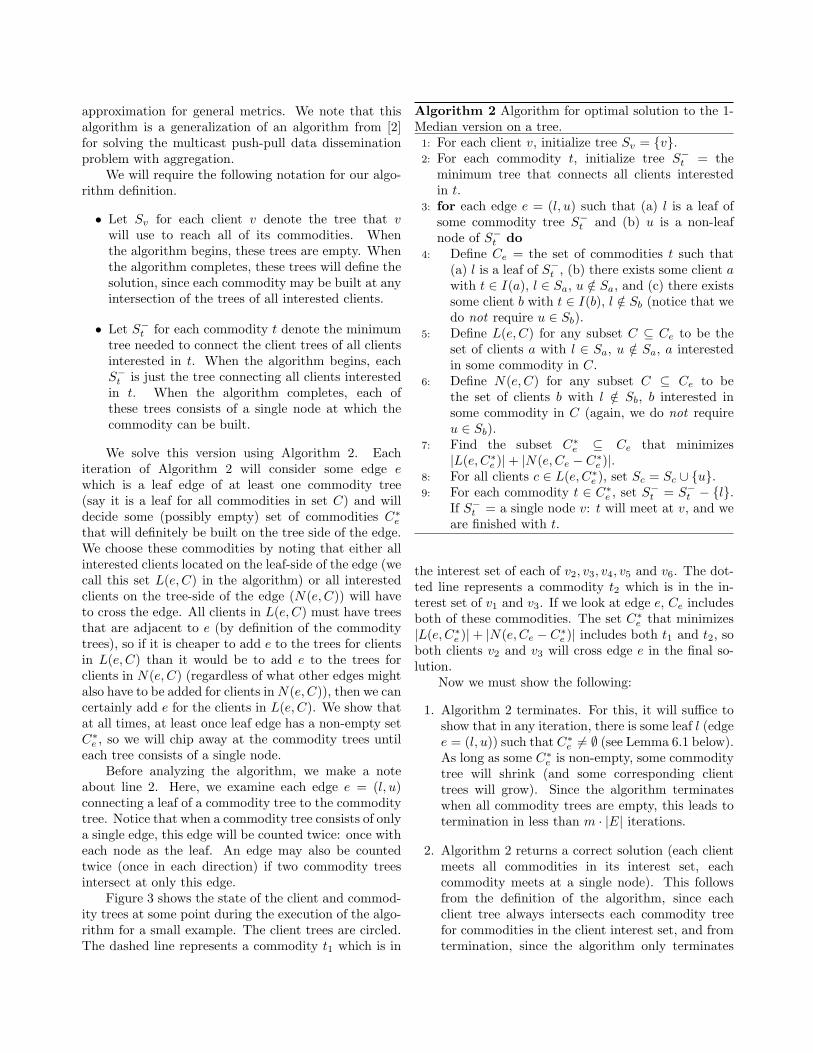
We solve this version using Algorithm 2. Eachiteration of Algorithm 2 will consider some edge ewhich is a leaf edge of at least one commodity tree(say it is a leaf for all commodities in set C) and willdecide some (possibly empty) set of commodities C∗
e
that will definitely be built on the tree side of the edge.We choose these commodities by noting that either allinterested clients located on the leaf-side of the edge (wecall this set L(e, C) in the algorithm) or all interestedclients on the tree-side of the edge (N(e, C)) will haveto cross the edge. All clients in L(e, C) must have treesthat are adjacent to e (by definition of the commoditytrees), so if it is cheaper to add e to the trees for clientsin L(e, C) than it would be to add e to the trees forclients in N(e, C) (regardless of what other edges mightalso have to be added for clients in N(e, C)), then we cancertainly add e for the clients in L(e, C). We show thatat all times, at least once leaf edge has a non-empty setC∗
e , so we will chip away at the commodity trees untileach tree consists of a single node.
Before analyzing the algorithm, we make a noteabout line 2. Here, we examine each edge e = (l, u)connecting a leaf of a commodity tree to the commoditytree. Notice that when a commodity tree consists of onlya single edge, this edge will be counted twice: once witheach node as the leaf. An edge may also be countedtwice (once in each direction) if two commodity treesintersect at only this edge.
Figure 3 shows the state of the client and commod-ity trees at some point during the execution of the algo-rithm for a small example. The client trees are circled.The dashed line represents a commodity t1 which is in
Algorithm 2 Algorithm for optimal solution to the 1-Median version on a tree.1: For each client v, initialize tree Sv = v.2: For each commodity t, initialize tree S−t = the
minimum tree that connects all clients interestedin t.
3: for each edge e = (l, u) such that (a) l is a leaf ofsome commodity tree S−t and (b) u is a non-leafnode of S−t do
4: Define Ce = the set of commodities t such that(a) l is a leaf of S−t , (b) there exists some client awith t ∈ I(a), l ∈ Sa, u /∈ Sa, and (c) there existssome client b with t ∈ I(b), l /∈ Sb (notice that wedo not require u ∈ Sb).
5: Define L(e, C) for any subset C ⊆ Ce to be theset of clients a with l ∈ Sa, u /∈ Sa, a interestedin some commodity in C.
6: Define N(e, C) for any subset C ⊆ Ce to bethe set of clients b with l /∈ Sb, b interested insome commodity in C (again, we do not requireu ∈ Sb).
7: Find the subset C∗e ⊆ Ce that minimizes
|L(e, C∗e )|+ |N(e, Ce − C∗
e )|.8: For all clients c ∈ L(e, C∗
e ), set Sc = Sc ∪ u.9: For each commodity t ∈ C∗
e , set S−t = S−t − l.If S−t = a single node v: t will meet at v, and weare finished with t.
the interest set of each of v2, v3, v4, v5 and v6. The dot-ted line represents a commodity t2 which is in the in-terest set of v1 and v3. If we look at edge e, Ce includesboth of these commodities. The set C∗
e that minimizes|L(e, C∗
e )|+ |N(e, Ce − C∗e )| includes both t1 and t2, so
both clients v2 and v3 will cross edge e in the final so-lution.
Now we must show the following:
1. Algorithm 2 terminates. For this, it will suffice toshow that in any iteration, there is some leaf l (edgee = (l, u)) such that C∗
e 6= ∅ (see Lemma 6.1 below).As long as some C∗
e is non-empty, some commoditytree will shrink (and some corresponding clienttrees will grow). Since the algorithm terminateswhen all commodity trees are empty, this leads totermination in less than m · |E| iterations.
2. Algorithm 2 returns a correct solution (each clientmeets all commodities in its interest set, eachcommodity meets at a single node). This followsfrom the definition of the algorithm, since eachclient tree always intersects each commodity treefor commodities in the client interest set, and fromtermination, since the algorithm only terminates

Figure 3: An example of Algorithm 2. This showsthe state of the client and commodity trees at somepoint during the execution of the algorithm for a smallexample. The client trees are circled. The dashedline represents a commodity t1 which is in the interestset of each of v2, v3, v4, v5 and v6. The dotted linerepresents a commodity t2 which is in the interestset of v1 and v3. If we look at edge e, Ce includesboth of these commodities. The set C∗
e that minimizes|L(e, C∗
e )| + |N(e, Ce − C∗e )| includes both t1 and t2,
so both clients v2 and v3 will cross edge e in the finalsolution.
when each commodity meets at a single node.
3. Algorithm 2 returns an optimal solution. We willshow in Lemma 6.2 that there exists an optimalsolution with the same client trees as those chosenby Algorithm 2.
4. Algorithm 2 can be implemented to run in poly-nomial time. If the algorithm terminates in lessthan m · |E| iterations, and each iteration consistsof finding C∗
e for each of the (at most) 2|E| leafedges (each edge can be a leaf edge twice per it-eration – once in each direction), we only need toshow that we can find C∗
e for an edge e in polyno-mial time. We show this in Lemma 6.3.
Lemma 6.1. Algorithm 2 terminates.
Proof. As stated above, it will suffice to show that inany iteration, there is some leaf l (edge e = (l, u)) suchthat C∗
e 6= ∅.First we will show
(6.4)∑
e=(l,u)
|N(e, Ce)| ≥∑
e=(l,u)
|L(e, Ce)|
where e = (l, u) is an edge connecting a commodity leafto the rest of the commodity tree, as defined in Line 3of Algorithm 2.
Consider how many times an arbitrary client ccontributes to each side of Equation (6.4). c will becounted on the right hand side once for each distinctedge (l1, u1), (l2, u2), . . . (lk, uk) such that li ∈ Sc, ui /∈Sc, li is a leaf of S−ti
for some commodity ti ∈ I(c),ui ∈ S−ti
. We can specify some such commodity ti foredge (li, ui) causing c to appear once on the right handside.
For each of these commodities ti, c will also appearat least once on the left hand side, since each S−ti
musthave at least one other leaf l′i (connected to S−ti
byedge e′i, or else we would have removed ti at Line 9of Algorithm 2. Since ui /∈ Sc, it must also be true thatl′i /∈ Sc, so c will count as part of N(e′, Ce′).
Suppose we have two of these “other leaves” withl′i = l′j (i 6= j). By construction, (li, ui) 6= (lj , uj). Also,l′i ∈ S−ti
, ui ∈ S−ti, l′i = l′j ∈ S−tj
, uj ∈ S−tj, (li, ui) ∈ Sc,
and (lj , uj) ∈ Sc. Now, since S−ti, S−tj
and Sc are alltrees, there exists a cycle from lj across the edge to uj ,then through S−tj
to l′j (= l′i), then through S−tito ui,
along its edge to li, then through Sc back to lj . However,our original graph was a tree, so there cannot be such acycle. Therefore, each client will appear as many timeson the left hand side of Equation (6.4) as on the righthand side, and Equation (6.4) holds.
Because each side of Equation (6.4) contains a sumover all e = (l, u), there must be some such single ewith |N(e, Ce)| ≥ |L(e, Ce)|. For this e, |L(e, ∅)| +|N(e, Ce)| ≥ |L(e, Ce)| + |N(e, ∅)|, so C∗
e (the set thatminimizes |L(e, C∗
e )|+ |N(e, Ce−C∗e )|) is not empty, as
desired.
Lemma 6.2. There exists an optimal solution with theclient trees chosen by Algorithm 2.
Proof. We will prove that there exists an optimal solu-tion whose client trees are supersets of the client treeschosen by Algorithm 2. Clearly, an optimal solutionwill not have trees strictly larger than those chosen byAlgorithm 2, so this is sufficient to prove the lemma.
The proof is by induction on the iterations ofAlgorithm 2. At the start of the algorithm, the clienttrees are empty. Any optimal solution has client treesthat are a superset of empty trees. Now, we will assumethat after some iteration of the algorithm, there is anoptimal solution that includes the partial client treescreated so far by the algorithm, and show that the nextiteration of the algorithm does not add non-optimaledges to the client trees.
Consider any edge e = (l, u) examined in the nextiteration (l is the leaf of a commodity tree S−t , u ∈ S−t ).We have defined set Ce = the set of commodities tsuch that there exists client a with t ∈ I(a), l ∈ Sa,
u /∈ Sa and there exists client b with t ∈ I(b), l /∈ Sb.In any solution, each commodity in Ce must meet onone side or the other of edge e. Suppose there is anoptimal solution such that the commodities in COPT ⊆Ce meet on the u side of e, and the commodities inCe − COPT meet on the l side of e. (In fact, by theinductive assumption and the fact that l is a leaf ofeach commodity in Ce, all commodities in Ce − COPT
meet exactly at l.) If C∗e ⊆ COPT , then our new client
trees are still a subset of the same optimal solution. Soassume C∗
e −COPT 6= ∅. We will show that moving themeeting points of the commodities in C∗
e − COPT froml to u does not increase the cost of the optimal solution.
Before the change to the optimal solution, com-modities in COPT met on the u side of e, those inCe − COPT met on the l side. After the change, com-modities in C∗
e meet on the u side, and those in Ce−C∗e
meet on the l side. The new cost is equal to
optimal cost + d(e)(|L(e, C∗
e )− L(e, COPT )|
(6.5)
− |N(e, Ce − COPT )−N(e, Ce − C∗e )|)
= optimal cost + d(e)(|L(e, C∗
e )|
(6.6)
− |L(e, C∗e ) ∩ L(e, COPT )| − |N(e, Ce − COPT )|
+ |N(e, Ce − COPT ) ∩N(e, Ce − C∗e )|)
= optimal cost + d(e)(|L(e, C∗
e )|
(6.7)
− |L(e, C∗e ) ∩ L(e, COPT )|
− |N(e, Ce − COPT )|+ |N(e, Ce − C∗e )|
− |N(e, Ce − C∗e )−N(e, Ce − COPT )|
)
= optimal cost + d(e)(|L(e, C∗
e )|+ |N(e, Ce − C∗e )|
(6.8)
− |L(e, C∗e ) ∩ L(e, COPT )| − |N(e, Ce − COPT )|
− |N(e, Ce − C∗e )−N(e, Ce − COPT )|
)
≤ optimal cost + d(e)(|L(e, C∗
e )|+ |N(e, Ce − C∗e )|
(6.9)
−(|L(e, C∗
e ∩ COPT )|+ |N(e, Ce − (COPT ∩ C∗e ))|
))
≤ optimal cost(6.10)
Line 6.5 is because we add the cost for clients who haveto cross from l to u to reach commodities in C∗
e butdidn’t have to cross to meet any commodities in COPT ,while we subtract the cost for clients who had to crossfrom u to l to meet commodities in Ce−COPT but don’thave to cross to meet commodities in C − C∗
e .Line 6.6 is true because the set of clients interested
in C∗e but not interested in anything in COPT is the
same as the set of clients interested in C∗e minus the
set of clients interested both in something in C∗e and
in something in COPT (similarly with C − C∗e and
C − COPT ).Line 6.7 is true because the set of clients interested
in something other than C∗e and in something other than
COPT is the same as the set of all clients interestedin something other than C∗
e minus the set of clientsinterested in something other than C∗
e but not insomething other than COPT .
Line 6.8 is just rearranging terms.Line 6.9 is true because the set of clients interested
in commodities in both C∗e and COPT is a subset of the
set of clients interested in some commodity in C∗e and
some commodity in COPT . The set of clients interestedin any commodity not in C∗
e minus the set of clientsinterested in any commodity not in COPT is the sameas the set of clients only interested in commoditiesin COPT but not only interested in commodities inCOPT ∩ C∗
e . Adding this to the set of clients interestedin any commodity not in COPT gives the set of clientsinterested in any commodity in Ce − (COPT ∩ C∗
e ).Finally, Line 6.10 is true because we chose C∗
e asthe set that minimizes |L(e, C∗
e )|+ |N(e, Ce − C∗e )|.
Lemma 6.3. We can find C∗e for an edge e in polyno-
mial time.
Proof. We will solve for an edge e = (l, u) during aniteration by using a directed minimum cut algorithm.Create a directed graph with 5 levels of nodes as follows:Level 1 (source node) = s. Level 2 (tree-side clientnodes) = N(e, Ce). Level 3 (commodity nodes) = Ce.Level 4 (leaf-side client nodes) = L(e, Ce). Level 5 (sinknode) = t.
Let M = max(n, m). There is a directed edge ofweight 1 from s to each node in Level 2, and a directededge of weight 1 from each node in Level 4 to t. There isan edge of weight M +1 from each tree-side client nodeto each commodity node in the client’s interest set, andan edge of weight M + 1 from each commodity node toeach interested leaf-side client node.
The directed min s−t cut of this graph will give theminimum C∗
e . If there is a path from s to a commodity,

it is part of C∗e . If there is a path from the commodity
to t, it is part of Ce − C∗e .
Claim 6.1. A directed min s-t cut of this graph withweight W will give a set C∗
e with |L(e, C∗e )|+ |N(e, Ce−
C∗e )| = W
Proof. In a cut, there will be no paths remaining froms to t. In a min cut, none of the weight M +1 edges willbe cut (since there are at most M nodes in each level).Therefore, W = the number of cut edges s to Level 2 +the number of cut edges Level 4 to t.
We set C∗e = the set of all commodities reachable
from s. Therefore, the edge from each leaf-side client(interested in a commodity in C∗
e ) to t must be part ofthe cut. So we’ve cut one edge for each leaf-side clientinterested in some commodity in C∗
e , which is exactlythe client set L(e, C∗
e ) (by definition of L(e, C∗e )).
Similarly, if there is a path from a commodity to t(the commodity is in Ce − C∗
e ), each edge from s to atree-side client (interested in one of these commodities)must be cut. So we’ve also cut one edge for each tree-side client interested in a commodity in Ce −C∗
e , whichis exactly the client set N(e, Ce − C∗
e ).So the number of edges cut (all of weight 1) is
exactly |L(e, C∗e )|+ |N(e, Ce − C∗
e )|
Claim 6.2. Any C∗e corresponds to a valid directed cut
of this graph with weight = |L(e, C∗e )|+ |N(e, Ce −C∗
e )|
Proof. Given C∗e , cut each edge that goes from s to a
Level 2 node corresponding to a client in N(e, Ce −C∗e )
and cut each Level 4 to t edge corresponding to a clientin L(e, Ce). Now, consider any path from s to t. Itmust pass through the node for some commodity j. Weconsider two cases. The first case is when j ∈ C∗
e . Inthis case, all interested leaf-side clients are in the setL(e, C∗
e ). Therefore, no matter what edge we followfrom the commodity node to a leaf-side client node, theedge from the client node to t has been cut. The secondcase is when j ∈ Ce − C∗
e . In this case, all interestedtree-side clients are in the set N(e, Ce−C∗
e ). Therefore,there are no un-cut edges from s to a tree-side clientnode connected to the commodity. So we have a validcut.
Since we can find a minimum cut in polynomialtime, this concludes the proof of the lemma.
Together, Lemmas 6.1, 6.2, and 6.3 prove thefollowing.
Theorem 6.1. Algorithm 2 is a polynomial time al-gorithm for optimally solving the 1-Median version ofMGSFL.
Although we give an optimal solution on trees, wecan show that the 1-Median version is NP-hard ongeneral metrics via a reduction from Steiner Tree.
Given a Steiner Tree instance, create an MGSFL1-Median instance with the same graph. Create onecommodity tv for each node v to be included in theSteiner tree, and 2 clients located at v, each interestedin only tv. Also add one client c located at theroot, interested in all commodities. Now, consider thelocation of each facility in an optimal MGSFL solution.The cost of the solution will include the path from theroot to each location as well as twice the path lengthfrom each v to the corresponding facility location. Thiscost will naturally be lower if only client c moves, so allcommodities will be built at the Steiner tree locations,and the solution tree for client c will be the minimumSteiner tree.
To approximate the 1-Median version of MGSFLon general metrics, we can use the results from [7] toembed an arbitrary metric into a tree with distortion atmost O(log n). Solving on the resulting tree will give anO(log n) approximation for the metric.
7 Concluding Remarks
There is a gap between the upper and lower boundswe have established for each version of MGSFL. Themajor problem left open by our work is whether apolylogarithmic-approximation ratio is achievable inpolynomial time for general MGSFL; we have achieveda 2O(
√log n log log n) approximation, but the best hardness
result is an Ω(log2−ε m)-factor. The same hardnessbound applies for the version with laminar interest sets,but our ratio O(log4 n log m) is still quite a bit higher.We give an O(log n) approximation for general metricswhen building costs are uniform across locations, but aconstant approximation may be possible. In general, allof our approximations for general metrics incur a cost ofO(log n) factor owing to the reduction to tree metrics;it is unclear whether this gap is inherent. Nevertheless,we have made significant initial progress on this newproblem.
There are other variants that merit study. First,just as we considered laminar constraints on clientinterest sets, the same problem could be defined with“laminar commodities”: given any two commodities,the set of clients interested in them do not intersect orone set of clients is entirely contained in the other. Wehope to be able to reduce general MGSFL into a smallnumber of instances with laminar clients or laminarcommodities. Second, instead of using building costs forcommodities, we could place a bound kt on the numberof facilities that need to be built for each commodityt. The resulting problem is a k-median variant of
MGSFL, an extension of the 1-median variant discussedin Section 6.
References
[1] Vijay Arya, Naveen Garg, Rohit Khandekar, AdamMeyerson, Kamesh Munagala, and Vinayaka Pandit.Local search heuristic for k-median and facility locationproblems. Proceedings of the thirty-third annual ACMsymposium on Theory of computing, pages 21–29, 2001.
[2] R. C. Chakinala, A. Kumarasubramanian, K. A. Laing,R. Manokaran, C. Pandu Rangan, and R. Rajaraman.Playing push vs pull: models and algorithms for dis-seminating dynamic data in networks. Proceedings ofthe eighteenth annual ACM symposium on Parallelismin algorithms and architectures, pages 244–253, 2006.
[3] Moses Charikar, Chandra Chekuri, Ashish Goel, andSudipto Guha. Rounding via trees: deterministic ap-proximation algorithms for group Steiner trees and k-median. Proceedings of the 30th Annual ACM Sympo-sium on Theory of Computing, pages 114–123, 1998.
[4] Moses Charikar, Sudipto Guha, Eva Tardos, andDavid B. Shmoys. A constant-factor approximation al-gorithm for the k-median problem (extended abstract).Proceedings of the thirty-first annual ACM symposiumon Theory of computing, pages 1–10, 1999.
[5] Chandra Chekuri, Guy Even, and Guy Kortsarz. Agreedy approximation algorithm for the group Steinerproblem. Discrete Applied Mathematics, 154(1):15–34,2006.
[6] Fabian Chudak and David B. Shmoys. Improvedapproximation algorithms for a capacitated facilitylocation problem. Proceedings of the tenth annualACM-SIAM symposium on Discrete algorithms, pages875–876, 1999.
[7] Jittat Fakcharoenphol, Satish Rao, and Kunal Talwar.A tight bound on approximating arbitrary metrics bytree metrics. Proceedings of the thirty-fifth annualACM symposium on Theory of computing, pages 448–455, 2003.
[8] Naveen Garg, Goran Konjevod, and R. Ravi. Apolylogarithmic approximation algorithm for the groupSteiner tree problem. Journal of Algorithms, 37(1):66–84, 2000.
[9] Sudipto Guha and Samir Khuller. Greedy strikes back:improved facility location algorithms. Proceedings ofthe ninth annual ACM-SIAM symposium on Discretealgorithms, pages 649–657, 1998.
[10] Eran Halperin, Guy Kortsarz, Robert Krauthgamer,Aravind Srinivasan, and Nan Wang. Integrality ratiofor group Steiner trees and directed Steiner trees. Pro-ceedings of the fourteenth annual ACM-SIAM sympo-sium on Discrete algorithms, pages 275–284, 2003.
[11] Eran Halperin and Robert Krauthgamer. Polyloga-rithmic inapproximability. Proceedings of the thirty-fifth annual ACM symposium on Theory of computing,pages 585–594, 2003.
[12] Ara Hayrapetyan, Chaitanya Swamy, and Eva Tardos.Network design for information networks (extendedabstract). Proceedings of the sixteenth annual ACM-SIAM symposium on Discrete algorithms, pages 933 –942, 2005.
[13] Kamal Jain and Vijay V. Vazirani. Approximationalgorithms for metric facility location and k-Medianproblems using the primal-dual schema and Lagrangianrelaxation. Journal of the ACM (JACM), 48(2):274–296, 2001.
[14] Madhukar R. Korupolu, C. Greg Plaxton, and Rajmo-han Rajaraman. Analysis of a local search heuristic forfacility location problems. Proceedings of the ninth an-nual ACM-SIAM symposium on Discrete algorithms,pages 1–10, 1998.
[15] Mohammad Mahdian, Yinyu Ye, and Jiawei Zhang.Improved approximation algorithms for metric facilitylocation problems. Proceedings of the 5th InternationalWorkshop on Approximation Algorithms for Combina-torial Optimization, pages 229–242, 2002.
[16] Martin Pal, Eva Tardos, and Tom Wexler. Facility lo-cation with nonuniform hard capacities. Proceedingsof the 42nd IEEE symposium on Foundations of Com-puter Science, pages 329–338, 2001.
[17] R. Ravi and A. Sinha. Multicommodity facility lo-cation. Proceedings of the fifteenth annual ACM-SIAM symposium on Discrete algorithms, pages 342–349, 2004.
[18] G. Reich and P. Widmayer. Beyond Steiner’s prob-lem: A VLSI oriented generalization. Proceedings ofthe fifteenth international workshop on Graph-theoreticconcepts in computer science, 411:196–210, 1990.
[19] David B. Shmoys, Eva Tardos, and Karen Aardal.Approximation algorithms for facility location prob-lems (extended abstract). Proceedings of the twenty-ninth annual ACM symposium on Theory of comput-ing, pages 265–274, 1997.