multibody model of a motorbike with a flexible · pdf filemultibody model of a motorbike with...

Multibody Model of a Motorbike with a Flexible Swingarm

Gianni Ferretti1 Bruno Scaglioni2 Andrea Rossi21Politecnico Di Milano, Dipartimento di Elettronica, Informazione e Bioingegneria DEIB

Via Ponzio 34/5, 20133 Milano, Italy2MUSP Lab, Via Tirotti 9, Le Mose, 29122 Piacenza, Italy

Abstract

Considering the specific case of the multibody mod-elling of a racing motorbike, where the rigid model ofthe rear swingarm has been replaced with a flexibleone, a general approach to flexible multibody systemsmodelling in Modelica is presented in this paper. Inparticular, the steps required to generate the model of aflexible body starting from a FEM analysis, performedwith commercial packages, are detailed. Simulationsresults are shown with reference to a sudden brakingand to a series of impacts with curbs. In this last case,an unstable behaviour occurred when considering theflexible component, which is currently under investi-gation.

Keywords: motorcycle dynamics; flexible multibodysystems; finite element method; floating frame of ref-erence; Craig-Bampton method.

1 Introduction

Object-oriented modelling, favoring a real modularand multi-domain approach, has been recognized asa fundamental tool for the mechatronic design, requir-ing an integrated approach to mechanical, electronicand control design [1]. In this respect, even if multi-body dynamics is frequently just one of the physicaldomains involved, the simulation of flexible multibodysystems plays an important role.

On the other hand, in real applications, the task ofmodelling distributed flexibility cannot be addressedwithout the help of finite elements (FE) codes, in or-der to describe complex geometries and material prop-erties. Moreover, for the sake of efficiency of numer-ical simulation, the huge number of nodal coordinatesintroduced by FE modelling, must be reduced to amuch smaller number of modal coordinates, for exam-ple through the classical Craig-Bampton method [2].

Two commercial packages exist that pre-process theoutput of FE codes to get the Modelica model of a

flexible body, one has been developed by the GermanAerospace Center (DLR) [3], the other has been devel-oped by Claytex Services Ltd.

The DLR FlexibleBodies library provides severalModelica classes, namely a flexible beam model(Beam), an annular plate model (AnnularPlate),a thermoelastic plate (ThermoElasticPlate) and amodel for general flexible bodies exported from FEcodes (ModalBody). The results of the FE analy-sis performed by several general purpose codes arefirst processed by another commercial code: FEMBS,implementing modal reduction in a two-step process.Guyan or Craig-Bampton reduction methods are ap-plied in the first step to keep the flexible body input fileto FEMBS small, while in the second step the modes inthe frequency range of interest for multibody simula-tion are selected. The reduced modal representation isthen stored in a Standard Input Data (SID) file [4, 5],an object-oriented data structure developed to definea standard format to exchange data between FE andMBS codes. When a ModalBody class is instantiatedthe user has to specify the name of the SID file con-taining the modal description of the body, which alsostores the original mesh of the FE model, used by Dy-mola to perform the animation of the simulated motionof the flexible body.

The Claytex library generates directly the Model-ica model of a flexible body from the output of themodel reduction process performed by three FE codes:namely Nastran, Genesis and Abaqus.

Object-oriented modelling of general flexible multi-body systems has been also described in [6] (up to theModelica code), based on the parameters of the flex-ible body computed by FEM packages, stored in anASCII file and read by a parsing tool. The model alsomaintains the efficient choice of the generalized coor-dinates implemented in the Modelica standard (rigid)multibody library. Thus, when a body is a componentof a tree structure, the motion of the local FloatingFrame of Reference (FFR) [7] is actually calculated by

DOI10.3384/ECP14096273

Proceedings of the 10th International ModelicaConferenceMarch 10-12, 2014, Lund, Sweden

273

propagating of the kinematic quantities from the rootof the tree while, in the case of floating bodies, thebody itself is a root, introducing its own generalizedcoordinates for position and orientation.

In this paper, the above mentioned approach is ap-plied to the multibody model of a racing motorbike,where a flexible model of the rear swingarm has beenconsidered.

First, a rigid multibody model of the motorbike hasbeen developed, with the aim of providing forces andtorques applied to the frame and to the swingarm for afollowing FEM structural analysis, performed for thesake of mechanical design validation. As referencesimulation scenarios a sudden braking and a series ofimpacts with obstacles (curbs) have been considered.Then, the rigid model of the rear swingarm has beenreplaced with a flexible one and the simulation resultshave been compared.

In view of the particular simulation experimentsconsidered only limited differences were expected,particularly appreciable during the simulation of im-pacts. On the other hand, the simulation of the mo-torbike with a flexible swingarm showed an unstablebehaviour in the case of subsequent impacts, largelydue to a poor performance of the virtual driver, but un-doubtedly induced by swingarm flexibility, since thesaid behaviour in the rigid case did not occur.

The paper is organized as follows. In Section 2 therigid multibody model of the motorbike is described,including the simulation scenarios and the related re-sults, moreover, the simulation results are compared toexperimental results obtained on the real bike. Section3 explains the flexible multibody modelling approachused in this paper, describing the adopted theoreticalformulation and the most relevant characteristics of theModelica flexible body model. Further, it describes theprocedure which leads to obtain flexible body modelsin Modelica. In Section 4 the flexible model of the rearswingarm is described, the procedure outlined in theprevious section is adopted to obtain a flexible modelof the body, then, in Section 5 the previously describedsimulations are repeated and the results are comparedwith respect to the rigid model. Section 6 concludesthe paper.

2 Rigid multibody motorbike model

A rigid multibody model of a racing motorbike, builtby RobbyMoto Engineering S.r.L., has been first de-veloped (Fig. 1).

Since the considered scenarios were a sudden brak-

Figure 1: Model of the motorbike.

Figure 2: Scheme of the Modelica model of the mo-torbike.

ing and a series of impacts with obstacles (curbs), themodel was not intended to simulate the dynamic be-haviour of the motorbike in curves, but a steering de-gree of freedom was anyway provided, in order to rep-resent the intrinsically unstable behaviour of the ve-hicle. The adopted tyre model accounted for lateralforces and roll angle, thus a tilt control was required.

The rigid motorbike model is made up entirely bycomponents of the standard Modelica multibody li-brary, except for the wheel/road interaction model andthe virtual driver, taken from [8, 9]. The main compo-nents are:

• Main frame,

• Front suspensions,

• Rear suspended Pro-Link swingarm,

• Wheels and wheel-road interaction,

• Virtual driver: a simple vehicle stabilizer, actingon the front steer and controlling the tilt angle.

and the scheme of the Modelica model is shown inFig. 2.


274 Proceedings of the 10th International ModelicaConferenceMarch 10-12, 2014, Lund, Sweden

DOI10.3384/ECP14096273

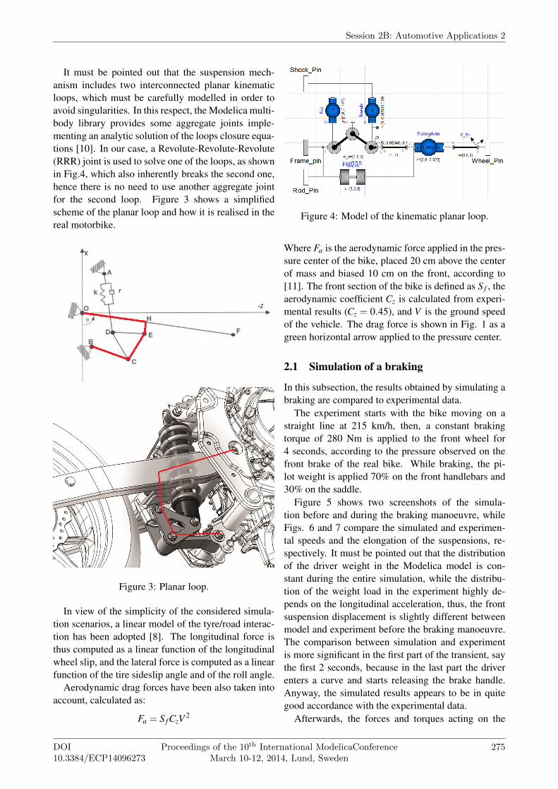
It must be pointed out that the suspension mech-anism includes two interconnected planar kinematicloops, which must be carefully modelled in order toavoid singularities. In this respect, the Modelica multi-body library provides some aggregate joints imple-menting an analytic solution of the loops closure equa-tions [10]. In our case, a Revolute-Revolute-Revolute(RRR) joint is used to solve one of the loops, as shownin Fig.4, which also inherently breaks the second one,hence there is no need to use another aggregate jointfor the second loop. Figure 3 shows a simplifiedscheme of the planar loop and how it is realised in thereal motorbike.

Figure 3: Planar loop.

In view of the simplicity of the considered simula-tion scenarios, a linear model of the tyre/road interac-tion has been adopted [8]. The longitudinal force isthus computed as a linear function of the longitudinalwheel slip, and the lateral force is computed as a linearfunction of the tire sideslip angle and of the roll angle.

Aerodynamic drag forces have been also taken intoaccount, calculated as:

Fa = S fCzV 2

Figure 4: Model of the kinematic planar loop.

Where Fa is the aerodynamic force applied in the pres-sure center of the bike, placed 20 cm above the centerof mass and biased 10 cm on the front, according to[11]. The front section of the bike is defined as S f , theaerodynamic coefficient Cz is calculated from experi-mental results (Cz = 0.45), and V is the ground speedof the vehicle. The drag force is shown in Fig. 1 as agreen horizontal arrow applied to the pressure center.

2.1 Simulation of a braking

In this subsection, the results obtained by simulating abraking are compared to experimental data.

The experiment starts with the bike moving on astraight line at 215 km/h, then, a constant brakingtorque of 280 Nm is applied to the front wheel for4 seconds, according to the pressure observed on thefront brake of the real bike. While braking, the pi-lot weight is applied 70% on the front handlebars and30% on the saddle.

Figure 5 shows two screenshots of the simula-tion before and during the braking manoeuvre, whileFigs. 6 and 7 compare the simulated and experimen-tal speeds and the elongation of the suspensions, re-spectively. It must be pointed out that the distributionof the driver weight in the Modelica model is con-stant during the entire simulation, while the distribu-tion of the weight load in the experiment highly de-pends on the longitudinal acceleration, thus, the frontsuspension displacement is slightly different betweenmodel and experiment before the braking manoeuvre.The comparison between simulation and experimentis more significant in the first part of the transient, saythe first 2 seconds, because in the last part the driverenters a curve and starts releasing the brake handle.Anyway, the simulated results appears to be in quitegood accordance with the experimental data.

Afterwards, the forces and torques acting on the

Session 2B: Automotive Applications 2

DOI10.3384/ECP14096273


275

Figure 5: Screenshots of the simulation before andduring the braking.

frame and rear swingarm (Fig. 8) have been recordedfrom the simulation, in order to identify the stress peakand the actual values of loads to be used during a FEManalysis.

2.2 Impacts with curbs

In a second simulation experiment a series of impactswith curbs has been considered.

Curbs have been modeled as sawtooth obstacles(Fig. 9) placed on the road surface, every sawtooth hasan height of 2 cm and a width of 20 cm, in order to re-produce the real curbs of most racetracks. To this aim,the road model described in [8] has been modified inorder compute the quote of the road, given the positionof the wheel. Since the driver weight distribution wasimpossible to estimate in this experiment, the wholeload (70 kg) was placed on the saddle. The forces andtorques acting on the frame and rear swingarm havebeen exported for a following FEM analysis step, Fig.10 shows vertical forces exchanged between rear armand main frame in the hinge.

Figure 6: Speeds during braking.

Figure 7: Front and rear suspension elongation duringbraking.

3 Flexible multibody modelling inModelica

The object-oriented modelling paradigm implementedby the Modelica language requires a description of thedynamics of a flexible body in terms of local vari-ables, while the interaction between different bodieshas to be described using the connectors of the stan-dard Modelica multibody library [10]. In turn, a localdescription of a body’s dynamics naturally calls for afloating frame of reference (FFR) approach [7], whichis currently the most widely used method in computersimulation of flexible multibody systems.

In the FFR formulation, each body is attached toa moving frame of reference undergoing large (rigid)motion, while the (small) elastic displacements are ob-tained in local coordinates with respect to the referenceframe. Thus, the position (in local coordinates) of apoint on a flexible body, see Fig. 11, is given by:

u = u0 + u f , (1)

where u0 is the “undeformed” (i.e., rigid) position vec-tor and u f is the deformation contribution to position(i.e., the deformation field).

If small elastic deflections are considered, accord-ing to the classical Rayleigh-Ritz method [12], the in-finite dimensional deformation field on the body can



DOI10.3384/ECP14096273

Figure 8: Forces acting on the rear swingarm hingeduring braking.

Figure 9: Curbs model.

be approximated by a functional basis space with fi-nite dimension, say M, so that the vector u f can beexpressed by the finite dimensional product

u f = Sq , (2)

where S is the [3×M] shape functions matrix (i.e., amatrix of functions defined over the body domain andused as a basis to describe the deformation field of thebody itself) and q is the M-dimensional vector of de-formation degrees of freedom, or modal coordinates.The representation of a generic flexible body in theworld reference frame requires then 6 + M d.o.f.: 3corresponding to the rigid displacements r, 3 to theundeformed body orientation angles θ and M to themodal coordinates q.

Starting from eqs. (1,2) and accounting for the elas-tic properties of the material and for the mass distri-bution, the generalized Newton-Euler equations for ageneric unconstrained flexible body, formulated withrespect to the FFR, can be derived in [13, 7, 14, 15, 5,16], and developed up to the Modelica code in [6]. Itmust be also pointed out that the efficient choice of thegeneralized coordinates, implemented in the Modelicastandard (rigid) multibody library, can be maintained.Thus, when a body is a component of a tree structure,the motion of the FFR is actually calculated by propa-gation of the kinematic quantities from the root of thetree while, in the case of floating bodies, the body itselfis a root, introducing its own generalized coordinatesfor position and orientation.

Figure 10: Vertical forces acting on the rear swingarmhinge during impacts with curbs.

Figure 11: Floating reference frame.

In the case of simple geometries, such as beams[13], the set of data required to implement the flexi-ble body dynamic equations, summarized in Table 1,can be determined analytically, but in more generalcases the use of finite elements (FE) computer codesas preprocessors is necessary. In this last case thehuge number of nodal coordinates must be reduced toa much smaller number of modal coordinates, throughthe classical Craig-Bampton method [2] or other re-cently proposed methods [17, 18, 14, 19].

The Modelica model of a general flexible body:FEMBody, is characterized by an array of Nc multibodyconnectors, while the data in Table 1 have been suit-ably collected in the Modelica record BodyData. Therecord is defined as replaceable:

replaceable parameter FEMData.BodyData

data;

so that it is possible, by exploiting the features of theModelica language, to assign a different data record toeach FEMBody instance, by simply replacing the recordin the model declaration:

FEMBody FlexPendulum(redeclare

FEMData.PendulumData data ,

alpha=0.005 ,


DOI10.3384/ECP14096273


277

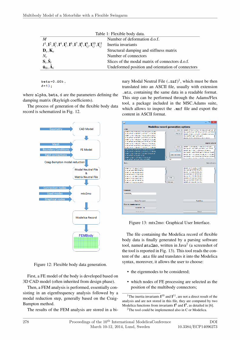
Table 1: Flexible body data.M Number of deformation d.o.f.I1,I2,I3

i ,I4,I5i ,I6,I7,I8

i ,I9i j,I10

i j ,I11i j Inertia invariants

De,Ke Structural damping and stiffness matrixNc Number of connectorsSi, Si Slices of the modal matrix of connectors d.o.f.u0i, Ai Undeformed position and orientation of connectors

beta=0.005 ,

d=1);

where alpha, beta, d are the parameters defining thedamping matrix (Rayleigh coefficients).

The process of generation of the flexible body datarecord is schematized in Fig. 12.

Figure 12: Flexible body data generation.

First, a FE model of the body is developed based on3D CAD model (often inherited from design phase).

Then, a FEM analysis is performed, essentially con-sisting in an eigenfrequency analysis followed by amodal reduction step, generally based on the Craig-Bampton method.

The results of the FEM analysis are stored in a bi-

nary Modal Neutral File (.mnf)1, which must be thentranslated into an ASCII file, usually with extension.mtx, containing the same data in a readable format.This step can be performed through the Adams/Flextool, a package included in the MSC.Adams suite,which allows to inspect the .mnf file and export thecontent in ASCII format.

Figure 13: mtx2mo: Graphical User Interface.

The file containing the Modelica record of flexiblebody data is finally generated by a parsing softwaretool, named mtx2mo, written in Java2 (a screenshot ofthe tool is reported in Fig. 13). This tool reads the con-tent of the .mtx file and translates it into the Modelicasyntax, moreover, it allows the user to choose:

• the eigenmodes to be considered;

• which nodes of FE processing are selected as theposition of the multibody connectors;

1The inertia invariants I10 and I11, are not a direct result of theanalysis and are not stored in this file, they are computed by twoModelica functions from invariants I8 and I9, as detailed in [6].

2The tool could be implemented also in C or Modelica.



DOI10.3384/ECP14096273

• how many FE nodes are selected for the 3Dgraphic rendering of the model.

The described approach thus avoids the preprocess-ing stage adopted by the DLR FlexibleBodies library,which requires the models to be processed by FEMBSin order to obtain the SID file.

Figure 14: FE model of the swingarm.

4 Modelling a flexible swingarm

Figure 14 shows the FE model of the swingarm, re-alised with the Patran/Nastran suite by MSC.Software.

Figure 15: Multi-point constraint.

The swingarm is characterized by three connectionpoints, so three virtual nodes have been defined in theFE geometry: one in the center of the frame pivot, onein the lower triangle pivot, and one in the center of thewheel hub. The internal surfaces of bores have beenassociated to this massless nodes by RBE2 rigid multi-point connections, namely, every node of the mesh lo-cated on the surface of the holes is rigidly connectedto the virtual node, so that the motion of all dependentnodes is constrained by the motion of one node. Fig-ure 15 shows the rigid connection between nodes inthe front bore.

The boundary conditions were assigned in order toreproduce the hinge acting on the rear swingarm: alltranslations and two rotations were fixed for the pin

connecting the swingarm to the mainframe, while allthe other nodes were free to move. A free-motioneigenvalue resulted from the FEM analysis, with avery small absolute value (1.2 ·10−3 Hz), neglected inthe generation of the Modelica model.

The first 20 eigenmodes were retained from theFEM analysis, with eigenfrequencies ranging from117.3 Hz to 3585.6 Hz, the first eigenmode is shownin Fig. 16.

Figure 16: First torsional eigenmode.

It must be pointed out that structural damping is ac-counted in the flexible body model by means of theRayleigh coefficients, which are difficult to estimateand are often the result of an averaging on the dampingratios of different modes. In this work the coefficientsare chosen as d = 1,α = β = 0.005.

The Modelica model of the flexible swingarm isshown in Fig. 17. Note that, for the sake of modu-larity, the connectors of the flexible body are storedin a vector, hence it is not possible to distinguish theconnections in the graphical layer of the model.

It must be also pointed out that the RRR joint usedin the rigid case to manage the kinematic loop is nolonger required, as the flexibility of the body inher-ently breaks the loop.

A relative position sensor has been also introduced,with the aim of sensing the deflection of the rear wheelhub with respect to the position of the rear wheel borein the undeformed configuration.

Figure 17: Modelica model of flexible swingarm.


DOI10.3384/ECP14096273


279

5 Simulation results with a flexibleswingarm

Figure 18: Displacement of rear wheel hub in braking.

Figure 19: Vertical position of vehicle mass center dur-ing braking.

The experiments reported in Section 2 have been re-peated with the flexible swingarm model.

Figure 18 shows the deflection of the rear hub mea-sured by the above mentioned relative sensor. Dur-ing the braking manoeuvre the swingarm deflects un-der the load on the rear part of the bike, starting froma value of 0.16 mm on the vertical axis before brak-ing. A lateral displacement is also measured, due tothe imprecise virtual driver, which cannot mantain themotorbike perfectly vertical. Although the swingarmdeflection is small, it anyway affects the overall geom-etry of the vehichle.

In Fig.19 the quotes of the mass center of the over-all vechicle are shown, in the rigid and flexible case.During the braking, the weight and the inertia loadsmainly impact on the front wheel, while the rear sus-pension reaches an equilibrium where poor forces areapplied.

Forces and torques applied on the frame do notchange significantly with respect to the rigid model,in Fig. 20 the vertical forces in the rear hinge arecompared between the rigid and the flexible case atthe beginning of the manoeuvre. As expected, the dif-

ferences (≈3% of the maximum value) are scarcelyappreciable in the transients, and the deformation val-ues are in good accordance with the static FE analysis(Fig. 21), in which the same loads (extracted from themultibody analysis) are applied.

Figure 20: Vertical forces at the beginning of brakingmanoeuvre.

Figure 21: FEM static analisys of rear arm displace-ment.

During the simulated impacts with curbs the forcesacting on the wheel, and consequently on the rear arm,are much higher in magnitude. Figure 22 shows thedeflection of the rear wheel hub when the motorbikefaces curbs. Note that in this case the vertical deflec-tion reaches values up to 0.6 mm.

Figure 23 shows a comparison between the verticalforces in the rear hinge in the rigid and flexible case.As expected, the forces in the flexible case are lowerin absolute value, because part of the energy is usedto deform the flexible component, which shows also adissipative behaviour due to damping.

The overall behaviour of the motorbike in this casechanges significantly due to flexibility, Fig.24 showsa comparison of the mass center quote of the motor-bike in rigid and flexible case, the differences reachan absolute value of 10 mm. Moreover, when consid-ering the flexible swingarm, an interesting behaviourappears.

If the simulation time is long enough, the virtualdriver is no more able to control the vehicle, whichstarts to wave after some seconds. Figure 25 shows



DOI10.3384/ECP14096273

the motorbike pose in both cases (flexible on the leftand rigid on the right) at time t = 5.5 s: the vehiclewith a flexible swingarm comes into an unstable be-haviour and is going to thumble. This behaviour, cur-rently under investigation, is certainly due to a poorperformance of the virtual driver and to a rough modelof the tyres, but appears to be induced by swingarmflexibility.

Figure 22: Vertical and longitudinal displacement ofrear hub when facing curbs.

Figure 23: Vertical forces in rear hinge, comparisonbetween rigid and flexible case.

The main drawback of model with the flexible com-ponent is the computational cost due to the additionalelastic degrees of freedom: the braking simulation ex-periment with a rigid swingarm takes 0.32 s of CPUtime to simulate 7 s, on a normal laptop, the samemodel with a flexible swingarm takes about 10.4 sec-onds of CPU time; regarding the simulation of im-pacts, the rigid model takes 5 s while the flexiblemodel takes 64 s for 3.5 s of simulated time. TheDASSL integration algorithm has been used in all thesimulations.

6 Conclusion and future work

In this paper, a Modelica multibody model of a motor-cycle with a flexible swingarm is presented.

Figure 24: Mass center quote, comparison betweenrigid and flexible case.

Figure 25: Motorbikes with rigid (right) and flexible(left) swingarm at time t = 5.5 s.

At first, a rigid model of the motorbike has been de-veloped and validated with respect to a sudden brakingtransient.

Then, a general approach to the modelling of flexi-ble bodies is presented, and the full procedure leadingto the Modelica model is detailed.

The proposed modelling approach has been appliedto the rear swingarm of the motorbike and a compar-ison between the rigid and the flexible case is pre-sented, with reference to a sudden braking and a seriesof impacts with curbs as simulation scenarios. In par-ticular, the simulation of the motorbike with a flexibleswingarm showed an unstable behaviour in the caseof subsequent impacts, largely due to a poor perfor-mance of the virtual driver, but undoubtedly inducedby swingarm flexibility.

The developed approach to flexible multibody mod-elling will allow to easily include the description ofbodies’ flexibility in mechatronic systems, expandingthe range of the dynamic analysis. In particular, thesaid unstable behaviour is currently under investiga-tion, as well as another unstable behaviour (shimmy)occurring in racing bikes.


DOI10.3384/ECP14096273


281

7 Acknowledgements

The authors would like to thank all people who sup-ported this work: Dr. Marta Massera, for designingthe frame and the swingarm, the Director of MUSP,prof. Michele Monno, and its staff for constant sup-port, and RobbyMoto Engineering S.r.L., for valuablecollaboration.

References

[1] G. Ferretti, G. Magnani, P. Rocco, Virtual pro-totyping of mechatronic systems, IFAC JournalAnnual Reviews in Control 28 (2) (2004) 193–206.

[2] R. R. Craig, M. C. C. Bampton, Coupling of sub-structures for dynamic analyses, AIAA Journal6 (7) (1968) 1313–1319.

[3] A. Heckmann, M. Otter, S. Dietz, J. D. López,The DLR FlexibleBodies library to model largemotions of beams and of exible bodies exportedfrom nite element programs, in: 5th ModelicaConference, Vienna, Austria, 2006, pp. 85–95.

[4] O. Wallrapp, Standardization of flexible bodymodeling in multibody system codes, Part I: Def-inition of Standard Input Data, Mechanics BasedDesign of Structures and Machines 22 (3) (1994)283 – 304.

[5] R. Schwertassek, O. Wallrapp, A. A. Shabana,Flexible multibody simulation and choice ofshape functions, Nonlinear Dynamics 20 (1999)361–380.

[6] G. Ferretti, A. Leva, B. Scaglioni, Object-oriented modelling of general flexible multibodysystems, Mathematical and Computer Modellingof Dynamical Systems 20 (1) (2014) 1–22.

[7] A. A. Shabana, Dynamics of Multibody Systems,Cambridge University Press, 1998.

[8] F. Donida, G. Ferretti, S. M. Savaresi, M. Tanelli,Object-oriented modelling and simulation of amotorcycle, Mathematical and Computer Mod-elling of Dynamical Systems 14 (2) (2008) 79–100.

[9] Marescotti, L., Modellazione dei sistema pilota-veicolo a due ruote in ambiente integrato Matlab-Adams (in Italian), Master’s thesis, Universitï¿½di Pisa (2003).

[10] M. Otter, H. Elmqvist, S. Mattsson, The newModelica multibody library, in: 3rd ModelicaConference, Linköping, Sweden, 2003.

[11] G. Cocco, Dinamica e tecnica della motocicletta,2013.

[12] W. Ritz, Über eine neue Methode zur Lö-sung gewisser Variationsprobleme der mathema-tischen Physik, Journal für die Reine und Ange-wandte Mathematik 135 (1909) 1–61.

[13] F. Schiavo, L. Viganò, G. Ferretti, Object-oriented modelling of flexible beams, MultibodySystem Dynamics 15 (3) (2006) 263 – 286.

[14] J. Fehr, P. Eberhard, Simulation process of flex-ible multibody systems with non–modal modelorder reduction techniques, Multibody SystemDynamics 25 (2011) 313–334.

[15] U. Lugrís, M. A. Naya, A. Luaces, J. Cuadrado,Efficient calculation of the inertia terms in float-ing frame of reference formulations for flexiblemultibody dynamics, Proceedings of the Institu-tion of Mechanical Engineers, Part K: Journal ofMulti-body Dynamics 223 (2) (2009) 147–157.

[16] R. Schwertassek, O. Wallrapp, Dynamik flex-ibler Mehrkörpersysteme, Vieweg, Wiesbaden,1999.

[17] P. Koutsovasilis, M. Beitelschmidt, Comparisonof model reduction techniques for large mechani-cal systems, Multibody System Dynamics 20 (2)(2008) 111–128.

[18] M. Lehner, P. Eberhard, A two-step approach formodel reduction in flexible multibody dynam-ics, Multibody System Dynamics 17 (2007) 157–176.

[19] C. Nowakowski, J. Fehr, M. Fischer, P. Eberhard,Model order reduction in elastic multibody sys-tems using the floating frame of reference formu-lation, in: 7th Vienna International Conferenceon Mathematical Modelling - MATHMOD 2012,Vienna, Austria, 2012.



DOI10.3384/ECP14096273

multibody model of a motorbike with a flexible · pdf filemultibody model of a motorbike with...

Documents