multi-objective unit commitment with introduction of a methodology for probabilistic assessment of...

Multi-objective unit commitment with introduction of a methodologyfor probabilistic assessment of generating capacities availability

Blaže Gjorgiev a,n, Duško Kančev a, Marko Čepin b, Andrija Volkanovski a

a Reactor Engineering Division, Jožef Stefan Institute, Jamova 39, SI-1000 Ljubljana, Sloveniab Faculty of Electrical Engineering, University of Ljubljana, Tržaška 25, SI-1000 Ljubljana, Slovenia

a r t i c l e i n f o

Article history:Received 19 April 2014Received in revised form6 July 2014Accepted 18 September 2014

Keywords:Unit commitmentGeneration dispatchPower systemUnavailabilityGenetic algorithmMulti-objective optimization

a b s t r a c t

The goal of the short-term unit commitment is the minimization of the total operation cost whilesatisfying all unit and system constraints. One of the main issues while solving the unit commitmentoptimization problem is the planning of the capacity reserves of the power system. In order to addressthis issue, a dynamic method for probabilistic assessment of generation unavailability is proposed withinthis paper. The main highlight feature of this method is that it has the capacity to account for theunavailability implications of the generating unit states, being committed or decommitted as well astheir start-up characteristics. This allows more comprehensive hour-to-hour scheduling analyses fromthe aspect of probabilistic unavailability assessment. The generating capacities unavailability isdesignated as the relevant unavailability measure regarding the power supply to loads. The unitcommitment problem is developed as a multi-objective optimization problem. Two objective functionsare considered: the total operating cost of the generating capacities as one and generating capacitiesunavailability as the other objective function. An improved hybrid genetic algorithm is applied forsolving the problem. A test power system is used as a case study. The obtained results indicate the needand benefits of more detailed modelling of the power generation availability.

& 2014 Elsevier Ltd. All rights reserved.

1. Introduction

The general idea behind the short-term unit commitment (UC)is meeting the forecasted load on a short-term basis (one day or upto one week) by accordingly scheduling the on or off line status ofthe generating capacities (Cheng et al., 2002). The objective of theshort-term UC is the minimization of the total operation costwhile satisfying all unit and system constraints. The UC problem ishighly constrained, non-linear, mixed integer optimization pro-blem. The exact solution of the problem can be obtained bycomplete enumeration, a process which is not computationallyfeasible for realistic power systems (Orero and Irving, 1997; Woodand Wollenberg, 1996).

Modern meta-heuristic algorithm based techniques have beenextensively employed for solving generation scheduling problems.One of the first applications of genetic algorithm (GA) on thegeneration (economic) dispatch optimization problem is shown inRef. Walters and Sheble (1993). Approximately in the same periodthe simulated annealing (SA) algorithm was also applied for theoptimal generation dispatching (Wong and Fung, 1993). Since then

various modern techniques have been used for the single objectiveand multi-objective generation dispatch problem. In Ref. Elsayedet al. (2014) a new GA has been proposed for solving engineeringproblems including optimal generation dispatching. A modifiedparticle swarm optimization has been used on the static genera-tion dispatch problem considering valve point-effects and prohib-ited operating zones (Neyestani et al., 2010). Ref. Lu et al. (2011)introduces three novel chaotic differential evolution techniques forsolving the dynamic generation dispatch problem.

UC problem is another part of the generation scheduling thatwas solved with modern meta-heuristic algorithms. Since begin-ning of the 1990s, when the GAs were first employed in powersystem optimization, they have become very popular tool forsolving the UC problem. In Ref. Dasgupta and McGregor (1994)the application of a binary coded GA has been discussed forsolving the UC problem. Similar study was presented in Ref.Kazarlis et al. (1996) where Kazarlis et al. applied a binary codedGA on a 10-unit test system. The results in this study are comparedwith classical techniques such as dynamic programming (DP) andLagrange relaxation (LR). Later on, the application of a real codedGA for the UC problem was discussed (Damousis et al., 2004).It was shown that real coded GA can produce better results thanthe LR method that was used as a benchmark in the paper, also theexecution time of the algorithm was reduced compared to thebinary coded GA. Other modern meta-heuristic techniques have

Contents lists available at ScienceDirect

journal homepage: www.elsevier.com/locate/engappai

Engineering Applications of Artificial Intelligence

http://dx.doi.org/10.1016/j.engappai.2014.09.0140952-1976/& 2014 Elsevier Ltd. All rights reserved.

n Corresponding author. Tel.:þ386 1 5885 284; fax:þ386 1 5885 377.E-mail addresses: [email protected] (B. Gjorgiev),

[email protected] (D. Kančev), [email protected] (M. Čepin),[email protected] (A. Volkanovski).

Engineering Applications of Artificial Intelligence 37 (2015) 236–249

www.sciencedirect.com/science/journal/09521976

www.elsevier.com/locate/engappai

http://dx.doi.org/10.1016/j.engappai.2014.09.014



http://crossmark.crossref.org/dialog/?doi=10.1016/j.engappai.2014.09.014&domain=pdf



mailto:[email protected]





been extensively used for the UC problem as well, such as:evolutionary programming (Juste et al., 1999), neural networks(Ouyang and Shahidehpour, 1992), simulated annealing (Mantawyet al., 1998), particle swarm optimization (Ting et al., 2006), antcolony (Simon et al., 2006) and artificial bee colony algorithm(Chandrasekaran et al., 2012).

A careful planning of the reserves is required in the short-termUC schedule in order to ensure an adequate reliability level. Eventhough most of the above-mentioned techniques offer an accep-table solution for the UC problem, they are using old and mostcommonly used methods for reserve planning, i.e. low margin as apercentage from the real system load at each time interval and thereserve equal to the power output of one or more of the largestunits. These methods can lead to overscheduling which meansmore reliable and uneconomic unit commitment as well as under-scheduling which means more economic and less reliable unitcommitment. However, some studies, where probabilistic reserveevaluation is used, have been performed. Dillon et al. presented aprobabilistic method for proper representation of the reservesassociated with different unavailability levels (Dillon et al., 1978).The developed model is integrated within the short-term UC asconstraint that has to be satisfied. This model ensures that a givenreliability level is achieved. Similar approach is used in Ref.Shi et al. (2004) where a stochastic mechanism is developedfor the short-term UC with probabilistic determination forspinning reserve constraint. In Ref. Lee and Chen (2007) amethod for solving the short-term UC problem with probabilisticreserves is discussed. In Ref. Simopoulos et al. (2006) evaluation ofthe required spinning reserve capacity is performed by applyingreliability constraints based on loss of load probability (LOLP) andexpected energy not supplied (EENS) indices. Similar approach ispresented in Ref. Jalilzadeh et al. (2009) where a dynamic penaltyconstraint is applied for the EENS constraint. A two-level, two-objective optimization scheme based on evolutionary algorithmsfor solving UC problem by considering stochastic power demandvariations is proposed in Ref. Georgopoulou and Giannakoglou(2009). The total operating cost is used as one objective while therisk of not fulfilling possible demand variations is used as thesecond objective to be minimized. In other words the paperinvestigates the trade-off between total cost and the risk due toload uncertainties. In Ref. Lei et al. (2008) the loss of loadexpectation (LOLE) is included as a constraint in the long-termUC for calculating the cost of supplying the reserve. In Ref.Bouffard and Galiana (2004) an algorithm is developed thatincludes the scheduling of spinning reserve according to a hybriddeterministic/probabilistic reliability criterion. This hybrid criter-ion behaves consistently with purely probabilistic criteria such asLOLP. In most of these methods an optimal reserve planning isachieved when a probabilistically determined generating reserveis used as controlled criteria/constraint, instead of an independentobjective function. Additionally, most of these techniques do notaccount for the implications for unavailability of the commitmentof a specific unit at given time interval and the time needed forthese units (rapid-starting, slow-starting) to be online and startgenerating. These are the main motivations for the work done inthis study.

The increased reliability of power supply corresponds toincreased costs (Billinton and Allan, 1988). The same rationale isvalid for the short-term unit commitment. This research is focusedon the interdependence between the total cost of power produc-tion, the capacity outage unavailability and generation reserves inthe short-term UC. The main objective of this study is to develop adynamic method for power system probabilistic unavailabilityevaluation. The generating capacities unavailability is the relevantunavailability measure. As such, the LOLP is used as an unavail-ability index herein. This approach has the capacity to account for

the time inertia related to different generating units to be onlineand start generating. The second objective of the paper is perform-ing trade-off analysis between the total production costs and thecapacity outage unavailability. Therefore, the UC is presented as amulti-objective optimization problem. For comparative purposes adeterministic model is introduced as well. This deterministicmodel is defined as a function of the spinning reserve.

For solving the short-term UC optimization problem animproved hybrid GA is constructed. The algorithm uses classicalmethod, i.e. priority list in order to create the initial population.An improvement of the classical hybrid GA (Orero and Irving, 1997) isproposed by employing hybrid solutions additionally within theinitial population. The algorithm employs repairing mechanismsand penalization technique to deal with the constraint violations.The UC problem is solved in three separate formulations. Firstly, theproblem is solved as a single objective, once considering the totalproduction cost objective function and secondly, considering thegeneration unavailability function. At the end, the problem is solvedas a bi-objective, considering both of the objective functions. Twoscenarios are analysed: considering and not considering the spinningreserve constraint. The obtained results show that compromisebetween cost and unavailability is achieved. Additionally, improve-ments on the used test power system are proposed and the systemas such is solved using the same model. For verification purposes, theused algorithm has been applied on a 10, 20, 40, 60, 80 and 100 unitsystems and the obtained results were compared with othersavailable in the literature.

2. Power system reliability

The primary objectives of the modern power systems are toprovide a reliable and economic supply of electric energy to theircustomers. The main issue in the planning and also in theoperating phases has always been the adequate reserves ofgenerating capacity. Consequently, the level of redundancy andthe associated cost are designated as the prime question. Bydefinition, the reserve capacities that are spinning, synchronizedand ready to take up load are known as spinning reserve. Somepower system operators include only the spinning reserve in theassessment of system adequacy, while others include also therapid start units such as gas turbines and hydropower plants orassistance from the interconnected systems. These additionalfactors added to the spinning reserve are all together known asoperating reserve (Billinton and Allan, 1996). The operating capa-city domain, i.e. the short-term unit commitment is of interest inthis research paper.

In general, each power system operation is associated withprediction of the expected load, i.e. short-term load forecasting,and consequently providing for and scheduling of sufficient gen-eration capacity. The time needed for a specific generating unit toproduce an output ranges from few minutes in the case of gasturbines and hydropower plants to several hours in the case ofthermal generating power plants. This is especially important forthe intermediate load units which are mostly coal-fired units thathave considerable starting inertia (several hours). If an unexpectedchange occurs in the power system and additional generation isrequired immediately, the intermediate load units cannot becounted for at this point of time if they are not committed andspinning. Therefore, within the probabilistic unit commitmentevaluation these units should be considered as unavailable in thetime interval when they are decommitted.

Various design, planning and operating criteria and techniqueshave been developed over many decades in an attempt to resolveand satisfy the dilemma between the economic and reliabilityconstraints (Billinton and Allan, 1996). Most of these criteria and

B. Gjorgiev et al. / Engineering Applications of Artificial Intelligence 37 (2015) 236–249 237

techniques are inherently deterministic. However the powersystems behave stochastically. The main weakness of these meth-ods is that they cannot account for the stochastic nature of thesystem (Čepin, 2011).

3. Multi-objective unit commitment

The term unit commitment is associated with the strategicchoice to be performed in order to identify the generatingcapacities of a given power system, designated to be used in orderto meet the forecasted load demand over a future short-term(Amjady and Shirzadi, 2009; Yan-Fu et al., 2013). In this paper, theUC optimization problem is developed as a multi-objective opti-mization problem.

Recently several methods for multi-objective unit commitmenthave been shown in the scientific literature. In Ref. Norouzi et al.(2014) a method for the combined economic–environmentalshort-term unit commitment for hydro and thermal generationunits is presented. Two objectives are considered, the totaloperating cost and gaseous emission caused by the thermal units.The problem is transformed into mixed integer linear program-ming. The Pareto optimal solutions are derived by employinglexicographic optimization and hybrid augmented-weighted ε-con-straint technique. The combined economic–environmental short-term unit commitment is also solved in Ref. Yan-Fu et al. (2013).The NSGA-II algorithm is used for the multi-objective optimization.A novel two-phase approach for the multi-objective unit commit-ment problem is presented in Ref. Li et al. (2013). In the first phase,hourly-optimal scheduling is done to simultaneously minimize totalcost, gaseous emission, and transmission loss, while satisfyingconstraints such as power balance, spinning reserve and powergeneration limits. In the second phase, the minimum up/down timeand ramp up/down rate constraints are solved.

In this study two objective functions are considered: the totaloperating cost of the generating capacities as one and generatingcapacities unavailability as the other objective function. In otherwords, the objective of the unit commitment problem is thesimultaneous minimization of the total operating costs and thegenerating capacities unavailability over the scheduling periodwhile meeting the load demands and satisfying all units andsystem constraints. One-day time period is chosen and dividedin 24 intervals each lasting one hour.

3.1. Total operating cost objective function

The total operating costs over the scheduling period arecomprised of the fuel costs, start-up costs and shut-down costsand can be expressed as follows:

FT ¼ ∑T

t ¼ 1∑N

i ¼ 1½Si;tFCi

ðPGi;tÞþCUiSi;t 1�Si;t�1

� �þCDiSi;t 1�Si;tþ1� ��

ð1Þwhere FCi

is the fuel cost, Si,t is the on/off status of the ith unit atthe tth hour, with Si,t¼1 when the unit is on and Si,t¼0 when theunit is off, PGi;t

is the power output of the ith thermal unit at the tthhour, CUi is the start-up cost of the ith unit, CDi is the shut-downcost of the ith unit, T is the total scheduling period and N is thetotal number of units.

The most frequently used fuel cost function is written inquadratic form (Dillon et al., 1978; Kazarlis et al., 1996) as follows:

FCiPGi;t

� �¼ aiþbiPGi;t

þciP2Gi;t

þ di sin ei PminGi;t

�PGi;t

� �n o�� ð2Þ

where ai, bi and ci are the cost coefficients and di and ei are valvepoint coefficients.

The start-up cost of a thermal generating unit can be calculatedas an exponential function of the off time (Dieu and Ongsakul,2011) as follows:

CUi ¼ αiþβi 1�exp �Tof fi;t�1

γi

!" #ð3Þ

where αi, βi and γi are the start-up coefficients of the ith thermal

unit and Tof fi;t is duration for which the ith thermal unit has been

continuously off until hour t. A simplified approach for calculationof the start-up cost is used in this study as follows:

CUi ¼HCi

; Tdowni oTof f

i;t rTdowni þTcold

i

CCi; Tof f

i;t 4Tdowni þTcold

i

8<: ð4Þ

where HCiand CCi

are the hot start-up cost of and cold start-up

cost of the ith thermal unit, Tdowni is the minimum down time of

the ith thermal unit and Tcoldi is the cold start hour of the ith

thermal unit.

3.1.1. Constraints3.1.1.1. Power balance constraints. The power balance constraintsrequire that the sum of all generated power outputs from all on-line generating units is equal to the load demands plus the powerlosses in the system:

∑N

i ¼ 1PGi;t

Si;t ¼ PLt þPlosst ð5Þ

where PLt and Plosst are the load demand and the power losses inthe system at tth hour respectively.

3.1.1.2. Generating capacity constraints. The generator capacityconstraints are expressed as follows:

PminGi

rPGi;trPmax

Giwhen Si;t ¼ 1

PGi;t¼ 0 when Si;t ¼ 0

(ð6Þ

where PminGi

and PmaxGi

are the minimum and maximum poweroutputs for the ith unit respectively.

3.1.1.3. Operating ramp rate constraints. The operating ramp rateconstraints are defining the allowed change in power during onetime interval (hour):

PGi;t�PGi;t� 1

rURi if Si;t ¼ 1 and Si;t�1 ¼ 1 ð7Þ

PGi;t � 1�PGi;t

rDRi if Si;t ¼ 1 and Si;t�1 ¼ 1 ð8Þwhere URi and DRi are the operating ramp-up and rump-down rateper hour of the ith thermal unit respectively.

3.1.1.4. Start-up and shut-down ramp rate constraints. The start-upand shut-down ramp rate constraints are limiting the unit poweras the unit starts up and shuts down respectively:

PGi;t�PGi;t� 1 rSURi; if Si;t ¼ 1 and Si;t�1 ¼ 0 ð9Þ

PGi;t � 1�PGi;t

rSDRi if Si;t ¼ 0 and Si;t�1 ¼ 1 ð10Þwhere SURi and SDRi are the start-up ramp constraint and shut-down ramp constraint of the ith thermal unit respectively.

3.1.1.5. Minimum up and down time constraints. Once a unit iscommitted, there is a minimum time before the unit can bedecommitted and vice versa:

Tupi rTon

i;t

Tdowni rTof f

i;t

8<: ð11Þ

B. Gjorgiev et al. / Engineering Applications of Artificial Intelligence 37 (2015) 236–249238

where Tupi is the minimum up time of the ith thermal unit and Ton

i;tis the duration for which the ith thermal unit has been continuouslyon until tth hour.

3.1.1.6. System reserve requirements. Hourly spinning reserve require-ments, Rt, must be met:

∑N

i ¼ 1PGi; max

Si;tZPLt þPlosst þRt ð12Þ

3.1.1.7. Must run units. The term must-run unit is related to thosegenerating capacities which due to economic and systemreliability consideration are continuously committed during all ofthe scheduling period. In practice, these units are usually the baseload units, i.e. the largest thermal units in the power system.

3.1.1.8. Prohibited operating zones constraints. A prohibited opera-ting zone of a unit is a range of power outputs where the unit isnot allowed to operate. A unit may have one or more prohibitedoperating zones. Mathematically the prohibited operating zonesconstraint is formulated (Özyön and Aydin, 2013) as follows:

PGiA

PminGi

rPGirPl

Gi;1

PuGi;j� 1

rPGirPl

Gi;j

PuGi;ni

rPGirPmax

Gi

8>>><>>>:

where j¼ 2;3;…;ni ð13Þ

where PuGi;j

and PlGi;j

are the lower and upper limits of the prohibited

operating zones of the ith generation unit, respectively and ni is thenumber of the prohibited operating zone of the ith generation unit.

3.2. Generating capacities unavailability objective function

The calculation of the unavailability related to solving the unitcommitment problem is associated with the identification of theunit or units to be committed in any given time interval overthe scheduling time period (Billinton and Allan, 1996). One of theoldest and traditionally applied methods for reserve planning isthe method that sets the reserve equal to the power output of oneor more of the largest units. Another similar method designates alow margin as a percentage of the load demand at each timeinterval. These traditional methods do not give any accurateinformation about how much the scheduled reserves are valuablefor the power system reliability. That is why probabilistic evalua-tions are needed in order for the approach to become moreconsistent and closer to the real scenario. The rationale behind isthat such a method would implicate more objective decisionmaking (Billinton and Allan, 1996).

The two-state model is used for representation of the generat-ing unit unavailability. However, the generating unit unavailabilitymodel is not limited to these two states. Instead, multiple deratedstates with discrete probabilities may also be considered. Based onthe two-state model the unavailability of generating unit, Uuni , attime interval, LT, considering that the unit was available at t¼0 iscalculated (Billinton and Allan, 1996; Guangbin and Billinton,1994) as follows:

Uuni ¼ 1�e�ðλi þμiÞLT� � λiλiþμi

ð14Þ

where λi and μi are failure and the repair rate of the ith unitrespectively and LT is known as system lead time (Billinton andAllan, 1996; Billinton and Fotuhi-Firuzabad, 1994, 2000; Guangbinand Billinton, 1994). The lead time is the time period in which noadditional unit can be brought in to operation (Khan and Billinton,1993). The system lead time is fixed at 4 h as performed in refs.(Chandrasekaran and Simon, 2012; Jalilzadeh et al., 2009; Khan

and Billinton, 1993; Simopoulos et al., 2006). The repair rate, μi, iscalculated as μi¼1/RT. The unavailability Uuni of the units is usedfor calculation of the cumulative probabilities by capacity outageprobability tables. The cumulative probabilities are used forcalculation of the LOLP index. The methodology is described inthe following section.

3.2.1. Method for probabilistic assessment of generating capacitiesunavailability

A probabilistic unavailability evaluation method as function ofthe unit commitment schedule is developed. A unique character-istic of the method is that it takes into account the designcharacteristics of the generating units. The thermal power unitsin the system are separated in three categories: base load units,intermediate load units and peak load units. The classification forthe units is done based on the size of the unit, start-up and shut-down times and fuel cost efficiency.

1. The base load units are considered to be on-line during all ofthe time intervals (hours) from the scheduling time periodwhich is in compliance with the “must run units” constraint.Their unavailability, Uuni , is calculated by Eq. (14).

2. The intermediate load units, as described above, are consideredunavailable during the time intervals in which they are decom-mitted, i.e. if not scheduled for operation in given time intervalthey will be considered “as same as in outage”. Thus whendecommitted their unavailability, Uuni , is considered to be equalto one. These units will be considered again for supplying theload, after they become ready to generate, i.e. committed again.When committed their unavailability, Uuni , is calculated withEq. (14). The commitment of the intermediate load units andthe time interval in which decommitted units can becomeavailable for generation is significantly influencing the UCunavailability.

3. The peak load units (e.g. gas-fired units) are capable to start,synchronize and accept load in a few minutes. These units areconsidered as operating reserve together with the spinningreserve. Considering their short start-up time, the peak loadunits regardless of their current state, whether on or off, will beconsidered available (with their calculated Uuni values) duringwhole scheduling period. For simplification, the unavailability,Uuni , of the peak load units is also calculated with Eq. (14) usingthe two state model not considering states such as failureto start.

This classification helps into the consideration of the inertia ofthe specific generating units and allows more comprehensivehour-to-hour scheduling analyses from the aspect of probabilisticunavailability assessment.

The loss of load probability is used as unavailability criterion(index), i.e. as measure for the generating capacities unavailability.In this paper the LOLP is calculated (Guangbin and Billinton, 1994;Stoll, 1989; Volkanovski et al., 2008) as follows:

LOLP ¼ ∑T

t ¼ 1cptðPCt oPLt Þ h=day ð15Þ

where PCt is the committed capacity including the peak load unitsat hour t and cpt is the cumulative probability calculated for agiven unit commitment at hour t. The commitment capacity, PCt , isa function of the UC and is calculated as sum of the maximumpower outputs of all committed units plus the maximum poweroutputs of all peak load units either committed or decommitted athour t. The committed capacity, PCt , is changing given the unitcommitment on hourly basis. Thus the load demand, PLt , is not theonly parameter that is changing from hour-to-hour.


At each time point a unit may be committed or decommitted.The number and type of the units which are committed/decom-mitted may significantly influence system unavailability. Thegenerating capacities unavailability, i.e. the LOLP, quantifiesthe possibility that a given load level will not be supplied by thecommitted generating units during the scheduling period. There-fore the generating capacities unavailability index is evaluated byconvolution of the generating capacities and the load profile. Themethod applied in this paper is described with the followingsteps:

Step 1: Each committed unit at hour t is represented with itsunavailability value, Uuni , for a give UC schedule. The unit isconsidered unavailable if it is decommitted in the tth hour.Exception of the last rule is made for the peak load units asexplained in the unit classification above.Step 2: Capacity outage probability table is formed given theunit commitment schedule for the tth hour. An example ofcapacity outage probability table is given in Appendix B.Step 3: Given the load level at tth hour the correspondingunavailability level, i.e. the corresponding cumulative probabil-ity, cpt, is selected;Step 4: The procedures according to Step 2 and Step 3 arerepeated for all of the time intervals from the scheduling timeperiod, T;Step 5: The unavailability of generation capacities, FU, iscalculated using Eq. (15), i.e. FU¼LOLP.

Fig. 1 shows a schematic flowchart of performing steps 2–4.The LOLP is not the only unavailability measure that can be used

as an estimate for the unavailability of the generating capacities.Another unavailability measure that can be used is the EENS.

3.2.2. Capacity outage probability tablesCapacity outage probability tables are basically two-dimensional

matrices comprising the capacity levels, or the correspondingcapacities being out of service as well as the associated probabilitiesof their occurrence (Billinton and Allan, 1992, 1996). These prob-abilities of occurrence are defined as the probability that theindicated capacity amount will be out of service. Usually, thecumulative probability of occurrence is applied for the capacitymodelling. This cumulative probability is defined as the sum ofprobabilities corresponding to capacity being in outage equal to orgreater than the indicated amount. Capacity outage probabilitytables can be created using a convolution algorithm (Billinton andAllan, 1992, 1996; Volkanovski et al., 2008).

3.2.3. Deterministic reserve evaluationThe standard way of designating a specific power system reserve

is by applying a deterministically assessed value as a criterion to be

met. This value is usually set to equal to the largest generatingcapacity or some percentage of the peak load (Billinton and Allan,1996; Bouffard and Galiana, 2004). Two scenarios are analysedregarding the spinning reserve: one scenario where a minimummargin of 10% spinning reserves from the load demand is requiredat each time interval and another scenario where no margin isconsidered at all. However, since the trade-off between the totalcost and unavailability of generation capacities are analysed in thisstudy, multiple unit commitment solutions are obtained. Each ofthese unit commitment solutions results with different spinningreserves for each time interval. In order to explore the trade-offbetween the total cost and the spinning reserves simple determi-nistic model is constructed as function of the spinning reserve. First,the hourly spinning reserves are calculated as follows:

Rt ¼ ∑N

i ¼ 1Ri;t ð16Þ

where Ri,t is the spinning reserve contributed by the ith unit at thetth hour, i.e. the spinning reserve Rt,i is calculated as differencebetween the maximum power output of the ith unit and the poweroutput that this unit has at hour t (Ri;t ¼ Pmax

Gi�PGi;t

). Then, thespinning reserve index is formed as follows:

FR ¼T

∑Tt ¼ 1Rt

ð17Þ

This model is applied on the entire unit commitment solutionsset obtained using the unavailability assessment model and theresults are subsequently compared. The spinning reserve index isintroduced only for comparative purpose.

4. Problem formulation

Both objective functions, the cost function given with Eq. (1)and the generation unavailability function given with Eq. (15), areevaluated separately. Subsequently, the combined unavailability–economic UC is evaluated and described as follows:

Minimize ½FT S; PGð Þ; FUðS; PGÞ� ð18Þ

subject to:

g S; PGð Þ ¼ 0 ð19Þ

h S; PGð Þr0 ð20Þ

where g(S,PG) and h(S,PG) are the equality and inequality problemconstraints, respectively, S is the commitment status of the units,and PG is a decision matrix that represents potential solution. Sincethe UC is a mixed-inter problem which comprises two intercon-nected optimization sub-problems, the integer-valued unit com-mitment schedule and the real-valued generation dispatch, thedecision space is represented as follows:

S; PG ¼

S1;1; PG1;1S1;2; PG1;2 ⋯ S1;t ; PG1;t S1;T ; PG1;T

⋮ ⋱ ⋮Si;1; PGi;1

Si;2; PGi;2⋯ Si;t ; PGi;t

Si;T ; PGi;T

⋮ ⋱ ⋮SN;1; PGN;1 SN;2; PGN;2 ⋯ SN;t ; PGN;t SN;TPN;T

26666664

37777775

ð21Þ

The number of rows, N, is equal to the number of generatingunits and the number of columns, T, is equal to the number of timeintervals. When solving the UC problems two types of decisionvariables are determined, the units on/off status variables, Si,t, andthe units power outputs variables, Pi,t.

Fig. 1. A schematic representation of the probabilistic unavailability assessmenttechnique.


5. Problem solution

To solve the UC problem, as single objective and multi-objective problem, a real-coded genetic algorithm was con-structed. The GA was also used for the generation (economic)dispatch of the committed units in the system. Similar approachwere binary-real-coded GA is used to solve both, the UC scheduleand the generation dispatch is shown in Ref. Datta (2013). Thebinary-coded GA is used for the UC schedule while the real-codedGA is used for the generation dispatch. The main differencebetween the approach from Ref. Datta (2013) and the approachused in this study is that the latter uses real coded GA for bothsub-problems with different types of reproduction mechanismsfor each sub-problem.

In order to improve the performance of the used GA a hybridmethodology which comprises priority list was used. Additionally,the algorithm comprises mechanisms for constraint violationsrepairs.

5.1. Algorithm description

The algorithm procedure is presented within the continuationof this section.

5.1.1. Priority listFirst, all the power plants are divided in separate groups: must-

run group (base load units), intermediate group (intermediate loadunits), peak group (peak load units). The groups are arrangedstarting from the must-run group, the intermediate group and thepeak group. Next, the plants in all groups are ranked in ascendingorder of the best heat rate (Saber et al., 2007). In such a way apriority list is formed. Consequently, units are being committedgiven their rank. For each time interval the most economic unit iscommitted first, the procedure continues until the load demandincluding the spinning reserves are satisfied. There is a possibilitythat some of the most expensive units are not committed at all.

5.1.2. Initial populationIn general, when GA is used for optimization purposes, the

initial population is generated randomly. The solution obtainedusing the priority list is used as initial solution instead of totallyrandom generated population. However, some solutions are stillgenerated at random. Therefore, the initial population containsthree groups of solutions: random solutions, priority list solutionsand hybrid solutions. Each potential solution from the populationis represented with matrix as shown with Eq. (21).

5.1.2.1. Random solutions. These solutions are created such that allunits are committed at the beginning. Then, a random decommit-ment is performed with predefined probability. However, in order tosatisfy the must-run constraint all base-load units are set ascommitted at all intervals. After the UC is defined the committedgenerators are assigned with their output power, PGi;t

, which are

generated at random in the interval: PminGi

rPGi;trPmax

Gi. The generator

output values are used for the generation dispatch problem which issolved simultaneously.

5.1.2.2. Priority list solutions. The obtained UC solution using thepriority list is also used as such in the initial population, i.e. achosen number of solutions are randomly placed in the initialpopulation. These solutions are of value for the GA because theyprovide additional information in the GA search space (Orero andIrving, 1997; Todorovski and Rajicic, 2006). If enough elitism isapplied in the GA, the worst solutions that can come out of it arethe priority list solutions.

5.1.2.3. Hybrid solutions. The philosophy behind the hybrid solutionsis that they are using the priority list solutions as a starting point.First, a predefined search rate, sr, is used in order to track an amountof generating units in the base load solution. This amount iscalculated as: NS¼N*T*sr. In other words NS gives the number ofgenerating units in the priority list solution that will be randomlychosen and afterwards replaced. A pseudo-code description of theprocedure is given as follows:

set counter to i¼ 0while ioNS

i¼ iþ1choose a variable, Si,t, at randomif Si,t belongs to a base load unit

replace PGi;twith new variable generated at

random in the interval PminGi

rPGi;trPmax

Gi

else if Si,t¼1 (committed)set Si,t¼0 (decommitment) and PGi;t

¼ 0else If Si,t¼0 (decommitted)

set Si,t¼1 (commitment) and generated PGi;tat

random in the interval

PminGi

rPGi;trPmax

Gi

endend

The procedure is repeated until the predefined number ofhybrid solutions is created. The algorithm is set such that thenumber of hybrid solutions is dominating in the initial population.The employment of the hybrid solutions in the initial population ismain improvement performed on the classical hybrid GA.

5.1.3. Repair mechanismsOnce the initial population is created it is very difficult to

generate solutions that satisfy all equality and inequality systemand unit constraints, especially when random generated variablesare introduced. In order to improve the initial solution propertiesin direction of satisfying the constraints, i.e. reappearing proce-dures are introduced. The reappearing procedures are adoptedfrom (Senthil Kumar and Mohan, 2010; Sun et al., 2006). Theobjective of the repair mechanism is to repair the solutions thatare infeasible regarding given constraint (minimum up and downtime constraints, Eq. (11), and system spinning reserves con-straints, Eq. (12)).

The repair procedure for the up and down time constraints isapplied if a unit in a given solution violates the up or down timeconstraints. The commitment state of the unit is evaluated startingfrom the begging of the scheduling period. If at hour “t” the unitviolates the minimum up time constraint the unit state is updatedcommitting the unit in the following hours until the constraint issatisfied. If the minimum down time constraint is violated at hour“t” the unit state is updated committing the unit in the off hoursbetween two committed states. Similar procedure is used for thesystem spinning reserve constraints with that difference that theevaluation is performed per hour instead per unit. If in a givenhour “t” the constraint is violated, which means not enoughspinning reserves are provided, the next most efficient decom-mitted unit in the system is committed. The commitment of thenext most efficient unit continues until the constraint is satisfied.

These procedures are not used only after the initial populationis generated, but also after crossover and mutation operators areapplied. The rest of the constraints are dealt with when thegeneration dispatch is solved for the obtained feasible solutionsas presented in following subsections.


5.1.4. Fitness functionThe fitness function consolidates all objectives as well as the

penalty term (Gjorgiev et al., 2013) as follows:

f ¼wFnT þ 1�wð ÞFnUþδd ∑NC

m ¼ 1VIOLm ð22Þ

where f stands for objective function, w is the weighting factor,FnT and FnU are the normalized values of the objectives functions FTand FU respectively, δd is the penalty parameter, ∑NC

m ¼ 1VIOLmdenotes the penalty term, VIOLm is the constraint violation andNC is the number of constraints involved. The constraints dealtwith within this phase are the power balance constraints, Eq. (5),and operating ramp rate constraints, Eqs. (7) and (8).

As seen from Eq. (22) the weighted sum method is applied todeal with the multi-objective optimization problem within thispaper (Gjorgiev et al., 2013). The weighting factor, w, from Eq. (22)has values selected in the range between 0 and 1.

Similar application of the weighted sum method for solving thecombined economic–environmental UC problem is presented inChandrasekaran et al. (2012). The weighted sum method alsoextends its application for solving problems such as the profitbased unit commitment (Ahmadi et al., 2012).

5.1.5. SelectionThe main idea behind the selection procedure is identification

of solutions, designated as parents which are fit to reproduce. Inturn, offspring population will be gained out of this reproduction.The tournament selection approach (Goldberg and Deb, 1991) isapplied herein. This selection technique suggests random selectionof two or more solutions at a time and their comparison based ontheir fitness values. The solution with best fitness wins thetournament, i.e. is being designated as a parent and placed inthe mating pool. In such a way, the selection is being reapplieduntil the mating pool is filled. Tournament size of two is used forall the analysis within this paper.

5.1.6. CrossoverThe very act of reproducing, i.e. combining two or more

solutions selected to be parents implying creation of two or moreoffspring, is being performed by the crossover operator. Thecrossover used in this paper has two segments, one for the unitcommitment states and one for the generator power outputs. Theprocedure for the first segment is as follow:

select multiple points at each row from the parentchromosomes

if Si,t (chromosome 1)¼0 and Si,t (chromosome 2)¼0perform no operation

elseswap variables (Si;t ; PGi;t

)end

This procedure is applied on each pair of parent chromosomesselected for crossover. The first segment does not introducesufficiently valuable information for the generation dispatchproblem since is only swapping the information between theselected chromosomes. Therefore, the second segment is applied.Randomly chosen variable from the first chromosome is selectedand swapped with the variable with same position (column, row)in the second chromosome, applying the blend crossover (BLX-α)(Eshelman and Schaffer, 1993). The pseudo-code of the appliedcrossover operator is as follows:

select multiple points at each row from the parentchromosomes

if a Si,t (chromosome 1)¼1 and Si,t (chromosome 2)¼1swap variables performing the BLX-α

end

The procedure above applied on each pair of parent chromo-somes selected for crossover.

5.1.7. MutationThe mutation operator is applied so the diversity of the popula-

tion will be sustained as an important factor which leads the searchtowards global optima. The mutation operator also has two seg-ments, one for the unit commitment states and one for the generatorpower outputs. The procedure for the first segment is as follow:

choose a variable, Si,t, at randomif Si,t belongs to a base load unit

do not perform any operationelse if Si,t¼1 (committed)

set Si,t¼0 (decommitment) and PGi;t¼ 0

elseset Si,t¼1 (committmend) and generated PGi;t

at random

in the interval PminGi

rPGi;trPmax

Gi

end

In the next stage the second segment is applied. The non-uniform mutation procedure (Michalewicz, 1996) is implementedwith a static mutation rate. Each chromosome is separatelyprocessed. The unit commitment states are also taken in toconsideration as follows:

randomly select variable for mutation, Si,tif Si,t¼1

perform non-uniform mutation ðPGi;t¼ Pnew

Gi;tÞ

end

5.1.8. ReplacementAn elitist type of replacement technique is being applied in this

study (Gjorgiev and Čepin, 2013). The technique is based on acomparison among the parent and their offspring chromosomes.Each pair of parent chromosomes and their corresponding off-spring chromosomes are placed in subgroups, each of whichcomprises four chromosomes. Namely, parent pairs are comparedto the corresponding offspring chromosomes, in a way that onlytwo survive. These surviving chromosomes from each subgroupdefine the new generation, i.e. the GA enters the next iteration ofits cycle.

5.2. Algorithm application

As mentioned before, the UC problem is separately solved assingle objective and as a multi-objective. When solved as a singleobjective problem, both the total cost, FT, and the unavailability ofgeneration capacities, FU, are minimized separately. When solvedas a multi-objective optimization problem, both objective func-tions are simultaneously minimized. Therefore, different algorithmproperties are selected and also different methodologies for thegeneration of the initial population are applied.

When the UC problem is solved as single objective twoconcepts for creation of the initial population are used:

1. Total cost, FT, as single objective: The population is generated asexplained in Sections 5.1.1 and 5.1.2. In this case the usedpriority list is based on the fuel cost.


2. Unavailability of generation capacities, FU, as single objective: Theconventional priority list, based on fuel cost, is not used.Instead the priority list is based on the generation capacitiesunavailability. This priority list is produced such that all baseload and intermediate load units are set to be continuouslycommitted while the peak load units are committed or decom-mitted such that the load demands and spinning reserves aresatisfied at each time interval. This solution is further used forcreation of the initial population using the same analogy asdescribed in Section 5.1.2.

When the UC problem is solved as multi-objective optimizationproblem the initial population is formed by solutions created usingboth concepts described above. The portion of each type ofsolutions is proportional on the value of the weighted factor, w,defined within Eq. (22). For example if w¼1 the unavailability partof the equation is discarded. The multi-objective optimizationproblem is reduced to a single objective optimization problemwith cost minimization as solo objective. In this case the initialsolutions are created using the first concept from above. In case ofw¼1 the cost part of the equation is discarded. The multi-objective optimization problem is reduced to a single objectiveoptimization problem with unavailability minimization as soloobjective. In this case the initial solutions are created using thesecond concept from above. In case of w¼0.5 (equal priority givento both objectives) the initial population is composed from equalportions of solutions created using both concepts from above.

The algorithm capability to deal with the UC problem ispresented in Appendix A.

6. Analyses and results

The algorithm used in this study has been coded in MATLAB 7.7environment and implemented on Intel(R) Core(TM) i5 CPU. Theparameters of the applied GAs are set by applying the trial and errorapproach. Each of the GAs used for each of the above defined sub-problems was run several times with different set of parameters suchas the number of generations, population size, crossover rate andmutation rate. The algorithms were also tested on different optimiza-tion problems. The sets of parameters giving the most promisingresults were selected.

The 10-unit thermal power system considered in the analysesis adopted from Kazarlis et al. (1996) while the ramp rate limits areadopted from Yamashita et al. (2010). This is a common bench-mark power system commonly used in the scientific literature.The default unit data does not consider the valve load effects andprohibited operating zones constraint, thus they are not includedin the calculations. Other system component and phenomena suchas the transmission network constraints, power losses and loadforecast uncertainties are not considered in the study as well.Table 1 shows the relevant failure rates, repair time and thecalculated unavailability of each generating unit.

The failure rates and the repair times for the generating unitsare extrapolated from the data given in Billinton and Allan (1996),where the outage rate is presented as a function of the unit size.The unit unavailability, Uuni , is calculate using Eq. (14). System leadtime of 4 h is selected as performed in Khan and Billinton (1993)and Simopoulos et al. (2006), where the effect of the lead time onthe LOLP was investigated.

Two analyses scenarios are performed for the test powersystem. In the first scenario a low margin for the spinning reservesof 10% from the load demands at each hour is selected, i.e. thesystem reserve requirements constraint given with Eq. (12) areconsidered. In the second scenario no margin for the spinningreserves is selected, i.e. the planning of the reserves is not taken into consideration.

6.1. Scenario 1

For scenario 1 the UC problem is solved as single objective, i.e.the total cost and unavailability of generation capacities areminimized independently. The obtained UC schedules are pre-sented in Tables 2 and 3 respectively. The UC problem is alsosolved as a multi-objective optimization problem considering bothof the objectives simultaneously. Table 4 represents the bestcompromise solution (BCS). This solution is obtained when equalpriority is assigned to both of the objective functions, i.e. theweighting factor, w, is selected to be 0.5.

By comparing the UC schedules from Tables 2 and 3 it isapparent that the main difference is the scheduling of the inter-mediate load units. In the first case they are scheduled only whenneeded which results with improved economy, while as in the

Table 2UC scheduling for total cost minimization.

Hour 1 2 3 4 5 6 7 8 9 10 11 12 13 14 15 16 17 18 19 20 21 22 23 24

Unit 1 1 1 1 1 1 1 1 1 1 1 1 1 1 1 1 1 1 1 1 1 1 1 1 1Unit 2 1 1 1 1 1 1 1 1 1 1 1 1 1 1 1 1 1 1 1 1 1 1 1 1Unit 3 0 0 0 0 0 1 1 1 1 1 1 1 1 1 1 1 1 1 1 1 1 0 0 0Unit 4 0 0 0 0 1 1 1 1 1 1 1 1 1 1 1 1 1 1 1 1 1 0 0 0Unit 5 0 0 1 1 1 1 1 1 1 1 1 1 1 1 1 1 1 1 1 1 1 1 1 0Unit 6 0 0 0 0 0 0 0 0 1 1 1 1 1 1 0 0 0 0 0 1 1 1 0 0Unit 7 0 0 0 0 0 0 0 0 1 1 1 1 1 1 0 0 0 0 0 1 1 1 0 0Unit 8 0 0 0 0 0 0 0 0 0 1 1 1 1 0 0 0 0 0 0 1 0 0 0 0Unit 9 0 0 0 0 0 0 0 0 0 0 1 1 0 0 0 0 0 0 0 0 0 0 0 0Unit 10 0 0 0 0 0 0 0 0 0 0 0 1 0 0 0 0 0 0 0 0 0 0 0 0

Table 1Relevant probability data for the test power system.

P (MW) 455 455 130 130 162 80 85 55 55 55

λ (f/yr) 13.5 13.5 6.17 6.17 6.11 4.37 4.88 3.41 3.41 3.41RT (h) 80 80 55 55 55 50 50 40 40 40Uuni (dimensionless) 0.00599 0.00599 0.00271 0.00271 0.00269 0.00192 0.00214 0.00148 0.00148 0.00148FOR (dimensionless) 0.10976 0.10976 0.03729 0.03729 0.03694 0.02434 0.02710 0.01533 0.01533 0.01533


second case they are scheduled during the entire schedulingperiod which results with improved generating capacities availability.A compromise between both objectives, cost and unavailability, is

achieved by appointing a BCS solution given in Table 4. This isinevitably related with the scheduling of the spinning reserves, Rt, asshown with Fig. 2.

Table 3UC schedule for the generation capacities unavailability minimization.

Hour 1 2 3 4 5 6 7 8 9 10 11 12 13 14 15 16 17 18 19 20 21 22 23 24


Table 4UC schedule for the BCS.

Hour 1 2 3 4 5 6 7 8 9 10 11 12 13 14 15 16 17 18 19 20 21 22 23 24


Fig. 2. Cost vs. unavailability minimization, scenario 1: Reserve schedule.

Fig. 3. Cost vs. unavailability minimization, scenario 1: Cumulative probability ateach hour.

Fig. 4. Cost vs. unavailability minimization, scenario 1: Operating cost at each hour.

Fig. 5. Cost vs. unavailability minimization, scenario 2: Reserve schedule.


Fig. 2 shows the available spinning reserves at each consecutivehour in the range of 0–24 h for all three cases: cost minimizationsolely, unavailability minimization solely and simultaneous mini-mization of both unavailability and cost, i.e. multi-objectiveoptimization problem with a BCS as a representative solution.It is obvious that higher reserves correspond to higher cost andlower unavailability.

Additionally, a comparison is made for the obtained cumulativeprobabilities, cpt, and operational cost, Ft, for all three solutions(Figs. 3 and 4).

6.2. Scenario 2

The same procedure from above is followed for this scenariowith a single difference that the reserve requirements constraintgiven with Eq. (12) is not considered. Figs. 5–7 show the reserveschedule, cumulative probability at each hour and operating costat each hour respectively.

6.3. Scenario 1 vs. Scenario 2

Fig. 8 illustrates the obtained Pareto fronts for both scenarioswhen the UC problem is solved as a multi-objective optimizationproblem, while Table 5 summarizes all of the results from bothscenarios. For comparative purposes the spinning reserves areestimated for each of the obtained optimal UC schedules in bothscenarios and the spinning reserve deterministic index is calcu-lated according to Eq. (17). The result is a Pareto front for each ofthe scenarios as shown in Fig. 9.

Fig. 8 shows that there are very small differences in theunavailability levels between scenario 1 and scenario 2. Howeverthere is some substantial difference in the cost mainly for thesolutions where the cost objective is prioritized. A detaileddiscussion for the meaning of the results is given in the followingsection.

Fig. 6. Cost vs. unavailability minimization, scenario 2: Cumulative probability ateach hour.

Fig. 7. Cost vs. unavailability minimization, scenario 2: Operating cost at each hour.

Fig. 8. Pareto fronts for scenario 1 and scenario 2; probabilistic evaluation.

Table 5Summary of the results for 10-units test system.

Scenario 1 Scenario 2

min[FT] min[FU] min[FT ; FU ] BCS min[FT] min[FU] min[FT ; FU ] BCS

Cost ($) 564,405 592,544 574,724 552,815 587,662 568,249LOLP (h/day) 0.2778 0.1001 0.1365 0.2781 0.1001 0.1365Spinning reserves average (MW) 181.54 386.17 271.38 106.5 370.125 250.12CPU (s) 4.09 17.48 361.44 3.94 17.32 359.67

Fig. 9. Pareto fronts for scenario 1 and scenario 2; deterministic evaluation.


Fig. 9 shows that the obtained results in scenarios 1 and 2 arevery similar. The main difference is that the solutions fromscenario 2 are stretching wider on the cost axis. This is expected,since in scenario 2 no margin for the spinning reserves exists,therefore lower costs can be obtained. The results shown in Fig. 9are given only to illustrate the difference between the determi-nistic and the probabilistic approach. It is clear that the obtainedresults presented with Fig. 9 do not give any estimate aboutunavailability, which is not the case with Fig. 8. Using theproposed method not only a probabilistic evaluation but alsodeterministic estimates can be made easily.

6.4. Discussion

Fig. 8 and Table 5 shows that generation capacities unavail-ability, i.e. LOLP improvements can be made with proper schedul-ing of the intermediate load units. The obtained trade-off betweenthe total operating cost and generation unavailability can be usedfrom the decision maker to derive the solution with the mostsignificance.

However, as it is shown in Fig. 8 and Table 5, even in the bestcase the unavailability index is relatively high. The reason for thisis the composition of the power system, i.e. two 455 MW units areinstalled and they produce most of the energy during one day.However, these units have quite high failure rates which implicatetheir relatively high unavailability. If failure of even one of theunits occurs, there will not be any reserves to replace it for themost of the hours of the day even if all units are scheduled foroperation. The general conclusion is that this system has beenpoorly composed during the planning phase.

Another important note is that there is almost no difference inthe LOLPs obtained in scenario 1 and scenario 2. Same as discussedabove, the failure of one of the most unreliable units which in thesame time are the units with the highest capacity means that nooperating reserves will be available to cover for the load demandsfor the most of the hours during the scheduling time period.Therefore, it is not of a great significance if a 10% reserve marginexists in scenario 1 compared to scenario 2 where no predefinedmargin is used.

A simple experiment has been conducted here. Each of the twomajor units with 455 MW is replaced with two 227.5 MW units.The unavailability value of 0.00377 is applied for both units, whilethe cost characteristics of the units remain the same. This changeadapts the 10-units power system to a 12-units power system.The proposed method for calculation of generating capacitiesunavailability is applied on this system. The obtained results arepresented in Table 6.

By comparing the results presented in Tables 5 and 6 one canconclude that the proposed change significantly reduces theunavailability of the test power system. Another important noteis that in the case with the 12-units test system a significantdifference exists between the LOLPs obtained in scenario 1 andscenario 2. The pre-defined 10% reserve margin has a significantinfluence on the LOLP which was not the case for the 10-units test

system. This is due to the fact that the scheduled spinning reservesfor the 12-unit test system can cover for the loss of the largestgenerating unit for most of the time intervals. A conclusion can bederived that the design and operating phase of a power system areinherently connected.

This is an example for the applicability of the developedmethod not only for the short-term generation scheduling butalso for long term power system planning.

7. Conclusions

This study addresses the problem of unit commitment and itsconsideration within the unavailability profile of a specific powersystem. A new methodology for probabilistic assessment of gen-erating capacities availability and its incorporation within the unitcommitment issue is proposed. The unit commitment is related tothe action of adequate planning of the reserve capacities. Thispaper presents a probabilistic unavailability evaluation method asfunction of the unit commitment schedule, which is dynamic in itsnature. The loss of load probability is considered as the relevantunavailability measure and is evaluated by convolution of thegenerating capacities and the load profile. In such way, an optionto account and delineate among the rapid-starting and slow-starting units and, consequently, to implement the implicationson the total unavailability profile is accommodated by thismethodology. The unavailability of each individual unit is calcu-lated using the two-state model. A scheduling period of 24 equi-lasting time intervals of 1 h is considered.

A multi-objective optimization problem defined within aselected case study power system is presented and solved. Twoobjective functions, a generation cost function and unavailabilityof generating capacity function, i.e. LOLP, are being considered.An improved hybrid genetic algorithm technique is selectedas the optimization tool. Two scenarios are analysed. First onewith a low margin for the spinning reserves and a secondone with no margin at all are of interest. The thermal powerunits in the system are separated in three categories: base loadunits, intermediate load units (slow-starting) and peak load units(rapid-starting).

The results show a detailed picture of the interdependencebetween unavailability and cost as a function of the givenobjective priority. Moreover, the results of the analyses showthat generation capacities unavailability improvements can bemade with proper scheduling of the intermediate load units.Also, using this method not only a probabilistic evaluation butalso deterministic estimates can be made easily. Given thepresented test power system it is shown that choosing not toconsider the reserve constraint rather than considering a fixedvalue for this constraint implicates with major economic con-sequences rather than unavailability implications. This was notthe case after the proposed improvement of the test powersystem was considered.

Table 6Summary of the results for 12-units test system.

Scenario 1 Scenario 2

min[FT] min[FU] min[FT ; FU ] BCS min[FT] min[FU] min[FT ; FU ] BCS

Cost ($) 610,023 638,027 620,145 598,228 633,142 614,240LOLP (h/day) 0.0515 0.0345 0.0379 0.1851 0.0345 0.0498Spinning reserves average (MW) 181.54 386.17 271.38 106.5 370.125 250.12CPU (s) 4.12 18.21 367.01 4.03 17.64 364.20


The need for consideration of the generation capacities una-vailability in to the unit commitment problem for short-termscheduling purposes in order to obtain more detailed unavail-ability models is supported by the obtained results. Consequently,more detailed power system unavailability profile can be obtainedand analysed with the developed method.

Acknowledgements

The Slovenian Research Agency supported this research(research programme P2-0026).

Appendix A. Algorithm validation

In order to verify the capability of used algorithm to solve theUC problem the algorithm is applied on a 10, 20, 40, 60, 80 and 100unit test system. The 20-units system is made duplicating the 10-

units system, the load demands are duplicated also. The sameprocedure is applied for all of the other studied systems. The 10-unit thermal power system considered in the analyses is adoptedfrom Kazarlis et al. (1996) while the ramp rate limits are adoptedfrom Yamashita et al. (2010). Most of the other studies with whichthe comparison is made do not consider the ramp rate constraint.The algorithm is run 10 times for each test system. The obtainedresults are compared with the one available in the literature asshown in Table A1.

According to the results given in Table A1 it can be concludedthat the proposed algorithm generates good and reliable solutions.The results also show that there is no substantial differencebetween the best and worst solutions obtained with the proposedalgorithm. This demonstrates the algorithm capability to findreliable solutions. The algorithm also showed good calculationtimes which for some of the performed calculations are presentedpreviously in the text. Table A2 depicts the output generation ofeach commitment unit at each time obtained for the 10-unitssystem using the proposed algorithm.

Table A1Cost ($) comparison between the proposed and other algorithms.

aUnits LR (Kazarliset al., 1996)

EP (Justeet al., 1999)average

ICGA (Damousiset al., 2004)average

AG (Cheng et al.,2002)/

BCGA (Kazarliset al., 1996)

GA (Senjyu et al.,2002)

NSGA-II (Yan-Fuet al., 2013)

Proposed algorithm

Best Worst Best Worst Best Worst Best Worst

10 565,825 565,352 566,404 564,005 565,825 570,032 563,977 565,606 563,938 564,723 564,405 564,79720 1,130,660 1,127,257 1,127,244 1,124,651 1,126,243 1,132,059 1,125,516 1,128,790 – – 1,126,290 1,127,71540 2,238,503 2,252,612 2,254,123 2,249,072 2,251,911 2,259,706 2,249,715 2,256,824 – – 2,250,823 2,254,31260 3,394,066 3,376,255 3,378,108 – 3,376,625 3,384,252 3,375,065 3,382,886 – – 3,376,056 3,381,84680 4,526,022 4,505,536 4,498,943 – 4,504,933 4,510,129 4,505,614 4,527,847 – – 4,505,217 4,512,872100 5,657,277 5,633,800 5,630,838 – 5,627,437 5,637,914 5,626,514 5,646,529 5,605,918 5,617,595 5,627,431 5,636,284

a LR – Lagrange relaxation; EP – Evolutionary programming; ICGA – integer-coded GA; AG – Annealing – Genetic algorithm; NSGAII – Non-dominated sorting GA-II;BCGA – binary coded GA.

Table A2Generator output schedule (MW), load demand (MW) and fuel costs ($) for the 10-units system.

Hour U 1 U 2 U 3 U 4 U 5 U 6 U 7 U 8 U9 U 10 Load Start-up cost Fuel cost Total cost

1 455 245 0 0 0 0 0 0 0 0 700 0 13,683 13,6832 455 295 0 0 0 0 0 0 0 0 750 0 14,554 14,5543 455 370 0 0 25 0 0 0 0 0 850 900 16,809 17,7094 455 455 0 0 40 0 0 0 0 0 950 0 18,598 18,5985 455 455 0 65 25 0 0 0 0 0 1000 560 20,060 20,6206 455 455 35 130 25 0 0 0 0 0 1100 1100 22,442 23,5427 455 455 85 130 25 0 0 0 0 0 1150 0 23,284 23,2848 455 455 130 130 30 0 0 0 0 0 1200 0 24,150 24,1509 455 455 130 130 85 20 25 0 0 0 1300 860 27,251 28,11110 455 455 130 130 162 33 25 10 0 0 1400 60 30,058 30,11811 455 455 130 130 162 73 25 10 10 0 1450 60 31,916 31,97612 455 455 130 130 162 80 58 10 10 10 1500 60 33,945 34,00513 455 455 130 130 162 33 25 10 0 0 1400 0 30,058 30,05814 455 455 130 130 85 20 25 0 0 0 1300 0 27,251 27,25115 455 455 100 130 60 0 0 0 0 0 1200 0 24,150 24,15016 455 455 20 95 25 0 0 0 0 0 1050 0 21,598 21,59817 455 455 20 45 25 0 0 0 0 0 1000 0 20,758 20,75818 455 455 35 125 30 0 0 0 0 0 1100 0 22,442 22,44219 455 455 130 130 30 0 0 0 0 0 1200 0 24,150 24,15020 455 455 130 130 130 65 25 10 0 0 1400 490 30,058 30,54821 455 455 130 130 85 20 25 0 0 0 1300 0 27,251 27,25122 455 455 0 0 145 20 25 0 0 0 1100 0 22,736 22,73623 455 400 0 0 45 0 0 0 0 0 900 0 17,685 17,68524 455 345 0 0 0 0 0 0 0 0 800 0 15,427 15,427

Sum of costs 4090 563,015 564,405


Appendix B. Capacity outage probability table example

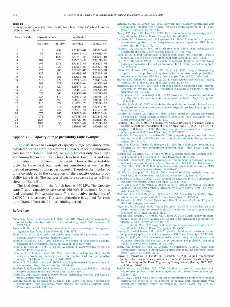
Table B1 shows an example of capacity outage probability tablecalculated for the froth hour of the UC schedule for the minimumcost solution (Tables 3 and A2). As Table 3 shows only three unitsare committed in the fourth hour, two base load units and oneintermediate unit. However in the construction of the probabilitytable the three peak load units are considered as well as themethod proposed in this paper suggests. Therefore the number ofunits considered in the calculation of the capacity outage prob-ability table is six. The number of possible capacity states is 24 asshown in Table B1.

The load demand in the fourth hour is 950 MW. The capacitystate 7, with capacity in service of 965 MW, is assigned for thisload demand. For capacity state 7 a cumulative probability of2.0792E�1 is selected. The same procedure is applied for eachhour (frame) from the 24-h scheduling period.

References

Ahmadi, A., Aghaei, J., Shayanfar, H.A., Rabiee, A., 2012. Mixed integer programmingof multiobjective hydro-thermal self scheduling. Appl. Soft Comput. 12,2137–2146.

Amjady, N., Shirzadi, A., 2009. Unit commitment using a new integer coded geneticalgorithm. Eur. Trans. Electr. Power 19, 1161–1176.

Billinton, R., Allan, R.N., 1988. Reliability Assessment of Large Electric PowerSystems. Kluwer Academic Publishers, Boston.

Billinton, R., Allan, R.N., 1992. Reliability Evaluation of Engineering Systems:Concepts and Techniques, second ed. Plenum Press, New York.

Billinton, R., Allan, R.N., 1996. Reliability Evaluation of Power Systems, second ed.Plenum Press, New York.

Billinton, R., Fotuhi-Firuzabad, M., 1994. Generating system operating healthanalysis considering stand-by units, interruptible load and postponableoutages. IEEE Trans. Power Syst. 9, 1618–1625.

Billinton, R., Fotuhi-Firuzabad, M., 2000. A reliability framework for generating unitcommitment. Electr. Power Syst. Res. 56, 81–88.

Bouffard, F., Galiana, F.D., 2004. An electricity market with a probabilistic spinningreserve criterion. IEEE Trans. Power Syst. 19, 300–307.

Čepin, M., 2011. Assessment of Power System Reliability: Methods and Applica-tions. Springer-Verlag, London.

Chandrasekaran, K., Hemamalini, S., Simon, S.P., Padhy, N.P., 2012. Thermal unitcommitment using binary/real coded artificial bee colony algorithm. Electr.Power Syst. Res. 84, 109–119.

Chandrasekaran, K., Simon, S.P., 2012. Network and reliability constrained unitcommitment problem using binary real coded firefly algorithm. Int. J. Electr.Power Energy Syst. 43, 921–932.

Cheng, C.P., Liu, C.W., Liu, C.C., 2002. Unit commitment by annealing-geneticalgorithm. Int. J. Electr. Power Energy Syst. 24, 149–158.

Damousis, I.G., Bakirtzis, A.G., Dokopoulos, P.S., 2004. A solution to the unit-commitment problem using integer-coded genetic algorithm. IEEE Trans.Power Syst. 19, 1165–1172.

Dasgupta, D., McGregor, D.R., 1994. Thermal unit commitment using geneticalgorithms. IEE Proc.-Gener. Transm. Distrib. 141, 459–465.

Datta, D., 2013. Unit commitment problem with ramp rate constraint using abinary-real-coded genetic algorithm. Appl. Soft Comput. 13, 3873–3883.

Dieu, V.N., Ongsakul, W., 2011. Augmented Lagrange Hopfield network basedLagrangian relaxation for unit commitment. Int. J. Electr. Power Energy Syst.33, 522–530.

Dillon, T.S., Edwin, K.W., Kochs, H.D., Taud, R.J., 1978. Integer Programmingapproach to the problem of optimal unit commitment with probabilisticreserve determination. IEEE Trans. Power Appar. Syst. PAS 97, 2154–2166.

Elsayed, S.M., Sarker, R.A., Essam, D.L., 2014. A new genetic algorithm for solvingoptimization problems. Eng. Appl. Artif. Intell. 27, 57–69.

Eshelman, L.J., Schaffer, J.D., 1993. Real-coded genetic algorithms and interval-schemata. In: Whitley, D. (Ed.), Foundation of Genetic Algorithms, 2. MorganKaufmann, pp. 187–202.

Georgopoulou, C.A., Giannakoglou, K.C., 2009. Two-level, two-objective evolution-ary algorithms for solving unit commitment problems. Appl. Energy 86,1229–1239.

Gjorgiev, B., Čepin, M., 2013. A multi-objective optimization based solution for thecombined economic-environmental power dispatch problem. Eng. Appl. Artif.Intell. 26, 417–429.

Gjorgiev, B., Kančev, D., Čepin, M., 2013. A new model for optimal generationscheduling of power system considering generation units availability. Int. J.Electr. Power Energy Syst. 47, 129–139.

Goldberg, D.E., Deb, K., 1991. A Comparative Analysis Of Selection Schemes Used InGenetic Algorithms. Foundation of Genetic Algorithms 1 (FOGA-1), pp. 69–93.

Guangbin, L., Billinton, R., 1994. Operating reserve risk assessment in compositepower systems. IEEE Trans. Power Syst. 9, 1270–1276.

Jalilzadeh, S., Shayeghi, H., Hadadian, H., 2009. Integrating generation and trans-mission networks reliability for unit commitment solution. Energy Convers.Manag. 50, 777–785.

Juste, K.A., Kita, H., Tanaka, E., Hasegawa, J., 1999. An evolutionary programmingsolution to the unit commitment problem. IEEE Trans. Power Syst. 14,1452–1459.

Kazarlis, S.A., Bakirtzis, A.G., Petridis, V., 1996. A genetic algorithm solution to theunit commitment problem. IEEE Trans. Power Syst. 11, 83–92.

Khan, M.E., Billinton, R., 1993. Generating unit commitment in composite genera-tion and transmission systems. Gener. Transm. Distrib. IEE Proc. C 140, 404–410.

Lee, T.-Y., Chen, C.-L., 2007. Unit commitment with probabilistic reserve: an IPSOapproach. Energy Convers. Manag. 48, 486–493.

Lei, W., Shahidehpour, M., Tao, L., 2008. Cost of reliability analysis based onstochastic unit commitment. IEEE Trans. Power Syst. 23, 1364–1374.

Li, D., Das, S., Pahwa, A., Deb, K., 2013. A multi-objective evolutionary approach forgenerator scheduling. Expert Syst. Appl. 40, 7647–7655.

Lu, Y., Zhou, J., Qin, H., Wang, Y., Zhang, Y., 2011. Chaotic differential evolutionmethods for dynamic economic dispatch with valve-point effects. Eng. Appl.Artif. Intell. 24, 378–387.

Mantawy, A.H., Abdel-Magid, Y.L., Selim, S.Z., 1998. A simulated annealing algo-rithm for unit commitment. IEEE Trans. Power Syst. 13, 197–204.

Michalewicz, Z., 1996. Genetic AlgorithmsþData Structures¼Evolution Programs,third ed. Springer, New York.

Neyestani, M., Farsangi, M.M., Nezamabadi-pour, H., 2010. A modified particleswarm optimization for economic dispatch with non-smooth cost functions.Eng. Appl. Artif. Intell. 23, 1121–1126.

Norouzi, M.R., Ahmadi, A., Nezhad, A.E., Ghaedi, A., 2014. Mixed integer program-ming of multi-objective security-constrained hydro/thermal unit commitment.Renew. Sustain. Energy Rev. 29, 911–923.

Orero, S.O., Irving, M.R., 1997. Large scale unit commitment using a hybrid geneticalgorithm. Int. J. Electr. Power Energy Syst. 19, 45–55.

Ouyang, Z., Shahidehpour, S.M., 1992. A hybrid artificial neural network-dynamicprogramming approach to unit commitment. IEEE Trans. Power Syst. 7, 236–242.

Özyön, S., Aydin, D., 2013. Incremental artificial bee colony with local search toeconomic dispatch problem with ramp rate limits and prohibited operatingzones. Energy Convers. Manag. 65, 397–407.

Saber, A.Y., Senjyu, T., Yona, A., Urasaki, N., Funabashi, T., 2007. Fuzzy unitcommitment solution—a novel twofold simulated annealing approach. Electr.Power Syst. Res. 77, 1699–1712.

Senjyu, T., Yamashiro, H., Uezato, K., Funabashi, T., 2002. A unit commitmentproblem by using genetic algorithm based on unit characteristic classification.in: Proceedings of the Power Engineering Society Winter Meeting, 2002, IEEE,vol. 51, pp. 58–63.

Senthil Kumar, V., Mohan, M.R., 2010. Solution to security constrained unitcommitment problem using genetic algorithm. Int. J. Electr. Power Energy Syst.32, 117–125.

Shi, L., Hao, J., Zhou, J., Xu, G., 2004. Ant colony optimization algorithmwith randomperturbation behavior to the problem of optimal unit commitment withprobabilistic spinning reserve determination. Electr. Power Syst. Res. 69,295–303.

Table B1Capacity outage probability table for the froth hour of the UC schedule for theminimum cost solution.

Capacity state Capacity service Probabilities

Out (MW) In (MW) Individual Cumulative

1 0 1237 7.2839E�01 1.0000Eþ002 55 1182 3.3953E�02 2.7161E�013 110 1127 5.2754E�04 2.3766E�014 162 1075 2.7907E�02 2.3713E�015 165 1072 2.7323E�06 2.0922E�016 217 1020 1.3008E�03 2.0922E�017 272 965 2.0212E�05 2.0792E�018 327 910 1.0468E�07 2.0790E�019 455 782 1.8005E�01 2.0790E�01

10 510 727 8.3928E�03 2.7849E�0211 565 672 1.3040E�04 1.9456E�0212 617 620 6.8984E�03 1.9326E�0213 620 617 6.7540E�07 1.2427E�0214 672 565 3.2156E�04 1.2427E�0215 727 510 4.9963E�06 1.2105E�0216 782 455 2.5877E�08 1.2100E�0217 910 327 1.1127E�02 1.2100E�0218 965 272 5.1865E�04 9.7324E�0419 1020 217 8.0587E�06 4.5459E�0420 1072 165 4.2631E�04 4.4653E�0421 1075 162 4.1738E�08 2.0224E�0522 1127 110 1.9872E�05 2.0182E�0523 1182 55 3.0876E�07 3.1036E�0724 1237 0 1.5991E�09 1.5991E�09


http://refhub.elsevier.com/S0952-1976(14)00234-6/sbref1













































































































Simon, S.P., Padhy, N.P., Anand, R.S., 2006. An ant colony system approach for unitcommitment problem. Int. J. Electr. Power Energy Syst. 28, 315–323.

Simopoulos, D.N., Kavatza, S.D., Vournas, C.D., 2006. Reliability constrained unitcommitment using simulated annealing. IEEE Trans. Power Syst. 21, 1699–1706.

Stoll, H.G., 1989. Least-Cost Electric Utility Planning. John Wiley & Sons, New York.Sun, L., Zhang, Y., Jiang, C., 2006. A matrix real-coded genetic algorithm to the unit

commitment problem. Electr. Power Syst. Res. 76, 716–728.Ting, T.O., Rao, M.V.C., Loo, C.K., 2006. A novel approach for unit commitment

problem via an effective hybrid particle swarm optimization. IEEE Trans. PowerSyst. 21, 411–418.

Todorovski, M., Rajicic, D., 2006. An initialization procedure in solving optimalpower flow by genetic algorithm. IEEE Trans. Power Syst. 21, 480–487.

Volkanovski, A., Mavko, B., Boševski, T., Čauševski, A., Čepin, M., 2008. Geneticalgorithm optimisation of the maintenance scheduling of generating units in apower system. Reliabil. Eng. Syst. Saf. 93, 779–789.

Walters, D.C., Sheble, G.B., 1993. Genetic algorithm solution of economic dispatchwith valve point loading. IEEE Trans. Power Syst. 8, 1325–1332.

Wong, K.P., Fung, C.C., 1993. Simulated annealing based economic dispatchalgorithm. IEE Proc.-Gener. Transm. Distrib. 140, 509–515.

Wood, A.J., Wollenberg, B.F., 1996. Power Generation, Operation, and Control,second ed. John Wiley & Sons, New York.

Yamashita, D., Niimura, T., Yokoyama, R., Marmiroli, M., 2010. Trade-off analysis ofCO2 versus cost by multi-objective unit commitment. In: Proceedings of thePower and Energy Society General Meeting, 2010 IEEE, pp. 1–6.

Yan-Fu, L., Pedroni, N., Zio, E., 2013. A Memetic evolutionary multi-objectiveoptimization method for environmental power unit commitment. IEEE Trans.Power Syst. 28, 2660–2669.




























multi-objective unit commitment with introduction of a methodology for probabilistic assessment of...

Documents