multi-objective optimization of mig welding and preheat

coatings

Article

Multi-Objective Optimization of MIG Welding and PreheatParameters for 6061-T6 Al Alloy T-Joints Using Artificial NeuralNetworks Based on FEM

Qing Shao 1, Fuxing Tan 1, Kai Li 1, Tatsuo Yoshino 2 and Guikai Guo 2,*

��

Citation: Shao, Q.; Tan, F.; Li, K.;

Yoshino, T.; Guo, G.k. Multi-Objective

Optimization of MIG Welding and

Preheat Parameters for 6061-T6 Al

Alloy T-Joints Using Artificial Neural

Networks Based on FEM. Coatings

2021, 11, 998. https://doi.org/

10.3390/coatings11080998

Academic Editor:

Tomasz Chmielewski

Received: 30 July 2021

Accepted: 18 August 2021

Published: 21 August 2021

Publisher’s Note: MDPI stays neutral

with regard to jurisdictional claims in

published maps and institutional affil-

iations.

Copyright: © 2021 by the authors.

Licensee MDPI, Basel, Switzerland.

This article is an open access article

distributed under the terms and

conditions of the Creative Commons

Attribution (CC BY) license (https://

creativecommons.org/licenses/by/

4.0/).

1 Maglev Technology Institute, CRRC Changchun Railway Vehicles Co., Ltd., Changchun 130062, China;[email protected] (Q.S.); [email protected] (F.T.); [email protected] (K.L.)

2 School of Mechanical and Aerospace Engineering, Jilin University, Changchun 130022, China;[email protected]

* Correspondence: [email protected]

Abstract: To control the welding residual stress and deformation of metal inert gas (MIG) welding,the influence of welding process parameters and preheat parameters (welding speed, heat input,preheat temperature, and preheat area) is discussed, and a prediction model is established to select theoptimal combination of process parameters. Thermomechanical numerical analysis was performed toobtain the residual welding deformation and stress according to a 100 × 150 × 50 × 4 mm aluminumalloy 6061-T6 T-joint. Owing to the complexity of the welding process, an optimal Latin hypercubesampling (OLHS) method was adopted for sampling with uniformity and stratification. Analysisof variance (ANOVA) was used to find the influence degree of welding speed (7.5–9 mm/s), heatinput (1500–1700 W), preheat temperature (80–125 ◦C), and preheat area (12–36 mm). The rangeof research parameters are according to the material, welding method, thickness of the weldingplate, and welding procedure specification. Artificial neural network (ANN) and multi-objectiveparticle swarm optimization (MOPSO) was combined to find the effective parameters to minimizewelding deformation and stress. The results showed that preheat temperature and welding speedhad the greatest effect on the minimization of welding residual deformation and stress, followed bythe preheat area, respectively. The Pareto front was obtained by using the MOPSO algorithm withε-dominance. The welding residual deformation and stress are the minimum at the same time, whenthe welding parameters are selected as preheating temperature 85 ◦C and preheating area 12 mm,welding speed is 8.8 mm/s and heat input is 1535 W, respectively. The optimization results werevalidated by the finite element (FE) method. The error between the FE results and the Pareto optimalcompromise solutions is less than 12.5%. The optimum solutions in the Pareto front can be chosen bydesigners according to actual demand.

Keywords: welding parameters; preheat parameters; welding deformation; welding stress; multi-objective optimization; artificial neural network; FEM simulation

1. Introduction

With the rapid development of rail vehicles in China in recent years, an increasingnumber of high requirements have been put forward for the materials used in railwayvehicles [1]. Among different lightweight materials, aluminum alloys possess an excellentstrength-to-weight ratio and are extensively used in subways, intercity trains, and high-speed electric multiple units (EMU) [2–4]. However, due to the high linear expansioncoefficient of 6061-T6, a study of methods to reduce the welding residual stress anddeformation is urgently needed [5,6].

Many scholars have chosen to study and optimize the welding process parameters toimprove the welding qualities and to reduce the welding residual deformation and residualtensile stress [7,8]. Kumar [9] studied the effects of MIG welding process parameters such

Coatings 2021, 11, 998. https://doi.org/10.3390/coatings11080998 https://www.mdpi.com/journal/coatings

https://www.mdpi.com/journal/coatings

https://www.mdpi.com

https://doi.org/10.3390/coatings11080998


https://creativecommons.org/

https://creativecommons.org/licenses/by/4.0/

https://creativecommons.org/licenses/by/4.0/


https://www.mdpi.com/journal/coatings

https://www.mdpi.com/article/10.3390/coatings11080998?type=check_update&version=1

Coatings 2021, 11, 998 2 of 20

as current, voltage, and preheat temperature and optimized them using gray-based Taguchimethodology. The influence of above parameters was determined by analysis of variance(ANOVA). Matthew [10] used a design of experiments (DOE) to study the welding processparameters, such as velocity, weld pressure, upset distance, and preheat temperature,on weld strength, heat affected zone, and energy usage for the friction welding of AISI1020 steel. Aalami-Aleagha [11] investigated the welding current of Al alloy T-joints in adouble-pulsed metal inert gas welding process. Finally, the optimization parameters ofthe best condition were gained by simulation. Khoshroyan [12] studied three modes ofcurrent, two different speeds, and two different sequences, through comparative analysis;the influence parameters of reducing transverse deformation were found.

Beyond the above processing parameters, the effect of preheating on welding parts issignificant. Preheating the parts to be welded above room temperature before welding isa method often used to improve the welding quality and the plastic deformation abilityof materials and to reduce welding stress to prevent cracks. Thus, many scholars havealso focused on this factor [13,14]. Asadi [15] studied temperature and residual stressfields in multipass TIG welds with different pipes, and found that preheating up to at least325 ◦C is essential to keep residual stress below the yield strength. Fallahi [16] employed3-D numerical models to study the behavior of residual stresses and entropy resultsfrom three common welding sequences at different preheating temperatures. Liang [17]simulated the MIG welding process of 6061-T6 thin plate for healthcare applicationsusing the commercial software ABAQUS to study the effect of different preheating weldingprocedures on residual stress in the aluminum alloy. Liu [18] used ANSYS and the Gaussianheat source model to study the distribution of the temperature field in the high-strengthsteel synchronizing process of preheating and welding. Considering boards of differentdimensions and different demands for the preheating width, some simulating evaluationswere done under the conditions of single preheat source and double preheat source toshow the feasibility of the preheat simulation method.

With an increasing number of variables listed in the research area and set as opti-mization parameters, it becomes increasingly difficult to find the optimal combination ofvariables. Many scholars have begun to study welding results prediction methods basedon artificial neural networks (ANN) and new optimization methods [19–23]. Bai [24] com-bined the inherent deformation method and the complex method to efficiently predict thewelding deformation of large and complex welded structures. Huang [25] used the localsolid model and global shell model to predict the deformation of laser welded thin platebased on inherent strain theory and considering geometrical imperfection in the numericalmodel. Zhang [26] proposed a new electron beam welding method to decrease the distor-tion of thin-walled structures. However, it is worthwhile to further study improvementin the accuracy of the surrogate model and to make the Pareto front of multi-objectiveoptimization solutions more uniform and diverse.

In this paper, the effects of the processing and preheat parameters of metal inert gas(MIG) welding in the modification of the residual deformation and stress distribution areboth investigated. The analysis of variance (ANOVA) was conducted by an optimal Latinhypercube sampling (OLHS) method to find the influence degree. The multi-objectiveparticle swarm optimization (MOPSO) based on ANN is innovatively adopted to optimizethe above parameters to gain the Pareto front.

2. Finite Element Simulation

A T-joint FE model is established for this study using Hypermesh. The dimensions ofthe web plate and flange plate are 200 mm, 80 mm, and 2 mm; 200 mm, 50 mm, and 2 mmrespectively, as shown in Figure 1. Many hexahedron elements and a few tetrahedronelements are adopted in the FE model to assure the quality of grids in the region of thewelding seams. To reduce the computation cost, the mesh size of elements in the region ofthe welding seam and the weld heat-affected zone were set as 1 mm, and the mesh size of

Coatings 2021, 11, 998 3 of 20

elements far away from the above region increased to 5 mm gradually. The numbers ofelements and nodes are 13,900 and 20,099, respectively.

Coatings 2021, 11, x FOR PEER REVIEW 3 of 21

of elements far away from the above region increased to 5 mm gradually. The numbers of elements and nodes are 13,900 and 20,099, respectively.

Figure 1. T-joint FE model.

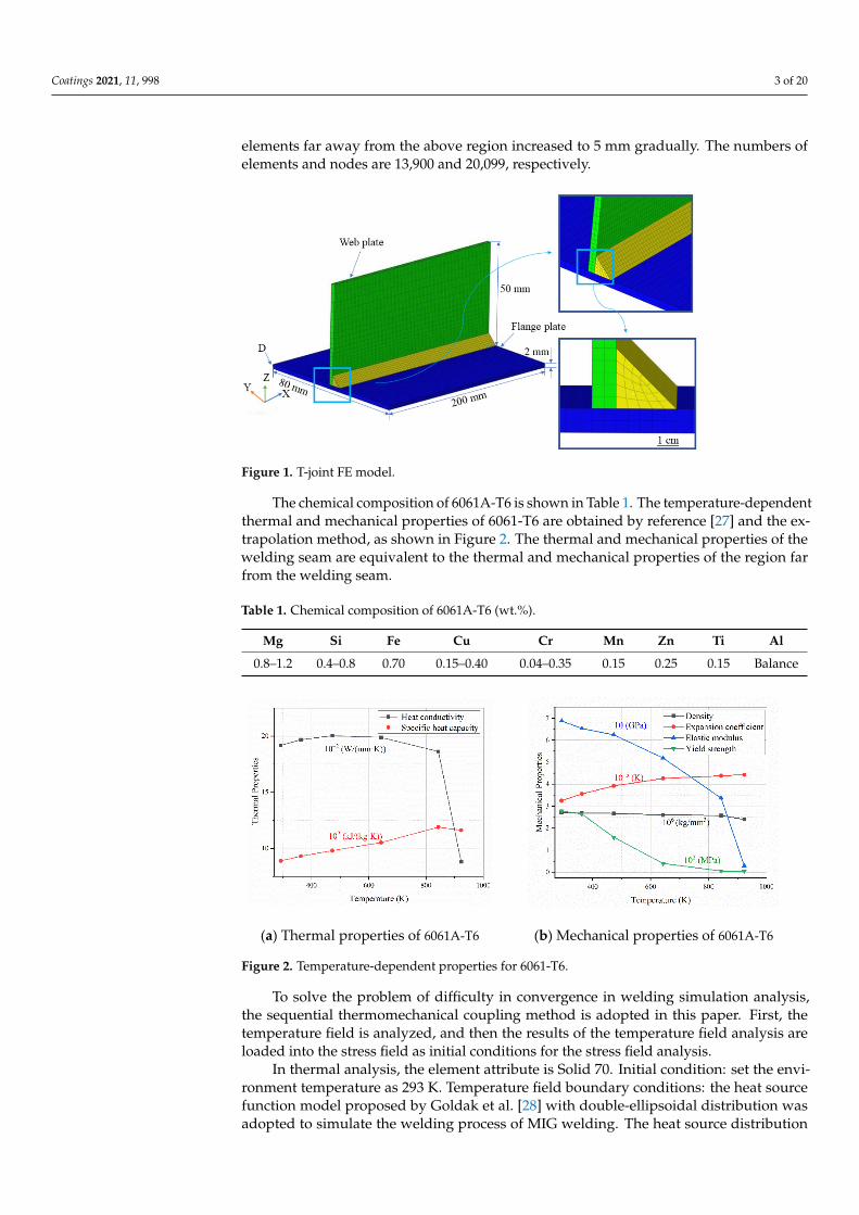
The chemical composition of 6061A-T6 is shown in Table 1. The temperature-depend-ent thermal and mechanical properties of 6061-T6 are obtained by reference [27] and the extrapolation method, as shown in Figure 2. The thermal and mechanical properties of the welding seam are equivalent to the thermal and mechanical properties of the region far from the welding seam.

(a) Thermal properties of 6061A-T6 (b) Mechanical properties of 6061A-T6

Figure 2. Temperature-dependent properties for 6061-T6.

Table 1. Chemical composition of 6061A-T6 (wt.%).

Mg Si Fe Cu Cr Mn Zn Ti Al 0.8–1.2 0.4–0.8 0.70 0.15–0.40 0.04–0.35 0.15 0.25 0.15 Balance

To solve the problem of difficulty in convergence in welding simulation analysis, the sequential thermomechanical coupling method is adopted in this paper. First, the temper-ature field is analyzed, and then the results of the temperature field analysis are loaded into the stress field as initial conditions for the stress field analysis.

In thermal analysis, the element attribute is Solid 70. Initial condition: set the envi-ronment temperature as 293 K. Temperature field boundary conditions: the heat source function model proposed by Goldak et al. [28] with double-ellipsoidal distribution was adopted to simulate the welding process of MIG welding. The heat source distribution of


The chemical composition of 6061A-T6 is shown in Table 1. The temperature-dependentthermal and mechanical properties of 6061-T6 are obtained by reference [27] and the ex-trapolation method, as shown in Figure 2. The thermal and mechanical properties of thewelding seam are equivalent to the thermal and mechanical properties of the region farfrom the welding seam.


Mg Si Fe Cu Cr Mn Zn Ti Al

0.8–1.2 0.4–0.8 0.70 0.15–0.40 0.04–0.35 0.15 0.25 0.15 Balance


of elements far away from the above region increased to 5 mm gradually. The numbers of elements and nodes are 13,900 and 20,099, respectively.


The chemical composition of 6061A-T6 is shown in Table 1. The temperature-depend-ent thermal and mechanical properties of 6061-T6 are obtained by reference [27] and the extrapolation method, as shown in Figure 2. The thermal and mechanical properties of the welding seam are equivalent to the thermal and mechanical properties of the region far from the welding seam.

(a) Thermal properties of 6061A-T6 (b) Mechanical properties of 6061A-T6



Mg Si Fe Cu Cr Mn Zn Ti Al 0.8–1.2 0.4–0.8 0.70 0.15–0.40 0.04–0.35 0.15 0.25 0.15 Balance

To solve the problem of difficulty in convergence in welding simulation analysis, the sequential thermomechanical coupling method is adopted in this paper. First, the temper-ature field is analyzed, and then the results of the temperature field analysis are loaded into the stress field as initial conditions for the stress field analysis.

In thermal analysis, the element attribute is Solid 70. Initial condition: set the envi-ronment temperature as 293 K. Temperature field boundary conditions: the heat source function model proposed by Goldak et al. [28] with double-ellipsoidal distribution was adopted to simulate the welding process of MIG welding. The heat source distribution of


To solve the problem of difficulty in convergence in welding simulation analysis,the sequential thermomechanical coupling method is adopted in this paper. First, thetemperature field is analyzed, and then the results of the temperature field analysis areloaded into the stress field as initial conditions for the stress field analysis.

In thermal analysis, the element attribute is Solid 70. Initial condition: set the envi-ronment temperature as 293 K. Temperature field boundary conditions: the heat sourcefunction model proposed by Goldak et al. [28] with double-ellipsoidal distribution wasadopted to simulate the welding process of MIG welding. The heat source distribution

Coatings 2021, 11, 998 4 of 20

of the two ellipsoids is shown in Equations (1) and (2), and the heat transfer coefficientis loaded on the free surface of the model. The application of the moving heat source isrealized by the moving welding heat source method [29]. The welding process of metalgradually filled is simulated by the birth-death method [30].

q f (x, y, z) =6√

3 f f Qa f bcπ

√π

exp

(−3

(x2

a2f+

y2

b2 +z2

c2

))(1)

qb(x, y, z) =6√

3 fbQabbcπ

√π

exp

(−3

(x2

a2b+

y2

b2 +z2

c2

))(2)

where af, ab, b, and c are the shape parameters of the heat input, respectively; Q is thethermal input power; ff is the energy distribution coefficient of the front half of the ellipsoid;and fb is the energy distribution coefficient of the back half of the ellipsoid. In general,ff = 0.4 and fb = 1.6, which are employed for the analysis optimization. According to theshape and size of the weld pool and the temperature field in the actual welding, the shapeparameters of the heat source are adjusted and the corresponding model parameters of thedouble ellipsoid heat source are af = 2 mm, ar = 3.5 mm, b = 2.2 mm, and c = 2 mm.

In mechanical analysis, the element attribute is Solid 185. Initial condition: the resultsof the temperature field analysis are set as initial conditions. Stress field constraint con-straints: all freedom of element D was constrained in Figure 1 to guarantee the convergenceof FE calculation.

3. Experiments and Finite Element Model Validation

Both the temperature fields and the stress fields were verified according to refer-ence [27] to verify the accuracy of the finite element model. In the experiment, the basematerial was 6061-T6 Al alloy. The arc welding robot system, produced by OTC in Japanis used for T-joint MIG welding. The filler wire adopted was ER5356 Al-Mg alloy witha diameter of 1.2 mm, and the feed rate of filler wire is 6 m/min. The welding processthroughout this work was shielded by pure argon at air flow rate of 25 L/min in theexperiment. The welding process parameters of both the experiment and the simulationare welding current 90 A, welding speed 60 cm/min, and welding angle 45◦.

According to reference [27], the layout of the measuring points of the web nearthe fusion zone is shown in Figure 3, each having a length of 5 mm, were installed atpoints A, B, and C. As shown in Figure 4, the time–temperature curves of experimentalmeasurements and simulation results are highly fitted. Curve A reaches the highesttemperature because point A is closest to the welding seam. In addition, the isothermcorresponding to the melting of the base metal is compared with the weld pool shapeobtained by the experiment with the same parameters, as shown in Figure 5, verifying theaccuracy of the result by simulation.


the two ellipsoids is shown in Equations (1) and (2), and the heat transfer coefficient is loaded on the free surface of the model. The application of the moving heat source is re-alized by the moving welding heat source method [29]. The welding process of metal gradually filled is simulated by the birth-death method [30].

2 2 2

2 2 2

6 3( , , ) exp 3f

fff

f Q x y zq x y za b ca bcπ π

= − + +

(1)

2 2 2

2 2 2

6 3( , , ) exp 3bb

bb

f Q x y zq x y za b ca bcπ π

= − + +

(2)

where af, ab, b, and c are the shape parameters of the heat input, respectively; Q is the thermal input power; ff is the energy distribution coefficient of the front half of the ellip-soid; and fb is the energy distribution coefficient of the back half of the ellipsoid. In general, ff = 0.4 and fb = 1.6, which are employed for the analysis optimization. According to the shape and size of the weld pool and the temperature field in the actual welding, the shape parameters of the heat source are adjusted and the corresponding model parameters of the double ellipsoid heat source are af = 2 mm, ar = 3.5 mm, b = 2.2 mm, and c = 2 mm.

In mechanical analysis, the element attribute is Solid 185. Initial condition: the results of the temperature field analysis are set as initial conditions. Stress field constraint con-straints: all freedom of element D was constrained in Figure 1 to guarantee the conver-gence of FE calculation.

3. Experiments and Finite Element Model Validation Both the temperature fields and the stress fields were verified according to reference

[27] to verify the accuracy of the finite element model. In the experiment, the base material was 6061-T6 Al alloy. The arc welding robot system, produced by OTC in Japan is used for T-joint MIG welding. The filler wire adopted was ER5356 Al-Mg alloy with a diameter of 1.2 mm, and the feed rate of filler wire is 6 m/min. The welding process throughout this work was shielded by pure argon at air flow rate of 25 L/min in the experiment. The weld-ing process parameters of both the experiment and the simulation are welding current 90 A, welding speed 60 cm/min, and welding angle 45°.

According to reference [27], the layout of the measuring points of the web near the fusion zone is shown in Figure 3, each having a length of 5 mm, were installed at points A, B, and C. As shown in Figure 4, the time–temperature curves of experimental measure-ments and simulation results are highly fitted. Curve A reaches the highest temperature because point A is closest to the welding seam. In addition, the isotherm corresponding to the melting of the base metal is compared with the weld pool shape obtained by the experiment with the same parameters, as shown in Figure 5, verifying the accuracy of the result by simulation.

Figure 3. Measuring points of temperature and stress field. Figure 3. Measuring points of temperature and stress field.

Coatings 2021, 11, 998 5 of 20Coatings 2021, 11, x FOR PEER REVIEW 5 of 21

Figure 4. Temperature–time curve comparison of simulated and experimental results.

Figure 5. Simulation and experiment comparison of bead width and depth.

The residual welding stress of the workpiece was measured by the blind hole method. Four strain gauges of 10 mm were located on the flange plate, from 1 to 4. Weld-ing residual stress and deformation comparison of the experimental measurements and simulation results of this paper and the simulation result of reference [27] are shown in Figure 6 and Table 2, respectively. As shown in Figure 6, the welding stress curves of the experimental measurements and simulation results are highly fitted. Furthermore, the de-viation of welding deformation between the simulation in this paper and experimental values is smaller than the deviation between the simulation in reference [27] and experi-ment values, which illustrates the effectiveness and high accuracy of the simulation method in this paper.





The residual welding stress of the workpiece was measured by the blind hole method. Four strain gauges of 10 mm were located on the flange plate, from 1 to 4. Weld-ing residual stress and deformation comparison of the experimental measurements and simulation results of this paper and the simulation result of reference [27] are shown in Figure 6 and Table 2, respectively. As shown in Figure 6, the welding stress curves of the experimental measurements and simulation results are highly fitted. Furthermore, the de-viation of welding deformation between the simulation in this paper and experimental values is smaller than the deviation between the simulation in reference [27] and experi-ment values, which illustrates the effectiveness and high accuracy of the simulation method in this paper.


The residual welding stress of the workpiece was measured by the blind hole method.Four strain gauges of 10 mm were located on the flange plate, from 1 to 4. Welding residualstress and deformation comparison of the experimental measurements and simulationresults of this paper and the simulation result of reference [27] are shown in Figure 6 andTable 2, respectively. As shown in Figure 6, the welding stress curves of the experimentalmeasurements and simulation results are highly fitted. Furthermore, the deviation ofwelding deformation between the simulation in this paper and experimental values issmaller than the deviation between the simulation in reference [27] and experiment values,which illustrates the effectiveness and high accuracy of the simulation method in this paper.

Table 2. Comparison of simulated and experimental results of welding deformation of T-joint.

Result Experiment [27] Simulation Deviation Simulation [27] Deviation

Distance along Z direction (mm) 1.1 1.08 1.8% 1.05 4.5%Angular deformation (◦) 1.61 1.54 4.3% 1.50 6.8%

Coatings 2021, 11, 998 6 of 20Coatings 2021, 11, x FOR PEER REVIEW 6 of 21

Figure 6. Comparison of simulated and experimental results of welding stress of a T-joint.

Table 2. Comparison of simulated and experimental results of welding deformation of T-joint.

Result Experiment [27] Simulation Deviation Simulation [27] Deviation Distance along Z direction (mm) 1.1 1.08 1.8% 1.05 4.5%

Angular deformation (°) 1.61 1.54 4.3% 1.50 6.8%

4. Multi-Objective Optimization Problem Among the different kinds of ANN, the back-propagation neural network (BPNN)

[31] was selected for its strong nonlinear relationship identification ability in finding the complex nonlinear relationship between welding process parameters and welding defor-mation in multiple groups of welding samples. This nonlinear relation is then used to predict the welding deformation and stress of the combination of several alternative weld-ing parameter samples and establishes the objective functions of the multi-objective opti-mization problem.

4.1. Selection of the Process Parameter Combination Based on OLHS Many process parameters affect the welding effect in MIG welding, such as welding

current, welding voltage, welding speed, and shielding gas flow rate. To reduce welding cracks, welding residual tensile stress, and ensure the depth of fusion, it is necessary to preheat thick welding parts before welding and to reasonably control the welding heat input. Therefore, the welding process parameters, preheat temperature, preheat area, welding speed, and welding heat input, which are effective in solving the above problem, are set as the research objects.

In the welding process of aluminum alloy, the welding heat input and preheat tem-perature must be strictly controlled to ensure the welding quality. If the preheat temper-ature is too low, the preheating effect before welding cannot be achieved. If the preheat temperature is too high, the performance of the aluminum alloy may be affected, leading to joint softening and the formation of a weld with a bad appearance. To prevent excessive local stress, the range of preheating must be no less than three times the thickness of the welded part on both sides of the weld and no more than 100 mm.

Figure 6. Comparison of simulated and experimental results of welding stress of a T-joint.

4. Multi-Objective Optimization Problem

Among the different kinds of ANN, the back-propagation neural network (BPNN) [31]was selected for its strong nonlinear relationship identification ability in finding the complexnonlinear relationship between welding process parameters and welding deformation inmultiple groups of welding samples. This nonlinear relation is then used to predict thewelding deformation and stress of the combination of several alternative welding parametersamples and establishes the objective functions of the multi-objective optimization problem.

4.1. Selection of the Process Parameter Combination Based on OLHS

Many process parameters affect the welding effect in MIG welding, such as weldingcurrent, welding voltage, welding speed, and shielding gas flow rate. To reduce weldingcracks, welding residual tensile stress, and ensure the depth of fusion, it is necessary topreheat thick welding parts before welding and to reasonably control the welding heatinput. Therefore, the welding process parameters, preheat temperature, preheat area,welding speed, and welding heat input, which are effective in solving the above problem,are set as the research objects.

In the welding process of aluminum alloy, the welding heat input and preheat temper-ature must be strictly controlled to ensure the welding quality. If the preheat temperatureis too low, the preheating effect before welding cannot be achieved. If the preheat tempera-ture is too high, the performance of the aluminum alloy may be affected, leading to jointsoftening and the formation of a weld with a bad appearance. To prevent excessive localstress, the range of preheating must be no less than three times the thickness of the weldedpart on both sides of the weld and no more than 100 mm.

Furthermore, if the welding heat input is too low and the welding speed is too fast,the welding arc will be unstable and will cause defects such as incomplete welding andslag clamping. However, when the welding heat input is too high and the welding speedis too slow, defects such as burn-through, bite edge, and coarse grain in the heat-affectedzone will easily occur, affecting the mechanical properties of the welding seam. Thus, asshown in Table 3, the range of research parameters is selected according to the material,welding method, thickness of the welding plate, and welding procedure specification.

Coatings 2021, 11, 998 7 of 20

Table 3. The range of research parameters.

Research Parameters Selected Range

Preheat temperature 80–125 ◦CPreheat area 12–36 mm

Welding speed 7.5–9 mm/sWelding heat input 1500–1700 W

Among many alternative combinations of welding process parameters, the set ofcombinations that can achieve the optimization goal is selected as the optimal plan. Thespare set is the solution space of this welding process parameter optimization system.Therefore, the greater the number of alternative welding process parameter combinations,the larger the optimization space and the greater the possibility of obtaining the optimalcombination. However, if all the combinations are listed, there are many redundant plans,which seriously affects the operational efficiency of the system.

Thus, OLHS [32] is utilized to generate samples within the design space. Preheattemperature, preheat area, welding speed, and welding input were chosen as the fourfactors, and for each factor, four levels were chosen. The total of all the process parametercombinations is 44, but the OLHS table only requires 72 combinations to completely reflectthe basic situation.

4.2. Design of a Back-Propagation Neural Network

A three-layer BPNN structure was chosen as the prediction model. The numbers ofneurons in the input layer and the output layer were four and one, respectively. Eachneuron of the input layer represents welding current, welding voltage, welding speed, andpreheat temperature. Welding deformation and welding stress were chosen as the outputlayer neuron to establish two four-input and one-output BPNN structure, respectively.

According to the formula, the number range of hidden layer neurons was calculated.Then, comparing the performance of BPNN under different hidden layer neurons, thenumber of neurons that could cause the performance of BPNN to reach the best predictionperformance was found.

hidden_num =√

m + n + a (3)

where hidden_num is the neuron number of the hidden layer, m and n are the neuronnumbers of the input layer and output layer, and a is an integer between 0 and 10. Thenumber of hidden layer neurons was set as an integer between 2 and 13 to train the network.According to the mean square error (MSE) value obtained in each training, it is found thatwhen the number of hidden layer nodes is 6, the MSE value trained by the network is thesmallest and the network performance is the best. Therefore, the network structure of thismodel is finally determined as 4-6-1, as shown in Figure 7.


Figure 7. Topology of the designed neural network.

4.3. Multi-Objective Particle Swarm Optimization Algorithm 4.3.1. Definition of Optimization

The prediction model of welding deformation and welding stress is equivalent to the objective function of the multi-objective optimization model. In this model, the optimiza-tion variable is the set of welding process parameters, and the objective variables are weld-ing deformation and welding stress. The functional relation between the optimization var-iable and the objective variable YWelding residual deformation, YWelding residual deformation = f(XPreheat temperature, XPreheat area, XWelding speed, XWelding heat input) is the nonlinear relation gained by the BPNN algorithm based on sample data. The constraint condition of optimization variable X is determined according to the welding equipment and product quality. The value range of each opti-mization variable in this paper is shown in Equation (4). The multi-objective optimization mathematical model of welding process parameter is established as follows:

( )Preheat temperature Preheat area Welding speed Welding heat input

Welding residual deformation Welding residual deformation

Preheat temperature

Preheat area

:

min : ( ) ( )

. . 80 C 125 C12 m

, ,

m

,

,

find

s t

X X X X

Y Y

XX

=

< <

< <

XX X

Welding speed

Welding heat input

36 mm45 cm/min 54 cm/min1500 W< 1700 W

XX

< <

<

(4)

where Welding residual deformation Welding residual deformation,( ) ( )Y YX X are the optimization objective func-tions, which are replaced by the prediction model in the actual optimization, YWelding residual

deformation and YWelding residual deformation represent the welding deformation and welding stress pre-dicted by the prediction model, respectively.

4.3.2. The Pareto Front It is difficult for each optimization objective to reach the optimal solution simultane-

ously, hence the Pareto optimal solution is usually discussed in the multi-objective opti-mization problem. In Pareto optimal solutions, a set of solutions is created such that none is dominant to the others.

5. Results and Discussion 5.1. Results of OLHS Table

According to the OLHS method and the selected range of the research parameters, 72 combinations of different values of each parameter are listed in Table 4. To study the influence of the welding heat input and prevent burn-through and excessive deformation,

Figure 7. Topology of the designed neural network.

Coatings 2021, 11, 998 8 of 20

4.3. Multi-Objective Particle Swarm Optimization Algorithm4.3.1. Definition of Optimization

The prediction model of welding deformation and welding stress is equivalent tothe objective function of the multi-objective optimization model. In this model, the opti-mization variable is the set of welding process parameters, and the objective variables arewelding deformation and welding stress. The functional relation between the optimizationvariable and the objective variable YWelding residual deformation, YWelding residual deformation =f (XPreheat temperature, XPreheat area, XWelding speed, XWelding heat input) is the nonlinear relationgained by the BPNN algorithm based on sample data. The constraint condition of opti-mization variable X is determined according to the welding equipment and product quality.The value range of each optimization variable in this paper is shown in Equation (4).The multi-objective optimization mathematical model of welding process parameter isestablished as follows:

f ind : X =(

XPreheat temperature, XPreheat area, XWelding speed, XWelding heat input

)min : YWelding residual deformation(X), YWelding residual deformation(X)s.t. 80 ◦C < XPreheat temperature < 125 ◦C

12 mm < XPreheat area < 36 mm45 cm/min < XWelding speed < 54 cm/min1500 W<XWelding heat input < 1700 W

(4)

where YWelding residual deformation(X), YWelding residual deformation(X) are the optimization ob-jective functions, which are replaced by the prediction model in the actual optimization,YWelding residual deformation and YWelding residual deformation represent the welding deformationand welding stress predicted by the prediction model, respectively.

4.3.2. The Pareto Front

It is difficult for each optimization objective to reach the optimal solution simulta-neously, hence the Pareto optimal solution is usually discussed in the multi-objectiveoptimization problem. In Pareto optimal solutions, a set of solutions is created such thatnone is dominant to the others.

5. Results and Discussion5.1. Results of OLHS Table

According to the OLHS method and the selected range of the research parameters,72 combinations of different values of each parameter are listed in Table 4. To study the in-fluence of the welding heat input and prevent burn-through and excessive deformation, thethickness of the aluminum sheet is increased to 4 mm, as shown in Figure 8. Furthermore,72 combinations are conducted using the temperature-dependent properties in Figure 2and the sequential thermomechanical coupling method mentioned in Section 2.

The optimization objectives of welding residual deformation and welding stress onlyreflect the results in the stress field after thermal-mechanical coupling analysis. Thus, theaverage central temperature of the heat source is extracted to reflect the rules of weldingheat input as a reference in the temperature field after thermal analysis. Finally, the averagecentral temperature of the heat source, the maximum deformation along the Z direction,and maximum welding tensile stress along path 1 are extracted as the result of eachcombination and are listed in Table 4.

Coatings 2021, 11, 998 9 of 20


the thickness of the aluminum sheet is increased to 4 mm, as shown in Figure 8. Further-more, 72 combinations are conducted using the temperature-dependent properties in Fig-ure 2 and the sequential thermomechanical coupling method mentioned in Section 2.

The optimization objectives of welding residual deformation and welding stress only reflect the results in the stress field after thermal-mechanical coupling analysis. Thus, the average central temperature of the heat source is extracted to reflect the rules of welding heat input as a reference in the temperature field after thermal analysis. Finally, the aver-age central temperature of the heat source, the maximum deformation along the Z direc-tion, and maximum welding tensile stress along path 1 are extracted as the result of each combination and are listed in Table 4.

Figure 8. Diagram of the T-joint used in OLHS plans.

Table 4. OLHS Plans and Results.

No

Optimization Variable Objective Variable

Preheat Temper-ature (X1) (°C)

Preheat Area (X2)

(mm)

Welding Speed (X3) (mm/s)

Welding Heat Input (X4) (W)

Heat Source Central Temper-

ature (°C)

Welding Residual Deformation (Y1)

(mm)

Welding Re-sidual Stress

(Y2) (MPa) 1 95 20 8.5 1570 1091 1.904 186.36 2 95 20 9 1700 1150 1.926 181.74 3 95 36 7.5 1700 1320 2.002 129.12 4 95 36 9 1630 1125 1.929 173.30 5 95 12 8 1700 1207 1.896 171.43 6 95 28 8.5 1700 1206 1.962 165.51 7 95 36 8 1500 1105 1.917 171.88 8 95 28 7.5 1570 1189 1.951 159.43 9 95 20 7.5 1500 1115 1.909 176.34

10 95 20 8 1630 1177 1.925 171.97 11 95 12 8.5 1630 1113 1.873 185.90 12 95 12 9 1570 1011 1.860 199.86 13 80 36 9 1700 1154 1.910 173.22 14 80 20 8.5 1500 1004 1.879 197.36 15 80 28 9 1500 974 1.880 198.75 16 80 20 8 1700 1216 1.910 167.56 17 80 36 7.5 1630 1227 1.920 148.05 18 80 12 7.5 1500 1074 1.851 184.19 19 80 28 8.5 1630 1137 1.905 179.16 20 80 20 7.5 1700 1265 1.932 155.23 21 80 28 7.5 1570 1169 1.916 166.15 22 80 12 8.5 1700 1158 1.867 181.54

Figure 8. Diagram of the T-joint used in OLHS plans.

Table 4. OLHS Plans and Results.

No


PreheatTemperature

(X1) (◦C)

PreheatArea (X2)

(mm)

WeldingSpeed (X3)

(mm/s)

WeldingHeat Input

(X4) (W)

Heat SourceCentral

Temperature (◦C)

Welding ResidualDeformation (Y1)

(mm)

WeldingResidual Stress

(Y2) (MPa)

1 95 20 8.5 1570 1091 1.904 186.362 95 20 9 1700 1150 1.926 181.743 95 36 7.5 1700 1320 2.002 129.124 95 36 9 1630 1125 1.929 173.305 95 12 8 1700 1207 1.896 171.436 95 28 8.5 1700 1206 1.962 165.517 95 36 8 1500 1105 1.917 171.888 95 28 7.5 1570 1189 1.951 159.439 95 20 7.5 1500 1115 1.909 176.3410 95 20 8 1630 1177 1.925 171.9711 95 12 8.5 1630 1113 1.873 185.9012 95 12 9 1570 1011 1.860 199.8613 80 36 9 1700 1154 1.910 173.2214 80 20 8.5 1500 1004 1.879 197.3615 80 28 9 1500 974 1.880 198.7516 80 20 8 1700 1216 1.910 167.5617 80 36 7.5 1630 1227 1.920 148.0518 80 12 7.5 1500 1074 1.851 184.1919 80 28 8.5 1630 1137 1.905 179.1620 80 20 7.5 1700 1265 1.932 155.2321 80 28 7.5 1570 1169 1.916 166.1522 80 12 8.5 1700 1158 1.867 181.5423 80 36 8 1500 1080 1.888 178.1624 80 28 8 1630 1175 1.918 169.4125 110 20 9 1500 1000 1.915 198.4226 110 36 9 1630 1148 1.964 166.2727 110 36 8.5 1700 1241 2.000 145.5328 110 12 9 1700 1137 1.900 185.6129 110 28 9 1570 1090 1.959 182.1730 110 20 8.5 1570 1109 1.932 183.0131 110 12 8 1630 1166 1.901 176.7532 110 36 7.5 1570 1225 1.984 137.6733 110 28 7.5 1630 1266 2.013 141.9834 110 20 7.5 1700 1305 2.001 144.4635 110 28 8 1500 1117 1.956 173.9136 110 12 8.5 1500 1009 1.870 198.5437 80 12 8 1570 1095 1.855 185.84

Coatings 2021, 11, 998 10 of 20

Table 4. Cont.

No


PreheatTemperature

(X1) (◦C)

PreheatArea (X2)

(mm)

WeldingSpeed (X3)

(mm/s)

WeldingHeat Input

(X4) (W)

Heat SourceCentral

Temperature (◦C)

Welding ResidualDeformation (Y1)

(mm)

WeldingResidual Stress

(Y2) (MPa)

38 80 28 7.5 1500 1113 1.901 174.4939 80 28 9 1700 1147 1.916 178.3040 80 36 8 1570 1140 1.901 169.8941 80 36 9 1500 983 1.876 192.9942 80 12 9 1630 1054 1.853 196.7843 80 12 8 1630 1146 1.864 180.6144 80 20 8 1500 1054 1.874 188.6845 80 12 7.5 1700 1243 1.892 162.0046 80 20 7.5 1630 1203 1.910 165.8447 80 20 9 1570 1023 1.873 197.4448 80 36 8.5 1570 1097 1.892 178.8449 125 12 9 1700 1149 1.919 183.7650 125 36 8 1630 1259 2.027 132.0351 125 28 8 1700 1305 2.066 137.4952 125 28 9 1500 1056 1.979 183.5153 125 20 8.5 1630 1170 1.979 173.8454 125 20 9 1630 1132 1.971 182.2655 125 20 7.5 1570 1203 1.982 160.3656 125 20 8.5 1700 1222 1.998 167.4157 125 20 8 1570 1164 1.971 171.7658 125 28 7.5 1630 1291 2.055 134.0759 125 36 7.5 1500 1188 1.998 138.3660 125 36 9 1570 1127 1.984 164.1461 125 12 7.5 1570 1168 1.918 172.1562 125 28 8.5 1500 1099 1.983 176.1963 125 28 9 1630 1156 2.011 171.1464 125 12 9 1500 976 1.884 202.6265 125 12 8 1500 1070 1.894 188.0266 125 36 8.5 1630 1209 2.013 144.8467 125 12 7.5 1630 1217 1.932 164.9068 125 28 8 1570 1189 2.013 156.8269 125 36 8 1700 1321 2.061 123.8770 125 12 8.5 1570 1089 1.898 189.9371 125 28 7.5 1700 1351 2.090 124.7972 125 20 7.5 1500 1185 1.963 170.15

5.2. Influence of Welding Parameters5.2.1. ANOVA for Heat Source Central Temperature, Welding Residual Deformation andWelding Residual Stress

To further study the influence of the process parameters, the influence degree ofeach parameter and the ANOVA for heat source central temperature, welding residualdeformation, and welding residual stress are discussed in this section according to theresults listed in Table 4.

The influence of different process parameters on the average central temperature ofthe heat source is shown in Figure 9. By and large, the preheat temperature, preheat area,and welding input are positively correlated with the heat source central temperature andwelding heat input, and the welding speed is a negative correlation with the target, asshown in Figure 9a–d. This indicates that the higher the total welding heat input per unittime and unit area, the higher the central temperature of the heat source will be.

Coatings 2021, 11, 998 11 of 20


5.2. Influence of Welding Parameters 5.2.1. ANOVA for Heat Source Central Temperature, Welding Residual Deformation and Welding Residual Stress

To further study the influence of the process parameters, the influence degree of each parameter and the ANOVA for heat source central temperature, welding residual defor-mation, and welding residual stress are discussed in this section according to the results listed in Table 4.

The influence of different process parameters on the average central temperature of the heat source is shown in Figure 9. By and large, the preheat temperature, preheat area, and welding input are positively correlated with the heat source central temperature and welding heat input, and the welding speed is a negative correlation with the target, as shown in Figure 9a–d. This indicates that the higher the total welding heat input per unit time and unit area, the higher the central temperature of the heat source will be.

(a) (b)

(c) (d)

Figure 9. The influence of different process parameters on the average central temperature of the heat source. (a) The influence of preheat temperature; (b) the influence of preheat area; (c) the influence of welding speed; (d) the influence of welding input.

The influence of different process parameters on welding residual deformation and stress is shown in Figure 10. Generally, the higher the heat input, the larger the residual deformation caused by temperature change. Because the deformation releases some

Figure 9. The influence of different process parameters on the average central temperature of the heat source. (a) Theinfluence of preheat temperature; (b) the influence of preheat area; (c) the influence of welding speed; (d) the influence ofwelding input.

The influence of different process parameters on welding residual deformation andstress is shown in Figure 10. Generally, the higher the heat input, the larger the residualdeformation caused by temperature change. Because the deformation releases some stress,the larger the deformation is, the smaller the residual stress. As shown in Figure 10a–d,the overall trend is the same as the above theory, but some points do not satisfy. Thatis probably because preheating raises the temperature around the weld seam, and anappropriate preheat temperature and preheat zone can reduce the temperature changegradient to reduce the welding tensile stress. Thus, it is necessary to further discussthe influence degree of each variable on the analysis target to find the influence of thisparameter on the temperature field and stress field and the best value of this parameter tocontrol the residual stress according to the actual demand in production.

Coatings 2021, 11, 998 12 of 20


stress, the larger the deformation is, the smaller the residual stress. As shown in Figure 10a–d, the overall trend is the same as the above theory, but some points do not satisfy. That is probably because preheating raises the temperature around the weld seam, and an appropriate preheat temperature and preheat zone can reduce the temperature change gradient to reduce the welding tensile stress. Thus, it is necessary to further discuss the influence degree of each variable on the analysis target to find the influence of this param-eter on the temperature field and stress field and the best value of this parameter to control the residual stress according to the actual demand in production.

(a) (b)

(c) (d)

Figure 10. The influence of different process parameters on welding residual deformation and stress. (a) Effect of preheat area and preheat temperature on welding residual deformation; (b) effect of preheat area and preheat temperature on welding residual stress; (c) effect of welding speed and welding input on welding residual deformation; (d) effect of weld-ing speed and welding input on welding residual stress.

To find the influence degree of each variable, the ANOVA is shown in Table 5 based on the OLHS plans and results. The F-value reflects the influence degree on the heat source central temperature, welding residual deformation, and welding residual stress, respectively. The greater the F-value is, the greater the correlation. The p-value reflects the significance level of the parameters. If the p-value is less than 0.0001, this parameter has a significant effect on the result. AB, AC, and so on in the first column reflect the effect of the interaction of the two parameters on the result.

Figure 10. The influence of different process parameters on welding residual deformation and stress. (a) Effect of preheatarea and preheat temperature on welding residual deformation; (b) effect of preheat area and preheat temperature onwelding residual stress; (c) effect of welding speed and welding input on welding residual deformation; (d) effect of weldingspeed and welding input on welding residual stress.

To find the influence degree of each variable, the ANOVA is shown in Table 5 basedon the OLHS plans and results. The F-value reflects the influence degree on the heatsource central temperature, welding residual deformation, and welding residual stress,respectively. The greater the F-value is, the greater the correlation. The p-value reflects thesignificance level of the parameters. If the p-value is less than 0.0001, this parameter has asignificant effect on the result. AB, AC, and so on in the first column reflect the effect of theinteraction of the two parameters on the result.

It can be seen from Table 5 that all the process parameters have a significant effecton the heat source central temperature, but the welding input has the greatest impact.However, for welding residual deformation, the preheat temperature and area have thegreatest impact. Furthermore, the welding speed and preheat area greatly affect the residualstress, and the preheat temperature has no significant effect on the residual stress.

Coatings 2021, 11, 998 13 of 20

Table 5. The ANOVA for heat source central temperature, welding residual deformation and stress.

SourceHeat source Central Temperature Welding Residual Deformation Welding Residual Stress

F-Value p-Value – F-Value p-Value – F-Value p-Value –

Preheat temperature(A) 883.33 <0.0001 significant 11,116.15 <0.0001 significant 239.05 0.0113 –

Preheat area (B) 515.71 <0.0001 significant 4272.88 <0.0001 significant 3955.25 <0.0001 significantWelding speed (C) 2400.74 <0.0001 significant 651.98 <0.0001 significant 4302.08 <0.0001 significantWelding input (D) 4125.25 <0.0001 significant 2105.38 <0.0001 significant 3097.19 <0.0001 significant

AB 16.61 0.0032 – 181.84 <0.0001 significant 166.65 0.0007 –AC 1.17 0.4567 – 7.1 0.022 – 7.9 0.059 –AD 0.4833 0.8381 – 23.23 0.0015 – 7.24 0.0676 –BC 1.43 0.3613 – 11.75 0.0072 – 21.29 0.0153 –BD 0.6517 0.7286 – 25.66 0.0012 – 11.12 0.0366 –CD 1.33 0.3961 – 27.01 0.001 – 20.04 0.0165 –

5.2.2. Discussion of Welding Residual Deformation and Stress

According to the conclusion of ANOVA, the preheat temperature has the greatestinfluence on the residual deformation of the T-joint, and the preheat area has a secondaryimpact on residual deformation. Thus, the temperature cycle curves of group 15 (pre-heat temperature 80 ◦C), group 52 (preheat temperature 125 ◦C), group 37 (preheat area12 mm), and group 40 (preheat area 36 mm) were extracted, and the corresponding residualdeformation results were discussed.

The temperature curve of the tracking points of different preheat temperatures andpreheat areas is shown in Figure 11. It can be seen from Figure 11a–d that the variationtrend of the temperature curve at tracking point A and tracking point B is consistent, whichshows that the temperature curve first remains unchanged, then rises rapidly, and finallyfalls rapidly to a stable level. The variation trend of the temperature curve at tracking pointC is to remain unchanged at first, then to rise slowly, and finally stabilize. In the 50 s, thetemperature curves of all tracking points coincide. In addition, the closer to the weld seam,the higher the maximum temperature and heat input at the tracking point, and the moredrastic the temperature change.

It can be seen that the variation trend of the temperature curve at each tracking point issimilar. The difference occurs between the maximum temperature at the tracking point andthe temperature at the end of the simulation. With the increase in the preheat temperatureand preheat area, the welding heat input and final temperature at the same tracking pointalso increase slightly. Preheating increased the depth of fusion and welding heat inputon the outer surface of the weld, reduced the temperature gradient and cooling rate afterwelding, improved the plastic deformation ability of the material, and reduced the weldingstress to prevent the formation of cracks. However, the residual deformation of groups52 (preheat temperature 125 ◦C) and 40 (preheat area 36 mm) are 5.27% and 2.48% higherthan the values for groups 15 (preheat temperature 80 ◦C) and 37 (preheat area 12 mm),respectively. Therefore, further optimization analysis is needed to obtain the minimumdeformation.

Figure 12 shows the distribution of equivalent residual stress and deformation ofT-joints after cooling. Because the transverse stress change is relatively small, this sectiononly considers the longitudinal stress.

According to the conclusion of ANOVA, the effects of welding speed and preheat zoneon the residual stress distribution of T-joints are discussed, respectively. The stress curvesof group 58 (welding speed 7.5 mm/s) and 63 (welding speed 9 mm/s) were extracted andthe corresponding residual stress results were discussed. As shown in Figure 12a, the fasterthe welding speed is, the lower welding heat input is, the higher the welding residualstress is, but the wider the distribution of welding residual compressive stress is.

Coatings 2021, 11, 998 14 of 20


mm), respectively. Therefore, further optimization analysis is needed to obtain the mini-mum deformation.

(a) (b)

(c) (d)

Figure 11. Temperature curves of tracking points at different preheat temperatures and areas. (a) Temperature curves of group 15; (b) temperature curves of group 52; (c) temperature curves of group 37; (d) temperature curves of group 40.

Figure 12 shows the distribution of equivalent residual stress and deformation of T-joints after cooling. Because the transverse stress change is relatively small, this section only considers the longitudinal stress.

According to the conclusion of ANOVA, the effects of welding speed and preheat zone on the residual stress distribution of T-joints are discussed, respectively. The stress curves of group 58 (welding speed 7.5 mm/s) and 63 (welding speed 9 mm/s) were ex-tracted and the corresponding residual stress results were discussed. As shown in Figure 12a, the faster the welding speed is, the lower welding heat input is, the higher the weld-ing residual stress is, but the wider the distribution of welding residual compressive stress is.

As shown in Figure 12b, the stress curves of groups 37 (preheat area 12 mm) and 40 (preheat area 36 mm) were extracted and the corresponding residual stress results were discussed. The wider the preheat zone, the higher welding heat input is, the lower the welding residual stress, but the wider the residual tensile stress distribution. The simula-tion results showed that preheating can reduce the longitudinal residual stress near the

Figure 11. Temperature curves of tracking points at different preheat temperatures and areas. (a) Temperature curves ofgroup 15; (b) temperature curves of group 52; (c) temperature curves of group 37; (d) temperature curves of group 40.

As shown in Figure 12b, the stress curves of groups 37 (preheat area 12 mm) and 40(preheat area 36 mm) were extracted and the corresponding residual stress results werediscussed. The wider the preheat zone, the higher welding heat input is, the lower thewelding residual stress, but the wider the residual tensile stress distribution. The simulationresults showed that preheating can reduce the longitudinal residual stress near the weldingbeam. However, the wider preheat area can increase the area of tensile stress, which is notgood for the fatigue strength of parts.

In practice, preheating of the base material is often used to improve the weldingprocess and improve the welding quality. The preheat temperature should not be toohigh or too low. Too high a temperature will affect the welding efficiency, and too lowa temperature will produce limited improvement of welding deformation and weldingstress, so it is necessary to choose the appropriate preheat temperature.

Coatings 2021, 11, 998 15 of 20


welding beam. However, the wider preheat area can increase the area of tensile stress, which is not good for the fatigue strength of parts.

In practice, preheating of the base material is often used to improve the welding pro-cess and improve the welding quality. The preheat temperature should not be too high or too low. Too high a temperature will affect the welding efficiency, and too low a temper-ature will produce limited improvement of welding deformation and welding stress, so it is necessary to choose the appropriate preheat temperature.

(a) (b)

Figure 12. Residual stress curve along path 1 at different welding speeds and areas. (a) Residual stress curves of groups 58 and 63; (b) residual stress curves of groups 37 and 40.

5.3. Performance of BPNN For further optimization analysis, the BPNN prediction model is established to reflect

optimization objectives in this section. To test the BPNN model, the data in Table 4 are separated into 70% training part, 15% validation part, and 15% testing part.

Additionally, the sigmoid function is selected as the transfer function of neurons in the hidden layer and the output layer of the network. MSE is selected as the evaluation index of network performance. The calculation formula of MSE is:

2

1

1 (y )q

i ii

MSE oq =

= − (5)

where q , yi, and oi represent the number of output neurons, the expected value and pre-dicted value of the ith output neuron, respectively. Figure 13 shows the network error curve, and the least MSE = 0.0019538 illustrates that the BPNN model gains the best vali-dation performance at epoch 12.

Figure 13. Network error curve obtained from the performance test with the least MSE.

Figure 12. Residual stress curve along path 1 at different welding speeds and areas. (a) Residual stress curves of groups 58and 63; (b) residual stress curves of groups 37 and 40.

5.3. Performance of BPNN

For further optimization analysis, the BPNN prediction model is established to reflectoptimization objectives in this section. To test the BPNN model, the data in Table 4 areseparated into 70% training part, 15% validation part, and 15% testing part.

Additionally, the sigmoid function is selected as the transfer function of neurons inthe hidden layer and the output layer of the network. MSE is selected as the evaluationindex of network performance. The calculation formula of MSE is:

MSE =1q

q

∑i=1

(yi − oi)

2

(5)

where q, yi, and oi represent the number of output neurons, the expected value andpredicted value of the ith output neuron, respectively. Figure 13 shows the network errorcurve, and the least MSE = 0.0019538 illustrates that the BPNN model gains the bestvalidation performance at epoch 12.


welding beam. However, the wider preheat area can increase the area of tensile stress, which is not good for the fatigue strength of parts.

In practice, preheating of the base material is often used to improve the welding pro-cess and improve the welding quality. The preheat temperature should not be too high or too low. Too high a temperature will affect the welding efficiency, and too low a temper-ature will produce limited improvement of welding deformation and welding stress, so it is necessary to choose the appropriate preheat temperature.

(a) (b)

Figure 12. Residual stress curve along path 1 at different welding speeds and areas. (a) Residual stress curves of groups 58 and 63; (b) residual stress curves of groups 37 and 40.

5.3. Performance of BPNN For further optimization analysis, the BPNN prediction model is established to reflect

optimization objectives in this section. To test the BPNN model, the data in Table 4 are separated into 70% training part, 15% validation part, and 15% testing part.

Additionally, the sigmoid function is selected as the transfer function of neurons in the hidden layer and the output layer of the network. MSE is selected as the evaluation index of network performance. The calculation formula of MSE is:

2

1

1 (y )q

i ii

MSE oq =

= − (5)

where q , yi, and oi represent the number of output neurons, the expected value and pre-dicted value of the ith output neuron, respectively. Figure 13 shows the network error curve, and the least MSE = 0.0019538 illustrates that the BPNN model gains the best vali-dation performance at epoch 12.

Figure 13. Network error curve obtained from the performance test with the least MSE. Figure 13. Network error curve obtained from the performance test with the least MSE.

The precision distribution of the training and test samples are shown in Figure 13. Theaggregation point along the 45◦ line indicates that the predicted value is close to the truevalues. The accuracies of the models can be verified by multiple correlation coefficients R.The equation for R is expressed as

Coatings 2021, 11, 998 16 of 20

R =

q∑

i=1(yi − y)(oi − y)√

q∑

i=1(yi − y)

2 q∑

i=1(oi − y)

2(6)

where yi is the expected value of the ith output neuron; oi is the predictive value; y is theaverage of expected values; and q is the number of plans. An R value close to 1 indicates ahigh degree of coincidence between the origin and the fitting line of the predicted data anda good fitting effect.

As can be observed in Figure 14a, the data points of the training sample were com-pletely coincident with the fitting line (R = 0.999) indicating that the prediction model madefull use of the data in the training sample. In Figure 14b,c, the degree of coincidence of datapoints and fitting lines of the verification samples and the test samples was high, and the Rvalue was 0.990 and 0.995, respectively, indicating that the prediction model had a goodprediction effect. Moreover, the difference in R values between the verification samplesand the test samples is not large, indicating that the prediction model is relatively robust.


The precision distribution of the training and test samples are shown in Figure 13. The aggregation point along the 45° line indicates that the predicted value is close to the true values. The accuracies of the models can be verified by multiple correlation coeffi-cients R. The equation for R is expressed as

12 2

1 1

( )( )

( ) ( )

q

i ii

q q

i ii i

y y o yR

y y o y

=

= =

− −=

− −

(6)

where yi is the expected value of the ith output neuron; oi is the predictive value; y is the average of expected values; and q is the number of plans. An R value close to 1 indicates a high degree of coincidence between the origin and the fitting line of the predicted data and a good fitting effect.

As can be observed in Figure 14a, the data points of the training sample were com-pletely coincident with the fitting line (R = 0.999) indicating that the prediction model made full use of the data in the training sample. In Figure 14b,c, the degree of coincidence of data points and fitting lines of the verification samples and the test samples was high, and the R value was 0.990 and 0.995, respectively, indicating that the prediction model had a good prediction effect. Moreover, the difference in R values between the verification samples and the test samples is not large, indicating that the prediction model is relatively robust.

(a) (b)


(c) (d)

Figure 14. Performance of BPNN. (a) Fitting situation of the training group; (b) fitting situation of the validation group; (c) fitting situation of the test group; (d) fitting situation of all groups.

5.4. Optimal Values of Design Parameters for Minimizing Objective Functions According to the discussion results in Section 5.2, the variation trend of welding re-

sidual stress is opposite that of residual deformation. To obtain the solution that meets both the design requirements according to the facts, multi-objective optimization is needed. Based on the BPNN prediction model, the MOPSO algorithm withε -dominance proposed by Mostaghim et al. [33] is used to optimize the mathematical problem in Sec-tion 4.3.1. The MOPSO algorithm [34] was selected to obtain the Pareto front of the objec-tives for its effective searchability. In addition, the ε -dominance method can find solu-tions much faster and gain better convergence and diversity. The MOPSO algorithm withε -dominance only considers the velocity and position variation of the particles when searching the Pareto front, which is more fitted in manufacturing problems. The flowchart of the multi-objective optimization method based on the MOPSO algorithm withε -dom-inance is shown in Figure 15.

Figure 15. Flowchart of the multi-objective optimization method based on MOPSO algorithm withε -dominance.

Figure 14. Performance of BPNN. (a) Fitting situation of the training group; (b) fitting situation ofthe validation group; (c) fitting situation of the test group; (d) fitting situation of all groups.

Coatings 2021, 11, 998 17 of 20

5.4. Optimal Values of Design Parameters for Minimizing Objective Functions

According to the discussion results in Section 5.2, the variation trend of weldingresidual stress is opposite that of residual deformation. To obtain the solution that meetsboth the design requirements according to the facts, multi-objective optimization is needed.Based on the BPNN prediction model, the MOPSO algorithm with ε-dominance proposedby Mostaghim et al. [33] is used to optimize the mathematical problem in Section 4.3.1.The MOPSO algorithm [34] was selected to obtain the Pareto front of the objectives forits effective searchability. In addition, the ε-dominance method can find solutions muchfaster and gain better convergence and diversity. The MOPSO algorithm with ε-dominanceonly considers the velocity and position variation of the particles when searching thePareto front, which is more fitted in manufacturing problems. The flowchart of the multi-objective optimization method based on the MOPSO algorithm with ε-dominance is shownin Figure 15.


(c) (d)

Figure 14. Performance of BPNN. (a) Fitting situation of the training group; (b) fitting situation of the validation group; (c) fitting situation of the test group; (d) fitting situation of all groups.

5.4. Optimal Values of Design Parameters for Minimizing Objective Functions According to the discussion results in Section 5.2, the variation trend of welding re-

sidual stress is opposite that of residual deformation. To obtain the solution that meets both the design requirements according to the facts, multi-objective optimization is needed. Based on the BPNN prediction model, the MOPSO algorithm withε -dominance proposed by Mostaghim et al. [33] is used to optimize the mathematical problem in Sec-tion 4.3.1. The MOPSO algorithm [34] was selected to obtain the Pareto front of the objec-tives for its effective searchability. In addition, the ε -dominance method can find solu-tions much faster and gain better convergence and diversity. The MOPSO algorithm withε -dominance only considers the velocity and position variation of the particles when searching the Pareto front, which is more fitted in manufacturing problems. The flowchart of the multi-objective optimization method based on the MOPSO algorithm withε -dom-inance is shown in Figure 15.

Figure 15. Flowchart of the multi-objective optimization method based on MOPSO algorithm withε -dominance.

Figure 15. Flowchart of the multi-objective optimization method based on MOPSO algorithm with ε-dominance.

The initial parameters for the MOPSO algorithm with ε-dominance are as follows: thenumbers of population and repository size are both 100; the inertial weight ω is 0.73; theaccelerated constants c1 and c2 are both 1.5; and the maximum number of iterations Maxy-gen is 1000. All parameters and results in the optimization domain are normalized to the0–1 region before optimization. After 950 iterations, the Pareto fronts of the two-objectivemodel are shown in Figure 15. The calculation time in MATLAB was approximately 18.5 s.The 1st objective presents the welding residual deformation, and the 2nd objective presentsthe welding residual stress. In Figure 16, the star symbol presents the Pareto front to reflectthe optimal solutions for different objectives. The Pareto optimal sets are evenly distributedalong the Pareto frontier, which indicates that the MOPSO algorithm with ε-dominancehas more uniform distribution characteristics.

Coatings 2021, 11, 998 18 of 20


The initial parameters for the MOPSO algorithm withε -dominance are as follows: the numbers of population and repository size are both 100; the inertial weight ω is 0.73; the accelerated constants c1 and c2 are both 1.5; and the maximum number of iterations Maxygen is 1000. All parameters and results in the optimization domain are normalized to the 0–1 region before optimization. After 950 iterations, the Pareto fronts of the two-objective model are shown in Figure 15. The calculation time in MATLAB was approxi-mately 18.5 s. The 1st objective presents the welding residual deformation, and the 2nd objective presents the welding residual stress. In Figure 16, the star symbol presents the Pareto front to reflect the optimal solutions for different objectives. The Pareto optimal sets are evenly distributed along the Pareto frontier, which indicates that the MOPSO al-gorithm withε -dominance has more uniform distribution characteristics.

Figure 16. The Pareto optimal front by the MOPSO algorithm with ε -dominance.

5.5. Simulation Experiments Confirmation Three representative optimal solutions were selected from the Pareto front. Case 1

had the minimum value of the 1st objective. Case 2 had the minimum value of the 2nd objective. Case 3 was the compromise solution of the 1st objectives and the 2nd objective. The representative optimal solutions of different objectives are listed in Table 6. The re-sults indicated that the optimization was consistent with the FE results. The error between the FE results and three representative optimal solutions selected from the Pareto front was less than 12.5%. These compromise solutions help the designers to select appropriate factors for the MIG welding process according to the actual requirements and reduce the dependence on work experience.

Table 6. Optimal compromise solution of two-objective optimization models.

No. Result Type Preheat Tem-perature (°C)

Preheat Area (mm)

Welding Speed (mm/s)

Welding Heat Input (W)

Welding Resid-ual Defor-

mation

Welding Resid-ual Stress

Case 1 Optimization

119 33 7.5 1692 0.985 0.616

FE 0.862 0.665

Case 2 Optimization

81 36 7.6 1653 0.886 1.000

FE 0.935 0.928

Case 3 Optimization

85 12 8.8 1535 0.927 0.721

FE 0.881 0.786

6. Conclusion A validated FE model of 6061-T6 Al alloy T-joint is used to study the influence of

welding process parameters and preheat parameters on welding residual deformation

Figure 16. The Pareto optimal front by the MOPSO algorithm with ε-dominance.

5.5. Simulation Experiments Confirmation

Three representative optimal solutions were selected from the Pareto front. Case 1had the minimum value of the 1st objective. Case 2 had the minimum value of the 2ndobjective. Case 3 was the compromise solution of the 1st objectives and the 2nd objective.The representative optimal solutions of different objectives are listed in Table 6. The resultsindicated that the optimization was consistent with the FE results. The error between theFE results and three representative optimal solutions selected from the Pareto front was lessthan 12.5%. These compromise solutions help the designers to select appropriate factors forthe MIG welding process according to the actual requirements and reduce the dependenceon work experience.

Table 6. Optimal compromise solution of two-objective optimization models.

No. Result TypePreheat

Temperature(◦C)

Preheat Area(mm)

WeldingSpeed(mm/s)

Welding HeatInput (W)

WeldingResidual

Deformation

WeldingResidual

Stress

Case 1Optimization

119 33 7.5 16920.985 0.616

FE 0.862 0.665

Case 2Optimization

81 36 7.6 16530.886 1.000

FE 0.935 0.928

Case 3Optimization

85 12 8.8 15350.927 0.721

FE 0.881 0.786

6. Conclusions

A validated FE model of 6061-T6 Al alloy T-joint is used to study the influence ofwelding process parameters and preheat parameters on welding residual deformation andstress. The multi-objective optimization method based on a neural network is adopted tooptimize the above parameters to gain the Pareto front. The conclusions of this paper areas follows:

(1) The thermal elastoplastic method was used to simulate the residual deformationand stress of 6061-T6 aluminum alloy T-joint in ANSYS. The simulation results arebasically consistent with the measured data, and the error is within 5%.

(2) The OLHS and ANOVA method were adopted to sample with uniformity and findthe influence degree. The results showed that preheat temperature and welding speed

Coatings 2021, 11, 998 19 of 20

had the greatest effect on the minimization of welding residual deformation andstress, respectively, followed by the preheat area.

(3) Preheating can reduce the temperature gradient and cooling rate after welding andreduced the welding stress to prevent the formation of cracks. However, the higherthe preheat temperature is, the larger the residual deformation is. Furthermore, thesimulation results showed that preheating can reduce the longitudinal residual stressnear the welding beam. However, the wider preheat area can increase the area oftensile stress, which is not good for the fatigue strength of parts. In addition, thefaster the welding speed is, the higher the welding residual stress is, but the widerthe distribution of welding residual compressive stress is.

(4) Artificial neural network-based MOPSO was used to optimize the effective parametersto minimize welding deformation and stress. The BPNN was selected to predict thevalue of the objective functions. The R values were 0.990 and 0.995, respectively,indicating that the prediction model had a good prediction effect.

(5) Welding residual deformation and stress are at the minimum at the same time, whenthe welding parameters are selected as preheating temperature 85 ◦C and preheatingarea 12 mm, welding speed 8.8 mm/s and heat input 1535 W, respectively. The Paretofront was obtained by using the MOPSO algorithm with ε-dominance. The errorbetween the FE results and the Pareto optimal compromise solutions is less than12.5%. The designers can select one solution from many Pareto solutions according topractical needs.

(6) Further, in order to further verify the reliability of the prediction, we will test andverify the welding results in the test group in the future, and obtain more useful con-clusions by comparing the change rules of welding heat curve, residual deformationand stress.

Author Contributions: Q.S. developed the conceptualization, methodology, investigation, formalanalysis and wrote original draft; F.T. and K.L. developed the idea of the study, and helped to draftthe manuscript; T.Y. and G.-k.G. contributed to the acquisition and interpretation of data; G.-k.G.provided critical review and substantially revised the manuscript. All authors have read and agreedto the published version of the manuscript.

Funding: This work was supported by the Consultant and Research Project of the Chinese Academyof Engineering (Grant No. 2019-JL-7), the National Science Foundation of China (Grant No. 11502092),and the Plan for Scientific and Technological Development of Jilin Province (Grant No. 20200201272JC).

Institutional Review Board Statement: Not applicable.

Informed Consent Statement: Not applicable.

Data Availability Statement: The raw/processed data required to reproduce these findings will bemade available on email request.

Conflicts of Interest: The authors declare no conflict of interest.

References1. Zhang, W.; Miao, B. Development trend and prospect of key technologies for next generation high speed trains. Electri. Drive

Locomot. 2018, 1, 1–12.2. Yang, S.; Zhang, D.; Tuo, W.; Yu, Z. Microstructures and properties of extruded Al-0.6Mg-0.6Si aluminium alloy for high-speed

vehicle. Procedia Eng. 2014, 81, 598–603. [CrossRef]3. Çam, G.; Ipekoglu, G. Recent developments in joining of aluminum alloys. Int. J. Adv. Manuf. Technol. 2017, 91, 1851–1866.

[CrossRef]4. Rozumek, D.; Lewandowski, J.; Lesiuk, G.; Correia, J. The influence of heat treatment on the behavior of fatigue crack growth in

welded joints made of S355 under bending loading. Int. J. Fatigue 2020, 131, 105328. [CrossRef]5. Yi, J.; Zhang, J.; Cao, S.; Guo, P. Effect of welding sequence on residual stress and deformation of 6061-T6 aluminium alloy

automobile component. Trans. Nonferrous Met. Soc. Chin. 2019, 29, 287–295. [CrossRef]6. Shao, Q.; Xu, T.; Yoshino, T.; Song, N. Multi-objective optimization of gas metal arc welding parameters and sequences for

low-carbon steel (Q345D) T joints. J. Iron Steel Res. 2017, 24, 544–555. [CrossRef]

http://doi.org/10.1016/j.proeng.2014.10.046

http://doi.org/10.1007/s00170-016-9861-0

http://doi.org/10.1016/j.ijfatigue.2019.105328

http://doi.org/10.1016/S1003-6326(19)64938-1

http://doi.org/10.1016/S1006-706X(17)30082-1

Coatings 2021, 11, 998 20 of 20

7. Maneiah, D.; Debashis, M.; Prahlada, R.K.; Brahma, R.K. Process parameters optimization of friction stir welding for optimumtensile strength in Al 6061-T6 alloy butt welded joints. Mate. Today 2020, 27, 904–908. [CrossRef]

8. Yang, X.; Chen, H.; Zhu, Z.; Cai, C.; Zhang, C. Effect of shielding gas flow on welding process of laser-arc hybrid welding andMIG welding. J. Manuf. Process. 2019, 38, 530–542. [CrossRef]

9. Kumar, S.; Singh, R. Optimization of process parameters of metal inert gas welding with preheating on AISI 1018 mild steel usinggrey based Taguchi method. Measurement 2019, 148, 106924. [CrossRef]

10. Matthew, R.K.; Steven, R.S.; Daniel, C.A.; Jeffrey, F.; Ryan, H. Experimental investigation of linear friction welding of AISI 1020steel with pre-heating. J. Manuf. Processes 2019, 39, 26–39.

11. Aalami-Aleagha, M.E.; Foroutan, M.; Feli, S.; Nikabadi, S. Analysis preheat effect on thermal cycle and residual stress in a weldedconnection by FE simulation. Int. J. Pres. Ves. Pip. 2014, 114, 69–75. [CrossRef]

12. Khoshroyan, A.; Darvazi, A.R. Effects of welding parameters and welding sequence on residual stress and distortion in Al6061-T6aluminum alloy for T-shaped welded joint. Trans. Nonferrous Met. Soc. Chin. 2020, 30, 76–89. [CrossRef]

13. Ashu, G.; Madhav, R.; Anirban, B. Metallurgical behavior and variation of vibro-acoustic signal during preheating assistedfriction stir welding between AA6061-T6 and AA7075-T651 alloys. Trans. Nonferrous Met. Soc. Chin. 2019, 29, 1610–1620.

14. Zhu, C.; Tang, X.; He, Y.; Lu, F.; Cui, H. Effect of preheating on the defects and microstructure in NG-GMA welding of 5083Al-alloy. J. Mate. Process. Technol. 2018, 251, 214–224. [CrossRef]

15. Asadi, P.; Alimohammadi, S.; Kohantorabi, O.; Fazli, A.; Akbari, M. Effects of material type, preheating and weld pass number onresidual stress of welded steel pipes by multi-pass TIG welding. Therm. Sci. Eng. Prog. 2020, 16, 100462. [CrossRef]

16. Fallahi, A.; Jafarpur, A.; Nami, M.R. Analysis of welding conditions based on induced thermal irreversibilities in weldedstructures: Cases of welding sequences and preheating treatment. Sci. Iran 2011, 18, 398–406. [CrossRef]

17. Liang, Y.; Wang, M.; Wang, J.; Chen, X.; P, G.E. Effect of pre-heating on residual stress in aluminum alloy joint for healthcareapplications. Electr. Weld. Mach. 2015, 45, 54–58.

18. Liu, B. The Research of Synchronizing Process of Preheating and Welding for High Strength Steel. Master’s Thesis, Hehaiuniversity, Jiangsu, China, June 2016.

19. Wu, C.; Kim, J.W. Numerical prediction of deformation in thin-plate welded joints using equivalent thermal strain method. ThinWalled Struct. 2020, 157, 107033. [CrossRef]

20. Chang, Y.; Yue, J.; Guo, R.; Liu, W.; Li, L. Penetration quality prediction of asymmetrical fillet root welding based on optimizedBP neural network. J. Manuf. Process. 2020, 50, 247–254. [CrossRef]

21. Kshirsagar, R.; Jones, S.; Lawrence, J.; Kanfoud, J. Effect of the Addition of Nitrogen through Shielding Gas on TIG Welds MadeHomogenously and Heterogeneously on 300 Series Austenitic Stainless Steels. J. Manuf. Mater. Process. 2021, 5, 72.

22. Bunaziv, I.; Akselsen, O.M.; Frostevarg, J.; Kaplan, A.F.H. Deep penetration fiber laser-arc hybrid welding of thick HSLA steel. J.Mater. Process. Technol. 2018, 256, 216–228. [CrossRef]

23. Moradi, M.; Moghadam, M.K.; Shamsborhan, V.; Beiranvand, Z.M.; Bodaghi, M. Simulation, statistical modeling, and optimizationof CO2 laser cutting process of polycarbonate sheets. Optik 2021, 225, 164932. [CrossRef]

24. Bai, R.; Guo, Z.; Lei, Z.; Wu, W.; Yan, C. Hybrid inversion method and sensitivity analysis of inherent deformations of weldedjoints. Adv. Eng. Software 2019, 131, 186–195. [CrossRef]

25. Huang, H.; Wang, J.; Li, L.; Ma, N. Prediction of laser welding induced deformation in thin sheets by efficient numerical modeling.J. Mater. Process. Technol. 2016, 227, 117–128. [CrossRef]

26. Zhang, W.; Fu, H.; Fan, J.; Li, R.; Xu, H.; Liu, F.; Qi, B. Influence of multi-beam preheating temperature and stress on the bucklingdistortion in electron beam welding. Mater. Design 2018, 139, 439–446. [CrossRef]

27. Yi, J.; Cao, S.; Li, L.; Guo, P.; Liu, K. Effect of welding current on morphology and microstructure of Al alloy T-joint indouble-pulsed MIG welding. Trans. Nonferrous Met. Soc. Chin. 2015, 25, 3204–3211. [CrossRef]

28. Goldak, J.; Chakravarti, A.; Bibby, M. New finite element model for welding heat sources. Metall. Mater. Trans. B 1984, 15, 299–305.[CrossRef]

29. Xu, T.; Liu, G.; Ge, H.; Zhang, W.; Yu, Z. Research for Modeling Heat Source of Dynamic Welding with Local Coordinate CurvePath. J.-L. Univ. (Eng. Tech. Ed.) 2014, 44, 1704–1709.

30. Shao, Q.; Xu, T.; Yoshino, T.; Song, N.; Yu, Z. Optimization of the welding sequence and direction for the side beam of a bogieframe based on the discrete particle swarm algorithm. Proc. Inst. Mech. Eng. B-J. Eng. 2018, 232, 1423–1435. [CrossRef]

31. Rumelhart, D.E.; Hinton, G.E.; Williams, R.J. Learning representations by back-propagating errors. Nature 1986, 323, 533–536.[CrossRef]

32. Montgomery, D.C. Design and Analysis of Experiments, 5th ed.; John Wiley & Sons: New York, NY, USA, 2001.33. Mostaghim, S.; Teich, L. The role of ε-dominance in multi objective particle swarm optimization methods. In Proceedings of the

2003 Congress on Evolutionary Computation, Canberra, ACT, Australia, 8–12 December 2003; IEEE: New York, NY, USA, 2004;Volume 3, pp. 1764–1771.

34. Kennedy, J.; Eberhart, R. Particle swarm optimization. In Proceedings of the Winter Simulation Conference, Perth, WA, Australia,27 November–1 December 1995; IEEE: New York, NY, USA, 1995; Volume 11, pp. 1942–1948.

http://doi.org/10.1016/j.matpr.2020.01.215

http://doi.org/10.1016/j.jmapro.2019.01.045

http://doi.org/10.1016/j.measurement.2019.106924

http://doi.org/10.1016/j.ijpvp.2013.12.003

http://doi.org/10.1016/S1003-6326(19)65181-2

http://doi.org/10.1016/j.jmatprotec.2017.08.037

http://doi.org/10.1016/j.tsep.2019.100462

http://doi.org/10.1016/j.scient.2011.05.030

http://doi.org/10.1016/j.tws.2020.107033

http://doi.org/10.1016/j.jmapro.2019.12.022


http://doi.org/10.1016/j.ijleo.2020.164932

http://doi.org/10.1016/j.advengsoft.2019.01.001


http://doi.org/10.1016/j.matdes.2017.11.016

http://doi.org/10.1016/S1003-6326(15)63953-X

http://doi.org/10.1007/BF02667333

http://doi.org/10.1177/0954405416667432

http://doi.org/10.1038/323533a0

multi-objective optimization of mig welding and preheat

Documents