multi-evidence learning for medical diagnosis
TRANSCRIPT

CU iThesis 5871448321 dissertation / recv: 26122563 15:44:53 / seq: 27
MULTI-EVIDENCE LEARNING FOR MEDICAL DIAGNOSIS
Miss Tongjai Yampaka
A Dissertation Submitted in Partial Fulfillment of the Requirements for the Degree of Doctor of Philosophy in Computer Engineering
Department of Computer Engineering FACULTY OF ENGINEERING Chulalongkorn University
Academic Year 2020 Copyright of Chulalongkorn University
25
47
59
94
10

CU iThesis 5871448321 dissertation / recv: 26122563 15:44:53 / seq: 27
การเรียนรู้หลายหลักฐานสำหรับการวินิจฉัยทางการแพทย์
น.ส.ต้องใจ แย้มผกา
วิทยานิพนธ์นี้เป็นส่วนหนึ่งของการศึกษาตามหลักสูตรปริญญาวิศวกรรมศาสตรดุษฎีบัณฑิต สาขาวิชาวิศวกรรมคอมพิวเตอร์ ภาควิชาวิศวกรรมคอมพิวเตอร์
คณะวิศวกรรมศาสตร์ จุฬาลงกรณ์มหาวิทยาลัย ปีการศึกษา 2563
ลิขสิทธิ์ของจุฬาลงกรณ์มหาวิทยาลัย
25
47
59
94
10
CU iThesis 5871448321 dissertation / recv: 26122563 15:44:53 / seq: 27
Thesis Title MULTI-EVIDENCE LEARNING FOR MEDICAL DIAGNOSIS By Miss Tongjai Yampaka Field of Study Computer Engineering Thesis Advisor Professor Prabhas Chongstitvatana
Accepted by the FACULTY OF ENGINEERING, Chulalongkorn University in Partial Fulfillment of the Requirement for the Doctor of Philosophy
Dean of the FACULTY OF ENGINEERING
(Professor SUPOT TEACHAVORASINSKUN)
DISSERTATION COMMITTEE
Chairman (Professor Boonserm Kijsirikul)
Thesis Advisor (Professor Prabhas Chongstitvatana)
Examiner (Assistant Professor Sukree Sinthupinyo)
Examiner (Duangdao Wichadakul)
External Examiner (Associate Professor Worasait Suwannik)
25
47
59
94
10

CU iThesis 5871448321 dissertation / recv: 26122563 15:44:53 / seq: 27
iii
ABSTRACT (THAI) ต้องใจ แย้มผกา : การเรียนรู้หลายหลักฐานสำหรับการวินิจฉัยทางการแพทย์. ( MULTI-
EVIDENCE LEARNING FOR MEDICAL DIAGNOSIS) อ.ที่ปรึกษาหลัก : ศ. ดร.ประภาส จงสถิตย์วัฒนา
ในช่วงไม่กี่ปีที่ผ่านมามีการสร้างโมเดลการเรียนรู้จากชุดข้อมูลหลายแหล่งโดยพิจารณา
จากความหลากหลายของชุดข้อมูลที่นํามาประกอบเป็นหลักฐาน งานวิจัยที่พยายามใช้ชุดข้อมูลที่หลากหลายเพ่ือช่วยปรับปรุงให้โมเดลมีความแม่นยํามากขึ้น การวินิจฉัยทางการแพทย์ก็ใช้ชุดข้อมูลจากหลายหลักฐานมาช่วยในการสร้างโมเดลเพื่อช่วยในการวินิจฉัยโรค ตัวอย่างเช่นการตรวจคัดกรองมะเร็งเต้านม โดยปกติการแปลผลของนักรังสีวิทยาจะใช้ภาพถ่ายรังสีเต้านมสองมุมมอง (Cranio-Caudal และ Medio-Lateral-Oblique) หรือภาพถ่ายเต้านมด้วยคลื่นความถี่สูงสองโหมด (B-mode และ Doppler mode) ใช้ในการวินิจฉัยว่าผู้ป่วยมีโอกาสเป็นมะเร็งเต้านมหรือไม่ งานวิจัยนี้มุ่งเน้นการสร้างโมเดลการเรียนรู้จากหลายหลักฐานสําหรับวินิจฉัยทางการแพทย์โดยใช้การวินิจฉัยมะเร็งเต้านมเป็นกรณีศึกษา โดยใช้ภาพถ่ายรังสีเต้านม (Mammography image) และภาพถ่ายเต้านมด้วยคลื่นความถี่สูง (Ultrasonography image) วิธีที่ เราเสนอประกอบด้วยสี่ขั้นตอนดังนี้1) สกัดคุณสมบัติจากภาพโดยใช้โครงข่ายประสาทเทียมแบบสังวัตนาการ (Convolutional Neural Networks) 2) เลือกคุณสมบัติที่เหมาะสมโดยพิจารณาจาก สารสนเทศร่วม (Mutual information) ที่ขึ้นต่อกันระหว่างคุณสมบัติกับคลาสเป้าหมาย 3) รวมชุดหลักฐานโดยใช้การวิเคราะห์สหสัมพันธ์คาโนนิคอล และ 4) สร้างโมเดลเพ่ือจําแนกประเภทโดยใช้ซัพพอร์ตเวกเตอร์แมชชิน (Support Vector Machine) เป็นตัวจําแนกเชิงเส้น เป้าหมายเพ่ือวินิจฉัยว่าเป็นก้อนเนื้อมะเร็งหรือไม่ใช่มะเร็ง ผลการทดลองระบุว่าการเรียนรู้หลายหลักฐานโดยใช้สารสนเทศร่วมกับการวิเคราะห์สหสัมพันธ์คาโนนิคอล มีแนวโน้มที่จะเพ่ิมประสิทธิภาพการจําแนกประเภท นอกจากนี้ไม่เพียงแต่มีความแม่นยําสูงเท่านั้น แต่ข้อมูลหลักฐานที่นํามารวมกันยังมีความสัมพันธ์สูงสุดอีกด้วย
สาขาวิชา วิศวกรรมคอมพิวเตอร์ ลายมือชื่อนิสิต ................................................ ปีการศึกษา 2563 ลายมือชื่อ อ.ที่ปรึกษาหลัก ..............................
25
47
59
94
10

CU iThesis 5871448321 dissertation / recv: 26122563 15:44:53 / seq: 27
iv
ABSTRACT (ENGLISH) # # 5871448321 : MAJOR COMPUTER ENGINEERING KEYWORD: multi-evicence learning, mutual information, cannonical correlation
analysis, breast cancer screening Tongjai Yampaka : MULTI-EVIDENCE LEARNING FOR MEDICAL DIAGNOSIS.
Advisor: Prof. Prabhas Chongstitvatana
In recent years, a great many approaches for learning from multiple sources by considering the diversity of different views have been proposed. The most interesting field is medical diagnosis. For example, breast cancer screening normally employs two views of mammography (Cranio-Caudal and Medio-Lateral-Oblique) or two modes of ultrasound (B-mode and Doppler mode) breast images. This study proposes a multi-evidence learning model that combines the multiple evidences of breast images to improve diagnosis. Two views mammography and two modes of ultrasound were used. Our proposed model consists of four stages. First, feature extraction using Convolutional Neuron Networks was operated to extract the image features on each view separately. Second, feature selection by exploring the mutual information between the feature and the class label was used to select the informative features. Third, canonical correlation analysis was explored to merge two feature sets into one final layer. Finally, the classification of malignant or benign was performed using a support vector machine. The experiment results indicated that the proposed method increases the classification performance. In addition, not only high accuracy but also the maximal correlation has been achieved with combined views.
Field of Study: Computer Engineering Student's Signature ............................... Academic Year: 2020 Advisor's Signature ..............................
25
47
59
94
10

CU iThesis 5871448321 dissertation / recv: 26122563 15:44:53 / seq: 27
v
ACKNOWLEDGE MENTS
ACKNOWLEDGEMENTS
I would like to express my sincere thanks to my thesis advisor, Prof. Prabhas Chongstitvatana for his invaluable help and constant encouragement throughout the course of this research. I am also grateful to the committee for their support in overcoming numerous obstacles I have been facing through my research. Further, I would like to thank the Rajamangala University of Technology Tawan-Ok: Chakrabongse Bhuvanarth Campus to support my scholarship. Finally, I most gratefully acknowledge my family and my friends for all their support throughout the period of this research.
Tongjai Yampaka
25
47
59
94
10

CU iThesis 5871448321 dissertation / recv: 26122563 15:44:53 / seq: 27
TABLE OF CONTENTS
Page ABSTRACT (THAI) ........................................................................................................................... iii
ABSTRACT (ENGLISH) .................................................................................................................... iv
ACKNOWLEDGEMENTS ..................................................................................................................v
TABLE OF CONTENTS ................................................................................................................... vi
LIST OF TABLES .............................................................................................................................. x
LIST OF FIGURES ........................................................................................................................... xi
Chapter I ......................................................................................................................................... 1
Introduction ................................................................................................................................... 1
1.1.1 Multi-evidence data and multi-evidence learning ........................................... 1
1.1.2 Benefits of multi-evidence learning .................................................................... 1
1.1.3 Challenges of multi-evidence learning ............................................................... 3
1.2 Combination of multi-evidence data ............................................................................ 5
1.2.1 Subspace Learning .................................................................................................. 5
1.2.2 Extended subspace learning ................................................................................. 6
1.2.3 Overview of multi-evidence learning strategies ............................................... 7
1.3 Contributions of this dissertation ................................................................................... 8
1.3.1 Breast ultrasound image ........................................................................................ 8
1.3.2 Breast mammography image ................................................................................ 9
1.3.3 The contributions of dissertation ...................................................................... 10
Chapter II ...................................................................................................................................... 12
Primarily theories ........................................................................................................................ 12
25
47
59
94
10

CU iThesis 5871448321 dissertation / recv: 26122563 15:44:53 / seq: 27
vii
2.1 Primarily theories ............................................................................................................. 12
2.1.1 Feature Extraction ................................................................................................. 12
2.1.1.1 Neural Networks ...................................................................................... 12
2.1.1.2 Convolutional Neural Networks ........................................................... 15
2.1.2 Feature Selection .................................................................................................. 17
2.1.2.1 Filters algorithm ....................................................................................... 18
2.1.3 Mutual Information ............................................................................................... 19
2.1.3.1 Information Theory ................................................................................. 19
2.1.3.2 Estimating the mutual information ...................................................... 20
2.1.3 Subspace Learning-based Approaches ............................................................. 21
2.1.3.1 Singular Value Decomposition .............................................................. 21
2.1.3.2 Canonical Correlation Analysis ............................................................. 22
Chapter III ..................................................................................................................................... 24
Methodology ............................................................................................................................... 24
3.1 Overview proposed methodology ............................................................................... 24
3.2 Feature extraction ........................................................................................................... 25
3.2.1 Software Tools ...................................................................................................... 25
3.2.2 Hardware and Software Configuration .............................................................. 25
3.2.3 Dataset Preparation .............................................................................................. 25
3.2.4 Model building blocks ......................................................................................... 26
3.2.5 Model Compilation and fitting ........................................................................... 27
3.3 Feature selection using mutual information ............................................................. 27
3.4 Feature fusion using canonical correlation analysis ................................................ 30
3.5 Classification task ............................................................................................................ 34
25
47
59
94
10

CU iThesis 5871448321 dissertation / recv: 26122563 15:44:53 / seq: 27
viii
3.6 Comparison strategies .................................................................................................... 35
3.6.1 Evaluation of the performance .......................................................................... 35
3.6.2 Exploration of correlation analysis via Pearson correlation ......................... 35
3.6.2 Comparison MI-CCA fusion vs. other fusion methods ................................... 36
Chapter IV ..................................................................................................................................... 37
Result ............................................................................................................................................ 37
4.1 Feature extraction ................................................................................................................ 37
4.2 Feature selection using mutual information ............................................................. 39
4.3 Feature fusion using MI-CCA ......................................................................................... 41
4.4 Classification task ............................................................................................................ 44
4.4.1 Single mammography .......................................................................................... 44
4.4.2 Single ultrasound .................................................................................................. 45
4.2 Fusion strategies .............................................................................................................. 46
4.2.1 The fusion using PCA ............................................................................................ 46
4.2.2 The fusion of mammography using CCA .......................................................... 46
4.2.3 The fusion of ultrasound ..................................................................................... 47
4.3 Explain variance ratio ..................................................................................................... 48
Chapter V ...................................................................................................................................... 50
Discussion ..................................................................................................................................... 50
5.1 Consensus principle and complementary principle ................................................ 50
5.1.1 Mammogram dataset ........................................................................................... 50
5.1.2 Ultrasound dataset ............................................................................................... 53
5.2 The correlation among datasets .................................................................................. 55
5.3 Dimension reduction of a huge dataset ..................................................................... 56
25
47
59
94
10

CU iThesis 5871448321 dissertation / recv: 26122563 15:44:53 / seq: 27
ix
5.4 Summary ........................................................................................................................... 56
Chapter VI ..................................................................................................................................... 58
Conclusion and Future Work .................................................................................................... 58
6.1 Conclusion ........................................................................................................................ 58
6.2 Limitations of MI-CCA and Future Perspective .......................................................... 58
REFERENCES ................................................................................................................................. 60
VITA ................................................................................................................................................ 68
25
47
59
94
10

CU iThesis 5871448321 dissertation / recv: 26122563 15:44:53 / seq: 27
LIST OF TABLES
Page Table 1 The number of features from top layer. ............................................................... 37
Table 2 comparison of the number of features ................................................................. 41
Table 3 diagnostic efficiency of the mammography image. ............................................ 44
Table 4 diagnostic efficiency of the breast ultrasound image. ........................................ 45
Table 5 comparison of diagnostic efficiency of mammography. .................................... 47
Table 6 comparison of diagnostic efficiency of ultrasound. ............................................ 47
25
47
59
94
10

CU iThesis 5871448321 dissertation / recv: 26122563 15:44:53 / seq: 27
LIST OF FIGURES
Page Figure 1 (a) B-mode and (b) color Doppler mode of breast ultrasound image ............. 3
Figure 2 missing example in breast mammogram image .................................................... 4
Figure 3 Schematic representation of a simple perceptron. ............................................ 12
Figure 4 (a) AND problem (b) XOR problem ........................................................................ 13
Figure 5 Schematic representation of a Multilayer Perceptron. ...................................... 14
Figure 6 Schematic representation of a Convolutional Neural Network. ...................... 15
Figure 7 An example showing how convolution of an image works. ............................. 16
Figure 8 the principle of max-pooling. .................................................................................. 16
Figure 9 MI-CCA architecture model ..................................................................................... 24
Figure 10 Mutual Information evaluation and selection ................................................... 29
Figure 11 CCA matrix evaluation ............................................................................................ 33
Figure 12 the SVM model finds the correct decision boundary. ..................................... 34
Figure 13 The structures and the number of features for each block. ......................... 38
Figure 14 the mutual information score of mammography image ................................. 39
Figure 15 the mutual information score of ultrasound image ......................................... 40
Figure 16 the correlation of original CCA, Concatenate-PCA and MI-CCA ..................... 43
Figure 17 the mammography confusion matrix CC (left) and MLO (right)..................... 44
Figure 18 the confusion matrix of B-Mode (left) and Doppler mode (right). ................ 45
Figure 19 Mammogram explain variance ratio .................................................................... 48
Figure 20 Ultrasound explain variance ratio ........................................................................ 48
25
47
59
94
10

CU iThesis 5871448321 dissertation / recv: 26122563 15:44:53 / seq: 27
xii
Figure 21 the consensus principle of benign lesion (red circle). The top is the original CC view image and its prediction. The bottom is the original MLO view image and its prediction. .................................................................................................................................... 51
Figure 22 the complement principle of malignant lesion (red boundary). The top is the original CC view image and its prediction. The bottom is the original MLO view image and its prediction. ........................................................................................................... 52
Figure 23 the prediction of MI-CCA of Mammography ...................................................... 53
Figure 24 the consensus principle of malignant lesion. The top is the original B-Mode and its prediction. The bottom is the original Doppler and its prediction. .................... 54
Figure 25 the prediction of MI-CCA of Ultrasound ............................................................. 54
25
47
59
94
10

CU iThesis 5871448321 dissertation / recv: 26122563 15:44:53 / seq: 27
Chapter I
Introduction 1.1 General background
1.1.1 Multi-evidence data and multi-evidence learning Computer and information technology in the last decade have rapid
developed almost every discipline in science and engineering. Data mining and machine learning methods conduct the related research to transform many fields from small data to increasingly big data. Meanwhile, data can be collected and extracted from multiple information sources to represent various models. In general, this approach is defined as multi-view data, in which each view represents the same object but may have different views. In the common machine learning setting, the data is obtained in a single vector space, however, multi-view data may be represented in several different vector spaces or even a mixture of vector spaces [1]. In the same instance with multi-evidence data, each view could represent the same or different objects. For example, in medical diagnosis, data can be represented in images or text. Therefore, multi-evidence learning has become a valuable step to help in decision making.
1.1.2 Benefits of multi-evidence learning In the following, the three benefits from multi-evidence learning and the
relevant examples are illustrated. Benefit one: Consensus principle of two hypotheses, the connection
between the consensuses of two hypotheses gave the inequality and their error rates. The agreement on multiple evidence aims to maximize the agreement on multiple distinct evidence. Suppose two available data 𝑋1 and 𝑋2 The learning data were formed in {𝑥𝑖
1, 𝑦𝑖 } and {𝑥𝑖2, 𝑦𝑖 } therefore two data set as
{𝑥𝑖1, 𝑥𝑖
2, 𝑦𝑖 }, where 𝑦𝑖 is the label associated with the example. The inequality shown as:
𝑃(𝑓1 ≠ 𝑓2) ≥ 𝑚𝑎𝑥{𝑃𝑒𝑟𝑟(𝑓1), 𝑃𝑒𝑟𝑟(𝑓
2) }
25
47
59
94
10

CU iThesis 5871448321 dissertation / recv: 26122563 15:44:53 / seq: 27
2
From the inequality, the probability of a disagreement of two independent hypotheses should be upper bounds the error rate of either hypothesis. Thus, the minimized of disagreement rate shows that the error rate of each hypothesis will be minimized [2]. In recent years, these consensus methods have developed to utilize this consensus principle, nevertheless, the contributors are not considering about relationship between the datasets. For example, Xia et al., (2010) [3] proposed the arbitrary point and its k nearest neighbors to force similar outputs in the low-dimensional embedding space. Following this local consensus optimization, all the patches from different views are unified by global coordinate alignment. This can be seen as a global consensus optimization.
Benefit two: The complementary principle in multi-evidence learning, when each data source may contain some knowledge that other sources do not have. Therefore, multiple pieces of evidence can be employed to complete and describe the data. In obviously, the complementary information can be improved the learning performance in machine learning problems. In recent years, the traditional solution for the multiple datasets problem is to concatenate vectors into a new single vector and then straightforwardly apply a single vector to learning algorithms. However, these concatenation causes are not considering the relationship between the two datasets. To avoid this problem, several methods have been designed by constructing a latent subspace shared by multiple datasets to integrate complementary information from different views. Thus, it is possible to find the corresponding latent space connected with the point on the others. For instance, the cartoon character retrieval from [4] was proposed in semi-supervised multi-view distance metric learning (SSM-DML). This approach showed that since various low-level features can be extracted to represent the image, each feature space will give one measurement of similarity of the data, so it is difficult to decide which measurement is the most suitable. The complementary information underlying a shared latent subspace can be taken of metric learning to precisely construct the dissimilarity between different examples.
25
47
59
94
10
CU iThesis 5871448321 dissertation / recv: 26122563 15:44:53 / seq: 27
3
Consequently, as addressing the problem of multiple dataset learning, both the consensus and complementary principles should be kept in mind to take full advantage of multiple evidence learning.
1.1.3 Challenges of multi-evidence learning Traditionally, machine learning or data mining have been conducted from
single data. Although the multiple dataset learning has become increasingly crucial when the need to extend the general theories to the full power of knowledge, as same as the multi-evidence learning is a very challenging task.
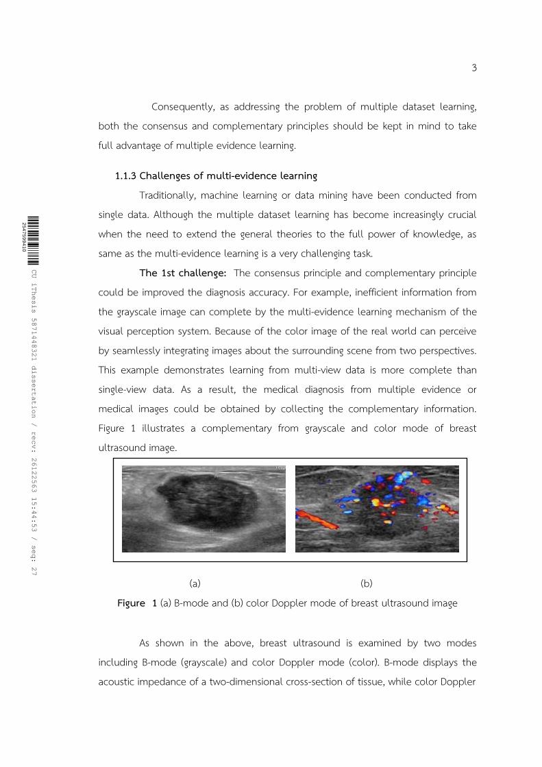
The 1st challenge: The consensus principle and complementary principle could be improved the diagnosis accuracy. For example, inefficient information from the grayscale image can complete by the multi-evidence learning mechanism of the visual perception system. Because of the color image of the real world can perceive by seamlessly integrating images about the surrounding scene from two perspectives. This example demonstrates learning from multi-view data is more complete than single-view data. As a result, the medical diagnosis from multiple evidence or medical images could be obtained by collecting the complementary information. Figure 1 illustrates a complementary from grayscale and color mode of breast ultrasound image.
(a) (b) Figure 1 (a) B-mode and (b) color Doppler mode of breast ultrasound image
As shown in the above, breast ultrasound is examined by two modes including B-mode (grayscale) and color Doppler mode (color). B-mode displays the acoustic impedance of a two-dimensional cross-section of tissue, while color Doppler
25
47
59
94
10

CU iThesis 5871448321 dissertation / recv: 26122563 15:44:53 / seq: 27
4
mode displays blood flow, the motion of tissue over time, the location of blood, the presence of specific molecules, the stiffness of tissue, or the anatomy of a three-dimensional region. The complementary information from multiple data, especially when the weaknesses of one data are complemented by the strengths of others, the complete pattern could be obtained.
Other example, learning from multiple data can reduce the noise or can avoid the missing information. Figure 2 illustrates a missing example in breast mammogram image.
Figure 2 missing example in breast mammogram image
As shown in the above, breast mammography is examined by two views including a side view (MLO) and top view (CC) of the breast. The missing lesion is appearing in the CC view, but it can be seen in the MLO view. Therefore, the missing information can be avoided when using multiple datasets.
For the convenience of joint analysis, modeling multi-evidence is required. The challenge is “How to model multiple data in a proper way is a basic issue in multi-evidence learning?”
The 2nd challenge, the relationships among datasets are important in many applications. Then such a strategy can potentially identify the relationships between multiple datasets and evaluate their learning capabilities. The particularly useful in this problem when collecting the correlated data but collecting the
25
47
59
94
10

CU iThesis 5871448321 dissertation / recv: 26122563 15:44:53 / seq: 27
5
correlated data from multiple sources may be resource-demanding and thus expensive. Sometimes, the dataset from multiple sources is uncorrelated but it useful for complementary information. Therefore, how to create their relationship to facilitate multi-evidence learning is still a challenging problem.
The 3rd challenge, dimension reduction of a huge dataset is considered. In practical applications, both the number of objects and the number of features is growing at a rapid rate. The dimension reduction methods seem an essential step for further analysis. Then, how to implement the dimension reduction becomes a challenging issue.
In this Thesis, the above challenge will be performed respectively. Meanwhile, we focus on complementary information based on the subspace learning method to apply with multi-evidence learning in medical diagnosis.
1.2 Combination of multi-evidence data 1.2.1 Subspace Learning
Subspace learning of multiple dataset learning aims to obtain a latent subspace which generated and shared by multiple evidence data. This latent subspace dimension is lower than any input data to reduce the large dimension for convenient classification or clustering tasks. In reviewing the literature on multiple dataset learning, we find that it is tightly connected with other topics in machine learning. For example, the multi-view metric learning proposed by Quadrianto and Lampert (2011) [5] and Zhai et al. (2012) [6] constructs the embedding projections from multiple datasets to shared subspace. Chen et al. (2010) [7] applied Markov network to construct the connections between the two datasets through latent subspaces. Salzmann et al. (2010)[8] and Jia et al. (2010) [9] found a latent subspace in the information by correctly factorized into shared and private parts across different datasets. Domain adaptation problem which the source domain and the target domain seen as different views can be solved by cross-language text classification [10, 11]. In addition, multi-view majority voting and multi-view co-classification [12] have been designed and successfully applied latent subspace for this problem.
25
47
59
94
10

CU iThesis 5871448321 dissertation / recv: 26122563 15:44:53 / seq: 27
6
Correlation between views is an important consideration in subspace-based approaches for multiple dataset learning. Traditionally, subspace learning using canonical correlation analysis (CCA) has been widely applied in multiple dataset learning. Hotelling (1936) [13] introduced canonical correlation analysis (CCA) to explore the linear relation between two variable sets by mutually maximizing the correlations. Several measures of association in the literature are constructed as functions of the correlation coefficients. The maximal correlation was widely selected for the next tasks.
1.2.2 Extended subspace learning Supervised-CCA: In many studies, the original CCA is extended in many
algorithms. The most extended is supervised CCA, in which one view is derived from the data and another view is derived from the class labels. Sharma et al. (2012)[14] proposed a Generalized Multi-view Analysis (GMA) which exploits supervised and unsupervised feature extraction techniques. This algorithm can potentially replace CCA whenever classification or retrieval label information. Zhai et al. (2012) [15] proposed a new semi-supervised method called Multi-view Metric Learning with Global consistency and Local smoothness (MVML-GL). This method established the relationship between data and pairs of labeled instances and shared latent space for unlabeled and test data. LEE et al. (2015) [16] presented a new method called supervised Multi-view Canonical Correlation Analysis (sMVCCA). sMVCCA utilizes a closed-form solution for determining the optimal separable and low dimensional representation via simultaneous correlation between all pairs of modalities and between each modality with the label information. This study demonstrated that the ability of sMVCCA to perform statistically significantly better in classification AUC compared to other data fusion methodologies.
MI-CCA: In reviewing the literature on extended CCA demonstrate that the supervised CCA is useful for multiple datasets learning not only reducing the data dimension but also improving the performance. However, the class labels may have appeared only on one dataset. Therefore, the CCA including the mutual information is introduced in a supervised CCA approach when the class labels have
25
47
59
94
10

CU iThesis 5871448321 dissertation / recv: 26122563 15:44:53 / seq: 27
7
appeared both datasets. Liu and Yuen (2011) [17] introduced two new confidence measures, namely, inter-view confidence and intra-view confidence using mutual information between the latent distribution and the class labels. Inspired by their success, this study proposes the mutual information including canonical correlation analysis (MI-CCA) which handles the multiple evidence of the medical diagnosis. This is distinct from previous work. First, the dataset has own class labels. Second, the mutual information is separately measured to explore the appropriate feature sets followed by CCA tasks.
1.2.3 Overview of multi-evidence learning strategies Overview: The contribution of this study aims to fuse multiple evidence
image for breast cancer diagnosis including (a) feature extraction from breast image including breast ultrasound and mammography using CNN, (b) extension of CCA via Mutual Information MI-CCA for data fusion, and (c) building a classifier model to distinguish breast tumor from benign and malignant.
Feature extraction using Convolution Neuron Network (CNN) : The features were automatically extracted by using Convolutional Neural Networks (CNN) which is powerful models that achieve impressive results for image classification to avoid the cost hand-crafted feature extraction [18]. The success from many studies [19-22] was applied to large-scale image and video recognition. Inspired by their success, this approach was used to extract the features from breast images. Bengio and LeCun suggested that complicated functions could be represented by high-level abstractions when used deep architectures, but the effective depth layers also affect to the learning time.
Extended CCA using mutual information (MI-CCA): CCA performs to maximize cross-correlation between datasets. Nevertheless, these representations do not consider the class labels of individual data. Therefore, supervised dimension reduction methods supervised-PCA and supervised-CCA are introduced [16, 23]. These studies reported that the supervised method is able to fuse data from any number of modalities to a joint subspace that can improve the model performance.
25
47
59
94
10

CU iThesis 5871448321 dissertation / recv: 26122563 15:44:53 / seq: 27
8
1.3 Contributions of this dissertation 1.3.1 Breast ultrasound image
Ultrasound (US) has been used in screening as a supplementary tool especially in women with dense breast tissue [24]. The most abnormal breast lesions are easy to find by using the conventional ultrasound, while some lesions are still hidden. Therefore, multiple ultrasound modes have been performed to extract different information from breast lesions. For example, B-mode (Brightness) displays the acoustic impedance of a two-dimensional cross-section of tissue, while color Doppler mode displays blood flow, the motion of tissue over time, the location of blood, the presence of specific molecules, the stiffness of tissue, or the anatomy of a three-dimensional region.
In previous studies, a single ultrasound mode has been individually improved. For instance, non-mass lesions were defined in four types[25]. It could be improved positive predictive values but the differentiation of NMLs by B-mode remained ambiguous and need further exploration. After intensive researches, elastography mode was well-established in cases of breast masses[26, 27]. Guo et al. [28] used of contrast agents CEUS to depict the microcirculation of breast masses and provide qualitative and quantitative analysis for classifying breast lesions. These studies showed that elastography mode could be helpful, but they note that it remained imprecise in interpretation. Color Doppler mode, which used to supplement in the conventional ultrasound, showed high sensitivity, low angle dependency, and no aliasing [29]. Nevertheless, the compilation with recent clinical research [30] reported that the Doppler image alone was not significantly distinguished from a solid mass.
Although previous studies demonstrated that single ultrasound mode could improve the overall accuracy, these investigations have some limitation. Consequently, multiple ultrasound modes have been widely combined with improving diagnosis performance. When B-mode was always examined together with color Doppler mode, the fusion of B-mode and color Doppler mode was performed [31, 32]. These studies reported that combining the B-mode and color Doppler mode showed high accuracy and specificity. Laurence R. et al. [31] evaluated the
25
47
59
94
10

CU iThesis 5871448321 dissertation / recv: 26122563 15:44:53 / seq: 27
9
performance fusion of B-mode, color Doppler, and SWE measurements. The result could significantly (p < 0.001) improved characterization of testicular masses and, therefore, could avoid inappropriate total orchiectomy.
Although previous studies demonstrated that the combination of ultrasound modes could improve the overall accuracy, these investigations were interpreted by the radiologist. According to Jeongmin Lee et al, [32] investigated the effect of automatic breast lesion detection. When inexperienced radiologists described and categorized breast lesions, especially in comparison with experienced radiologists, the automatic breast lesion detection can be more beneficial and educational for less experienced radiologists than for experienced radiologists not only describing lesions but also determining if the lesion is malignant.
Therefore, this study aims to combine the B-mode and color Doppler mode for modeling the breast cancer classification with improving diagnosis performance.
Data Acquisition and Data Description: The experiment dataset has been provided by the Department of Radiology of Thammasat University and Queen Sirikit Center of Breast Cancer of Thailand. These lesion images consisted of 53 benign lesions and 202 malignant lesions (including 255 B-mode images and 255 color Doppler mode images). The patients’ information has been removed from the images. All lesions were confirmed by biopsy; thus, it is absolutely clear whether the lesion was malignant or benign. In addition, the lesion was classified by three leading experts as malignant or benign. The consensus decision has been obtained by the majority voting rule (two out of three). The image was obtained by a Philips iU22 ultrasound machine in resolution ranges from 200×200 to 300 ×400 pixels based on the criteria of the provider. Figure 1.1 shows the different characteristics between B-mode and color Doppler mode.
1.3.2 Breast mammography image Mammography has been widely used for early screening that comprises of
Medio Lateral oblique view (MLO) and Cranio Caudal view (CC). Two views are always examined and classified in benign or malignant lesions by the radiologist. Well-trained radiologists have been found that some common pitfalls appeared in CC
25
47
59
94
10
CU iThesis 5871448321 dissertation / recv: 26122563 15:44:53 / seq: 27
10
view, whereas some pitfalls appeared in MLO view [33]. Single view and two-view mammographic examinations interpreted by experienced radiologists were compared in many studies [34-36]. These studies reported that two-view screening could improve the cancer detection rate. Then, they suggested that other methods may be reduced missing such as explored correlation of image or integrated of double reading. The study in breast positioning explained that CC-view and MLO-view are different point of each view.
According to previous reports, multi-views in mammography tend to avoid missed interpretation. Vijayarajan and Jaganathan (2014) [37] proposed transform 2D to 3D feature of MLO and CC view, then, the features were combined 3D boundary features of two views. Several recent studies[38, 39] worked with feature extraction using Convolutional Neuron Networks (CNNs) to share relevant features between MLO and CC view and improve model performance.
Data Acquisition and Data Description: Breast mammographic digitized images published from the Digital Database for Screening Mammography (DDSM) has been widely used as a benchmark for numerous studies on the mammographic area. These datasets consist of 600 CC-view and 600 MLO-view and compose of 200 normal, 200 benign, and 200 malignant for each view. Each image has a resolution of 256×514 pixels gray level tones.
1.3.3 The contributions of dissertation 1.3.3.1 When The consensus principle and complementary principle could
be improved the diagnosis accuracy, this study proposes the data fusion approach to employ comprehensively and accurately describe the data by using the data that may contain some knowledge that other evidence does not have.
1.3.3.2 Also, we propose the supervised feature selection explored the mutual information between related feature and class label. The output features of the last convolutional layer were reduced before the fusion process.
1.3.3.3 Information fusion using canonical correlation analysis is performed to combine multi-evidence features (multiple ultrasound modes or multiple mammography views). Each feature provides an independent, but it could be
25
47
59
94
10

CU iThesis 5871448321 dissertation / recv: 26122563 15:44:53 / seq: 27
11
complemented observation of the instances and thus we implement CCA on their combination to seek a joint mapping, which is useful for detecting breast lesions and distinguishing breast cancer.
25
47
59
94
10

CU iThesis 5871448321 dissertation / recv: 26122563 15:44:53 / seq: 27
Chapter II
Primarily theories 2.1 Primarily theories
2.1.1 Feature Extraction This section is dedicated to the description of NN in general and its special
type called CNN that use for feature extraction.
2.1.1.1 Neural Networks NNs is the invention of Perceptron inspired by Biology of central
nervous systems of mammals. Perceptron used the biological neuron that also described an algorithm for direct learning from data. It resembles the brain in two respects. First, the knowledge is acquired by the network from its environment through a learning process. Second, the strength connection of neuron, known as synaptic weights, are used to store the acquired knowledge. When NNs are used for classification problems, it interprets the outputs as probabilities of the inputs belonging to each class. For example, the inputs (x1, x2) are the coordinates, and the output (y0, y1) is constant, which sums to 1. The decision boundary is chosen. This means that when y0 > y1 the algorithm will classify the data point as 0 and vice versa. The schematic representation can be seen in figure 3.
Figure 3 Schematic representation of a simple perceptron.
φ(x) Σ y Output
25
47
59
94
10

CU iThesis 5871448321 dissertation / recv: 26122563 15:44:53 / seq: 27
13
X1
X2 0 1
1
X1
X2 0 1
1
?
Input variables xi, corresponding weights wi, the weighted sum of the inputs, an activation function φ, the output y and the bias b. Bias is an additional input to each neuron often represented as an input x = 1 and a weight w0 (w0 =
b). The output y from the single perceptron is:
𝑦 = 𝜑 (∑ 𝑤𝑘𝑥𝑘 + 𝑏
𝑚
𝑘=1
)
Including the bias in the summation we get:
𝑦 = 𝜑 (∑ 𝑤𝑘𝑥𝑘
𝑚
𝑘=0
)
𝜑 is called an activation function. A sigmoid function is often used for regular NNs, as the logistic function or tan(x). When working with CNNs, the Rectified Linear Unit (ReLU) is mostly used to extract the features. It is defined as:
𝜑(𝑥) = {0 𝑖𝑓 𝑥 ≤ 0,𝑥 𝑖𝑓 𝑥 > 0.
The decision boundary is a hyperplane that is linearity (cf. linear SVM). With a single perceptron, it may solve the AND and OR problem.
(a) (b) Figure 4 (a) AND problem (b) XOR problem
25
47
59
94
10

CU iThesis 5871448321 dissertation / recv: 26122563 15:44:53 / seq: 27
14
Figure 4 shows a simple perceptron that is very promising to separate linearly problems. However, among other studies contained mathematical proof that perceptron is unable to solve simple XOR problem [40]. Therefore, NNs was shown that any complex problems could have been solved by usage of multiple perceptron units. The invention of the back-propagation learning algorithm was introduced to gather neurons into groups called layers which can be stacked into hierarchical structures to form a network called Multilayer Perceptron (MLP).
Figure 5 Schematic representation of a Multilayer Perceptron.
Figure 5 has classified the output 𝑦𝑖 for the input 𝑥𝑖. The function for calculating these outputs is:
𝑦𝑖 = 𝜑0 (∑𝑤𝑖𝑗𝜑ℎ (∑ �̃�𝑗𝑘𝑥𝑘
4
𝑘=0
)
5
𝑖=0
)
In the final classification, softmax function is commonly used
to get 𝑦𝑖 from the probability that belongs to class i. Deep Neural Networks or deep learning are also performed to increase the depth of the network. When adding hidden layers, the decision boundary is not limited to a hyperplane.
25
47
59
94
10

CU iThesis 5871448321 dissertation / recv: 26122563 15:44:53 / seq: 27
15
2.1.1.2 Convolutional Neural Networks Convolutional Neural Network (CNN) is a neural network that
composes of deep neural layers. Due to further application in image analysis, the use of CNNs is widely used as medical images.
Structure: Convolutional Neural Network consists of the hidden layers that have different configurations. A filter of spatial neurons takes input images and presents the probability of each class as output. A schematic representation of a Convolutional Neural Network can be seen in figure 6, and below explain the different layers.
Figure 6 Schematic representation of a Convolutional Neural Network.
Convolutional layer: Convolution is a major part of the function of these networks, a function x with a kernel w in two dimensions is defined as:
𝑆(𝑖, 𝑗) = ∑∑𝐼(𝑚, 𝑛)𝐹(𝑖 − 𝑚, 𝑗 − 𝑛),
𝑛𝑚
The filter (F) up-down and left-right and sum over all products.
25
47
59
94
10

CU iThesis 5871448321 dissertation / recv: 26122563 15:44:53 / seq: 27
16
Original image CNN Result Filter
Figure 7 An example showing how convolution of an image works. An example can be seen in the top picture in figure 7. The
marked pixels will calculate of the convolution at this point:
𝐼𝑛𝑝𝑢𝑡 𝑝𝑖𝑥𝑒𝑙 = [9 60 1
] , 𝐹𝑖𝑙𝑡𝑒𝑟 = [1 00 −1
] The results is:
(1)(9) + (0)(6) + (0)(0) + (1)(−1) = 8
Pooling layer: Pooling layers cause a down-sampling of the filter outputs. Max-pooling, which the largest value within this filter is saved to the next layer, is mostly used in CNN network. Thus, the largest information of image will save and move to do the next calculation.
Figure 8 the principle of max-pooling.
25
47
59
94
10

CU iThesis 5871448321 dissertation / recv: 26122563 15:44:53 / seq: 27
17
Fully-connected Layer: Neurons in a fully connected layer have full connections to all activations in the previous layer. A matrix multiplication followed by a bias offset is computed with their activation.
The most common architecture stacks compose of a few CONV-RELU layers, follow them with POOL layers, and repeat this pattern until the image has been merged spatially to a small size. The class scores are calculated from the last fully-connected layer. Furthermore, other layer such as Normalization layer or Dropout layer have been introduced to improve the model performance.
2.1.2 Feature Selection Feature Selection is the process of selecting what inputs should be
presented to a classification algorithm. Generally, the feature selection was performed by domain experts, while modern classification approaches attempt to collect all possible features and then use a statistical feature selection process to determine which features are relevant for the classification problem. The feature set contains irrelevant (week information about the classification problem) and/or redundant (already present in more informative features). Both irrelevant and redundant are increase the collection cost of the feature set. In addition, shrinking the feature set also improve classification performance. These heuristic notions of relevancy and redundancy were formalized by Kohavi & John [41] into three classes: strongly relevant, weakly relevant, and irrelevant. The strongly relevant features contain useful information, while the weakly relevant features contain weak information, then, the irrelevant features contain no useful information about the problem. Therefore, the ideal feature selection algorithm would return the set of strongly relevant features excluding the irrelevant features. In chapter 2.1.1, the feature extraction was performed and returned the set of strongly relevant features, subset of the weakly relevant features, and including the irrelevant features.
25
47
59
94
10

CU iThesis 5871448321 dissertation / recv: 26122563 15:44:53 / seq: 27
18
Feature selection algorithm are three main kinds: filters, wrappers, and embedded methods. This chapter will focus on filters algorithms. Filters algorithm is the evaluation function or criterion which scores the utility of a feature or a feature set, and the search algorithm which generates new candidate features or feature sets for evaluation.
2.1.2.1 Filters algorithm Filter approaches use a measure of relevancy or separation
between the candidate feature or feature set and the class label by scoring a feature or feature set. These measures range from simple correlation measures such as Pearson's Correlation Coefficient [42], through complex correlation measures such as the mutual information (discussed in Section 2.1.3). All these measures achieve to return the strong relationship between the candidate feature set and the class label. This relationship might be a measure of probabilistic independence. This thesis calls mutual information scoring (MI score) based on information theoretic measures. The scoring criteria is along with a search method to select candidate feature sets [43]. The complexity of the scoring usually enforces the complexity of the search method. Many common filters use greedy forward or backward searches [44, 45] to adding or removing each feature based on high score or low score. Branch & Bound methods [46] was improved in optimal search strategies and exclude groups of features from consideration if they can never improve in performance. However, such complex search algorithms are unnecessary in certain situations, notably in the case of univariate feature selection where the best features based on univariate statistical tests can be investigated discrete target variable.
Due to the use of abstract measures of correlation between variables and target classes, they return useful feature set which should perform well with classification algorithms.
25
47
59
94
10

CU iThesis 5871448321 dissertation / recv: 26122563 15:44:53 / seq: 27
19
2.1.3 Mutual Information 2.1.3.1 Information Theory
The relationship between two variables can measure the amount of shared information between two variables. Information Theory has been performed to measure the amount of shared information. The uncertainty quantity of information can be reduced in one variable when another variable is known. Claude Shannon defines three crucial measures which form the basis of much of the rest of the work we present in this thesis [47].
They are the Entropy, H(X), for a random variable X, the Conditional Entropy of X given another random variable Y , H(X;Y ), and the Mutual Information between two variables, I(X; Y).
The Entropy of a random variable X , measures the uncertainty about the state of a sample x from X. The entropy of X is defined in terms of the probability distribution p(x) over the states of X as follows:
𝐻(𝑋) = − ∑ 𝑝(𝑥) log 𝑝(𝑥)
𝑥∈𝑋
The logarithm base defines the units of entropy, with log2 using bits. High values of entropy mean the state of x is very uncertain (and thus highly random), and low values mean the state of x is more certain (and thus less random), then, the uncertain state of x is the hardest to predict. The entropy of X given Y
measures the uncertainty of the state of a sample of x when Y is known. This has two equivalent definitions, in terms of the joint probability distribution p(x; y),
𝐻(𝑋; 𝑌) = ∑ 𝑝(𝑦)𝐻(𝑥; 𝑌 = 𝑦)
𝑦∈𝑌
= − ∑ ∑ 𝑝(𝑥, 𝑦)log 𝑝(𝑥; 𝑦)
𝑥∈𝑋𝑦∈𝑌
The conditional entropy investigates the interaction between
two variables. When knowing the entropy of X, It can derive any useful information. This conditional entropy is called the Mutual Information, I(X; Y). It measures the
25
47
59
94
10

CU iThesis 5871448321 dissertation / recv: 26122563 15:44:53 / seq: 27
20
reduction in uncertainty in the state of X when the state of Y is known and increase in the relevant information. This leads to several equivalent definitions for the mutual information,
𝐼(𝑋; 𝑌) = 𝐻(𝑋) − 𝐻(𝑋; 𝑌)
= 𝐻(𝑌) − 𝐻(𝑌; 𝑋)
= 𝐻(𝑋) + 𝐻(𝑌) − 𝐻(𝑋𝑌)
The mutual information can also be expressed as the relative entropy between the joint distribution p(x; y) and the product of both marginal distributions p(x)p(y), defined as follows:
𝐼(𝑋; 𝑌) = ∑ ∑ 𝑝(𝑥, 𝑦)log (𝑝(𝑥, 𝑦)
𝑝(𝑥)𝑝(𝑦))
𝑥∈𝑋𝑦∈𝑌
With this formulation can investigate the mutual information reaches its maximal and minimal values. The maximal value is the minimum of the two entropies H(X) and H(Y), and occurs when knowledge of one variable allows perfect prediction of the state of the other. The minimal value is 0, which occurs when X and Y are independent. When knowing of one variable (and the condition of variable), It allows the perfect prediction. This study will use of the conditional mutual information in feature selection task.
2.1.3.2 Estimating the mutual information Mutual information calculation can estimate using entropy
estimation and estimate probability distributions. Paninski [48] shows the detail of this topic. This section provides a brief summary of the relevant issues and notations. The mutual information as the expected logarithm of a ratio of probabilities:
𝐼(𝑋; 𝑌) = 𝐸𝑥𝑦 {𝑙𝑜𝑔𝑝(𝑥, 𝑦)
𝑝(𝑥)𝑝(𝑦)}
Then �̂� denote a probability distribution which has been estimated from a dataset sampled from the true distribution p. The sample estimate using �̂� converges to the expected value N observations (𝑥𝑖 , 𝑦𝑖):
25
47
59
94
10
CU iThesis 5871448321 dissertation / recv: 26122563 15:44:53 / seq: 27
21
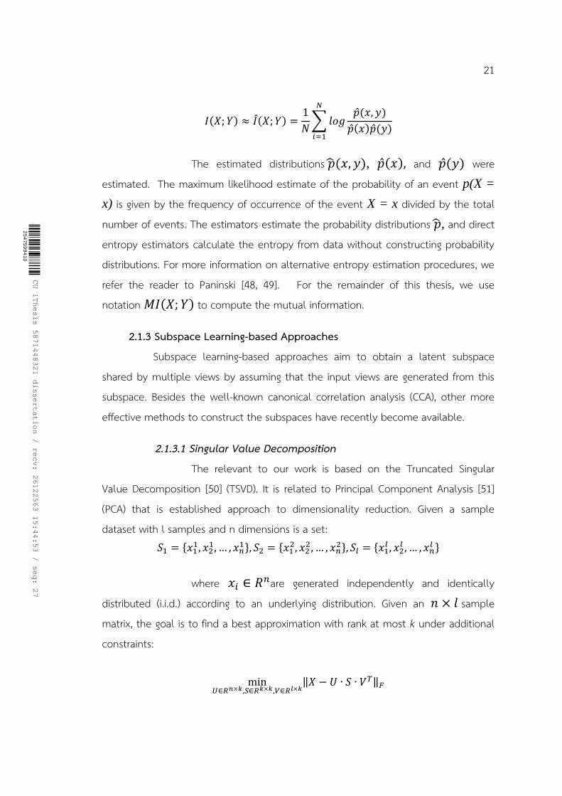
𝐼(𝑋; 𝑌) ≈ 𝐼(𝑋; 𝑌) =1
𝑁∑𝑙𝑜𝑔
�̂�(𝑥, 𝑦)
�̂�(𝑥)�̂�(𝑦)
𝑁
𝑖=1
The estimated distributions �̂�(𝑥, 𝑦), �̂�(𝑥), and �̂�(𝑦) were estimated. The maximum likelihood estimate of the probability of an event p(X =
x) is given by the frequency of occurrence of the event X = x divided by the total number of events. The estimators estimate the probability distributions �̂�, and direct entropy estimators calculate the entropy from data without constructing probability distributions. For more information on alternative entropy estimation procedures, we refer the reader to Paninski [48, 49]. For the remainder of this thesis, we use notation 𝑀𝐼(𝑋; 𝑌) to compute the mutual information.
2.1.3 Subspace Learning-based Approaches Subspace learning-based approaches aim to obtain a latent subspace
shared by multiple views by assuming that the input views are generated from this subspace. Besides the well-known canonical correlation analysis (CCA), other more effective methods to construct the subspaces have recently become available.
2.1.3.1 Singular Value Decomposition The relevant to our work is based on the Truncated Singular
Value Decomposition [50] (TSVD). It is related to Principal Component Analysis [51] (PCA) that is established approach to dimensionality reduction. Given a sample dataset with l samples and n dimensions is a set:
𝑆1 = {𝑥11, 𝑥2
1, … , 𝑥𝑛1}, 𝑆2 = {𝑥1
2, 𝑥22, … , 𝑥𝑛
2}, 𝑆𝑙 = {𝑥1𝑙 , 𝑥2
𝑙 , … , 𝑥𝑛𝑙 }
where 𝑥𝑖 ∈ 𝑅𝑛are generated independently and identically
distributed (i.i.d.) according to an underlying distribution. Given an 𝑛 × 𝑙 sample matrix, the goal is to find a best approximation with rank at most k under additional constraints:
min
𝑈∈𝑅𝑛×𝑘,𝑆∈𝑅𝑘×𝑘,𝑉∈𝑅𝑙×𝑘‖𝑋 − 𝑈 ∙ 𝑆 ∙ 𝑉𝑇‖𝐹
25
47
59
94
10

CU iThesis 5871448321 dissertation / recv: 26122563 15:44:53 / seq: 27
22
Subject to 𝑈𝑇𝑈 = 𝐼𝑘
𝑉𝑇𝑉 = 𝐼𝑘
𝑆 = 𝑑𝑖𝑎𝑔(𝜎), 𝜎 ∈ 𝑅𝑘, 𝜎𝑖 ≥ 0
The PCA is based on a low rank decomposition of the empirical covariance matrix and computed based on the sample matrix. The main idea is to find a subspace that accounts for as much as variability in the data as possible. The first principal component is defined as the one-dimensional subspace that maximizes the variance of the data when projected onto it. Formally, it solves the following problem:
max 𝑢∈𝑅𝑛
𝑉𝑎𝑟(𝑢𝑇 ∙ 𝑋),
Subject to ‖𝑢‖ = 1
The other principal vectors can be solved the eigenvalue problem:
min𝑈∈𝑅𝑛×𝑘
‖𝐶𝑜𝑣(𝑋) − 𝑈 ∙ Ʌ ∙ 𝑉𝑇‖𝐹
One of the main applications of PCA is as a dimensionality reduction technique. The data is projected to the space spanned by the normalized eigenvectors (also called principal vectors). In general applications, an eigenvalue decomposition is used and discarded the principal vectors with small eigenvalues (similar to SVDs).
2.1.3.2 Canonical Correlation Analysis Canonical Correlation Analysis (CCA) [52] is a general procedure
for finding the relationships between two sets of random variables based on analyzing the cross-covariance matrix. CCA aims to identify linear relationships between two random vectors. Given two random vectors 𝑋1and 𝑋2 are in pair of function 𝑓(1)and 𝑓(2)such that there is linear dependence between 𝑓(1)(𝑋1) and 𝑓(2)(𝑋2), that is, 𝑓(1)(𝑋1) should share some information for 𝑓(2)(𝑋2). This enables applications such as cross-modal information retrieval, classification, clustering, etc.
25
47
59
94
10

CU iThesis 5871448321 dissertation / recv: 26122563 15:44:53 / seq: 27
23
For example, if 𝑓(1) encodes a visual image and 𝑓(2) encodes a textual description of the scene, text input based on search over a collection of images was performed using cross-modal shared information [53]. Bi-lingual document analysis is another application, see[54, 55].
The idea is to find two vectors 𝑤1 ∈ 𝑅𝑝 and 𝑤2 ∈ 𝑅𝑞 so that the random variables 𝑤1
𝑇 ∙ 𝑋1 and 𝑤2𝑇 ∙ 𝑋2 are maximally correlated (𝑤1
𝑇and 𝑤2𝑇 map
the random vectors to random variables, by computing weighted sums of vector components). By using the sample matrix notation 𝑋1and 𝑋2 this problem can be formulated as the following optimization problem:
𝜌 = maximize𝑤1∈𝑅𝑝,𝑤2∈𝑅𝑞
𝑤1𝑇𝐶𝑜𝑣(𝑋1, 𝑋2)𝑤2
√(𝑤1𝑇𝐶𝑜𝑣(𝑋1)𝑤1)(𝑤2
𝑇𝐶𝑜𝑣(𝑋2)𝑤2)
where 𝐶𝑜𝑣(𝑋1) and 𝐶𝑜𝑣(𝑋2) are estimated of variances of
𝑋1and 𝑋2, and 𝐶𝑜𝑣(𝑋1, 𝑋2) is covariance between 𝑋1and 𝑋2. The optimization problem can be solved to a generalized eigenvalue problem [55]:
[0 𝐶𝑜𝑣(𝑋1, 𝑋2)
𝐶𝑜𝑣(𝑋2, 𝑋1) 0] ∙ [
𝑤1
𝑤2] = 𝜆 ∙ [
𝐶𝑜𝑣(𝑋1, 𝑋1) 0
0 𝐶𝑜𝑣(𝑋2, 𝑋2)] ∙ [
𝑤1
𝑤2]
Or
[𝐶22−1𝐶21𝐶11
−1𝐶12 − 𝜆𝐼]𝑤𝑖 = 0
where 𝐶11 , 𝐶22, and 𝐶12 are covariance matrix of the features 𝑋1
and 𝑋1, 𝑋2 and 𝑋2, then 𝑋1 and 𝑋2, and I is the identity matrix. A single canonical variable is usually inadequate in representing
the original random vector and typically one looks for k projection pairs (𝑤1
1, 𝑤12),…, (𝑤𝑘
1, 𝑤𝑘2), so that 𝑤𝑖
1 and 𝑤𝑖2 are highly correlated. This problem can be
formulated as a symmetric eigenvalue problem.
25
47
59
94
10

CU iThesis 5871448321 dissertation / recv: 26122563 15:44:53 / seq: 27
Chapter III
Methodology 3.1 Overview proposed methodology
The contribution of this study aims to fuse multiple evidence for breast cancer diagnosis. The proposed method is including (a) feature extraction from breast images using CNN, (b) feature selection using mutual information that is extension of CCA (c) CCA for data fusion, and (d) building a classifier model to distinguish breast tumor from benign and malignant. Figure 9 shows the overview of method.
Figure 9 MI-CCA architecture model
The runner-up in ILSVRC 2014 [56] showed the depth of the network that was a
critical component for good performance. However, training a deep CNN often
requires computational resources. To address these challenges, transfer learning [57]
is introduced to pre-trained followed by a specific task. The architecture of VGGNet
was used to extract the features for breast ultrasound and mammography images
followed by top-layer. There are three steps for extracting the image feature. First,
25
47
59
94
10

CU iThesis 5871448321 dissertation / recv: 26122563 15:44:53 / seq: 27
25
the input of each modes is fed to VGGNet backbone without fully training. Second,
the output features from VGGNet layer are trained using CNN top-layer. Finally, the
backpropagation process is performed only with CNN top-layer. Proposed model
architecture consists of two parts that show in Figure 13.
3.2 Feature extraction 3.2.1 Software Tools
There are many software tools for machine learning. Almost every commonly used programming language has either some software library or at least some available Application Programming Interface (API). Keras written in python and high-level neural network API was used for this study. It is very simple with rapid model development and good documentation containing many code examples to get started very quickly.
3.2.2 Hardware and Software Configuration
Training of CNN demands a lot of resources and converts into many multiplications of matrices. Central Processing Units (CPUs) are not sufficient for computations. On the other hand, modern GPUs are designed to perform these operations. An efficient GPU in Keras is relying on either Theano or Tensorflow back-end.
3.2.3 Dataset Preparation The CNN model imposed the constraint that each image has to be of the
same size and aspect ratio. Then, dataset preparation was done in three stages. Image generator using keras library: The field of machine learning
encounters a situation where the model tries to load a dataset but there is not enough memory. This is already one of the challenges in the field of vision where large datasets of images and video files are processed. To address this problem, keras supports data generators for loading and processing images. The ImageDataGenerator class is an easy way to load and augment images in batches for image classification tasks.
25
47
59
94
10

CU iThesis 5871448321 dissertation / recv: 26122563 15:44:53 / seq: 27
26
Split data into training and testing dataset: Images are randomly split between train and test dataset. It is very important that both datasets should be having an equal split among the categories because the imbalance category would be biased to the major category. This was caused by the fact that medical image was hard to collect equally classes. It was solved by kernel-based methods during random selection.
3.2.4 Model building blocks For the implementation of CNN using Keras, the sequential model is
appropriate for modeling of the feed-forward network. Definition of the network is composed of multiple Keras layers. All models were created by composition of following layers.
Convolutional: Convolutional layer used in the architecture was of following structure
Conv2D(filters=n, kernel_size=(z, z), strides=(s, s),
padding=’valid’, input_shape=shape)
where n is number of filters that the layer will have, 𝑧 is size of kernel, 𝑠 is number of pixels in stride and input_shape defines size of input matrix.
Activation: The activation function was added to the output of the layer.
Activation(acitvation_function)
where activation_function is either “softmax” or “relu”. Both specifications are equivalent because Keras automatically uses linear activation function for each layer.
Pooling: Pooling layer can be specified as
MaxPooling2D(pool_size=(z, z), strides=(s, s))
where pool_size specifies size of pooling kernel and strides specifies number of pixels in x and y direction that are traversed in between application of individual pools.
25
47
59
94
10

CU iThesis 5871448321 dissertation / recv: 26122563 15:44:53 / seq: 27
27
Flatten: Feature extraction layers are multidimensional. Specifically, both Convolutional and Pooling layers are two dimensional. Classification layers that are created by fully connected layers are one dimensional. Then, flatten is necessary to create mapping between them.
Flatten()
3.2.5 Model Compilation and fitting Model Compilation: Before trained the model, it needs to have cost
function, optimization procedure and metrics defined. This is done by compiling the model.
model.compile(
loss= ’categorical_crossentropy’,
optimizer=Adam(lr=0.001),
metrics=[’accuracy’])
parameter loss specifies cost function, optimizer optimization procedure and metrics specifies metrics by which the model is measured.
Model fit: Process of model training is in Keras called model fitting.
model.fit([train_data1, train_data2], train_labels,
batch_size=batch_size, epochs=epoch_num,
shuffle=True, verbose=0,
validation_data=([valid_data1, valid_data2],
valid_labels))
3.3 Feature selection using mutual information
The MI between random variables 𝑋 and 𝑌 can be estimated the under-probability distribution form posterior knowledge of the pointwise mutual information 𝐼(𝑋; 𝑌). If X given Y are the evens, then the true frequencies of all combinations of (𝑋; 𝑌) pairs can estimate by counting the number of times each pair occurs in the data.
The mutual information scores were computed using the equation, shown as:
25
47
59
94
10

CU iThesis 5871448321 dissertation / recv: 26122563 15:44:53 / seq: 27
28
𝐼(𝑋; 𝑌) = ∑ ∑ 𝑝(𝑥, 𝑦)log (𝑝(𝑥, 𝑦)
𝑝(𝑥)𝑝(𝑦))
𝑥∈𝑋𝑦∈𝑌
(1)
where 𝑝(𝑥, 𝑦) is the joint probability density function of 𝑋 and 𝑌, and 𝑝(𝑥)𝑝(𝑦) are the marginal probability density functions of 𝑋 and 𝑌 respectively. If 𝑋 and 𝑌 are independent, then knowing 𝑋 does not give any information about 𝑌, their mutual information is zero. Followed by this concept the parametric distributions over feature and target class, it is convenient to revise from the equation (1), shown as:
𝐼(𝑓(∙); 𝑌) = ∑ ∑𝑝(
𝑦𝜖𝑌𝑓(∙)∈𝑋
𝑓(∙); 𝑌) log (𝑝(𝑓(∙); 𝑌)
𝑝(𝑓(∙))𝑝(𝑌)) (2)
where the set of 𝑓(∙) is final output from CNNs networks, and 𝑌 is the possible
target class. The mutual information scores:
𝐼1(𝑓(𝑥1); 𝑌), 𝐼2(𝑓(𝑥2); 𝑌), … , 𝐼𝑖(𝑓(𝑥𝑖); 𝑌)
An information theoretic filter algorithm is one that uses a measure drawn from Information Theory (such as the mutual information we described in Chapter 2) as the evaluation criterion. Evaluation criteria are designed to measure how useful a feature or feature subset is when used to construct a classier. We will use 𝑀𝐼𝑠𝑐𝑜𝑟𝑒 to denote an evaluation criterion which measures the performance of a feature or set of features. The most evaluation criteria in information theoretic feature selection is selecting the feature with the highest mutual information to the class label 𝑌. shown as: 𝑀𝐼𝑠𝑐𝑜𝑟𝑒𝑖
= 𝐼𝑖(𝑓(𝑥𝑖); 𝑌) (3)
We refer to this feature scoring criterion as “score”, standing for mutual
information which considers a score for each feature independently of others. This criterion is very simple, and thus it can replace conditions in the search algorithm. This is a univariate measure, and each feature's score is independent of the other
selected features. If we wish to select k features using 𝑀𝐼𝑠𝑐𝑜𝑟𝑒 will pick the top k features, ranked according to their mutual information with the class. We could also
25
47
59
94
10

CU iThesis 5871448321 dissertation / recv: 26122563 15:44:53 / seq: 27
29
select features until we had reached a predefined threshold of mutual information or another condition.
The proposed method was computed from equation (2). Then, the features from CNNs networks𝑓(∙) which correspond over mean score would be selected to the fusion task, shown as:
𝑓(𝑋1) = 𝑀𝐼𝑠𝑐𝑜𝑟𝑒𝑖1 ≥ 𝑚𝑒𝑎𝑛
𝑓(𝑋2) = 𝑀𝐼𝑠𝑐𝑜𝑟𝑒𝑖2 ≥ 𝑚𝑒𝑎𝑛
where superscript1 is the first dataset and superscript2 is the second dataset, respectively.
Figure 10 Mutual Information evaluation and selection This operation can be performed using sklearn.feature_selection library.
The library was used for estimating the mutual information for a continuous target variable. The function relies on nonparametric methods based on entropy estimation as described in [58] and [59]. Both methods are based on the idea originally proposed in [60].
MIscore ≥mean
25
47
59
94
10

CU iThesis 5871448321 dissertation / recv: 26122563 15:44:53 / seq: 27
30
3.4 Feature fusion using canonical correlation analysis The features from CNNs networks𝑓(∙) which correspond over 0.95 score were
selected and defined as 𝑓(𝛼1), 𝑓(𝛼2), … , 𝑓(𝛼𝑖); 𝑖 ∈ 1,2, … , 𝑛 Given pair of data samples 𝛼1
𝑖 , 𝑖 ∈ {1, 2, … , 𝑛} of the first dataset, such that 𝛼2𝑖 , 𝑖 ∈ {1, 2, … , 𝑛}, to the
second dataset respectively. Features matrix such that 𝐴1 = [𝛼11, 𝛼1
2, … , 𝛼1𝑛 ]
and 𝐴2 = [𝛼21, 𝛼2
2, … , 𝛼2𝑛 ], respectively. CCA accounts to fusion more than two
datasets based on cross correlation. Although the correlation of more than two datasets could not be easy to examine, the subspace which maximizes the correlations of each pair in sequential has been instead approximated [61]. Given n data samples comprise of features 𝐴𝑖
1, 𝐴𝑖2, … , 𝐴𝑛
𝑀, 𝑀, 𝑖 ∈ {1, 2, … , 𝑛}from M dataset and n feature, this implementation of pairwise CCA attempts a set of linear transformations 𝑤1 ∈ 𝑅𝑛1×1, 𝑤2 ∈ 𝑅𝑛2×1, … , 𝑤𝑀 ∈ 𝑅𝑛𝑀×1 such that the sum of the correlations across all pairs of modalities is maximized, show as:
𝜌 = maximize𝑤1,𝑤2
𝑤1𝑇𝐶12𝑤2
√(𝑤1𝑇𝐶11𝑤1)(𝑤2
𝑇𝐶22𝑤2)
(4)
where 𝐶11 , 𝐶22, and 𝐶12 are covariance matrix of the features 𝐴1 and 𝐴1, 𝐴2 and 𝐴2, then 𝐴1 and 𝐴2, respectively.
[𝐶11 𝐶12
𝐶21 𝐶22] =
[ 𝐶11 [
𝑐𝑜𝑣(𝛼111 ) ⋯ 𝑐𝑜𝑣(𝛼1𝑞
1 )
⋮ ⋱ ⋮𝑐𝑜𝑣(𝛼𝑝1
1 ) ⋯ 𝑐𝑜𝑣(𝛼𝑝𝑞1 )
] 𝐶12 [
𝑐𝑜𝑣(𝛼1112) ⋯ 𝑐𝑜𝑣(𝛼1𝑞
12)
⋮ ⋱ ⋮𝑐𝑜𝑣(𝛼𝑝1
12) ⋯ 𝑐𝑜𝑣(𝛼𝑝𝑞12)
]
𝐶21 [
𝑐𝑜𝑣(𝛼1121) ⋯ 𝑐𝑜𝑣(𝛼1𝑞
21)
⋮ ⋱ ⋮𝑐𝑜𝑣(𝛼𝑝1
21) ⋯ 𝑐𝑜𝑣(𝛼𝑝𝑞21)
] 𝐶22 [
𝑐𝑜𝑣(𝛼112 ) ⋯ 𝑐𝑜𝑣(𝛼1𝑞
2 )
⋮ ⋱ ⋮𝑐𝑜𝑣(𝛼𝑝1
2 ) ⋯ 𝑐𝑜𝑣(𝛼𝑝𝑞2 )
]
]
By using Lagrangian multiplier techniques one can transform the constrained optimization problem to a generalized multivariate eigenvalue problem of the form: [𝐶22
−1𝐶21𝐶11−1𝐶12 − 𝜆𝐼] = 0 (5)
[𝐶11
−1 − 𝜆 𝐶12
𝐶21 𝐶22−1 − 𝜆
] = 0
(𝐶11−1 − 𝜆)(𝐶22
−1 − 𝜆) − (𝐶21)(𝐶12) = 0
Where
𝜆 =−𝑏 ± √𝑏2 − 4𝑎𝑐
2𝑎
25
47
59
94
10

CU iThesis 5871448321 dissertation / recv: 26122563 15:44:53 / seq: 27
31
After this process, the eigenvalue 𝜆𝑖 was presented. Canonical vectors are
unknown and must be computed. [𝐶22
−1𝐶21𝐶11−1𝐶12 − 𝜆𝑖𝐼]𝑤𝑖 = 0
where 𝑖 ∈ 1, 2, … , 𝑛 is the number of datasets, for instance, if the first matrix
𝐴1 ∈ 𝑅2×2 and the second matrix 𝐴2 ∈ 𝑅2×2 , the covariant matrix are 2×2, the eigenvalue compose of 𝜆1𝑎𝑛𝑑 𝜆2, the eigenvector compose of 𝑊1 ∈ 𝑅2×2 and 𝑊2 ∈
𝑅2×2, while if we have n matrix, the covariant metric are 𝐶𝑖 ∈ 𝑅𝑛×𝑛, the eigenvalue compose of 𝜆1, 𝜆2, … , 𝜆𝑛, the weight matrix compose of 𝑊𝑖 ∈ 𝑅𝑛×𝑛.
CCA is a method for finding linear relationships between two datasets. Given
two datasets 𝑋 = (𝑥1, 𝑥2, … , 𝑥𝑛) ∈ 𝑅𝑑×𝑛 and 𝑌 = (𝑦1, 𝑦2, … , 𝑦𝑚) ∈ 𝑅𝑑×𝑚 (where 𝑥𝑖 ,
𝑦𝑖 are d-dimensional vectors), CCA finds a canonical coordinate space that maximizes
correlations between the projections of the datasets onto that space. For each
dimension of this coordinate space, there is a pair of projection weight vectors.
Therefore, it is convenient to formulate CCA as a generalized eigenvalue problem
that can be solved in one shot. The objective function (equation 4), which solves for
the maximum of the canonical correlation vector, is rewritten in terms of the sample
covariance 𝐶𝑥𝑦 of datasets X and Y and the autocovariances 𝐶𝑥𝑥 and 𝐶𝑦𝑦:
Without constraints on the canonical weights 𝑤1 and 𝑤2, the objective
function has infinite solutions. However, the size of the canonical weights can be
constrained, such that 𝑤1𝑇𝐶𝑥𝑥𝑤1 = 1, and 𝑤2
𝑇𝐶𝑦𝑦𝑤2 = 1 This constraint results in the
following Lagrangian:
𝐿(λ, 𝑤1, 𝑤2) = 𝑤1𝑇𝐶𝑥𝑦𝑤2 −
λx
2 (𝑤1
𝑇𝐶𝑥𝑥𝑤1 − 1) −λy
2 (𝑤2
𝑇𝐶𝑦𝑦𝑤2 − 1)
The objective function can then be formulated as the following generalized
eigenvalue problem:
[0 𝐶𝑥𝑦
𝐶𝑦𝑥 0] ∙ [
𝑤1
𝑤2] = 𝜌2 [
𝐶𝑥𝑥 00 𝐶𝑦𝑦
]
25
47
59
94
10

CU iThesis 5871448321 dissertation / recv: 26122563 15:44:53 / seq: 27
32
The generalized eigenvalue problem is also modified to incorporate
regularization:
[0 𝐶𝑥𝑦
𝐶𝑦𝑥 0] ∙ [
𝑤1
𝑤2] = 𝜌2 [
𝐶𝑥𝑥 + λI 00 𝐶𝑦𝑦 + λI
]
Regularized CCA is mathematically like partial least squares regression (PLS).
Compare to the objective function of CCA (Equation 4) the objective function that is
optimized in PLS:
𝜌 = maximize𝑤1∈𝑅𝑝,𝑤2∈𝑅𝑞
𝑤1𝑇𝐶𝑥𝑦𝑤2
√(𝑤1𝑇𝑤1𝑤2
𝑇𝑤2)
Analogously to CCA, PLS can be solved as a generalized eigenvalue problem:
[0 𝐶𝑥𝑦
𝐶𝑦𝑥 0] ∙ [
𝑤1
𝑤2] = 𝜌2 [𝐼 0
0 𝐼]
Once 𝑊𝑥 and 𝑊𝑦 are obtained, the projected new features, called canonical
variables, are computed by 𝑈 = 𝑤1𝑇𝐴1 and 𝑉 = 𝑤2
𝑇𝐴2
Two modalities can be used to represent in the fusion space. Given 𝑛 embedding components𝑈𝑖
1, 𝑖 ∈ {1, 2, … , 𝑛}, are expressed via 𝑈 = 𝑤11𝑇 𝐴1for the first dataset
and 𝑉𝑖1, 𝑖 ∈ {1, 2, … , 𝑛}, are expressed via 𝑉 = 𝑤21
𝑇 𝐴2 for the second dataset. The embedding components 𝑈1, 𝑉1 will be included to the fusion space based on the
largest that is the optimal weight vectors are obtained by maximizing the correlation between the canonical variate pairs, also known as the canonical correlation. CCA develops a canonical function that maximizes the canonical correlation coefficient between the two canonical variates. The canonical correlation coefficient measures the strength of the relationship between the two canonical variates.
25
47
59
94
10

CU iThesis 5871448321 dissertation / recv: 26122563 15:44:53 / seq: 27
33
Figure 11 CCA matrix evaluation
In this experiments, two views of images were used, the output features from CNN are 𝑋1 ∈ 𝑅𝑝×256 and 𝑋2 ∈ 𝑅𝑝×256, then, the output features from mutual information 𝑓(𝑋𝑖) = 𝑀𝐼
𝑠𝑐𝑜𝑟𝑒𝑖𝑗 ≥ 𝑚𝑒𝑎𝑛 are 𝐴1 ∈ 𝑅𝑝×𝑘; k<256 and 𝐴2 ∈ 𝑅𝑝×𝑘; k<256,
the eigenvalue compose of 𝜆1, 𝜆2, … , 𝜆𝑘, the eigenvector compose of 𝑊𝑖 ∈ 𝑅𝑝×𝑘. The eigenvector corresponding with maximum eigenvalue in each view was used to calculate 𝑈 = 𝑤11
𝑇 𝐴1and 𝑉 = 𝑤21𝑇 𝐴2. So far, the canonical projection vector in each
25
47
59
94
10

CU iThesis 5871448321 dissertation / recv: 26122563 15:44:53 / seq: 27
34
view was used for classification. Figure 3.3 shows the proposed matrix evaluation. The CCA Canonical Correlation Analysis available on sklearn library.
Example: from sklearn.cross_decomposition import CCA cca = CCA(n_components=k) cca.fit(A1, A2) u, v = cca.transform(A1, A2)
3.5 Classification task
After the fusion step, the classification task was performed to classify the target class. Support Vector Machines offers very high accuracy compared to other classifiers such as logistic regression, and decision trees. The SVM classifier separates data points using an optimal hyperplane with the largest amount of margin. It can easily handle multiple continuous and categorical variables. Hyperplane in multidimensional space is constructed to separate different classes.
Figure 12 the SVM model finds the correct decision boundary.
We use the SVM model to predict breast cancer based on u and v features. The SVM is available on sklearn library.
Examples: from sklearn import svm X = [[0, 0], [1, 1]] y = [0, 1] clf = svm.SVC() clf.fit(X, y)
25
47
59
94
10

CU iThesis 5871448321 dissertation / recv: 26122563 15:44:53 / seq: 27
35
where X = concatenate(u, v), y is target classes, score is the prediction accuracy In this section, we present experiments on four real datasets to evaluate the effectiveness of the proposed algorithms.
3.6 Comparison strategies
3.6.1 Evaluation of the performance Confusion matrices were used to evaluate the. These matrices computed
sensitivity (true positive rate), specificity (true negative rate) and accuracy of models. The predictive formulas were defined as:
𝑆𝑒𝑛𝑠𝑖𝑡𝑖𝑣𝑖𝑡𝑦 = 𝑇𝑃
𝑇𝑃 + 𝐹𝑁
𝑆𝑝𝑒𝑐𝑖𝑓𝑖𝑐𝑖𝑡𝑦 = 𝑇𝑁
𝑇𝑁 + 𝐹𝑃
𝐴𝑐𝑐𝑢𝑟𝑎𝑐𝑦 = TP + TN
TP + FP + TN + FN
3.6.2 Exploration of correlation analysis via Pearson correlation Because the objective of the data fusion method is the strongest
correlation between two datasets, the Pearson correlation was used to measure the distance of linear relationships between variables to confirm our contribution and compare between other strategies. When the correlation coefficient is close to 1 or −1, their correlation is the strongest. The correlation coefficient is close to 0, their correlation is weak. The calculation formula is as follows:
𝜌(𝑋, 𝑌) =𝑐𝑜𝑣(𝑋, 𝑌)
𝜎𝑋𝜎𝑌
where cov is the covariance, σX is the standard deviation of X, and σY is the standard deviation of Y.
25
47
59
94
10

CU iThesis 5871448321 dissertation / recv: 26122563 15:44:53 / seq: 27
36
3.6.2 Comparison MI-CCA fusion vs. other fusion methods When dimension reduction methods such as CCA or PCA are able to
fusion for 2 views, MI-CCA has compared with the PCA followed by the concatenation of reduction feature. The evaluation of performance and correlation analysis were compared and discussed the result.
25
47
59
94
10

CU iThesis 5871448321 dissertation / recv: 26122563 15:44:53 / seq: 27
Chapter IV
Result
4.1 Feature extraction The architecture of VGGNet was used to extract the features for breast
ultrasound and mammography images followed by top-layer. There are three steps
for extracting the image feature. First, the input of each modes is fed to VGGNet
backbone without fully training. Second, the output features from VGGNet layer are
trained using CNN top-layer. Proposed top-layer model architecture consists of four
types of building blocks. For simplicity, let type 1 is Convolution2D, type 2 is
BatchNormalization, type 3 is MaxPooling2D, and type 4 is Flatten. Finally, the
backpropagation process is performed only with CNN top-layer. Proposed model
architecture consists of two parts that show in Figure 13.
This architecture was applied with two views of mammography and two modes
of ultrasound images. Several experiments have been conducted to evaluate the
performance and efficiency of the proposed models. These models were trained on
the training data and tested them on the test data. The diagnostic efficiency was
compared in single dataset, concatenation method, concatenation and PCA method,
and MI-CCA using the Confusion matrix. Before the classification task was performed,
the feature selection using mutual information was done to select the useful feature
sets. Layer name Input shape Output shape
Convolution2D 4, 4, 512 2, 2, 256
BatchNormalization 2, 2, 256 2, 2, 256
MaxPooling2D 2, 2, 256 1, 1, 256
Flatten (Final Layer) 1, 1, 256 256
Table 1 The number of features from top layer.
25
47
59
94
10
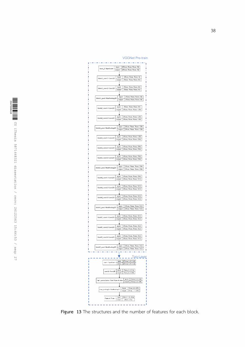
CU iThesis 5871448321 dissertation / recv: 26122563 15:44:53 / seq: 27
38
Figure 13 The structures and the number of features for each block.
VGGNet Pre-train
Top-Layer
25
47
59
94
10
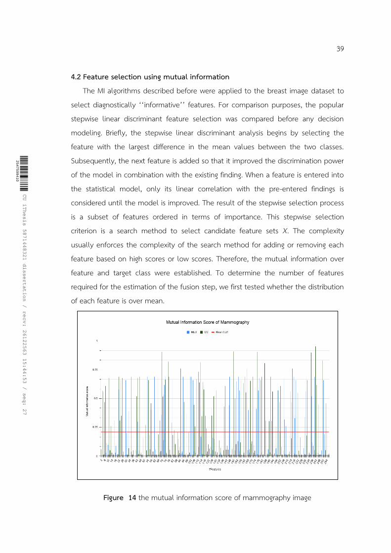
CU iThesis 5871448321 dissertation / recv: 26122563 15:44:53 / seq: 27
39
4.2 Feature selection using mutual information The MI algorithms described before were applied to the breast image dataset to
select diagnostically ‘‘informative’’ features. For comparison purposes, the popular stepwise linear discriminant feature selection was compared before any decision modeling. Briefly, the stepwise linear discriminant analysis begins by selecting the feature with the largest difference in the mean values between the two classes. Subsequently, the next feature is added so that it improved the discrimination power of the model in combination with the existing finding. When a feature is entered into the statistical model, only its linear correlation with the pre-entered findings is considered until the model is improved. The result of the stepwise selection process is a subset of features ordered in terms of importance. This stepwise selection criterion is a search method to select candidate feature sets X. The complexity usually enforces the complexity of the search method for adding or removing each feature based on high scores or low scores. Therefore, the mutual information over feature and target class were established. To determine the number of features required for the estimation of the fusion step, we first tested whether the distribution of each feature is over mean.
Figure 14 the mutual information score of mammography image
25
47
59
94
10

CU iThesis 5871448321 dissertation / recv: 26122563 15:44:53 / seq: 27
40
To explore the features contributing to the target class, we calculated the mutual information of each feature set, and selected the source image for each feature. The distribution of each feature is over mean were selected. The top view (CC) has 87 features, while the side view (MLO) has 75 features.
Figure 15 the mutual information score of ultrasound image
To explore the features contributing to the target class, we calculated the mutual information of each feature set, and selected the source image for each feature. The distribution of each feature is over mean were selected. The B-mode has 78 features, while the Doppler mode has 76 features.
25
47
59
94
10
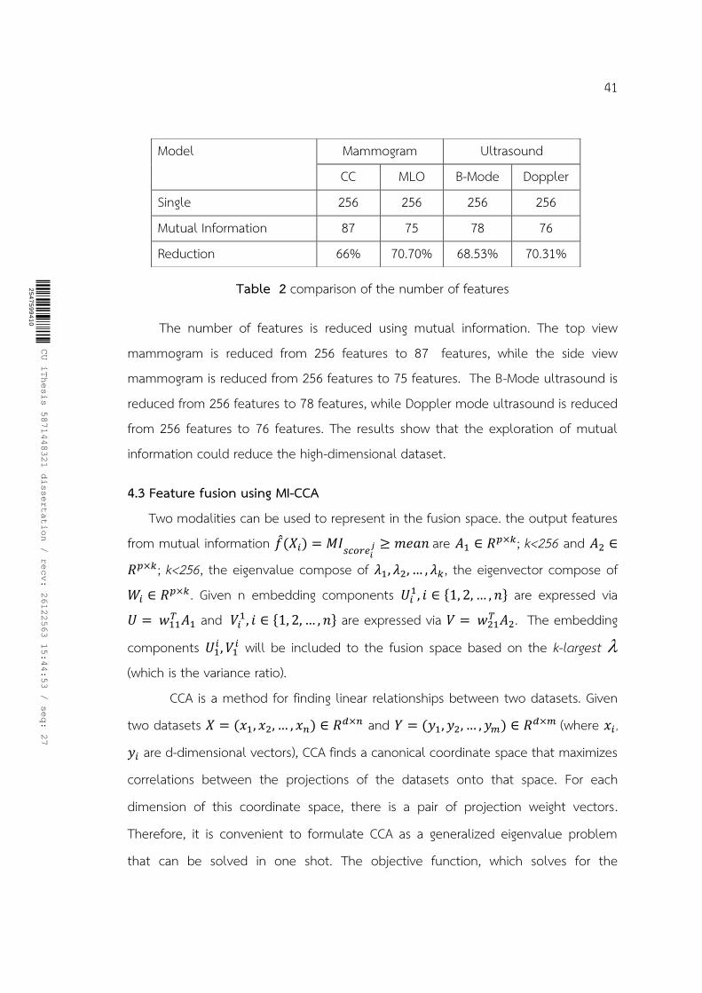
CU iThesis 5871448321 dissertation / recv: 26122563 15:44:53 / seq: 27
41
Table 2 comparison of the number of features
The number of features is reduced using mutual information. The top view mammogram is reduced from 256 features to 87 features, while the side view mammogram is reduced from 256 features to 75 features. The B-Mode ultrasound is reduced from 256 features to 78 features, while Doppler mode ultrasound is reduced from 256 features to 76 features. The results show that the exploration of mutual information could reduce the high-dimensional dataset.
4.3 Feature fusion using MI-CCA Two modalities can be used to represent in the fusion space. the output features
from mutual information 𝑓(𝑋𝑖) = 𝑀𝐼𝑠𝑐𝑜𝑟𝑒𝑖
𝑗 ≥ 𝑚𝑒𝑎𝑛 are 𝐴1 ∈ 𝑅𝑝×𝑘; k<256 and 𝐴2 ∈
𝑅𝑝×𝑘; k<256, the eigenvalue compose of 𝜆1, 𝜆2, … , 𝜆𝑘, the eigenvector compose of 𝑊𝑖 ∈ 𝑅𝑝×𝑘. Given n embedding components 𝑈𝑖
1, 𝑖 ∈ {1, 2, … , 𝑛} are expressed via 𝑈 = 𝑤11
𝑇 𝐴1 and 𝑉𝑖1, 𝑖 ∈ {1, 2, … , 𝑛} are expressed via 𝑉 = 𝑤21
𝑇 𝐴2. The embedding
components 𝑈1𝑖 , 𝑉1
𝑖 will be included to the fusion space based on the k-largest (which is the variance ratio).
CCA is a method for finding linear relationships between two datasets. Given
two datasets 𝑋 = (𝑥1, 𝑥2, … , 𝑥𝑛) ∈ 𝑅𝑑×𝑛 and 𝑌 = (𝑦1, 𝑦2, … , 𝑦𝑚) ∈ 𝑅𝑑×𝑚 (where 𝑥𝑖 ,
𝑦𝑖 are d-dimensional vectors), CCA finds a canonical coordinate space that maximizes
correlations between the projections of the datasets onto that space. For each
dimension of this coordinate space, there is a pair of projection weight vectors.
Therefore, it is convenient to formulate CCA as a generalized eigenvalue problem
that can be solved in one shot. The objective function, which solves for the
Model Mammogram Ultrasound CC MLO B-Mode Doppler
Single 256 256 256 256
Mutual Information 87 75 78 76 Reduction 66% 70.70% 68.53% 70.31%
25
47
59
94
10

CU iThesis 5871448321 dissertation / recv: 26122563 15:44:53 / seq: 27
42
maximum of the canonical correlation vector, is rewritten in terms of the sample
covariance 𝐶𝑥𝑦 of datasets X and Y and the autocovariances 𝐶𝑥𝑥 and 𝐶𝑦𝑦: 𝜌
= maximize𝑤1,𝑤2
𝑤1𝑇𝐶𝑥𝑦𝑤2
√(𝑤1𝑇𝐶𝑥𝑥𝑤1)(𝑤2
𝑇𝐶𝑦𝑦𝑤2)
(4)
Without constraints on the canonical weights 𝑤1 and 𝑤2, the objective
function has infinite solutions. However, the size of the canonical weights can be
constrained, such that 𝑤1𝑇𝐶𝑥𝑥𝑤1 = 1, and 𝑤2
𝑇𝐶𝑦𝑦𝑤2 = 1 This constraint results in the
following Lagrangian:
𝐿(λ, 𝑤1, 𝑤2) = 𝑤1𝑇𝐶𝑥𝑦𝑤2 −
λx
2 (𝑤1
𝑇𝐶𝑥𝑥𝑤1 − 1) −λy
2 (𝑤2
𝑇𝐶𝑦𝑦𝑤2 − 1)
The objective function can then be formulated as the following generalized
eigenvalue problem:
[0 𝐶𝑥𝑦
𝐶𝑦𝑥 0] ∙ [
𝑤1
𝑤2] = 𝜌2 [
𝐶𝑥𝑥 00 𝐶𝑦𝑦
]
The generalized eigenvalue problem is also modified to incorporate
regularization:
[0 𝐶𝑥𝑦
𝐶𝑦𝑥 0] ∙ [
𝑤1
𝑤2] = 𝜌2 [
𝐶𝑥𝑥 + λI 00 𝐶𝑦𝑦 + λI
]
Regularized CCA is mathematically like partial least squares regression (PLS).
Compare to the objective function of CCA (Equation 4) the objective function that is
optimized in PLS:
𝜌 = maximize𝑤1∈𝑅𝑝,𝑤2∈𝑅𝑞
𝑤1𝑇𝐶𝑥𝑦𝑤2
√(𝑤1𝑇𝑤1𝑤2
𝑇𝑤2)
Analogously to CCA, PLS can be solved as a generalized eigenvalue problem:
[0 𝐶𝑥𝑦
𝐶𝑦𝑥 0] ∙ [
𝑤1
𝑤2] = 𝜌2 [𝐼 0
0 𝐼]
25
47
59
94
10

CU iThesis 5871448321 dissertation / recv: 26122563 15:44:53 / seq: 27
43
Once 𝑊𝑥 and 𝑊𝑦 are obtained, the projected new features, called canonical
variables, are computed by 𝑈 = 𝑤1𝑇𝐴1 and 𝑉 = 𝑤2
𝑇𝐴2
Figure 16 the correlation of original CCA, Concatenate-PCA and MI-CCA Figure 16 shows the comparisons of Pearson correlation of original CCA,
Concatenate-PCA and MI-CCA. The original CCA and MI-CCA show very high correlation (Figure 16a, b, c, d), while the PCA is a lower correlation than CCA strategies (Figure 16e, f). Although PCA seems to distinguish the class label better
25
47
59
94
10

CU iThesis 5871448321 dissertation / recv: 26122563 15:44:53 / seq: 27
44
than CCA, they are rarely optimal because they do not take into account the complementarity of groups of features together, something that most supervised algorithms can use very well.
4.4 Classification task Several experiments have been conducted to evaluate the performance and
efficiency of the proposed models. These models were trained on the training data and tested them on the test data. The diagnostic efficiency was analyzed using the Confusion matrix.
4.4.1 Single mammography Table 3 shows the models’ diagnostic efficiency of the mammography
image. Using the SVM classification, the results achieve an accuracy of 90.00% on the top view (CC) and 96.60% on the side view (MLO).
Dataset Accuracy Sensitivity Specificity F1-Score Precision CC-View 0.90 1 0.82 0.88 0.79
MLO-View 0.91 0.85 0.99 0.92 0.99
Table 3 diagnostic efficiency of the mammography image.
Figure 17 show the Confusion matrix of two views were compared. The sensitivity on the top view (CC) is 0.80, the specificity on the top view (CC) is 1. The sensitivity on the side view (MLO) is 0.99, the specificity on the side view (MLO) is 0.82.
Figure 17 the mammography confusion matrix CC (left) and MLO (right).
25
47
59
94
10

CU iThesis 5871448321 dissertation / recv: 26122563 15:44:53 / seq: 27
45
These results show that the side view is more accurate than the top view. However, the top view seems to distinguish the malignant lesions better than the side view. In addition, we found that the side view seems to distinguish the benign lesions better than the top view.
4.4.2 Single ultrasound Table 4.2 shows the models’ diagnostic efficiency of the breast
ultrasound image. Using the SVM classification, the results achieve an accuracy of 93.23% on the B-Mode and 91.73% on the Doppler mode.
Table 4 diagnostic efficiency of the breast ultrasound image.
Confusion matrix of two modes were compared. The sensitivity on the B-Mode is 0.78, the specificity on the B-Mode is 1. The sensitivity on the Doppler mode is 0.75, the specificity on the Doppler mode is 1.
Figure 18 the confusion matrix of B-Mode (left) and Doppler mode (right).
Dataset Accuracy Sensitivity Specificity F1-Score Precision B-Mode 0.93 0.91 1 0.87 0.78
Doppler mode
0.91 1 0.89 0.85 0.74
25
47
59
94
10

CU iThesis 5871448321 dissertation / recv: 26122563 15:44:53 / seq: 27
46
These results demonstrated that B-Mode is more accurate than the Doppler mode (see Figure 18). From the experiment results, it is consistent with our assumption that the multi-evidence could complement the diagnosis information.
4.2 Fusion strategies 4.2.1 The fusion using PCA
The output from feature extraction was represented by 256 features for each view. Then, two datasets were concatenated into one matrix obtained 512 features. This data matrix is the input data set for PCA.
Mammogram: figure 19 illustrates the maximum percentage of total variance only 5 principal components while remaining components account for less than 0 of the total components. Hence, the 75 components were selected (To equal with MI-CCA). Thus, the new data set is of the dimension 600 × 75. This is the new input set for the SVM classification model.
Ultrasound: figure 20 illustrates the maximum percentage of total variance only 10 principal components while remaining components account for less than 0 of the total components. Hence, the 76 components were selected (To equal with MI-CCA). Thus, the new data set is of the dimension 255 × 76. This is the new input set for the SVM classification model.
Table 5 and table 6 show the model performance and comparisons.
4.2.2 The fusion of mammography using CCA Table 5 shows the models’ diagnostic efficiency of fusion
mammography. When compare with the single dataset, MI-CCA improves high diagnostic accuracy. Using the PCA, the result achieves an accuracy of 0.96, while MI-CCA is achieved high diagnostic accuracy of 0.98.
25
47
59
94
10

CU iThesis 5871448321 dissertation / recv: 26122563 15:44:53 / seq: 27
47
Dataset Accuracy Sensitivity Specificity F1-Score Precision
CC-View 0.90 1 0.82 0.88 0.79 MLO-View 0.91 0.85 0.99 0.92 0.99
PCA 0.96 1 0.93 0.96 0.93
MI-CCA 0.98 0.97 1 0.98 1
Table 5 comparison of diagnostic efficiency of mammography.
Confusion matrix of two fusion strategies were compared (Figure 19). The sensitivity on the PCA is 0.93, the specificity on the PCA is 1. The sensitivity on the MI-CCA is 1, the specificity on the MI-CCA is 1. These results show that proposed MI-CCA is more accurate than the PCA approach.
4.2.3 The fusion of ultrasound Table 4.4 shows the models’ diagnostic efficiency of fusion
mammography. When compare with the single dataset, MI-CCA improves high diagnostic accuracy. Using the PCA, the result achieves an accuracy of 0.91, while MI-CCA is achieved high diagnostic accuracy of 0.95.
Table 6 comparison of diagnostic efficiency of ultrasound.
Confusion matrix of two fusion strategies were compared. The sensitivity on the PCA is 0.80, the specificity on the PCA is 0.95. The sensitivity on the MI-CCA is 0.81, the specificity on the MI-CCA is 1. These results show that proposed MI-CCA is more accurate than the PCA approach. Because of MI-CCA is performed using high
Dataset Accuracy Sensitivity Specificity F1-Score Precision
B-Mode 0.93 0.91 1 0.87 0.78 Doppler mode 0.91 1 0.89 0.85 0.74
PCA 0.91 0.89 0.91 0.84 0.80 MI-CCA 0.95 1 0.94 0.92 0.86
25
47
59
94
10

CU iThesis 5871448321 dissertation / recv: 26122563 15:44:53 / seq: 27
48
mutual information between variables and class labels. Therefore, the variables tend to be more compatible with the class labels than other fusion strategies.
Based on our experiments, the fusion strategies could improve diagnosis performance rather than using a single dataset because multi-evidence in medical diagnosis can provide more relevant information.
4.3 Explain variance ratio
Figure 19 Mammogram explain variance ratio
Figure 20 Ultrasound explain variance ratio
25
47
59
94
10

CU iThesis 5871448321 dissertation / recv: 26122563 15:44:53 / seq: 27
49
The Explained Variance Ratio was used to evaluate the usefulness of features and to choose how many features to use in the model. The explained variance ratio is the percentage of the variance of the selected features. In our experiments, selected features from MI-CCA tend to present the highest number of features that can explain the variance compared with concatenate-PCA method.
25
47
59
94
10

CU iThesis 5871448321 dissertation / recv: 26122563 15:44:53 / seq: 27
Chapter V Discussion
In this work, the multi-evidence learning based on feature fusion strategy of multiple views was performed to build breast cancer classification models. The performance of state-of-the-art CNN architectures on the feature extraction was investigated. Furthermore, the supervised feature selection which explores the mutual information was examined for distinguishing the related feature with the class label to reduce the dimension. Finally, information fusion using canonical correlation analysis was performed to combine multi-evidence features. According to our findings, three challenge problems of multiple dataset learning were solved and discussed.
5.1 Consensus principle and complementary principle The consensus principle and complementary principle could be improved the
diagnosis accuracy. The consensus principle aims to maximize the agreement on multiple distinct evidence, while the complementary principle can be employed to comprehensively and accurately describe the data by using the data that may contain some knowledge that other evidences do not have. According to our experiments and results, multi-evidence learning using MI-CCA tends to good consensus and complementary as show in predictions and explanations.
5.1.1 Mammogram dataset Breast mammography is examined by two views including a side view
(MLO) and top view (CC) of the breast. It is possible that some pitfalls presented in the top view (CC), whereas some missed presented in the side view (MLO).
25
47
59
94
10

CU iThesis 5871448321 dissertation / recv: 26122563 15:44:53 / seq: 27
51
Figure 21 the consensus principle of benign lesion (red circle). The top is the original CC view image and its prediction. The bottom is the original MLO view image and its prediction.
25
47
59
94
10

CU iThesis 5871448321 dissertation / recv: 26122563 15:44:53 / seq: 27
52
Figure 21 shows the consensus principle. The single model in the top view decide this image in 73% malignant, while the side view decide this image in 99% benign. The explanation, the likelihood of false positives is expected in the top view because the top view can distinguish the positive class better than the side view as shown in the result (see Figure 17). In addition, it is possible that multiple views can be employed to describe the data comprehensively and accurately.
Figure 22 the complement principle of malignant lesion (red boundary). The top is the original CC view image and its prediction. The bottom is the original MLO view image and its prediction.
25
47
59
94
10
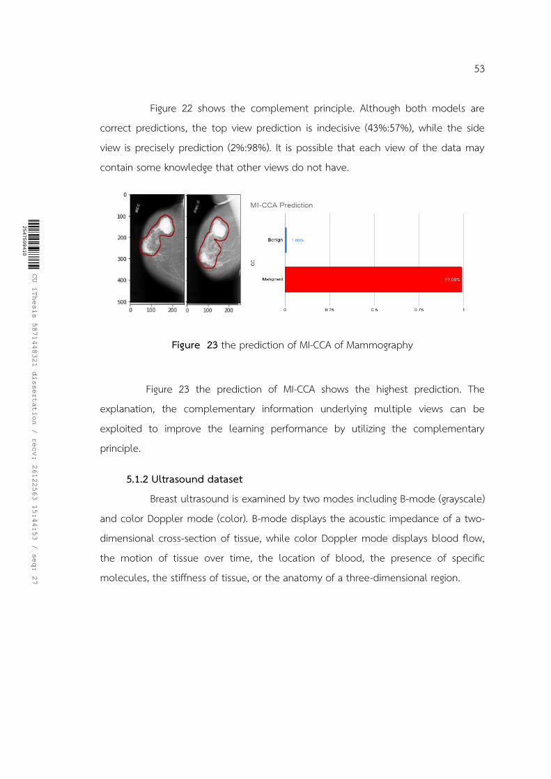
CU iThesis 5871448321 dissertation / recv: 26122563 15:44:53 / seq: 27
53
Figure 22 shows the complement principle. Although both models are correct predictions, the top view prediction is indecisive (43%:57%), while the side view is precisely prediction (2%:98%). It is possible that each view of the data may contain some knowledge that other views do not have.
Figure 23 the prediction of MI-CCA of Mammography
Figure 23 the prediction of MI-CCA shows the highest prediction. The explanation, the complementary information underlying multiple views can be exploited to improve the learning performance by utilizing the complementary principle.
5.1.2 Ultrasound dataset Breast ultrasound is examined by two modes including B-mode (grayscale)
and color Doppler mode (color). B-mode displays the acoustic impedance of a two-dimensional cross-section of tissue, while color Doppler mode displays blood flow, the motion of tissue over time, the location of blood, the presence of specific molecules, the stiffness of tissue, or the anatomy of a three-dimensional region.
25
47
59
94
10

CU iThesis 5871448321 dissertation / recv: 26122563 15:44:53 / seq: 27
54
Figure 24 the consensus principle of malignant lesion. The top is the original B-Mode and its prediction. The bottom is the original Doppler and its prediction.
The single model in B-Mode decide this image in 99% malignant, while the Doppler decide this image in 99% benign.
Figure 25 the prediction of MI-CCA of Ultrasound
Based on the above analysis, ‘MI-CCA’ disseminates the following suggestions: firstly, even if a single evidence approach does not perform well, an ensemble of evidence still can outperform individual evidence. Secondly, since accurate diagnosis is important, models trained on imbalanced training data can
25
47
59
94
10

CU iThesis 5871448321 dissertation / recv: 26122563 15:44:53 / seq: 27
55
provide wrong predictions, due to possible overfitting during the training. In this case, even a high accuracy score can be achieved based on mutual information without predicting minor classes. Thirdly, accurate predictions do not only depend on single imaging modalities but could also build upon additional modalities.
In addition, early detection and diagnosis of breast cancer is critical for survival [62-64]. Early diagnosis requires accurate and reliable tool to distinguish benign and malignant tumors. The major cancer screening problems are false negative to effect with the patients who lose the chance to early treatment. The false positive developed unnecessary surgery such as biopsy. Our experiments reduce the false positive and false negative, furthermore, overall accuracy is better than the single model.
5.2 The correlation among datasets One traditional solution for the multi-view problem is to concatenate vectors
from different views into a new vector and then apply single-view learning algorithms straightforwardly on the concatenated vector. However, different data sources may have correlated and uncorrelated features. Correlation-based techniques have been used to find a set of new attributes that correlate and ensure their compatible between multiple views. Therefore, not only high accuracy but also the maximal correlation has been important. Data fusion as described in Zhang et al [65]. noted that dataset X and Y will be similar information when there is a maximal correlation. When two modalities are maximally correlated, each modality tends to represent similar information. Thus, two objects, which are a high correlation, will be added to the subspace. In practical, the advantage of data fusion should meet two requirements [66]. First, the final layer should be accurate. Second, the fusion layers should be high relationship among views. Our results differ from paper [67] that reported maximized the correlation of dataset.
Three implementations of Original-CCA, PCA, and MI-CCA are compared by Pearson correlation. The proposed MI-CCA not only had the highest correlation but also the mutual information was helpful to maximize the accuracy performance.
25
47
59
94
10
CU iThesis 5871448321 dissertation / recv: 26122563 15:44:53 / seq: 27
56
Moreover, when the prediction relies on investigating the outlier, an MI-CCA may provide the best fit and robust to outliers.
5.3 Dimension reduction of a huge dataset Canonical correlation analysis (CCA) is a multivariate statistical method which
describes the associations between two sets of variables. The objective is to find linear combinations of the variables in each data set having maximal correlation. However, the multiple datasets are typically high-dimensional, containing a lot of variables. In high dimensional setting, the classical canonical correlation analysis is complicated.
We propose a sparse canonical correlation analysis by adding mutual information on the canonical vectors. A two-stage approach to the sparse CCA problems was introduced, where in the first stage we computed the mutual information between the feature and the class labels. Then the distribution of each feature is over mean were selected. These sparsity features shrink smaller matrices and use to the CCA step. Our experiment demonstrated that the mammogram dataset reduced by more than 60%, while the ultrasound dataset reduced by more than 70%. These results show that the search space tends to reduce the boundaries set. Contrary to other popular sparse CCA procedures[68, 69] (i.e. Witten et al., 2009; Parkhomenko et al., 2009) smaller matrices are determined in covariance metrics instead of the high dimension in original CCA. In the other work, Lykou and Whittaker (2010) [70] also treat CCA as a least squares problem. They focus on orthogonality properties of CCA and only construct the first two pairs of sparse canonical vectors. Their approach could be extended to higher order canonical correlations, but this would increase the number of orthogonality constraints and the computing time substantially.
5.4 Summary The applications of the multi evidences learning used in this present study
provide useful insights into the information. The findings can be summarized as follows:
25
47
59
94
10

CU iThesis 5871448321 dissertation / recv: 26122563 15:44:53 / seq: 27
57
• The feature selection criterion can minimize the error rate by considering the mutual information of feature sets. This mutual information is maximized by having a high predictive probability for all the true labels of a training dataset. In general, we can adjust the quality of our training model, but we should not adjust upon the data that will be affected with overfitting problem. Assuming from mutual information allows us to select feature sets which maximizes the high predictive probability, and then to build classification models which maximize the probability based on that feature sets.
• Both complementary and consensus principles play important roles in multi-evidence learning. By considering the complementary information underlying distinct views, advantage can be taken of metric learning to construct a shared latent subspace to precisely measure the dissimilarity between different examples. In other words, the complementary information in distinct views that influences the performance of classification model.
• The strength of correlation between two quantitative variables means that two or more variables have a strong relationship with each other, while a weak correlation means that the variables are hardly related. This conclusion plays important role with data combination strategy. It is very important to understand relationship between variables to draw the right conclusion from a statistical analysis. The relationship between variables determines how the right conclusions are reached. Without high correlation of dataset, many pitfalls can appear that accompany statistical analysis and infer wrong results from fusion data.
25
47
59
94
10

CU iThesis 5871448321 dissertation / recv: 26122563 15:44:53 / seq: 27
Chapter VI Conclusion and Future Work
6.1 Conclusion In this study, we proposed a multi-evidence learning model that utilizes the
extracted information of two views of mammograms and two modes of breast ultrasound for breast cancer classification. We concluded that multi-evidence feature fusion based on mutual information including canonical correlation analysis is more efficient than a single view system. We demonstrated on three challenging. First, MI-CCA plays an important role in consensus and complementary when a single evidence approach has an ambiguous interpretation. Second, correlation-based techniques have been used to find a set of new attributes that correlate and ensure their compatible between multiple views. The proposed MI-CCA not only had the highest correlation but also the mutual information was helpful to maximize the accuracy performance. Finally, dimension reduction of a huge dataset is considered. The mutual information shrinks smaller matrices and use to the CCA. Our experiment demonstrated that the mammogram dataset reduced by more than 60%, while the ultrasound dataset reduced by more than 70%. Additionally, we demonstrated that multi-evidence learning over the mutual information including canonical correlation analysis led to a more refined feature representation that also resulted in increased classification accuracy.
6.2 Limitations of MI-CCA and Future Perspective This study can learn models from multi-evidence data by considering the fusion
of different views. The experimental results show the extensive development of multi-evidence learning and its promising performance compared to single model learning. However, some limitations of our study should be considered.
In theoretical perspective, estimating mutual information from samples struggle to scale up to modern machine learning problems. There are two limitations of variational approaches to MI estimation. The theoretically demonstrate that the
25
47
59
94
10

CU iThesis 5871448321 dissertation / recv: 26122563 15:44:53 / seq: 27
59
variance of certain estimators is high. These limitations challenge the effectiveness of these methods for estimating or optimizing MI.
In diagnosis perspective, First, the other information such as patient demographics and health history were not included. Second, other significant tumor characteristics such as dense breast or fat breast were considered. Finally, more sample datasets were included in future work. In addition, like the clinicians' decision, other medical evidence should be fused for diagnosis.
25
47
59
94
10

CU iThesis 5871448321 dissertation / recv: 26122563 15:44:53 / seq: 27
REFERENCES
REFERENCES
[1] J. Zhao, X. J. Xie, X. Xu, and S. L. Sun, "Multi-view learning overview: Recent progress and new challenges," Information Fusion, vol. 38, pp. 43-54, Nov 2017.
[2] M. L. Sanjoy Dasgupta, David McAllester, "PAC Generalization Bounds for Co-training," Advances in Neural Information Processing Systems 14 (NIPS 2001), vol. 14, pp. 375-382, 2001.
[3] T. Xia, D. Tao, T. Mei, and Y. Zhang, "Multiview Spectral Embedding," Ieee Transactions on Systems Man and Cybernetics Part B-Cybernetics, vol. 40, no. 6, pp. 1438-1446, Dec 2010.
[4] J. Yu, M. Wang, and D. Tao, "Semisupervised Multiview Distance Metric Learning for Cartoon Synthesis," Ieee Transactions on Image Processing, vol. 21, no. 11, pp. 4636-4648, Nov 2012.
[5] C. H. L. Novi Quadrianto, "Learning Multi-View Neighborhood Preserving Projections," Proceedings of the 28th International Conference on Machine Learning, pp. 425-432, 2011.
[6] D. Zhai, H. Chang, S. Shan, X. Chen, and W. Gao, "Multiview Metric Learning with Global Consistency and Local Smoothness," ACM Transactions on Intelligent Systems and Technology, vol. 3, no. 3, pp. 1-22, 2012.
[7] J. Z. Ning Chen, Eric Xing, "Predictive Subspace Learning for Multi-view Data: a Large Margin Approach," Advances in Neural Information Processing Systems 23:
24th Annual Conference on Neural Information Processing Systems, vol. 23, pp. 361-369, 2010.
[8] M. Salzmann, C. H. Ek, R. Urtasun, and T. Darrell, "Factorized Orthogonal Latent Spaces," Journal of Machine Learning Research - Proceedings Track, vol. 9, pp.
701-708, 12/13 2010.
[9] Y. Jia, M. Salzmann, and T. Darrell, Factorized Latent Spaces with Structured Sparsity. 2010, pp. 982-990.
[10] C. Wan, R. Pan, and J. Li, Bi-Weighting Domain Adaptation for Cross-Language Text Classification. 2011, pp. 1535-1540.
25
47
59
94
10

CU iThesis 5871448321 dissertation / recv: 26122563 15:44:53 / seq: 27
61
[11] B. Wei and C. Pal, Cross Lingual Adaptation: An Experiment on Sentiment Classifications. 2010, pp. 258-262.
[12] M.-R. Amini and C. Goutte, "A co-classification approach to learning from multilingual corpora," Machine Learning, vol. 79, no. 1-2, pp. 105-121, May 2010.
[13] H. Hotelling, "Relations Between Two Sets of Variates," Biometrika, vol. 28, pp. 321-377, 11/30 1935.
[14] A. Sharma, A. Kumar, H. Daume, and D. W. Jacobs, Generalized Multiview Analysis: A discriminative latent space. 2012, pp. 2160-2167.
[15] D. Zhai, H. Chang, S. Shan, X. Chen, and W. Gao, "Multiview Metric Learning with Global Consistency and Local Smoothness," ACM Transactions on Intelligent Systems and Technology (TIST), vol. 3, 05/01 2012.
[16] G. Lee et al., "Supervised Multi-View Canonical Correlation Analysis (sMVCCA): Integrating Histologic and Proteomic Features for Predicting Recurrent Prostate Cancer," IEEE Transactions on Medical Imaging, 09/05 2014.
[17] C. Liu and P. C. Yuen, "A Boosted Co-Training Algorithm for Human Action Recognition," Circuits and Systems for Video Technology, IEEE Transactions on, vol. 21, pp. 1203-1213, 10/01 2011.
[18] Y. LeCun, Y. Bengio, and G. Hinton, "Deep Learning," Nature, vol. 521, pp. 436-44, 05/28 2015.
[19] G. V. De La Cruz, Jr., Y. Du, and M. E. Taylor, "Pre-training with non-expert human demonstration for deep reinforcement learning," Knowledge Engineering Review, vol. 34, Jul 26 2019, Art. no. e10.
[20] A. Krizhevsky, I. Sutskever, and G. E. Hinton, "ImageNet Classification with Deep Convolutional Neural Networks," Communications of the Acm, vol. 60, no. 6, pp. 84-90, Jun 2017.
[21] G. Litjens et al., "A survey on deep learning in medical image analysis," Medical Image Analysis, vol. 42, pp. 60-88, Dec 2017.
[22] P. Sermanet, D. Eigen, X. Zhang, M. Mathieu, R. Fergus, and Y. Lecun, "OverFeat: Integrated Recognition, Localization and Detection using Convolutional Networks," International Conference on Learning Representations (ICLR) (Banff), 12/21 2013.
25
47
59
94
10

CU iThesis 5871448321 dissertation / recv: 26122563 15:44:53 / seq: 27
62
[23] A. Singanamalli et al., Supervised Multi-View Canonical Correlation Analysis: Fused Multimodal Prediction of Disease Diagnosis and Prognosis. 2014.
[24] R. L. Birdwell, "Combined Screening With Ultrasound and Mammography vs Mammography Alone in Women at Elevated Risk of Breast Cancer," Yearbook of Diagnostic Radiology, vol. 2009, pp. 43-45, 01/01 2009.
[25] K.-H. Ko et al., "Non-mass-like breast lesions at ultrasonography: Feature analysis and BI-RADS assessment," European Journal of Radiology, vol. 84, 10/23 2014.
[26] H. Zhi et al., "Ultrasound Elastography of Breast Lesions in Chinese Women: A Multicenter Study in China," Clinical breast cancer, vol. 13, 07/03 2013.
[27] S. Parajuly, P. Lan, L. Yan, Y. Gang, and L. Lin, "Breast Elastography: A Hospital-Based Preliminary Study in China," Asian Pacific journal of cancer prevention : APJCP, vol. 11, pp. 809-14, 01/01 2010.
[28] R. Guo, G. Lu, B. Qin, and B. Fei, "Ultrasound Imaging Technologies for Breast Cancer Detection and Management: A Review," Ultrasound in Medicine & Biology, vol. 44, 10/01 2017.
[29] Y. Davoudi, B. Borhani, M. Pezeshki Rad, and N. Matin, "The Role of Doppler Sonography in Distinguishing Malignant from Benign Breast Lesions," Journal of Medical Ultrasound, vol. 22, 06/01 2014.
[30] N. Cho, M. Jang, C. Lyou, J. S. Park, H. Choi, and W. K. Moon, "Distinguishing Benign from Malignant Masses at Breast US: Combined US Elastography and Color Doppler US-Influence on Radiologist Accuracy," Radiology, vol. 262, pp. 80-
90, 11/14 2011.
[31] L. Rocher et al., "Characterization of Testicular Masses in Adults: Performance of Combined Quantitative Shear Wave Elastography and Conventional Ultrasound," Ultrasound in Medicine & Biology, vol. 45, 12/01 2018.
[32] J. Lee, S. Kim, B. Kang, S. Kim, and G. Park, "Evaluation of the effect of computer aided diagnosis system on breast ultrasound for inexperienced radiologists in describing and determining breast lesions," Medical Ultrasonography, vol. 21, 07/05 2019.
[33] S. Roberts-Klein, E. Iuanow, and P. Slanetz, "Avoiding Pitfalls in Mammographic Interpretation," Canadian Association of Radiologists journal = Journal
25
47
59
94
10

CU iThesis 5871448321 dissertation / recv: 26122563 15:44:53 / seq: 27
63
l'Association canadienne des radiologistes, vol. 62, pp. 50-9, 02/01 2011.
[34] L. Bassett et al., "Survey of Radiology Residents: Breast Imaging Training and Attitudes1," Radiology, vol. 227, pp. 862-9, 07/01 2003.
[35] L. Bassett, J. Lubisich, J. Bresch, N. Jessop, and R. E. Hendrick, "Quality assurance in mammography: Status of residency education," AJR. American journal of roentgenology, vol. 160, pp. 271-4, 03/01 1993.
[36] M. Popli, R. Teotia, M. Narang, and H. Krishna, "Breast Positioning during Mammography: Mistakes to be Avoided," Breast cancer : basic and clinical research, vol. 8, pp. 119-24, 07/30 2014.
[37] P. J. Subramanian Maruthathurai Vijayarajan, "Breast Cancer Segmentation and Detection Using MultiView Mammogram," Academic Journal of Cancer Research, vol. 7, pp. 131-140, 2014.
[38] K. Geras, S. Wolfson, S. Kim, L. Moy, and K. Cho, "High-Resolution Breast Cancer Screening with Multi-View Deep Convolutional Neural Networks," 03/21 2017.
[39] L. Sun, J. Wang, Z. Hu, Y. xu, and Z. Cui, "Multi-View Convolutional Neural Networks for Mammographic Image Classification," IEEE Access, vol. PP, pp. 1-1, 09/03 2019.
[40] M. Minsky and S. Papert, Perceptrons: An Introduction to Computational Geometry. 2017.
[41] D. Koller and M. Sahami, "Toward Optimal Feature Selection," Proceedings of the 13th International Conference on Machine Learning (ICML-1996), vol. 96, 10/26 2000.
[42] K. Pearson, "On Lines and Planes of Closest Fit to Points in Space," Philosophical Magazine, vol. 2, pp. 559-572, 11/30 1900.
[43] I. Guyon, S. R. Gunn, M. Nikravesh, and L. Zadeh, "Feature extraction: foundations and applications," 01/01 2006.
[44] M. Bucci, "Optimization with simulated annealing," C/C++ Users Journal, vol. 19, pp. 10-27, 01/01 2001.
[45] H. Peng, F. Long, and C. Ding, "Feature Selection Based On Mutual Information: Criteria of Max-Dependency,Max-Relevance, and Min-Redundancy," IEEE transactions on pattern analysis and machine intelligence, vol. 27, pp. 1226-38,
25
47
59
94
10

CU iThesis 5871448321 dissertation / recv: 26122563 15:44:53 / seq: 27
64
09/01 2005.
[46] P. Somol, P. Pudil, and J. Kittler, "Fast Branch & Bound Algorithms for Optimal Feature Selection," IEEE transactions on pattern analysis and machine intelligence, vol. 26, pp. 900-12, 07/01 2004.
[47] N. Sloane and A. Wyner, "A Mathematical Theory of Communication," pp. 5-83, 11/02 2009.
[48] L. Paninski, "Estimation of Entropy and Mutual Information," Neural Computation, vol. 15, pp. 1191-1253, 06/01 2003.
[49] B. Poczos and J. Schneider, "Nonparametric Estimation of Conditional Information and Divergences," International Conference on AI and Statistics (AISTATS), vol. 20, 01/01 2012.
[50] G. Bontempi and P. Meyer, Causal filter selection in microarray data. 2010, pp. 95-102.
[51] W. Buntine, "Theory Refinement on Bayesian Networks," Proceedings of the 7th Conference on Uncertainty in Artificial Intelligence (UAI-1991), 10/17 1995.
[52] B. Abramson, J. Brown, W. Edwards, A. Murphy, and R. Winkler, "Hailfinder: A Bayesian system for forecasting severe weather," International Journal of Forecasting, vol. 12, pp. 57-71, 02/01 1996.
[53] C. Chih-Chung and L. Chih-Jen, "Libsvm: a library for support vector machines," ACM Trans. Intell. Syst. Technol., vol. 2(3), pp. 1-27, 01/01 2011.
[54] C. Aliferis, A. Statnikov, I. Tsamardinos, S. Mani, and X. Koutsoukos, "Local Causal and Markov Blanket Induction for Causal Discovery and Feature Selection for Classification Part II: Analysis and Extensions," Journal of Machine Learning Research, vol. 11, pp. 235-284, 03/01 2010.
[55] O. Chapelle and S. Keerthi, "Multi-class Feature Selection with Support Vector Machines," American statistical association, 01/01 2008.
[56] Q. Guan et al., "Deep convolutional neural network VGG-16 model for differential diagnosing of papillary thyroid carcinomas in cytological images: a pilot study," J Cancer, vol. 10, no. 20, pp. 4876-4882, 2019.
[57] F. Gao et al., "SD-CNN: A shallow-deep CNN for improved breast cancer diagnosis," Comput Med Imaging Graph, vol. 70, pp. 53-62, Dec 2018.
25
47
59
94
10

CU iThesis 5871448321 dissertation / recv: 26122563 15:44:53 / seq: 27
65
[58] A. Kraskov, H. Stögbauer, and P. Grassberger, "Estimating Mutual Information," Physical review. E, Statistical, nonlinear, and soft matter physics, vol. 69, p. 066138, 07/01 2004.
[59] B. Ross, "Mutual Information between Discrete and Continuous Data Sets," PloS one, vol. 9, p. e87357, 02/19 2014.
[60] L. F. Kozachenko and N. N. Leonenko, "Sample estimate of entropy of a random vector," Problems of Information Transmission, vol. 23, 04/01 1987.
[61] J. Kettenring, "Canonical Analysis of Several Sets of Variables," Biometrika, vol. 58, 12/01 1971.
[62] H. Weedon-Fekjær, P. Romundstad, and L. Vatten, "Weedon-Fekjaer H, Romundstad PR, Vatten LJModern mammography screening and breast cancer mortality: population study. BMJ 348: g3701," BMJ (Clinical research ed.), vol. 348, p. g3701, 06/17 2014.
[63] M. Jacobs et al., "Multiparametric and Multimodality Functional Radiological Imaging for Breast Cancer Diagnosis and Early Treatment Response Assessment," Journal of the National Cancer Institute. Monographs, vol. 2015, pp. 40-6, 05/01
2015.
[64] A. Bleyer, C. Baines, and A. Miller, "Impact of Screening Mammography on Breast Cancer Mortality," International journal of cancer. Journal international du cancer, vol. 138, 11/12 2015.
[65] Y. Zhang, J. Zhang, Z. Pan, and D. Zhang, "Multi-view dimensionality reduction via canonical random correlation analysis," Frontiers of Computer Science, vol. 10, pp. 1-14, 02/26 2016.
[66] J. Zhao, X. Xijiong, X. Xu, and S. Sun, "Multi-view Learning Overview: Recent Progress and New Challenges," Information Fusion, vol. 38, 02/01 2017.
[67] G. Andrew, R. Arora, J. Bilmes, and K. Livescu, Deep Canonical Correlation Analysis. 2013.
[68] D. Witten, R. Tibshirani, and T. Hastie, "A penalized matrix decomposition, with application to sparse principle components and canonical correlation analysis," Biostatistics, pp. 1-20, 01/01 2009.
[69] E. Parkhomenko, D. Tritchler, and J. Beyene, "Sparse Canonical Correlation
25
47
59
94
10

CU iThesis 5871448321 dissertation / recv: 26122563 15:44:53 / seq: 27
66
Analysis with Application to Genomic Data Integration," Statistical applications in genetics and molecular biology, vol. 8, p. Article 1, 02/01 2009.
[70] A. Lykou and J. Whittaker, "Sparse CCA using a Lasso with positivity constraints," Computational Statistics & Data Analysis, vol. 54, pp. 3144-3157, 12/01 2010.
25
47
59
94
10

CU iThesis 5871448321 dissertation / recv: 26122563 15:44:53 / seq: 27
25
47
59
94
10

CU iThesis 5871448321 dissertation / recv: 26122563 15:44:53 / seq: 27
VITA
VITA
NAME นางสาวต้องใจ แย้มผกา
DATE OF BIRTH 24 มิถุนายน 2523
PLACE OF BIRTH กรุงเทพมหานคร
INSTITUTIONS ATTENDED วิทยาศาสตรมหาบัณฑิต (วิทยาศาสตร์คอมพิวเตอร์)
HOME ADDRESS 388/95 ถนนร่มเกล้าซอย 22 แขวงมีนบุรี เขตมีนบุรี กทม. 10510
PUBLICATION 1. An application of process mining for queueing system in health service, 13th International Joint Conference on Computer Science and Software Engineering (JCSSE), 2016 Integrated Dataset Method for Breast Cancer Prediction, International Conference on Innovation in Cancer Research and Care, 18-20 December 2017, Bangkok, Thailand. 2. Combination of B-mode and color Doppler mode using mutual information including canonical correlation analysis for breast cancer diagnosis Medical Ultrasonography, Vol 22, No 1, 2020, p49-57
25
47
59
94
10