multi-constellation gnss scintillation at mid-latitudes ... · multi-constellation gnss...
TRANSCRIPT
Multi-Constellation GNSS Scintillation at Mid-Latitudes
Marc Henri Jean
Thesis submitted to the faculty of the Virginia Polytechnic Institute and State
University in partial fulfillment of the requirements for the degree of
Master of Science
In
Electrical Engineering
Wayne A. Scales
Scott M. Bailey
Dennis G. Sweeney
11/22/2016
Blacksburg, VA
Keywords: Mid-Latitude scintillation, amplitude scintillation, phase scintillation,
Novatel GP6-Station receiver, Novatel Connect, spectral index, histogram
distribution, GPS L1, GPS L2, GPS L5, GLONASS G1, GLONASS G2, Galileo
E1, Galileo E5A, Galileo E5B, SPIRENT GPS Simulator
Multi-Constellation GNSS Scintillation at Mid-Latitudes
Marc Henri Jean
Abstract
Scintillation of Global Positioning Systems (GPS) signals have been extensively studied
at low and high latitude regions of the Earth. It has been shown in past studies that amplitude
scintillation is severe at low latitudes and phase scintillation is severe at high latitudes. Unlike
low and high latitude regions, mid-latitude scintillation has not been extensively studied. Further,
it has been suggested that mid-latitude scintillation is negligible. The purpose of this research is
to challenge this belief.
A multi-constellation and multi-frequency receiver, that tracks American, Russian, and
European satellites, was used to monitor scintillation activity at the Virginia Tech Space Center.
Analysis was performed on collected data from various days and compared to past research done
at high, mid, and low latitudes. The results are discussed in this thesis.
Multi-Constellation GNSS Scintillation at Mid-Latitudes
Marc Henri Jean
General Audience Abstract
Earth’s atmosphere disrupts signals transmitted by Global Navigation Satellite Systems
(GNSS). In certain regions of the Earth, these signals can be severely degraded. Not much
research has been done on what could potentially happen to GNSS signals at mid-latitude regions
of the Earth. It is important to gain a better understanding of the impacts mid-latitude regions can
have on GNSS signals, in preparation for potential future outages across the system.
The United States and Russia have had Global Positioning Systems (GPS) technology for
decades. Today, China and Europe are expanding their global positioning systems. In the future
there may be up to one hundred or more satellites available for public usage. This study was
done to determine if outages could potentially occur at mid-latitudes, and to gain more
knowledge on which of these satellite constellations have the best service.

iv
Acknowledgements
I would like to thank Dr. Wayne Scales for providing his support and wisdom. I would
also like to thank my lab mates Augustine Yellu and Yuxiang (Phillip) Peng for giving me good
advice. Finally, I would like to thank James Conroy for giving me tips on how to code MATLAB
more effectively.
v
Dedication
I would like to dedicate my research to my sisters Lody, Paola, and my grandmother
Jeannette Jean for their support.
vi
Table of Contents
Abstract…………………………………………………………....................................................2
General Audience Abstract………………………………………………………………………..3
Acknowledgments………………………………………………………………………………..iv
Dedication………………………………………………………………………………................v
Table of Contents…………………………………………………………………………………vi
List of Figures…………………………………………………………………………...............viii
List of Tables…………………………………………………………………………………….xii
Chapter 1: Introduction…………………………………………………………………................1
Chapter 2: Technical Background.……...………………………………………………...............4
2.1 GNSS Basics ………………………………………………………………………….4
2.2 Basics of GNSS signal propagation in the Ionosphere………………………………..7
2.3 Basic concept of GNSS scintillation………………………………...……………….12
2.4 Past Scintillation Investigations……………………………………….......................17
2.4.1 Low Latitudes……………………………………...................................................17
2.4.2 High Latitudes…………………………………………………………...................19
2.4.3 Mid Latitudes……………………………………………………………................20
2.4.4 Summary…………………………………………………………………………...21
Chapter 3: Experimental Approach……………………………………………………...............21
3.1 GNSS Receiver……………………………………………………………………....21
3.2 High Rate and Low Rate File Format………………………………………………..24
3.3 Software Design……………………………………………………..........................25
Chapter 4: Experimental Results………………………………………………………...............27

vii
4.1 Introduction…………………………………………………………………………..27
4.2 Data Set 1 Presentation………………………………………………..……………..28
4.2.1 Scintillation Analysis…………………………………………………....…………29
4.2.2 Summary…………………………..…………………………………….................41
4.3 Data Set 2 Presentation…………………………………………………....................45
4.3.1 Scintillation Analysis…..………………………………………………..................46
4.3.2 Summary…………………………………………………………………...............60
4.4 Data Set 3 Presentation…………………………………………................................64
4.4.1 Scintillation Analysis…..………………………………………………..………....65
4.4.2 Statistical and Cross Correlation Analysis…….......……………………………….68
4.4.3 Summary…………………………………………………………………...............81
Chapter 5: GNSS Hardware Signal Simulation of Scintillations Effects………………………..83
Chapter 6: Conclusion and Future Work………………………………………………………...87
References……………………………………………………………………………………….91
Appendix………………………………………………………………………………...............95
Appendix A: Coding Methods………………………………......................................................95
viii
List of Figures
Figure 1: SuperDARN plots of TEC and radar back scatter of storm which occurred on February,
16th 2016 [7] …………………………………………………………………………………........3
Figure 2: Control, space, and user segments of a GPS system [14] ……………………...............6
Figure 3: Ionospheric D, E, and F layers during the day and night time hours. This plot presents
the electron density of each of layer vs. altitude [15] ……………………….................................8
Figure 4: Lower RF reflecting from the ionosphere and high RF penetrating the ionosphere [17]
………………………………………………………………………..............................................9
Figure 5: Power spectral density of phase. Linear fit curves are drawn in the power region
between the low cut off region and high cut off region over desired frequency range f. The
spectral index p is approximated from the linear fit [1]………………………………………….15
Figure 6: Scintillation data collected in Brazil at Cachoeira Paulista, Brazil [20]……................17
Figure 7: Histogram distribution of scintillation of L1 and L2 bands collected using Septentrio
PolaRxS Pro (top) and histogram distribution of scintillation L1 and L5 collected using Novatel
GPStation-6 (bottom) [21]………………………………….........................................................18
Figure 8: Power spectral density of amplitude and phase scintillation, green representing phase
and blue representing amplitude. Both data sets were collected at Lonyearbyen, Norway
[1]…………………………………………………………………………………………..…….19
Figure 9: Linear interpolation of spectral index p over time. As shown on the plot above, p can
vary from values less than 1 to values as high as 3.5 [1]…………………………………..…….20
Figure 10: Power spectral density plot of amplitude generated from data collected at mid-latitude
[2]………………………………………………………………………………………….……..20
Figure 11: Current GP-6 station used at the Virginia Tech GPS lab [23]……………………….22
Figure 12: Novatel connect window, which displays user position, carrier to noise ratio, satellite
elevation and azimuth plot, etc. [24]…………………………………………………………... .23
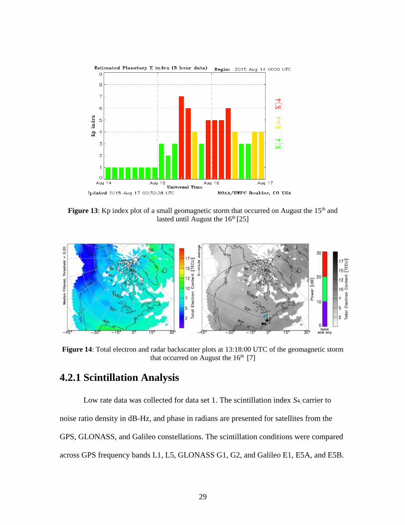
Figure 13: Kp index plot of a small geomagnetic storm that occurred on August the 15th and
lasted until August the 16th [25]…………………………………………………………………29
Figure 14: Total electron and radar backscatter plots at 13:18:00 UTC of the geomagnetic storm
that occurred on August the 16th [7]……………………………………………………………29

ix
Figure 15: Elevation and azimuth plot of satellites analyzed during a turbulent event. The
satellites are represented, by red stars. GPS satellites 9, 27, GLONASS 14, 17, and Galileo 19 are
shown on the plots [26]…………………………………………………………………………..30
Figure 16: Scintillation, carrier to noise ratio, and phase of GPS satellite PRN number 9, at
frequency L1……………………………………………………………………………………..33
Figure 17: Scintillation, carrier to noise ratio, and phase of GPS satellite PRN number 27, at
frequency L1……………………………………………………………………………………..34
Figure 18: Scintillation, carrier to noise ratio, and phase of GPS satellite PRN number 27, at
frequency L5………………………………………………………………………………...…...35
Figure 19: Scintillation, carrier to noise ratio, and phase of GLONASS satellite PRN number 14,
at frequency G1………………………………………………………………………………......36
Figure 20: Scintillation, carrier to noise ratio, and phase of GLONASS satellite PRN number 17,
at frequency G2……………………………………………………………..................................37
Figure 21: Scintillation, carrier to noise ratio, and phase of Galileo satellite PRN number 19, at
frequency E1……………………………………………………………………..........................38
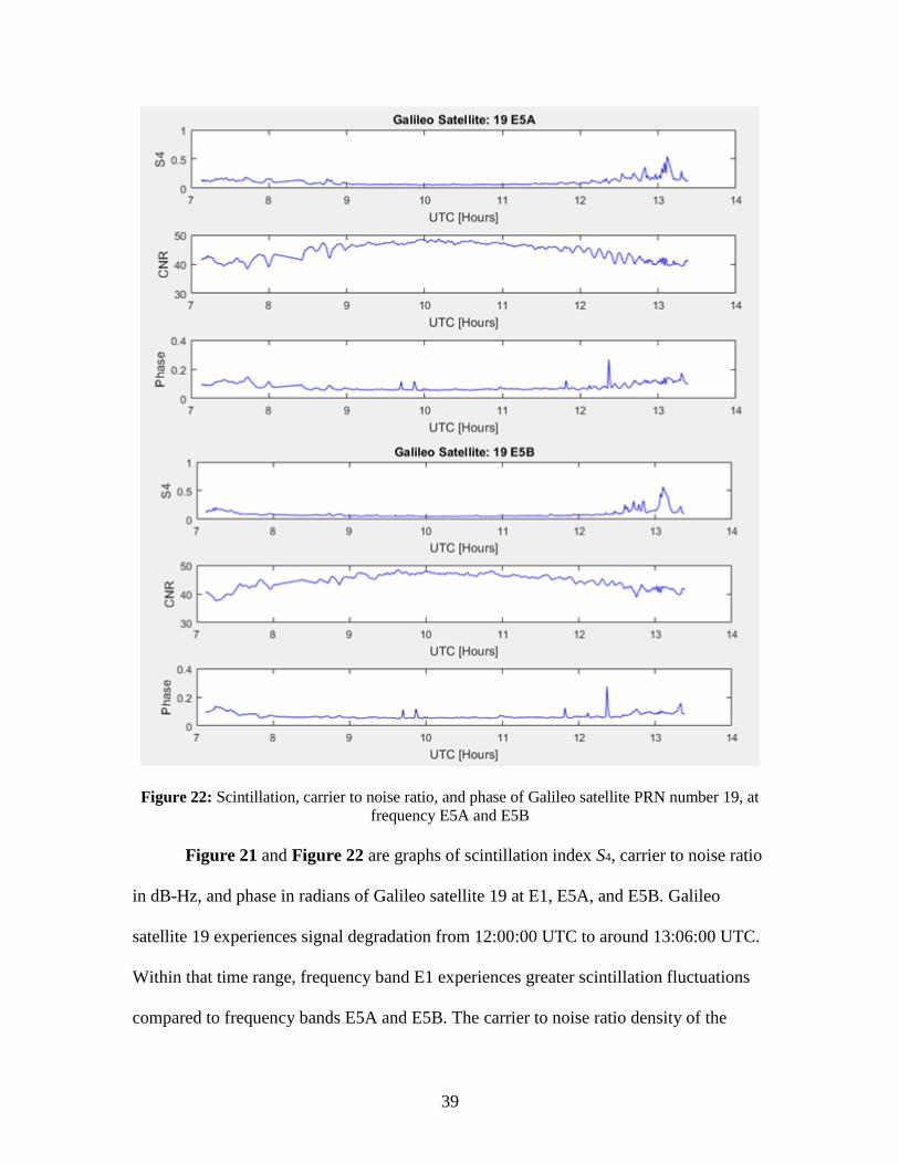
Figure 22: Scintillation, carrier to noise ratio, and phase of Galileo satellite PRN number 19, at
frequency E5A and E5B………………………………………………………..………………..39
Figure 23: Histogram distribution of GPS satellite PRN 9 (L1, L5) and GPS satellite PRN 27
(L1, L5) scintillation above 15 degrees elevation angle…………………………........................41
Figure 24: Histogram distribution of GLONASS satellite (G1, G2) and GLONASS satellite 27
(G1, G2) scintillation above 15 degrees elevation angle…………………………………………43
Figure 25: Histogram distribution of Galileo satellite 19 (E1, E5A, E5B) scintillation above 15
degrees elevation angle……………………………………………………………......................44
Figure 26: Kp index plot of a small geomagnetic storm that occurred on February the 16th and
lasted until February the 17th [25]………………………………………………………………...45
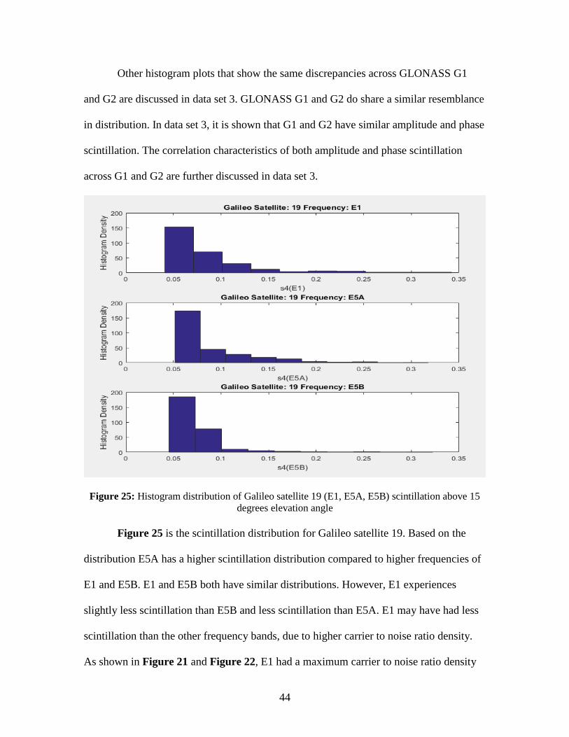
Figure 27: Total electron and radar backscatter plots at 12:00:00 UTC of the geomagnetic storm
that occurred on February the 16th [5]………………………………………..…………………..46
Figure 28: Location of GPS satellite 9 and 24 during the storm on February the 16th [26]
……………………………………………………………………………………………………46
Figure 29: Signal power in dB for GPS satellites 1, 3, 8, 9, 24, 25, 26, 27, L1(red), L2(black),
L5(blue)…………………………………………………………………………………………..49

x
Figure 30: Power spectral density graph amplitude in (blue) for frequency L1, L2C, L5
…………………………………………………………………………………………................52
Figure 31: Signal power in dB for GLONASS satellites 1, 2, 3, and 4 G1 (Red) and G2
(Black)……………………………………………………………………………………………53
Figure 32: Power spectral density graph of amplitude in (blue) for frequency band G1 and
G2………………………………………………………………………………………………...56
Figure 33: Signal strength in dB for Galileo satellite 11, E1 (Red), E5A (Black), and E5B
………………………………………………………………………………………..…………..57
Figure 34: Power spectral density graph of amplitude in (blue) for frequency bands E1, E5A, and
E5B……………………………………………………………………………………................58
Figure 35: High rate amplitude scintillation data for GPS satellite 9 and 24 at L1, L2C, and L5. Abrupt
scintillation occurs at 48 minutes for GPS satellite 9 and 53 minutes for satellite
24…………….…………………………………………………………………………...............61
Figure 36: Power spectral density graph of amplitude in (blue) and phase in (orange) of GPS
satellites 9 and 24………………………………………………………………...........................62
Figure 37: Power spectral index p for GPS satellite 9 over 60 minutes……...……….................63
Figure 38: Range of Kp index values for data set 3, which range from Kp of 2 to 4
[25]….............................................................................................................................................64
Figure 39: Histogram distribution of GPS satellites 26 (top) and 30 (bottom) L1, L2, L5 over 11-
day period……………………………....……………………………..……….............................65
Figure 40: 11-day period and histogram distribution of GPS satellites 6 and 8 (top) and 9 and 27
(bottom) L1, L2, L5 over 11-day period…………………………………...…………………….66
Figure 41: Histogram distributions for GLONASS satellites 2 and 3 G1, G2 over 11-day period
…………………………………….........……………………………...…………………………67
Figure 42: Histogram distributions for Galileo satellites 11 and 12 (top) and Galileo 24 and 26
(bottom) E1, E5A, and E5B over 11-day period...........................................................................68
Figure 43: Statistical analysis done at equatorial and high latitude regions [29]…......................69
Figure 44: Probability distribution of amplitude and phase scintillation across GPS L1, L2, L5 at
mid-latitude for 11 – day period…………………………………………………………………70
Figure 45: Probability distribution of amplitude and phase scintillation across GLONASS G1 and
G2 at mid-latitude for 11 – day period………………...………………………………………...71
xi
Figure 46: Probability of distribution of amplitude and phase scintillation across E1, E5A, E5B at
mid-latitude for 11 – day period………………………………………........................................72
Figure 47: Linear fit curves across GPS L1, L2, L5 amplitude and phase scintillation for satellites
1 and 25 [29]………………………………………………....................……..............................74
Figure 48: Linear fit curves across GPS L1, L2, L5 amplitude and phase scintillation for satellites
1 and 25 [29]…………………………………………………………………..............................77
Figure 49: Linear fit curves across GLONASS amplitude and phase scintillation for satellites 2
and 3…………………………………………………………...………...……………………….78
Figure 50: Linear fit curves across Galileo E1, E5A, E5B amplitude and phase scintillation for
satellites 24 and 26…………………………………………………….........................................81
Figure 51: Virtual scintillation window for SPIRENT GPS simulator. As shown in the figure, a
scintillation value of 0.50 is inputted from 0 degrees latitude to 70 degrees
latitude…………………………………………………………………………………………....84
Figure 52: Ground track window from GPS simulator. The white triangle is the stationary vehicle
placed in Blacksburg, VA. X marks are GPS satellites that are built in virtually in the GPS
simulator ……………………………………………………………....…………………………85
Figure 53: Simulation results for GPS satellite 7 and 20 for frequency bands L1, L2, L5
…………………………………………………………………………………………………....86
xii
List of Tables
Table 1: The figure above is an example of the low rate .CSV file and the columns of data that
are included in it………………………………………………………………………………….24
Table 2: An example of the high rate .CSV file and the columns of data that are included in
it…………………………………………………………………………………….....................25
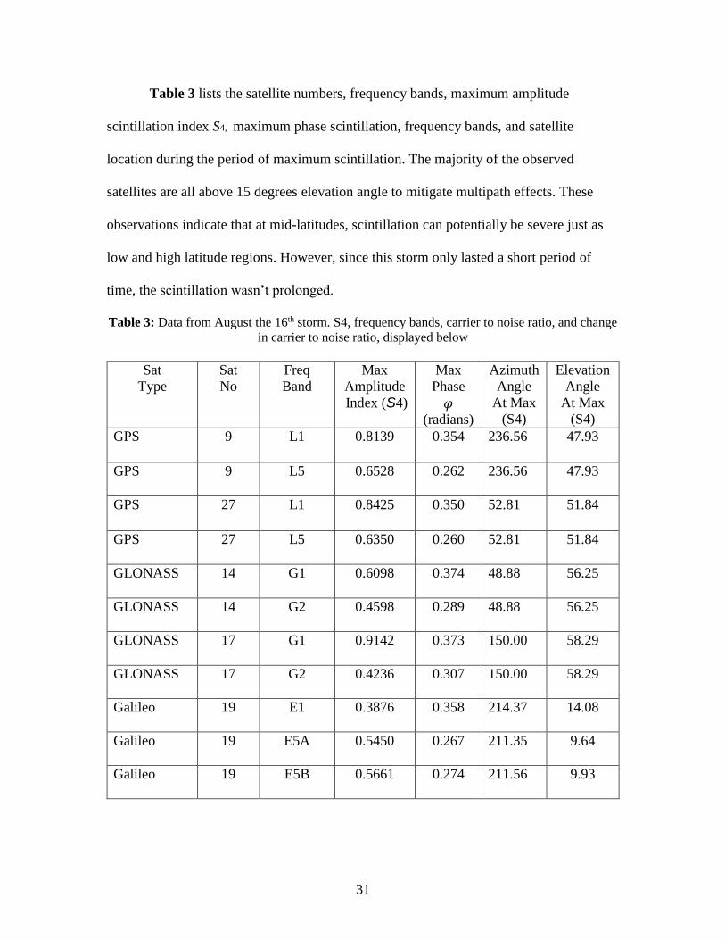
Table 3: Data from August the 16th storm. S4, frequency bands, carrier to noise ratio, and change
in carrier to noise ratio, displayed below………………………………………………………...31
Table 4: GPS Satellite Numbers 1, 3, 8, 9, Frequency Bands, Fresnel Frequency (Ff), and
Spectral Index p…………………………………………………………………………………...............50
Table 5: GPS Satellite Numbers 24, 25, 26, 27, Frequency Bands, Fresnel Frequency (Ff), and
Spectral Index p…………………………………………………………………………………………….51
Table 6: GLONASS Satellite Numbers 1, 2, 3, 4, 6, 8, 10 Frequency Bands, Fresnel Frequency
(Ff), and Spectral Index p………………………………………………………....................................54
Table 7: Galileo Satellite Numbers 11, 12, 22, 24 Frequency Bands, Fresnel Frequency (Ff), and
Spectral Index p …………………………………………………………………………………………59
1
Chapter 1
Introduction
The purpose of this study is to analyze ionospheric scintillation on Global
Navigation Systems (GNSS) signals at mid-latitudes in the northern hemisphere, which
are regions that are between 30 degrees to 60 degrees latitude. It has been shown from
previous studies, which were done at high and low latitudes, that ionospheric turbulence
disrupts GNSS signals, which operate in the L band frequency range [1]. The goal of this
study is to compare scintillation characteristics at mid-latitudes to previous studies done
at high latitudes, which are regions typically between 60 degrees to 90 degrees latitude in
the northern hemisphere and at low latitudes, which are regions typically between 0
degrees latitude to 30 degrees latitude in the northern hemisphere. The corresponding
definitions of latitudinal regions hold true in the southern hemisphere as well.
Scintillation at mid-latitude regions has been considered to be negligible in the
past, compared to high and low latitude regions. According to [1, p1] “In mid-latitude
regions, both amplitude and phase scintillation are negligible”. It can certainly be argued
that scintillations at mid-latitudes should be much weaker than at high and low latitudes.
However, few studies have been done on scintillation at mid-latitude regions and part of
this study is to challenge the belief that mid-latitude scintillation effects are unimportant.
New space science measurement facilities have shown that the physics of
ionospheric irregularities are much more complex than have been thought in the past [2].
Both the Global Navigation Satellite System (GNSS) and SuperDARN space weather
high frequency (HF) radar facilities are used in this study to investigate scintillation at
mid-latitude. A multi-constellation and multi-frequency GNSS receiver, which tracks

2
GPS frequency bands L1 (1.575 GHz), L2 (1.227 GHz), and L5 (1.176 GHz),
GLONASS frequency bands G1 (1.5980625 – 1.6093125) and G2 (1.2429375 –
1.2516875 GHz), and Galileo frequency bands E1 (1.575), E5A (1.176 GHz), and E5B
(1.207 GHz), was used to monitor scintillation activity [3], [4], [5]. This is one of the first
studies of its kind.
SuperDARN radar data were used to observe and further interpret Ionospheric
conditions. SuperDARN collects data using a chain of high frequency (HF) radars to
monitor ionospheric conditions at high and mid latitudes [2]. The chain of radars has 16
to 24 beams that scan at rate of 1 to 2 minutes. SuperDARN radars are pulse radars that
transmit pulses that have a length of 300 microseconds. The radars measure back scatter
from ionospheric structure in the E and F regions, typically resulting from plasma
irregularities [2], [6]. The SuperDARN radar ionosphere scatter plots provide the signal
to noise (SNR) in decibels (dB), which is the ratio of power caused by the back scatter
from the ionosphere and noise power interference.
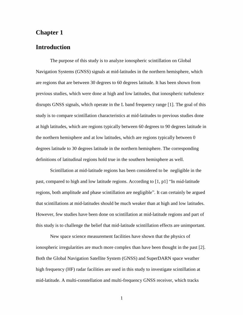
Figure 1 shows the Total Electron Content TEC (left) and SNR from the back
scatter of the of the ionosphere (right). The data was collected during a geomagnetic
storm on February 16th, 2016. The TEC shows levels of electron content as high as 10
total electron content units (TECU) and the back scatter plot shows a signal to noise ratio
(SNR) ranging from 10 to 20 dB in mid-latitude regions above North America. The TEC
and backscatter are used to interpret the ionospheric conditions during the time the
scintillation data is collected. The TEC and backscatter characterize ionospheric
disturbances that produce GNSS scintillation.
3
Figure 1: SuperDARN plots of TEC and radar back scatter of storm which occurred on
February, 16th 2016 [7]
The study of mid-latitude scintillation is very important because not much is
known about how these regions of ionospheric disturbances can affect GNSS signals. For
example, research done in low latitude regions near the equator show that GNSS signals
can be faded during large ionospheric disturbances. However, few detailed investigations
of what could potentially happen to GNSS signals, under the same circumstances at mid-
latitudes, have been undertaken. Since a large percentage of the earth’s population live in
mid-latitude regions of the Earth and are dependent on GNSS technology, it is important
to be prepared for potential GNSS blackouts that may be caused by a severe space
weather event.
Objective of this Study
This research focuses on analyzing the effects that scintillation may have on the
different frequency bands on GPS, Galileo, and GLONASS satellite systems. The
frequency bands analyzed in this research include GPS L1, L2, L5, GLONASS G1, G2,
and Galileo E1, E5A, E5B. These frequency bands are compared to determine which is
degraded less and has the best overall performance relative to mid-latitude scintillations.
The results are compared to previous research done at low latitudes and high latitudes.
Another goal of this research is to analyze the power spectral density of both phase and

4
amplitude scintillation at mid-latitudes. The results are also compared to previous
research done at mid-latitudes and high latitudes. Such studies may ultimately provide
insight into the ionospheric plasma processes causing the turbulence [8]. Finally, the last
part of this research involves simulating scintillation models using a radio frequency (RF)
hardware GPS simulator. The GPS hardware simulator has a built-in virtual scintillation
model, which may allow useful comparisons to the data. The purpose of this study is to
see if mid-latitude scintillation conditions can be replicated using the hardware
simulations across GPS frequency bands L1, L2, and L5.
Chapter 2 Technical Background
2.1 GNSS basics
Global Navigation Satellite Systems (GNSS) are widely used for civilian,
military, and scientific applications. The United States (US) has a total of thirty-two
Global Positioning System (GPS) satellites in its constellation [9]. A minimum of twenty-
four of the satellites are needed for global tracking, with four satellites in six orbital
planes [9]. Aside from the United States, Russia, China, and the European Union (EU)
have operable GNSS constellations. The Russian GLONASS constellation has 24 active
satellites [4]. The Chinese Beidou Constellation has 21 satellites in orbit, and the EU
Galileo constellation currently has 12 satellites [10], [11], [12]. Unlike the other three
GNSS constellations, Galileo is still in early stages of development and is expected to be
completed by 2020 [5]. In the near future, Galileo will have a full fleet of 30 satellites
and Beidou will have 35 [10], [11]. The US GPS satellites have near circular orbits,
which means that the eccentricity of these satellites is nearly zero [9]. The satellites are
located roughly 26,000 km from the center of the Earth, at 55 degree inclinations [9]. By

5
the time all the GNSS constellations are complete, there may be up to 121 available
GNSS satellites available for civilian usage. Having a GNSS receiver will allow users to
track multiple constellations across multiple frequency bands, which will improve
position accuracy and receiver performance.
GNSS transmit signals in the L band range from 1 to 2 GHz. In the L band
frequency range, wavelengths can measure anywhere from 20 cm to 30 cm in length. For
example, GPS satellites transmit wavelengths anywhere from 19 cm to 25 cm. Each of
these constellations have frequency bands that are available for civilian usage. GPS has
three frequency bands, L1, L2, and L5, that are available for civilian usage [3].
GLONASS has two frequency bands available for civilian usage: G1 and G2 [4]. Galileo
has three frequency bands available for civilian usage: E1, E5A, and E5B [5].
GNSS also have different multiple accessing schemes. GPS and Galileo use code
division multiple accessing (CDMA) [3], [5]. In CDMA systems, the same frequency
bands are transmitted across all users, but satellites are identified by pseudo random
codes [13]. Each of the satellites are identified by a unique code. Unlike GPS and
Galileo, GLONASS uses frequency division multiple accessing scheme (FDMA) [4]. In
an FDMA system, frequency is divided within the available spectrum. As a result, each
of the GLONASS satellites in view of a receiver has to transmit a different frequency
band to avoid interference. The 24 GLONASS satellites use a range of 12 different
frequencies. GLONASS satellites can transmit the same frequency for different users
only if the receivers are located 180 degrees apart to avoid interference.
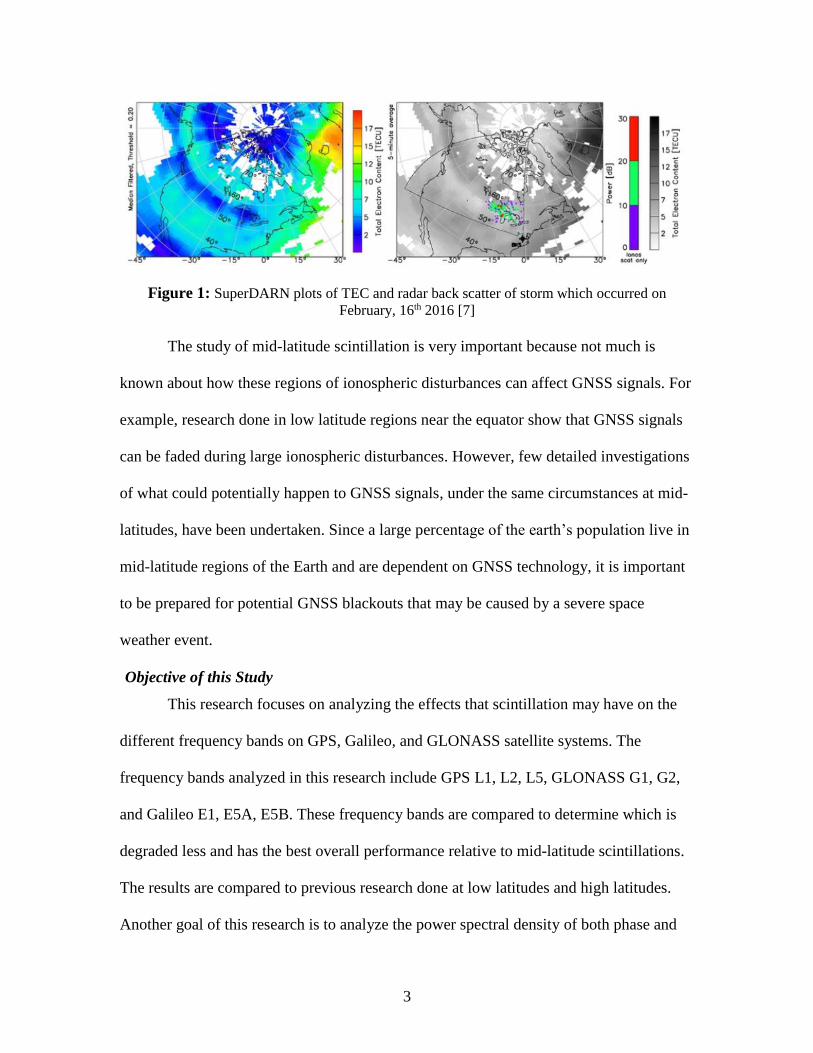
GPS have three important segments shown in Figure 2. The segments include the
control segment, the space segment, and the user segment [9]. The control segment
6
monitors the location of the GPS satellites from Earth. Once the control segment
determines the location of the satellites, it transmits parameters referred to as the
ephemeris, used for determination of the satellite position, back to the GPS satellites in
space, which in turn then transmit the ephemerides to the user segment. The user segment
includes the GPS receivers monitoring the satellites. The ephemerides are used by the
user segment to determine the satellite locations, which are ultimately used in the
navigation solution.
Figure 2: Control, space, and user segments of a GPS system [14]
In order to determine the navigation solution, the user segment needs to be locked
into at least four GPS satellites [9]. Three satellites are needed to determine the unknown
values of X, Y, Z of the user position. The fourth satellite is used to determine the GPS
receiver clock offset. Since there are four unknown variables, four equations are required
to solve the system of four unknown values. Tracking more than four satellites provides a
more accurate solution.
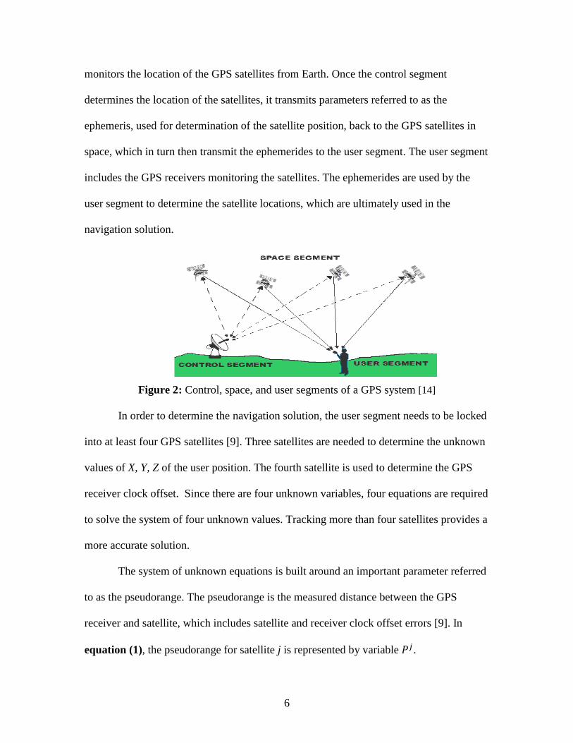
The system of unknown equations is built around an important parameter referred
to as the pseudorange. The pseudorange is the measured distance between the GPS
receiver and satellite, which includes satellite and receiver clock offset errors [9]. In
equation (1), the pseudorange for satellite j is represented by variable 𝑃𝑗 .
7
𝑃𝑗 = 𝜌𝑗 + 𝑐𝛿𝑗 − 𝑐𝛿R (𝟏)
The actual distance from the GPS receiver to the satellite, the range, is represented by
variable 𝜌𝑗. From equation (1) it is seen that the pseuodrange is equal to the actual range
added to the satellite and receiver clock offsets, 𝛿𝑗and 𝛿R, which are multiplied by the
speed of light c.
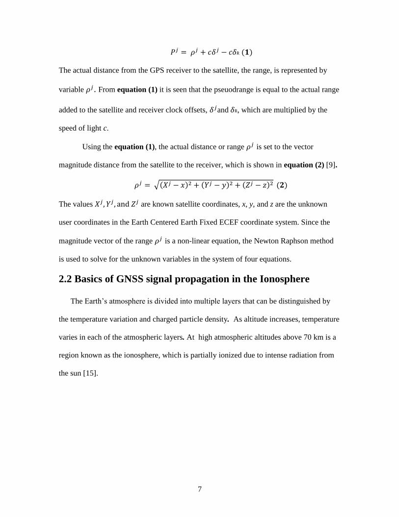
Using the equation (1), the actual distance or range 𝜌𝑗 is set to the vector
magnitude distance from the satellite to the receiver, which is shown in equation (2) [9].
𝜌𝑗 = √(𝑋𝑗 − 𝑥)2 + (𝑌𝑗 − 𝑦)2 + (𝑍𝑗 − 𝑧)2 (𝟐)
The values 𝑋𝑗 , 𝑌𝑗 , and 𝑍𝑗 are known satellite coordinates, x, y, and z are the unknown
user coordinates in the Earth Centered Earth Fixed ECEF coordinate system. Since the
magnitude vector of the range 𝜌𝑗 is a non-linear equation, the Newton Raphson method
is used to solve for the unknown variables in the system of four equations.
2.2 Basics of GNSS signal propagation in the Ionosphere
The Earth’s atmosphere is divided into multiple layers that can be distinguished by
the temperature variation and charged particle density. As altitude increases, temperature
varies in each of the atmospheric layers. At high atmospheric altitudes above 70 km is a
region known as the ionosphere, which is partially ionized due to intense radiation from
the sun [15].
8
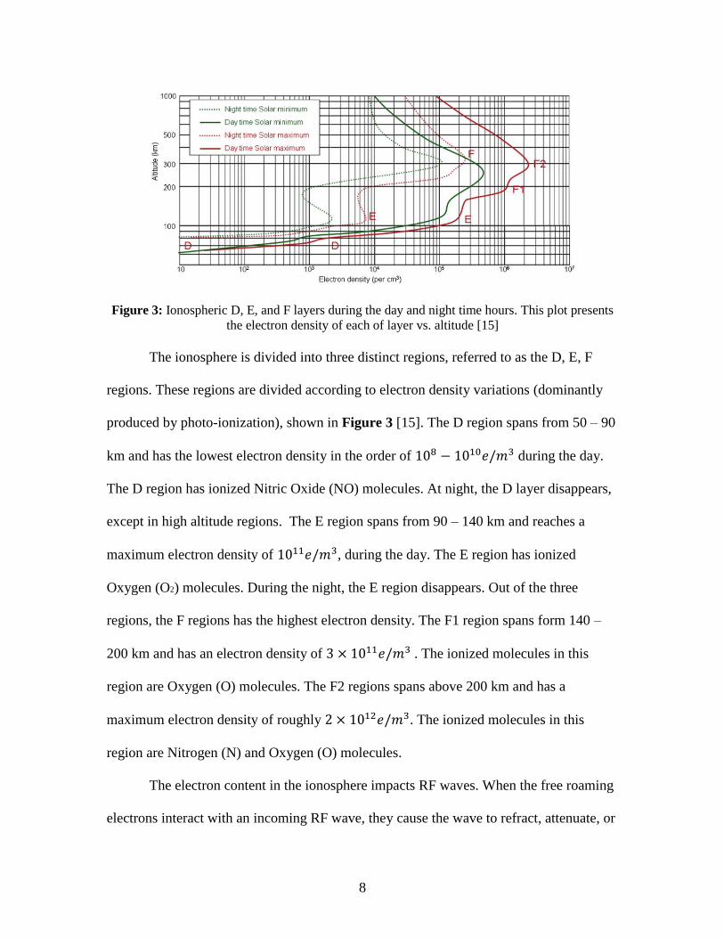
Figure 3: Ionospheric D, E, and F layers during the day and night time hours. This plot presents
the electron density of each of layer vs. altitude [15]
The ionosphere is divided into three distinct regions, referred to as the D, E, F
regions. These regions are divided according to electron density variations (dominantly
produced by photo-ionization), shown in Figure 3 [15]. The D region spans from 50 – 90
km and has the lowest electron density in the order of 108 − 1010𝑒/𝑚3 during the day.
The D region has ionized Nitric Oxide (NO) molecules. At night, the D layer disappears,
except in high altitude regions. The E region spans from 90 – 140 km and reaches a
maximum electron density of 1011𝑒/𝑚3, during the day. The E region has ionized
Oxygen (O2) molecules. During the night, the E region disappears. Out of the three
regions, the F regions has the highest electron density. The F1 region spans form 140 –
200 km and has an electron density of 3 × 10¹¹𝑒/𝑚3 . The ionized molecules in this
region are Oxygen (O) molecules. The F2 regions spans above 200 km and has a
maximum electron density of roughly 2 × 10¹²𝑒/𝑚3. The ionized molecules in this
region are Nitrogen (N) and Oxygen (O) molecules.
The electron content in the ionosphere impacts RF waves. When the free roaming
electrons interact with an incoming RF wave, they cause the wave to refract, attenuate, or

9
disperse [16]. RF waves that operate at frequencies above roughly 10 MHz can penetrate
and travel through the electron density present in the ionosphere [9]. That is, the RF
frequency must be larger than the so-called ionospheric plasma frequency defined as 𝑓𝑝 =
8.98√𝑁𝑒 , which varies based on electron density 𝑁𝑒. RF waves that operate roughly
below the plasma frequency will reflect or refract from the ionosphere. Figure 4 presents
a visual of how waves may reflect and penetrate the ionospheric layer.
Figure 4: Lower RF reflecting from the ionosphere and higher RF penetrating the ionosphere
[17]
Since GNSS satellites operate well above the plasma frequency, they are able to
penetrate and travel through the ionosphere [9]. However, the phase velocity 𝑉𝑝ℎ of the
waves traveling at L band frequency ranges is reduced due to the impact of the electron
density on the refractive index. The index of refraction is described with respect to speed
of light C and phase velocity Vph in equation (3) [18].
𝑛𝒑𝒉 = 𝐶𝑉𝒑𝒉
(𝟑)
Substituting the expression of phase velocity Vph presented in equation (4) into
the denominator of equation(3) gives
10
𝑉𝒑𝒉 =𝑐
√1 − (𝑓𝑝𝑓
)2
(𝟒)
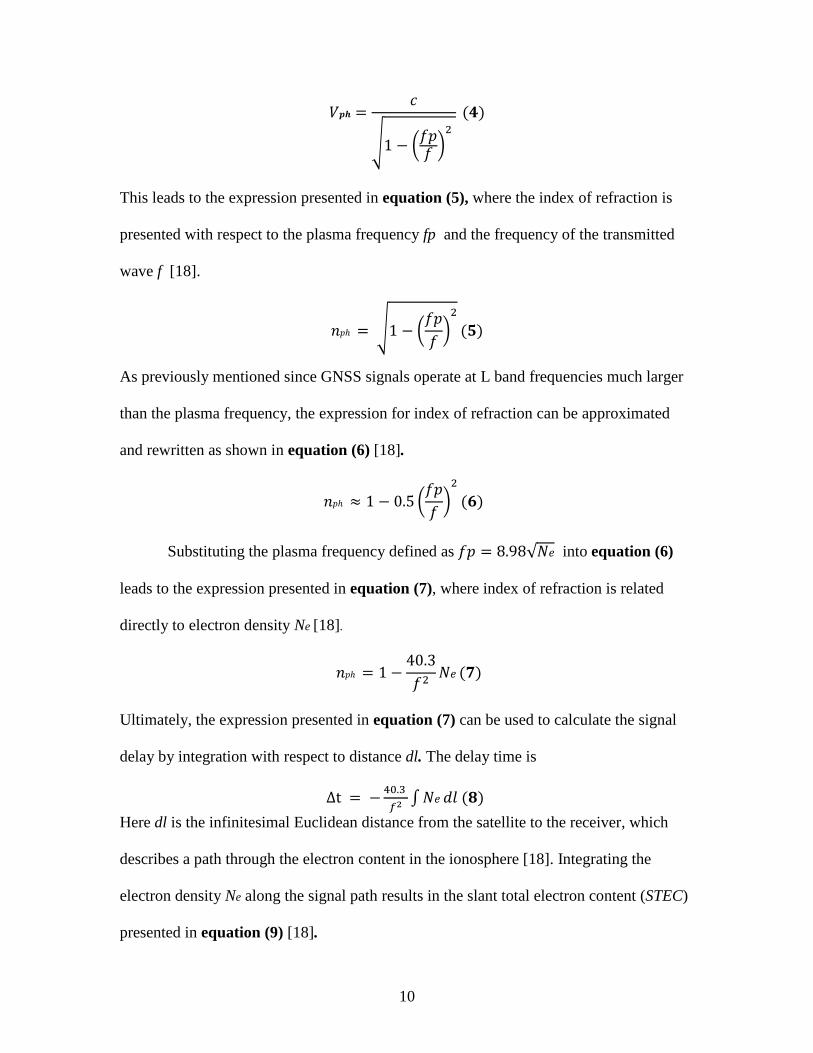
This leads to the expression presented in equation (5), where the index of refraction is
presented with respect to the plasma frequency fp and the frequency of the transmitted
wave f [18].
𝑛𝑝ℎ = √1 − (𝑓𝑝
𝑓)
2
(𝟓)
As previously mentioned since GNSS signals operate at L band frequencies much larger
than the plasma frequency, the expression for index of refraction can be approximated
and rewritten as shown in equation (6) [18].
𝑛𝑝ℎ ≈ 1 − 0.5 (𝑓𝑝
𝑓)
2
(𝟔)
Substituting the plasma frequency defined as 𝑓𝑝 = 8.98√𝑁𝑒 into equation (6)
leads to the expression presented in equation (7), where index of refraction is related
directly to electron density Ne [18].
𝑛𝑝ℎ = 1 −40.3
𝑓2𝑁𝑒 (𝟕)
Ultimately, the expression presented in equation (7) can be used to calculate the signal
delay by integration with respect to distance dl. The delay time is
∆t = −40.3
𝑓2 ∫ 𝑁𝑒 𝑑𝑙 (𝟖)
Here dl is the infinitesimal Euclidean distance from the satellite to the receiver, which
describes a path through the electron content in the ionosphere [18]. Integrating the
electron density Ne along the signal path results in the slant total electron content (STEC)
presented in equation (9) [18].

11
𝑆𝑇𝐸𝐶 = ∫ 𝑁𝑒 𝑑𝑙 (𝟗)
The total electron content in the Ionosphere can cause GNSS signals to be delayed
by 10’s of nano-seconds (ns) as they travels to the receiver [9]. Ionospheric delay in the
signal causes errors in pseudorange, which results in navigational solution errors.
Currently ionospheric delay is the largest source of GNSS positioning error.
The errors involved with the time delay can be almost eliminated by using
multiple frequencies in GNSS receivers. The time delay can also be calculated using
pseudorange values from dual frequency bands. Equation (10) describes the difference in
time delay between L1 and L2 frequency bands as shown
𝛥𝑡 =𝑃𝐿2−𝑃𝐿1
𝐶 (10)
obtained by taking the difference of the Pseudoranges on each frequency band (𝑃𝐿2 −
𝑃𝐿1) and dividing by the speed of light C. The time delay can be used to correct the error
in the Pseudorange. Note for simplicity for the discussion here equation (10) does not
incorporate error sources associated with the pseudorange measurements [9].
The time delay can be substituted into equation (11), to solve for the total
electron content (TEC) [9]. The TEC is dependent on the time delay 𝛥𝑡, speed of light C,
and the dual frequencies as shown
𝑇𝐸𝐶 =𝛥𝑡∗𝐶∗𝑓𝐋𝟏
2∗𝑓𝐋𝟐2
40.3∗(𝑓𝐋𝟏2−𝑓𝐋𝟐2) (11)
TEC is usually scaled with respect to total electron units (TECU), where 1 TECU =
1016 𝑒/𝑚2 [18].
12
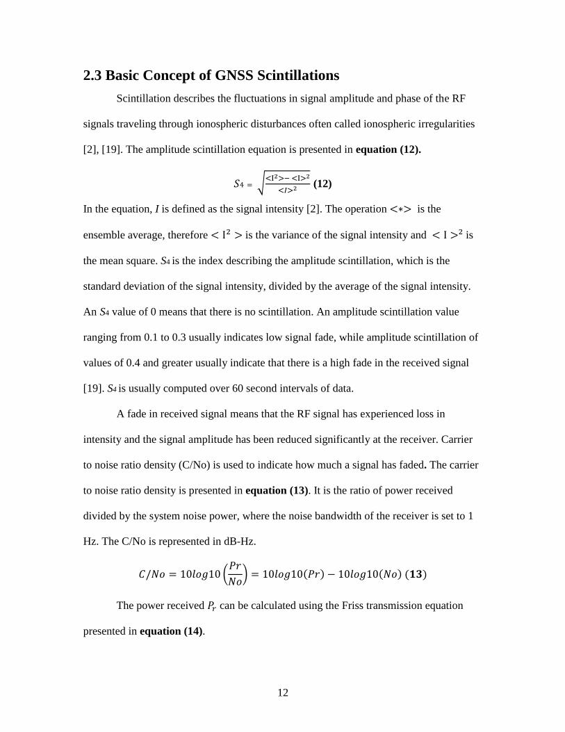
2.3 Basic Concept of GNSS Scintillations
Scintillation describes the fluctuations in signal amplitude and phase of the RF
signals traveling through ionospheric disturbances often called ionospheric irregularities
[2], [19]. The amplitude scintillation equation is presented in equation (12).
𝑆4 = √<I2>− <I>2
<𝐼>2 (12)
In the equation, I is defined as the signal intensity [2]. The operation <∗> is the
ensemble average, therefore < I2 > is the variance of the signal intensity and < I >2 is
the mean square. S4 is the index describing the amplitude scintillation, which is the
standard deviation of the signal intensity, divided by the average of the signal intensity.
An S4 value of 0 means that there is no scintillation. An amplitude scintillation value
ranging from 0.1 to 0.3 usually indicates low signal fade, while amplitude scintillation of
values of 0.4 and greater usually indicate that there is a high fade in the received signal
[19]. S4 is usually computed over 60 second intervals of data.
A fade in received signal means that the RF signal has experienced loss in
intensity and the signal amplitude has been reduced significantly at the receiver. Carrier
to noise ratio density (C/No) is used to indicate how much a signal has faded. The carrier
to noise ratio density is presented in equation (13). It is the ratio of power received
divided by the system noise power, where the noise bandwidth of the receiver is set to 1
Hz. The C/No is represented in dB-Hz.
𝐶/𝑁𝑜 = 10𝑙𝑜𝑔10 (𝑃𝑟
𝑁𝑜) = 10𝑙𝑜𝑔10(𝑃𝑟) − 10𝑙𝑜𝑔10(𝑁𝑜) (𝟏𝟑)
The power received 𝑃𝑟 can be calculated using the Friss transmission equation
presented in equation (14).
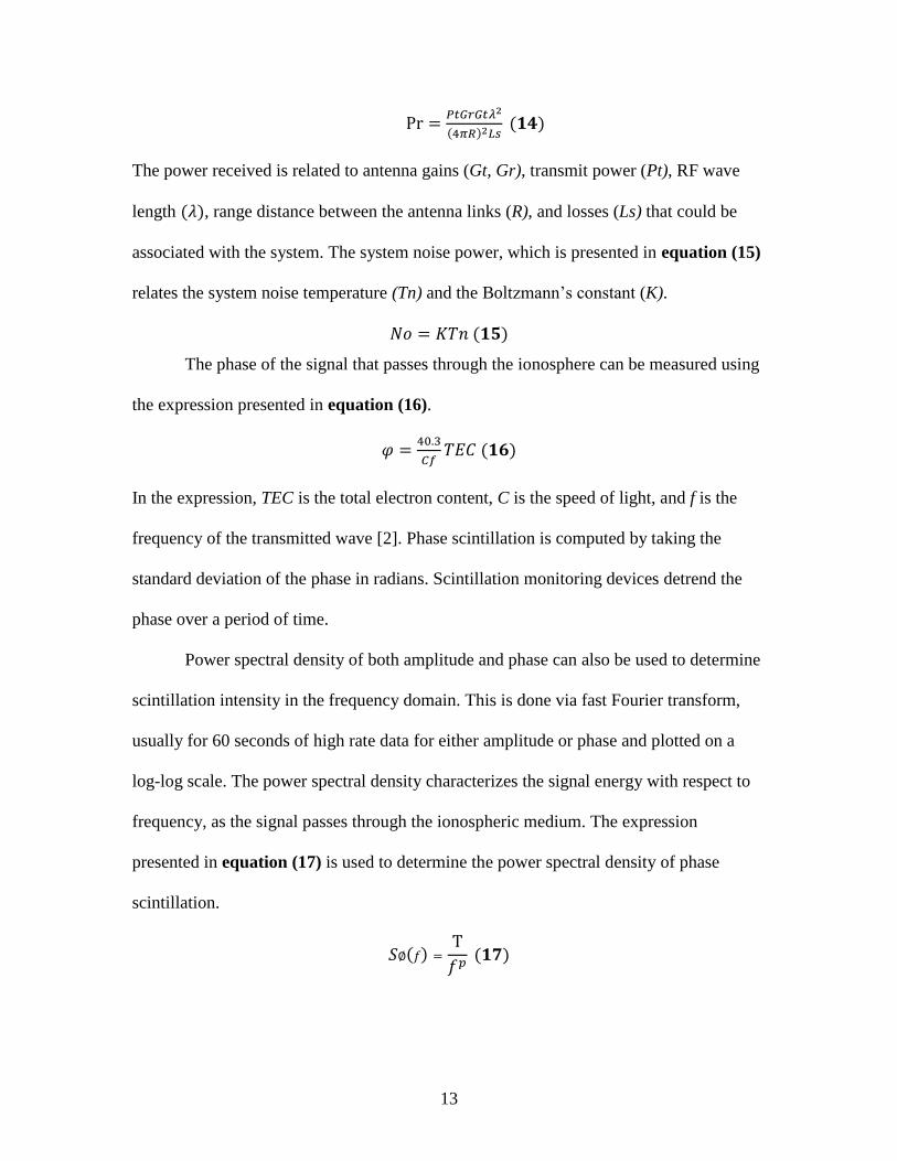
13
Pr =𝑃𝑡𝐺𝑟𝐺𝑡𝜆2
(4𝜋𝑅)2𝐿𝑠 (𝟏𝟒)
The power received is related to antenna gains (Gt, Gr), transmit power (Pt), RF wave
length (𝜆), range distance between the antenna links (R), and losses (Ls) that could be
associated with the system. The system noise power, which is presented in equation (15)
relates the system noise temperature (Tn) and the Boltzmann’s constant (K).
𝑁𝑜 = 𝐾𝑇𝑛 (𝟏𝟓)
The phase of the signal that passes through the ionosphere can be measured using
the expression presented in equation (16).
𝜑 =40.3
𝐶𝑓𝑇𝐸𝐶 (𝟏𝟔)
In the expression, TEC is the total electron content, C is the speed of light, and f is the
frequency of the transmitted wave [2]. Phase scintillation is computed by taking the
standard deviation of the phase in radians. Scintillation monitoring devices detrend the
phase over a period of time.
Power spectral density of both amplitude and phase can also be used to determine
scintillation intensity in the frequency domain. This is done via fast Fourier transform,
usually for 60 seconds of high rate data for either amplitude or phase and plotted on a
log-log scale. The power spectral density characterizes the signal energy with respect to
frequency, as the signal passes through the ionospheric medium. The expression
presented in equation (17) is used to determine the power spectral density of phase
scintillation.
𝑆∅(𝑓) =T
𝑓𝑝 (𝟏𝟕)
14
T represents the power density of the signal at 1 Hz and variable f represents the desired
frequency range [2], [19]. The phase power spectral density slope is greatly reduced at a
lower cut off frequency [19]. Everything past the lower cut off is referred to as the noise
floor [2], [19]. For the power spectral density of the phase, the lower cut off frequency is
dependent on the GNSS receiver phase lock loop bandwidth, which is usually set to 10
Hz [19]. Anything past the bandwidth of the receivers phase lock look bandwidth is
considered to be the noise. The variable p represents the slope of the line, which is
approximated from a linear fit curve in the power region. The power region is between
the low cut off frequency and noise floor cut off frequency of the power spectral density
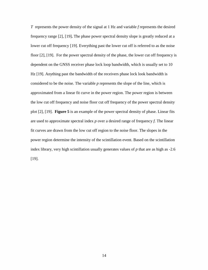
plot [2], [19]. Figure 5 is an example of the power spectral density of phase. Linear fits
are used to approximate spectral index p over a desired range of frequency f. The linear
fit curves are drawn from the low cut off region to the noise floor. The slopes in the
power region determine the intensity of the scintillation event. Based on the scintillation
index library, very high scintillation usually generates values of p that are as high as -2.6
[19].
15
Figure 5: Power spectral density of phase. Linear fit curves are drawn in the power region
between the low cut off region and high cut off region over desired frequency range f. The
spectral index p is approximated from the linear fit [1]
The amplitude intensity and phase power spectral densities are similar in that
they both have cut off frequencies at the noise floor [2]. The main difference between the
power spectral density of the amplitude and the phase is that the amplitude power spectral
density has a cut off frequency, referred to as the Fresnel frequency. Fresnel zones
describe the constructive and destructive interference boundaries of signals transmitted to
a receiver [16]. Transmitted signals can travel by line of sight (LOS) and also reflect or
diffract off surfaces. The total distance that the wave travels, which is the LOS distance
with the reflected or diffracted distance, can cause both constructive and destructive
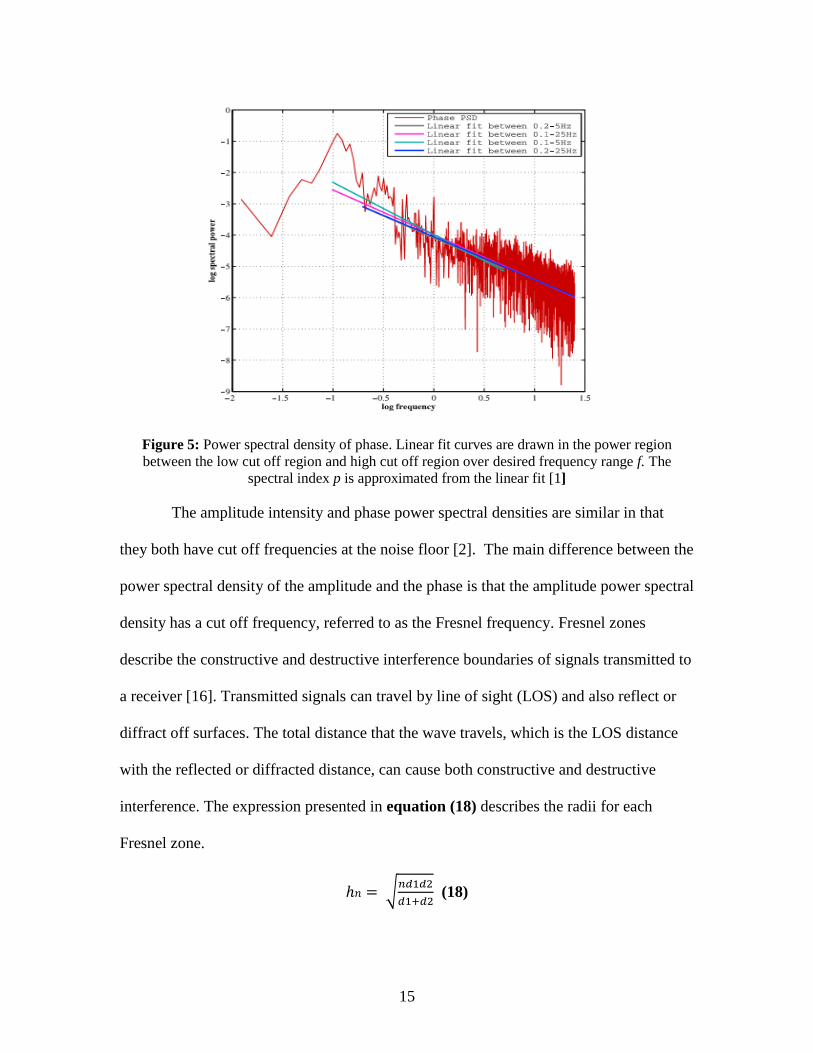
interference. The expression presented in equation (18) describes the radii for each
Fresnel zone.
ℎ𝑛 = √𝑛𝑑1𝑑2
𝑑1+𝑑2 (18)
16
In the equation d1 is the distance from the transmitter to point of reflection or diffraction
and d2 is the distance from point of reflection or diffraction to the receiver. The variable
n are integer values that can either be even or odd. Odd values of n define destructive
Fresnel frequency zones, while even values define constructive interference zones. Since
ionospheric disturbances cause GNSS signals to refract and bend, this can cause
destructive and constructive interference at the GNSS receiver.
As shown in Figure 10, the Fresnel frequency is defined by the cut off at which
the signal intensity begins to roll off and vary [2]. Fresnel frequency can be defined by
equation (19).
𝐹𝑓 = Vr
√2 𝜆𝑟 (𝟏𝟗)
It is related to the relative velocity between the satellite and ionospheric irregularities and
the wavelength of the signal. Lower case r in the equation is the distance between the
irregularities and GPS receiver [2].
To approximate spectral index p from the power spectral density of amplitude a
linear fit has to be drawn in the power region, which is between the Fresnel cut off
frequency and noise floor cut off frequency. Figure 10 is an example of a linear fit done
on the power spectral density of amplitude. A curve is drawn in the power region, which
is between the Fresnel frequency and noise floor.
It has been shown from past research that at low latitudes, amplitude scintillation
is more severe than phase scintillation, and at high latitudes, phase scintillation is more
severe than the amplitude scintillation [1]. One of the goals of this investigation is to
determine the severity of amplitude and phase scintillation at mid-latitude.
17
2.4 Past Scintillation Investigations
2.4.1 Low Latitudes
Studies have been done on GPS scintillation at low latitudes by a number of
researchers [20]. GPS scintillation data has been collected in Brazil near the equator.
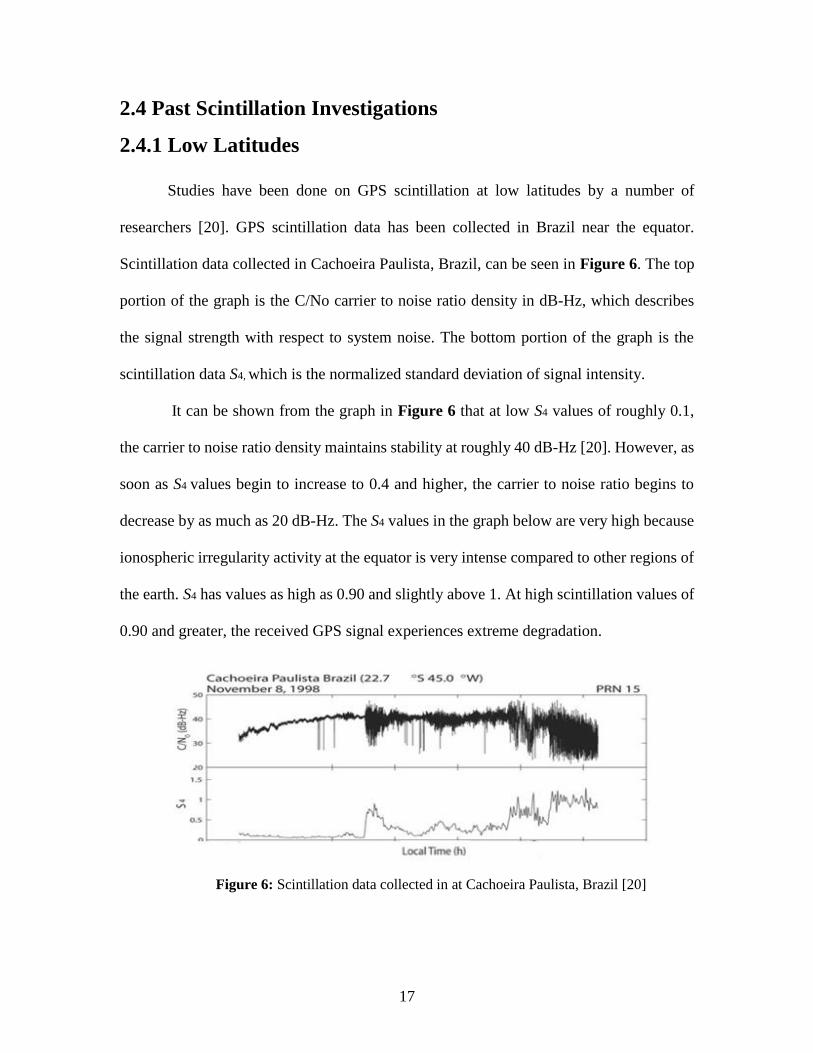
Scintillation data collected in Cachoeira Paulista, Brazil, can be seen in Figure 6. The top
portion of the graph is the C/No carrier to noise ratio density in dB-Hz, which describes
the signal strength with respect to system noise. The bottom portion of the graph is the
scintillation data S4, which is the normalized standard deviation of signal intensity.
It can be shown from the graph in Figure 6 that at low S4 values of roughly 0.1,
the carrier to noise ratio density maintains stability at roughly 40 dB-Hz [20]. However, as
soon as S4 values begin to increase to 0.4 and higher, the carrier to noise ratio begins to
decrease by as much as 20 dB-Hz. The S4 values in the graph below are very high because
ionospheric irregularity activity at the equator is very intense compared to other regions of
the earth. S4 has values as high as 0.90 and slightly above 1. At high scintillation values of
0.90 and greater, the received GPS signal experiences extreme degradation.
Figure 6: Scintillation data collected in at Cachoeira Paulista, Brazil [20]
18
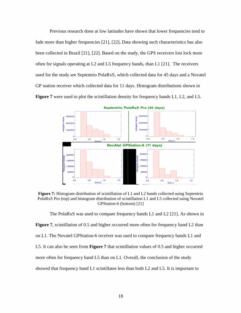
Previous research done at low latitudes have shown that lower frequencies tend to
fade more than higher frequencies [21], [22]. Data showing such characteristics has also
been collected in Brazil [21], [22]. Based on the study, the GPS receivers lost lock more
often for signals operating at L2 and L5 frequency bands, than L1 [21]. The receivers
used for the study are Septentrio PolaRxS, which collected data for 45 days and a Novatel
GP station receiver which collected data for 11 days. Histogram distributions shown in
Figure 7 were used to plot the scintillation density for frequency bands L1, L2, and L5.
Figure 7: Histogram distribution of scintillation of L1 and L2 bands collected using Septentrio
PolaRxS Pro (top) and histogram distribution of scintillation L1 and L5 collected using Novatel
GPStation-6 (bottom) [21]
The PolaRxS was used to compare frequency bands L1 and L2 [21]. As shown in
Figure 7, scintillation of 0.5 and higher occurred more often for frequency band L2 than
on L1. The Novatel GPStation-6 receiver was used to compare frequency bands L1 and
L5. It can also be seen from Figure 7 that scintillation values of 0.5 and higher occurred
more often for frequency band L5 than on L1. Overall, the conclusion of the study
showed that frequency band L1 scintillates less than both L2 and L5. It is important to

19
note that when this study was done back in 2012, only three satellites transmitted
frequency band L5 and ten satellites transmitted frequency band L2.
2.4.2 High Latitudes
Studies have been done on scintillation at high latitude regions in Lonyearbyen,
Norway [1]. For this study, both phase and amplitude power spectral densities were
analyzed in the frequency domain. The power spectral density of the phase is used to
determine spectral index p, since phase scintillation is considered to be more severe at
high latitudes and the power spectral density is used to determine the Fresnel frequency.
Figure 8 is an example of the power spectral density graph of both the phase in
green and the amplitude in blue, collected in Lonyearbyen, Norway [1]. As shown in the
figure, the phase and the amplitude power spectral densities have a similar frequency
power spectral variation. Figure 9 is a plot of spectral index p varying with respect to
time. The spectral index p was determined by linear interpolating the power spectral
density of the phase. As shown on the plot, p can vary from values less than 1 to values
as high as 3.5.
Figure 8: Power spectral density of amplitude and phase scintillation, green representing phase
and blue representing amplitude. Both data sets were collected at Lonyearbyen, Norway [1]
20
Figure 9: Linear interpolation of spectral index p over time. As shown on the plot above, p can
vary from values less than 1 to values as high as 3.5 [1]
2.4.3 Mid Latitudes
Few scintillation studies have been done at mid latitude regions. It is believed that
mid-latitude scintillation is negligible [1]. Some recent studies were performed at mid-
latitudes at the GPS laboratory at Virginia Tech in Blacksburg, VA [2]. Based on the
studies done, it was shown that at mid-latitude regions severe amplitude scintillation can
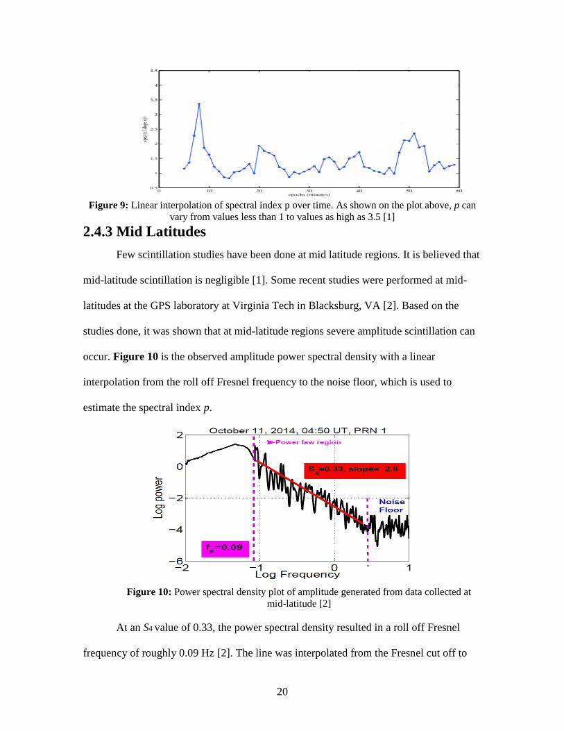
occur. Figure 10 is the observed amplitude power spectral density with a linear
interpolation from the roll off Fresnel frequency to the noise floor, which is used to
estimate the spectral index p.
Figure 10: Power spectral density plot of amplitude generated from data collected at
mid-latitude [2]
At an S4 value of 0.33, the power spectral density resulted in a roll off Fresnel
frequency of roughly 0.09 Hz [2]. The line was interpolated from the Fresnel cut off to
21
the noise floor cut off. The slope of the line was estimated to be -2.8. Based on these
findings it is shown that significant scintillation may occur at mid latitudes.
2.4.4 Summary
Based on the previous studies mentioned, it is clear that phase scintillation can be
severe reaching spectral index p values of up to 3.5, as shown in Figure 9 [1]. The
severity of amplitude scintillation at low-latitude during the scintillation event can be
seen in Figure 6. During this event, amplitude scintillation reached levels of 0.90 and
greater, which severely degraded the receiver carrier to noise ratio density [20]. It is
shown from Figure 10, from the power spectral density of amplitude, that scintillation
can be significant at mid-latitudes, with a spectral index p of -2.8 [2].
Based on the histogram distributions shown in Figure 7, it can be seen that L1
typically has lower S4 values compared to L2 and L5 at low latitudes. One of the main
motivations for this research is to determine which is more effected at mid-latitude, phase
or amplitude scintillation. Another goal is to determine which GNSS frequency bands are
likely to have lower amplitude and phase scintillation at mid-latitudes.
Chapter 3 Experimental Approach
3.1 GNSS Receiver
The scintillation data for this research was collected using a Novatel GP-6 GPS
receiver. Novatel GP-6 is capable of computing scintillation, carrier to noise ratio, and
phase of all the GPS satellite signals that it tracks. The Novatel GP-6 system used for
experimental observations in this work has ability to track signals from three GNSS
constellations. These constellations include GPS, GLONASS, and Galileo. The Novatel
GP-6 station is shown in Figure 11.

22
Figure 11: Current GP-6 station used at the Virginia Tech GPS lab [23]
The GP-6 station receiver can collect both high rate and low rate data. Both the
high rate and low rate data are collected at 50 Hz sampling rate or 50 samples per second
[23]. The low rate data includes computed amplitude scintillation, phase scintillation in
radians, carrier to noise ratio density in dB-Hz, and satellite elevation and azimuth angles
for each tracked satellite. The amplitude and phase scintillation are reduced and
detrended over 60 seconds of data, which corresponds to 3,000 data points. The phase is
first detrended using a 6th order Butterworth high pass filter. The statistics of the residuals
of the previous 60 seconds worth of data (3,000 data points) are computed over periods of
1 second, 3 seconds, 10 seconds, 30 seconds, and 60 seconds of phase sigma. The
amplitude is detrended by normalization over 60 seconds, or 3,000 data points.
High rate data generated by the receiver includes the measured power that is
relative to the base power, and is computed from the I and Q channels of the receiver
[23]. Since the measured power is relative to the base power it is unitless. The phase is
computed using Accumulated Doppler Range (ADR) data for every 0.02 seconds of data,
which corresponds to 50 Hz sampling rate. The high rate data provides the phase in mili
cycles.
Novatel GNSS receivers have a software interface called Novatel Connect.
Novatel Connect is used to communicate with the receiver, using a windows computer
23
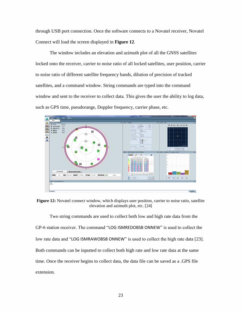
through USB port connection. Once the software connects to a Novatel receiver, Novatel
Connect will load the screen displayed in Figure 12.
The window includes an elevation and azimuth plot of all the GNSS satellites
locked onto the receiver, carrier to noise ratio of all locked satellites, user position, carrier
to noise ratio of different satellite frequency bands, dilution of precision of tracked
satellites, and a command window. String commands are typed into the command
window and sent to the receiver to collect data. This gives the user the ability to log data,
such as GPS time, pseudorange, Doppler frequency, carrier phase, etc.
Figure 12: Novatel connect window, which displays user position, carrier to noise ratio, satellite
elevation and azimuth plot, etc. [24]
Two string commands are used to collect both low and high rate data from the
GP-6 station receiver. The command “LOG ISMREDOBSB ONNEW” is used to collect the
low rate data and “LOG ISMRAWOBSB ONNEW” is used to collect the high rate data [23].
Both commands can be inputted to collect both high rate and low rate data at the same
time. Once the receiver begins to collect data, the data file can be saved as a .GPS file
extension.
24
Novatel provides C code that can be used to convert the GPS file to excel data
files in .CSV format. The code itself can be initiated using a windows command prompt.
Two commands are used to convert the GPS files, one is called PARSERAW and the
other one is called PARSEREDUCED [23]. The PARSERAW command is used to
convert high rate data GPS files and PARSEREDUCED is used to convert low rate data
.GPS files. The .CSV files for low rate and high rate data are generated differently for the
tracked satellites. Low rate data files include data for every single tracked satellite in one
.CSV file, while high rate data generates individual .CSV files for each of the tracked
satellites. As a result, different coding schemes were used to process the high rate and
low rate data.
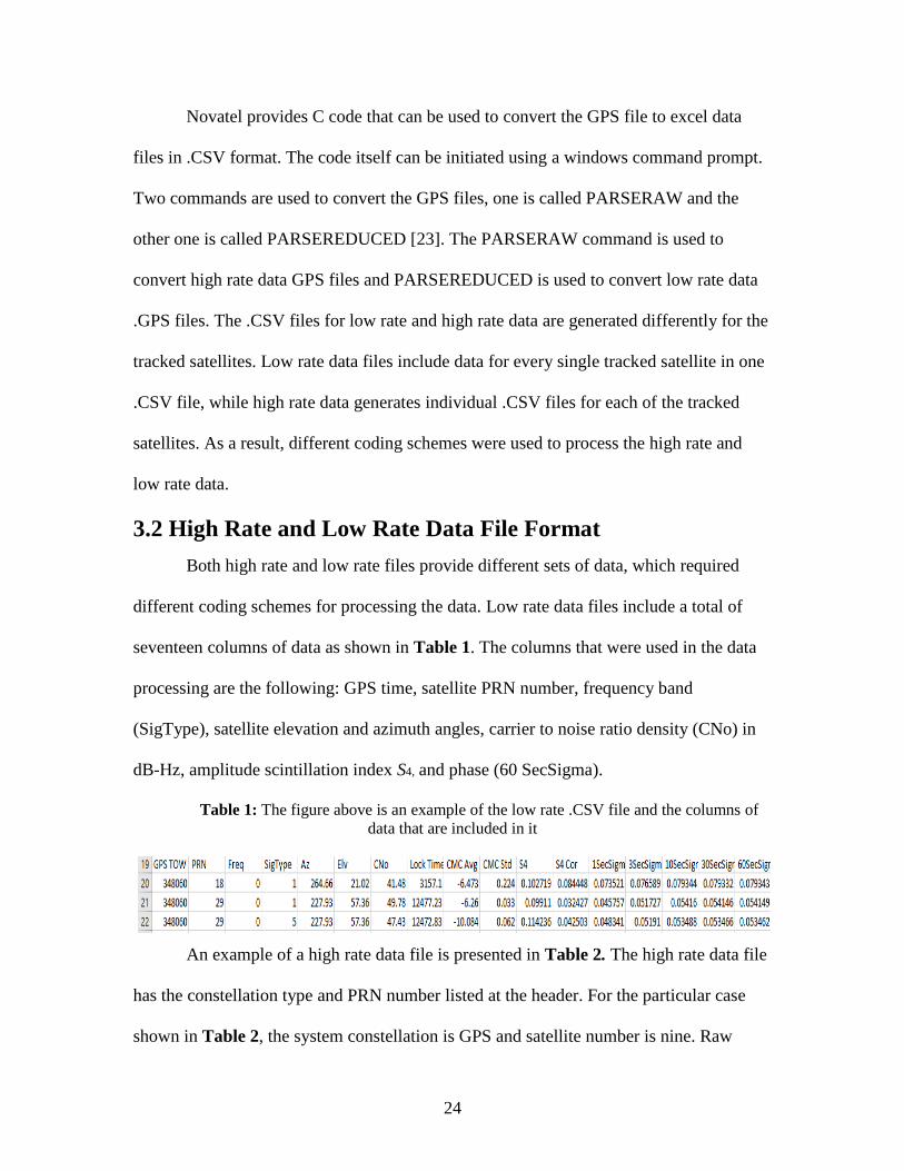
3.2 High Rate and Low Rate Data File Format
Both high rate and low rate files provide different sets of data, which required
different coding schemes for processing the data. Low rate data files include a total of
seventeen columns of data as shown in Table 1. The columns that were used in the data
processing are the following: GPS time, satellite PRN number, frequency band
(SigType), satellite elevation and azimuth angles, carrier to noise ratio density (CNo) in
dB-Hz, amplitude scintillation index S4, and phase (60 SecSigma).
Table 1: The figure above is an example of the low rate .CSV file and the columns of
data that are included in it
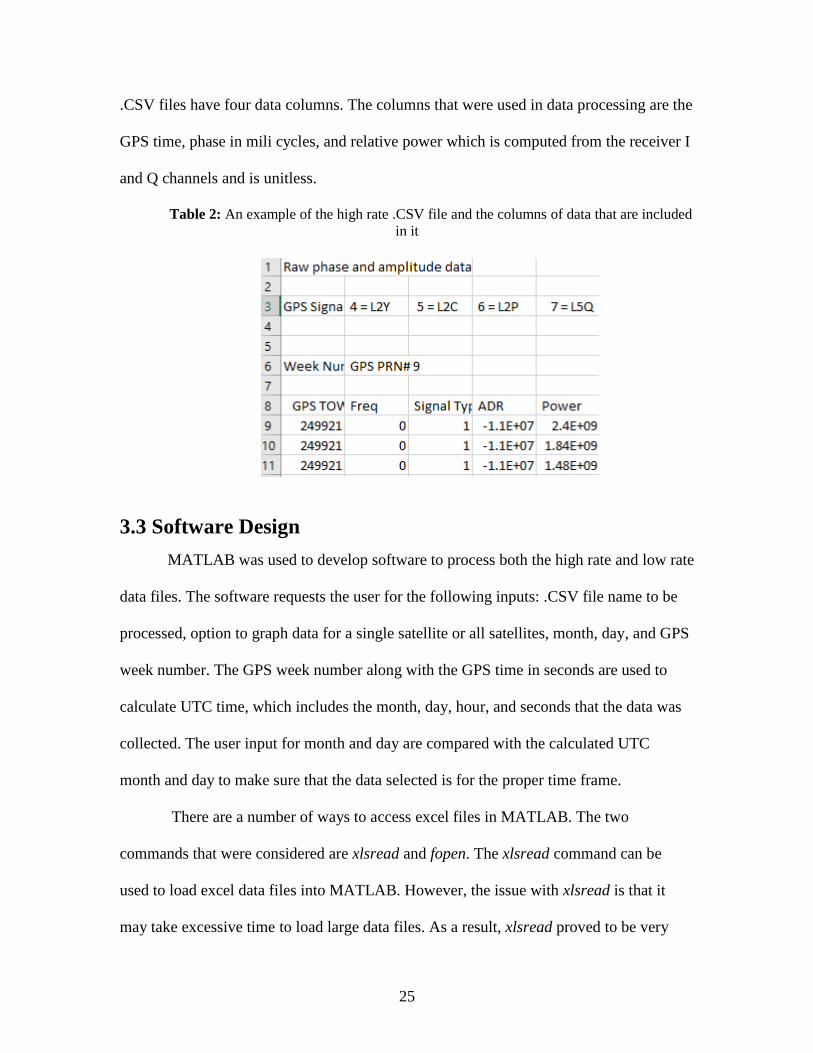
An example of a high rate data file is presented in Table 2. The high rate data file
has the constellation type and PRN number listed at the header. For the particular case
shown in Table 2, the system constellation is GPS and satellite number is nine. Raw
25
.CSV files have four data columns. The columns that were used in data processing are the
GPS time, phase in mili cycles, and relative power which is computed from the receiver I
and Q channels and is unitless.
Table 2: An example of the high rate .CSV file and the columns of data that are included
in it
3.3 Software Design
MATLAB was used to develop software to process both the high rate and low rate
data files. The software requests the user for the following inputs: .CSV file name to be
processed, option to graph data for a single satellite or all satellites, month, day, and GPS
week number. The GPS week number along with the GPS time in seconds are used to
calculate UTC time, which includes the month, day, hour, and seconds that the data was
collected. The user input for month and day are compared with the calculated UTC
month and day to make sure that the data selected is for the proper time frame.
There are a number of ways to access excel files in MATLAB. The two
commands that were considered are xlsread and fopen. The xlsread command can be
used to load excel data files into MATLAB. However, the issue with xlsread is that it
may take excessive time to load large data files. As a result, xlsread proved to be very
26
inefficient. Unlike xlsread, fopen doesn’t load the excel file data, but rather opens the file,
which saves time. As a result, this made accessing large amounts of data faster.
A number of steps had to be taken to access and store the data. For example, the
header information at the top of the .CSV file does not need to be stored, so a method had
to be implemented to skip over the header characters. A while loop and the fgetl
command were used to skip over the header characters. The MATLAB command fgetl is
used grab consecutive lines in a file that has been opened. As shown in Appendix 1, the
while loop had to be incremented nineteen times to skip over the header characters at the
top of the .CSV file. Since the header characters take up nineteen lines of space, the loop
had to be incremented nineteen times to reach the data.
The next step taken in the coding procedure was to determine the length of the
data file. When working with data files it is crucial to determine the length of the file in
order to identify the total number of lines of data in the file. This number is used to set a
limit on a looping method, used to process the whole data file. Shown in Appendix 1 is
the coding scheme used to determine the total number of lines in the .CSV file.
A while true loop is used to continuously loop through the file and fgetl is used to
grab the lines of data. The if condition in this code is used to identify the end of the file,
which doesn’t include any characters. As long as fgetl grabs a line which contains
characters, the variable size will continue to increment. Once the if condition is true for
no characters found at the end of the file, a break is used to break out of the while true
loop. The variable size will contain the total number of lines of data in the .CSV file.
The MATLAB command strread shown in Appendix 1 was used to scan and
store data for each row in the .CSV file. Strread can store a variety of data types, such as
27
floating numbers, decimal numbers, etc. Since the low rate data file has seventeen
columns of data, seventeen variables were used to store data for each scanned row. For
low rate data the variables that were stored are the following: GPS time in seconds,
satellite PRN number, frequency band of operation, azimuth and elevation satellite
angles, carrier to noise ratio density, scintillation index S4, and phase scintillation in
radians.
For high rate data, the textscan function shown in Appendix 1 was used to store
the GPS time in seconds, frequency band of operation, phase, and signal power. The
textscan function was used over strread because it was more efficient in processing larger
data files. The signal power is stored in sixty second intervals and used to compute
scintillation index S4, within that time frame. Phase is stored in mili cycle units and
converted to cycles. The format of strread command used to store the high rate data files
is presented in Appendix 1.
Chapter 4 Experimental Results
4.1 Introduction
For this study data is collected at mid-latitude from a GNSS receiver located in
Blacksburg, VA at 37.205 degrees latitude north and 80.417 degrees longitude west.
Observations were made on GNSS frequency bands L1, L2, L5, G1, G2, E1, E5A, and
E5B to conclude which band had better overall performance. The GNSS frequency band
observations are qualitatively compared to typical observations made at low latitudes in
Brazil [20], [21], [22]. Power spectral density of both amplitude and phase were used to
determine scintillation intensity by linear interpolation of slope p. The slope p values are
compared to previous mid-latitude observations from Blacksburg, VA and with p values

28
obtained from observations at high latitudes made in Lonyearbyen, Norway [1]. These
comparisons were made to investigate how mid-latitude scintillation characteristics in
general compare to those at low and high latitudes.
Three sets of data were collected on multiple days during severe and moderate
space weather conditions. The space weather was tracked by the space weather prediction
center, which uses magnetometers to make space weather predictions [25]. The space
weather prediction center provides daily Kp index values, which determine storm activity
over three hour intervals. A Kp index value which falls within a range of 4 to 9 indicates
that a geomagnetic storm is occurring. A Kp index value less than 4 is an indication of
moderate conditions. SuperDARN TEC and radar backscatter data, along with Kp index,
are used to show the conditions of the upper atmosphere while the data sets were
collected.
4.2 Data Set 1 Presentation
The first data set analyzed was collected on August 15th and 16th of 2015. During
this period of time a storm was tracked using the space weather prediction center. Figure
13 is a Kp index plot of the storm which occurred on August 15th and 16th of 2015. The
storm begins at 12:00 PM UTC time and continues through the 16th of August. As shown
on the plot, the Kp index value is as high as 7 and 6 when the storm begins and reduces to
a Kp value of 4 as it fades out on August the 16th.
Figure 14 is a TECU and radar backscatter plot generated by SuperDARN. As
shown, the TEC content varies from 7 to 12 TECU above Blacksburg, Virginia, where
the data was collected. The radar backscatter plot shows a SNR ranging from 10 to 20
dB, above Virginia.
29
Figure 13: Kp index plot of a small geomagnetic storm that occurred on August the 15th and
lasted until August the 16th [25]
Figure 14: Total electron and radar backscatter plots at 13:18:00 UTC of the geomagnetic storm
that occurred on August the 16th [7]
4.2.1 Scintillation Analysis
Low rate data was collected for data set 1. The scintillation index S4, carrier to
noise ratio density in dB-Hz, and phase in radians are presented for satellites from the
GPS, GLONASS, and Galileo constellations. The scintillation conditions were compared
across GPS frequency bands L1, L5, GLONASS G1, G2, and Galileo E1, E5A, and E5B.

30
It is important to note that the Galileo constellation is not completely filled at this time.
This is expected by 2020. During the time this data was taken in 2015, the receiver could
track at most four Galileo satellites which limited the Galileo data observations.
Figure 15: Elevation and azimuth plot of satellites analyzed during a turbulent event. The
satellites are represented, by red stars. GPS satellites 9, 27, GLONASS 14, 17, and Galileo 19 are
shown on the plots [26]
Figure 15 is an elevation and azimuth plot of the GNSS satellites analyzed during
the August the 16th storm. These are the locations of the satellites during the event which
occurred at 13:18:00 UTC time. This plot is meant to give a visual of the satellite
locations during the event. GPS satellites 9 and 27 and GLONASS 14 and 7 are fairly
close to one another. Galileo satellite 19 has a very low elevation angles compared to the
other observed satellites and is the farthest away. As a result, it is important to note that
Galileo satellite 19 may not have been effected by the turbulent events like the other
satellites, but may have been experiencing high amplitude scintillation at lower elevation
angles since there is a longer line of site (LOS). Since the GPS and GLONASS satellites
are relatively close to one another, this could have been the reason why all these satellites
experience severe amplitude and moderate phase scintillation at the same time frame. The
scintillation analysis is further discussed in this section.
31
Table 3 lists the satellite numbers, frequency bands, maximum amplitude
scintillation index S4, maximum phase scintillation, frequency bands, and satellite
location during the period of maximum scintillation. The majority of the observed
satellites are all above 15 degrees elevation angle to mitigate multipath effects. These
observations indicate that at mid-latitudes, scintillation can potentially be severe just as
low and high latitude regions. However, since this storm only lasted a short period of
time, the scintillation wasn’t prolonged.
Table 3: Data from August the 16th storm. S4, frequency bands, carrier to noise ratio, and change
in carrier to noise ratio, displayed below
Sat
Type
Sat
No
Freq
Band
Max
Amplitude
Index (S4)
Max
Phase
𝜑 (radians)
Azimuth
Angle
At Max
(S4)
Elevation
Angle
At Max
(S4)
GPS 9 L1 0.8139 0.354 236.56 47.93
GPS 9 L5 0.6528 0.262 236.56 47.93
GPS 27 L1 0.8425 0.350 52.81 51.84
GPS 27 L5 0.6350 0.260 52.81 51.84
GLONASS 14 G1 0.6098 0.374 48.88 56.25
GLONASS 14 G2 0.4598 0.289 48.88 56.25
GLONASS 17 G1 0.9142 0.373 150.00 58.29
GLONASS 17 G2 0.4236 0.307 150.00 58.29
Galileo 19 E1 0.3876 0.358 214.37 14.08
Galileo 19 E5A 0.5450 0.267 211.35 9.64
Galileo 19 E5B 0.5661 0.274 211.56 9.93

32
The satellites listed in Table 3, excluding Galileo satellite number 19, resulted in
severe scintillation at 13:18:00 UTC time. All the satellites listed in Table 3 experienced
maximum phase scintillation at 12:22:00 UTC time during a period in which amplitude
scintillation is low. GPS satellite numbers 9 and 27 at L1 frequency band and GLONASS
satellite number 17 at G1 frequency band resulted the highest amplitude scintillation
values of 0.8139, 0.8425, and 0.9142 for short periods of time. These values are
comparable to the low latitude scintillation values collected, by [20]. The highest phase
scintillation occurred on frequency bands L1, G1, and E1 across GPS, GLONASS, and
Galileo. The values were fairly close at 0.354 and 0.350 radians on GPS L1, 0.374 and
0.373 radians on GLONASS G1, and 0.358 radians on Galileo E1. The lowest
scintillation values occurred across bands GPS L5, GLONASS G2, and Galileo E5A,
E5B. These values are also relatively close. The max phase scintillation across L5 are
0.262 and 0.260 radians, 0.289 and 0.307 radians on GLONASS G2, and 0.267 and 0.274
on Galileo E5A and E5B.
The upper atmospheric disturbance that occurred at 13:18:00 UTC degraded
signals operating at the L1 and G1 frequency bands more severely than frequencies
transmitted at L2, G2, and L5. GPS satellites 9 and 27 had maximum amplitude
scintillation at L1 of 0.8139 and 0.8425, but had less amplitude scintillation at L5 of
0.6528 and 0.6350. GLONASS satellites 14 and 17 had maximum amplitude scintillation
at G1 of 0.6098 and 0.9142, but had less amplitude scintillation at G2 of 0.4598 and
0.4236. It is important to note that frequency band G2 had less amplitude scintillation
than L1, L5, and G1 during the time of the disturbance.

33
Unlike the other satellites, Galileo satellite number 19 had maximum scintillation
at E1, E5A, and E5B at different periods of time, but the time difference is relatively
small and it could be argued that the same atmospheric disturbance degraded the satellite
signal strength. Galileo satellite 19 had maximum amplitude scintillation of 0.3876 at
12:52:00 UTC for frequency band E1, 0.5450 at 13:07:00 UTC for frequency band E5A,
and 0.5661 at 13:06:00 UTC for frequency band E5B. These severe scintillation values
were collected at different elevation angles less than 15 degrees. As a result, multipath
errors could have likely contributed to the signal degradation.
Figure 16: Scintillation, carrier to noise ratio, and phase of GPS satellite PRN number 9, at
frequency L1

34
Figure 16 includes scintillation index S4, carrier to noise ratio density in dB-Hz,
and phase in radians of GPS satellite 9, for both L1 and L5 frequency bands. Low rate
data was graphed for a duration of four hours during the geomagnetic storm which
occurred on August 16th 2015. As shown in the figures, scintillation remains very low,
close to the value 0, for both frequency bands and peaks at 13:18:00 UTC during an
upper atmospheric disturbance event. It can also be shown from the figures that phase
scintillation changes by 0.1733 radians of phase scintillation for frequency band L1 and
0.1269 radians of phase scintillation for frequency band L5. The carrier to noise ratio
density of the signal is also effected on both frequency bands. L1 is reduced from roughly
50 dB-Hz to 41.85 dB-Hz and L5 is reduced from roughly 55 dB-Hz to 48.16 dB-Hz. L5
frequency band has a higher carrier to noise ratio density than L1 frequency band, which
resulted in better overall performance, during the disturbance. Based on the change of
phase scintillation during the turbulence L5 has less of a phase change than L1.
Figure 17: Scintillation, carrier to noise ratio, and phase of GPS satellite PRN number 27, at
frequency L1

35
Figure 18: Scintillation, carrier to noise ratio, and phase of GPS satellite PRN number 27, at
frequency L5
Figure 17 and Figure 18 show scintillation index S4, carrier to noise ratio density
in dB-Hz, and phase scintillation in radians of GPS satellite 27, for both L1 and L5
frequency bands. Low rate data was graphed for a duration of four hours during the
geomagnetic storm which occurred on August 16th 2015. Like GPS satellite 9, the L1 and
L5 frequency bands transmitted by satellite 27 maintained low amplitude scintillation
values of roughly 0 and peaked at 13:18:00 UTC during the upper atmospheric
disturbance event. The carrier to noise ratio density of L1 is reduced from roughly 50 dB-
Hz to 43.43 dB-Hz and L5 is reduced from roughly 55 dB-Hz to 50 dB-Hz. Like the
previous results from GPS satellite 9, data from GPS satellite 27 shows that L5 has a
better overall performance than L1. The phase scintillation during the turbulence at L1
was 0.2185 radians, while L5 was 0.1395 radians. Like the data from GPS satellite 9, this
data from satellite 27 also shows that the L5 signal phase was less effected by the
turbulence compared to the phase at L1.

36
Figure 19: Scintillation, carrier to noise ratio, and phase of GLONASS satellite PRN number 14,
at frequency G1
Figure 19 depicts graphs of scintillation index S4, carrier to noise ratio in dB-Hz,
and phase in radians of GLONASS satellite 14, for both G1 and G2 frequency bands.
Low rate data for this satellite was graphed for a duration of four hours. Like GPS
satellite number 9 and 27, GLONASS satellite 14 was effected by the disturbance at
13:18:00 UTC. As shown in the above figures, the amplitude scintillation peaks at
13:18:00 UTC. Frequency band G1 scintillates more than G2. For both frequency bands

37
the carrier to noise ratio density peaks at roughly 40 dB-Hz and the degradation of
performance is almost equivalent. The carrier to noise ratio density of G1 degrades to
37.46 dB-Hz, while G2 degrades to 38.42 dB-Hz. However, the change in phase
scintillation of G2 at 0.1537 radians is less than G1 at 0.2104 radians. As a result, the
overall performance of G2 is better than G1 during the turbulence.
Figure 20: Scintillation, carrier to noise ratio, and phase of GLONASS satellite PRN number 17,
at frequency G2
Figure 20 depicts graphs of scintillation index S4, carrier to noise ratio in dB-Hz,
and phase in radians of GLONASS satellite 17, for both G1 and G2 frequency bands. Low
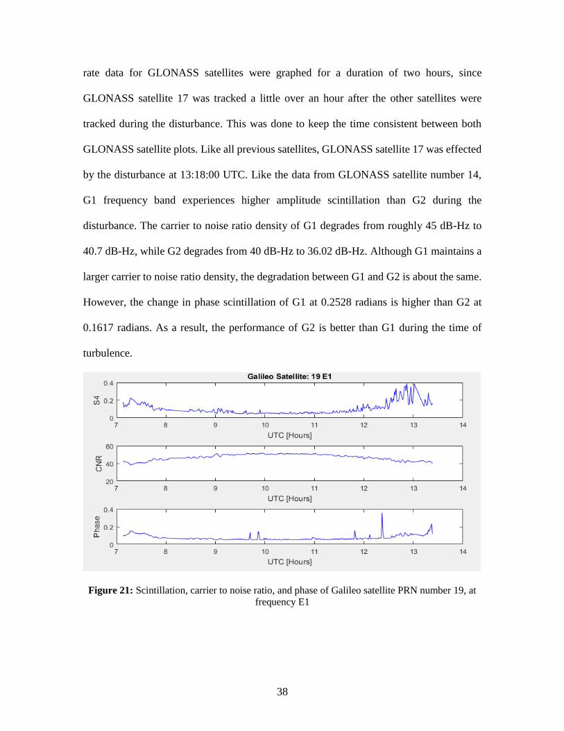
38
rate data for GLONASS satellites were graphed for a duration of two hours, since
GLONASS satellite 17 was tracked a little over an hour after the other satellites were
tracked during the disturbance. This was done to keep the time consistent between both
GLONASS satellite plots. Like all previous satellites, GLONASS satellite 17 was effected
by the disturbance at 13:18:00 UTC. Like the data from GLONASS satellite number 14,
G1 frequency band experiences higher amplitude scintillation than G2 during the
disturbance. The carrier to noise ratio density of G1 degrades from roughly 45 dB-Hz to
40.7 dB-Hz, while G2 degrades from 40 dB-Hz to 36.02 dB-Hz. Although G1 maintains a
larger carrier to noise ratio density, the degradation between G1 and G2 is about the same.
However, the change in phase scintillation of G1 at 0.2528 radians is higher than G2 at
0.1617 radians. As a result, the performance of G2 is better than G1 during the time of
turbulence.
Figure 21: Scintillation, carrier to noise ratio, and phase of Galileo satellite PRN number 19, at
frequency E1
39
Figure 22: Scintillation, carrier to noise ratio, and phase of Galileo satellite PRN number 19, at
frequency E5A and E5B
Figure 21 and Figure 22 are graphs of scintillation index S4, carrier to noise ratio
in dB-Hz, and phase in radians of Galileo satellite 19 at E1, E5A, and E5B. Galileo
satellite 19 experiences signal degradation from 12:00:00 UTC to around 13:06:00 UTC.
Within that time range, frequency band E1 experiences greater scintillation fluctuations
compared to frequency bands E5A and E5B. The carrier to noise ratio density of the
40
frequency bands diminish from 12:00:00 UTC to 13:06:00 UTC. The carrier to noise
ratio density of E1 degrades from 50 dB-Hz to 42.62 dB-Hz, while E5A from roughly 48
dB-Hz to 42.2 dB-Hz, and E5B from 48 dB-Hz to 42.01 dB-Hz. The carrier to noise ratio
density reduction is fairly the same across all three of these frequency bands during this
turbulent event caused by the geomagnetic storm or from a longer line of site (LOS). At
12:22:00 UTC time all three frequency bands experience a change of phase. E5A has a
change of phase of 0.2676 radians and E5B of 0.2747 radians, which is less than both E1
and E5B. During the disturbance, E1 had the worst performance of the three frequency
bands. E5A and E5B resulted in similar carrier to noise ratio density degradation and
change in phase scintillation. However, E5A had slightly better performance.
41
4.2.2 Summary
Figure 23: Histogram distribution of GPS satellite PRN 9 (L1, L5) and GPS satellite PRN 27
(L1, L5) scintillation above 15 degrees elevation angle
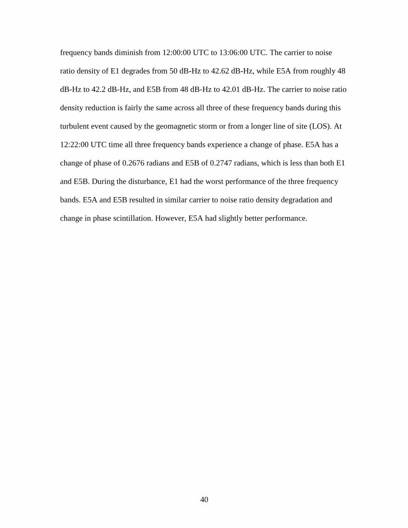
Figure 23 are histogram distributions of all amplitude scintillation data, above 15
degrees elevation angle, collected for GPS satellites 9 and 27 during the geomantic storm
from August the 15th to August the 16th, 2015. The histogram distributions show that
signals transmitted at L1 for both GPS satellites 9 and 27 have higher scintillation
occurrence, compared to frequency band L5. This validates the previous analysis done on
Figure 16 through Figure 18, which shows that signals transmitted on L5 experienced
less amplitude scintillation. These results are not in alignment with other observations
which indicate that L1 scintillated less than L5 [21]. However, the data analyzed for this
research is collected at mid-latitudes unlike the data collected at low latitudes, by [21].
The difference in upper atmospheric region could possibly be why L5 outperforms L1
and L2 at mid-latitude, but L1 outperforms L2 and L5 in low latitude regions [21].

42
For this data set, L5 maintains a greater carrier to noise ratio density than L1, so it
can be inferred that signals transmitted on L5 have greater received power than signals
transmitted on L1. It is shown that L5 increases to a maximum carrier to noise ratio
density of roughly 55 dB-Hz, while L1 increase to a maximum carrier to noise ratio
density of roughly 50 dB-Hz. In this case, L5 has 5 dB-Hz greater maximum carrier to
noise ratio density than L1. One of the factors that contributes to L5 having greater
carrier to noise ratio density is the fact that signals transmitted on L5 have 3 dB more
signal power than signals transmitted on L1 [27]. Having a greater transmit power may
reduce both amplitude and phase scintillation which leads to better overall carrier to noise
ratio performance. However, it is important to note that transmit power isn’t the only
factor in calculating the overall carrier to noise ratio density, other variables shown above
in equation (14), includes signal wave length, distance the signal traveled from
transmitter to receiver, and losses caused by the atmosphere. Since this data is collected
at mid-latitudes, the atmospheric losses are different from high and low latitudes. As a
result, the scintillation across the observed frequency bands will be affected differently.
Further observations will be discussed in Section 4.3 and Section 4.4.

43
Figure 24: Histogram distribution of GLONASS satellite (G1, G2) and GLONASS satellite 27
(G1, G2) scintillation above 15 degrees elevation angle
During the disturbed upper atmospheric conditions at 13:18:00 UTC, it is shown
from the analysis done on Figure 20, that G2 performs better than G1. However, the
histogram distribution of scintillation density in Figure 24, shows discrepancies between
GLONASS satellite 14 and 17. For Satellite 14, G2 scintillates less than G1 and for
satellite 17 G1 scintillates less than G2. The difference in scintillation could be due to
FDMA, which GLONASS uses. Since GLONASS is an FDMA system, each satellite in
view uses a different frequency band, to avoid interference with other neighboring
satellites. Since each frequency band is different, the scintillation may vary across each
band. As a result, variation in scintillation for G1 for satellite 14 is different for satellite
17 and the same can be said for G2. As a result, this makes GLONASS more difficult to
carefully analyze.
44
Other histogram plots that show the same discrepancies across GLONASS G1
and G2 are discussed in data set 3. GLONASS G1 and G2 do share a similar resemblance
in distribution. In data set 3, it is shown that G1 and G2 have similar amplitude and phase
scintillation. The correlation characteristics of both amplitude and phase scintillation
across G1 and G2 are further discussed in data set 3.
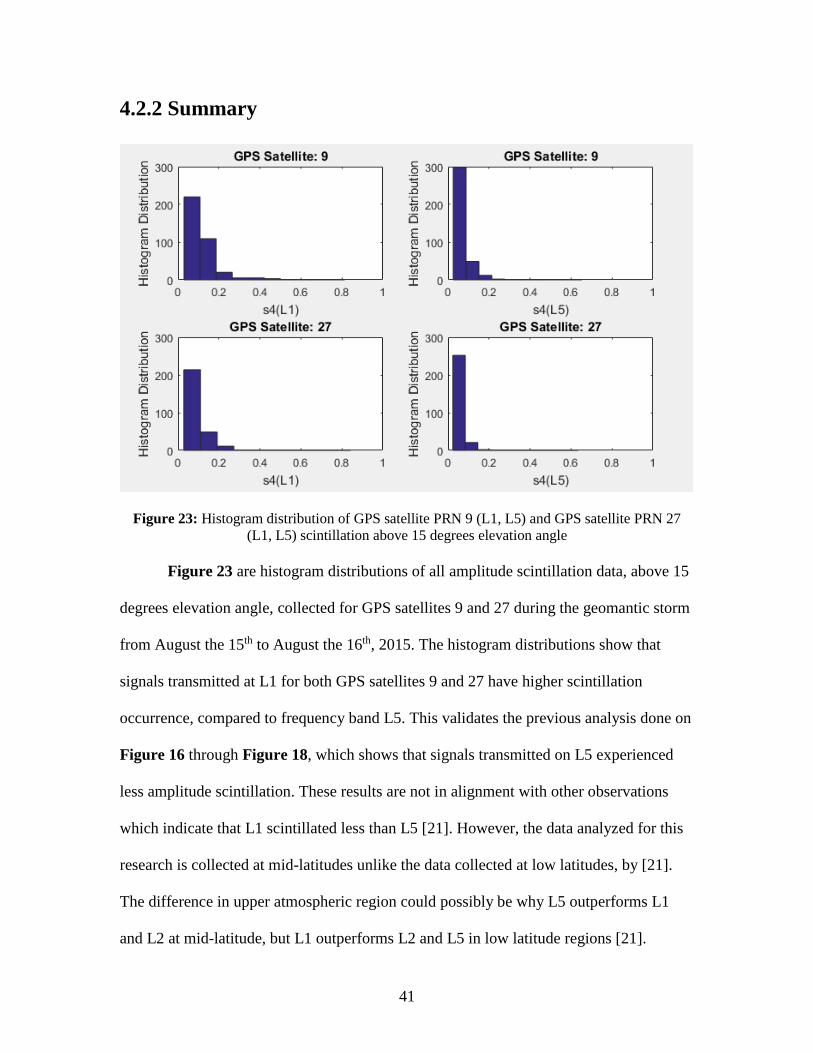
Figure 25: Histogram distribution of Galileo satellite 19 (E1, E5A, E5B) scintillation above 15
degrees elevation angle
Figure 25 is the scintillation distribution for Galileo satellite 19. Based on the
distribution E5A has a higher scintillation distribution compared to higher frequencies of
E1 and E5B. E1 and E5B both have similar distributions. However, E1 experiences
slightly less scintillation than E5B and less scintillation than E5A. E1 may have had less
scintillation than the other frequency bands, due to higher carrier to noise ratio density.
As shown in Figure 21 and Figure 22, E1 had a maximum carrier to noise ratio density

45
of roughly 50 dB-Hz, while E5A and E5B had a maximum carrier to noise ratio density
of 48 dB-Hz.
Based on the values listed in Table 3, the magnitude of amplitude scintillation is
higher than the magnitude of phase scintillation. The highest amplitude scintillation was
0.9142 and the highest phase scintillation was 0.373 radians. From these values it appears
that amplitude scintillation is more severe at mid-latitudes than phase scintillation.
4.3 Data Set 2 Presentation
The second set of data was taken during a geomagnetic storm, on February 16th,
2016. As shown in Figure 26, the storm begins at 12:00:00 PM UTC and lasts up till
February 17th 3:00:00 AM UTC. The storm maintains a Kp index of 5 and peeks at an
index of 6 at 18:00:00 UTC. Like the storm from data set 1, data set 2 shows electron
content ranging from 7 to 12 TECU, shown in Figure 27. Unlike the back scatter from
data set 1, the back scatter of data set 2 is not as strong above Virginia, shown in Figure
27. The small concentration of scatter resulted in a SNR ranging from 10 to 20 dB.
Figure 26: Kp index plot of a small geomagnetic storm that occurred on February the 16th and
lasted until February the 17th [25]
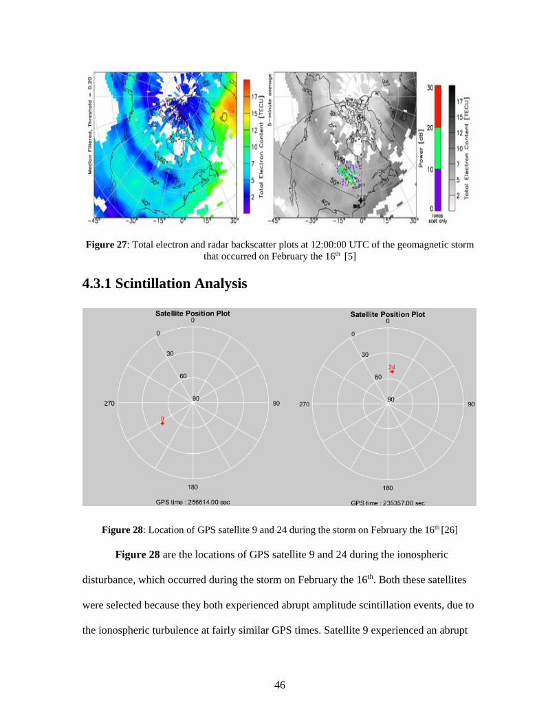
46
Figure 27: Total electron and radar backscatter plots at 12:00:00 UTC of the geomagnetic storm
that occurred on February the 16th [5]
4.3.1 Scintillation Analysis
Figure 28: Location of GPS satellite 9 and 24 during the storm on February the 16th [26]
Figure 28 are the locations of GPS satellite 9 and 24 during the ionospheric
disturbance, which occurred during the storm on February the 16th. Both these satellites
were selected because they both experienced abrupt amplitude scintillation events, due to
the ionospheric turbulence at fairly similar GPS times. Satellite 9 experienced an abrupt

47
scintillation at GPS time of 256614 seconds and satellite 24 at 235357 seconds. These
two satellites are used to further validate abrupt amplitude scintillation events at mid-
latitude. Since high rate data doesn’t include the satellite elevation and azimuth angles,
STK software tool [28] was used to determine the location of these satellites during the
turbulent event. Both satellites had elevation angles above 15 degrees during the event.
Satellite 9 had an elevation angle of 46.43 degrees and satellite 24 had an elevation angle
of 51.722 degrees.
High rate data was collected for data set 2. The high rate 50 Hz data includes the
signal power, which is computed from the I and Q channels and is unitless, since it is
relative to the base power. The signal power is plotted on a logarithmic scale defined by
𝑆𝑖𝑔𝑛𝑎𝑙 𝑃𝑜𝑤𝑒𝑟 = 10 ∗ 𝑙𝑜𝑔10(𝐼2 + 𝑄2). The phase of the high rate data is in units of
millicycles. The high rate signal power is graphed for GPS L1, L2, L5, GLONASS G1,
G2, and Galileo E1, E5A, E5B to determine which frequency bands are more prone to
fading.
High rate data is used to compute spectral index p using the amplitude signal
power, since it is shown in data set 1 that amplitude scintillation is more severe than
phase scintillation. Only a few satellites were selected from each constellation to
determine spectral index p during maximum amplitude scintillation events. These results
were found to be representative of the larger group of satellites tracked. Nonetheless, it is
important to note that more studies need to be done in the future to further investigate
spectral index p and to further observe the variations of signal power across the frequency
bands analyzed in this study.
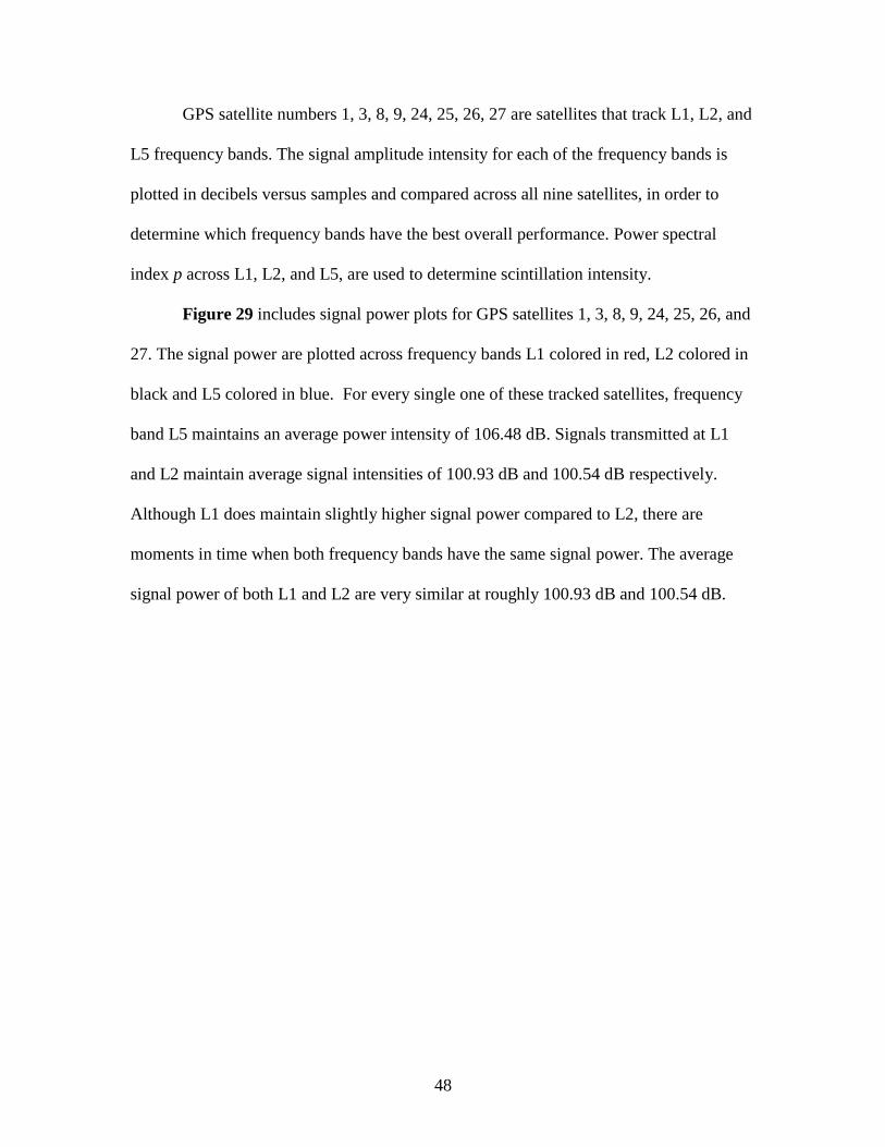
48
GPS satellite numbers 1, 3, 8, 9, 24, 25, 26, 27 are satellites that track L1, L2, and
L5 frequency bands. The signal amplitude intensity for each of the frequency bands is
plotted in decibels versus samples and compared across all nine satellites, in order to
determine which frequency bands have the best overall performance. Power spectral
index p across L1, L2, and L5, are used to determine scintillation intensity.
Figure 29 includes signal power plots for GPS satellites 1, 3, 8, 9, 24, 25, 26, and
27. The signal power are plotted across frequency bands L1 colored in red, L2 colored in
black and L5 colored in blue. For every single one of these tracked satellites, frequency
band L5 maintains an average power intensity of 106.48 dB. Signals transmitted at L1
and L2 maintain average signal intensities of 100.93 dB and 100.54 dB respectively.
Although L1 does maintain slightly higher signal power compared to L2, there are
moments in time when both frequency bands have the same signal power. The average
signal power of both L1 and L2 are very similar at roughly 100.93 dB and 100.54 dB.
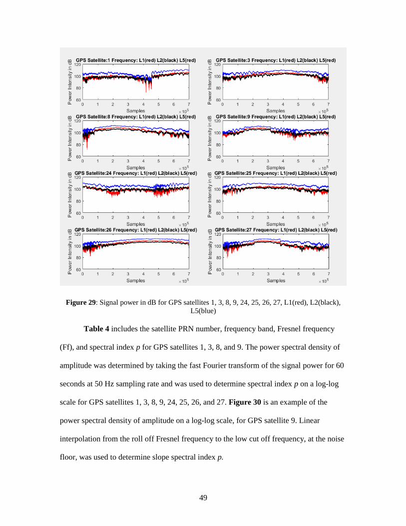
49
Figure 29: Signal power in dB for GPS satellites 1, 3, 8, 9, 24, 25, 26, 27, L1(red), L2(black),
L5(blue)
Table 4 includes the satellite PRN number, frequency band, Fresnel frequency
(Ff), and spectral index p for GPS satellites 1, 3, 8, and 9. The power spectral density of
amplitude was determined by taking the fast Fourier transform of the signal power for 60
seconds at 50 Hz sampling rate and was used to determine spectral index p on a log-log
scale for GPS satellites 1, 3, 8, 9, 24, 25, 26, and 27. Figure 30 is an example of the
power spectral density of amplitude on a log-log scale, for GPS satellite 9. Linear
interpolation from the roll off Fresnel frequency to the low cut off frequency, at the noise
floor, was used to determine slope spectral index p.

50
Table 4: GPS Satellite Numbers 1, 3, 8, 9, Frequency Bands, Fresnel Frequency (Ff), and
Spectral Index p
Table 5 includes the satellite numbers, frequency band, Fresnel frequency (Ff),
and spectral index p for GPS satellites 24, 25, 26, and 27. The spectral index p vary
between values from -1.179 to -2.621. The average spectral index p across L1, L2C, and
L5 from Table 4 and Table 5 is -1.922.
Satellite PRN
Number
Frequency
Band
Ff
(Hz)
Spectral
Index p
Max
Scintillation
1 L1 0.066 -2.02 0.4437
1 L2C 0.08 -1.393 0.2993
1 L5 0.10 -1.644 0.2937
3 L1 0.15 -2.621 0.848
3 L2C 0.10 -1.699 0.429
3 L5 0.15 -2.08 0.547
8 L1 0.066 -1.93 0.605
8 L2C 0.05 -2.00 0.564
8 L5 0.066 -2.047 0.606
9 L1 0.066 -1.303 0.342
9 L2C 0.066 -1.913 0.368
9 L5 0.066 -1.911 0.350
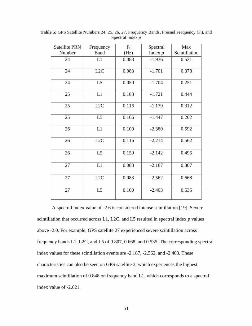
51
Table 5: GPS Satellite Numbers 24, 25, 26, 27, Frequency Bands, Fresnel Frequency (Ff), and
Spectral Index p
A spectral index value of -2.6 is considered intense scintillation [19]. Severe
scintillation that occurred across L1, L2C, and L5 resulted in spectral index p values
above -2.0. For example, GPS satellite 27 experienced severe scintillation across
frequency bands L1, L2C, and L5 of 0.807, 0.668, and 0.535. The corresponding spectral
index values for these scintillation events are -2.187, -2.562, and -2.403. These
characteristics can also be seen on GPS satellite 3, which experiences the highest
maximum scintillation of 0.848 on frequency band L1, which corresponds to a spectral
index value of -2.621.
Satellite PRN
Number
Frequency
Band
Ff
(Hz)
Spectral
Index p
Max
Scintillation
24 L1 0.083 -1.936 0.521
24 L2C 0.083 -1.701 0.378
24 L5 0.050 -1.704 0.251
25 L1 0.183 -1.721 0.444
25 L2C 0.116 -1.179 0.312
25 L5 0.166 -1.447 0.202
26 L1 0.100 -2.380 0.592
26 L2C 0.116 -2.214 0.562
26 L5 0.150 -2.142 0.496
27 L1 0.083 -2.187 0.807
27 L2C 0.083 -2.562 0.668
27 L5 0.100 -2.403 0.535

52
Figure 30: Power spectral density graph amplitude in (blue) for frequency L1, L2C, L5
The power spectral density of amplitude for GPS satellite 9 is shown in Figure
30. The Fresnel frequency is estimated at the roll off, which is indicated by the upper
point in the graph. The second point is the point where the signal beings to degrade, at the
noise floor. A line is drawn from the Fresnel frequency to the low cut of frequency, at the

53
start of the noise floor. A linear interpolation is used to estimate spectral index p of the
lines for each frequency band L1, L2C, and L5.
Figure 31: Signal power in dB for GLONASS satellites 1, 2, 3, and 4 G1 (Red) and G2 (Black)
GLONASS satellites 1, 2, 3, 4 are used to compare the signal power transmitted
on frequency bands G1 and G2. For the GLONASS plots, G1 is colored in red and G2 is
colored in black. Power spectral density of amplitude is used to compute spectral index p
across G1 and G2, to determine scintillation intensity. As shown in Figure 31, G1 tends
to fade less than G2. G1 maintains an average intensity of 100.95 dB and G2 maintains
average intensity levels of 98.11 dB. Like GPS L1 and L2, GLONASS G1 and G2 have
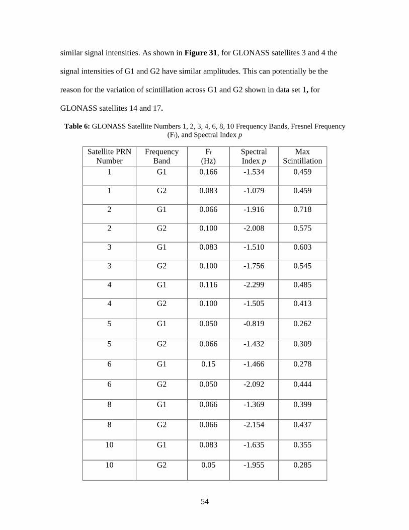
54
similar signal intensities. As shown in Figure 31, for GLONASS satellites 3 and 4 the
signal intensities of G1 and G2 have similar amplitudes. This can potentially be the
reason for the variation of scintillation across G1 and G2 shown in data set 1, for
GLONASS satellites 14 and 17.
Table 6: GLONASS Satellite Numbers 1, 2, 3, 4, 6, 8, 10 Frequency Bands, Fresnel Frequency
(Ff), and Spectral Index p
Satellite PRN
Number
Frequency
Band
Ff
(Hz)
Spectral
Index p
Max
Scintillation
1 G1 0.166 -1.534 0.459
1 G2 0.083 -1.079 0.459
2 G1 0.066 -1.916 0.718
2 G2 0.100 -2.008 0.575
3 G1 0.083 -1.510 0.603
3 G2 0.100 -1.756 0.545
4 G1 0.116 -2.299 0.485
4 G2 0.100 -1.505 0.413
5 G1 0.050 -0.819 0.262
5 G2 0.066 -1.432 0.309
6 G1 0.15 -1.466 0.278
6 G2 0.050 -2.092 0.444
8 G1 0.066 -1.369 0.399
8 G2 0.066 -2.154 0.437
10 G1 0.083 -1.635 0.355
10 G2 0.05 -1.955 0.285
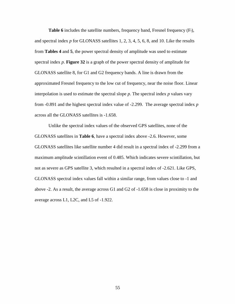
55
Table 6 includes the satellite numbers, frequency band, Fresnel frequency (Ff),
and spectral index p for GLONASS satellites 1, 2, 3, 4, 5, 6, 8, and 10. Like the results
from Tables 4 and 5, the power spectral density of amplitude was used to estimate
spectral index p. Figure 32 is a graph of the power spectral density of amplitude for
GLONASS satellite 8, for G1 and G2 frequency bands. A line is drawn from the
approximated Fresnel frequency to the low cut of frequency, near the noise floor. Linear
interpolation is used to estimate the spectral slope p. The spectral index p values vary
from -0.891 and the highest spectral index value of -2.299. The average spectral index p
across all the GLONASS satellites is -1.658.
Unlike the spectral index values of the observed GPS satellites, none of the
GLONASS satellites in Table 6, have a spectral index above -2.6. However, some
GLONASS satellites like satellite number 4 did result in a spectral index of -2.299 from a
maximum amplitude scintillation event of 0.485. Which indicates severe scintillation, but
not as severe as GPS satellite 3, which resulted in a spectral index of -2.621. Like GPS,
GLONASS spectral index values fall within a similar range, from values close to -1 and
above -2. As a result, the average across G1 and G2 of -1.658 is close in proximity to the
average across L1, L2C, and L5 of -1.922.

56
Figure 32: Power spectral density graph of amplitude in (blue) for frequency band G1 and G2
Figure 33 includes plots of signal power for Galileo satellites 11, 12, and 22
frequency bands E1 (red), E5A (black), E5B (blue). E5B maintains a higher signal power
than signals transmitted on E1 and E5A. E5B has an average signal power of 111 dB.
Frequency bands E1 and E5A have an average signal power of 102.82 and 101.84 dB.
Frequency band E1 is slightly higher than E5A for both satellites 11 and 22, but the
signal power does intersect and fluctuate between them. Like GPS L1, L2, and
GLONASS G1, G2, Galileo E1 and E5A have similar signal strength. As shown in
Figure 33, the signal strength of E1 and E5A are similar for Galileo satellite 12, in which
they overlap.
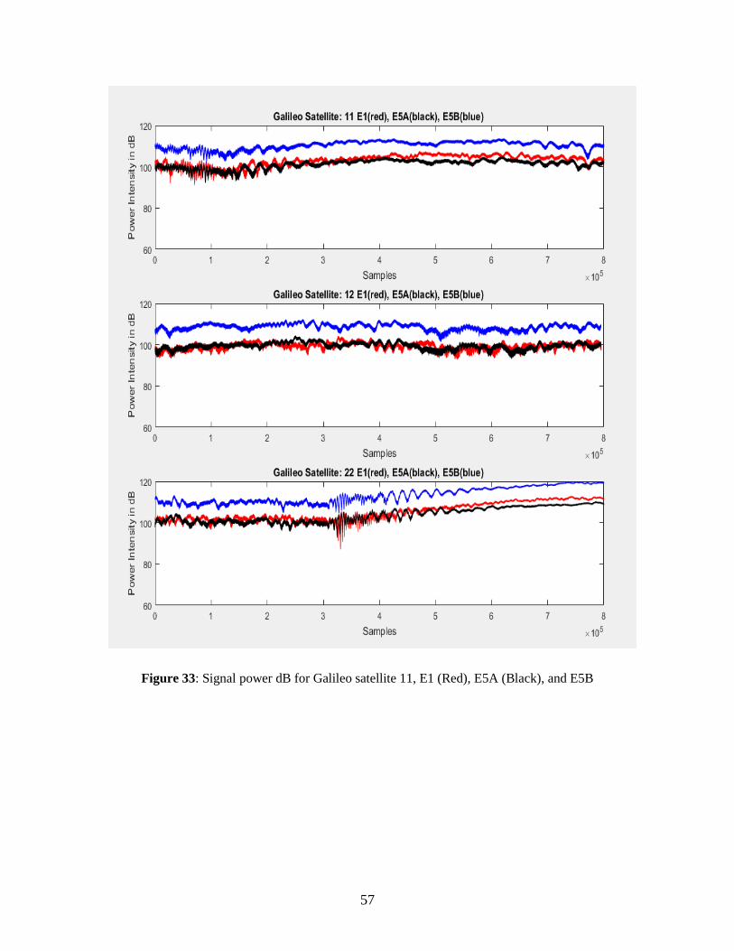
57
Figure 33: Signal power dB for Galileo satellite 11, E1 (Red), E5A (Black), and E5B
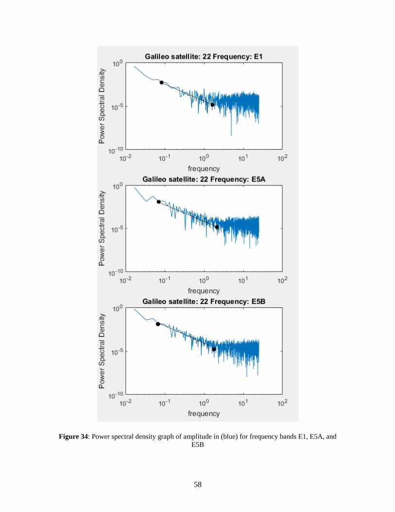
58
Figure 34: Power spectral density graph of amplitude in (blue) for frequency bands E1, E5A, and
E5B
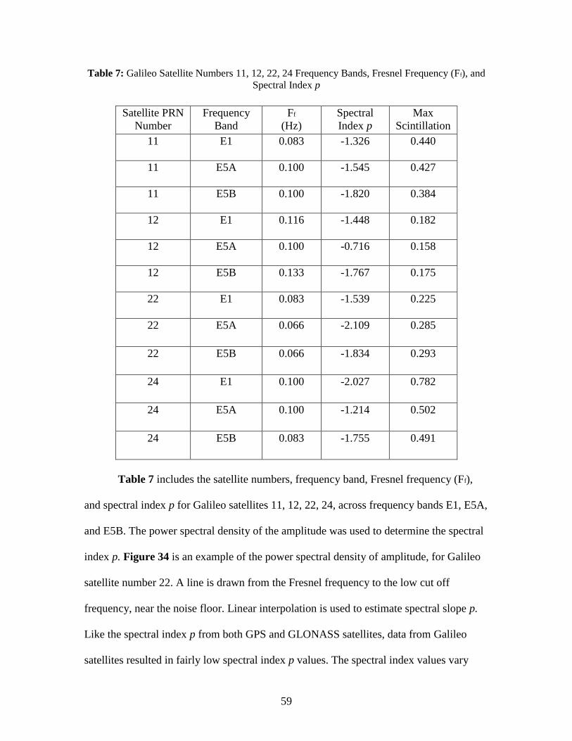
59
Table 7: Galileo Satellite Numbers 11, 12, 22, 24 Frequency Bands, Fresnel Frequency (Ff), and
Spectral Index p
Table 7 includes the satellite numbers, frequency band, Fresnel frequency (Ff),
and spectral index p for Galileo satellites 11, 12, 22, 24, across frequency bands E1, E5A,
and E5B. The power spectral density of the amplitude was used to determine the spectral
index p. Figure 34 is an example of the power spectral density of amplitude, for Galileo
satellite number 22. A line is drawn from the Fresnel frequency to the low cut off
frequency, near the noise floor. Linear interpolation is used to estimate spectral slope p.
Like the spectral index p from both GPS and GLONASS satellites, data from Galileo
satellites resulted in fairly low spectral index p values. The spectral index values vary
Satellite PRN
Number
Frequency
Band
Ff
(Hz)
Spectral
Index p
Max
Scintillation
11 E1 0.083 -1.326 0.440
11 E5A 0.100 -1.545 0.427
11 E5B 0.100 -1.820 0.384
12 E1 0.116 -1.448 0.182
12 E5A 0.100 -0.716 0.158
12 E5B 0.133 -1.767 0.175
22 E1 0.083 -1.539 0.225
22 E5A 0.066 -2.109 0.285
22 E5B 0.066 -1.834 0.293
24 E1 0.100 -2.027 0.782
24 E5A 0.100 -1.214 0.502
24 E5B 0.083 -1.755 0.491

60
from -0.710 to as high as -2.109. The average spectral index across the Galileo satellites
is -1.575.
Like GPS and GLONASS, Galileo spectral index p values are close to -1 and -2.
The highest spectral index value of -2.109 was experienced by satellite 22 on frequency
band E5A. The average spectral index across E1, E5A, and E5B is -1.575, which is close
in proximity to the averages of GPS -1.922 and GLONASS -1.658. The average across
these constellations aren’t near a spectral index p of -2.6, which indicates that the
scintillation events are fairly moderate.
4.3.2 Summary
The signal power graphs for GPS indicate that L5 fades less than both L1 and L2.
This also shows that the received signal strength of L5 is stronger than both L1 and L2.
This validates the previous results from data set 1, where L5 scintillated less than L1 and
L2. Previous studies at low latitudes indicates that lower frequency bands tend to fade
more than higher frequency bands [21], [22]. Results from this research indicate that at
mid-latitudes lower frequency band L5 fades less than higher frequency bands L1 and L2.
However, like the previous research, L1 did fade less than L2 [21].
G1 fades less than G2, but there are periods of time in which G2 fades less than
G1, since both frequency bands have similar intensities. E5B has an average signal power
of 111 dB, which is higher than the average signal power of E1 at 102.82 dB and E5A at
101.84 dB. As a result, E5B faded less than both E1 and E5A. Like G1 and G2, E1 and
E5A have similar signal intensities, which causes a variation in fade across both
frequency bands. Sometimes E1 may fade less than E5A, but other times E5A may fade
less than E1.
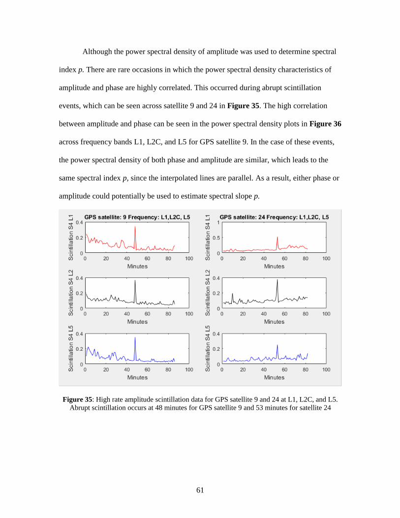
61
Although the power spectral density of amplitude was used to determine spectral
index p. There are rare occasions in which the power spectral density characteristics of
amplitude and phase are highly correlated. This occurred during abrupt scintillation
events, which can be seen across satellite 9 and 24 in Figure 35. The high correlation
between amplitude and phase can be seen in the power spectral density plots in Figure 36
across frequency bands L1, L2C, and L5 for GPS satellite 9. In the case of these events,
the power spectral density of both phase and amplitude are similar, which leads to the
same spectral index p, since the interpolated lines are parallel. As a result, either phase or
amplitude could potentially be used to estimate spectral slope p.
Figure 35: High rate amplitude scintillation data for GPS satellite 9 and 24 at L1, L2C, and L5.
Abrupt scintillation occurs at 48 minutes for GPS satellite 9 and 53 minutes for satellite 24
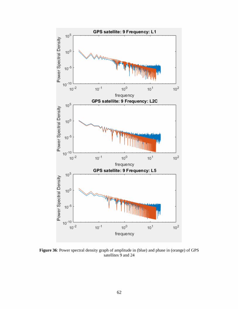
62
Figure 36: Power spectral density graph of amplitude in (blue) and phase in (orange) of GPS
satellites 9 and 24
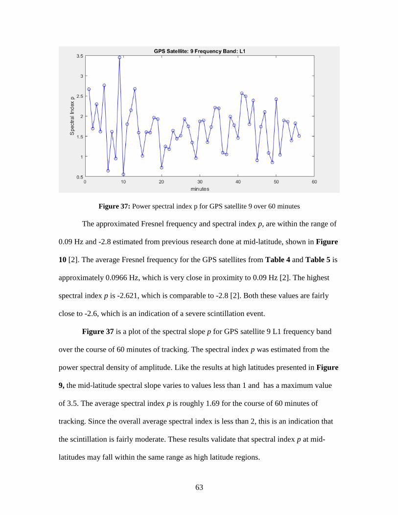
63
Figure 37: Power spectral index p for GPS satellite 9 over 60 minutes
The approximated Fresnel frequency and spectral index p, are within the range of
0.09 Hz and -2.8 estimated from previous research done at mid-latitude, shown in Figure
10 [2]. The average Fresnel frequency for the GPS satellites from Table 4 and Table 5 is
approximately 0.0966 Hz, which is very close in proximity to 0.09 Hz [2]. The highest
spectral index p is -2.621, which is comparable to -2.8 [2]. Both these values are fairly
close to -2.6, which is an indication of a severe scintillation event.
Figure 37 is a plot of the spectral slope p for GPS satellite 9 L1 frequency band
over the course of 60 minutes of tracking. The spectral index p was estimated from the
power spectral density of amplitude. Like the results at high latitudes presented in Figure
9, the mid-latitude spectral slope varies to values less than 1 and has a maximum value
of 3.5. The average spectral index p is roughly 1.69 for the course of 60 minutes of
tracking. Since the overall average spectral index is less than 2, this is an indication that
the scintillation is fairly moderate. These results validate that spectral index p at mid-
latitudes may fall within the same range as high latitude regions.

64
The average spectral index across L1, L2C, L5, G1, G2, E1, E5A, and E5B
frequency bands is roughly -1.764 and the average. Since the average of the power
spectral density across all the satellites isn’t near the value of -2.6, it can be interpreted
that scintillation is fairly moderate for these observations.
4.4 Data Set 3 Presentation
Data set 3 was collected for 11 days, from August 4th to August 15th, 2016 This
data set was used to test if previous assumptions would hold true for longer periods of
time. Data set 3 was collected during moderate space weather conditions with low Kp
index values. The Kp index values shown in Figure 38, maintain values from 2 to 4,
which indicate moderate activity.
Figure 38: Range of Kp index values for data set 3, which range from Kp of 2 to 4 [25]
Low rate scintillation was collected for data set 3. Histogram distributions of
scintillation density are plotted across GPS L1, L2, L5, GLONASS, G1, G2, and Galileo
E1, E5A, E5B, in order to determine which frequency bands had the best overall

65
performance, over the 11-day period. Since data is collected over a longer period of time,
it can better validate results from data set 1 and data set 2.
4.4.1 Scintillation Analysis
The eight GPS satellites that transmit L1, L2, and L5 are used to compare the
performance of L1, L2, and L5. Again, the scintillation data is plotted for satellites above
15 degrees, in order to mitigate multipath effects. Histogram distributions were plotted
for GPS satellites 6, 8, 9, 26, 27, and 30. It can be seen from Figure 39 and Figure 40,
that L5 scintillated less than both L1 and L2 for the 11-day period. Signals transmitted
on frequency band L1 scintillated less than L2, over the 11-day period. Compared to L1
and L5, L2 had the worst performance. These results validate the previous assumptions
made, that at mid-latitudes L5 performs better than L1 and L2, from data set 1 and 2.
Figure 39: Histogram distribution of GPS satellites 26 (top) and 30 (bottom) L1, L2, L5 over 11-
day period

66
Figure 40: 11-day period and histogram distribution of GPS satellites 6 and 8 (top) and 9 and 27
(bottom) L1, L2, L5 over 11-day period
GLONASS satellites 2 and 3 scintillation distributions across G1 and G2 are
shown in Figure 41. Like data set 1, scintillation across GLONASS satellites in data set 3
show characteristic differences between G1 and G2. For example, G1 scintillates less
than G2 for GLONASS satellite number 3. However, for GLONASS satellite 2 G1
scintillates less than G2 at the start of the distribution, but as the distribution continues
G2 scintillates less than G1. As previously mentioned, the discrepancies in scintillation
could’ve been caused by FDMA, since signal transmitted on G1 and G2 frequency bands
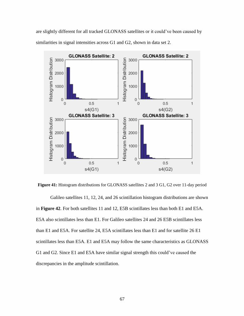
67
are slightly different for all tracked GLONASS satellites or it could’ve been caused by
similarities in signal intensities across G1 and G2, shown in data set 2.
Figure 41: Histogram distributions for GLONASS satellites 2 and 3 G1, G2 over 11-day period
Galileo satellites 11, 12, 24, and 26 scintillation histogram distributions are shown
in Figure 42. For both satellites 11 and 12, E5B scintillates less than both E1 and E5A.
E5A also scintillates less than E1. For Galileo satellites 24 and 26 E5B scintillates less
than E1 and E5A. For satellite 24, E5A scintillates less than E1 and for satellite 26 E1
scintillates less than E5A. E1 and E5A may follow the same characteristics as GLONASS
G1 and G2. Since E1 and E5A have similar signal strength this could’ve caused the
discrepancies in the amplitude scintillation.

68
Figure 42: Histogram distributions for Galileo satellites 11 and 12 (top) and Galileo 24 and 26
(bottom) E1, E5A, and E5B over 11-day period
4.4.2 Statistical and Cross Correlation Analysis
Statistical Distribution
A statistical analysis is done across GPS L1, L2, L5, GLONASS G1, G2, and
Galileo E1, E5A, E5B bands to measure the probability of phase and amplitude
scintillation occurring at specific ranges. For amplitude scintillation, the range is taken by
0.1 increments from 0 to 1 and for phase scintillation the range is taken by 10 degree
increments from 0 to 100 degrees. The purpose of these measurements is to compare the
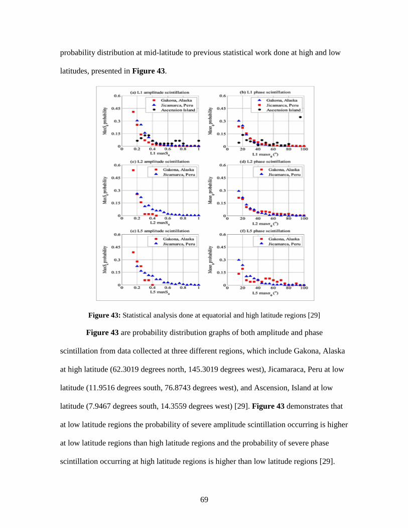
69
probability distribution at mid-latitude to previous statistical work done at high and low
latitudes, presented in Figure 43.
Figure 43: Statistical analysis done at equatorial and high latitude regions [29]
Figure 43 are probability distribution graphs of both amplitude and phase
scintillation from data collected at three different regions, which include Gakona, Alaska
at high latitude (62.3019 degrees north, 145.3019 degrees west), Jicamaraca, Peru at low
latitude (11.9516 degrees south, 76.8743 degrees west), and Ascension, Island at low
latitude (7.9467 degrees south, 14.3559 degrees west) [29]. Figure 43 demonstrates that
at low latitude regions the probability of severe amplitude scintillation occurring is higher
at low latitude regions than high latitude regions and the probability of severe phase
scintillation occurring at high latitude regions is higher than low latitude regions [29].

70
The research also showed that scintillation across L2 and L5 are more severe than L1 in
both high latitude and low latitude regions [29].
Figure 44: Probability distribution of amplitude and phase scintillation across GPS L1, L2, L5 at
mid-latitude for 11 – day period
As shown in Figure 44, L5 has the highest probability of 72% of falling within
the lowest scintillation region from 0 to 0.1. L1 and L2 have lower probabilities of
57.94% and 53.6% of falling within the lowest scintillation range. Compared to the
amplitude scintillation probability distributions from high and low latitude regions in
Figure 43, it is clear that at mid-latitudes the majority of amplitude scintillation events
fall within the lowest range of 0 to 0.1 and are less severe. The phase probability
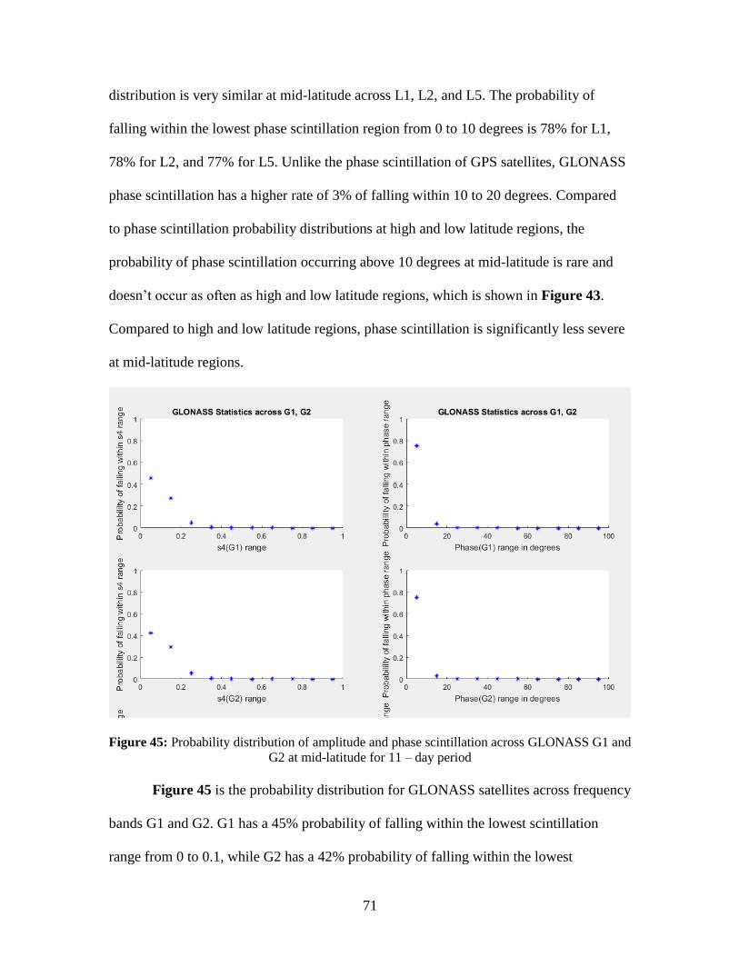
71
distribution is very similar at mid-latitude across L1, L2, and L5. The probability of
falling within the lowest phase scintillation region from 0 to 10 degrees is 78% for L1,
78% for L2, and 77% for L5. Unlike the phase scintillation of GPS satellites, GLONASS
phase scintillation has a higher rate of 3% of falling within 10 to 20 degrees. Compared
to phase scintillation probability distributions at high and low latitude regions, the
probability of phase scintillation occurring above 10 degrees at mid-latitude is rare and
doesn’t occur as often as high and low latitude regions, which is shown in Figure 43.
Compared to high and low latitude regions, phase scintillation is significantly less severe
at mid-latitude regions.
Figure 45: Probability distribution of amplitude and phase scintillation across GLONASS G1 and
G2 at mid-latitude for 11 – day period
Figure 45 is the probability distribution for GLONASS satellites across frequency
bands G1 and G2. G1 has a 45% probability of falling within the lowest scintillation
range from 0 to 0.1, while G2 has a 42% probability of falling within the lowest
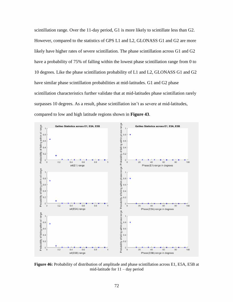
72
scintillation range. Over the 11-day period, G1 is more likely to scintillate less than G2.
However, compared to the statistics of GPS L1 and L2, GLONASS G1 and G2 are more
likely have higher rates of severe scintillation. The phase scintillation across G1 and G2
have a probability of 75% of falling within the lowest phase scintillation range from 0 to
10 degrees. Like the phase scintillation probability of L1 and L2, GLONASS G1 and G2
have similar phase scintillation probabilities at mid-latitudes. G1 and G2 phase
scintillation characteristics further validate that at mid-latitudes phase scintillation rarely
surpasses 10 degrees. As a result, phase scintillation isn’t as severe at mid-latitudes,
compared to low and high latitude regions shown in Figure 43.
Figure 46: Probability of distribution of amplitude and phase scintillation across E1, E5A, E5B at
mid-latitude for 11 – day period

73
Figure 46 is the probability distribution for Galileo satellites across frequency
bands E1, E5A, and E5B. The probability of falling within the lowest scintillation range
from 0 to 0.1 is 65% for E1, 71% for E5A, and 74% for E5B. E5B is more likely to
scintillate less than both E1 and E5A. E5A is more likely to scintillate less than E1. Like
GPS and GLONASS, Galileo phase scintillation have similar probabilities of falling
within the lowest phase scintillation range. E1, E5A, and E5B all have a 79% chance of
falling within 0 to 10 degrees. This further proves the point that phase scintillation isn’t
as severe in mid-latitudes, compared to low and high latitudes presented in Figure 43.
Frequency Band Cross Correlation of Amplitude and Phase scintillation
Both amplitude and phase scintillation cross correlations across the frequency
bands are plotted. For example, for a plot of amplitude scintillation across (L1 vs. L2), if
the slope leans towards the L1 axis then the L1 scintillation is more severe than L2. If the
slope of the line is close to the value of 1, then this means that the L1 and L2
scintillations are comparable.
Figure 47 are linear fit graphs for GPS satellites 1 and 25 across L1, L2, L5 for
both amplitude and phase scintillation. Both amplitude and phase scintillation are plotted
with respect to (L1 vs. L2), (L1 vs. L5), and (L2 vs. L5). Linear curves are fitted over the
data points and the slopes are listed for each line. For the fitted curves over (L1 vs. L2)
and (L1 vs. L5), the slopes are greater than one for both amplitude and phase scintillation.
Since the slopes are greater than one, this means that L2 and L5 frequency bands resulted
in greater scintillation than L1. The slopes across (L2 vs. L5) are closer to 1, which is an
indication of high correlation between both the amplitude and phase scintillation

74
characteristics across L2 and L5. The results are similar across data taken from high
latitude in Gakona, Alaska and low latitude in Jicamarca, Peru.
Figure 47: Linear fit curves across GPS L1, L2, L5 amplitude and phase scintillation for
satellites 1 and 25 [29]
Figure 48 includes the plots and lists the slopes of the linear fit curves of data
collected at mid-latitude over the 11-day period, for both amplitude and phase
scintillation, for GPS satellites 1 and 25. The slope values across (L1 vs. L2) are fairly
close to one for both amplitude and phase scintillation, which indicates that the
scintillation events across L1 and L2 have similar characteristics. This also agrees with
the statistics shown in Figure 44, which shows that L1 and L2 have similar probabilities
of falling within the lowest range of amplitude and phase scintillation. However, L1 does
slightly do better than L2, with a 4% greater chance of falling within the lowest
75
amplitude scintillation range. Since the phase scintillation has a higher correlation than
amplitude scintillation, the probability of both L1 and L2 have an equivalent probability
of 78% of falling within the lowest phase scintillation range.
(L1 vs. L5) have slopes that lean more towards the L1 axis for amplitude
scintillation and slope values closer to one for phase scintillation. The correlation of
phase scintillation is higher than amplitude scintillation. The correlation characteristics
can be seen in the probability distribution in Figure 44, which shows that L5 has a 14%
greater chance of falling within the lowest amplitude scintillation range compared to L5.
Since the phase scintillation has a high correlation, the probability of falling within the
lowest phase range is only 1% difference between L1 and L5.
(L2 vs. L5) have slopes that lean more towards L2 than L5 for amplitude
scintillation and have slopes closer to one for phase scintillation. The correlation
characteristics can be seen in the probability distribution in Figure 45, which shows that
L5 has an 18% greater chance of falling within lower amplitude scintillation ranges.
Since phase has a greater correlation than amplitude, there is only a 1% difference
between L2 and L5 of falling within the lowest phase scintillation range. This further
validates the point that L5 has less severe amplitude scintillation, compared to L1 and L2
at mid-latitude.

76
(L1 vs. L2) R = 0.8949
(L1 vs. L2) R = 0.9645
(L1 vs. L5) R = 0.5107
(L1 vs. L5) R = 0.6959
(L2 vs. L5) R = 0.5416
(L2 vs. L5) R = 0.7143
(L1 vs. L2) R = 0.8706
(L1 vs. L2) R = 0.9637
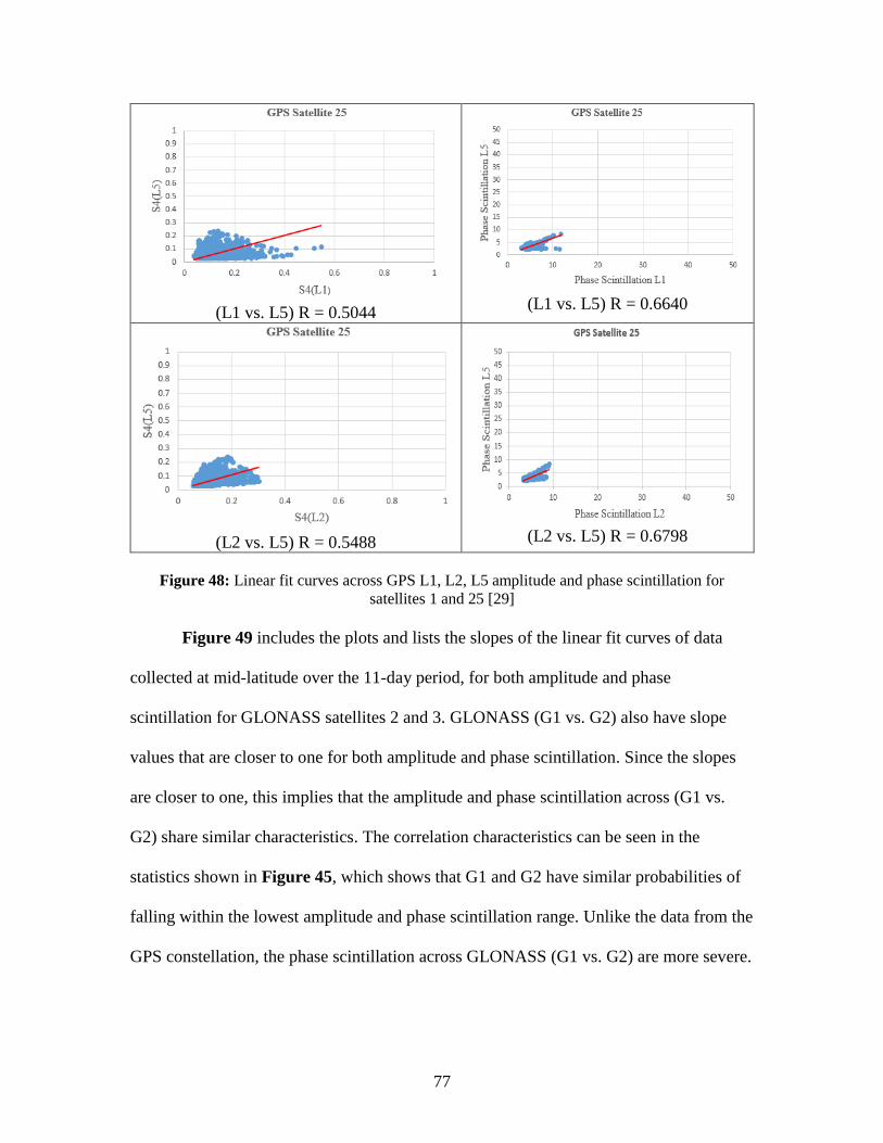
77
Figure 48: Linear fit curves across GPS L1, L2, L5 amplitude and phase scintillation for
satellites 1 and 25 [29]
Figure 49 includes the plots and lists the slopes of the linear fit curves of data
collected at mid-latitude over the 11-day period, for both amplitude and phase
scintillation for GLONASS satellites 2 and 3. GLONASS (G1 vs. G2) also have slope
values that are closer to one for both amplitude and phase scintillation. Since the slopes
are closer to one, this implies that the amplitude and phase scintillation across (G1 vs.
G2) share similar characteristics. The correlation characteristics can be seen in the
statistics shown in Figure 45, which shows that G1 and G2 have similar probabilities of
falling within the lowest amplitude and phase scintillation range. Unlike the data from the
GPS constellation, the phase scintillation across GLONASS (G1 vs. G2) are more severe.
(L1 vs. L5) R = 0.5044
(L1 vs. L5) R = 0.6640
(L2 vs. L5) R = 0.5488
(L2 vs. L5) R = 0.6798

78
It can be seen from the plot that GLONASS satellite 2 have phase scintillation above 20
degrees and for satellite 3 above 40 degrees.
(G1 vs. G2) R = 0.8146
(G1 vs. G2) R = 0.8019
(G1 vs. G2) R = 0.855
(G1 vs. G2) R = 0.8147
Figure 49: Linear fit curves across GLONASS amplitude and phase scintillation for satellites 2
and 3
Figure 50 includes the plots and lists the slopes of the linear fit curves of data
collected at mid-latitude over the 11-day period, for both amplitude and phase
scintillation across Galileo satellites 24 and 26. (E1 vs. E5A) have slopes that are fairly
close to one for both amplitude and phase. However, the slope across the phase is closer
to one than the slope of the amplitude. This means that there is a higher correlation for
phase than amplitude. The correlation characteristics can be seen in the statistical
distribution shown Figure 46, which shows that E5A has a 6% greater chance of falling

79
within the lowest amplitude scintillation range, compared to E1. For phase both E1 and
E5A have a 79% equivalent probability of falling within the lowest phase range.
(E1 vs. E5B) have slopes that lean towards E1 for amplitude and slope values that
are closer to one for phase. This indicates that E1 has more severe amplitude scintillation,
compared to E5A. For phase scintillation E1 and E5B have higher correlation
characteristics, compared to amplitude scintillation. The correlation characteristics can be
seen in the statistical distribution in Figure 46, which shows that E5B has an 8% greater
chance of falling within the lowest amplitude scintillation range than E5B. The statistical
analysis also shows that E1 and E5B have an equivalent probability of falling within the
lowest phase scintillation range of 79%.
(E5A vs. E5B) plots have slopes that are fairly close to one for both amplitude
and phase scintillation. This means that the scintillation characteristics of amplitude and
phase are similar across E5A and E5B. However, it can be seen from the correlation
characteristics shown in the probability distribution shown in Figure 46, that E5B has a
3% greater chance at falling within the lowest amplitude scintillation range, compared to
E5A. E5A and E5B have both have equivalent probability of falling within the lowest
scintillation range of 79%. This indicates that the phase scintillation has a high
correlation across both frequency bands. Overall, these results show that E5B
outperforms both E1 and E5A. Like GLONASS, Galileo signals have phase scintillation
that can occur above 40 degrees.
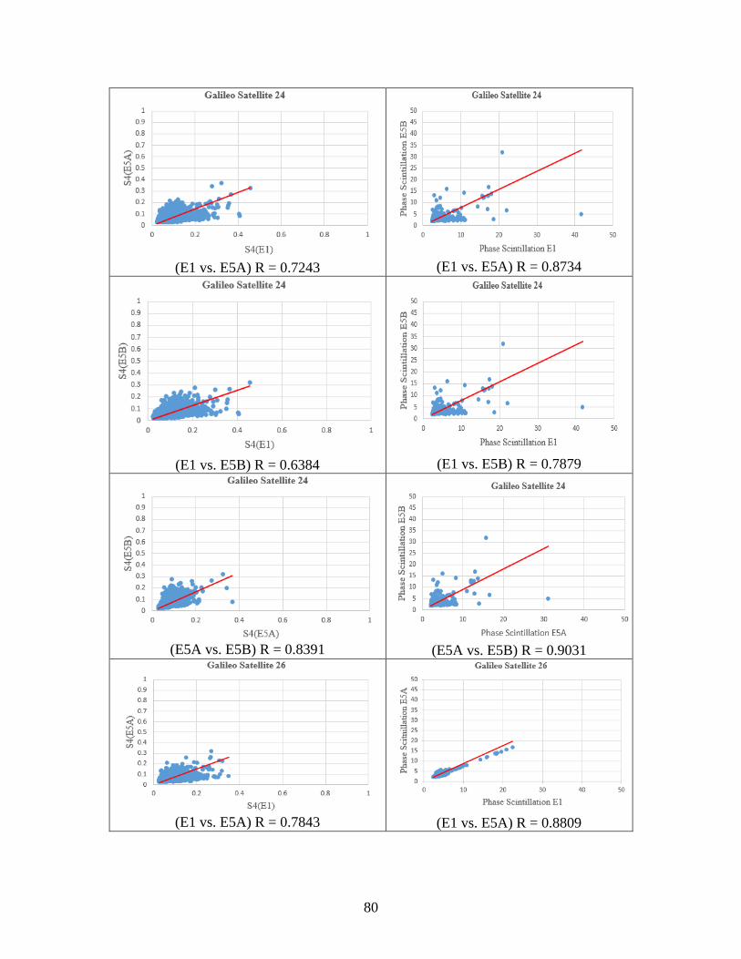
80
(E1 vs. E5A) R = 0.7243
(E1 vs. E5A) R = 0.8734
(E1 vs. E5B) R = 0.6384
(E1 vs. E5B) R = 0.7879
(E5A vs. E5B) R = 0.8391
(E5A vs. E5B) R = 0.9031
(E1 vs. E5A) R = 0.7843
(E1 vs. E5A) R = 0.8809
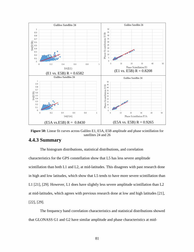
81
Figure 50: Linear fit curves across Galileo E1, E5A, E5B amplitude and phase scintillation for
satellites 24 and 26
4.4.3 Summary
The histogram distributions, statistical distributions, and correlation
characteristics for the GPS constellation show that L5 has less severe amplitude
scintillation than both L1 and L2, at mid-latitudes. This disagrees with past research done
in high and low latitudes, which show that L5 tends to have more severe scintillation than
L1 [21], [29]. However, L1 does have slightly less severe amplitude scintillation than L2
at mid-latitudes, which agrees with previous research done at low and high latitudes [21],
[22], [29].
The frequency band correlation characteristics and statistical distributions showed
that GLONASS G1 and G2 have similar amplitude and phase characteristics at mid-
(E1 vs. E5B) R = 0.6582
(E1 vs. E5B) R = 0.8208
(E5A vs.E5B) R = 0.8430
(E5A vs. E5B) R = 0.9265

82
latitude. The frequency band correlation across both amplitude and phase are close to
one, which indicates that the scintillation characteristics are similar. The similarities can
also be seen in the statistical analysis, which shows that both G1 and G2 have similar
probability distributions. However, G1 does have a slightly greater probability of 3% of
falling within the lowest amplitude scintillation range.
The correlation across E1 and E5A is higher for phase than amplitude. Both
frequency bands had similar phase scintillation characteristics. E5A has less severe
amplitude scintillation than E1. The correlation across E1 and E5B showed higher
similarities across phase scintillation than amplitude scintillation. E5B had less severe
amplitude scintillation than E1. The correlation of amplitude and phase scintillation
across E5A and E5B is high, since the slopes across these frequency bands are also
relatively close to the value of one. However, E5B has slightly less severe scintillation
than EA. These results are interesting since it was shown previously in data set 2, that
E5B has a signal power that is on average roughly 9 dB higher than E5A. This proves
that even though a signal has a greater receive power, it doesn’t necessarily mean that it
will fade less than signals with less receive power. Other factors, such as signal wave
length, may play a role on the severity of scintillation.
Based on the results from the probability distribution, the phase scintillation
across GPS, GLONASS, and Galileo constellations rarely fall above 10 degrees. Based
on the amplitude scintillation probability distributions both GPS and Galileo have a
higher probability of having less severe amplitude and phase scintillation compared to
GLONASS. At mid-latitude GLONASS tends to have the worst performance, having
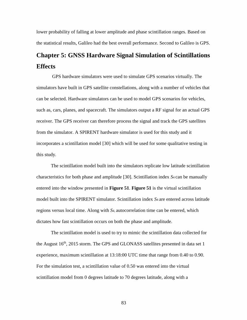
83
lower probability of falling at lower amplitude and phase scintillation ranges. Based on
the statistical results, Galileo had the best overall performance. Second to Galileo is GPS.
Chapter 5: GNSS Hardware Signal Simulation of Scintillations
Effects
GPS hardware simulators were used to simulate GPS scenarios virtually. The
simulators have built in GPS satellite constellations, along with a number of vehicles that
can be selected. Hardware simulators can be used to model GPS scenarios for vehicles,
such as, cars, planes, and spacecraft. The simulators output a RF signal for an actual GPS
receiver. The GPS receiver can therefore process the signal and track the GPS satellites
from the simulator. A SPIRENT hardware simulator is used for this study and it
incorporates a scintillation model [30] which will be used for some qualitative testing in
this study.
The scintillation model built into the simulators replicate low latitude scintillation
characteristics for both phase and amplitude [30]. Scintillation index S4 can be manually
entered into the window presented in Figure 51. Figure 51 is the virtual scintillation
model built into the SPIRENT simulator. Scintillation index S4 are entered across latitude
regions versus local time. Along with S4, autocorrelation time can be entered, which
dictates how fast scintillation occurs on both the phase and amplitude.
The scintillation model is used to try to mimic the scintillation data collected for
the August 16th, 2015 storm. The GPS and GLONASS satellites presented in data set 1
experience, maximum scintillation at 13:18:00 UTC time that range from 0.40 to 0.90.
For the simulation test, a scintillation value of 0.50 was entered into the virtual
scintillation model from 0 degrees latitude to 70 degrees latitude, along with a
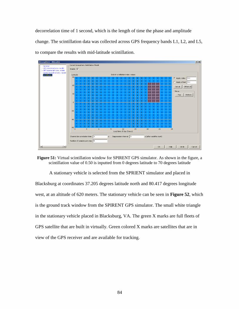
84
decorrelation time of 1 second, which is the length of time the phase and amplitude
change. The scintillation data was collected across GPS frequency bands L1, L2, and L5,
to compare the results with mid-latitude scintillation.
Figure 51: Virtual scintillation window for SPIRENT GPS simulator. As shown in the figure, a
scintillation value of 0.50 is inputted from 0 degrees latitude to 70 degrees latitude
A stationary vehicle is selected from the SPRIENT simulator and placed in
Blacksburg at coordinates 37.205 degrees latitude north and 80.417 degrees longitude
west, at an altitude of 620 meters. The stationary vehicle can be seen in Figure 52, which
is the ground track window from the SPIRENT GPS simulator. The small white triangle
in the stationary vehicle placed in Blacksburg, VA. The green X marks are full fleets of
GPS satellite that are built in virtually. Green colored X marks are satellites that are in
view of the GPS receiver and are available for tracking.

85
Figure 52: Ground track window from GPS simulator. The white triangle is the stationary
vehicle placed in Blacksburg, VA. X marks are GPS satellites that are built in virtually in the
GPS simulator
Data from this simulation was collected for about 40 minutes. Data from GPS
satellites 1, 4, 7, 20, and 23 are used to observe the performance of frequency bands L1,
L2, and L5. Figure 53 are scintillation graphs of satellite 1, 4, 7, and 20, for frequency
bands L1, L2, and L5. For GPS satellite 1, L1 is tracked for about 30 minutes, but L2 and
L5 lose lock within the first 3 minutes of tracking. This validates previous research done
at low latitudes, which shows that L1 tends to fade less than L2 and L5. However, in the
case of satellite 4, both L1 and L5 are tracked for 38 minutes and L2 loses track within
the first 6 minutes of tracking and L5 scintillates less than L2 and L1. This disagrees with
the idea that lower frequencies tend to do better than higher frequencies and agrees with
the analysis done on mid-latitude scintillation for this research, which showed higher
signal strengths on L5.
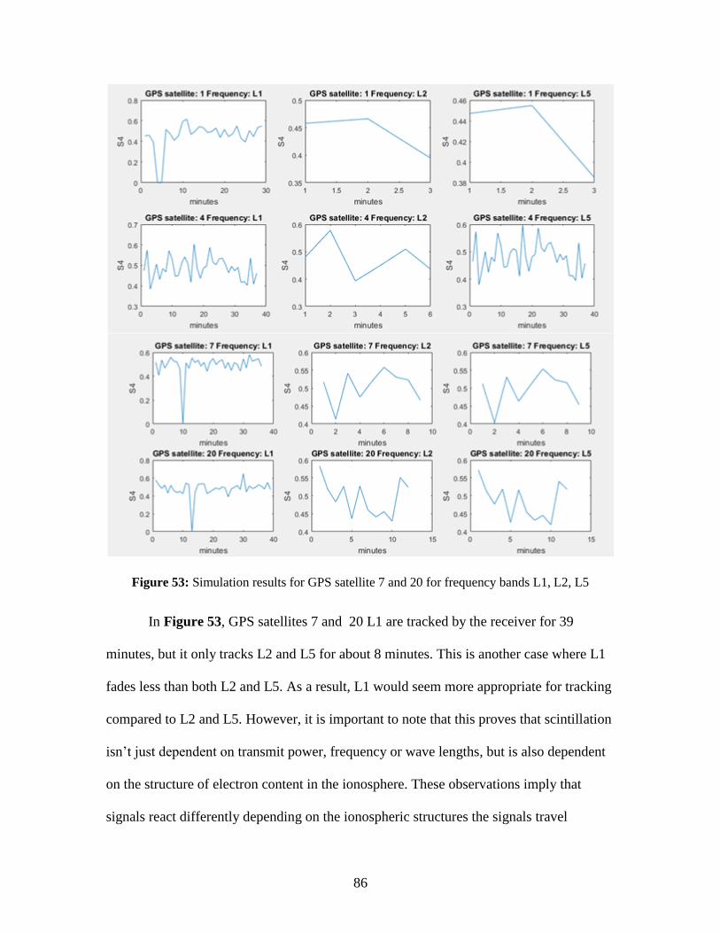
86
Figure 53: Simulation results for GPS satellite 7 and 20 for frequency bands L1, L2, L5
In Figure 53, GPS satellites 7 and 20 L1 are tracked by the receiver for 39
minutes, but it only tracks L2 and L5 for about 8 minutes. This is another case where L1
fades less than both L2 and L5. As a result, L1 would seem more appropriate for tracking
compared to L2 and L5. However, it is important to note that this proves that scintillation
isn’t just dependent on transmit power, frequency or wave lengths, but is also dependent
on the structure of electron content in the ionosphere. These observations imply that
signals react differently depending on the ionospheric structures the signals travel
87
through. Even within a simulation environment, discrepancies appear across the
frequency bands.
Chapter 6 Conclusion and Future Work
The purpose of this study was to consider if GNSS scintillation could be
consequential in mid-latitude regions and compare scintillation at mid-latitude to
pervious research done in low latitude, mid-latitude, and high latitude regions. This study
was also used to consider which GNSS frequency bands are more favorable at mid-
latitudes and how they compare to high and low latitudes. Data sets collected over
different time periods were used for this study. However, it is important to note that the
data is taken at mid-latitude at only one location, Blacksburg, VA, at coordinates 37.205
degrees latitude north and 80.417 degrees longitude west. As a result, this study is limited
and further investigation at other mid-latitude locations needs to be done to further
validate the results found in this research.
Shown in data set 1, mid-latitude scintillation could potentially be just as severe
as low latitude regions, but for very short durations of time. Data set 1 was collected
during a small geomagnetic storm. In data set 1, satellites from the GPS, GLONASS, and
Galileo constellation all exhibited high scintillation for a short duration of time. As
shown in data set 1, some of these satellites experienced scintillation ranging from 0.8 to
0.9.
Based on all three data sets, GPS L5 had less amplitude and phase scintillation
than GPS frequency bands L1, at mid-latitude. Frequency band L5 had less severe
scintillation, during the small geomagnetic storm on August the 15th, 2015, which is
88
analyzed in data set 1. Satellites transmitting on L5 not only scintillated less, but also had
better overall carrier to noise ratio density.
As seen from the signal power plots in data set 2, GPS L5 has an average signal
power of 106.48 dB, while both L1 and L2 have signal intensities of 100.93 dB and
100.54 dB. On average L5 has roughly 6 dB more signal power than both L1 and L2.
Having higher transmit power could be a factor for having less scintillation and higher
carrier to noise ratio density.
Histogram, correlation, and statistical distributions done on Data set 3 showed
that L5 had less severe amplitude scintillation, compared to L1 and L2. The analysis also
showed that L1 had slightly less severe amplitude scintillation than L2. The probability
distributions also showed that the phase is fairly similar across all three frequency bands.
This further validates the point that phase scintillation isn’t as severe at mid-latitudes,
compared to amplitude scintillation.
The correlation analysis done on GLONASS satellites show that the slopes of (G1
vs. G2) are above 0.80 for both amplitude and phase scintillation, which means that the
scintillation characteristics across both frequency bands are fairly similar. The statistical
analysis also shows that G1 and G2 have relatively close probabilities of falling within
the lowest amplitude and phase scintillation range.
The probability distribution and cross correlation analysis done on Galileo show
that E5A is more likely have less severe amplitude scintillation than E1. The analysis also
show that E5B had less severe amplitude scintillation compared to E1. The cross
correlation analysis and statistical analysis done on E5A and E5B show that E5B has less
severe amplitude scintillation, compared to E5A. However, it is important to note that

89
E5A and E5B amplitude and phase scintillation have high correlation. Even though E5B
on average has a 9 dB higher signal power than E5A, both frequency bands still share
similar scintillation characteristics. This proves that transmit power is not the only
variable that plays a role on scintillation, but other factors like the ionospheric structure,
signal wave lengths, etc. may also be a factor in scintillation.
Aspects of these observations are in line with past observations at low latitudes,
but there are some aspects that are different. For mid-latitude, L5 outperforms both L1
and L2. L1 performs slightly better than L2. At low latitude L1 fades less than both L2
and L5 [21], [29]. As a result, further investigation was done using the low latitude
scintillation model built into SPIRENT GPS simulators. Based on the data plotted from
the simulation shown in Figure 53, L2 and L5 tend to fade more than L1 at low latitudes.
GPS satellites 1, 7, 20 all lose lock on L2 and L5, but not on L1. In the case of GPS
satellite 4, L1 and L5 were both tracked and L2 lost lock. L1 is continuously tracked
across all the satellites and is less likely to lose lock compared to L2 and L5. This shows
that at low latitudes, L1 outperforms L2 and L5. However, that is not the case at mid-
latitudes, where L5 scintillates less than both L1 and L2. For the GPS constellation, the
study done at mid-latitude indicates that L5 has the best overall performance.
At mid-latitude the Galileo constellation had less amplitude and phase
scintillation than GPS and GLONASS constellations. From the data set 3, the statistics
showed that Galileo had the highest probability of falling within the lowest amplitude and
phase scintillation range for the duration of 11 days. Galileo has the best overall
performance compared to GPS and GLONASS. GPS had the second best overall
performance and GLONASS had the worst performance.

90
The power spectral index values at mid-latitude is comparable to high latitudes.
The resemblance can be seen when comparing mid-latitude spectral index plot in Figure
37 of GPS satellite 9 over 60 minutes, to the high latitude spectral index plot seen in
Figure 9. It can be seen from both plots that the spectral index values fall within the same
range. This could mean that scintillation at mid-latitudes shares similar characteristics as
high latitude. The average spectral index value across all the tables from data set 2 of the
observed GNSS satellites is -1.764. Since the average value isn’t near the value of -2.6 is
an indication that scintillation is fairly moderate at mid-latitude.
Currently mid-latitude scintillation models do not exist for GNSS hardware
simulators. As previously discussed, the scintillation model in SPIRENT simulators is
designed from low latitude scintillation due to the fact that low latitude scintillations are
more severe and thoroughly studied [19]. One of the future goals of this research is to
build a model for mid-latitude scintillation, that is compatible with SPIRENT simulators.
Having only low latitude scintillation characteristics doesn’t accurately justify conditions
that may occur at mid-latitudes or even high latitudes. As a result, future modeling done
on GNSS can be made more accurate during strong space weather events.
91
References
[1] H. Strangeways, Y. Ho, M. Aquino, Z. Elmas, H. Marques, J. Monico and H.
Silva, "On determining spectral parameters, tracking jitter, and GPS positioning
improvement by scintillation mitigation", Radio Sci., vol. 46, no. 6, 2011.
[2] A. Eltrass, W. Scales, P. Erickson, J. Ruohoniemi and J. Baker, "Investigation of
the role of plasma wave cascading processes in the formation of midlatitude
irregularities utilizing GPS and radar observations", Radio Sci., vol. 51, no. 6, pp.
836-851, 2016.
[3]"GPS | An Introduction to GNSS | NovAtel", Novatel.com, 2016. [Online]. Available:
http://www.novatel.com/an-introduction-to-gnss/chapter-3-satellite-systems/gps/.
[Accessed: 17- Sep- 2016].
[4]"GLONASS | An Introduction to GNSS | NovAtel", Novatel.com, 2016. [Online].
Available: http://www.novatel.com/an-introduction-to-gnss/chapter-3-satellite-
systems/glonass/. [Accessed: 17- Sep- 2016].
[5]"Galileo | An Introduction to GNSS | NovAtel", Novatel.com, 2016. [Online].
Available: http://www.novatel.com/an-introduction-to-gnss/chapter-3-satellite-
systems/galileo/. [Accessed: 17- Sep- 2016].
[6] M. Kelley, The earth's ionosphere. Amsterdam: Academic Press, 2009.
[7] "VT Superdarn Home : Virginia Tech Superdarn". Vt.superdarn.org. N.p., 2016.
Web. 12 Aug. 2016.
[8] K. Deshpande, G. Bust, C. Clauer, H. Kim, J. Macon, T. Humphreys, J. Bhatti,
S. Musko, G. Crowley and A. Weatherwax, "Initial GPS scintillation results from
CASES receiver at South Pole, Antarctica", Radio Science, vol. 47, no. 5, p. n/a-n/a,
2012.
[9] Paul M. Kitner. Global Positioning Theory and Design. Cornell University, 2006.
[10]"BeiDou Navigation Satellite System", Wikipedia, 2016. [Online]. Available:
https://en.wikipedia.org/wiki/BeiDou_Navigation_Satellite_System. [Accessed: 17

92
Sep- 2016].
[11]"Galileo’s dozen: 12 satellites now in orbit", European Space Agency, 2016.
[Online]. Available:
http://www.esa.int/Our_Activities/Navigation/Galileo/Launching_Galileo/Galileo_s
_dozen_12_satellites_now_in_orbit. [Accessed: 10- Aug- 2016].
[12]"Galileo (satellite navigation)", Wikipedia, 2016. [Online]. Available:
https://en.wikipedia.org/wiki/Galileo_(satellite_navigation). [Accessed: 17- Sep-
2016].
[13]"Step 1 - Satellites | An Introduction to GNSS | NovAtel", Novatel.com, 2016.
[Online]. Available: http://www.novatel.com/an-introduction-to-gnss/chapter-2-
basic-gnss-concepts/step-1-satellites/. [Accessed: 18- Oct- 2016].
[14]"Quality Assurance - A PDH Online Course", Pdhonline.com, 2016. [Online].
Available: http://www.pdhonline.com/courses/l116/l116content.htm. [Accessed: 09-
Aug- 2016].
[15] J. Papon, M. Cohen, B. Cotts and N. Haque, Ionospheric Morphology, 1st ed.
Stanford University, 2016, pp. 2-4,12-14.
[16] J. Seybold, Introduction to RF propagation. Hoboken, N.J.: Wiley, 2005.
[17] http://radiojove.gsfc.nasa.gov/education/educ/radio/tran-rec/exerc/iono.htm
[18]"Ionospheric Delay - Navipedia", Navipedia.net, 2016. [Online]. Available:
http://www.navipedia.net/index.php/Ionospheric_Delay. [Accessed: 17- Sep- 2016].
[19] T. E. Humphreys, M. L. Psiaki and P. M. Kintner, "Modeling the Effects of
Ionospheric Scintillation on GPS Carrier Phase Tracking," in IEEE Transactions on
Aerospace and Electronic Systems, vol. 46, no. 4, pp. 1624-1637, Oct. 2010. doi:
10.1109/TAES.2010.5595583.
[20] Kintner, P. M., B. M. Ledvina, and E. R. de Paula (2007), “GPS and ionospheric
scintillations”, Space Weather, 5, S09003, doi:10.1029/2006SW000260.
[21] S. Delay, C. Carrano, K. Groves and P. Doherty, "A Statistical Analysis of GPS
93
L1, L2, and L5 Tracking Performance During Ionospheric Scintillation",
ResearchGate, 2015. [Online]. Available:
https://www.researchgate.net/publication/277332590_A_Statistical_Analysis_of_G
PS_L1_L2_and_L5_Tracking_Performance_During_Ionospheric_Scintillation.
[Accessed: 10- Aug- 2016].
[22] C. Carrano, K. Groves, W. McNeil and P. Doherty, "Scintillation characteristics
across the GPS frequency band", ResearchGate, 2012. [Online]. Available:
https://www.researchgate.net/publication/289112169_Scintillation_characteristics_a
cross_the_GPS_frequency_band. [Accessed: 11- Aug- 2016].
[23] GPStation-6 GNSS Ionospheric Scintillation and TEC Monitor (GISTM) Receiver
User Manual, 2nd ed. Novatel Inc, 2016, pp. 62, 66.
[24]"NovAtel Connect | GNSS/GPS Receiver Software | High-Precision GPS Devices |
High-Precision GNSS Devices | Products | NovAtel", Novatel.com, 2016. [Online].
Available: http://www.novatel.com/products/firmware-options/novatel-
connect/#overview. [Accessed: 18- Oct- 2016].
[25]"Planetary K-index", Swpc.noaa.gov, 2016. [Online]. Available:
http://www.swpc.noaa.gov/products/planetary-k-index. [Accessed: 09- Aug- 2016].
[26]"Index of /aisr/GPSTEC/drewstuff/MATLAB", Naic.edu, 2016. [Online]. Available:
http://www.naic.edu/aisr/GPSTEC/drewstuff/MATLAB/. [Accessed: 18- Oct-
2016].
[27] "GPS signals", En.wikipedia.org, 2016. [Online]. Available:
https://en.wikipedia.org/wiki/GPS_signals. [Accessed: 30- Oct- 2016].
[28]"AGI - software to model, analyze and visualize space, defense and intelligence
systems", Agi.com, 2016. [Online]. Available: https://www.agi.com/products/stk/.
[Accessed: 19- Oct- 2016].
[29] Y. Jiao and Y. Morton, "Comparison of the effect of high-latitude and equatorial
ionospheric scintillation on GPS signals during the maximum of solar cycle 24", Radio
Science, vol. 50, no. 9, pp. 886-903, 2015
94
[30]"GPSL - Cornell University", Gps.ece.cornell.edu, 2016. [Online]. Available:
https://gps.ece.cornell.edu/tools.php. [Accessed: 19- Sep- 2016].
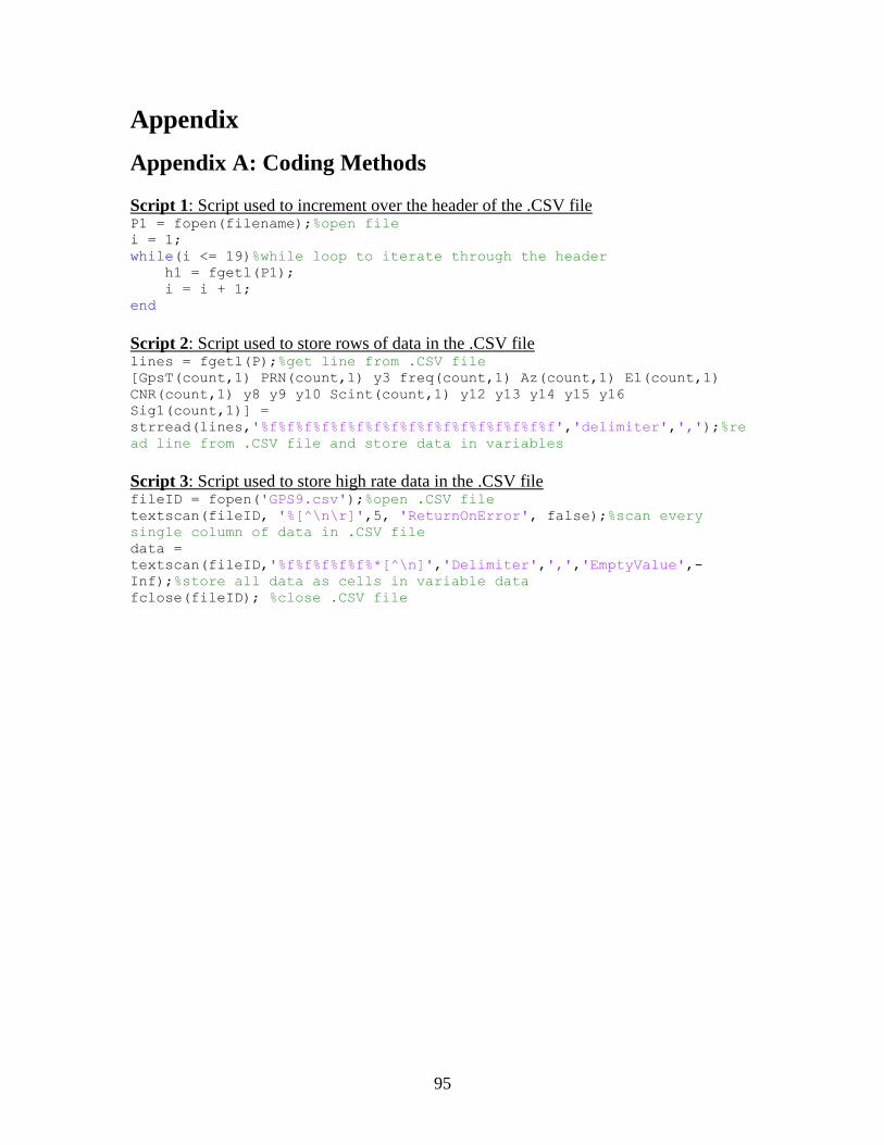
95
Appendix
Appendix A: Coding Methods
Script 1: Script used to increment over the header of the .CSV file P1 = fopen(filename);%open file i = 1; while(i <= 19)%while loop to iterate through the header h1 = fgetl(P1); i = i + 1; end
Script 2: Script used to store rows of data in the .CSV file lines = fgetl(P);%get line from .CSV file [GpsT(count,1) PRN(count,1) y3 freq(count,1) Az(count,1) El(count,1)
CNR(count,1) y8 y9 y10 Scint(count,1) y12 y13 y14 y15 y16
Sig1(count,1)] =
strread(lines,'%f%f%f%f%f%f%f%f%f%f%f%f%f%f%f%f%f','delimiter',',');%re
ad line from .CSV file and store data in variables
Script 3: Script used to store high rate data in the .CSV file fileID = fopen('GPS9.csv');%open .CSV file textscan(fileID, '%[^\n\r]',5, 'ReturnOnError', false);%scan every
single column of data in .CSV file data =
textscan(fileID,'%f%f%f%f%f%*[^\n]','Delimiter',',','EmptyValue',-
Inf);%store all data as cells in variable data fclose(fileID); %close .CSV file