multi-class bio-images classification

ModificationstoaMinimizingExpectedRisk-basedMulti-classImageClassificationAlgorithmonValue-of-Information(VoI)

ZhuoLi—— [email protected]

Abstract—— Real-world image classification always meets with the problem that there are so many images that could be easily obtained through different kinds of technologies, while little of them are correctly labeled manually, for a huge amount of human-labeling requires too much work. However, by applying proper active learning algorithms, computers can complete the labeling process with a small number of human-labeled images as start and interactively querying the oracle or human to get the true labels for some informative images useful in the labeling. In my project, I made some modifications to the existing active learning algorithm [1] on VoI (value-of-information) to perform the task of multi-class image classification. Keywords: Machine Learning; Active Learning; Uncertainty Sampling

IntroductiontothealgorithmIused My algorithm is an adaption to the existing active learning algorithm raised by Joshi, Ajay J., Fatih Porikli, and Nikolaos P. [1] whoseQuery Selection Strategy is Minimizing Expected Risk, from which I modified an Uncertainty Sampling algorithm to implement this multi-class bio-images’ classification project. My adapted algorithm cares about the misclassification risk for every image in the active pool (unlabeled pool) in the query selection phase and uses a support vector machine (SVM) as the base learner. Specifically, I randomly choose 300 samples, which is around 1/10 of the number of query limits, as the “seed” for both the active and random learners, and use a batch mode for Query Selection at the size of 50.

Modifications: In this project, I chose to make modifications to the existing algorithm [1] on the framework of VoI which takes care of two things in the query selection strategy, the misclassification risk and the cost of user annotation. I chose only to consider the metric of misclassification risk rather than the cost of user annotation because in this project, the cost is the same for the algorithm to query for any image in the training set, and there only exists the limit for the number of queries, but the cost for every different query. Hence, misclassification risk is the metric for selecting images to query in active learning. The second modification I made is introduced in the first part of “Why this algorithm is suitable” in the format of “Note”.

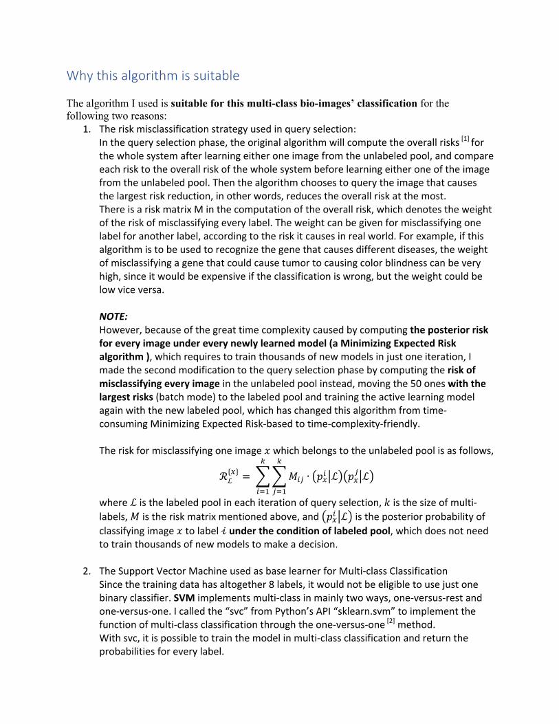
Whythisalgorithmissuitable The algorithm I used is suitable for this multi-class bio-images’ classification for the following two reasons:

1. Theriskmisclassificationstrategyusedinqueryselection:Inthequeryselectionphase,theoriginalalgorithmwillcomputetheoverallrisks[1]forthewholesystemafterlearningeitheroneimagefromtheunlabeledpool,andcompareeachrisktotheoverallriskofthewholesystembeforelearningeitheroneoftheimagefromtheunlabeledpool.Thenthealgorithmchoosestoquerytheimagethatcausesthelargestriskreduction,inotherwords,reducestheoverallriskatthemost.ThereisariskmatrixMinthecomputationoftheoverallrisk,whichdenotestheweightoftheriskofmisclassifyingeverylabel.Theweightcanbegivenformisclassifyingonelabelforanotherlabel,accordingtotheriskitcausesinrealworld.Forexample,ifthisalgorithmistobeusedtorecognizethegenethatcausesdifferentdiseases,theweightofmisclassifyingagenethatcouldcausetumortocausingcolorblindnesscanbeveryhigh,sinceitwouldbeexpensiveiftheclassificationiswrong,buttheweightcouldbelowviceversa.NOTE:However,becauseofthegreattimecomplexitycausedbycomputingtheposteriorriskforeveryimageundereverynewlylearnedmodel(aMinimizingExpectedRiskalgorithm),whichrequirestotrainthousandsofnewmodelsinjustoneiteration,Imadethesecondmodificationtothequeryselectionphasebycomputingtheriskofmisclassifyingeveryimageintheunlabeledpoolinstead,movingthe50oneswiththelargestrisks(batchmode)tothelabeledpoolandtrainingtheactivelearningmodelagainwiththenewlabeledpool,whichhaschangedthisalgorithmfromtime-consumingMinimizingExpectedRisk-basedtotime-complexity-friendly.Theriskformisclassifyingoneimage𝑥whichbelongstotheunlabeledpoolisasfollows,

ℛℒ{%} = 𝑀*+

,

+-.

,

*-.

∙ 𝑝%* ℒ 𝑝%+ ℒ

whereℒisthelabeledpoolineachiterationofqueryselection,𝑘isthesizeofmulti-labels,𝑀istheriskmatrixmentionedabove,and 𝑝%* ℒ istheposteriorprobabilityofclassifyingimage𝑥tolabel𝒾undertheconditionoflabeledpool,whichdoesnotneedtotrainthousandsofnewmodelstomakeadecision.

2. TheSupportVectorMachineusedasbaselearnerforMulti-classClassificationSincethetrainingdatahasaltogether8labels,itwouldnotbeeligibletousejustonebinaryclassifier.SVMimplementsmulti-classinmainlytwoways,one-versus-restandone-versus-one.Icalledthe“svc”fromPython’sAPI“sklearn.svm”toimplementthefunctionofmulti-classclassificationthroughtheone-versus-one[2]method.Withsvc,itispossibletotrainthemodelinmulti-classclassificationandreturntheprobabilitiesforeverylabel.

PerformanceofthisalgorithmBesides the test error as a function of the amount of labeled data declared by the requirements, I used another metric, success rate, to evaluate the performance of the active learner against a random learner, which is actually a projection of test error, documenting the success rate of a model predicting the test set, but more explicitly depicts the successful rates of predictions. Two kinds of images will be provided here for evaluation. In addition, I ran 10 times for EASY and MODERATE dataset to get the average success rate and test error for evaluation, to avoid the randomness of the “seed set” so as to make a more comprehensive evaluation.(Seed set is picked randomly from all training data before the active learning process begins) Note that there is a parameter C in the figures, which is the penalty parameter for SVM and will be explained later in the Findings part. EASYDATASET:

Figure1:One-timeTestErrorsandSuccessRate

versusAmountofLabeledPoints

forEASYdataset

Figure2:AverageTestErrorsandSuccessRate


forEASYdataset

MODERATEDATASET:



forMODERATEdataset

Figure4:AverageTestErrorsandSuccessRate


forEASYdataset

DIFFICULTDATASET:



forDIFFICULTdataset

Findings&ExplanationsofFigures ForParameterCI set C as 1.0 for the EASY and DIFFICULT dataset and 0.9 for the MODERATE dataset, reasons are as follows: C is the penalty parameter for the base learner SVM controlling the influence of the misclassification on the objective function, [3] in other words, parameter C determines the model’s “faith” to training data, that is to say, if C is too large, SVM will “trust” the training data too much, which might cause overfitting. On the contrary, if C is too small, SVM will not “trust” the training data that much, which might cause underfitting. How to choose a better C matters. In SVM, C is default as 1.0, which is a trade-off between bias and variance. For the low-noise EASY and DIFFICULT dataset, I choose C as default, which is 1.0. As for the MODERATE set, since there is some noise in the training data, of which I’ve got to minimize the influence, I choose parameter C as 0.9, which will make the model not “trust” the training data that much so as to avoid overfitting. Four graphs of “success rate” with different Cs are provided in Fig.6 below, from which we can see the difference of the prediction accuracy between active learner and random learner, accounting for the suitability of choosing C as 0.9, rather than other values, for MODERATE set.

Figure6:AverageTestErrorsforMODERATEdataset

withdifferentCs

ForEasyDataset For the EASY dataset, we can observe that the active learner outperforms the random learner, both in the prediction accuracy and the speed to reach its best performance. The active learner has around 77 errors out of 1000 predictions, while the random learner has around 92 errors out of 1000. These are all the final performances of both learners because from Fig.2, the average performance of 10 times of running, we can see the lines for two learners tend to be smooth in the end. From the average performance, we could see that in the beginning, the active learner might perform a little weaker than the random learner, which is because the active learner chooses the most informative images to query, in other words, the ones that are most risky and most likely to be around the boundaries, and the random learner randomly picks images to query, which could temporarily cause the active learner to underperform. However, with the amount of labeled points increasing, we could see crystal clear that the active learner outperforms the random one.

What’s more, the success rate of active learner reaches its peak at 92.4% way before when random learner reaches its peak at 91.1%, which shows that the learning speed of the active learner is faster than the random one. ForModerateDatasetFor the MODERATE dataset, I set penalty parameter C as 0.9 to avoid the influences of noise. We can observe in Fig.4 that the active learner outperforms the random learner, both in the prediction accuracy and the learning speed. The active learner has around 150 errors out of 1000 predictions, while the random learner has around 166 errors out of 1000. From the average performance, we could see that in the beginning, the active learner might perform a little weaker than the random learner, as in the EASY set. However, we could see that overall, the active learner outperforms the random one. The performance in MODERATE set is not as good as in EASY set is because there exists a certain amount of noise in the training set for MODERATE set. In addition, the success rate of the active learner reaches its peak at 85%, and the random learner reaches its peak accuracy is 83.6%. The closer the two learners reach their peaks, the smoother the line of the active learner, which shows that the learning speed of the active learner is faster than the random one. ForDifficultDatasetFor the DIFFICULT dataset, I did feature selection to both before and in each iteration of the active learning. A Tree-based Feature Selection method from Python’s API “sklearn.feature_selection” [4] is applied for feature selection here, and each feature selection is done before training the active learner and random learner to exclude the negative influences of unrelated features. From Fig.7 below, we can see related features in the training data for DIFFUCLT set is around from 23 to 26, which means nearly half the features are unrelated, which are successfully excluded by the process of my feature selection processes.

Figure7:Numbersofselectedfeatures

fortheactiveandrandomlearnersattheend

In addition, by Fig.5, we can see that the active learner has around 130 errors out of 1000 predictions, while the random learner has around 153 errors out of 1000, and nearly in the whole time, the active learner outperforms the random learner with its peak accuracy at 87%, while the random learner’s peak accuracy is 84.7%.

References 1. Joshi, Ajay J., Fatih Porikli, and Nikolaos P. Papanikolopoulos. "Scalable active learning for multiclass image classification." IEEE transactions on pattern analysis and machine intelligence 34.11 (2012): 2259-2273. 2. http://scikit-learn.org/stable/modules/generated/sklearn.svm.SVC.html#sklearn-svm-svc 3. http://stats.stackexchange.com/questions/31066/what-is-the-influence-of-c-in-svms-with-linear-kernel 4. http://scikit-learn.org/stable/modules/feature_selection.html

multi-class bio-images classification

Documents