msc.nastran 2007 implicit nonlinear (sol 600) user's guide
DESCRIPTION
MSC.Nastran Implicit Nonlinear (SOL 600) is an application module in the MSC.Nastran system that pairs the full features of MSC.Nastran with the MSC.Marc solver to analyze a wide variety of structural problems subjected to geometric and material nonlinearities, and contact. An extensive finite element library for building your simulation model, and a set of solution procedures for the nonlinear analysis, which can handle very large matrix equations, are available in MSC.Nastran Implicit Nonlinear(SOL 600).TRANSCRIPT

MSC Nastran 2007 r1
Implicit Nonlinear (SOL 600)User’s Guide

Worldwide Webwww.mscsoftware.com
Disclaimer
This documentation, as well as the software described in it, is furnished under license and may be used only inaccordance with the terms of such license.
MSC.Software Corporation reserves the right to make changes in specifications and other information contained inthis document without prior notice.
The concepts, methods, and examples presented in this text are for illustrative and educational purposes only, and arenot intended to be exhaustive or to apply to any particular engineering problem or design. MSC.Software Corporationassumes no liability or responsibility to any person or company for direct or indirect damages resulting from the useof any information contained herein.
User Documentation: Copyright 2007 MSC.Software Corporation. Printed in U.S.A. All Rights Reserved.
This notice shall be marked on any reproduction of this documentation, in whole or in part. Any reproduction ordistribution of this document, in whole or in part, without the prior written consent of MSC.Software Corporation isprohibited.
The software described herein may contain certain third-party software that is protected by copyright and licensedfrom MSC.Software suppliers.
MSC, MD, Dytran, MSC Fatigue, Marc, MD Patran, MSC Patran Analysis Manager, MSC Patran Laminate Modeler,MSC Patran Materials, MSC Patran Thermal, and PATRAN are trademarks or registered trademarks of MSC.SoftwareCorporation in the United States and/or other countries.
NASTRAN is a registered trademark of NASA. PAM-CRASH is a trademark or registered trademark of ESI Group.SAMCEF is a trademark or registered trademark of Samtech SA. LS-DYNA is a trademark or registered trademark ofLivermore Software Technology Corporation. ANSYS is a registered trademark of SAS IP, Inc., a wholly ownedsubsidiary of ANSYS Inc. ABAQUS is a registered trademark of ABAQUS Inc. ACIS is a registered trademark ofSpatial Technology, Inc. CATIA is a registered trademark of Dassault Systemes, SA. EUCLID is a registered trademarkof Matra Datavision Corporation. FLEXlm is a registered trademark of GLOBEtrotter Software, Inc. HPGL is atrademark of Hewlett Packard. PostScript is a registered trademark of Adobe Systems, Inc. PTC, CADDS andPro/ENGINEER are trademarks or registered trademarks of Parametric Technology Corporation or its subsidiaries inthe United States and/or other countries.Unigraphics, Parasolid and I-DEAS are registered trademarks of ElectronicData Systems Corporation or its subsidiaries in the United States and/or other countries. All other brand names,product names or trademarks belong to their respective owners.
NA*2007R1*Z*INON*Z*DC-USR
CorporateMSC.Software Corporation2 MacArthur PlaceSanta Ana, CA 92707 USATelephone: (800) 345-2078Fax: (714) 784-4056
EuropeMSC.Software GmbHAm Moosfeld 1381829 Munich, GermanyTelephone: (49) (89) 43 19 87 0Fax: (49) (89) 43 61 71 6
Asia PacificMSC.Software Japan Ltd.Shinjuku First West 8F23-7 Nishi Shinjuku1-Chome, Shinjyku-Ku, Tokyo160-0023, JapanTelephone: (81) (03) 6911 1200Fax: (81) (03) 6911 1201

C o n t e n t sMSC Nastran Implicit Nonlinear (SOL 600) User’s Guide
1 Introduction
MSC.Software Products 2
MSC Nastran Implicit Nonlinear (SOL 600) 3Defining the Model 3Nonlinear Analysis 4Results 5
Feature List 7
How SOL 600 Solves Nonlinear Problems 10
This User’s Guide 12Other MSC.Nastran Documentation for SOL 600 12MSC.Marc Documentation 12Patran Documentation 13
2 MSC.Nastran Bulk Data File and Results Files
The MSC.Nastran Bulk Data File 16Input Conventions 17Defaults 18Section Descriptions 18Example 20Running Existing Nonlinear Models 21SOL 600 Executive Control Statement: 21Restart from SOL 600 into SOL 103 or into Another Linear Solution Sequence
26Generating and Editing the Bulk Data File in MSC.Patran 27
Output Requests 28Deformations 28
Results Files 38Files Generated During the Analysis 38Analysis Results Files 38Postprocessing with MSC.Patran 39

MSC Nastran Implicit Nonlinear (SOL 600) User’s Guideiv
Grid Point Force Balance and Element Strain Energy in Nonlinear StaticAnalysis 40
3 Solution Methods and Strategies in Nonlinear Analysis
Introduction 46
Linear Static Analysis Procedure 47
Differences Between Linear and Nonlinear Analysis 48
Applying Constraints 50Single Degrees of Freedom 50Multiple Degrees of Freedom 51
Adding Nonlinear Effects 55Sources of Nonlinearity 55Subcases, Load Increments, and Iterations 56Nonlinear Equation Solution 57SOL 600 Analysis Procedure 59
Numerical Methods in Solving Equations 60Direct Methods 60Iterative Methods 61Preconditioners 61Storage Methods 62Nonsymmetric Systems 63Specifying the Solution Procedure 63Other Factors Affecting Performance 63
Iteration Methods 66Full Newton-Raphson Algorithm 66Modified Newton-Raphson Algorithm 67Strain Correction Method 68The Secant Method 69Specifying the Iteration Method 70
Load Increment Size 71Fixed Load Incrementation 71Adaptive Load (AUTO) Incrementation 71Specifying the Load Incrementation Method 80
Convergence Controls 81Specifying Convergence Criteria 83
Singularity Ratio 84

vCONTENTS
Guidelines for Analysis Methods 86Analysis Methods 86General Tips 86Choosing a Solution Method 86Time Steps or Load Increments 87Nonlinear Dynamics 88Efficiency 88
4 Nonlinearity and Analysis Types
Linear and Nonlinear Analysis 92Linear Analysis 92Nonlinear Analysis 92
Nonlinear Effects and Formulations 93Geometric Nonlinearities 96Material Nonlinearities 106Nonlinear Boundary Conditions 115
Overview of Analysis Types 116
Static Analysis 118Post-Buckling 119Creep, Viscoplastic, and Viscoelastic Behavior 119
Body Approach 120
Buckling Analysis 121Eigenvalue Buckling Prediction 121Bifurcation Approach 122Eigenvalue Extraction Methods 123
Normal Modes 124Eigenvalue Analysis 126Free Vibration Analysis 129Support of Complex Eigenvalue Analysis 130
Transient Dynamic Analysis 132Direct Transient Response 132Technical Background 134Time Step Definition 138Initial Conditions 138Damping 139
Creep 140

MSC Nastran Implicit Nonlinear (SOL 600) User’s Guidevi
5 Analysis Techniques
Domain Decomposition 144Specifying Domain Decomposition 144Single Input File Parallel Processing for SOL 600 146DDM Results in MSC.Patran 146DDM Configuration 147
RESTARTS 148Specifying Restarts and Parameters 148
Inertia Relief with Auto-Support 149Review 149General Formulation 150SUPPORT6 Entry 151
Superelements and Modal Neutral Files 154
BRKSQL 155
User Subroutine Support 159
6 Modeling
Coordinate Systems 162Nodal Coordinate Systems 162Element Coordinate Systems 162
Nodes 164
Elements 165
Modeling in MSC.Patran 166Creating Geometry in MSC.Patran 166Creating Finite Element Meshes in MSC.Patran 168
7 Setting Up, Monitoring, and Debugging the Analysis
Solution Type 172Specifying the Solution Type 172SOL 600 Executive Control Statement 172Defining the Solution Type in MSC.Patran 175
Analysis Procedures 176Analysis Types 176Specifying the Analysis Type for a Subcase 177

viiCONTENTS
Translation Parameters 179Specifying the Translation Parameters 179
Solution Parameters 182Specifying Solution Parameters 182
Subcases 185Specifying Subcases 185
Subcase Parameters 188Specifying Static Subcase Parameters 188Specifying Normal Modes Subcase Parameters 190Specifying Buckling Subcase Parameters 192Specifying Transient Dynamic Subcase Parameters 193Specifying Creep Subcase Parameters 195Specifying Body Approach Subcase Parameters 197
Execution Procedure for MSC.Nastran Implicit Nonlinear from theCommand Line 199
Using MSC.Patran to Execute MSC.Nastran 200How to Tell When the Analysis is Done 200How to Tell if the Analysis Ran Successfully 201
Monitoring the Analysis 202Editing a MSC.Nastran Input File 203
Debugging the Analysis 204Resolving Convergence Problems 204Standard Exit Messages 210Using MSC.Patran to Debug an Analysis 213
8 Output from the Analysis
Overview 216Input 216.OP2 Data 216Results Translation 217
Output Requests 218Specifying Output Requests 218
SOL 600 Results Quantities 226Using MSC.Patran to Postprocess Results Quantities 229
MSC.Nastran Results Quantities 231

MSC Nastran Implicit Nonlinear (SOL 600) User’s Guideviii
Using MSC.Patran to Postprocess MSC.Nastran Results Quantities 231
9 Assigned Conditions
Constraints 236Boundary Conditions 236Multi-Point Constraints 236Support Conditions 247
Loads and Boundary Conditions 248Using MSC.Patran to Apply Loads and Boundary Conditions 250Displacement LBCs 253Force LBCs 254Pressure LBCs 255Temperature LBCs 257Inertial Loads LBCs 259Velocity LBCs 260Acceleration LBCs 261Distributed Load LBCs 261Total Load LBCs 263Contact LBCs 264
Initial Conditions 265Initial Displacement LBCs 265Initial Velocity LBCs 265
10 Materials
Overview 268Constitutive Models 269MSC.Nastran Implicit Nonlinear Material Entries 270
Linear Elastic 272Isotropic Materials 273Orthotropic Materials 274Anisotropic Materials 276
Nonlinear Elastic 278Hypoelastic - Isotropic 278Hyperelastic - Isotropic 278Viscoelastic 305Narayanaswamy Model 315
Inelastic 317

ixCONTENTS
Yield Conditions 318Work Hardening Rules 323Flow Rules 327Rate Dependent Yield 330Experimental Stress-Strain Curves 332Temperature-Dependent Behavior 341Temperature-Dependent Stress Strain Curves 342Specifying Elastoplastic Material Entries 344
Failure and Damage Models 349Isotropic/Orthotropic/Anisotropic Failure Models 349Damage Models 358
Creep 365Oak Ridge National Laboratory Laws 368Viscoplasticity (Explicit Formulation) 369Creep (Implicit Formulation) 369Specifying Creep Material Entries 370
Composite 372Specifying Composite Material Entries 373
Gasket 374Specifying Gasket Material Entries 378
Material Damping 380Specifying Material Damping Entries 381
Experimental Data Fitting 382
11 Element Library
Overview 402Element Types 402
Element Selection 404Element Interpolation 404Element Integration 404Incompressible Elements 405Overriding MSC.Nastran Element Selections 405
Global Element Controls 406Assumed Strain 406Constant Dilatation 406Setting Global Element Parameters in MSC.Patran 406

MSC Nastran Implicit Nonlinear (SOL 600) User’s Guidex
Mass Elements, Springs, Dampers, and Bush Elements 407MSC.Patran FE Application Input Data 407
Gap Elements 409MSC.Patran FE Application Input Data 409
Line Elements 410MSC.Patran FE Application Input Data 410
Membranes, Panels, and Shells 411MSC.Patran FE Application Input Data 412
Solid Elements 413Axisymmetric Elements 414Plane Strain Elements 4143-D Solid Elements 416
Beam/Bar and Shell Offsets 417
12 Contact
Overview 420
Contact Methodology 421Contact Bodies 421Numerical Procedures 430Implementation of Constraints 434Separation 436Higher Order Elements 4373-D Beam and Shell Contact 437Friction Modeling 438
Defining Contact Bodies 447Deformable and Rigid Surfaces 447Motion of Surfaces 447Cautions 448Control Variables and Option Flags 448Time Step Control 449Dynamic Contact - Impact 449Two-dimensional Rigid Surfaces 449Specifying Contact Body Entries 462
Selecting and Controlling Contact Behavior 467Contact Parameters 467Contact Table 471Movement of Contact Bodies 475

xiCONTENTS
Initial Conditions 476
Simulating Thermal Contact 477Input 477
References 480
13 SOL 600 Example Problems
Engine Gasket Under Bolt Preload 482Problem Statement 482Model Description 483Solving the Problem 485Inspecting the Results 489
Elastic-Plastic Collapse of a Cylindrical Pipe under External Rigid BodyLoading 491
Problem Statement 491Model Description 492Solving the Problem 494Inspecting the Results 497
Rubber Door Seal - Performance Door Closing 500Problem Statement 500Model Description 500Solving the Problem 501Inspecting the Results 504
Brake Forming 505Problem Statement 505Model Description 505Solving the Problem 506Inspecting the Results 509
Panel Buckling 510Problem Statement 510Model Description 510Solving the Problem 512Inspecting the Results 514
Index 515

MSC Nastran Implicit Nonlinear (SOL 600) User’s Guidexii

Technical Resources MD Nastran Quick Reference Guide
Technical Resources
List of Nastran Books xx
Technical Support xxi
Internet Resources xxiii

MD Nastran Quick Reference GuideList of Nastran Books
xx
List of Nastran BooksBelow is a list of some of the Nastran documents. You may order any of these documents from theMSC.Software BooksMart site at http://store.mscsoftware.com.
Installation and Release Guides
Installation and Operations Guide
Release Guide
Reference Books
Quick Reference Guide
DMAP Programmer’s Guide
Reference Manual
User’s Guides
Getting Started
Linear Static Analysis
Basic Dynamic Analysis
Advanced Dynamic Analysis
Design Sensitivity and Optimization
Thermal Analysis
Numerical Methods
MD User’s Guide
Implicit Nonlinear (SOL 600)
Explicit Nonlinear (SOL 700)
Aeroelastic Analysis
Superelement
User Modifiable
Toolkit

xxiTechnical ResourcesTechnical Support
Technical SupportFor help with installing or using an MSC.Software product, contact your local technical support services.Our technical support provides the following services:
• Resolution of installation problems
• Advice on specific analysis capabilities
• Advice on modeling techniques
• Resolution of specific analysis problems (e.g., fatal messages)
• Verification of code error.
If you have concerns about an analysis, we suggest that you contact us at an early stage.
You can reach technical support services on the web, by telephone, or e-mail:
Web Go to the MSC.Software website at www.mscsoftware.com, and click onSupport. Here, you can find a wide variety of support resources includingapplication examples, technical application notes, available training courses, anddocumentation updates at the MSC.Software Training, Technical Support, andDocumentation web page.
Phone and Fax United StatesTelephone: (800) 732-7284Fax: (714)
Frimley, CamberleySurrey, United KingdomPhone: (44) (1276) 60 19 00Fax: (44) (1276) 69 11 11
Munich, GermanyPhone: (49) (89) 43 19 87 0Fax: (49) (89) 43 61 71 6
Tokyo, JapanPhone: (81) (3) 3505 02 66Fax: (81) (3) 3505 09 14
Rome, ItalyPhone: (390) (6) 5 91 64 50Fax: (390) (6) 5 91 25 05
Paris, FrancePhone: (33) (1) 69 36 69 36Fax: (33) (1) 69 36 45 17
Moscow, RussiaPhone: (7) (095) 236 6177Fax: (7) (095) 236 9762
Gouda, The Netherlands:Phone: (31) (18) 2543700Fax: (31) (18) 2543707
Madrid, SpainPhone: (34) (91) 5560919Fax: (34) (91) 5567280

MD Nastran Quick Reference GuideTechnical Support
xxii
E-mail Send a detailed description of the problem to the email address below thatcorresponds to the product you are using. You should receive an acknowledgementthat your message was received, followed by an email from one of our TechnicalSupport Engineers.
MD Patran Support
MD Nastran Support
Dytran Support
MSC Fatigue Support
Marc Support
MSC Institute Course Information

xxiiiTechnical ResourcesInternet Resources
Internet Resources
MSC.Softwarewww.mscsoftware.com)
MSC.Software corporate site with information on the latest events, products and services for theCAD/CAE/CAM marketplace.
TrainingThe MSC Institute of Technology is the world's largest global supplier of CAD/CAM/CAE/PDMtraining products and services for the product design, analysis and manufacturing market. We offer over100 courses through a global network of education centers. The Institute is uniquely positioned tooptimize your investment in design and simulation software tools.
Our industry experienced expert staff is available to customize our course offerings to meet your uniquetraining requirements. For the most effective training, The Institute also offers many of our courses atour customer's facilities.
The MSC Institute of Technology is located at:
2 MacArthur PlaceSanta Ana, CA 92707Phone: (800) 732-7211Fax: (714) 784-4028
The Institute maintains state-of-the-art classroom facilities and individual computer graphics laboratoriesat training centers throughout the world. All of our courses emphasize hands-on computer laboratorywork to facility skills development.
We specialize in customized training based on our evaluation of your design and simulation processes,which yields courses that are geared to your business.
In addition to traditional instructor-led classes, we also offer video and DVD courses, interactivemultimedia training, web-based training, and a specialized instructor's program.
Course Information and Registration
For detailed course descriptions, schedule information, and registration call the Training Specialist at(800) 732-7211 or visit www.mscsoftware.com.

MD Nastran Quick Reference GuideInternet Resources
xxiv

MSC.Nastran 2005 r3 Implicit Nonlinear (SOL 600) User’s Guide
Ch. 1: Introduction
1 Introduction
MSC.Software Products 2
MSC Nastran Implicit Nonlinear (SOL 600) 3
Feature List 7
How SOL 600 Solves Nonlinear Problems 10
This User’s Guide 12

MSC.Nastran 2007 r1 Implicit Nonlinear (SOL 600) User’s Guide2
MSC.Software ProductsMSC.Software Corporation provides an extensive array of software products that make it possible tosimulate almost any engineered component with any level of detail you require. MSC is recognized as aleader in finite element analysis software with a product list that includes MSC.Nastran, MSC.Patran,MSC.Marc, MSC.Dytran and many others. Each of these codes within themselves are powerful general-purpose analysis codes that can be used to solve structural, heat transfer, and coupled thermal-structuralfinite element problems. When paired together and supplemented with special purpose applicationmodules and interfaces these software products can be tailor made to suit specific industries andengineering problems unique to those industries.

3CHAPTER 1Introduction
MSC Nastran Implicit Nonlinear (SOL 600)MSC.Nastran Implicit Nonlinear (SOL 600) is an application module in the MSC.Nastran system thatpairs the full features of MSC.Nastran with the MSC.Marc solver to analyze a wide variety of structuralproblems subjected to geometric and material nonlinearities, and contact. An extensive finite elementlibrary for building your simulation model, and a set of solution procedures for the nonlinear analysis,which can handle very large matrix equations, are available in MSC.Nastran Implicit Nonlinear(SOL 600).
The MSC.Nastran Implicit Nonlinear product is rapidly evolving. This document is based upon the2005 r3 release and should be used with this or subsequent versions.
Defining the ModelA finite element model consists of a geometric description, which is given by the elements and theirnodes and a set of properties associated with the elements, describing their attributes. These propertiesinclude material definitions, cross-section definitions in the case of structural elements like beams andshells, and other parameters for contact bodies, springs, dashpots, etc. There may also be constraints thatmust be included in the model - RBE elements, or “multi-point constraints'' or “equations'' (linear ornonlinear equations involving several of the fundamental solution variables in the model), or simple“boundary conditions'' that are to be imposed throughout the analysis. Nonzero initial conditions, suchas initial temperatures, displacements, velocities, and even initial stresses and/or plastic strains may alsobe specified.
The model is described and communicated to MSC.Nastran in the form of a text file, called aMSC.Nastran Input file. You can generate this file using any text editor, but it must adhere toMSC.Nastran conventions for the ordering and format of the model information.
Using MSC.Patran with SOL 600
The amount of information that needs to be conveyed in the MSC.Nastran Input file is extensive for evena modest size model. The amount of information and the complexity of most models makes it virtuallyimpossible to generate the MSC.Nastran Input file with a text editor alone. Typically you benefit fromusing a preprocessor such as, MSC.Patran. MSC.Patran is another MSC Software simulation code thatprovides a graphical user interface and an extensive line of model building tools that you can use toconstruct and view your model, and generate a MSC.Nastran Input file.
If you are using MSC.Patran as a preprocessor, you are required to specify an analysis code. SelectingMSC.Nastran Implicit Nonlinear (SOL 600) as the analysis code under the Analysis Preference menu,customizes MSC.Patran in five main areas:
• Material Library
• Element Library
• Loads and Boundary Conditions
• MPCs
• Analysis forms

MSC.Nastran 2007 r1 Implicit Nonlinear (SOL 600) User’s Guide4
The analysis preference also specifies that the model information be output in the MSC.Nastran InputFile format.
Throughout this Users Guide, actual examples are described in the context of using MSC.Patran. ActualMSC.Patran forms and instructions are provided.
Nonlinear AnalysisLinear analysis assumes a linear relationship between the load applied to a structure and the response ofthe structure. The stiffness of a structure in a linear analysis does not change depending on its previousstate. Linear static problems are solved in one step, by a single decomposition of the stiffness matrix. Anumber of important assumptions and limitations are inherent in linear static analysis. Materials behavioris such that the stress is directly proportional to strain (linear) and to loads that do not take the materialbeyond its permanent yield point (the material remains elastic). Linear analysis is restricted to smalldisplacements, otherwise the stiffness of the structures changes and must be accounted for byregenerating the stiffness matrix. Lastly, loads are assumed to be applied slowly as to keep the structurein equilibrium.
It becomes necessary to consider nonlinear effects in structures when modeling materials with nonlinearbehavior and where large deformations (rotations and/or strains) occur. In addition, contact problemsexhibit nonlinear effects due to changes in boundary conditions.
In a nonlinear problem the stiffness of the structure depends on the displacement and the response is nolonger a linear function of the load applied. As the structure displaces due to loading, the stiffnesschanges, and as the stiffness changes the structure’s response changes. As a result, nonlinear problemsrequire incremental solution schemes that divide the problem up into steps calculating the displacement,then updating the stiffness. Each step uses the results from the previous step as a starting point. As a resultthe stiffness matrix must be generated and decomposed many times during the analysis adding time andcosts to the analysis.
Nonlinear problems present many challenges. A nonlinear problem does not always have a uniquesolution. Sometimes a nonlinear problem does not have any solution, although the problem can seem tobe defined correctly.
Nonlinear analysis requires choosing a solution strategy which includes dividing the loading into logicalsteps, controlling the numerical processing, and planning for the possibility of changing the solutionstrategy during the analysis using restarts. Which solution method to use depends on the structure itself,the nature of the loading, and the anticipated nonlinear behavior. In some cases, one method can beadvantageous over another; in other cases, the converse might be true.
If a solution is obtainable, there is also the issue of efficiency. Each solution procedure, has pros and consin terms of matrix operations and storage requirements. In addition, a very important variable regardingoverall efficiency is the size of the problem. The time required to assemble a stiffness matrix, as well asthe time required to recover stresses after a solution, vary roughly linearly with the number of degrees offreedom of the problem. On the other hand, when using a direct solver the time required to go throughthe solver varies roughly quadratically with the bandwidth, as well as linearly with the number of degreesof freedom.

5CHAPTER 1Introduction
Applications for Nonlinear Analysis
Early development of nonlinear finite element technology was mostly influenced by the nuclear andaerospace industries. In the nuclear industry, nonlinearities are mainly due to high-temperature behaviorof materials. Nonlinearities in the aerospace industry are mainly geometric in nature and range fromsimple linear buckling to complicated post-bifurcation behavior. Nonlinear finite element techniqueshave become popular in metal forming manufacturing processes, fluid-solid interaction, and fluid flow.In recent years, the areas of biomechanics and electromagnetics have seen an increasing use of finiteelements.
ResultsLike the enormous amount of data needed to define the simulation model to an analysis code, there is alarge volume of data returned from the simulation analysis. And just as it is virtually impossible toconstruct a model with a text editor alone, it is equally as difficult to read and interpret the results byhand. Using a postprocessor with a graphical user interface such as MSC.Patran is highly recommended.
Postprocessing Features of MSC.Patran
The MSC.Patran Results application gives you control of powerful graphical capabilities to displayresults quantities in a variety of ways:
• Deformed structural plots
• Color banded fringe plots
• Marker plots (vectors, tensors)
• Freebody diagrams
• Graph (XY) plots
• Animations of most of these plot types.
The Results application treats all results quantities in a very flexible and general manner. In addition, formaximum flexibility results can be:
• Sorted
• Reported
• Filtered
• Derived
• Deleted
All of these features help give meaningful insight into results interpretation of engineering problems thatwould otherwise be difficult at best.

MSC.Nastran 2007 r1 Implicit Nonlinear (SOL 600) User’s Guide6
The Results application is object oriented, providing postprocessing plots which are created, displayed,and manipulated to obtain rapid insight into the nature of results data. The imaging is intended to providegraphics performance sufficient for real time manipulation. Performance will vary depending onhardware, but consistency of functionality is maintained as much as possible across all supported displaydevices.
Capabilities for interactive results postprocessing also exist. Advanced visualization capabilities allowcreation of many plot types which can be saved, simultaneously plotted, and interactively manipulatedwith results quantities reported at the click of the mouse button to better understand mechanical behavior.Once defined, the visualization plots remain in the database for immediate access and provide the meansfor results manipulation and review in a consistent and easy to use manner.

7CHAPTER 1Introduction
Feature ListThe complete features of MSC.Nastran Implicit Nonlinear (SOL 600) are presented in the following list.
1. MSC.Nastran Implicit Nonlinear (SOL 600) solves linear and nonlinear (material, contact and/orgeometric) static, modal (vibration), buckling, and transient dynamic structural finite elementproblems.
2. Eigenvalue solutions are available in MSC.Nastran Implicit Nonlinear (SOL 600) for solvinglinear or nonlinear modal and buckling analyses using either Lanczos or Inverse Power Sweepmethods of iteration. Through the use of parameters you can control the convergence of theeigenvalues, and the modes to retain.
3. MSC.Nastran Implicit Nonlinear (SOL 600) has a variety of solution procedures and bandwidthoptimizers.
4. MSC.Nastran Implicit Nonlinear (SOL 600) supports the following elements/bodies:
• 3 and 6 noded triangular shell/membrane/plane stress/(generalized) plain strain/axisymmetricelements
• 4 and 8 noded quadrilateral shell/membrane/plane stress/(generalized) plainstrain/axisymmetric elements
• 4 and 10 noded solid tetrahedral elements
• 6 and 15 noded solid wedge elements
• 8 and 20 noded solid hexahedral elements
• 2 and 3 noded beam element
• 2 and 3 noded bar element
• 2 and 3 noded axisymmetric shell element
• 2 noded gap element
• 1 and 2 noded spring elements
• 1 and 2 noded damper elements
• Rigid and deformable contact bodies
• Point Mass element
RBE elements and multi-point constraint equations are supported in MSC.Nastran ImplicitNonlinear (SOL 600) to tie specific nodes or degrees-of-freedom to each other. Special MPCentities are supported, (e.g. rigid links) which can be used to tie two nodes together or equate themotion of two DOFs.

MSC.Nastran 2007 r1 Implicit Nonlinear (SOL 600) User’s Guide8
5. MSC.Nastran Implicit Nonlinear (SOL 600) supports the following loads and boundaryconditions:
• Constrained nodal displacements (zero displacements at specifieddegrees-of-freedom).Enforced nodal displacements (non-zero displacements at specifieddegrees-of-freedom in the nodal coordinate system).
• Forces applied to nodes in the nodal coordinate system.
• Pressures applied to element edges or faces, including strain-rate controlled application forsuper-plastic forming simulations.
• Temperature applied to nodes. Temperature can be applied as a load in a structural analysis.The reference temperature is user definable.
• Inertial body forces, acceleration and velocity can be applied in the global coordinate system.
• Contact between two bodies can be defined by selecting the contacting bodies and definingthe contact interaction properties.
6. MSC.Nastran Implicit Nonlinear (SOL 600) supports isotropic, orthotropic and anisotropicmaterial properties. Temperature dependent isotropic and orthotropic material properties can bedefined for elastic, elastic-plastic, hyper-elastic, visco-elastic, and creep constitutive models.Nonlinear elastic-plastic materials can be defined by specifying piecewise linear stress-straincurves, which may be temperature dependent.
7. Physical properties can be associated with MSC.Nastran Implicit Nonlinear (SOL 600) elementssuch as the cross-sectional properties of the beam element, the area of the beam and rod elements,the thickness of shell, plane stress, and membrane elements, spring parameters, masses, gapelement parameters, the alternate material coordinate frame for solid elements and material IDs.
8. Laminated composite solid and shell elements are supported in MSC.Nastran Implicit Nonlinear(SOL 600) through the PCOMP card of the materials capability. Each layer has its own material,thickness, and orientation and may represent linear or nonlinear material behavior. Failure indexcalculations are also supported. Equivalent material models may be incorporated using PSHELL.
9. Analysis jobs consisting of (possibly) complex loading histories (such as would occur in a multi-step manufacturing process) for MSC.Nastran Implicit Nonlinear (SOL 600) are defined usingsubcases. A single subcase may represent the entire analysis, or may be one step in a multi-stepsimulation. The loads and constraints in each subcase represent the total load at that point in theanalysis, making it easy to determine the state of loading at any point in the analysis. The startingpoint of the current subcase is the ending point of the previous subcase.
10. MSC.Nastran Implicit Nonlinear (SOL 600) jobs are submitted using text-based input decks thatmay be generated manually with a text editor, or by a variety of pre/post processing programs suchas MSC.Patran. The input file is read in and a number of text files, such as the .f06, .log, .f04 filesare generated.
11. Results can be requested in several output formats such as .f06, .t16, .t19, .xdb, .op2, or punchfiles. These files are typically read back into the pre/post processing programs for the purpose ofevaluating the results with plots such as deformed shape plots, contour stress/strain plots, or X-Yhistory plots.

9CHAPTER 1Introduction
12. Nodal displacements, velocities and accelerations, mode shapes, element and nodal stresses,element and nodal strains, element and nodal plastic strains, element and nodal creep strains,nodal reaction forces and contact interface stress/force values, shell element stress resultants,element strain energy, strain energy density, and phase angle values can all be requested as outputand visualized with the aforementioned results visualization tools such as MSC.Patran. Stressfunctions, for example von Mises, beam stresses, strains, and internal forces, can also berequested as output. Composite element results are returned for each layer of the composite.
13. A restart capability is available in MSC.Nastran Implicit Nonlinear (SOL 600). Any analysis canbe saved from any point for a possible restart. A new static load case or a buckling analysis canbe solved by restarting from the original static analysis.

MSC.Nastran 2007 r1 Implicit Nonlinear (SOL 600) User’s Guide10
How SOL 600 Solves Nonlinear ProblemsThe primary steps in running a MSC.Nastran Implicit Nonlinear (SOL 600) analysis are as follows:
1. Read MSC.Nastran Input File in IFP (input file processor) as in other MSC.Nastran solutionsequences.
2. Convert MSC.Nastran input to MSC.Marc input and write out a MSC.Marc input deck(jid.marc.dat in IFP).
3. If there are no input errors, execute MSC.Marc.
4. If you request, do any of the following:
5. Translate MSC.Marc’s t16 file to obtain MSC.Nastran op2 or xdb output (this is done by code inMSC.Nastran that creates output op2 data blocks on a file, which we call the f11 file, thengenerating DMAP on the fly to use inputt2 to placed the f11 datablocks into the MSC.Nastrandatabase, and finally use OUTPUT2 to produce an OP2 file which has the geometry datablocksand the f11 output datablocks all in one file (or similar DMAP to generate an xdb file withgeometry and output datablocks.
6. As in Step 5, DMAP can be extended to produce printed output in the.f06 file or punched outputin the .pch file having the exact formats MSC.Nastran uses for all other solution sequences (thisis done by generating OFP DMAP on the fly).
7. Copy MSC.Marc’s output file (known as the .out file) to the .f06 file with or without changingany text strings. This output will have the MSC.Marc formats, but names such as MSC.Marc canbe changed to any desired user name (for example MSC.Nastran Implicit Nonlinear). It is stronglysuggested that Steps 6 and 7are not both done in the same run, or the f06 file output could becomeconfusing.
8. Retain or delete the MSC.Marc input and output files (which normally consist of jid.marc.dat,jid.marc.out, jid.marc.sts, jid.marc.log, jid.marc.t16 and possibly others which have the namejid.marc.*).
The process of reading input data from a MSC.Nastran Input File, translating the model data to aMSC.Marc input file, running a MSC.Marc solution, and translating back the results files is shown in theflowchart that follows.

11CHAPTER 1Introduction
Figure 1-1 MSC.Nastran Implicit Nonlinear (SOL 600) Solution Process
MSC.Nastran Input Deck
Use std Nast output req -
deck echo and
Write jobname.marc.dat
IFP Processes Input Deck
Stop
SuccessfulTranslation?
Submit MarcAnalysis?
Marc writes.out,.t16,.t19
Is marccpy= 1or 2?
Submit Marc job -see note
Append runtime error
.t16/19 results to Nast db
Nastran.f06,.f04, .log files
error messages
Yes
Yes
Yes
generate std xdb,op2,f06
.sts, etc (these will bedeleted later by Nastranif marccpy = 1 or 3) -.sts
messages to .f06 and .log
and .log may be used byMSC.Patran to monitorthe progress of the jobwhile it is running
Note - every attempt will bemade to have the MSC.Nastran InputFile Processor (IFP) catch allinput format errors. However,this may not be possiblein all cases and sometimes it isnecessary for youto examine the MSC.Marc .dat files
No
No
No
for errors.

MSC.Nastran 2007 r1 Implicit Nonlinear (SOL 600) User’s Guide12
This User’s GuideThis manual provides a complete background to SOL 600 and fully describes using SOL 600 within theMSC.Nastran environment. The theoretical aspects of nonlinear analysis methods, types, and techniquesare included as well as thorough descriptions for nonlinear material models.
Where appropriate, actual MSC.Patran forms and menus are shown so you can easily use SOL 600 fromthe MSC.Patran environment.
Other MSC.Nastran Documentation for SOL 600
MSC.Nastran Reference Manual
The MSC.Nastran Reference Manual provides supporting information that relates to MSC.Nastran inputformats, element libraries, and loads and boundary conditions.
Quick Reference Guide (QRG)
The QRG contains a complete description of all the input entries for MSC.Nastran. Within each section,entries are organized alphabetically so they are easy to find. Each entry provides a description, formats,examples, details on options, and general remarks.
You will find the full descriptions for all SOL 600 input entries in the QRG.
MSC.Marc DocumentationMSC provides extensive documentation covering all aspects of the MSC.Marc code. In particular thefollowing manuals are recommended to use in conjunction with SOL 600:
• MSC.Marc Volume A: Theory and User Information - explains the capabilities of MSC.Marcand gives pertinent background information.
• MSC.Marc Volume C: Program Input - describes the file format of the MSC.Marc input file.\
• MSC.Macr Volume D: User subroutines and special routines - describes format for usersubroutines.

13CHAPTER 1Introduction
Patran DocumentationThree key books from the Patran library may be of assistance in running SOL 600:
• Patran User’s Guide - this introductory guide gives you the essential information you need toimmediately begin using MSC.Patran for SOL 600 projects. Understanding and using theinformation in this guide requires no prior experience with CAE or finite element analysis.
• Patran Reference Manual -a counterpart to the MSC.Nastran Reference Manual, this manualprovides complete descriptions of basic functions in MSC.Patran, geometry modeling, finiteelement modeling, material models, element properties, loads and boundary conditions,analysis, and results.
• MSC Nastran Preference Guide - gives specific information that relates to using MSC.Patranwith MSC.Nastran as the intended analysis code. All application forms and required input aretailored to MSC.Nastran.

MSC.Nastran 2007 r1 Implicit Nonlinear (SOL 600) User’s Guide14

MSC.Nastran 2005 r3 Implicit Nonlinear (SOL 600) User’s Guide
Ch. 2: MSC.Nastran Bulk Data File and Results Files
2 MSC.Nastran Bulk Data File andResults Files
The MSC.Nastran Bulk Data File 16
Output Requests 28
Results Files 38

MSC.Nastran 2007 r1 Implicit Nonlinear (SOL 600) User’s Guide16
The MSC.Nastran Bulk Data FileThe MSC.Nastran Input File, referred to as the Bulk Data File (BDF) is made up of three distinct sections:
1. Executive Control - describes the problem type and size.
2. Case Control - defines the load history.
3. Bulk Data - gives a detailed model description.
Input data is organized in (optional) blocks. Key words identify the data for each optional block. Thisform of input enables you to specify only the data for the optional blocks that you need to define yourproblem. The various blocks of input are “optional” in the sense that many have built-in default valueswhich can be used in the absence of any explicit input from you.
A typical input file setup for the MSC.Nastran program is shown below.
• Executive Control StatementsTerminated by an CEND parameter
• Case Control CommandsTerminated by the BEGIN BULK option
• Bulk Data EntriesModel data starting with the BEGIN BULK option and terminated by the ENDDATA option
IFP (Input File Processing) Checking
Checking of most SOL 600 Bulk Data entries are done during IFP. When one of these entrieshas erroneous data entered it is more likely that IFP will flag the entry and issue a FATALERROR. In most cases, IFP error checking has been enhanced to point to the field andcontinuation line where the erroneous data occurs.
• (Additional History DefinitionOption for the second, third, ..., Increments).

17CHAPTER 2MSC.Nastran Bulk Data File and Results Files
Input ConventionsMSC.Nastran Implicit Nonlinear performs all data conversion internally so that the system does not abortbecause of data errors made by you. The program reads all input data options alphanumerically andconverts them to integer, floating point, or keywords, as necessary. MSC Nastran Implicit Nonlinearissues error messages and displays the illegal option image if it cannot interpret the option data fieldaccording to the specifications given in the manual. When such errors occur, the program attempts toscan the remainder of the data file and ends the run with a FATAL ERROR or SEVERE WARNINGmessage.
Two input format conventions can be used: fixed and free format. You can mix fixed and free formatoptions within a file.
The syntax rules for fixed fields are as follows:
• Give floating point numbers with or without an exponent. If you give an exponent, it must bepreceded by the character E or D and must be right-justified. If data is double precision, a Dmust be used.
Bulk Data
Case Control
Executive Control
Element andMaterialProperties,Fixed Displ,
Load Incrementation,Applied Loads,Applied DisplacementsEtc.
Title, Job Control,Solution Sequence,Etc.
Com
plet
eIn
putD
eck
Con
trol
Info
rmat
ion
Mod
elD
ata
-gr
ids,
elem
ents
,etc
.Etc.

MSC.Nastran 2007 r1 Implicit Nonlinear (SOL 600) User’s Guide18
The syntax rules for free fields are as follows:
• Check that each option contains the same number of data items that it would contain understandard fixed-format control. This syntax rule allows you to mix fixed-field and free-fieldoptions in the data file because the number of options you need to input any data list are the samein both cases.
• Separate data items on a option with a comma. The comma can be surrounded by any number ofblanks. Within the data item itself, no embedded blanks can appear.
• Give floating point numbers with or without an exponent. If you use an exponent, it mustbe preceded by the character E or D and must immediately follow the mantissa (no embeddedblanks).
• Give keywords exactly as they are written in the manual.
• All data can be entered as uppercase or lowercase text.
• Small field format is limited to 8 columns per field. Large field is 16 columns, see the MDNastran Quick Reference Guide for more details.
DefaultsFor most bulk data entries, SOL 600 does not make the distinction between zero and blank. Thus, if azero is entered and the default is some other value, the default will normally be used. If you wish to usezero, enter a small number such as 1.0E-12 instead.
Section Descriptions
Executive Control
This group of entries provides overall job control for the problem and sets up initial switches to controlthe flow of the program through the desired analysis. This set of input must be terminated with an CENDparameter. See Executive Control Statements (Ch. 3) in the for additional descriptions on input formats.
Case Control
This group of options provides the loads and constraints and load incrementation method and controlsthe program after the initial elastic analysis. Case Control options also include blocks which allowchanges in the initial model specifications. Case Control options can also specify print-out andpostprocessing options. Each set of load sets must be begin with a SUBCASE command and beterminated by another SUBCASE or a BEGIN BULK command. If there is only one load case, theSUBCASE entry is not required. The SUBCASE option requests that the program perform anotherincrement or series of increments. See Case Control Command Descriptions (Ch. 4) in the for additionaldescriptions on input formats.

19CHAPTER 2MSC.Nastran Bulk Data File and Results Files
Bulk Data Entries
This set of data options enters the initial loading, geometry, and material data of the model and providesnodal point data, such as boundary conditions. Bulk data options are also used to govern the error controland restart capability.This group of options must be terminated with the ENDDATA option. See BulkData Entries (Ch. 8) in the for additional descriptions on input formats. Multiple BEGIN entries andsuperelements are not allowed in SOL 600.

MSC.Nastran 2007 r1 Implicit Nonlinear (SOL 600) User’s Guide20
ExampleThe following text illustrates a simple example of an MSC.Nastran Implicit Nonlinear input file. Itincludes the required Executive Control, Case Control, and Bulk Data sections that are required for anyMSC.Nastran analysis.
$ NASTRAN input file created by the MSC MSC.Nastran input file$ translator (MSC.Patran 2004) on February 03, 2003 at 15:09:41.$ Direct Text Input for File Management Section$ Advanced Nonlinear AnalysisSOL 600,106 PATH=1 STOP=1CENDSEALL = ALLSUPER = ALLTITLE = MSC.Nastran job created on 03-Feb-03 at 15:04:03$ Direct Text Input for Global Case Control DataSUBCASE 1$ Subcase name : Default
SUBTITLE=DefaultNLPARM = 1SPC = 2LOAD = 2DISPLACEMENT(SORT1,REAL)=ALLSPCFORCES(SORT1,REAL)=ALLSTRESS(SORT1,REAL,VONMISES,BILIN)=ALL
$ Direct Text Input for this SubcaseBEGIN BULKPARAM PRTMAXIM YESNLPARM 1 10 AUTO 1 25 P YES$ Direct Text Input for Bulk Data$ Elements and Element Properties for region : shell_propsPSHELL 1 1 .253 1 1$ Pset: "shell_props" will be imported as: "pshell.1"CQUAD4 1 1 1 2 5 4CQUAD4 2 1 2 3 6 5CQUAD4 3 1 4 5 8 7CQUAD4 4 1 5 6 9 8$ Referenced Material Records$ Material Record : steel$ Description of Material : Date: 03-Feb-03 Time: 15:01:32MAT1 1 3.+7 .3 .0075$ Nodes of the Entire ModelGRID 1 0. 0. 0.GRID 2 5. 0. 0.GRID 3 10. 0. 0.GRID 4 0. 5. 0.GRID 5 5. 5. 0.GRID 6 10. 5. 0.GRID 7 0. 10. 0.GRID 8 5. 10. 0.GRID 9 10. 10. 0.$ Loads for Load Case : DefaultSPCADD 2 1$ Displacement Constraints of Load Set : fix_edgeSPC1 1 123456 1 4 7$ Contact Table for Load Case: Default$ Nodal Forces of Load Set : point_loadFORCE 1 9 0 100. 0. 0. -1.$ Referenced Coordinate FramesENDDATA

21CHAPTER 2MSC.Nastran Bulk Data File and Results Files
Running Existing Nonlinear ModelsSome users may have existing models that have been developed and analyzed using MSC.NastranNonlinear Solution Sequences 106 or 129. These models may be run through MSC.Nastran ImplicitNonlinear (SOL 600) by changing the SOLUTION procedure input to MSC.Nastran Implicit Nonlinear(SOL 600) input.
The following is an example of the change required to run existing models through SOL 600. The firstline shows an existing MSC.Nastran SOL 106 Executive Control Statement and the second shows itsrevision for MSC.Nastran Implicit Nonlinear (SOL 600).
SOL 106SOL 600,106
SOL 600 Executive Control Statement:The new executive control statement is as follows:
SOL 600, ID PATH= COPYR= NOERROR OUTR=op2,xdb,pch,f06,eig,dmap,beam, NOEXIT STOP=CONTINUE= S67OPT=
Some items such as dmap, beam, CONTINUE and S67OPT are explained here. See the MSC.NastranQRG for a complete discussion. An explanation of these items follows:
CONTINUE=
CONTINUE= An option that specifies how MSC.Nastran will continue its analysis after MSC.Marcfinishes. To continue the analysis, do not enter any STOP or OUTR options. It is possible to performmore than one of these operations if necessary.
dmap The user will enter his own DMAP to create whatever type of output that is desired, such asop2, xdb, punch, f06. For all other options, DMAP as needed is generated internally byMSC.Nastran.
beam The beam option must be specified if op2,xdb,pch. or f06 options are specified and beaminternal loads are to be placed in any of these files. The beam and eig options are mutuallyexclusive (you cannot specify both).

MSC.Nastran 2007 r1 Implicit Nonlinear (SOL 600) User’s Guide22
0 MSC.Nastran will continue the current solution sequence as normal. For example, if SOL600,106 is entered, SOL 106 will continue as normal after MSC.Marc finishes. Only 3-Dcontact or materials supported by SOL 106 may be used.
1 MSC.Nastran will continue the current solution sequence as normal. For example if SOL600,106 is entered, SOL 106 will continue as normal after MSC.Marc finishes. Of course, no3-D contact or materials not supported by SOL 106 may be used.
2 MSC.Nastran will switch to SOL 107 to compute complex eigenvalues. MSC.Marc willgenerate DMIG matrices for friction stiffness (and possibly damping) on a file specified bypram,marcfil1,name and time specified by param,marcstif,time. This is accomplished bymaking a complete copy of the original MSC.Nastran input file and spawning off a new jobwith the SOL entry changed and an include entry for the DMIG file.
3 (Option not presently available.) MSC.Nastran will switch to SOL 107 to compute complexeigenvalues. MSC.Marc will generate OUTPUT4 matrices for friction stiffness (and possiblydamping) on a file specified by pram,marcfil2,name and time specified byparam,marcstif,time, This is accomplished by making a complete copy of the originalMSC.Nastran input file and spawning off a new job with the SOL entry changed and aninclude entry for the DMIG file.
The original MSC.Nastran file should include CMETHOD=id in the Case Control commandand a matching CEIG entry in the Bulk Data.
MSC.Nastran will switch to SOL 111 to compute modal frequency response. MSC.Marc willgenerate natural frequencies and mode shapes in (tbd) format which are read intoMSC.Nastran from a file specified by param,marcfil3,name.
4 (Option not presently available.) Same as option 3 except SOL 112 for linear transientresponse will be used.
5 MSC.Nastran will switch to the solution sequence given in field 9 of the MDMIOUT entry.
In addition, the DMIG entries specified by MDMIOUT will be included in a separateMSC.Nastran execution spawned from the original execution. Case Control and Bulk Datawill be added to the original input to properly handle these matrices in the spawnedMSC.Nastran execution.

23CHAPTER 2MSC.Nastran Bulk Data File and Results Files
6 Same as option 1 except SOL 110 is run. For this option, the original MSC.Nastran input filemust contain METHOD=ID1 and CMETHOD=ID2 in the Case Control as well as matchingEIGRL (or EIGR) and CEIG entries in the Bulk Data.
7 Same as option 1 except SOL 103 is run for real eigenvalues/eigenvectors. The database canbe saved to restart into SOL 110 if desired. This should be done on the command line or in arc file with scratch=no. For this situation, the original MSC.Nastran input file must includeMETHOD=id in the Case Control command and a matching EIGRL or EIGR entry in theBulk Data. (CMETHOD and CEIG can also be included.) The actual restart from SOL 103to 110 must be performed manually at the present time.
101+ Continue options 101 to 400 are used to convert MSC.Marc’s initial contact tying constraintsto MPC’s and then continue in SOL 101 to 112 as a standard MSC.Nastran execution. Forexample, if CONTINUE=101, a SOL 101 run with all the geometry load cases, etc. from theoriginal run would be conducted with the addition of the initial contact MPC determined fromMSC.Marc. The continue=101+ options are frequency used to model dissimilar meshes aswell as glued contact which does not change throughout the analysis. This option can be usedfor any standard MSC.Nastran sequence where the initial contact condition does not change.In order for initial contact to work, the surfaces must be initially touching. If they areseparated by a gap, the MPC’s will be zero until the gap closes and thus the initial MPC’s arezero. This option automatically sets BCPARA INITCON=1.

MSC.Nastran 2007 r1 Implicit Nonlinear (SOL 600) User’s Guide24
An example of input using the continue=1 option is as follows:
SOL 600,106 path=1 stop=1 continue=1TIME 10000CENDparam,marcbug,0ECHO = sortDISP(print,plot) = ALLSTRESS(CORNER,plot) = ALLSTRAIN(plot) = ALLSPC = 1LOAD = 1NLPARM = 1CMETHOD=101
BEGIN BULKparam,marcfil1,dmig002param,mrmtxnam,kaaxparam,mrspawn2,tranparam,mrrcfile,nast2.rcPARAM,OGEOM,NOPARAM,AUTOSPC,YESPARAM,GRDPNT,0EIGC, 101, HESS, , , , ,50NLPARM 1 10 AUTO 1 P YESPLOAD4 1 121 -800.PLOAD4 1 122 -800.
(rest of deck is the same as any other SOL 600 input file)
CQUAD4 239 2 271 272 293 292CQUAD4 240 2 272 273 294 293ENDDATA
The full input for this example can be obtained from MSC.Nastran development. The name of the inputfile continu2.dat

25CHAPTER 2MSC.Nastran Bulk Data File and Results Files
Critical new items are Case Control command, CMETHOD=101, the four parameters after BEGINBULK and Bulk Data entry, EIGC. An explanation of the parameters follows:
The flow of the run is as follows:
• Create a primary MSC.Nastran SOL 600 input file (we will name it jid.dat for this example)
• Submit MSC.Nastran in the standard fashion. For this example, the following command is used:
nastran jid rc=nast1.rc
The nast1.rc file contains items such as scratch=yes, memory=16mw, etc.
• The primary MSC.Nastran run creates an MSC.Marc input file named jid.marc.dat
• The primary MSC.Nastran run spawns MSC.Marc to perform nonlinear analysis.
• The nonlinear MSC.Marc analyses completes and generates standard files.
• Control of the process returns to MSC.Nastran. A new MSC.Nastran input file namedjid.nast.dat will be created from the original input file. This file will contain the CMETHODCase Control and CEIG commands, all of the original geometry and additional entries to readthe dmig002 file.
• A second MSC.Nastran job will be spawned from the primary MC.Nastran run using thecommand
nastran jid.nast rc=nast2.rc
The nast2.rc file can be the same as nast1.rc or can contain different items. Usually memory willneed to be larger in nast2.rc than in nast1.rc.
• The second MSC.Nastran run computes the complex eigenvalues and finishes.
• Control of the process returns to the primary MSC.Nastran run and it finishes.
param,marcfil1,dmig002 This means that a file named dmig002 will be used. It contains stiffnessmatrix terms (possibly from a set of unsymmetric friction stiffnessmatrices)
param,mrmtxnam,kaax This means that in the dmig002 file, use DMIG matrix terms labeled kaax(or KAAX – case does not matter).
param,mrspawn2,tran This means that the primary MSC.Nastran run will spawn anotherMSC.Nastran run to compute the complex eigenvalues. The name of thecommand is nastran (nas is always used and the characters specified bythis parameter are added to the end of nas. Thus, we getnas+tran=nastran).
param,mrrcfile,nast2.rc This is the name of the rc file to be used for the second (spawned)MSC.Nastran run.

MSC.Nastran 2007 r1 Implicit Nonlinear (SOL 600) User’s Guide26
The first portion of the dmig002 file is as follows:
$2345678 2345678 2345678 2345678 2345678 2345678 2345678 2345678 234567812345DMIG KAAX 0 1 2 0 324DMIG* KAAX 6 1* 6 1 3.014712042D+05* 6 2 4.204709763D+08*DMIG* KAAX 6 2* 6 1 1.204709763D+05* 6 2 3.014712042D+05*DMIG* KAAX 6 3* 6 1-4.616527206D+04* 6 2-4.616527206D+04* 6 3 1.308497299D+05DMIG* KAAX 17 1* 6 1 6.239021038D+04* 6 2-2.528344607D+03* 6 3-6.239758760D+03* 17 1 5.939989945D+05*
When the PATH keyword is omitted on the SOL 600 Executive statement, the program will search thefollowing location to find MSC.Marc:
MSC_BASE/MSC_VERSD/marc/MSC_ARCHM/marc20xx/tools
If MSC_ARCHM does not exist, MSC_ARCH is used instead. The environmental variablesMSC_BASE, MSC_VERSD, MSC_ARCH and/or MSC_ARCHM are set by the MSC.Nastran script(see the MSC.Nastran Installation and Operations Guide for further details). If MSC.Marc is not foundon the above path, likely locations near that path are searched. If MSC.Marc is still not found, the job willterminate with an appropriate message and the user must determine the correct location of the MSC.Marcinstallation, use the PATH=1 keyword (see the MD Nastran Quick Reference Guide for further details).
DMIG-OUT
A new option named DMIG-OUT allows the stiffness, differential stiffness and mass matrices(assembled or element-by-element) to be output for selected output times or at the end of each nonlinearsubcase for use in other analyses. This is a less expensive procedure, than using the Bulk Data entry,MDMIOUT (which creates a superelement), but results in a much larger matrix.
Restart from SOL 600 into SOL 103 or into Another LinearSolution SequenceFor the purpose of a prestressed normal modes analysis, the old way of restarting from SOL 106 into SOL103 is no longer necessary; the user can, instead, restart from a SOL 600 run into another SOL 600 runto perform the prestressed normal modes calculation.
Restarts from SOL 600 into linear solution sequences are not recommended to the novice user becauseof several limitations. The results of the linear restart are incremental values with respect to the preload,

27CHAPTER 2MSC.Nastran Bulk Data File and Results Files
not total values. However, some experienced users restart from SOL 600 into SOL 103 to performprestressed modal analysis with changing boundary conditions, or restart into another linear solutionsequence to perform a perturbed linear solution on a preluded structure.
Generating and Editing the Bulk Data File in MSC.PatranMSC.Patran offers a MSC.Nastran interface that provides a communication link between MSC.Patranand MSC.Nastran. It provides for the generation of the MSC.Nastran Input file as well as customizationof certain features in MSC.Patran. The interface is a fully integrated part of the MSC.Patran system.
Generating the BDF
Selecting MSC.Nastran as the analysis code preference in MSC.Patran, activates the customizationprocess. These customizations ensure that sufficient and appropriate data is generated for theMSC.Nastran interface. Specifically, the MSC.Patran forms in these main areas are modified:
• Materials
• Element Properties
• Finite Elements/MPCs and Meshing
• Loads and Boundary Conditions
• Analysis Forms
Using MSC.Patran, you can run a MSC.Nastran analysis or you may generate the MSC.Nastran InputFile to run externally. For information on generating the MSC.Nastran Input file from withinMSC.Patran, see Analysis Form (Ch. 3) in the MD Patran MD Nastran Preference Guide, Volume 1:Structural Analysis.
Editing the BDF
Once the Bulk Data File has been generated, you can edit the file directly from MSC.Patran.
1. Click the Analysis Application button to bring up Analysis Application form.
2. On the Analysis form set the Action>Object>Method combination to Analyze>ExistingDeck>Full Run and click Edit Input File...
MSC.Patran finds the BDF with the current job name and displays the file for editing in a textediting window.

MSC.Nastran 2007 r1 Implicit Nonlinear (SOL 600) User’s Guide28
Output RequestsAs a part of the input, you can request which results quantities you want to be returned from MSC.Marcback to MSC.Nastran and the formats of the results files.
MSC.Nastran Implicit Nonlinear (SOL 600) produces stress and strain results that differ from thoseresults available with SOL 106 and 129. A detailed discussion of the stress and strain measures for SOL600 is given in the following section. For a complete listing of all possible results quantities that can bereturned for a SOL 600 analysis, see Output from the Analysis (Ch. 8).
Any of the results quantities can be placed on MSC.Marc’s t16/t19 output files to be postprocessed byMSC.Patran. In addition, the more basic types of output (displacements, velocities, accelerations,Cauchy stress tensor and one type of strain tensor) and basic contact information, can be translated toMSC.Nastrans’s standard op2, xdb, punch and even f06 files using the OUTR option described above.At present, new datablock definitions have not been created to handle all types of nonlinear output.Therefore, it is strongly suggested that the t16 or t19 file be selected for postprocessing in order to viewall types of output. MSC.Patran can postprocess nearly all types of output selected by the MARCOUTentry. For a complete description of the outputs available using MARCOUT, please see “Bulk DataEntries” of the MSC.Nastran Quick Reference Guide.
DeformationsConsider a three dimensional body in its undeformed and deformed configuration (see Figure 2-1).
With respect to a Cartesian coordinate system , the position vector of a material point in the
undeformed configuration is written as:
(2-1)
In the deformed configuration, the material point has a position vector , given by:
(2-2)
The displacement vector is defined as the difference between the position vector in the deformed andthe undeformed configuration and reads:
(2-3)
B
E1 E2 E3, ,( )
X X1E1 X2E2 X3E3+ +=
x
x x1E1 x2E2 x3E3+ +=
u
u x X– u1E1 u2E2 u3E3+ += =

29CHAPTER 2MSC.Nastran Bulk Data File and Results Files
It will be assumed that there is always a unique relation between the position vector of a point in thedeformed and the position vector of this point in the undeformed configuration. This can formally beexpressed as:
(2-4)
Based on Equation (2-4), a fundamental deformation measure can be given, namely the deformation
gradient , which is defined by:
(2-5)
Substituting Equation (2-5) into Equation (2-3) shows that the deformation gradient can also be writtenas a function of the coordinates in the undeformed configuration and the displacement components:
E1
E3
E2
X
x
u
B B Deformed
Undeformed
Figure 2-1 Body in Undeformed and Deformed ConfigurationB
dFn
dA
N
dA0
d^F
x x X( )=
F
F
x1∂X1∂----------
x1∂X2∂----------
x1∂X3∂----------
x2∂X1∂----------
x2∂X2∂----------
x2∂X3∂----------
x3∂X1∂----------
x3∂X2∂----------
x3∂X3∂----------
=

MSC.Nastran 2007 r1 Implicit Nonlinear (SOL 600) User’s Guide30
(2-6)
in which is the 3x3 unit tensor:
(2-7)
Starting out from the deformation gradient, several well-known symmetric strain tensors can be defined,namely the engineering strain tensor , the Green-Lagrange strain tensor and the right Cauchy-
Green strain tensor :
(2-8)
(2-9)
(2-10)
where denotes the transpose of .
Notice that the Green-Lagrange and the right Cauchy-Green strain tensor are related by:
(2-11)
Example
Suppose that the deformation of a body is described by:
, ,
This deformation can be obtained by first stretching a block of material in the -direction and then
rotating it around the -axis (see Figure 2-1). The deformation gradient can easily be evaluated as:
F
1u1∂X1∂----------+
u1∂X2∂----------
u1∂X3∂----------
u2∂X1∂---------- 1
u2∂X2∂----------+
u2∂X3∂----------
u3∂X1∂----------
u3∂X2∂---------- 1
u3∂X3∂----------+
I
u1∂X1∂----------
u1∂X2∂----------
u1∂X3∂----------
u2∂X1∂----------
u2∂X2∂----------
u2∂X3∂----------
u3∂X1∂----------
u3∂X2∂----------
u3∂X3∂----------
+= =
I
I1 0 0
0 1 0
0 0 1
=
e E
C
e 12--- F F
T2I–+( )=
E 12--- F
TF I–( )=
C FT
F=
FT
F
E 12--- C I–( )=
x1 4X1 αcos12---X2 αsin–= x2 4X1 αsin
12---X2 αcos+= x3
12---X3=
E1
E3

31CHAPTER 2MSC.Nastran Bulk Data File and Results Files
so that the engineering and the right Cauchy-Green strain tensors are given by:
,
From these expressions, it can be concluded that the engineering strain tensor only provides a usefuldeformation measure if the angle remains small, so that and . On the other hand,the components of the right Cauchy-Green tensor, and by virtue of Equation (2-11) also the componentsof the Green-Lagrange strain tensor, are independent of the value of the angle .
The deformation gradient can be rewritten as:
F
4 αcos12---– αsin 0
4 αsin12--- αcos 0
0 012---
=
e
4 αcos 1–72--- αsin 0
72--- αsin
12--- α 1–cos 0
0 012---–
= C
16 0 0
014--- 0
0 014---
=
α αcos 1≈ αsin 0≈
α
E1
E2
E3
α
Figure 2-2 Stretching and Rotating a Body
L3
L2
L1
L1 ∆L1+
L2 ∆L2+
L3 ∆L3+

MSC.Nastran 2007 r1 Implicit Nonlinear (SOL 600) User’s Guide32
in which is a rotation tensor and is a symmetric stretch tensor, where the stretch tensor and the rightCauchy-Green strain tensor are related by:
It can be proved that in this way any deformation gradient can be uniquely decomposed into a rotationtensor and a stretch tensor.
If there is no rotation of the material the non-zero components of the right Cauchy-Green strain tensorcan be expressed in terms of the components of the engineering strain tensor as:
, ,
Instead of , , and , one often uses the principal stretch ratios , and ,
respectively.
A geometrical interpretation of the principal stretch ratios can be given by indicating the initial edge
lengths as , , and the changes in edge lengths as , , (see Figure 2-2). Now the
principal stretch ratios can be written as:
, ,
In the example discussed above, the right Cauchy-Green strain tensor only has non-zero terms on its maindiagonal, indicating that the deformation consists of a pure stretch. In a general state of deformation,there will also be non-zero off-diagonal terms. Then the principal stretch ratios must be determined based
on the eigenvalues of the right Cauchy-Green strain tensor. Denoting these eigenvalues as , ,
and , the principal stretch ratios are generally given by:
, , (2-12)
It can be concluded that the principal stretch ratios completely define the stretch of a material, but not therotation.
Fαcos αsin– 0
αsin αcos 0
0 0 1
4 0 0
012--- 0
0 012---
RU= =
R U
C U1 2⁄
=
C11 1 e11+= C22 1 e22+= C33 1 e33+=
1 e11+ 1 e22+ 1 e33+ λ1 λ2 λ3
L1 L2 L3 ∆L1 ∆L2 ∆L3
λ1
L1 ∆L1+
L1------------------------= λ2
L2 ∆L2+
L2------------------------= λ3
L3 ∆L3+
L3------------------------=
C'11 C'22
C'33
λ1 C'11= λ2 C'22= λ3 C'33=

33CHAPTER 2MSC.Nastran Bulk Data File and Results Files
Another way to characterize the deformation of a material is based on the invariants of the right Cauchy-Green strain tensor. These invariants are defined as:
(2-13)
(2-14)
(2-15)
Because , , and are invariants of the right Cauchy-Green strain tensor, their values can also be
determined based on the eigenvalues of the right Cauchy-Green strain tensor. Using Equation (2-12), thisyields:
(2-16)
(2-17)
(2-18)
It should be noted that incompressibility of the material can be expressed as:
(2-19)
or:
(2-20)
The compressibility can also be expressed in terms of the determinant of the deformation gradient,. Since , this can be evaluated as:
(2-21)
so that incompressibility of the material yields:
(2-22)
I1 C11 C22 C33+ +=
I2 C11C22 C22C33 C33C11 C122
C232
C312
–––+ +=
I3 C11C22C33 2C12C23C31 C11C232
–+ +=
C22C312
C33C122
––
I1 I2 I3
I1 λ12 λ2
2 λ32
+ +=
I2 λ12λ2
2 λ22λ3
2 λ32λ1
2+ +=
I3 λ12λ2
2λ32
=
λ1λ2λ3 1=
I3 1=
det F( ) F RU=
det F( ) det RU( ) det R( )det U( ) det U( ) det C12---
λ1λ2λ3= = = = =
det F( ) 1=

MSC.Nastran 2007 r1 Implicit Nonlinear (SOL 600) User’s Guide34
Stresses
Consider the deformed configuration of body , as indicated in Figure 2-1. On an elemental area
with unit normal vector , an elemental force vector is acting. This force vector is a result of forcesbeing transmitted from one portion of the body to another. According to the Cauchy stress principle, the
stress vector or traction vector is defined as:
(2-23)
Similar to Equation (2-1) to Equation (2-3), the components of , , and are indicated as , , ,
, , , , and . Now the following relation between the components of the stress
vector and the components of the normal vector can be given:
(2-24)
which, by virtue of Equation (2-23), can also be written as:
(2-25)
In Equation (2-24) and Equation (2-25), to are the components of the true or Cauchy stress
tensor . The components , and are called the normal or direct stress components, while
the other components are called shear stress components. The first index of the stress components definesthe normal of the plane on which the stress vector acts. The second index indicates the positive directionof the component (see Figure 2-1). It can be shown that the Cauchy stress tensor is symmetric, so
, and . The physical meaning of the Cauchy stress tensor is that it
gives the current force per unit deformed area.
Another frequently used stress tensor in a large deformation analysis is the second Piola-Kirchhoff stress
tensor. In order to define this tensor, the force vector is transformed using the inverse of thedeformation gradient :
B dA
n dF
t
tdF
dA---------=
t n dF t1 t2 t3
n1 n2 n3 dF1 dF2 dF3
t1
t2
t3
T11 T12 T13
T21 T22 T23
T31 T32 T33
n1
n2
n3
=
dF1
dF2
dF3
T11 T12 T13
T21 T22 T23
T31 T32 T33
n1
n2
n3
dA=
T11 T33
T T11 T22 T33
T12 T21= T13 T31= T23 T32=
dFF

35CHAPTER 2MSC.Nastran Bulk Data File and Results Files
Figure 2-3 Interpretation of Stress Components
(2-26)
Assuming that the transformed force vector acts on the elemental area with unit normal vector
in the undeformed configuration (see Figure 2-1), the components to of the symmetric
second Piola-Kirchhoff stress tensor are defined as:
(2-27)
The physical meaning of the second Piola-Kirchhoff stress tensor is not so clear. It can be considered togive the transformed current force per unit undeformed area.
Using the deformation gradient, the Cauchy stress tensor and the second Piola-Kirchhoff stress tensorcan be related to another by:
(2-28)
(2-29)
Notice that for small deformations and small rotations, , so the differences between the Cauchystress tensor and the second Piola-Kirchhoff stress tensor vanish. In that case they reduce to the so-called
engineering stress tensor , which is known to give the force per unit undeformed area.
T22
T23
T21
E3
E2E1
dF1
dF2
dF3
F1–
dF1
dF2
dF3
=
d^F dA0
N S11 S33
S
dF1
dF2
dF3
S11 S12 S13
S21 S22 S23
S31 S32 S33
N1
N2
N3
dA0=
S det F( )F1–T F
1–( )T
=
T 1det F( )-----------------FSF
T=
F I≈
σ

MSC.Nastran 2007 r1 Implicit Nonlinear (SOL 600) User’s Guide36
Example
Due to a uniaxial tensile load, the state of deformation of a body is assumed to be given by (see alsoFigure 2-1):
, ,
The force is assumed to be homogeneously distributed over the cross section in the - -plane.
Evaluating Equation (2-25) for the cases that , , and yields:
so that the only nonzero component of the Cauchy stress tensor is:
x1 4X1= x212---X2–= x3
12---– X3=
A E2 E3
n E1= n E2= n E3=
Figure 2-4 Uniaxially Loaded Body
A0
A
F
F
A0
A
E1
E2E3
F
0
0
T11 T12 T13
T21 T22 T23
T31 T32 T33
1
0
0
A=
0
0
0
T11 T12 T13
T21 T22 T23
T31 T32 T33
0
1
0
A=
0
0
0
T11 T12 T13
T21 T22 T23
T31 T32 T33
0
0
1
A=
T11FA----=

37CHAPTER 2MSC.Nastran Bulk Data File and Results Files
Because:
,
it follows from Equation (2-28) that the only non-zero component of the second Piola-Kirchhoff stresstensor is:
Upon rewriting the current cross sectional area in terms of the original cross-sectional area as
, the nonzero component of the second Piola-Kirchhoff stress tensor can also be written as:
in which is recognized as the engineering stress . The differences between the various stress
components can be summarized as:
,
F
4 0 0
012---– 0
0 012---–
= det F( ) 1=
S111
16------ F
A----=
A A0
A 14---A0=
S1114--- F
A0-------=
F A0⁄ σ11
T11 4σ11= S1114---σ11=

MSC.Nastran 2007 r1 Implicit Nonlinear (SOL 600) User’s Guide38
Results FilesWhen a SOL 600 analysis has been completed successfully, a message file and a results file are createdand saved. If you request that a print file be saved in addition to the standard results file, or if the analysisaborts prematurely due to an error, a print file is also saved.
Files Generated During the Analysis
Print Files
The print files jobname.f06 and jobname.marc.out contain a complete text output of solutioninformation, including an input summary, solution diagnostics from each processor, a geometrysummary, and results if requested.
Because of the potential size of the print file, certain information is optional. Instead of printing out acomplete echo of the input deck, a summary can be printed. Stress and strain results, at the nodes of eachelement, can be printed or not as selected by the user included in the print file.
Analysis Results FilesThe analysis results file contains some all of the numerical results computed in the analysis. This file inMSC.Nastran is designated as jobname.op2 or jobname.xdb. Because SOL 600 uses theMSC.Marc solver, a MSC.Marc results file is also available, designated jobname.t16/t19. If youare using MSC.Patran, the full set of stress and strain measures are available in the t16/t19 file while themore basic measures are available in the .op2 and .xdb files. The t19 file is an ASCII file. The t16 file isa binary file and can be moved and used on different platforms.
For more information, see Patran Reference Manual, Part 6: Results Postprocessing.
Message Files
The message files jobname.marc.sts and jobname.msg (if it is run from MSC.Patran) containdiagnostic error and warning messages output by MSC.Nastran Implicit Nonlinear (SOL 600). Themessage file is the best way to immediately check an analysis for successful execution if the job is runfrom MSC.Patran. Otherwise, check JID.MARC.OUT and JID.f06.
SOL 600 has five levels of messages:
1. Informative messages.
2. Nonfatal warning message of something that could affect the results.
3. Severe warnings (similar to fatal errors).
4. Fatal errors (all occurrences will be found before aborting).

39CHAPTER 2MSC.Nastran Bulk Data File and Results Files
5. Immediately fatal errors:
• An example of a Level 1 message is a message that indicates that a new processor has begunexecution. These messages provide job information.
• An example of a Level 2 message is one indicating that the aspect ratio is greater than 15. Thismay or may not be a serious problem.
• An example of a Level 3 message is a warning about a highly distorted element or a in Marcthat is not in SOL 600.
• An example of a Level 4 message is the warning “undefined node used in rigid element.”
• An example of a Level 5 message is “Unable to open file” message. The job isimmediately aborted.
Postprocessing with MSC.PatranThe results from an MSC.Nastran Implicit Nonlinear Analysis can be read into and postprocessed usingMSC.Patran. Typically you will get the most complete set of results (i.e. rigid contact body informationsuch as reaction forces, etc.) if you use the .t16 or .t19 results options (see Section 14.1 “Output from theAnalysis” on how to select which output files will be created), but you can also postprocess using an .xdbor .op2 formatted file.
The Results application in MSC.Patran provides the capabilities for creating, modifying, deleting,posting, unposting and manipulating results visualization plots as well as viewing the finite elementmodel. In addition, results can be derived, interpolated, extrapolated, transformed, and averaged in avariety of ways, all controllable by the user.
Control is provided for manipulating the color/range assignment and other attributes for plot tools, andfor controlling and creating animations of static and transient results.
Results are selected from the database and assigned to plot tools using simple forms. Resultstransformations are provided to derive scalars from vectors and tensors as well as to derive vectors fromtensors. This allows for a wide variety of visualization tools to be used with all of the available results.
If the job was created within MSC.Patran such that a Patran jobname of the same name as the Nastranjobname exists, you only need to use the Results tools and MSC.Patran will import or attach thejobname.xxx file without you having to select it. If you did not create the job in MSC.Patran you can stillimport the model and results and postprocess (both are on the t16 file).

MSC.Nastran 2007 r1 Implicit Nonlinear (SOL 600) User’s Guide40
Grid Point Force Balance and Element Strain Energy inNonlinear Static Analysis
Introduction
MSC.Nastran has provided long-standing support for the output of grid point force balance and elementstrain energy in all linear solution sequences. Users have asked for the extension of the capabilities tononlinear analysis. In MSC.Nastran 2005 r3, the output of grid point force balance and element strainenergy is supported in SOL 600 nonlinear static analysis.
Theory
In nonlinear analysis, the strain energy, , for an element is defined by integrating the specific energyrate, the inner product of strain rate and stress, over element volume and time
(2-30)
The integration over time leads to the following recursive formula using the trapezoidal rule
(2-31)
The steps and are converged solution steps.
stress tensor
strain rate
element volume
actual time in the load history
current load step
previous load step
strain energy increment
strain-increment
E
E ε·T
σ Vd τdV∫
0
t
∫=
σε·
V
t
En 1+ En= ∆En 1++ En=12--- ∆εn 1+
T σn σn 1++( ) Vd∫+
n 1+
n
∆E
∆ε
n n 1+

41CHAPTER 2MSC.Nastran Bulk Data File and Results Files
By integrating Equation (2-31) over the element volume, we get
(2-32)
For computational convenience, MSC.Nastran uses Equation (2-32) to calculate the element strainenergy. The internal element forces are readily available in every step because they are needed for theforce equilibrium. Note that temperature effects are included in the internal element forces.
When loads from temperature differences or element deformation are present, the default definition ofelement strain energy for linear elements differ from the definition for nonlinear elements. For linearelements, the element strain energy is defined as
(2-33)
where is the element load vector for temperature loads and element deformation. Equation (2-33)
assumes that the temperatures are constant within a subcase. For nonlinear elements, the definition ofEquation (2-30) is used. In the case of linear material and geometry, Equation (2-30) becomes
(2-34)
Equation (2-34) assumes that the temperature varies linearly within a subcase. The user may request thedefinition of Equation (2-34) to be applied to linear elements by adding PARAM,XFLAG,2 to the inputfile. The default value for XFLAG is 0, meaning that linear elements will use the definition ofEquation (2-33).
User Input
The output of grid point force balance and strain energy in nonlinear analysis is requested with theexisting GPFORCE and ESE Case Control commands, respectively. The Case Control commandsremain unchanged.
Printed Output
The output is the same as in linear analysis. An example appears below.
Example
The following Nastran input deck represents a simplified model of a mechanical clutch that consists ofsprings, beams, rigid elements, and gap elements. A geometric nonlinear analysis is performed. Both
internal element forces
displacement increment from to
En 1+ En=12---∆un 1+
Tfn fn 1++( )+
f
∆u n n 1+
E12---u
TKeu= u
TPet–
Pet
E12---= u
TKeu
12---– u
TPet

MSC.Nastran 2007 r1 Implicit Nonlinear (SOL 600) User’s Guide42
GPFORCE and ESE output requests are applied above all subcases. This is a good example to show thegrid point force balance with both linear and nonlinear elements, that includes:
• applied loads
• element forces
• SPC forces
• MPC forces.
The model is shown in Figure 2-1. For clarity, only the elements are displayed.
The dashed lines represent rigid elements, the rest are gap and beam elements. Spring elements arelocated at the intersection point of all dashed lines and are not visible in the figure because theirconnection points are coincident.

43CHAPTER 2MSC.Nastran Bulk Data File and Results Files
Grid Point Force Output
Element Strain Energy Output
1 GPF005B - FORD ELETRO-MECHANICAL CLUTCH SEPTEMBER 26, 2000 MSC.NASTRAN 9/25/00 PAGE 248
DISPLACEMENT IN MM., FORCE IN NEWTON, STRESS IN MPA
0 SUBCASE 2
LOAD STEP = 2.00000E+00
G R I D P O I N T F O R C E B A L A N C E
POINT-ID ELEMENT-ID SOURCE T1 T2 T3 R1 R2 R3
1 APP-LOAD .0 .0 .0 .0 .0 -2.400000E+02
1 F-OF-SPC .0 .0 .0 .0 .0 2.400000E+02
1 10001 BEAM .0 .0 .0 .0 .0 .0
1 10002 BEAM .0 .0 .0 .0 .0 .0
1 *TOTALS* .0 .0 .0 .0 .0 .0
0 100 F-OF-SPC -5.366200E-25 -4.514879E-24 .0 4.535559E-23 -6.400176E-24 .0
100 F-OF-MPC 5.366200E-25 4.514879E-24 .0 -4.535559E-23 6.400176E-24 1.292178E-24
100 3 ELAS2 .0 .0 .0 .0 .0 1.070983E-24
100 *TOTALS* .0 .0 .0 .0 .0 2.363161E-24
0 101 F-OF-SPC .0 .0 -3.078859E-28 -3.549490E-26 2.535672E-24 .0
101 101 BEAM -3.701448E-08 2.907432E-07 .0 .0 .0 -5.474456E-09
101 2004 BEAM -3.888788E-07 -1.144153E-07 3.078859E-28 3.549490E-26 -2.535672E-24 -1.777338E-23
101 1 GAP 1.270000E-10 1.438901E-27 .0 .0 .0 .0
101 *TOTALS* -4.257663E-07 1.763280E-07 .0 .0 .0 -5.474456E-09
0 102 101 BEAM -2.715682E-08 -2.918291E-07 .0 .0 .0 -2.549396E-09
102 102 BEAM -1.637746E-08 1.273060E-07 .0 .0 .0 -1.374512E-25
102 2 GAP 1.270000E-10 -9.144001E-27 .0 .0 .0 .0
1 GPF005B - FORD ELETRO-MECHANICAL CLUTCH SEPTEMBER 26, 2000 MSC.NASTRAN 9/25/00 PAGE 231
DISPLACEMENT IN MM., FORCE IN NEWTON, STRESS IN MPA
0 SUBCASE 1
LOAD STEP = 1.00000E+00
E L E M E N T S T R A I N E N E R G I E S
ELEMENT-TYPE = BEAM * TOTAL ENERGY OF ALL ELEMENTS IN PROBLEM = 4.422530E+02
SUBCASE 1 * TOTAL ENERGY OF ALL ELEMENTS IN SET -1 = 4.422530E+02
0
ELEMENT-ID STRAIN-ENERGY PERCENT OF TOTAL STRAIN-ENERGY-DENSITY
101 1.211380E+01 2.6928 5.680606E-02
102 1.049874E+00 .2334 4.923244E-03
103 1.323984E-01 .0294 6.208644E-04
104 1.323428E-01 .0294 6.206040E-04
105 1.374425E-01 .0306 6.445181E-04
106 1.407006E-01 .0313 6.597968E-04
107 1.478413E-01 .0329 6.932822E-04
108 1.483829E-01 .0330 6.958218E-04
109 1.032130E-01 .0229 1.936014E-04
110 3.163312E-01 .0703 7.020313E-04
111 4.605607E-01 .1024 1.927717E-03
112 7.067609E-01 .1571 2.958209E-03
113 4.186914E-01 .0931 1.752469E-03
121 3.068841E+00 .6822 2.905759E-02

MSC.Nastran 2007 r1 Implicit Nonlinear (SOL 600) User’s Guide44
Remarks• Linear and nonlinear elements can be mixed. The output for grid point force and element strain
energy in nonlinear analysis follow the same format as in linear analysis.
• The reference system for the grid point force output is the grid point global coordinate system.The user cannot specify another output coordinate system. In nonlinear, the grid point forces arenot aligned with element edges. Therefore, PARAM,NOELOF and PARAM,NOELOP areignored in nonlinear analysis.
• In nonlinear analysis, the element strain energy must be calculated for each intermediate loadstep even if the output is requested only in the last load step. To save computations, the elementstrain energy is only calculated upon user request. The Case Control commands, GPFORCEmust be present to activate grid point force output or element strain energy calculationsand output.

MSC.Nastran 2005 r3 Implicit Nonlinear (SOL 600) User’s GuideCh. 3: Solution Methods and Strategies in Nonlinear Analysis
3 Solution Methods and Strategiesin Nonlinear Analysis
Introduction 46
Linear Static Analysis Procedure 47
Differences Between Linear and Nonlinear Analysis 48
Applying Constraints 50
Adding Nonlinear Effects 55
Numerical Methods in Solving Equations 60
Iteration Methods 66
Load Increment Size 71
Convergence Controls 81
Singularity Ratio 84
Guidelines for Analysis Methods 86

MSC.Nastran 2007 r1 Implicit Nonlinear (SOL 600) User’s Guide46
IntroductionThe finite element method is a powerful tool for analyzing complex problems in structural and continuummechanics. The analysis of a structure using the finite element method has four basic steps:
1. Modeling, in which the structure is subdivided into an assemblage of discrete volumes calledfinite elements, and properties are assigned to each element.
2. Evaluation of element characteristics, such as stiffness and mass matrices, followed byassembling the element characteristic matrices to obtain the assembled or so-called “global”matrices characteristic of the entire structure. A similar process is followed to obtain the totalloads, in vector form, applied to the structure.
3. Solution of the system equations for displacements, natural frequencies and mode shapes, orbuckling load factors.
4. Calculating other quantities of interest, such as strains, stresses and strain energy.
MSC.Nastran Implicit Nonlinear uses the finite element displacement method, in which a large systemof equations is solved to obtain the displacements at all node points of the structure. Strains are thenobtained on the element level as derivatives of displacements and stresses are obtained by multiplying asmall matrix of material constants by the strains. Comprehensive presentations of the finite elementmethod together with numerous applications are available in textbooks and the research literature.
The main purposes of this chapter are more limited, namely:
1. To give a brief overview of the finite element displacement method for solving linear andnonlinear structural problems in statics.
2. To describe the theory, techniques and algorithms specifically used in MSC.Nastran ImplicitNonlinear (SOL 600).
3. Outline some guidelines for selecting appropriate analysis methods.

47CHAPTER 3Solution Methods and Strategies in Nonlinear Analysis
Linear Static Analysis ProcedureIn a linear static analysis there is assumed to be a linear relationship between the applied loads and theresponse of the structure. Because of the linear relationship you need only calculate the stiffness of thestructure once. From this stiffness representation you can find the structure’s response to other appliedloads by multiplying the load vectors by the decomposed stiffness matrix. In addition, loads can becombined using the principle of superposition.
A linear analysis is the simplest and most cost effective type of analysis to perform. Because linearanalysis is simple and inexpensive to perform and often gives satisfactory results, it is the mostcommonly used structural analysis. Nonlinearities due to material, geometry, or boundary conditions arenot included in this type of analysis. The behavior of an isotropic, linear, elastic material can be definedby two material constants: Young’s modulus, and Poisson’s ratio.
In actuality, linear analysis is merely an approximation to the true behavior of a structure. In some casesthe approximation is very close to the true behavior, in other cases linear analysis may provide highlyinaccurate results.
The following is a summary of the main steps in a linear static analysis:
1. Input: The problem geometry (nodes and elements), physical and material properties, and loadsand boundary conditions are taken from the MSC.Nastran Implicit Nonlinear input file and putinto the MSC.Nastran Implicit Nonlinear database.
2. Bandwidth: Minimization (Optional). The nodes are renumbered internally forminimum bandwidth.
3. Element stiffness matrix and force vector calculation: The element stiffness matrices andequivalent nodal forces for distributed forces are computed. The detailed descriptions in theElement Library (Ch. 11) provide the kinds of forces that each element can support.
4. Global stiffness matrix and load vector assembly: The global stiffness matrix and thecombined nodal force vectors are assembled. Boundary and constraint conditions areincorporated by modifying the element stiffness matrices and force vectors.
5. Solution of equations: The nodal displacement vector {δ} is computed by solving the system ofsimultaneous Equation (3-6).
6. Strain energy and reaction force calculation: The strain energy and reaction forces(unbalanced grid point forces) are computed using the displacement vector, the element stiffnessmatrices and the force vectors.
7. Stresses and strains calculation: The strains and stresses are computed at selected points foreach element. See the Element Library (Ch. 11) for a detailed descriptions of the stress recoverypoints for the MSC.Nastran Implicit Nonlinear elements.

MSC.Nastran 2007 r1 Implicit Nonlinear (SOL 600) User’s Guide48
Differences Between Linear and Nonlinear AnalysisNon-linear analysis is intrinsically a multi-increment load process where the applied loads and/ordisplacements are solved for, not in a single load increment but in a number of load increments. Themultiple-step procedure is necessary for the FE code to update changing conditions in the model duringthe analysis. This situation is routinely encountered in non-linear analysis because the material propertiesand/or boundary conditions can change during the analysis e.g. with the onset of plasticity (material non-linearity), or with the occurrence of contact (BC nonlinearity). Below are the steps in a general linear anda non-linear analysis. The presence of an extra loop of iterations (Newton-Raphson iterations) is theunique feature of a nonlinear solution procedure.
A. Steps in Linear Analysis:1. Set up the model (done by user, before the model is submitted)
- Mesh the part- Apply Material Properties- Apply Boundary Conditions- Submit Job
2. Job Solution (done by FE Code)
- Assembly of stiffness Matrix- Solution of stiffness matrix- Compute displacements, strains, stresses (and other results)
3. View Results
The user is guaranteed a solution if the boundary conditions and material properties are set upcorrectly (and sometimes even incorrectly!). The stiffness matrix is assembled and solved only once inthe entire analysis.
B. Steps in Nonlinear Analysis:1. Set up the model (done by the user, before model set-up)
- Mesh the part- Apply Material Properties- Apply Boundary Conditions- Submit Job
2. Job Solution (done by FE Code):
Newton-Raphson Iteration scheme begins: Apply a portion of the total load to start: (1% inthis case):
- Assembly of stiffness Matrix
- Solution of the Stiffness Matrix
- Check for convergence (IMPORTANT step, seen only in non-linear analysis)
If converged, the solution/structure is in equilibrium. Go to step 3 belowIf not converged, update information and re-assemble, re-solve stiffness matrixKeep iterating till convergence is achieved.

49CHAPTER 3Solution Methods and Strategies in Nonlinear Analysis
3. (After convergence) Get displacements, strains, stresses
4. Apply the next increment of load and go to Step 2. Keep doing this until all the load is applied
5. View Results
The important point to note is that the total load is applied gradually in steps (or increments) and for eachload step, the solution is arrived at after one or more iterations. If the behavior of the model is generallylinear, few iterations are required to solve that load step. If the model behavior is complex/nonlinear,many iterations might be required. Each iteration involves an assembly and solution of the stiffnessmatrix. Hence, nonlinear problems inherently take longer than linear models (of the same size) to solve.At the end of each iteration, a check is made to see if the solution has converged. If the convergencecheck fails, the iteration is re-repeated with the new information; and it is re-assembled and re-solved.This process repeats until convergence is achieved. Following that, the next increment of load is applied.The load increments are applied until the full load of the model is solved.

MSC.Nastran 2007 r1 Implicit Nonlinear (SOL 600) User’s Guide50
Applying ConstraintsOnce you have constructed a model of your structure, constraints are added that force selected portionsof your model to remain fixed or to move by a specified amount. These constraints can be either:
• Single Point Constraints• Multipoint Constraints
Single Degrees of FreedomA constraint on a single degree of freedom (Single Point Constraint, or SPC) assigns a zero or nonzerovalue to a single degree of freedom. It can be expressed as:
(3-1)
where is the value of the prescribed displacement on the degree of freedom δi. The case of u = 0 is the
most common case, and is often used as a boundary condition, to “fix” or “ground” the movement of apoint in a certain direction.
Since the value of δi is known, one could, in principle, eliminate the specified degree of freedom from
the other degrees of freedom to be solved for as unknowns. This would reduce the size of the system ofequations to be solved, but on the other hand it would take time to perform the elimination, and thisapproach adds complexity to the code.
MSC.Nastran Implicit Nonlinear uses a different technique. A number which is large compared to the
stiffness coefficients (say, for discussion, 1020) is added to the diagonal term Kii of the equation for the
degree of freedom to be constrained. Also, if the degree of freedom is to be constrained to a nonzero value
u, then u x 1020 is added to the right hand side of the modified equation. This modified equation is now:
Assuming all Kij to be small with respect to 1020, the solution of the system of equations is obtained with
negligible error.
The modified system of equations remain well conditioned. The value used by MSC.Nastran Implicit
Nonlinear for the large number is 1010 times the largest stiffness coefficient found on the diagonal of thestiffness matrix.
δi u=
u
Ki1δ1 … Kii( )1020δi … Kinδn+ + + + Fi u 1020×( )+=

51CHAPTER 3Solution Methods and Strategies in Nonlinear Analysis
Multiple Degrees of FreedomA multipoint constraint (MPC) equation is a relationship between several degrees of freedom that mustbe enforced on the structure.
Some examples are as follows:
Consider the structure in Figure 3-1, made up of three plane stress elements. To make node 4 lie exactlyon the straight line between nodes 2 and 7, we need to enforce the two MPC equations.
UX(4) = 0.5 x UX(2) + 0.5 x UX(7)
UY(4) = 0.5 x UY(2) + 0.5 x UY(7)
Figure 3-1 Multipoint Equations to Enforce Compatibility of Node 4 Along Line ConnectingNodes 2 and 7
To connect a plate or beam element (which has six degrees of freedom per node — three displacementsand three rotations) to a solid element (which has only three translations), it is necessary to relate therotation of the plate to the displacements of the solid. As an example, consider Figure 3-2 where we seethe side view of a plate-to-solid transition. The equation:
where DELTAY is the difference in Y-coordinate between nodes 2 and 6, will enforce the desiredcompatibility on the rotation about the global Z axis. Other constraints would need to be written to ensurethe compatibility of the other displacements and rotations.
Figure 3-2 Side View of a Solid-to-Plate Transition
Y
321
876
1
2
3
4 5X
ROTZ 3( ) UX 2( ) UX 6( )–( ) DELTAY( )⁄=
Y
3
21
6
4
5
XZ

MSC.Nastran 2007 r1 Implicit Nonlinear (SOL 600) User’s Guide52
Compatibility requires that the rotations of the plate element be related to the displacements on the topand bottom of the solid element.
Consider Figure 3-3, showing a rigid link connecting two nodes M and S, each of which has six degreesof freedom and is attached to other elements in the structure.
The displacements at the dependent node S are related to those at the independent node M by thefollowing relationship:
and
where [I] is a 3 x 3 unit matrix and [H] is given by
Figure 3-3 Example of a “Rigid Link” in the Model
If both nodes have six degrees of freedom, then multipoint constraint equations can be written to ensurethat, for small displacements, the two nodes move as a rigid body.
UXs
UYs
UZs UXm
UYm
UZm
H[ ]
ROTXm
ROTYm
ROTZm
+=
ROTXs
ROTYs
ROTZs
I[ ]
ROTXm
ROTYm
ROTZm
=
H[ ]
0
Zm Zs–( )
Ys Ym–( )
Zs Zm–( )
0
Xm Xs–( )
Ym Ys–( )
Xs Xm–( )
0
=
Y
X
Z
S (XS, YS, ZS)
M (XM, YM, ZM)
M = Independent (master) node
S = Dependent (slave) node

53CHAPTER 3Solution Methods and Strategies in Nonlinear Analysis
Incorporating MPC Equations
Various techniques can be used to incorporate MPC equations into the equilibrium equations. Two of themethods are as follows:
Lagrange Multiplier Method. This method uses the mathematical technique of Lagrange multipliers toenforce the constraints. The number of degrees of freedom is increased, and the conditioning anddefiniteness of the global matrix may be adversely affected.
Transformation Method. Using the constraint equations, this method eliminates dependent variablesfrom the list of unknowns, modifying the stiffness associated with the independent degrees-of-freedomto account for the constraints.
The following describes the multipoint constraint algorithm used in MSC.Nastran Implicit Nonlinear.
First, we rewrite the constraint equations in matrix form as
(3-2)
where {δ}s are the dependent (“slave”) variables and {δ}m are the independent (“master”) variables.
Then, the global matrix of Equation (3-6) can be rewritten in partitioned form as
(3-3)
where the subscript i refers to those degrees of freedom which are not referenced in anyconstraint equation.
Substituting {δ}s from Equation (3-2) into Equation (3-3) and rearranging, we get
(3-4)
and
(3-5)
Premultiplying Equation (3-5) by [A, 0]T, we get
(3-6)
δ{ }s A[ ] δ{ }m–=
Kss Ksm Ksi
Kms Kmm Kmi
Kis Kim Kii
δs
δm
δi Fs
Fm
Fi
=
Kmm Kmi
Kim Kii
KmsA 0
KisA 0–
δm
δi Fm
Fi
=
K smKsi[ ] Ks sA 0[ ]–( )δm
δi
× Fs{ }=
ATKsm ATKsi
0 0
ATKssA 0
0 0–
δm
δi ATFs
0
=

MSC.Nastran 2007 r1 Implicit Nonlinear (SOL 600) User’s Guide54
Now subtracting Equation (3-6) from Equation (3-4):
(3-7)
This symmetric Equation (3-7) gives the reduced equations, which can be solved for the variables{δ}m,{δ}i. Values of {δ}s can then be recovered from Equation (3-2). However, this needs
rearrangement of the coefficients in the stiffness matrix. Hence, we do some more manipulation.
First, we combine Equation (3-2) with Equation (3-7):
(3-8)
Then we restore symmetry to Equation (3-8) by first premultiplying the first equation of Equation (3-8)
by [A]T[Kss] and adding the resulting equation to the second part of Equation (3-8), and then,
premultiplying the first equation of Equation (3-8) by Kss. This results in
(3-9)
If we solve this modified Equation (3-9), which is symmetric, the resulting solution vector will satisfy theconstraint equations.
For large problems, the modifications implied by Equation (3-9) will take a substantial amount ofcomputer time, if performed on the global stiffness matrix.
Kmm Kmi
Kim Kii
KmsA 0
KisA 0– ATKsm ATKsi
0 0– ATKssA 0
0 0+
δm
δi Fm ATFs–
Fi
=
I[ ]0
0
A[ ]
Kmm KmsA– ATKsm ATKssA+–( )
Kim KisA–( )
0
Kmi ATKsi–( )
Kii
δs
δm
δi 0
Fm ATFs–
Fi
=
Kss
ATKss
0
KssA
Kmm KmsA– ATKsm 2ATKssA+–( )
Kim KisA–( )
0
Kmi ATKsi–( )
Kii
δs
δm
δi 0
Fm ATFs–
Fi
=

55CHAPTER 3Solution Methods and Strategies in Nonlinear Analysis
Adding Nonlinear EffectsLinear analysis is based on the following assumptions:
• the structure is only subjected to small displacements when loads are applied.• the materials in the structure exhibit a linear relationship between stress and strain.• boundary conditions remain constant.
When these assumptions are violated, linear analysis is no longer valid and nonlinear effects mustbe introduced.
Nonlinear problems are classified into three broad categories: geometric nonlinearity, materialnonlinearity, and boundary condition nonlinearity (contact).
Sources of Nonlinearity
Geometric Nonlinearity
Geometrically nonlinear problems involve large displacements; “large” means that the displacementsinvalidate the small displacement assumptions inherent in the equations of linear analysis. For example,consider a classical thin plate subject to a lateral load; if the deflection of the plate’s midplane is anythingclose to the thickness of the plate, then the displacement is considered large and a linear analysis isnot applicable.
Another aspect of geometric nonlinear analysis involves follower forces. Consider a slender cantileverbeam subject to an initially vertical end load. The load is sufficient to cause large displacements.
In the deformed shape plot, the load is no longer vertical; it has “followed” the structure to its deformedstate. Capturing this behavior requires the iterative update techniques of nonlinear analysis.
For details on the finite element formulations for geometric nonlinearities, see Geometric Nonlinearities(Ch. 4).
Material Nonlinearity
Recall that linear analysis assumes a linear relationship between stress and strain.
Material nonlinear analysis solution sequences can be used to analyze problems in static analysis wherethe stress-strain relationship of the material is nonlinear. In addition, large strain situations can beanalyzed. Examples of material nonlinearities include metal plasticity, materials such as soils andconcrete, or rubbery materials (where the stress-strain relationship is nonlinear elastic). Various plasticity

MSC.Nastran 2007 r1 Implicit Nonlinear (SOL 600) User’s Guide56
theories such as von Mises or Tresca (for metals), and Mohr-Coulomb or Drucker-Prager (for frictionalmaterials such as soils or concrete) can be selected by the user. Three choices for the definition ofsubsequent yield surfaces are available in MSC.Nastran Implicit Nonlinear. They are isotropic hardening,kinematic hardening, or combined isotropic and kinematic hardening. With such generality, most plasticmaterial behavior, with or without the Bauschinger effect, can be modeled.
For details on the finite element formulations for material nonlinearities, see Material Nonlinearities(Ch. 4).
Contact
Contact problems exhibit nonlinear effects due to changes in boundary conditions. If there is a change inconstraints due to contact during loading, the problem may be classified as a boundary nonlinear problemand would require CGAP elements or the BCONTACT, BCBODY, or BSURF option. The use of GAPelements is discouraged in SOL 600.
For details on the finite element formulations for boundary nonlinearities, see Nonlinear BoundaryConditions (Ch. 4).
Subcases, Load Increments, and IterationsIn a nonlinear analysis, loading is typically applied in subcases both to allow for the nonlinear behaviorto occur in the numerical processing and to give you control over restarts if problems (divergence,excessive iterations, etc.) occur during the solution. The subcase structure in a nonlinear analysis differsfrom a typical linear analysis. In a nonlinear analysis, subcases are cumulative; that is, the loads andboundary conditions at the end of a subcase are the initial conditions for the next subcase. Superpositioncannot be applied in nonlinear problems. In general, a different loading sequence (reordering of thesubcases) requires a complete new analysis.
Function of the Subcase
In a nonlinear static analysis, you first determine the total value of loading to be applied at a particularstage of the analysis. This loading value is selected with the LOAD Case Control command specifying aload set ID that exists in the Bulk Data. In this case, the subcase functions as a type of landmark in theloading history. It may be an expected point or a point at which the nature of the loading changes (forexample, first applying an internal pressure loading and then an axial loading on a cylinder). The subcaseis a major partition of the loading history. The loading history should be divided into subcases since thisprovides you with more control over the solution and restart strategy.
Load Increments
In the loading history, the total change of loading applied during a subcase can be subdivided into smallerparts to allow the solution to converge. These subdivisions within a subcase are termed load increments.Load increments are specified in MSC.Patran on the Load Increments subform and are defined in theBulk Data file by the NINC field on the NLPARM entry. Selecting a number of increments divides thetotal load change applied during the subcase into NINC equal parts for FIXED load incrementation, butonly provides the initial load increment size in the case of adaptive load incrementation. See NLPARM

57CHAPTER 3Solution Methods and Strategies in Nonlinear Analysis
and NLAUTO bulk data entries for more details. Load increments may be saved for restart if desired.Thisis important because sometimes the solution does not converge during a subcase. If the loading is dividedinto increments and these values are saved to the database, the restart strategy can continue from aloading value closer to the problem value than having to go back to the previous subcase.
Iterations
In the incremental solution process, the unbalanced forces that occur during a load increment arereintroduced internally into the solution until the solution has converged. The process of redistributingthe unbalanced force within a load increment is known as an iteration. The iteration is the lowest levelof the solution process. Iterations continue within a load increment until the solution converges or anyof the specified convergence parameters are exceeded.
Nonlinear Equation SolutionA linear finite element system is expressed as:
(3-10)
And a nonlinear system is expressed as:
(3-11)
where is the elastic stiffness matrix, is the tangent stiffness matrix in a nonlinear system, is
the displacement vector, is the applied load vector, and is the residual.
The linearized system is converted to a minimization problem expressed as:
(3-12)
For linear structural problems, this process can be considered as the minimization of the potential energy.The minimum is achieved when
(3-13)
The function decreases most rapidly in the direction of the negative gradient.
(3-14)
One method to solve both linear and nonlinear problems is to use iterations. The objective of theiterative techniques is to minimize the function, , without decomposing the stiffness matrix. In thesimplest methods,
(3-15)
Ku F=
KT∆u F R– r= =
K KT ∆u
F r
ψ u( ) 1 2uT⁄ Ku u
TF–=
u K1–F=
ψ
∇ψ u( ) F Ku– r= =
ψ
uk 1+ uk αkrk+=

MSC.Nastran 2007 r1 Implicit Nonlinear (SOL 600) User’s Guide58
where
(3-16)
The problem is that the gradient directions are too close, which results in poor convergence.
An improved method led to the conjugate gradient method, in which
(3-17)
(3-18)
The trick is to choose to be conjugate to . Hence, the name “conjugate gradient
methods. Note the elegance of these methods is that the solution may be obtained through a series ofmatrix multiplications and the stiffness matrix never needs to be decomposed.
Certain problems which are ill-conditioned can lead to poor convergence. The introduction of apreconditioner has been shown to improve convergence. The next key step is to choose an appropriatepreconditioner which is both effective as well as computationally efficient. The easiest is to use thediagonal of the stiffness matrix. The incomplete Cholesky method has been shown to be very effectivein reducing the number of required iterations.
αk rkT
rk rkT⁄ Krk=
uk 1+ uk αkPk+=
αk PkT
rk 1– PkT⁄ KPk=
Pk K P1 P2 … Pk 1–, , ,

59CHAPTER 3Solution Methods and Strategies in Nonlinear Analysis
SOL 600 Analysis ProcedureFigure 3-4 is a diagram showing the flow sequence of the nonlinear solution sequence of SOL 600. Thisdiagram shows the input phase, equivalent nodal load vector calculation, matrix assembly, matrixsolution, stress recovery, and output phase. It also indicates load incrementation and iteration within aload increment.
Figure 3-4 MSC.Nastran Advanced Nonlinear Flow Diagram
No
No
Yes
Yes
Equivalent NodalLoad Vector
Matrix Assembly
Input Phase:Read Input DataSpace Allocation
Data Check
Matrix Solution
Stress Recovery
Convergence
Output Phase
NextIncrement
Stop
IncrementalLoads
Tim
eS
tep
Loo
p
Iter
atio
nL
oop

MSC.Nastran 2007 r1 Implicit Nonlinear (SOL 600) User’s Guide60
Numerical Methods in Solving EquationsThe finite element formulation leads to a set of linear equations. The solution is obtained throughnumerically decomposing the system or obtaining the solution using iterations. Because of the widerange of problems encountered with MSC.Nastran Implicit Nonlinear, there are several solutionprocedures available.
Most analyses result in a system which is real, symmetric, and positive definite. While this is true forlinear structural problems, assuming adequate boundary conditions, it is not true for all analyses.MSC.Nastran Implicit Nonlinear has two main modes of solvers – direct and iterative. Each of thesemodes has two families of solvers, based upon the storage procedure. While all of these solvers can beused if there is adequate memory, only a subset uses spill logic for an out-of-core solution. Finally, thereare classifications based upon nonsymmetric and complex systems. This is summarized below:
Direct MethodsTraditionally, the solution of a system of linear equations was accomplished using direct solutionprocedures, such as Cholesky decomposition and the Crout reduction method. These methods are usuallyreliable, in that they give accurate results for virtually all problems at a predictable cost. For positivedefinite systems, there are no computational difficulties. For poorly conditioned systems, however, theresults can degenerate but the cost remains the same. The problem with these direct methods is that alarge amount of memory (or disk space) is required, and the computational costs become very large.
DirectProfile
IterativeSparse
Multifrontal Sparse(default) CASI
Solver Option 0 2 8 9
Real Symmetric Yes Yes Yes Yes
Real Nonsymmetric Yes No Yes No
Complex Symmetric Yes No Yes No
Complex nonsymmetric No No Yes No
Out-of-core Yes No Yes Yes
Possible problem with poorlyconditioned systems
No Yes No Yes
Can be used in Parallel Yes Yes Yes No

61CHAPTER 3Solution Methods and Strategies in Nonlinear Analysis
Iterative MethodsIterative solvers are a viable alternative for the solution of large systems. These iterative methods arebased on preconditioned conjugate gradient methods. The single biggest advantage of these iterativemethods is that they allow the solution of very large systems at a reduced computational cost. This is trueregardless of the hardware configuration. The disadvantage of these methods is that the solution time isdependent not only upon the size of the problem, but also the numerical conditioning of the system. Apoorly conditioned system leads to slow convergence – hence increased computation costs.
When discussing iterative solvers, two related concepts are introduced: fractal dimension, andconditioning number. Both are mathematical concepts, although the fractal dimension is a simplerphysical concept. The fractal dimension, the range of which is between 1 and 3, is a measure of the“chunkiness” of the system. For instance, a beam has a fractal dimension of 1, while a cube has a fractaldimension of 3.
The conditioning number is related to the ratio of the lowest to the highest eigenvalues of the system.This number is also related to the singularity ratio, which is reported in MSC.Nastran Implicit Nonlinearoutput when using a direct solution procedure. In problems involving beams or shells, the conditioningnumber is typically small, because of large differences between the membrane and bending stiffnesses.
PreconditionersThe choice of preconditioner can substantially improve the conditioning of the system, which in turnreduces the number of iterations required. While all positive definite systems with degrees of freedom
converges in iterations, a well conditioned system typically converges in less than the square root of
iterations.
The available preconditioners available in the sparse iterative solver are
The sparse iterative solver requires an error criteria to determine when convergence occurs. The defaultis to use an error criteria based upon the ratio between the residuals in the solution and the reaction force.
After obtaining the solution of the linear equations evaluate:
(3-19)
The residual from the solution procedure is:
(3-20)
Preconditioner Sparse
Diagonal Yes
Scaled Diagonal Yes
Incomplete Cholesky Yes
N
N
N
uc
KuC
FC
=
Res FA
FC
– FA
KuC
–= =

MSC.Nastran 2007 r1 Implicit Nonlinear (SOL 600) User’s Guide62
If the system is linear ( does not change) and exact numerics are preformed, then .
Because this is an iterative method the residual is nonzero, but reduces in size with further iterations.Convergence is obtained when
(3-21)
The tolerance is specified through the NLPARM, TSTEPNL, NLAUTO, and NLSTRAT options.
Iterative Solvers
In MSC.Nastran Implicit Nonlinear, two iterative solvers are available: one using a sparse matrixtechnique and the other an element-based CASI technique. This method is advantageous for differentclasses of problems.
There exist certain types of analyses for which the iterative solver is not appropriate. These types include:
• Elastic analysis• Explicit creep analysis• Eigenvalue analysis• Use of gap elements
Elastic or explicit creep analysis involves repeated solutions using different load vectors. When a directsolver is used, this is performed very efficiently using back substitution. However, when an iterativesolver is used, the stiffness matrix is never decomposed, and the solution associated with a new loadvector requires a complete re-solution.
The sparse iterative solver can exhibit poor convergence when shell elements or Herrmannincompressible elements used for hyperelastic analyses are present.
Storage MethodsIn general, a system of linear equations with N unknown is represented by a matrix of size N by , or
variables. Fortunately, in finite element or finite difference analyses, the system is “banded” and notall of the entries need to be stored. This substantially reduces the memory (storage) requirements as wellas the computational costs.
In the finite element method, additional zeroes often exist in the system, which results in a partially fullbandwidth. Hence, the profile (or skyline) method of storage is advantageous. This profile storage methodis used in MSC.Nastran Implicit Nonlinear to store the stiffness matrix. When many zeroes exist withinthe bandwidth, the sparse storage methods can be quite advantageous. Such techniques do not store thezeroes, but require additional memory to store the locations of the nonzero values. You can determine the“sparsity” of the system (before decomposition) by examining the statements:
“Number of nodal entries excluding fill in” x“Number of nodal entries including fill in” y
If the ratio ( ) is large, then the sparse matrix storage procedure is advantageous.
K Res 0=
Res Reac TOL<⁄
N
N2
x y⁄

63CHAPTER 3Solution Methods and Strategies in Nonlinear Analysis
Nonsymmetric SystemsThe following analyses types result in nonsymmetric systems of equations:
• Inclusion of convective terms in heat transfer analysis• Coriolis effects in transient dynamic analysis• Fluid mechanics• Soil analysis• Follower force stiffness• Frictional contact
The first three always result in a nonsymmetric system. The last three can be solved either fully usingthe nonsymmetric solver, or (approximately) using a symmetric solver. The nonsymmetric problem usestwice as much memory for storing the stiffness matrix. Approximations using the symmetric solver mayrequire more iterations.
Specifying the Solution ProcedureSelection of the solution procedure is made through the solver related parameters (ISOLVER, ISYMM,NONPOS, MBYTE, MAXITER, PREVITER, PRECOND, CJTOL) on the NLSTRAT Bulk Data entryor the parameter MARCSOLV.
Other Factors Affecting Performance
Contact Speed Improvements
In new versions of SOL 600, parts of the code were rewritten to improve the speed of contact analysesinvolving a large number of multi-point constraint equations (deformable contact) and/or kinematicconstraint equations (rigid contact). This is especially useful for analysis where if the total number ofnodes in contact is extremely large (a typical example would be two similar plates on top of each other,so that about 50% of all the nodes are in contact). This code improvement is by default active so nospecial options are required.
Multifrontal Solver Memory Reduction
In order to efficiently run large analyses using scratch files, the out-of-core behavior of the multi-frontalsparse solver (MSC.Marc Solver 8) has been updated. These updates include:
1. Adding functionality to use out-of-core assembly of the operator matrix.
2. Utilizing the RAM, which affects both the in-core and out-of-core assembly of the operatormatrix, allocated for the solver more efficiently.

MSC.Nastran 2007 r1 Implicit Nonlinear (SOL 600) User’s Guide64
3. Rewriting the code applying the multi-point constraint equations such that the amount of scratchfile access is tremendously reduced. This is active in solver by default. If needed, it can beswitched off by using the parameter feature, 4900.
Large Models
Translator speed enhancements have been implemented for certain types of large models. These are notnecessary for small or medium sized models but can be requested using the following parameters:
Rigid Element Use
Improvements have been made to SOL 600 to allow more problems with MPC's, RBE2, RBE3, RBAR,and RTRPLT to run to completion. The majority of models with these entries should run withoutdifficulty. Should your analysis exit with an MSC.Marc exit code 2011, have a very low singularity ratio,or experience convergence problems (for example MSC.Marc exit code 3015), then there are severalpotential workarounds that you can try to attempt to get the problem to run.
First, try the bulk data parameter PARAM,MARMPCHK,3. This will cause MSC.Marc to attempt torearrange these entities if possible. If that does not work, and RBE3’s are present, they can be changedto MPC’s using Bulk Data PARAM,MARCRBE3,0. If there are still problems, all rigid elements can bechanged to stiff beams using bulk data parameters PARAM,MARCRIGD,1. If the model still does notrun, check all rigid elements carefully and run the model using MSC.Nastran SOL 101 and/or 106,replace contact with MPCs or springs between the surfaces, determine from the f06 file if any negativeor very large terms on the main diagonal of the decomposed stiffness matrix exist, and add CELAS orSPC to ground for these degrees of freedom. If the MSC.Nastran run is satisfactory but SOL 600 stillfails, the only other solution is to remodel the rigid elements and MPC’s.
An alternative approach is to add the AUTOMSET option, which is triggered byPARAM,AUTOMSET,YES in the bulk data. The use of the AUTOMSET option will increase thesimulation cost, so the MARCMPCHK,3 is preferred. If the PARAM,MARMPCHK is also included inthe model, it will be ignored.
Improved Contact
MPC's and rigid elements combined with contact and/or the same node in more than one contact bodysometimes caused the MSC.Marc portion of SOL 600 to fail in versions prior to 2005. There is a newfeature in MSC.Marc known as optimized contact that can frequently help these types of models to runcorrectly. For version 2005 r2, optimized contact is not the default either in MSC.Marc (stand-alone) or
Note: For very large analyses, it may be advantageous to set the third entry of the OOCparameter to 1, in which case the solver memory is also used to store some nodal vectors,so that the amount of RAM needed for the analysis is decreased considerably. This isactivated using bulk data PARAM,MARCOOCC,2.
PARAM,MSPEEDSE,1 speeds up element processing
PARAM,MSPEEDP4,1 speeds up PLOAD4 processing particularly for solids

65CHAPTER 3Solution Methods and Strategies in Nonlinear Analysis
MSC.Nastran SOL 600. If MSC.Marc exit 2011 or convergence problems are encountered with suchmodels, you should try optimized contact. To invoke optimized contact from MSC.Nastran, set field 6of each BCBODY entry with flexible contact to 2. In addition, set field 3 of each "SLAVE" continuationline (the next line after all lines with SLAVE) to 2. In turn, this sets MSC.Marc's CONTACT entry 4thdatablock, 3rd field to 2 and each CONTACT TABLE 3rd datablock 8th entry to 2 respectively. Detaileddiscussions and an example of optimized are provided in Chapter 8 of the MSC.Marc Theory and UserInformation Manual (Volume A of the MSC.Marc documentation) - see text before and after Figure 8-4.
References• NLSTRAT (SOL 600) (p. 2005) in the .• For selecting the solution procedure in MSC.Patran, see Defining the Solution Type in
MSC.Patran (Ch. 7).

MSC.Nastran 2007 r1 Implicit Nonlinear (SOL 600) User’s Guide66
Iteration MethodsMSC.Nastran Implicit Nonlinear (SOL 600) offers four iterative procedures that are employed to solvethe equilibrium problem at each load increment: Newton-Raphson, Modified Newton-Raphson,Newton-Raphson with strain correction, and a secant procedure.
Full Newton-Raphson AlgorithmThe basis of the Newton-Raphson method in structural analysis is the requirement that equilibrium mustbe satisfied. Consider the following set of equations:
(3-22)
where is the nodal-displacement vector, is the external nodal-load vector, is the internal
nodal-load vector (following from the internal stresses), and is the tangent-stiffness matrix. Theinternal nodal-load vector is obtained from the internal stresses as
(3-23)
In this set of equations, both and are functions of . In many cases, is also a function of (for
example, if follows from pressure loads, the nodal load vector is a function of the orientation of thestructure). The equations suggest that use of the full Newton-Raphson method is appropriate.
Suppose that the last obtained approximate solution is termed , where indicates the iterationnumber. Equation (3-22) can then be written as
(3-24)
This equation is solved for and the next appropriate solution is obtained by
and (3-25)
Solution of this equation completes one iteration, and the process can be repeated. The subscript
denotes the increment number representing the state . Unless stated otherwise, the subscript
is dropped with all quantities referring to the current state.
The full Newton-Raphson method is the default in MSC.Nastran Advanced Nonlinear (see Figure 3-5).The full Newton-Raphson method provides good results for most nonlinear problems, but is expensivefor large, three-dimensional problems when the direct solver is used. The computational problem is lesssignificant when the iterative solvers are used. It is also the best method for contact problems.
K u( )δu F R u( )–=
u F R
K
R βTσ vdV∫
elem∑=
R K u F u
F
δui
i
K un 1+i 1–( )δu
iF R un 1+
i 1–( )–=
δui
∆ui ∆u
i 1– δui
+= un 1+i
un 1+i 1– δu
i+=
n
t n=
n 1+

67CHAPTER 3Solution Methods and Strategies in Nonlinear Analysis
Figure 3-5 Full Newton-Raphson
Modified Newton-Raphson AlgorithmThe modified Newton-Raphson method is similar to the full Newton-Raphson method, but does notreassemble the stiffness matrix in each iteration.
(3-26)
Figure 3-6 Modified Newton-Raphson
The process is computationally inexpensive because the tangent stiffness matrix is formed anddecomposed once. From then on, each iteration requires only forming the right-hand side and a backward
δu1
∆u1 ∆u2 ∆u3
r1
Solution Converged
Incremental Displacements
0
Fn + 1
Fn
Force
K u0( )δu
iF R u
i 1–( )–=
r1
δu1Solution Converged
Incremental Displacements
Force
Fn + 1
Fn
0 ∆u1 ∆u2 ∆u5

MSC.Nastran 2007 r1 Implicit Nonlinear (SOL 600) User’s Guide68
substitution in the solution process. However, the convergence is only linear, and the potential for a verylarge number of iterations, or even nonconvergence, is quite high.
If contact or sudden material nonlinearities occur, reassembly cannot be avoided. The modifiedNewton-Raphson method is effective for large-scale, only mildly nonlinear problems. When the iterativesolver is employed, simple back substitution is not possible, making this process ineffective. In suchcases, the full Newton-Raphson method should be used instead.
If the load is applied incrementally, MSC.Nastran Implicit Nonlinear recalculates the stiffness matrix atthe start of each increment or at selected increments, as specified.
Strain Correction MethodThe strain correction method is a variant of the full Newton method. This method uses a linearized straincalculation, with the nonlinear portion of the strain increment applied as an initial strain increment insubsequent iterations and recycles. This method is appropriate for shell and beam problems in whichrotations are large, but membrane stresses are small.
In such cases, rotation increments are usually much larger than the strain increments, and, hence, the
nonlinear terms can dominate the linear terms. After each displacement update, the new strains
are calculated from and which yield
This expression is linear except for the last term. Since the iteration procedures start with a fullylinearized calculation of the displacement increments, the nonlinear contributions yield strain incrementsinconsistent with the calculated displacement increments in the first iteration. These errors give rise toeither incorrect plasticity calculations (when using small strain plasticity method), or, in the case ofelastic material behavior, yields erroneous stresses. These stresses, in their turn, have a dominanteffect on the stiffness matrix for subsequent iterations or increments, which then causes the relativelypoor performance.
The remedy to this problem is simple and effective. The linear and nonlinear part of the strain incrementsare calculated separately and only the linear part of
is used for calculation of the stresses. The nonlinear part
(3-27)
Eαβi 1+
ui δu δ= u
i( )
Eαβi 1+
Eαβi
=12--- δ( uα β, δuβ α, ) uκ α,
i δuκ β, δuκ α, uκβi δuκ α, δuκ α,+ + + ++
Elαβ( ) Eαβ
i=
12--- δuα β, δuβ α,+( ) uκ α,
i δuκ β, δuκ α, uκβi
+ ++
Eαβnl( )i 1+ 1
2---δuκ α, δuκ β,=

69CHAPTER 3Solution Methods and Strategies in Nonlinear Analysis
is used as an “initial strain” in the next iteration or increment, which contributes to the residual loadvector defined by
(3-28)
This “strain correction” term is defined by
(3-29)
Since the displacement and strain increments are now calculated in a consistent way, the plasticity and/orequilibrium errors are greatly reduced. The performance of the strain correction method is not as good ifthe displacement increments are (almost) completely prescribed, which is not usually the case. Finally,note that the strain correction method can be considered as a Newton method in which a differentstiffness matrix is used.
The Secant MethodThe Secant method used by MSC.Nastran Implicit Nonlinear is based on the Davidon-rank one,quasi-Newton update. The Secant method is similar to the modified Newton-Raphson method in that thestiffness matrix is calculated only once per increment. The residual is modified to improve the rate ofconvergence. When the iterative solver is employed, simple back substitution is not possible, making thisprocess ineffective. Use the full Newton-Raphson method instead.
Figure 3-7 Secant Newton
RC δκ β, Xκ α, L
αβγδ∆Eγδnl
VdV0
∫=
K un 1+i( )δu
iF R un 1+
i( )– RC
–=
r1
Fn + 1
Fn
Force
δu1
∆u1 ∆u4
Incremental Displacements

MSC.Nastran 2007 r1 Implicit Nonlinear (SOL 600) User’s Guide70
The quasi-Newton requirement is that a stiffness matrix for iteration could be found based on the
right-hand sides of iterations, and , as follows
(3-30)
This problem does not uniquely determine . The Davidon-rank one update uses an additive form on
the inverse of the tangent stiffness matrix as follows:
(3-31)
Specifying the Iteration MethodSelection of the iteration method in MSC.Nastran is made through the IKMETH parameter on theNLSTRAT Bulk Data entry and on the NLPARM entry.
References• NLSTRAT (SOL 600) (p. 2005) in the .• NLPARM (p. 1991) in the .• For selecting the iteration method in MSC.Patran, see Subcase Parameters (Ch. 7).
i
i i 1–
Kiδu
iF R un 1+
i( )–[ ] F R un 1+i 1–( )–[ ]– r
iri 1–
–= =
Ki
Ki( )
1–K
0( )1– δu
i 1–K
0( )1–
ri
ri 1–
–( )–[ ] δui 1–
K0( )
1–ri
ri 1–
–( )–[ ]T
δui 1–
K0( )
1–ri
ri 1–
–( )–[ ]T
ri
ri 1–
–( )-----------------------------------------------------------------------------------------------------------------------------------------------------+=

71CHAPTER 3Solution Methods and Strategies in Nonlinear Analysis
Load Increment SizeSelecting a proper load step (time step) increment is an important aspect of a nonlinear solution scheme.Large steps often lead to many recycles per increment and, if the step is too large, it can lead toinaccuracies and nonconvergence. On the other hand, using too small steps is inefficient.
Fixed Load IncrementationWhen a fixed load stepping scheme is used, it is important to select an appropriate load step size thatcaptures the loading history and allows for convergence within a reasonable number of recycles. Forcomplex load histories, it is often necessary to break up the analysis into separate load cases withdifferent step sizes. For fixed stepping, there is an option to have the load step automatically cut back incase of failure to obtain convergence. When an increment diverges, the intermediate deformations aftereach recycle can show large fluctuations and the final cause of program exit can be any of the following:maximum number of recycles reached (exit 3002), elements going inside out (exit 1005 or 1009) or, ina contact analysis, nodes sliding off a rigid contact body (exit 2400). These deformations are normallynot visible as post results (there is a feature to allow for the intermediate results to be available on thepost file, see the POST option). If the cutback feature is activated and one of these failures occurs, thestate of the analysis at the end of the previous increment is restored from a copy kept in memory or disk,and the increment is subdivided into a number of subincrements. The step size is halved untilconvergence is obtained or the user-specified number of cutbacks has been performed. Once asubincrement is converged, the analysis continues to complete the rest of the original increment. Noresults are written to the post file during subincrementation. When the original increment is finished, thecalculation continues to the next increment with the original increment count maintained. These issuesare avoided by using the AUTO increment options (AUTO on the NLPARM card).
Adaptive Load (AUTO) IncrementationIn many nonlinear analyses, it is useful to have MSC.Nastran Implicit Nonlinear figure out theappropriate load step size automatically. The basic scheme for automatic load incrementation isNLAUTO which is appropriate for most applications and is the default in SOL 600. In addition,so-called “arc-length methods” are available which are designed for applications like post buckling andsnap-through analysis.
NLAUTO Basic Load Incrementation Scheme
The scheme appropriate for most applications is NLAUTO (MSC.Marc AUTO STEP). The primarycontrol of the load step is based upon the number of recycles needed to obtain convergence. There are anumber of optional user-specified physical criteria that can be used to additionally control the load step,but they are rarely used or required. The NLAUTO defaults are appropriate for most models and theNLAUTO entry is not required. For the recycle based option, the user specifies a desired number ofrecycles. This number is used as a target value for the load stepping scheme. If the number of recyclesneeded to obtain convergence exceeds the desired number, the load step size is reduced, the recyclecounter is reset to zero and the increment is performed again with the new load step. The factor withwhich the time step is cut back defaults to 1.2 and can be specified by you. The load step for the next

MSC.Nastran 2007 r1 Implicit Nonlinear (SOL 600) User’s Guide72
increment is increased if the number of recycles required in the current increment is less than the desirednumber. The same factor that is used for decreasing the time step is used for increasing it. The load stepis never increased during an increment. In addition, the same type of cut-back feature for fixed loadstepping, as described in Load Increments, 56, is available for this scheme as well.
There are some exceptions to the basic scheme outlined above. If an increment is consistently convergingwith the original load step and the number of recycles exceeds the desired number, the number of recyclesis allowed to go beyond the desired number until convergence or up to the user specified maximumnumber. The time step is then decreased for the next increment. An increment is determined to beconverging if the convergence ratio was decreasing in three previous recycles.
Special rules also apply in a contact analysis. For quasi-static problems, the NLAUTO option is designedto only use the automated penetration check option (see CONTACT option, 7th field of 2nd data block;option 3 is always used). Even if you flag the increment splitting penetration check option, MSC.NastranImplicit Nonlinear internally converts it to the automated penetration check. During the recycles, thecontact status can keep changing (new nodes come in contact, nodes slide to new segments, separate etc.).Whenever the contact status changes during an increment, a new set of contact constraints areincorporated into the equilibrium equations and more recycles are necessary in order to find equilibrium.These extra recycles, which are solely due to contact changes, are not counted when the comparison ismade to the desired number for determining if the load step needs to be decreased within the increment.Thus, only true Newton-Raphson iterations are taken into account. For the load step of the nextincrement, the accumulated number of recycles during the previous increment is used. This ensures thatthe time step is not increased when there are many changes in contact during the previous increment.
In addition to allowing MSC.Nastran Implicit Nonlinear to use the number of recycles for automaticallycontrolling the step size for NLAUTO, user-specified physical criteria can be used for controlling the stepsize. You can specify the maximum allowed incremental change within certain ranges for specificquantities during an increment. The quantities available are displacements, rotations, stresses, strains,strain energy, and temperature (in thermal or thermomechanically coupled analyses). These criteria canbe utilized in two ways. By default, they are used as limits, which means that the load step is decreasedif a criterion is violated during the current increment, but they do not influence the decision to change theload step for the next increment (that is, only the actual number of recycles versus desired number ofrecycles controls the load step for the next increment). The criteria can also be used as targets; in whichcase, they are used as the main means for controlling the time step for the current and next increments.If the calculated values of the criteria are higher than the user-specified values the time step is scaleddown. If the obtained values for a converged increment are less than the user-specified, the time step isscaled up. The scale factor used is the ratio between the actual value and the target value and this factoris limited by user-specified minimum and maximum factors (defaults to 0.1 and 10 respectively). If thistype of load step control is used together with the recycle based control, the time step can be reduced dueto whichever criterion that is violated. The decision to increase the step size for the next increment isbased upon the physical criteria.
In many analyses, it is convenient to obtain post file results at specified time intervals. This is naturallyobtained with a fixed load stepping scheme but not with an automatic scheme. Traditionally, the post
output frequency is given as every nth increment. With the NLAUTO procedure, you can request postoutput to be obtained at equally spaced time intervals. In this case, the time step is temporarily modifiedto exactly reach the time for output. The time step is then restored in the following increment.

73CHAPTER 3Solution Methods and Strategies in Nonlinear Analysis
The NLAUTO option also has an artificial damping feature available by default for structured staticsanalyses. If the time step is decreased to below the user-specified minimum time step, MSC.NastranImplicit Nonlinear normally stops with exit number 3015; but if the artificial damping feature isactivated, the analysis is continued with a smaller time step. The solution is stabilized by adding afactored lumped mass matrix to the stiffness matrix and modifying the force vector consistently. Thisartificial stabilization is turned off once the time step increases above the minimum time step. If thefeature is used, it might be useful to write post file results at fixed time interval; otherwise, manyincrements might appear on the post file even for a small time period. The critical parameter for thisfeature is the (artificial) mass density, is normally selected automatically by the program. Use of theartificial damping feature allows solution of many post-buckling problems without the need to usearc-length methods (see below).
The defaults of the NLAUTO option are carefully chosen to be adequate in a wide variety of applications.There are cases, however, when the settings may need to be modified. Assume that the default settingsare used, which means that the recycle based control is active with an initial load of one per cent of thetotal. If the structure is weakly nonlinear, convergence is obtained in just a few recycles and the forsuccessive increments get progressively larger. This can lead to problems if the initially weakly nonlinearstructure suddenly exhibits stronger nonlinearities; for instance, occurrence of plasticity or parts cominginto contact. Possible remedies to this problem include:
• decrease the time step scale factor from 1.2 to a smaller number so the step size does not growso rapidly;
• use a physical criterion like maximum increment of displacements to limit the load step;
• use the maximum time step to limit large steps;
• decrease the desired and maximum number of recycles to make the scheme more prone todecrease the load step if more recycles are needed.
Another situation is if the structure is highly nonlinear and convergence is slow. In this case, it may benecessary to increase the desired number and maximum number of recycles. In general, there is a closeconnection between the convergence tolerances used and the desired number and maximum number ofrecycles. In some rare cases, it may be beneficial to use one or more physical criteria; for example, theincrement of plastic strain as targets for controlling the load step.
Arc-Length (AUTO INCREMENT) Methods Formulation
The solution methods described above involve an iterative process to achieve equilibrium for a fixedincrement of load. None of them have the ability to deal with problems involving snap-through andsnap-back behavior except the NLAUTO method with artificial damping. An equilibrium path as shownin Figure 3-8 displays the features possibly involved.

MSC.Nastran 2007 r1 Implicit Nonlinear (SOL 600) User’s Guide74
Figure 3-8 Snap-through Behavior
The issue at hand is the existence of multiple displacement vectors, , for a given applied force vector,
. This method provides the means to ensure that the correct displacement vector is found. If you havea load controlled problem, the solution tends to jump from point 2 to 6 whenever the load increment after2 is applied. If you have a displacement controlled problem, the solution tends to jump from 3 to 5whenever the displacement increment after 3 is applied. Note that these problems appear essentially inquasi-static analyses. In dynamic analyses, the inertia forces help determine equilibrium in a snap-through problem.
Thus, in a quasi-static analysis sometimes it is impossible to find a converged solution for a particularload (or displacement increment):
This is illustrated in Figure 3-8 where both the phenomenon of snap-through (going from point 2 to 3)and snap-back (going from point 3 to 4) require a solution procedure which can handle these problemswithout going back along the same equilibrium curve.
As shown in Figure 3-9, assume that the solution is known at point A for load level . For arriving at
point B on the equilibrium curve, you either reduce the step size or adapt the load level in the iterationprocess. To achieve this end, the equilibrium equations are augmented with a constraint equationexpressed typically as the norm of incremental displacements. Hence, this allows the load level to changefrom iteration to iteration until equilibrium is found.
u
5
4
3
26
F
Force
Displacements
u
F
λn 1+ F λnF– ∆λF=
λnF

75CHAPTER 3Solution Methods and Strategies in Nonlinear Analysis
Figure 3-9 Intersection of Equilibrium Curve with Constraining Surface
The augmented equation, , describes the intersection of the equilibrium curve with an auxiliary
surface for a particular size of the path parameter :
(3-32)
Variations of the parameter moves the surface whose intersection with the equilibrium curvegenerates a sequence of points along the curve. The distance between two intersection points, denotedwith and , denoted by l is the so-called arc-length.
Linearization of equation Equation (3-33) around point A in Figure 3-9 yields:
(3-33)
where:
(3-34)
(3-35)
(3-36)
(3-37)
F
λnF
λn 1+ F
A
B
r
u
g
c u λ,( )g η
r u λ,( ) λF R u( )– 0= =
c u λ,( ) g u λ,( ) ∆η– 0= =
η r
η0 η
K P
nT
n0
δu
δλ r–
r0–
=
K∂r∂u------ : P
∂r∂λ------= =
nT ∂c
∂u------ : n0
∂c∂λ------= =
r λF R–=
r0 g u λ,( ) ∆η–=

MSC.Nastran 2007 r1 Implicit Nonlinear (SOL 600) User’s Guide76
It can be noted that a standard Newton-Raphson solution procedure is obtained if the constraint conditionis not imposed. The use of the constraint equation causes a loss of the banded system of equations which
would have been obtained if only the matrix was used. Instead of solving the set of equationsiteratively, the block elimination process is applied.
Consider the residual at iteration to which the fraction of load level corresponds
(3-38)
The residual for some variation of load level, , becomes
(3-39)
which can be written as:
(3-40)
where (3-41)
and (3-42)
Notice that does not depend on the load level. The equation above essentially establishes the
influence of a change in the load level during one iteration on the change in displacement incrementfor that iteration. After one iteration is solved, this equation is used to determine the change in the loadlevel such that the constraint is followed. There are several arc-length methods corresponding todifferent constraints.
Among them, the most well-known arc-length method is one proposed by Crisfield, in which the iterativesolution in displacement space follows a spherical path centered around the beginning of the increment.This requirement is translated in the formula:
(3-43)
where l is the arc length. The above equation with the help of Equation (3-46) and Equation (3-25) isapplied as:
(3-44)
K N 1+
i λi 1–
ri λi 1–( ) λi 1–
F Ri
ui 1–( )–=
δλi
ri λi 1– δλi
+( ) δλiF r
i λi 1–( )+=
δui λi 1– δλi
+( ) δui λi 1–( ) δλiδu
*
i+=
δui λi 1–( ) K
i( )1–r=
δu*
iK
i( )1–F=
δu*
i
δλi
c l2 ∆u
i∆ui
= =
δu*
i( )Tδu*
i[ ] δλi( )2
2 ∆ui 1– δu
i λi 1–( )+( )T
δu*
i[ ] δλi( )+ +
∆ui 1– δu
i λi 1–( )+( )T
∆ui 1– δu
i λi 1–( )+( ) l2
–[ ] 0=

77CHAPTER 3Solution Methods and Strategies in Nonlinear Analysis
The equation above is interpreted with and in the prediction phase while retaining the
full form of Equation (3-50) in the correction phase. Two solutions for are available. We choose theone that maintains a positive angle of the displacement increment from one iteration to the next.
The two roots of this scalar equation are and . To avoid going back on the original
load-deflection curve, the angle between the incremental displacement vectors, and (before
and after the current iteration, respectively) should be positive. Two alternative values of (namely,
and corresponding to and are obtained and the cosine of two
corresponding angles ( and ) are given by
(3-45)
and (3-46)
Once again, the prediction phase is interpreted with and , while Equation (3-51)
and Equation (3-52) retain their full form in the correction phase.
As mentioned earlier, the appropriate root, or is that which gives a positive . In caseboth the angles are positive, the appropriate root is the one closest to the linear solution given as:
(3-47)
Crisfield’s solution procedure, generalized to an automatic load incrementation process, has beenimplemented in MSC.Nastran Implicit Nonlinear as one of the options using (NLPCI, NLSTRAT andPARAM,MARCAUTO). Various components of this process are shown in Figure 3-10.
i 1= δu1
0=
δλ
δλi( )1 δλi( )2
∆ui 1– ∆u
i
∆ui
∆ui( )1 ∆u
i( )2 δλi( )1 δλi( )2
φ1 φ2
φ1cos∆u
n 1+
i( )1
[ ]T∆un 1+i 1–
l-----------------------------------------------------=
φ2cos∆u
n 1+
i( )2[ ]T
∆un 1+i 1–
l-----------------------------------------------------=
i 1= ∆un 1+0 ∆un=
δλi( )1 δλi( )2 φcos
δλi ∆ui 1– δu
i+( ) ∆u
i 1– δui
+( ) l2
–
2 ∆ui 1– δu
i+( )δu
*
i--------------------------------------------------------------------------------------=

MSC.Nastran 2007 r1 Implicit Nonlinear (SOL 600) User’s Guide78
Figure 3-10 Crisfield’s Constant Arc Length
The constraints in Equation (3-49) and Equation (3-50) are imposed at every iteration. Disadvantage ofthe quadratic equation suggested by Crisfield is the introduction of an equation with two roots and thusthe need for an extra equation to solve the system for the calculated roots if two real roots exists. This
situation arises when the contribution (or ) is very large in comparison to the arc-length. Thiscan be avoided in most cases by setting sufficiently small values of the error tolerance on the residualforce. In case the above situation still persists despite the reduction of error tolerance, MSC.NastranImplicit Nonlinear has two options to proceed:
1. To attempt to continue the analysis with the load increment used in the initial step of autoincrement process.
2. Use the increment resulting from the linear constraint for the load.
This is circumvented in Ramm’s procedure due to the linearization.
Another approach to impose the constraint is due to Ramm, who also makes use of a quadratic equationto impose the constraint giving rise to the Riks-Ramm method. The difference is that while Crisfieldimposes the constraint as a quadratic equation, Ramm linearized the constraint.
Geometrically, the difference between the two methods is that the Crisfield method enforces thecorrection on the curve of the augmented equation introducing no residual for the augmented equation.Ramm takes the intersection between the linearizations of the curves which gives a residual of theaugmented equation for the next step. Both methods converge to the same solution, the intersection ofthe two curves, unless approximations are made.
The Riks-Ramm constraint is linear, in that:
δu*2
( )
∆u*1
( )λ0 ∆u*1
( )
r1
δu2 λ1( ) K2
1–f2
=
F
Force
Incremental Displacement
∆u1 δu
1
c l2 ∆un∆un 1+= =

79CHAPTER 3Solution Methods and Strategies in Nonlinear Analysis
which results in a linear equation for :
Thus, the load parameter predictor is calculated as:
(3-48)
while during the corrector phase it is:
(3-49)
It is noted that in the definition of the constraint, the normalized displacement of the previous step is used
for the normal to the auxiliary surface . Thus, problems can arise if the step size is too big. In
situations with sharp curvatures in the solution path, the normal to the prediction may not findintersections with the equilibrium curve. Note that the norm of the displacement increment during theiterations is not constant in Riks-Ramm method.
In contact problems, sudden changes of the stiffness can be present (due to two bodies which are initiallynot in contact suddenly make contact). Hence, a potential problem exists in the Riks-Ramm method if
the inner-product of the displacement due to the load vector and the displacement increment
is small. This could result in a very large value of the load increment for which convergence in thesubsequent iterations is difficult to achieve. Therefore, a modified predictor can be used resulting in amodified Riks-Ramm procedure as:
(3-50)
where
(3-51)
This method effectively scales the load increment to be applied in the prediction and is found to beeffective for contact problems.
δλ
∆unT δu
i δλ δu*i
+( ) l2
=
δλn 1+
1 ∆un l ∆un( )TK
i( )1–ri[ ]–
∆unT δu*
1( )----------------------------------------------------------------------=
δλn 1+i ∆un 1+
i( )TK
i( )1–ri[ ]
∆un 1+i( )T δu*
i( )
----------------------------------------------------–=
∂c∂u------ n=
δu*i ∆un
∆λ1 ln 1– δu*
1 αδu*
1[ ]Tδu1
–
αδ∆u*
1[ ]∆u*
1------------------------------------------------------------------=
α∆un
Tδu*
i
∆unTδu
*
i--------------------------=

MSC.Nastran 2007 r1 Implicit Nonlinear (SOL 600) User’s Guide80
Refinements and Controls
The success of the methods depend on the suitable choice of the arc-length:
The initial value of the arc-length is calculated from the initial fraction of the load specified by you inthe following fashion:
(3-52)
(3-53)
In subsequent steps the arc-length can be reduced or increased at the start of a new load step depending
on the number of iterations in the previous step. This number of iterations in compared with the
desired number of iterations which is typically set to 3 or 5. The new arc-length is then given by:
(3-54)
Two control parameters exist to limit the maximum enlargement or the minimum reduction in thearc-length.
(3-55)
In addition, the maximum value can be set to the load multiplier during a particular iteration. In general,control on the limiting values with respect to the arc-length multiplier is preferred in comparison with themaximum fraction of the load to be applied in the iteration since a solution is sought for a particular valueof the arc-length.
Also, attention must be paid to the following:
1. In order to tract snap-through problems, the method of allowing solution if the stiffness matrixbecomes nonpositive needs to be set.
2. The maximum number of iterations must be set larger than the desired number of iterations.
Specifying the Load Incrementation MethodSelection of the load incrementation method in MSC.Nastran is made on the NLSTRAT Bulk Data entry.
References• NLSTRAT (SOL 600) (p. 2005) in the .• NLPCI (p. 1999) in the .• For selecting the load incrementation method in MSC.Patran, see Subcase Parameters (Ch. 7).
C l2
=
β
Kδu βF R–=
lini2 ∆u=
I0
Id
lnew2 Id
I0---- lprev
2=
minl2
lini2
------- max< <

81CHAPTER 3Solution Methods and Strategies in Nonlinear Analysis
Convergence ControlsThree methods are available for determining if convergence is obtained on any given iteration: residualforce, displacement, and strain energy. You can select one of these three criteria for convergence or youmay specify a combination of residual and displacement. The AND combination signals that bothresidual and displacement must be met, while the OR combination specifies that either one can satisfyconvergence criteria. If you are using residual there may be cases in which the force residuals are null inwhich case is it necessary to switch over to displacement. An Autoswitching option (on by default)allows for this switching. In addition you can specify that the convergence measures be in absolute terms,in relative terms, or in both.
The default measure for convergence in MSC.Nastran Implicit Nonlinear is residual which is based onthe magnitude of the maximum residual load compared to the maximum reaction force. This method isappropriate since the residuals measure the out-of-equilibrium force, which should be minimized. Thistechnique is also appropriate for Newton methods, where zero-load iterations reduce the residual load.The method has the additional benefit that convergence can be satisfied without iteration. You havecomplete control over how convergence is defined through the Iterations Parameters form inMSC.Patran or through the options on the NLSTRAT card.
The basic procedures are outlined below.
1. RESIDUAL CHECKING
(3-56)
(3-57)
(3-58)
(3-59)
Where is the force vector, and is the moment vector. and are controltolerances. indicates the component of with the highest absolute value. Residualchecking has one drawback. In some special problems, such as free thermal expansion, there areno reaction forces. If the AUTOSW flag on the NLSTRAT card is ON the program automaticallyuses displacement checking in this cases.
2. DISPLACEMENT CHECKING
(3-60)
(3-61)
Fresidua l ∞Freact ion ∞
------------------------------- TOL1<
Fresidua l ∞Freact ion ∞
------------------------------- TOL1 and<Mresidua l ∞Mreact ion ∞
--------------------------------- TOL2<
Fresidua l ∞ TOL1<
Fresidua l ∞ TOL1 and Mresidua l ∞ TOL2<<
F M TOL1 TOL2F ∞ F
δu ∞∆u ∞
---------------- TOL1<
δu ∞∆u ∞
---------------- TOL1 and<δφ ∞∆φ ∞
---------------- TOL2<

MSC.Nastran 2007 r1 Implicit Nonlinear (SOL 600) User’s Guide82
(3-62)
(3-63)
where is the displacement increment vector, is the displacement iteration vector, isthe incremental rotation vector, and is the rotation iteration vector. With this method,convergence is satisfied if the maximum displacement of the last iteration is small compared tothe actual displacement change of the increment. A disadvantage of this approach is that it resultsin at least one iteration, regardless of the accuracy of the solution.
Figure 3-11 Displacement Control
3. STRAIN ENERGY CHECKING
This is similar to displacement testing where a comparison is made between the strain energyof the latest iteration and the strain energy of the increment. With this method, the entire modelis checked.
(3-64)
where is the strain energy of the increment and is the correction to incremental strainenergy of the iteration. These energies are the total energies, integrated over the whole volume. Adisadvantage of this approach is that it results in at least one iteration, regardless of the accuracyof the solution. The advantage of this method is that it evaluates the global accuracy as opposedto the local accuracy associated with a single node.
Different problems require different schemes to detect the convergence efficiently and accurately. To dothis, the following combinations of residual checking and displacement checking are also available.
4. RESIDUAL OR DISPLACEMENT CHECKING
This procedure does convergence checking on both residuals (Procedure 1) and displacements(Procedure 2). Convergence is obtained if one converges.
5. RESIDUAL AND DISPLACEMENT CHECKING
This procedure does a convergence check on both residuals and displacements (Procedure 4).Convergence is achieved if both criteria converge simultaneously.
δu ∞ TOL1<
δu ∞ TOL1 and δφ ∞ TOL2<<
∆u δu ∆φδφ
F
u
δk
δ1
δ0
Correction to incremental displacements of ith iterationδi
Displacements at increment nun
δi
δjj 0=
i
∑
--------------- ≤ Tolerance
un 1+0
un 1+k 1+
δE∆E------- TOL1<
∆E δE
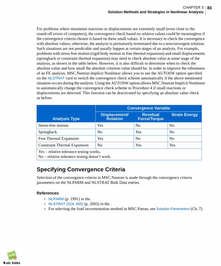
83CHAPTER 3Solution Methods and Strategies in Nonlinear Analysis
For problems where maximum reactions or displacements are extremely small (even close to theround-off errors of computers), the convergence check based on relative values could be meaningless ifthe convergence criteria chosen is based on these small values. It is necessary to check the convergencewith absolute values; otherwise, the analysis is prematurely terminated due to a nonconvergent solution.Such situations are not predicable and usually happen at certain stages of an analysis. For example,problems with stress free motion (rigid body motion or free thermal expansion) and small displacements(springback or constraint thermal expansion) may need to check absolute value at some stage of theanalysis, as shown in the table below. However, it is also difficult to determine when to check theabsolute value and how small the absolute criterion value should be. In order to improve the robustnessof an FE analysis, MSC.Nastran Implicit Nonlinear allows you to use the AUTOSW option specifiedon the NLSTRAT card to switch the convergence check scheme automatically if the above mentionedsituation occurs during the analysis. Using the AUTOSW option allows MSC.Nastran Implicit Nonlinearto automatically change the convergence check scheme to Procedure 4 if small reactions ordisplacements are detected. This function can be deactivated by specifying an absolute value checkas before..
Specifying Convergence CriteriaSelection of the convergence criteria in MSC.Nastran is made through the convergence criteriaparameters on the NLPARM and NLSTRAT Bulk Data entries.
References• NLPARM (p. 1991) in the .• NLSTRAT (SOL 600) (p. 2005) in the .• For selecting the load incrementation method in MSC.Patran, see Solution Parameters (Ch. 7).
Analysis Type
Convergence Variable
Displacement/Rotation
ResidualForce/Torque
Strain Energy
Stress-free motion Yes No No
Springback No Yes No
Free Thermal Expansion Yes No No
Constraint Thermal Expansion No Yes Yes
Yes – relative tolerance testing works.No – relative tolerance testing doesn’t work.

MSC.Nastran 2007 r1 Implicit Nonlinear (SOL 600) User’s Guide84
Singularity RatioThe singularity ratio, , is a measure of the conditioning of the system of linear equations. is related
to the conditioning number, , which is defined as the ratio between the highest and lowest eigenvaluesin the system. The singularity ratio is an upper bound for the inverse of the matrix conditioning number.
(3-65)
and establish the growth of errors in the solution process. If the errors on the right-hand side of the
equation are less than prior to the solution, the errors in the solution will be less than , with
(3-66)
The singularity ratio is a measure that is computed during the Crout elimination process of MSC.NastranImplicit Nonlinear using the direct solver. In this process, a recursive algorithm redefines thediagonal terms
(3-67)
where is a function of the matrix profile. is a diagonal of the kth degree of freedom. The singularity
ratio is defined as
(3-68)
If all and are positive, the singularity ratio indicates loss of accuracy during the Crout
elimination process. This loss of accuracy occurs for all positive definite matrices. The number of digitslost during the elimination process is approximately equal to
(3-69)
The singularity ratio also indicates the presence of rigid body modes in the structure. In that case, the
elimination process produces zeros on the diagonal . Exact zeros never appear because of
numerical error; therefore, the singularity ratio is of the order
(3-70)
where is the accuracy of floating-point numbers used in the calculation. For most versions of
MSC.Nastran Implicit Nonlinear, . If rigid body modes are present, is very small or
negative. If either a zero or a negative diagonal is encountered, execution of MSC.Nastran ImplicitNonlinear is terminated because the matrix is diagnosed as being singular.
R R
C
1 R C≤⁄
C R
E δ
δ CE≤
Kkkk( )
Kkkk 1–( )
Kmk
m i=
k 1–
∑–= Kmk 1 i k 1–≤ ≤
i Kkk
R min Kkkk( )
Kkkk 1–( )⁄=
Kkkk( )
Kkkk 1–( )
nlos t log10R–=
Kkkk( )
0≅
R O 10ndigi t–
=
ndigit
ndigit 12> Kkkk( )

85CHAPTER 3Solution Methods and Strategies in Nonlinear Analysis
You can force the solution of a nonpositive definite or singular matrix. In this case, MSC.Nastran Implicit
Nonlinear does not stop when it encounters a negative or small term on the diagonal. If you use
Lagrangian multiplier elements, the matrix becomes nonpositive definite and MSC.Nastran Implicit
Nonlinear automatically disables the test on the sign of . However, it still tests for singular behavior.
MSC.Nastran SOL 600 also supports the PARAM,AUTOSPC, in which case the rigid body mechanismis suppressed by putting a large number on the diagonal. The value of EPS on the AUTOSPC case controlis set to 1.E-8.
Kkkk( )
Kkkk( )
Note: The correctness of a solution obtained for a linearized set of equations in a nonpositivedefinite system is not guaranteed.

MSC.Nastran 2007 r1 Implicit Nonlinear (SOL 600) User’s Guide86
Guidelines for Analysis Methods
Analysis MethodsNonlinear analysis is usually more complex and expensive than linear analysis. Also, a nonlinearproblem can never be formulated as a set of linear equations. In general, the solutions of nonlinearproblems always require incremental solution schemes and sometimes require iterations (or recycles)within each load/time increment to ensure that equilibrium is satisfied at the end of each step.Superposition cannot be applied in nonlinear problems.
General TipsA nonlinear problem does not always have a unique solution. Sometimes a nonlinear problem does nothave any solution, although the problem can seem to be defined correctly.
• Nonlinear analysis requires good judgment and uses considerable computing time. Several runsare often required. The first run should extract the maximum information with the minimumamount of computing time. Some design considerations for a preliminary analysis are:
• Minimize degrees of freedom whenever possible.
• Always run a linear static analysis to check the model before attempting a nonlinear analysis.
• Impose a coarse tolerance on convergence to reduce the number of iterations. A coarse rundetermines the area of most rapid change where additional load increments might be required.Plan the increment size in the final run by the following rule of thumb: there should be as manyload increments as required to fit the nonlinear results by the same number of straight lines.
MSC.Nastran Implicit Nonlinear solves nonlinear static problems according to one of the following twomethods: tangent modulus or initial strain. Examples of the tangent modulus method are elastic-plasticanalysis, nonlinear springs, nonlinear foundations, large displacement analysis and gaps. This methodrequires at least the following three controls:
• A tolerance on convergence.• A limit to the maximum allowable number of recycles.• Specification of a minimum number of recycles.
An example of the initial strain method is creep or viscoelastic analysis. Creep analysis requires thefollowing tolerance controls:
• Maximum relative creep strain increment control.• Maximum relative stress change control.• A limit to the maximum allowable number of recycles.
Choosing a Solution MethodWhich solution method to use depends very much on the problem. In some cases, one method can beadvantageous over another; in other cases, the converse might be true.

87CHAPTER 3Solution Methods and Strategies in Nonlinear Analysis
The four iterative procedures available in MSC.Nastran Implicit Nonlinear are: Newton-Raphson,Modified Newton-Raphson, Newton-Raphson with strain correction modification, and aSecant procedure.
For Static analysis, MSC.Nastran Implicit Nonlinear uses the Newton-Raphson method as the default forsolving the nonlinear equilibrium equations. The motivation for this choice is primarily the convergencerate obtained by using Newton’s method compared to the convergence rates obtained by alternatemethods (modified Newton or quasi-Newton methods) for the types of nonlinear problems most oftenstudied by MSC.Nastran Implicit Nonlinear.
Time Steps or Load IncrementsThe issue of choosing suitable time steps is a difficult problem to resolve. First of all, considerations arequite different in static, dynamic, and heat transfer cases. It is always necessary to model the response asa function of time to some acceptable level of accuracy. In the case of dynamic or heat transfer problems,time is a physical dimension for the problem, and the time-stepping scheme must provide suitable stepsto allow accurate modeling in this dimension. Even if the problem is linear, this accuracy requirementimposes restrictions on the choice of the time step. In contrast, most static problems have no imposedtime scale, and the only criterion involved in time step choice is accuracy involved in modeling nonlineareffects. In dynamic and heat transfer problems, it is exceptional to encounter discontinuities in the timehistory, because inertia and viscous effects provide smoothing in the solution (an exception is impact).However, in static cases, sharp discontinuities (such as bifurcation caused by buckling) are common.Softening systems or unconstrained systems require special attention in static cases, but are handlednaturally in static or heat transfer cases. Thus, the consideration upon which time step choice is made arequite different for the three problem classes.
MSC.Nastran Implicit Nonlinear provides both fixed and automatic time step choice. Fixed timestepping is useful in cases where the problem behavior is well understood (as might occur when the useris carrying out a series of parameter studies), or in cases where the automatic algorithms do not handlethe problem well. However, the automatic schemes in MSC.Nastran Implicit Nonlinear are based onextensive experience with a wide range of problems, and therefore generally provide a reliable approach.
A fixed-time stepping approach avoids some convergence problems with AUTO LOAD particularly formultiple subcases. AUTO LOAD is still available but the new approach is recommended particularly formultiple subcases. The available methods are selected using PARAM,MARCITER,N where N is thenumber of fixed time steps desired.
For static problems, MSC.Nastran Implicit Nonlinear uses a scheme based predominantly on themaximum force residuals following each iteration. By comparing consecutive values of these quantities,MSC.Nastran Implicit Nonlinear determines whether convergence is likely in a reasonable number ofiterations. If convergence is deemed unlikely, MSC.Nastran Implicit Nonlinear adjusts the loadincrement; otherwise MSC.Nastran Implicit Nonlinear continues with the iteration process. In this way,excessive iteration is eliminated in cases, where convergence is unlikely, and an increment that appearsto be converging is not aborted due to its needing a few more iterations. One other ingredient in thisalgorithm is that a minimum increment size is specified. This prevents excessive computation in cases

MSC.Nastran 2007 r1 Implicit Nonlinear (SOL 600) User’s Guide88
where buckling, limit load, or some modeling error causes the problem to stall. Other controls are builtinto the algorithm, for example, it will cut back the increment size if an element inverts due to excessivelylarge geometry changes.
Nonlinear DynamicsIn dynamic analysis when implicit integration is used, the automatic time stepping is based on theconcept of half-step residuals. The basic idea is that the time-stepping operator defines the velocities andaccelerations at the end of the step in terms of displacement at the end of the step and conditions at thebeginning of the step. Equilibrium is then established at the end of the step. This, then ensures anequilibrium solution at the end of each time step, and thus, at the beginning and end of any individualtime step. However, these equilibrium solutions do not guarantee equilibrium throughout the step. Thetime-step control is based on measuring the equilibrium error (the force residuals) at some point duringthe time step, by using the integrator operator together with the solution obtained at the end of the step,to interpolate within a time step. This evaluation is performed at the half step. If the maximum entry inthis residual vector (the maximum “half step” residual) is greater than a user-specified tolerance, the timestep is considered too big and is replaced by an appropriate factor. If the maximum half-step residual issufficiently below the user-specified tolerance, the time step may be increased by an appropriate factorfor the next increment. Otherwise, the time step is deemed adequate.
MSC.Nastran Implicit Nonlinear is designed to analyze structural components, by which is meant thatthe overall dynamic response of a structure is sought, in contrast to wave propagation solutions associatedwith relatively local response in continua. These are labelled “inertial problems”, classified as problemsin which “wave effects such as focusing, reflection, and diffraction are not important.” Structuralproblems are considered “inertial” because the response time sought is long compared to the timerequired for waves to traverse the structure. The equilibrium considerations are similar to those fornonlinear statics.
Buckling
In problems which are linear until buckling occurs, due to a sudden development of nonlinearity, it issometimes necessary for you to guide the arc-length algorithm by making sure that the arc length remainssufficiently small prior to the occurrence of buckling.
EfficiencyEven if a solution is obtainable, there is always the issue of efficiency. The pros and cons of each solutionprocedure, in terms of matrix operations and storage requirements have been discussed in the previoussections. A very important variable regarding overall efficiency is the size of the problem. The timerequired to assemble a stiffness matrix, as well as the time required to recover stresses after a solution,vary roughly linearly with the number of degrees of freedom of the problem. On the other hand, the timerequired to go through the solver when using the direct method varies roughly quadratically with thebandwidth, as well as linearly with the number of degrees of freedom.

89CHAPTER 3Solution Methods and Strategies in Nonlinear Analysis
In small problems, where the time spent in the solver is negligible, you can easily wipe out any solvergains, or even of assembly gains, with solution procedures such as a line search which requires adouble stress recovery. Also, for problems with strong material or contact nonlinearities, gainsobtained in assembly in modified Newton-Raphson can be nullified by increased number of iterationsor nonconvergence.
References1. Zienkiewicz, O. C. and R. L. Taylor. The Finite Element Method (4th ed.) Vol. 1. Basic
Formulation and Linear Problems (1989),) Vol. 2. Solid and Fluid Mechanics, Dynamics, andNonlinearity (1991) McGraw-Hill Book Co., London, U. K.
2. Bathe, K. J. Finite Element Procedures, Prentice-Hall, Englewood Cliffs, NJ, 1995.
3. Hughes, T. J. R. The Finite Element Method–Linear Static and Dynamic Finite Element Analysis,Prentice-Hall, Englewood Cliffs, NJ. 1987.
4. Ogden, R. W. “Large Deformation Isotropic Elasticity: On The Correlation of Theory andExperiment for Incompressible Rubberlike Solids,” Proceedings of the Royal Society, Vol. A(326), pp. 565-584, 1972.
5. Cook, R. D., D. S. Malkus, and M. E. Plesha, Concepts and Applications of Finite ElementAnalysis (3rd ed.), John Wiley & Sons, New York, NY, 1989.
6. Bathe, K. J. Finite Element Procedures, Prentice Hall, Englewood Cliffs, NJ, 1996.
7. Riks, E. “An incremental approach to the solution of solution and buckling problems”, Int. J. ofSolids and Structures, V. 15, 1979.
8. Riks, E. “Some Computational Aspects of the Stability Analysis of Nonlinear Structures”, Comp.Methods in Appl. Mech. and Eng., 47, 1984.
9. Crisfield, M. A. “A fast incremental iterative procedure that handles snapthrough”, Comput. &Structures, V. 13, 1981.
10. Ramm, E. “Strategies for tracing the nonlinear response near limit points,” in K. J. Bathe et al(eds), Europe-US Workshop on Nonlinear Finite Element Analysis in Structural Mechanics,Ruhr University Bochum, Germany, Springer-Verlag, Berlin, pp/ 63-89. Berlin, 1985.

MSC.Nastran 2007 r1 Implicit Nonlinear (SOL 600) User’s Guide90

MSC.Nastran 2005 r3 Implicit Nonlinear (SOL 600) User’s GuideCh. 4: Nonlinearity and Analysis Types
4 Nonlinearity and Analysis Types
Linear and Nonlinear Analysis 92
Nonlinear Effects and Formulations 93
Overview of Analysis Types 116
Static Analysis 118
Body Approach 120
Buckling Analysis 121
Normal Modes 124
Transient Dynamic Analysis 132
Creep 140

MSC.Nastran 2007 r1 Implicit Nonlinear (SOL 600) User’s Guide92
Linear and Nonlinear AnalysisIn a linear static analysis we implicitly assume that the deflections and strains are very small and thestresses are smaller than the material yield stresses. Consequently, the stiffness can be considered toremain constant (i.e., independent of the displacements and forces) and the finite element equilibriumequations
are linear. Where the stiffness matrix is independent of both , the generalized displacement vector,
and , the generalized force vector. This linearity implies that any increase or decrease in the load willproduce proportional increase or decrease in displacements, strains and stresses. Linear static problemsare solved in one step-a single decomposition of the stiffness matrix.
However, we know that in many structures the deflections and the stresses do not change proportionatelywith the loads. In these problems the structure’s response depends upon its current state and theequilibrium equations reflect the fact that the stiffness of the structure is dependent on both and .
As the structure displaces due to loading, the stiffness changes, and as the stiffness changes the structure’sresponse changes. As a result, nonlinear problems require incremental solution schemes that divide theproblem up into steps calculating the displacement, then updating the stiffness. Each step uses the resultsfrom the previous step as a starting point. As a result the stiffness matrix must be generated and invertedmany times during the analysis adding time and costs to the analysis.
Linear AnalysisSOL 600 allows you to perform linear elastic analysis using any element type in the program. Variouskinematic constraints and loadings can be prescribed to the structure being analyzed; the problem caninclude both isotropic and anisotropic elastic materials.
The principle of superposition holds under conditions of linearity. Therefore, several individual solutionscan be superimposed (summed) to obtain a total solution to a problem.
Linear analysis does not require storing as many quantities as does nonlinear analysis; therefore, it usesthe core memory more sparingly. The assembled and decomposed stiffness matrices can be reused toarrive at repeated solutions for different loads.
Nonlinear AnalysisNonlinear analysis, while most complex and expensive, must be used to establish accurate results whena structure is subject to large deformations, when the material behavior falls outside of a linear elasticmodel, or where the structural interactions include contact.
In nonlinear analysis the stiffness matrix is assembled and decomposed repeatedly throughout theincrementation process. This adds considerable time and cost to the analysis. In addition, because theresponse is not proportional to the loads, each load case must be solved separately and the principle ofsuperposition is not applicable.
P Ku=
K u
P
u P
P K P u,( )u=

93CHAPTER 4Nonlinearity and Analysis Types
Nonlinear Effects and FormulationsThere are three sources of nonlinearity: material, geometric, and nonlinear boundary conditions.Material nonlinearity results from the nonlinear relationship between stresses and strains. Considerableprogress has been made in attempts to derive the continuum or macroscopic behavior of materials frommicroscopic backgrounds, but, up to now, commonly accepted constitutive laws are phenomenological.Difficulty in obtaining experimental data is usually a stumbling block in mathematical modeling ofmaterial behavior. A plethora of models exist for more commonly available materials like elastomers andmetals. Other material model of considerable practical importance are: composites, viscoplastics, creep,soils, concrete, powder, and foams. Figure 4-1 shows the elastoplastic, elasto-viscoplasticity, and creep.Although the situation of strain hardening is more commonly encountered, strain softening andlocalization has gained considerable importance in recent times.
Geometric nonlinearity results from the nonlinear relationship between strains and displacements on theone hand and the nonlinear relation between stresses and forces on the other hand. If the stress measureis conjugate to the strain measure, both sources of nonlinearity have the same form. This type ofnonlinearity is mathematically well defined, but often difficult to treat numerically. Two important typesof geometric nonlinearity occur:
1. The analysis of buckling and snap-through problems (see Figure 4-2 and Figure 4-3).
2. Large strain problems such as manufacturing, crash, and impact problems. In such problems, dueto large strain kinematics, the mathematical separation into geometric and material nonlinearityis nonunique.
Figure 4-1 Material Nonlinearity
σ
εElasto-Plastic Behavior
σ
εElasto-Viscoplastic Behavior
ε
εc
tCreep Behavior
σ

MSC.Nastran 2007 r1 Implicit Nonlinear (SOL 600) User’s Guide94
Figure 4-2 Buckling
Figure 4-3 Snap-Through
Boundary conditions and/or loads can also cause nonlinearity. Contact and friction problems lead tononlinear boundary conditions. This type of nonlinearity manifests itself in several real life situations;for example, metal forming, gears, interference of mechanical components, pneumatic tire contact, andcrash (see Figure 4-4). Loads on a structure cause nonlinearity if they vary with the displacements of thestructure. These loads can be conservative, as in the case of a centrifugal force field (see Figure 4-5); theycan also be nonconservative, as in the case of a follower force on a cantilever beam (see Figure 4-6). Also,such a follower force can be locally nonconservative, but represent a conservative loading system whenintegrated over the structure. A pressurized cylinder (see Figure 4-7) is an example of this.
Figure 4-4 Contact and Friction Problem
P
u
Linear
Stable
Neutral
Unstable
P
Pc
u
P
u
P
u

95CHAPTER 4Nonlinearity and Analysis Types
Figure 4-5 Centrifugal Load Problem (Conservative)
Figure 4-6 Follower Force Problem (Nonconservative)
Figure 4-7 Pressurized Cylinder (Globally Conservative)
The three types of nonlinearities are described in detail in the following sections.
P
P

MSC.Nastran 2007 r1 Implicit Nonlinear (SOL 600) User’s Guide96
Geometric NonlinearitiesGeometric nonlinearity leads to two types of phenomena: change in structural behavior and loss ofstructural stability.
There are two natural classes of large deformation problems: the large displacement, small strain problemand the large displacement, large strain problem. For the large displacement, small strain problem,changes in the stress-strain law can be neglected, but the contributions from the nonlinear terms in thestrain displacement relations cannot be neglected. For the large displacement, large strain problem, theconstitutive relation must be defined in the correct frame of reference and is transformed from this frameof reference to the one in which the equilibrium equations are written.
The collapse load of a structure can be predicted by performing an eigenvalue analysis. If performed afterthe linear solution (increment zero), the Euler buckling estimate is obtained. An eigenvalue problem canbe formulated after each increment of load; this procedure can be considered a nonlinear bucklinganalysis even though a linearized eigenvalue analysis is used at each stage.
The kinematics of deformation can be described by the following approaches:
• Lagrangian Formulation• Eularian Formulation
The choice of one over another can be dictated by the convenience of modeling physics of the problem,rezoning requirements, and integration of constitutive equations, and can be specified usingPARAM,MARUPDAT.
Lagrangian Formulation
In the Lagrangian method, the finite element mesh is attached to the material and moves through spacealong with the material. In this case, there is no difficulty in establishing stress or strain histories at aparticular material point and the treatment of free surfaces is natural and straightforward.
The Lagrangian approach also naturally describes the deformation of structural elements; that is, shellsand beams, and transient problems, such as the indentation problem shown in Figure 4-8.
Figure 4-8 Indentation Problem with Pressure Distribution on Tool
sz
∆u

97CHAPTER 4Nonlinearity and Analysis Types
This method can also analyze steady-state processes such as extrusion and rolling. Shortcomings of theLagrangian method are that flow problems are difficult to model and that the mesh distortion is as severeas the deformation of the object. Severe mesh degeneration is shown in Figure 4-9b. However, recentadvances in adaptive meshing and rezoning available in MSC.Marc have alleviated the problems ofpremature termination of the analysis due to mesh distortions as shown in Figure 4-9c.
Figure 4-9 Rezoning Example
The Lagrangian approach can be classified in two categories: the total Lagrangian method and theupdated Lagrangian method. In the total Lagrangian approach, the equilibrium is expressed with theoriginal undeformed state as the reference; in the updated Lagrangian approach, the currentconfiguration acts as the reference state. The kinematics of deformation and the description of motion isgiven in Table 4-1 and Figure 4-10.
Table 4-1 Kinematics and Stress-Strain Measures in Large Deformation
Configuration Measures Reference (t = 0 or n) Current (t = n + 1)
Coordinates X x
Deformation Tensor C (Right Cauchy-Green) b (Left Cauchy-Green)
Strain Measure E (Green-Lagrange)F (Deformation Gradient)
e (Logarithmic)
Stress Measure S (second Piola-Kirchhoff)P (first Piola-Kirchhoff)
σ (Cauchy)
(a) Original (b) Deformed Mesh(Undeformed Mesh) Before Rezoning
(c) Deformed MeshAfter Rezoning

MSC.Nastran 2007 r1 Implicit Nonlinear (SOL 600) User’s Guide98
Figure 4-10 Description of Motion
Total Lagrangian Procedure
The total Lagrangian procedure can be used for linear or nonlinear materials, in conjunction with staticor dynamic analysis. Although this formulation is based on the initial element geometry, the incrementalstiffness matrices are formed to account for previously developed stress and changes in geometry.
This method is particularly suitable for the analysis of nonlinear elastic problems (for instance, with theMooney or Ogden material model). The total Lagrangian approach is also useful for problems inplasticity and creep, where moderately large rotations but small strains occur. A case typical in problemsof beam or shell bending. However, this is only due to the approximations involved.
In the total Lagrangian approach, the equilibrium can be expressed by the principle of virtual work as:
(4-1)
Here is the symmetric second Piola-Kirchhoff stress tensor, , is the Green-Lagrange strain, is
the body force in the reference configuration, is the traction vector in the reference configuration, and
is the virtual displacements. Integrations are carried out in the original configuration at . The
strains are decomposed in total strains for equilibrated configurations and the incremental strainsbetween and as:
(4-2)
Reference
t = 0
Current
t = n + 1
Previous
t = n
un + 1
F
f
∆u
Fn
un
Fn+1 = Fn
SijδEij VdV0
∫ bi0 δηi V ti
0 δηi AdA0
∫+dV0
∫=
Sij Eij bi0
ti0
ηi t 0=
t n= t n 1+=
Eijn 1+
Eijn
∆Eij+=

99CHAPTER 4Nonlinearity and Analysis Types
while the incremental strains are further decomposed into linear, and nonlinear, parts as:
where is the linear part of the incremental strain expressed as:
(4-3)
The second term in the bracket in Equation (4-3) is the initial displacement effect. is the nonlinearpart of the incremental strain expressed as:
(4-4)
Linearization of equilibrium of Equation (4-1) yields:
(4-5)
where is the small displacement stiffness matrix defined as
is the initial displacement stiffness matrix defined as
in the above equations, and are the constant and displacement dependent symmetric shape
function gradient matrices, respectively, and is the material tangent,
and is the initial stress stiffness matrix
in which is the second Piola-Kirchhoff stresses and is the shape function gradient matrix.
∆Eij ∆Eijn
∆Eij ∆Eij ∆Enij+=
∆E
∆E12---
∂∆ui
∂Xj------------
∂∆uj
∂Xi------------+
12---
∂ukn
∂Xi--------- ∂∆uk
∂Xj------------- +=
∆En
∆En 1
2---
∂∆uk
∂Xi------------- ∂∆uk
∂Xj------------- ∂uk
n
∂Xj--------- ∂∆uk
∂Xi------------- +=
K0 K1 K2+ +{ }δu F R–=
K0
K0( )i j
βimn0
Dmnpqβpqj0
VdV0
∫=
K1
K1( )i j
βimnu
Dmnpqβpqju βimn
uDmnpqβpqj
0 βimnu
Dmnpqβpqju
+ +{ } VdV0
∫=
βimn0 βimn
u
Dmnpq
K2
K2( )i j
Ni k, Nj l, Skl VdV0
∫=
Skl Ni k,

MSC.Nastran 2007 r1 Implicit Nonlinear (SOL 600) User’s Guide100
Also, is the correction displacement vector. and are the external and internalforces, respectively.
This Lagrangian formulation can be applied to problems if the undeformed configuration is known sothat integrals can be evaluated, and if the second Piola-Kirchhoff stress is a known function of the strain.The first condition is not usually met for fluids, because the deformation history is usually unknown. Forsolids, however, each analysis usually starts in the stress-free undeformed state, and the integrations canbe carried out without any difficulty.
For viscoelastic fluids and elastic-plastic and viscoplastic solids, the constitutive equations usuallysupply an expression for the rate of stress in terms of deformation rate, stress, deformation, andsometimes other (internal) material parameters. The relevant quantity for the constitutive equations is therate of stress at a given material point.
It, therefore, seems most obvious to differentiate the Lagrangian virtual work equation with respect totime. The rate of virtual work is readily found as
(4-6)
This formulation is adequate for most materials, because the rate of the second Piola-Kirchhoff stress canbe written as
(4-7)
For many materials, the stress rate is even a linear function of the strain rate
(4-8)
Equation (4-6) supplies a set of linear relations in terms of the velocity field. The velocity field can besolved noniteratively and the displacement can be obtained by time integration of the velocities.
The second Piola-Kirchhoff stress for elastic and hyperelastic materials is a function of the Green-Lagrange strain defined below:
(4-9)
If the stress is a linear function of the strain (linear elasticity)
(4-10)
the resulting set of equations is still nonlinear because the strain is a nonlinear function of displacement.
δu F R
S·i j
δEij Sij
∂vk
∂Xi---------
∂δηk
∂Xj-------------+ dV
V0
∫ b·iδηidV t
·iδηidA
A0
∫+V0
∫=
S·i j S
·i j E
·kl Smn Epq, ,( )=
S·i j Dijk l Smn Epq,( )E
·kl=
Sij Sij Ekl( )=
Sij DijklEkl=

101CHAPTER 4Nonlinearity and Analysis Types
Updated Lagrangian Procedure
The updated Lagrange formulation takes the reference configuration at . True or Cauchystress and an energetically conjugate strain measure, namely the true strain, are used in the constitutiverelationship.
The updated Lagrangian approach is useful in:
• analysis of shell and beam structures in which rotations are large so that the nonlinear terms inthe curvature expressions may no longer be neglected, and
• large strain plasticity analysis, for calculations which the plastic deformations cannot beassumed to be infinitesimal.
In general, this approach can be used to analyze structures where inelastic behavior (for example,plasticity, viscoplasticity, or creep) causes the large deformations. The (initial) Lagrangian coordinateframe has little physical significance in these analyses since the inelastic deformations are, by definition,permanent. For these analyses, the Lagrangian frame of reference is redefined at the last completediteration of the current increment.
It is instructive to derive the stiffness matrices for the updated Lagrangian formulation starting from thevirtual work principle in Equation (4-9).
Direct linearization of the left-hand side of Equation (4-9) yields:
(4-11)
where ∆u and η are actual incremental and virtual displacements respectively, and σkj is Cauchy stresstensor.
(4-12)
denotes the symmetric part of , which represents the gradient operator in the current configuration.Also, in Equation (4-11) and Equation (4-12), three identities are used:
t n 1+=
Sij δEij( )d( ) VdV0
∫ ∇ηikσkj∇∆uij
vdVn 1+
∫=
SijδEijd VdV0
∫ ∇sηi jLi jk l∇s ∆ukl( ) vd
Vn 1+
∫=
∇s ∇

MSC.Nastran 2007 r1 Implicit Nonlinear (SOL 600) User’s Guide102
(4-13)
in which represents the material moduli tensor in the reference configuration which is convected
to the current configuration, . This yields:
(4-14)
where is the material stiffness matrix written as
in which is the symmetric gradient operator-evaluated in the current configuration and is the
Cauchy stresses
and is the geometric stiffness matrix written as
while and are the external and internal forces, respectively.
Keeping in view that the reference state is the current state, a rate formulation analogous to Equation (4-6)can be obtained by setting:
(4-15)
where F is the deformation tensor, and d is the rate of deformation. Hence,
(4-16)
σi j1J---FimSmnFjn=
δEij Fmi∇sηmnFnj=
Lijkl1J---FimFjnFkpFlqDmnpq=
and
Dmnpq
Lijk
K1 K2+{ }δu F R–=
K1
K1( )i j
βimnLmnpqβpqjVn 1+
∫=
βimn σkl
K2
K2( )i j
σklNi k, Nj l, vdVn 1+
∫=
F R
Fij δi j δEij, δdi j∂
∂Xi---------, ∂
∂xi-------- Sij, σi j= = = =
∇σi jδdij σi j
∂vk
∂xi---------
∂δηk
∂xj-------------+ dv
Vn 1+
∫ b· iδηidvVn 1+
∫ t·iδηidaAn 1+
∫+=

103CHAPTER 4Nonlinearity and Analysis Types
in which and is the body force and surface traction, respectively, in the current configuration
In this equation, is the Truesdell rate of Cauchy stress which is essentially a Lie derivative of Cauchy
stress obtained as:
(4-17)
The Truesdell rate of Cauchy stress is materially objective implying that if a rigid rotation is imposed onthe material, the Truesdell rate vanishes, whereas the usual material rate does not vanish. This fact hasimportant consequences in the large deformation problems where large rotations are involved. Theconstitutive equations can be formulated in terms of the Truesdell rate of Cauchy stress as:
Specifying the Geometric Nonlinearity Formulation
Selection of the geometric nonlinearity formulation in MSC.Nastran is made on the MARUPDATparameter entry.
References• MARUPDAT(p. 723) in the .
• For selecting the geometric nonlinearity formulation in MSC.Patran, see Subcase Parameters(Chapter 7).
More on Using Total Lagrangian
MSC.Nastran Implicit Nonlinear will normally determine whether Total Lagrangian or UpdatedLagrangian is best for a particular problem. If you wish to exert more control, the parameters discussedin this section and the next may be employed.
For problems (such as centrifugal or pressure load) that require follower forces, use the LGDISPparameter. This parameter forms all distributed loads on the basis of the current geometry.
• LGDISP(p. 682) in the .
bi ti
∇σi j
σi j∇
Fin JFnk
1–σklFml
1–( )
·= Fmj
∇σi j Li jk dk=
Note: Depending on the type of analysis specified by all entries in the input deck,PARAMETER,MARUPDAT will be specified automatically as -1 or 1 unless entered bythe user.

MSC.Nastran 2007 r1 Implicit Nonlinear (SOL 600) User’s Guide104
Using only the LGSTRN, 2 parameter, MSC.Nastran Implicit Nonlinear uses the total Lagrangianmethod. When the total Lagrangian method is specified, the program uses and prints second Piola-Kirchhoff stress and Green-Lagrange strain. These measures are suitable for analysis with largeincremental rotations and large incremental strains.
More on Using Updated Lagrangian
You can use the updated procedure with or without MSC.Nastran’s LGDISP parameter. When you usethe LGDISP parameter, MSC.Nastran Implicit Nonlinear takes into account the effect of the internalstresses by forming the initial stress stiffness. MSC.Nastran Implicit Nonlinear also calculates the strainincrement to second order accuracy to allow large rotation increments.
Another option is to use the MARUPDAT parameter (with or without the LGDISP parameter) to definea new (Lagrangian) frame of reference at the beginning of each increment. This option is suitable foranalysis of problems of large total rotation but small strain. If analysis of large plastic strain is required,use PARAM,MRFINITE,1 in addition to the PARAM, MARUPDAT parameter in which caseMSC.Nastran Implicit
With MARUPDAT,1 MSC.Nastran Implicit Nonlinear uses Cauchy stresses and true strains. Thiscombination of parameters is suitable for analyses with small incremental rotations and smallincremental strains. Stress and strain components are printed with respect to the current state.
The MSC.Marc plasticity parameter with options 3 or 5 utilize the updated Lagrange procedure forelastic-plastic analysis. The MSC.Marc,elasticity parameter with option 2 utilizes the updated Lagrangeprocedure for large strain elasticity (Mooney or Ogden).
The combination of PARAM,MARUPDAT,1 and PARAM,MARCDILT (i.e., with constant dilatation) ora MATEP material entry results in a complete large strain plasticity formulation (with B-Bar method) tosatisfy incompatibility using the updated Lagrange procedure. The use of MATEP replaces the need ofthe MARCDILT parameter. The program internally uses true (Cauchy) stress and rotation neutralizedstrains. In the case of proportional straining, this method leads to logarithmic strains.
Note: Do not use MSC.Marc’s CENTROID parameter with this parameter. Always use residualload corrections with this parameter. To input control tolerances for large displacementanalysis, use model definition option NLSTRAT.
Note: For materials exhibiting large strain plasticity with volumetric changes (for example, soils,powder, snow, wood) only MSC.Marc’s LARGE DISP, FINITE and UPDATE should beused (these are created automatically for you by the internal MSC.Marc translator inMSC.Nastran). Use of MARCDILT parameter or MATEP will enforce theincompressibility condition and, in such materials, yield incorrect and nonphysicalbehavior.

105CHAPTER 4Nonlinearity and Analysis Types
Large strain rubber elasticity can be modeled in either total Lagrange MSC.Nastran’sPARAM,MARCUPDAT,1: second Piola-Kirchhoff stress, Green Lagrange strain or updated LagrangePARAM,MARCELAS,2: Cauchy stress, Logarithmic strain framework.
Theoretically and numerically, if formulated mathematically correct, the two formulations yield exactlythe same results. However, integration of constitutive equations for certain types of material behavior(for example, plasticity) make the implementation of the total Lagrange formulation inconvenient. If theconstitutive equations are convected back to the original configuration and proper transformations areapplied, then both formulations are equivalent.
Options Kinematics Formulation
param,marcplas,1 Total Lagrange Small strain, mean normal, additive decomposition ofstrain rates.
param,marcplas,3
default
Updated Lagrange Large strain, mean normal, additive decomposition ofstrain rates.
param,marcplas,5 Updated Lagrange Large strain, radial return multiplicative decomposition ofdeformation gradient.
param,marcelas,1 Total Lagrange Large strain.
param,marcelas,2 Updated Lagrange Large strain.

MSC.Nastran 2007 r1 Implicit Nonlinear (SOL 600) User’s Guide106
Material NonlinearitiesIn a large strain analysis, it is usually difficult to separate the kinematics from the material description.The following table lists the characteristics of some common materials.
A complete description of the material types mentioned in the table is given in Materials (Chapter 10).However, some notable characteristics and procedural considerations of some commonly encounteredmaterials behavior are listed next.
Material Characteristics Examples Models
Composites Anisotropic:
1) layered,21 constants
2)Fiber reinforced,
one-dimensional strain in fibers
Bearings, aircraftpanels
Tires, glass/epoxy
Compositecontinuum elements
Rebars
Creep Strains increasing with time underconstant load.Stresses decreasing with time underconstant deformations.Creep strains are non-instantaneous.
Metals at hightemperatures,polymide films
ORNLNortonMaxwell
Elastic Stress functions of instantaneous strainonly. Linear load-displacementrelation.
Small deformation(below yield) formost materials:metals, glass, wood
Hookes Law
Elasto-plasticity
Yield condition flow rule andhardening rule necessary to calculatestress, plastic strain. Permanentdeformation upon unloading.
MetalsSoils
von Mises IsotropicCam -ClayHill’s Anisotropic
Hyperelastic Stress function of instantaneous strain.Nonlinear load-displacement relation.Unloading path same as loading.
Rubber MooneyOgdenArruda BoyceGentFoam
Hypoelastic Rate form of stress-strain law Concrete NLELAST
Viscoelastic Time dependence of stresses in elasticmaterial under loads. Full recoveryafter unloading.
RubberGlass
Simo ModelNarayanaswamy
Viscoplastic Combined plasticity and creepphenomenon
MetalsPowder
Power lawShima Model
dsij Cijk dεk=
SE2--- T
tCT 1–( )=

107CHAPTER 4Nonlinearity and Analysis Types
Inaccuracies in experimental data, misinterpretation of material model parameters and errors in user-defined material law are some common sources of error in the analysis from the materials viewpoint. Itis useful to check the material behavior by running a small model with prescribed displacement and loadboundary conditions in uniaxial tension and shear (single element tests are not recommended).
Elasticity
Structures composed of elastomers, such as tires and bushings, are typically subjected to largedeformation and large strain. An elastomer is a polymer, such as rubber, which shows a nonlinear elasticstress-strain behavior. The large strain elasticity capability in MSC.Nastran Implicit Nonlinear dealsprimarily with elastomeric materials. These materials are characterized by the form of their elastic strainenergy function.
For the finite element analysis of elastomers, there are some special considerations that do not apply forlinear elastic analysis. These considerations include:
• Mesh Distortion
• Incompressible Behavior
• Instabilities
• Existence of Multiple Solutions
Mesh Distortions
When extremely large deformations occur, the element mesh should be designed so that it can followthese deformations without complete degeneration of elements. This problem is more prevalent when theupdated Lagrange procedure is used. For problems involving extreme distortions, the MSC.Marc globaladaptive remeshing capability should be used.
Incompressible Behavior
One of the most frequent causes of problems analyzing elastomers is the incompressible materialbehavior. Lagrangian multipliers (pressure variables) are used to apply the incompressibility constraint.The result is that the volume is kept constant in a generalized sense, over an element.
Both the total, as well as updated Lagrange formulations, are implemented with appropriate constraintratios for lower- and higher-order elements in 2D and 3D. For many practical analysis, the LBB(Ladyszhenskaya-Babuska-Brezzi) condition does not have to be satisfied in the strictest sense; forexample, four node quadrilateral based on Herrmann principle.
For elements that satisfy the LBB condition, error estimates of the following form can be established
(4-18)
where and are the orders of displacements and pressure interpolations, respectively. If
, the rate of convergence is said to be optimal, and elements satisfying the LBBcondition will not lock.
uh
u– 1 ph
p– 0+ O hmin k 1+,{ }( )=
k
K min k 1+,{ }=

MSC.Nastran 2007 r1 Implicit Nonlinear (SOL 600) User’s Guide108
The large strain elasticity formulation may also be used with conventional plane stress, membrane, andshell elements. Because of the plane stress conditions, the incompressibility constraint can be satisfiedwithout the use of Lagrange multipliers.
Instabilities
Under some circumstances, materials can become unstable. This instability can be real or can be due tothe mathematical formulation used in the calculations.
Instability can also result from the approximate satisfaction of incompressibility constraints. If thenumber of Lagrangian multipliers is insufficient, local volume changes can occur. Under somecircumstances, these volume changes can be associated with a decrease in total energy. This type ofinstability usually occurs only if there is a large tensile hydrostatic stress. Similarly, overconstraints giverise to mesh locking and inordinate increase in total energy under large compressive stresses.
Existence of Multiple Solutions
It is possible that more than one stable solution exists (due to nonlinearity) for a given set of boundaryconditions. An example of such multiple solutions is a hollow hemisphere with zero prescribed loads.Two equilibrium solutions exist: the undeformed stress-free state and the inverted self-equilibrating state.An example of these solutions is shown in Figure 4-11 and Figure 4-12. If the equilibrium solution remainsstable, no problems should occur; however, if the equilibrium becomes unstable at some point in theanalysis, problems can occur.
Figure 4-11 Rubber Hemisphere
y
x

109CHAPTER 4Nonlinearity and Analysis Types
Figure 4-12 Inverted Rubber Hemisphere
When incompressible material is being modeled, the basic linearized incremental procedure is used inconjunction with mixed variational principles similar in form to the Herrmann incompressible elasticformulation. These formulations are incorporated in plane strain, axisymmetric, and three-dimensionalelements. These mixed elements may be used in combination with other elements in the library (suitableconstraint equations may be necessary) and with each other. Where different materials are joined, thepressure variable at the corner nodes must be uncoupled to allow for mean pressure discontinuity. MPC’smust be used to couple the displacements only.
Plasticity
In recent years there has been a tremendous growth in the analysis of metal forming problems by thefinite element method. Although an Eularian flow-type approach has been used for steady-state andtransient problems, the updated Lagrangian procedure, pioneered by McMeeking and Rice, is mostsuitable for analysis of large strain plasticity problems. The main reasons for this are: (a) its ability totrace free boundaries, and (b) the flexibility of taking elasticity and history effects into account. Also,residual stresses can be accurately calculated.
The large strain plasticity capability in MSC.Nastran Implicit Nonlinear allows you to analyze problemsof large-strain, elastic-plastic material behavior. These problems can include manufacturing processessuch as forging, upsetting, extension or deep drawing, and/or large deformation of structures that occurduring plastic collapse. The analysis involves both material, geometric and boundary nonlinearities.
In addition to the options required for plasticity analysis, the PARAM,LGSTRN and/or PARAM,MRTABLS1 parameters are needed for large strain plasticity analysis.
y
x

MSC.Nastran 2007 r1 Implicit Nonlinear (SOL 600) User’s Guide110
In performing finite deformation elastic-plastic analysis, there are some special considerations which donot apply for linear elastic analysis. These considerations include:
• Choice of Finite Element Types
• Nearly Incompressible Behavior
• Treatment of Boundary Conditions
• Severe Mesh Distortion
• Instabilities
Choice of Finite Element Types
Accurate calculation of large strain plasticity problems depends on the selection of adequate finiteelement types. In addition to the usual criteria for selection, two aspects need to be given specialconsideration: the element types selected need to be insensitive to (strong) distortion; for plane strain,axisymmetric, and three-dimensional problems, the element mesh must be able to representnondilatational (incompressible) deformation modes.
Nearly Incompressible Behavior
Most finite element types tend to lock during fully plastic (incompressible) material behavior. A remedyis to introduce a modified variational principle which effectively reduces the number of independentdilatational modes (constraints) in the mesh. This procedure is successful for plasticity problems in theconventional “small” strain formulation. Zienkiewicz pointed out the positive effect of reducedintegration for this type of problem and demonstrates the similarity between modified variationalprocedures and reduced integration. MSC.Software Corporation recommends the use of lower-orderelements, invoking the constant dilatation option with certain exceptions such as 4-node tetras. Thelower-order elements, which use reduced integration and hourglass control, also behave well for nearlyincompressible materials.
Treatment of Boundary Conditions
In many large strain plasticity problems, specifically in the analysis of manufacturing processes, thematerial slides with or without friction over curved surfaces. This results in a severely nonlinearboundary condition. The MSC.Nastran Implicit Nonlinear CONTACT option can model such slidingboundary conditions.
Severe Mesh Distortion
Because the mesh is attached to the deforming material, severe distortion of the element mesh oftenoccurs, which leads to a degeneration of the results in many problems. To avoid this degeneration,generate a new finite element mesh for the problem and then transfer the current deformation state to thenew finite element mesh.

111CHAPTER 4Nonlinearity and Analysis Types
Instabilities
Elastic-plastic structures are sometimes unstable due to necking phenomena. Consider a rod of a rigid-
plastic incompressible workhardening material. With the current true uniaxial strain rate and H the
current workhardening, the rate of true uniaxial stress is equal to
(4-19)
The applied force is equal to , where is the current area of the rod. The rate of the force istherefore equal to
(4-20)
On the other hand, conservation of volume requires that
(4-21)
Hence, the force rate can be calculated as
(4-22)
Instability clearly occurs if . For applied loads (as opposed to applied boundary conditions), thestiffness matrix becomes singular (nonpositive definite).
For the large strain plasticity option, the workhardening slope for plasticity is the rate of true (Cauchy)stress versus the true (logarithmic) plastic strain rate. The workhardening curve must, therefore, beentered as the true stress versus the logarithmic plastic strain in a uniaxial tension test.
Computational Procedures for Elastic-Plastic Analysis
For more information on computational procedures, please see the MSC.Marc Reference manual.
Creep
Creep is a time-dependent inelastic behavior that can occur at any stress level, either below or above theyield stress of a material. Creep is an important factor at elevated temperatures. In many cases, creep isalso accompanied by plasticity, which occurs above the yield stress of the material.
Conventional creep behavior is based on a von Mises creep potential with isotropic behavior describedby the equivalent creep law:
ε·
σ·
σ·
Hε·
=
F σA= A
F·
σ·
A σA·
+=
Aε·
A·
+ 0=
F·
H σ–( )Aε·
=
σ H>
ε· cr
f σ εcr
T t,,,( )=

MSC.Nastran 2007 r1 Implicit Nonlinear (SOL 600) User’s Guide112
The material behavior is therefore described by:
where is the outward normal to the current von Mises stress surface and is the equivalent creep
strain rate.
There are two numerical procedures used in implementing creep behavior. The default is an explicitprocedure in which the above relationship is implemented in the program by an initial strain technique.In other words, a pseudo-load vector due to the creep strain increment is added to the right-hand side ofthe stiffness equation.
where K is the stiffness matrix, and and are incremental displacement and incremental nodalforce vectors, respectively. The integral:
is the pseudo-load vector due to the creep strain increment in which is the strain displacement relation
and is the stress-strain relation. When plasticity is also specified through a suitably defined yieldcriterion and yield stress inMSC.Nastran, the plasticity is treated implicitly while the creep is treatedexplicitly.
As an alternative, an implicit creep procedure can be requested. In this case, the inelastic strain rate hasan influence on the stiffness matrix. Using this technique, significantly larger steps in strain space can beused. This option is only to be used for isotropic materials with the creep strain rate defined by a creepconstant.
∆εcr ε· c r ∂σ
∂σ′--------∆ t=
∂σ
∂σ′-------- ε· cr
K∆u ∆P βT
V∫ D∆εcr
dv+=
∆u ∆P
βT
V∫ D∆εcr
dv
βD

113CHAPTER 4Nonlinearity and Analysis Types
Creep Buckling
MSC.Nastran also predicts the creep time to buckling due to stress redistribution under given load orrepeated cyclic load. The buckling option solves the following equation for the first eigenvalue
(4-23)
The geometric stiffness matrix, , is a function of the increments of stress and displacement. These
increments are calculated during the last creep time step increment. To determine the creep time tobuckle, perform a buckle step after a converged creep increment. Note that the incremental time must bescaled by the calculated eigenvalue, and added to the total (current) time to get an estimate as to whenbuckling occurs.
Viscoelasticity
In certain problems, structural materials exhibit viscoelastic behavior. Two examples of these problemsare quenching of glass and time-dependent deformation of polymeric materials. The viscoelasticmaterial retains linearity between load and deformation; however, this linear relationship depends ontime. Consequently, the current state of deformation must be determined from the entire history ofloading. Different models consisting of elastic elements (spring) and viscous elements (dashpot) can beused to simulate the viscoelastic material behavior described in Materials (Chapter 10). Both the equationof state and the hereditary integral approaches can be used for viscoelastic analysis.
A special class of temperature dependence known as the Thermo-Rheologically Simple behavior (TRS)is also applicable to a variety of thermal viscoelastic problems. To model the thermo-rheologicallysimple material behavior, MATTVE can be used to choose the Williams-Landel-Ferry equation or thepower series expression or Narayanaswamy model.
In MSC.Nastran Implicit Nonlinear, two options are available for small strain viscoelastic analysis. Thefirst option uses the equation of state approach and represents a Kelvin model. The second option isbased on the hereditary integral approach and allows the selection of a generalized Maxwell model. Thethermo-rheologically simple behavior is also available in the second option for thermal viscoelasticanalysis. The Viscoelastic (Chapter 10) discusses these models in detail.
The Simo model for large strain viscoelasticity can be used in conjunction with the damage andhyperelastic Mooney, Ogden, Gent, or Arruda Boyce material model. The large strain viscoelasticmaterial behavior can be simulated by incorporating MATVE.
Nonlinear structural relaxation behavior of materials can be modeled by the Narayanaswamy modelwhich accounts for memory effect. This model allows simulation of evolution of physical properties ofglass subjected to complex time temperature histories. The thermal expansion behavior for theNarayanaswamy model is controlled via the MATTVE bulk data option.
Viscoplasticity
There are two procedures in MSC.Nastran Implicit Nonlinear for viscoplastic analysis: explicit andimplicit. A brief description of each procedure follows:
K λKG+( )φ 0=
KG

MSC.Nastran 2007 r1 Implicit Nonlinear (SOL 600) User’s Guide114
Explicit Method
The elasto-viscoplasticity model in MSC.Nastran Implicit Nonlinear is a modified creep model to whicha plastic element is added. The plastic element is inactive when the stress is less than the yield stress ofthe material. You can use the elasto-viscoplasticity model to solve time-dependent plasticity and creep aswell as plasticity problems with a nonassociated flow law.
The CREEP option in MSC.Nastran Implicit Nonlinear has been modified to enable solving problemswith viscoplasticity. The method is modified to allow solving elastic-plastic problems with nonassociatedflow rules which result in nonsymmetric stress-strain relations if the tangent modulus method is used.
The requirements for solving the viscoplastic problem are:
PARAM,MCREEP,1 and creep controls
Load incrementation immediately followed by a series of creep increments specified byPARAM,MAUTCREP,1.
Use of user subroutine CRPLAW and/or user subroutine NASSOC.
The following load incrementation procedure enables you to solve a viscoplastic problem:
1. Apply an elastic load increment that exceeds the steady-state yield stress.
2. Relieve the high yield stresses by turning on PARAM,MAUTCREP,1.
You may repeat steps 1 and 2 as many times as necessary to achieve the required load history.
The viscoplastic approach converts an iterative elastic-plastic method to one where a fraction of theinitial force vector is applied at each increment with the time step controls. The success of the methoddepends on the proper use of the automatic creep time step controls. This means that it is necessary toselect an initial time step that will satisfy the tolerances placed on the allowable stress change.
The allowable stress change is specified in the creep controls. The most highly stressed element usuallyyields the maximum strain rate. It is also important to select a total time that gives sufficient number ofincrements to work off the effects of the initial force vector. A total time of 30 times the estimated ∆t isusually sufficient.
MSC.Nastran Implicit Nonlinear does not distinguish between viscoplastic and creep strains. A flag isset in the CREEP parameter in order to use the viscoplastic option with a nonassociated flow rule.
The viscoplasticity feature can be used to implement very general constitutive relations with the aid ofuser subroutines ZERO and YIEL.
Since the viscoplasticity model in MSC.Nastran Implicit Nonlinear is a modified creep model, youshould familiarize yourself with the creep analysis procedure (see Creep, Viscoplastic, and ViscoelasticBehavior, page 119 of this chapter).
The initial time step ∆t =allowable stress change x 0.7
Maximum viscoplastic strain rate x Young’s modulus

115CHAPTER 4Nonlinearity and Analysis Types
Implicit Method
A general viscoplastic material law can be implemented through user subroutine UVSCPL. When usingthis method, you are responsible for defining the inelastic strain increment and the current stress.
Nonlinear Boundary ConditionsThere are three types of nonlinear boundary conditions: contact, nonlinear support, and nonlinearloading. The contact problem is solved using the BCONTACT Case Control specification. Nonlinearsupport might involve nonlinear springs and/or foundations. Sometimes nonlinearities due to rigid linksthat become activated or deactivated during an analysis can be modeled through adaptive linearconstraints. Nonlinear loading is present if the loading system is nonconservative, as is the case withfollower forces or frictional slip effects.
Discontinuities are inherent in the nature of many of these nonlinearities, making the solution morechallenging. Some of the most severe nonlinearities in mechanics are introduced by nonlinear boundaryconditions. It is, therefore, very important to be aware of potential problem areas and to have a goodunderstanding of the underlying principles. This awareness and understanding enables you to validatenumerical answers and to take alternative approaches if an initial attempt fails.
Nonlinear Loading
When the structure is deformed, the directions and the areas of the surface loads are changed. For mostdeformed structures, such changes are so small that the effect on the equilibrium equation can be ignored.For some structures, such as flexible shell structure with large pressure loads, the effects on the resultscan be quite significant so that the surface load effects have to be included in the finite element equations.
MSC.Nastran Implicit Nonlinear forms both pressure stiffness and pressure terms based on currentdeformed configuration with MSC.Nastran’s PARAM,LGDISP. The PARAM,MARCCENT should notbe included due to the use of the residual load correction. Point forces may also be updated withdeformation.

MSC.Nastran 2007 r1 Implicit Nonlinear (SOL 600) User’s Guide116
Overview of Analysis TypesA large class of stress analysis problems can be solved with MSC.Nastran Implicit Nonlinear (SOL 600).A fundamental division of stress problems is into static and dynamic response, the distinction beingwhether or not inertia effects are significant. SOL 600 allows complete flexibility in making thisdistinction, so that the same analysis may contain several static and dynamic phases. Thus, a staticpreload might be applied, and then the linear or nonlinear dynamic response computed, (as in the case ofvibrations of a component of a rotating machine, or the response of a flexible offshore system which isinitially moved to an equilibrium position subject to buoyancy and steady current loads, then is excitedby wave loading).
Static
Nonlinear static analysis requires the solution of nonlinear equilibrium equations. Many problemsinvolve history dependent response, so that the solution is usually obtained as a series of increments, withiteration within each increment to obtain equilibrium. For most cases, the automatic incrementationprovided by MSC.Nastran Implicit Nonlinear is preferred, although direct user control is also providedfor those cases where the user has experience with a particular problem.
Static analysis procedures frequently involve post buckling behavior where the load-displacementresponse shows a negative stiffness, and the structure must release strain energy to remain in equilibrium.
Buckling
Eigenvalue buckling estimates are obtained. Classical eigenvalue buckling analysis (e.g., “Euler”buckling) is often used to estimate the critical (buckling) load of “stiff” structures. “Stiff” structures arethose that carry their design loads primarily by axial or membrane action, rather than by bending action.Their response usually involves very little deformation prior to buckling, although nonlinear effects canbe accounted for by preceding the buckling calculations with a nonlinear static analysis.
Normal Modes
This solution type uses eigenvalue techniques to extract the frequencies of the current system. Thestiffness determined at the end of the previous step is used as the basis for the extraction, so that smallvibrations of a preloaded structure or nonlinearly deformed structure can be modeled.
Transient Dynamic
This solution type is used when the transient dynamic response, which includes inertial effects, is beingstudied. Because all of the equations of motion of the system must be integrated through time, directintegration methods (which can be used for both linear and nonlinear problems) are generallysignificantly more expensive than modal methods (which can only be used for linear problems). For mostcases, the automatic incrementation provided is preferred, although direct user control is also providedfor those cases where the user has experience with a particular problem.

117CHAPTER 4Nonlinearity and Analysis Types
Creep
This analysis procedure performs a transient, static, stress/displacement analysis. It is especiallyprovided for the analysis of materials which are described by the MATVP material form.
Viscoelastic (Time Domain)
This is especially provided for the time domain analysis of materials which are described by the MATVEmaterial options. The dissipative part of the material behavior is defined through a Prony seriesrepresentation of the normalized shear and bulk relaxation moduli.
Contact
This type of problem can be solved by either nonlinear static or nonlinear transient dynamic solutionprocedures and simultaneous tracks the movement of multiple geometric bodies to detect contact andthen uses appropriate boundary conditions to simulate the friction between surfaces. A robust numericalprocedure is required to simulate these complex physical problems.

MSC.Nastran 2007 r1 Implicit Nonlinear (SOL 600) User’s Guide118
Static AnalysisStatic stress analysis is used when inertia effects can be neglected. The problem may still have a real timescale, for example when the material has a viscoplastic response, such as rate dependent yield. Theanalysis may be linear or nonlinear. Nonlinearity may arise from large displacement effects, materialnonlinearity and boundary nonlinearity (such as contact and friction).
Linear static analysis involves the specification of load cases and appropriate boundary conditions.Solutions may be combined in a postprocessing mode.
Nonlinear static analysis requires the solution of nonlinear equilibrium equations, for which the programuses Full Newton-Raphson, Modified Newton-Raphson, Newton-Raphson with Strain Correction, or theSecant method. Many problems involve history dependent response, so that the solution is usuallyobtained as a series of increments, with iteration within each increment to obtain equilibrium. Incrementsmust sometimes be kept small (in the sense that rotation and strain increments must be small) to assurecorrect modeling of history dependent effects, but most commonly the choice of increment size is amatter of computational efficiency - if the increments are too large, more iteration will be required. Eachsolution method has a finite radius of convergence, which means that too large an increment can preventany solution from being obtained because the initial state is too far away from the equilibrium state thatis being sought - it is outside the radius of convergence. Thus, there is an algorithmic restriction on theincrement size. For most cases, the automatic incrementation scheme is preferred, because it will selectincrement sizes based on these considerations. Direct user control of increment size is also providedbecause there are cases when the user has considerable experience with his particular problem and cantherefore select a more economic approach.
References
For directions on setting up a Static analysis using MSC.Patran, see “Specifying the Analysis Type for aSubcase” and Specifying Static Subcase Parameters (Chapter 7)

119CHAPTER 4Nonlinearity and Analysis Types
Post-BucklingGeometrically nonlinear static problems frequently involve buckling or collapse behavior, where theload-displacement response shows a negative stiffness, and the structure must release strain energy toremain in equilibrium. Several approaches are possible in such cases. One is to treat the bucklingresponse dynamically, thus actually modeling the kinetic response with inertia effects included as thestructure snaps. This is easily accomplished by using a transient dynamic procedure to include inertialeffects when the solution goes unstable. In some simple cases, displacement control can provide asolution, even when the conjugate load (the reaction force) is decreasing as the displacement increases.More generally, static equilibrium states during the unstable phase of the response can be found by usingan arc-length method. This method is for cases where the loading is proportional - that is, where the loadmagnitudes are governed by a single scalar parameter. The method obtains equilibrium solutions bycontrolling the path length along the load-displacement curve within each increment (rather thancontrolling the load or displacement increment), so that the load magnitude becomes an unknown of thesystem.
The method can provide solutions even in cases of complex or unstable response.
Creep, Viscoplastic, and Viscoelastic BehaviorTime dependent material response in static analysis may involve creep and swelling (generally occurringover fairly long time periods), or rate dependent yield (which is often important in fairly rapid processes,such as metal working problems). For rate dependent yield, the usual static procedure is used and anappropriate time scale must be introduced so that MSC.Nastran Implicit Nonlinear will treat theviscoplasticity correctly. The backward difference operator is used to integrate the plastic strains. Creepand swelling problems, as well as hereditary viscoelasticity models, are analyzed by the CREEPprocedure (which is specified by including a non-zero time interval on the NLPARM entry). Nonlinearcreep problems are often solved efficiently by forward difference integration of the inelastic strains (the“initial strain” method), because the numerical stability limit of this operator is usually sufficiently largeto allow the solution to be developed in a small number of time increments. Linear viscoelasticity modelsare integrated with a simple, implicit, unconditionally stable operator. Automatic time stepping in suchcases is governed by an accuracy tolerance parameter specified by the user. This limits the maximuminelastic strain rate change allowed over an increment.

MSC.Nastran 2007 r1 Implicit Nonlinear (SOL 600) User’s Guide120
Body ApproachBody Approach enables you to position rigid bodies to just touch deformable bodies before beginning asubsequent Load Step. No analysis is actually performed during a Body Approach step.It is usedcommonly in multi-forming simulations where bodies are brought just into contact before the analysisbegins.
Body positioning can be synchronized or not, meaning that if Synchronized is ON, then as soon as onerigid body contacts, all others stop at that point also. Otherwise all rigid bodies move until they come intocontact. The SOL 600 option, APPROACH and SYNCHRONIZE implement these concepts.
References
For directions on setting up a Body Approach analysis using MSC.Patran, see “Specifying the AnalysisType for a Subcase” and Specifying Body Approach Subcase Parameters (Chapter 7).

121CHAPTER 4Nonlinearity and Analysis Types
Buckling AnalysisBuckling analysis allows you to determine at what load the structure will collapse. You can detect thebuckling of a structure when the structure’s stiffness matrix approaches a singular value. You can extractthe eigenvalue in a linear analyses to obtain the linear buckling load.You can also perform eigenvalueanalysis for buckling load in a nonlinear problem based on the incremental stiffness matrices.
MSC.Nastran Implicit Nonlinear (SOL 600) solves elastic instability problems using the bifurcationapproach. Bifurcation buckling analysis predicts the load at which the structure becomes unstable, andit predicts the shape that the structure will tend to have after the onset of instability. It does not make anystatement about whether buckling is coincident with overall structural failure. Some structures, includingflat plates, retain finite positive stiffness in the post-buckled range; others, such as thin cylinders underexternal pressure, do not. In general, bifurcation buckling calculates critical loads which areunconservative (i.e., higher than the loads at which the structure actually becomes elastically unstable).
Eigenvalue Buckling PredictionThe approach to buckling prediction with MSC.Nastran Implicit Nonlinear is based on the developmentof a linear perturbation of the structure’s stiffness about an equilibrium solution point, which may be theinitial equilibrium under no load, or a preloaded state. At any time a structure’s total elastic stiffness is
(4-24)
where is the stiffness caused by the material stiffness, and is the initial stress and load
stiffness caused by non-zero loading. For a “stiff” elastic system, is almost constant, and the
variation of is proportional to the load variation.
During the BUCKLING step there may be a non-zero “dead” load, P, and there must be a linearperturbation load, Q, specified in the BIFURCATION BUCKLING step. We wish to estimate whatmultiple of Q, combined with P, which causes instability. Since the response is assumed to be “stiff” andelastic, and therefore closely proportional to load, the stiffness at P + λQ. is, to a good approximation,
, where is the initial stress and load stiffness caused by Q. Thus, thebuckling load estimate is provided by the eigen problem.
(4-25)
The eigenvalue, λ, is a multiplier of the applied load which added to the preload provides the critical loadestimate: the predicted collapse load is P + λQ. φ is the collapse mode.
If no boundary conditions are given in the BIFURCATION BUCKLING step, the boundary conditionsof the state at the start of the buckling investigation (that is, of the previous nonlinear step) are used forthe buckling modes as well as for the perturbation loading. Since boundary conditions within any linearperturbation step apply only locally within the step, if BIFURCATION BUCKLING steps follow oneanother, boundary conditions for the buckling modes must be repeated within each of the
K[ ]0 K[ ]p+
K[ ]0 K[ ]p
K[ ]0
K[ ]p
K[ ]0 K[ ]p λ K[ ]q+ +( ) K[ ]q
K[ ]0 K[ ]p λ K[ ]q+ +( ) φ{ } 0{ }=

MSC.Nastran 2007 r1 Implicit Nonlinear (SOL 600) User’s Guide122
BIFURCATION BUCKLING steps except in steps where they are the same as those belonging to thestate at the start of the buckling investigation.
If boundary conditions are specified in the BIFURCATION BUCKLING step, the complete set ofboundary conditions must be given, since MSC.Nastran Implicit Nonlinear assumes complete definitionof such an option in any linear perturbation analysis.
Several modes can be extracted simultaneously. This is often useful when the structure has differentbuckling modes for which the critical loads have about the same magnitude, so that the designer mustconsider the possibility of collapse in any of these modes. The collapse modes may be plotted withMSC.Patran.
Bifurcation ApproachTo illustrate the bifurcation approach, consider Equation (4-3), which shows a flat plate loaded byuniaxial edge compression. Using linear static analysis, we can find the so-called “primary equilibriumpath” of the structure, which is always a straight line (denoted A in Figure 4-3). As shown, increasing theloads will produce no out-of-plane deflection.
Figure 4-13 Load vs. Deflection Paths for Central Deflection of a Flat Square PlateSubjected to Uniaxial Edge Compression
UZ
P
ZX
Y
P
P
Pcrit
A
B
C

123CHAPTER 4Nonlinearity and Analysis Types
Eigenvalue Extraction MethodsMSC.Nastran Implicit Nonlinear uses either the inverse power sweep or the Lanczos method to extracteigenvalues and eigenvectors. Both of these methods are described in the following section, seeEigenvalue Analysis, page 126.
References
For directions on setting up a Buckling analysis, see “Specifying the Analysis Type for a Subcase” andSpecifying Buckling Subcase Parameters (Chapter 7).
A = Primary equilibrium path, determined by linear elastic static analysis.
B = Secondary equilibrium path, determined by bifurcation buckling analysis.
C = Actual load deflection path, considering initial imperfections and geometricalnonlinear effects.
Pcrit = Elastic buckling load.

MSC.Nastran 2007 r1 Implicit Nonlinear (SOL 600) User’s Guide124
Normal ModesThe usual first step in performing a dynamic analysis is determining the natural frequencies and modeshapes of the structure with damping neglected. Eigenvalue analysis is used to determine these basicdynamic characteristics. The results of an eigenvalue analysis indicate the frequencies and shapes atwhich a structure naturally tends to vibrate. These results characterize the basic dynamic behavior of thestructure and are an indication of how the structure will respond to dynamic loading.
The natural frequencies of a structure are the frequencies at which the structure naturally tends to vibrateif it is subjected to a disturbance. For example, the strings of a piano are each tuned to vibrate at a specificfrequency. The deformed shape of the structure at a specific natural frequency of vibration is termed itsnormal mode of vibration. Each mode shape is associated with a specific natural frequency.
Natural frequencies and mode shapes are functions of the structural properties and boundary conditions.A cantilever beam has a set of natural frequencies and associated mode shapes (Figure 4-14). If thestructural properties change, the natural frequencies change, but the mode shapes may not necessarilychange. For example, if the elastic modulus of the cantilever beam is changed, the natural frequencieschange but the mode shapes remain the same. If the boundary conditions change, then the naturalfrequencies and mode shapes both change. For example, if the cantilever beam is changed so that it ispinned at both ends, the natural frequencies and mode shapes change.

125CHAPTER 4Nonlinearity and Analysis Types
Figure 4-14 The First Four Mode Shapes of a Cantilever Beam
Modal quantities can be used to identify problem areas by indicating the more highly stressed elements.Elements that are consistently highly stressed across many or all modes will probably be highly stressedwhen dynamic loads are applied.
Modal strain energy is a useful quantity in identifying candidate elements for design changes to eliminateproblem frequencies. Elements with large values of strain energy in a mode indicate the location of largeelastic deformation (energy). These elements are those which most directly affect the deformation in amode. Therefore, changing the properties of these elements with large strain energy should have moreeffect on the natural frequencies and mode shapes than if elements with low strain energy were changed.
SOL 600 contains two methods for eigenvalue extraction and three time integration operators. Nonlineareffects, including material nonlinearity, geometric nonlinearity, and boundary nonlinearity, can beincorporated.
In addition to distributed mass, you can also attach concentrated masses associated with each degree offreedom of the system. You can include damping in either the modal superposition or the direct
x
y
z4
x
y
z1
x
y
z2
x
y
z3

MSC.Nastran 2007 r1 Implicit Nonlinear (SOL 600) User’s Guide126
integration methods. You can also include (nonuniform) displacement and/or velocity as an initialcondition, and apply time-dependent forces and/or displacements as boundary conditions.
Eigenvalue AnalysisMSC.Nastran Implicit Nonlinear uses either the inverse power sweep method or the Lanczos method toextract eigenvalues and eigenvectors. The inverse power sweep method is typically used for extracting afew modes while the Lanczos method is optimal for a few or many modes.
In dynamic eigenvalue analysis, we find the solution to an undamped linear dynamics problem:
where is the stiffness matrix, is the mass matrix, are the eigenvalues (frequencies) and are
the eigenvectors. In MSC.Nastran Implicit Nonlinear, is the tangent stiffness matrix, which caninclude material and geometrically nonlinear contributions. The mass matrix is formed from bothdistributed mass and point masses.
Inverse Power Sweep
MSC.Nastran Implicit Nonlinear creates an initial trial vector. To obtain a new vector, the programmultiplies the initial vector by the mass matrix and the inverse (factorized) stiffness matrix. Thisprocess is repeated until convergence is reached according to either of the following criteria: singleeigenvalue convergence or double eigenvalue convergence. In single eigenvalue convergence, theprogram computes an eigenvalue at each iteration. Convergence is assumed when the values of twosuccessive iterations are within a prescribed tolerance. In double eigenvalue convergence, the programassumes that the trial vector is a linear combination of two eigenvectors.
Using the three latest vectors, the program calculates two eigenvalues. It compares these two values withthe two values calculated in the previous step; convergence is assumed if they are within the prescribedtolerance.
When an eigenvalue has been calculated, the program either exits from the extraction loop (if a sufficientnumber of vectors has been extracted) or it creates a new trial vector for the next calculation. If a singleeigenvalue was obtained, MSC.Nastran Implicit Nonlinear uses the double eigenvalue routine to obtainthe best trial vector for the next eigenvalue. If two eigenvalues were obtained, the program creates anarbitrary trial vector orthogonal to the previously obtained vectors.
K ω2M–( )φ 0=
K M ω φK

127CHAPTER 4Nonlinearity and Analysis Types
After MSC.Nastran Implicit Nonlinear has calculated the first eigenvalue, it orthogonalizes the trialvector at each iteration to previously extracted vectors (using the Gram-Schmidt orthogonalizationprocedure). Note that the power shift procedure is available with the inverse power sweep method.
• To select the power shift, set the following parameters:
• Initial shift frequency – This is normally set to zero (unless the structure has rigid body modes,preventing a decomposition around the zeroth frequency).
• Number of modes to be extracted between each shift – A value smaller than five is probably noteconomical because a shift requires a new decomposition of the stiffness matrix.
• Auto shift parameter – When you decide to do a shift, the new shift point is set to
Highest frequency2 + scalar x (highest frequency - next highest frequency)2
You can define the value of the scalar through the EIGR/EIGRL option.
The Lanczos Method
The Lanczos algorithm converts the original eigenvalue problem into the determination of theeigenvalues of a tri-diagonal matrix. The method can be used either for the determination of all modesor for the calculation of a small number of modes. For the latter case, the Lanczos method is the mostefficient eigenvalue extraction algorithm. A simple description of the algorithm is as follows.
Consider the eigenvalue problem:
(4-26)
Equation (4-26) can be rewritten as:
(4-27)
Consider the transformation:
(4-28)
Substituting Equation (4-30) into Equation (4-29) and premultiplying by the matrix on both sides ofthe equation, we have
(4-29)
The Lanczos algorithm results in a transformation matrix such that:
(4-30)
(4-31)
ω2 M u K u+– 0=
1
ω2------ M u M K 1– M u=
u Q η=
QT
1
ω2------ QT M Q η QT M K 1– M Q η=
Q
QT M Q I=
QT M K 1– MQ T=

MSC.Nastran 2007 r1 Implicit Nonlinear (SOL 600) User’s Guide128
where the matrix is a symmetrical tri-diagonal matrix of the form:
(4-32)
Consequently, the original eigenvalue problem, Equation (4-26), is reduced to the following neweigenvalue problem:
(4-33)
The eigenvalues in Equation (4-33) can be calculated by the standard QL-method.
You can either select the number of modes to be extracted, or a range of modes to be extracted. The Sturmsequence check can be used to verify that all of the required eigenvalues have been found. In addition,you can select the lowest frequency to be extracted to be greater than zero.
The Lanczos procedure also allows you to restart the analysis at a later time and extract additional roots.It is unnecessary to recalculate previously obtained roots using this option.
Convergence Controls
Eigenvalue extraction is controlled by:
1. The maximum number of iterations per mode in the power sweep method; or the maximumnumber of iterations for all modes in the Lanczos iteration method,
2. an eigenvalue has converged when the difference between the eigenvalues in two consecutivesweeps divided by the eigenvalue is less than the tolerance, and
3. the Lanczos iteration method has converged when the normalized difference between alleigenvalues satisfies the tolerance. The maximum number of iterations and the tolerance can bespecified.
Modal Stresses and Reactions
After the modal shapes (and frequencies) are extracted, stresses and reactions at a specified mode maybe recovered if desired. This option can be repeated for any of the extracted modes. The stresses are
computed from the modal displacement vector ; the nodal reactions are calculated from
.
T
T
α1 β2 0 0
β2 α2 β3 0
0 β3 α3 βm
0 0 βm αm
=
1ω2------η T η=
φ
F Kφ ω2Mφ–=

129CHAPTER 4Nonlinearity and Analysis Types
Free Vibration AnalysisIf a structure is not totally constrained in space, it is possible for the structure to displace (move) as arigid body or as a partial or complete mechanism. For each possible component of rigid-body motion ormechanism, there exists one natural frequency which is equal to zero. The zero-frequency modes arecalled rigid-body modes. Rigid-body motion of all or part of a structure represents the motion of thestructure in a stress-free condition. Stress-free, rigid-body modes are useful in conducting dynamicanalyses of unconstrained structures, such as aircraft and satellites. Also, rigid-body modes can beindicative of modeling errors or an inadequate constraint set.
Nastran Implicit Nonlinear, SOL 600 can perform free vibration analysis to compute the naturalfrequencies and associated mode shapes of linear elastic structures. The structure is assumed to beinitially unstressed. A real eigenvalue analysis is performed, which assumes that there is no damping andthat the structure is not spinning (i.e., no Coriolis force).
Nastran Implicit Nonlinear, SOL 600 free vibration analysis consists of the following steps:
1. Input. The problem geometry (nodes and elements), physical and material properties, loads andboundary conditions are taken from the MSC.Patran Neutral File and put into the MSC.NastranImplicit Nonlinear, SOL 600 deck.
2. Bandwidth Minimization (Optional). The FEA nodes are renumbered for minimum bandwidth.
3. Element stiffness matrix and mass matrix. The element stiffness matrices and the consistent massmatrices are computed. See Element Library (Chapter 11) for a detailed description of theMSC.Nastran Implicit Nonlinear, SOL 600.
4. Global stiffness matrix and mass matrix assembly. Stiffness matrix and the mass matrix areassembled. Boundary and constraint conditions are incorporated by appropriately modifying theelement stiffness and mass matrices.
5. Solution of the generalized eigenvalue problem. The frequencies and mode shape vectors arecomputed by solving the generalized eigenvalue problem.
Modal strain energy. The modal strain energies are computed using the mode shape vectors.
References
For directions on setting up a Normal Modes analysis, see “Specifying the Analysis Type for a Subcase”and Specifying Normal Modes Subcase Parameters (Chapter 7).

MSC.Nastran 2007 r1 Implicit Nonlinear (SOL 600) User’s Guide130
Support of Complex Eigenvalue AnalysisSOL 600 supports complex eigenvalue analysis via the CMETHOD Case Control command and theEIGC Bulk Data entry. In addition, four new Bulk Data parameters have been introduced:
The flow of the run is as follows:
• Create a primary MSC.Nastran SOL 600 input file (we will name it jid.dat for this example),using CONTINUE option on the command line.
• Submit MSC.Nastran in the standard fashion. For this example, the following command is used:
nastran jid rc=nast1.rc
The nast1.rc file contains items such as scratch=yes, memory=16mw, etc.
• The primary MSC.Nastran run creates an MSC.Marc input file named jid.marc.dat
• The primary MSC.Nastran run spawns MSC.Marc to perform nonlinear analysis. MSC.Marcgenerates the required DMIG matrices for this example.
• The nonlinear MSC.Marc analyses completes and generates standard files.
• Control of the process returns to MSC.Nastran. A new MSC.Nastran input file namedjid.nast.dat will be created from the original input file. This file will contain the CMETHODCase Control command and EIGC Bulk Data entry, all of the original geometry and additionalentries to read the dmig002 file.
• A second MSC.Nastran job will be spawned from the primary MC.Nastran run using thecommand
nastran jid.nast rc=nast2.rc
The nast2.rc file can be the same as nast1.rc or can contain different items. Usually memory willneed to be larger in nast2.rc than in nast1.rc.
• The second MSC.Nastran run computes the complex eigenvalues and finishes.
• Control of the process returns to the primary MSC.Nastran run and it finishes.
param,marcfil1,dmig002 This means that a file named dmig002 will be used. It contains stiffnessmatrix terms (possibly from a set of unsymmetric friction stiffnessmatrices)
param,mrmtxnam,kaax This means that in the dmig002 file, use DMIG matrix terms labeled kaax(or KAAX – case does not matter).
param,mrspawn2,tran This means that the primary MSC.Nastran run will spawn anotherMSC.Nastran run to compute the complex eigenvalues. The name of thecommand is nastran (nas is always used and the characters specified bythis parameter are added to the end of nas. Thus, we get nas+tran=nastran).
param,mrrcfile,nast2.rc This is the name of the rc file to be used for the second (spawned)MSC.Nastran run.

131CHAPTER 4Nonlinearity and Analysis Types
The first portion of the dmig002 file is as follows:
$2345678 2345678 2345678 2345678 2345678 2345678 2345678 2345678 234567812345DMIG KAAX 0 1 2 0 324DMIG* KAAX 6 1* 6 1 3.014712042D+05* 6 2 4.204709763D+08*DMIG* KAAX 6 2* 6 1 1.204709763D+05* 6 2 3.014712042D+05*DMIG* KAAX 6 3* 6 1-4.616527206D+04* 6 2-4.616527206D+04* 6 3 1.308497299D+05DMIG* KAAX 17 1* 6 1 6.239021038D+04* 6 2-2.528344607D+03* 6 3-6.239758760D+03* 17 1 5.939989945D+05

MSC.Nastran 2007 r1 Implicit Nonlinear (SOL 600) User’s Guide132
Transient Dynamic AnalysisTransient response analysis is the most general method for computing forced dynamic response. Thepurpose of a transient response analysis is to compute the behavior of a structure subjected totime-varying excitation. The transient excitation is explicitly defined in the time domain. All of the forcesapplied to the structure are known at each instant in time. Forces can be in the form of applied forcesand/or enforced motions.
The important results obtained from a transient analysis are typically displacements, velocities, andaccelerations of grid points, and forces and stresses in elements.
Depending upon the structure and the nature of the loading, two different numerical methods can be usedfor a transient response analysis: direct and modal. The direct method performs a numerical integrationon the complete coupled equations of motion. The Direct method can take into account nonlinearities.The modal method is a linear solution and utilizes the mode shapes of the structure to reduce anduncouple the equations of motion (when modal or no damping is used); the solution is then obtainedthrough the summation of the individual modal responses. The modal method is not available usingSOL 600 - use SOL 112.
Direct Transient ResponseTransient dynamic analysis deals with an initial-boundary value problem. In order to solve the equationsof motion of a structural system, it is important to specify proper initial and boundary conditions. Youobtain the solution to the equations of motion by direct integration (for linear or nonlinear systems). Indirect integration, selecting a proper time step is very important. You can include damping in the system.
The following sections discuss the applicable aspects of transient analysis listed below.
• Direct Integration
• Time Step Definition
• Initial Conditions
• Time-Dependent Boundary Conditions
• Damping

133CHAPTER 4Nonlinearity and Analysis Types
Direct Integration
Direct integration is a numerical method for solving the equations of motion of a dynamic system. It isused for both linear and nonlinear problems. In nonlinear problems, the nonlinear effects can includegeometric, material, and boundary nonlinearities. For transient analysis, MSC.Nastran ImplicitNonlinear offers three direct integration operators listed below.
• Newmark-beta Operator
• Houbolt Operator
• Single Step Houbolt
Direct integration techniques are imprecise; this is true regardless of which technique you use. Eachtechnique exhibits at least one of the following problems: conditional stability, artificial damping, andphase errors, but all can be minimized so that they are negligible.
Newmark-beta Operator
This operator is probably the most popular direct integration method used in finite element analysis. Forlinear problems, it is unconditionally stable and exhibits no numerical damping. The Newmark-betaoperator can effectively obtain solutions for linear and nonlinear problems for a wide range of loadings.The procedure allows for change of time step, so it can be used in problems where sudden impact makesa reduction of time step desirable. This operator can be used with adaptive time step control. Althoughthis method is stable for linear problems, instability can develop if nonlinearities occur. By reducing thetime step and/or adding damping, you can overcome these problems.
Houbolt Operator
This operator has the same unconditional stability as the Newmark-beta operator. In addition, it hasstrong numerical damping characteristics, particularly for higher frequencies. This strong dampingmakes the method very stable for nonlinear problems as well. In fact, stability increases with the timestep size. The drawback of this high damping is that the solution can become inaccurate for large timesteps. Hence, the results obtained with the Houbolt operator usually have a smooth appearance, but arenot necessarily accurate. The Houbolt integration operator, implemented in MSC.Nastran ImplicitNonlinear uses a fixed time step procedure, is particularly useful in obtaining a rough scoping solutionto the problem.
Single Step Houbolt Operator
Two computational drawbacks of the Houbolt operator are the requirement of a special startingprocedure and the restriction to fixed time steps. A Single Step Houbolt procedure has been presented[Ref. 1.], being unconditionally stable, second order accurate and asymptotically annihilating. In thisway, the algorithm is computationally more convenient compared to the standard Houbolt method, andthe numerical damping for this method as implemented in SOL 600 has been significantly improved overthe standard Houbolt method. This algorithm is recommended for all dynamic analyses.

MSC.Nastran 2007 r1 Implicit Nonlinear (SOL 600) User’s Guide134
Technical BackgroundConsider the equations of motion of a structural system:
(4-34)
where , , and are mass, damping, and stiffness matrices, respectively, and , , , and areacceleration, velocity, displacement, and force vectors. Various direct integration operators can be usedto integrate the equations of motion to obtain the dynamic response of the structural system. Thetechnical background of the three direct integration operators available in MSC.Nastran ImplicitNonlinear is described below.
Newmark-beta Operator
The generalized form of the Newmark-beta operator is
(4-35)
(4-36)
where superscript denotes a value at the nth time step and , , and take on their usual meanings.
The particular form of the dynamic equations corresponding to the trapezoidal rule
results in
(4-37)
where the internal force is
Ma Cv Ku+ + F=
M C K a v u F
U··
t ∆t+
t( )t
t ∆t+( )
U··
t U··
t θ∆t+
t θ∆t+( )
un 1+ un ∆ tvn 1 2⁄ β–( )∆t2an β∆t2an 1++ + +=
vn 1+ vn 1 γ–( )∆tan γ∆ tan 1++ +=
nu v a
γ 1 2⁄= β 1 4⁄=,
4∆t2--------M
2∆t-----C K+ +
∆u Fn 1+ Rn
– M an 4∆t-----vn+
Cvn+ +=
R

135CHAPTER 4Nonlinearity and Analysis Types
(4-38)
Equation (4-39) allows implicit solution of the system
(4-39)
Notice that the operator matrix includes , the tangent stiffness matrix. Hence, any nonlinearity resultsin a reformulation of the operator matrix. Additionally, if the time step changes, this matrix must berecalculated because the operator matrix also depends on the time step. It is possible to change the valuesof and if so desired.
Step by Step Solution Algorithm using Newmark Beta Method1. Initialize:
2. Select time step size ∆t and calculate integration constants:
3. Form effective stiffness matrix [K]*:
[K]* = [K] + a0[M] + a1[C]
4. Triangularize (reduce) [K]*:
5. Compute effective load vector at time t + ∆t:
(4-40)
6. Solve for displacements at time t + ∆t:
R βTσdvV∫=
un 1+ un ∆u+=
K
γ β
Uo, U· o, U·· o
ao1
β∆t--------- ; a1
γβ∆ t( )--------------= =
a2γ
β∆ t( )-------------- ; a31
2β------ 1–= =
a41β--- 1 ; a5–
∆ t2----- γ
β--- 2– = =
Rt ∆ t+* Rt ∆ t+ M[ ] a0Ut a2U· t a3U·· t++( )+=
+ C[ ] a1Ut a4U· t a5U·· t++( )
K[ ]*Ut ∆ t+ Rt ∆ t+*=

MSC.Nastran 2007 r1 Implicit Nonlinear (SOL 600) User’s Guide136
7. Compute accelerations at time t + ∆t, using:
8. Compute velocities at time t + ∆t, using:
Repeat steps 5 through 8 for each time step.
Houbolt Operator
The Houbolt operator is based on the use of a cubic fitted through three previous points and the current(unknown) in time. This results in the equations
(4-41)
and
(4-42)
Substituting this into the equation of motion results in
(4-43)
This equation provides an implicit solution scheme. By solving Equation (4-39) for , you obtain
Equation (4-44), and so obtain and .
(4-44)
Equation (4-43) is based on uniform time steps – errors occur when the time step is changed. Also, a
special starting procedure is necessary since and appear in Equation (4-43).
U·· t ∆ t+ a0 Ut ∆ t+ Ut–( ) a2U· t a3U·· t––=
U· t ∆ t+ U· t 1 γ–( )∆tU·· t γ∆t( )U·· t ∆ t+++=
vn 1+ 116------un 1+ 3un–
32---un 1– 1
3---un 2––+
∆ t⁄=
an 1+ 2u n 1+ 5un– 4un 1– un 2––+( ) ∆ t2⁄=
2∆t2--------M
116∆t---------C K+ +
∆u Fn 1+ Rn–1
∆t2-------- 3un 4un 1–– un 2–+( )M+ +=
1∆t----- 7
6---un 3
2---un 1––
13---un 2–+
C
∆u
vn 1+
an 1+
un 1+ un ∆u+=
un 1–
un 2–

137CHAPTER 4Nonlinearity and Analysis Types
Single Step Houbolt Operator
The Single Step Houbolt operator starts with the following equilibrium equation and expressions for thevelocity and acceleration:
(4-45)
(4-46)
(4-47)
Notice that in contrast to the Newmark and the standard Houbolt method, the equilibrium equation alsocontains terms corresponding to the beginning of the increment. Without loss of generality, the parameter
can be set to 1. Based on asymptotic annihilation and second order accuracy, the remainingparameters can be shown to fulfill:
, , , , ,
, , ,
In this way, the number of unknown parameters has been reduced to two. Based on a Taylor series
expansion of the displacement about the nth time step, and should be related by ,
which finally yields . According to [Ref. 1.], should be set to 3/2 (with
) to minimize the velocity error and to 1/2 (with ) to avoid velocity overshoot. The
default values in MSC.Nastran Implicit Nonlinear are and , but the user can
modify and if so desired.
Substitution of the velocity and acceleration into the equilibrium equation results in:
(4-48)
αm1Ma
n 1+ αc1Cv
n 1+ αk1Ku
n 1+ αmMa
n αcCv
n αkKu
n+ + + + + =
αf1F
n 1+a
fF
n+
un 1+
un ∆ tv
n β∆ t2a
n β1∆t2a
n 1++ + +=
vn 1+
vn γ∆ ta
n γ1∆ tan 1+
+ +=
αm1
αk0= β γ= β1 γ γ1
+= αm1 2⁄–= αk1
1 2β1⁄=
αc2β β1
+( ) 4β12⁄–= αc1
2β 3β1+( ) 4β12
⁄= αf αk= αf1 αk1
=
β β1 β β1+ 1 2⁄=
γ 1 2⁄ 1 2⁄ γ1–( )= γ1
γ 1 2⁄–= γ 0=
γ13 2⁄= γ 1– 2⁄=
γ1 γ
1
β1∆ t2αk1
------------------------Mαc1γ1
β1∆tαk1----------------------C K+ +
∆u Fn 1+
Kun
–
1
β1∆ t2αk1
------------------------M ∆ tvn β∆ t
2a
n+{ } αm
αk1---------Ma
n
αc1
αk1---------C v
n γ∆ tan γ1
β1∆t------------ ∆tvn β∆t
2an+
–+
–
αc
αk1---------Cv
n–
–
+=

MSC.Nastran 2007 r1 Implicit Nonlinear (SOL 600) User’s Guide138
Time Step DefinitionIn a transient dynamic analysis, time step parameters are required for integration in time. MSC.Nastran’sPARAM,MARCAUTO,-1 option can be used for the Newmark-beta operator and the Single StepHoubolt operator to invoke the adaptive time control. Enter parameters to specify the time step size andperiod of time for this set of boundary conditions.
When using the Newmark-beta operator, decide which frequencies are important to the response. Thetime step in this method should not exceed 10 percent of the period of the highest relevant frequency inthe structure. Otherwise, large phase errors will occur. The phenomenon usually associated with too largea time step is strong oscillatory accelerations. With even larger time steps, the velocities start oscillating.With still larger steps, the displacement eventually oscillates. In nonlinear problems, instability usuallyfollows oscillation. When using adaptive dynamics, you should prescribe a maximum time step.
As in the Newmark-beta operator, the time step in Houbolt integration should not exceed 10 percent ofthe period of the highest frequency of interest. However, the Houbolt method not only causes phaseerrors, it also causes strong artificial damping. Therefore, high frequencies are damped out quickly andno obvious oscillations occur. It is, therefore, completely up to the engineer to determine whether thetime step was adequate. The damping problem is alleviated to a large extent with the Single Step Houboltoperator.
In nonlinear problems, the mode shapes and frequencies are strong functions of time because of plasticityand large displacement effects, so that the above guidelines can be only a coarse approximation. To obtaina more accurate estimate, repeat the analysis with a significantly different time step (1/5 to 1/10 of theoriginal) and compare responses.
Initial ConditionsIn a transient dynamic analysis, you can specify initial conditions such as nodal displacements and/ornodal velocities. To enter initial conditions, use the following option: TIC for specified nodaldisplacements, and Bulk Data nodal velocities.

139CHAPTER 4Nonlinearity and Analysis Types
DampingIn a transient dynamic analysis, damping represents the dissipation of energy in the structural system. Italso retards the response of the structural system.
MSC.Nastran Implicit Nonlinear allows you to enter two types of damping in a transient dynamicanalysis: discrete dampers and Rayleigh damping.
For direct integration damping, you can specify the damping matrix as a linear combination of the massand stiffness matrices of the system. You can specify damping coefficients on an element basis.
Stiffness damping should not be applied to either Herrmann elements or gap elements because of thepresence of Lagrange multipliers.
Numerical damping is used to damp out unwanted high-frequency chatter in the structure. If the time stepis decreased (stiffness damping might cause too much damping), use the numerical damping option tomake the damping (stiffness) coefficient proportional to the time step. Thus, if the time step decreases,high-frequency response can still be accurately represented. This type of damping is particularly usefulin problems where the characteristics of the model and/or the response change strongly during analysis(for example, problems involving opening or closing gaps).
Element damping uses coefficients on the element matrices and is represented by the equation:
(4-49)
where
is the global damping matrixis the mass matrix of ith elementis the stiffness matrix of the ith element
is the mass damping coefficient on the ith elementis the usual stiffness damping coefficient on the ith elementis the numerical damping coefficient on the ith elementis the time increment
If the same damping coefficients are used throughout the structure, Equation (4-49) is equivalent toRayleigh damping.
The damping on elastic foundations is the same as the damping on the element on which the foundationis applied.
References
For directions on setting up a Transient Dynamic analysis, see “Specifying the Analysis Type for aSubcase” and Specifying Transient Dynamic Subcase Parameters (Chapter 7).
C αiMi βi γi∆tπ-----
+ Ki+
i 1=
n
∑=
CMiKiaiβiγi∆t

MSC.Nastran 2007 r1 Implicit Nonlinear (SOL 600) User’s Guide140
CreepMSC.Nastran Implicit Nonlinear (SOL 600) offers two schemes for modeling creep in conjunction withplasticity. Creep for SOL 600 is described differently than Creep for SOL 106. The CREEP entry usedin SOL 106 will not work in SOL 600, and if entered will cause the job to terminate with an appropriatemessage. Creep in SOL 600 must be described using viscoplastic materials (MATVP). The creepformulations for SOL 600 are:
1. Treating creep strains and plastic strains separately using an explicit procedure (where the creepis treated explicitly) or an implicit procedure (where both creep and plasticity are treatedimplicitly). These procedures are available with standard options via data input or with user-specified options via user subroutines. More details are provided below.
2. Modeling creep strains and plastic strains in a unified fashion (viscoplasticity). Both explicit andimplicit procedures are again available for modeling unified viscoplasticity. More details areprovided in the section titled Viscoplasticity in this chapter. The options offered by MSC.Nastranfor modeling creep are as follows:
• Creep data can be entered directly through the MATVP Bulk Data data entry. The form of thecreep is designated with either POWER for empirical creep law or TABLE for a tabular input ofcreep model parameters.
• An automatic time stepping scheme can be used to maximize the time step size in the analysis.
• Eigenvalues can be extracted for the estimation of creep buckling time. In addition, for explicitcreep, the following additional options can be used:
• Creep behavior can be either isotropic or anisotropic.
• The Oak Ridge National Laboratory (ORNL) rules on creep can be activated.
Adaptive Time Control
An automatic creep option takes advantage of the diffusive characteristics of most creep solutions.Specifically, this option controls the transient creep analysis. You specify a period of creep time and asuggested time increment. The program automatically selects the largest possible time increment that isconsistent with the tolerance set on stress and strain increments (see Creep Control Tolerances, page 141in this chapter).
The algorithm is: for a given time step, a solution is obtained. The program then finds the largest valuesof stress change per stress, and creep strain change per elastic strain. It compares these values to thetolerance values, (stress change tolerance) and (strain change tolerance), for this period.
The value is calculated as the larger of:
(4-50)
or
(4-51)
σ∆ σ⁄( ) Tσ⁄
∆εcr εel⁄( ) Tε⁄

141CHAPTER 4Nonlinearity and Analysis Types
If , the program resets the time step as:
(4-52)
The time increment is repeated until convergence is obtained or the maximum recycles control isexceeded. In the latter case, the run is ended.
If the first repeat does not satisfy tolerances, the possible causes are:
• Excessive residual load correction
• Strong additional nonlinearities such as creep buckling-creep collapse
• Incorrect coding in user subroutine CRPLAW, VSWELL, or UVSCPL
Appropriate action should be taken before the solution is restarted.
If all is well, the solution is stepped forward and the next step is begun. The time step used in the nextincrement is chosen as
if (4-53)
if (4-54)
if (4-55)
Since the time increment is adjusted to satisfy the tolerances, it is impossible to predetermine the totalnumber of time increments for a given total creep time.
Creep Control Tolerances
SOL 600 performs a creep analysis under constant load or displacement conditions on the basis of a setof tolerances and controls you provide.These are as follows:
1. Stress change tolerance – This tolerance controls the allowable stress change per time step duringthe creep solution, as a fraction of the total stress at a point. Stress change tolerance governs theaccuracy of the transient creep response. If you need accurate tracking of the transient response,specify a tight tolerance of 1 percent or 2 percent stress change per time step. If you need only thesteady-state solution, supply a relatively loose tolerance of 10-20 percent. It is also possible tocheck the absolute rather than the relative stress.
2. Creep strain increment per elastic strain – SOL 600 uses either explicit or implicit integration ofthe creep rate equation. When the explicit procedure is used, the creep strain increment per elasticstrain is used to control stability. In almost all cases, the default of 50 percent represents thestability limit, so that you need not provide any entry for this value. It is also possible to checkthe absolute rather than the relative strain.
p 1>
∆tnew 0.8∆ to ld p⁄=
∆tnew ∆to ld= 0.8 p≤ 1<
∆tnew 1.25∆to ld= 0.65 p≤ 0.8<
∆tnew 1.5∆ to ld= p 0.65<

MSC.Nastran 2007 r1 Implicit Nonlinear (SOL 600) User’s Guide142
3. Maximum number of recycles for satisfaction of tolerances – The automatic creep option in SOL600 chooses its own time step. In some cases, the program recycles to choose a time step thatsatisfies tolerances, but recycling rarely occurs more than once per step. Excessive recycling canbe caused by physical problems such as creep buckling, poor coding of user subroutineCRPLAW, VSWELL, or UVSCPL or excessive residual load correction that can occur when thecreep solution begins from a state that is not in equilibrium. The maximum number of recyclesallows you to avoid wasting machine time under such circumstances. If there is no satisfaction oftolerances after the attempts at stepping forward, the program stops. The default of five recyclesis conservative in most cases.
4. Low stress cut-off – Low stress cut-off avoids excessive iteration and small time steps caused bytolerance checks that are based on small (round off) stress states. A simple example is a beam inpure bending. The stress on the neutral axis is a very small roundoff-number, so that automatictime stepping scheme should not base time step choices on tolerance satisfaction at such points.The default of five percent of the maximum stress in the structure is satisfactory for most cases.
5. Choice of element for tolerance checking – Creep tolerance checking occurs as a default for allintegration points in all elements. You might wish to check tolerances in only 1 element or in upto 14 elements of your choice. Usually, the most highly stressed element is chosen.
References1. Chung, J. and Hulbert, G.M., “A family of single-step Houbolt time integration algorithms for
structural dynamics”, Comp. Meth. in App. Mech. Engg., 118, 1994.
MSC.Nastran 2005 r3 Implicit Nonlinear SOL 600 User’s GuideCh. 5: Analysis Techniques
5 Analysis Techniques
Domain Decomposition 144
RESTARTS 148
Inertia Relief with Auto-Support 149
Superelements and Modal Neutral Files 154
BRKSQL 155
User Subroutine Support 159

MSC.Nastran 2007 r1 Implicit Nonlinear (SOL 600) User’s Guide144
Domain DecompositionThe DomainDecomposition Method(DDM) is the ability tosubdivide your model intodomains. Each domain isthen submitted to aseparate computer or CPUfor parallel processing.With this ability, you cananalyze large models withmuch less over all computetime. A single processorjob that might take 30hours to run, can run in halfthe time on two processors,or even a quarter of the time with four processors. Jobs that take days to run on a single machine can berun overnight on multiple processors that would otherwise lay idle. With DDM, large models that wereonce thought impossible to practically optimize, now can be solved.
Specifying Domain DecompositionThe PARAMARC Bulk Data entry controls the domain decomposition process. Domains can now bespecified by you or automatically determined.
References• PARAMARC (SOL 600) (p. 2059) in the .
Defining Domain Decomposition Parameters in MSC.Patran1. Click the Analysis Application button to bring up Analysis Application form.
2. Click on Solution Type..., then click Solution Parameters...
3. Select Domain Decomposition... to bring up the subform shown below.
Entry Description
PARAMARC Specifies parallel regions for domain decomposition in nonlinear analysis whenMSC.Marc is executed from MSC.Nastran

145CHAPTER 5Analysis Techniques
Decomposition Method
• Automatic Automatic is recommended because the work is done byMSC.Nastran.
• Manual If manual is selected, groups must be defined previously.
Number of Domains Defines the number of domains to be created.
Model/Current Group This switch is not applicable to this release. By default groups fromall domains will be translated.

MSC.Nastran 2007 r1 Implicit Nonlinear (SOL 600) User’s Guide146
Single Input File Parallel Processing for SOL 600Prior to version 2005, the basic MSC.Marc input file had to be split up into as many MSC.Marc inputfiles as processors to be used. MSC.Nastran 2005 incorporated the capability to use a MSC.Marc featurecalled the Single File Parallel file. For this to work properly, you must use MSC.Marc 2003 or later torun in combination with MSC.Nastran. The interface to use this capability specifies KIND=0 or blank onthe PARAMARC entry as shown below (the other options are still available but should be consideredobsolete).
Format:
Example: To create 4 parallel processes using a single file input procedure.
A similar option to create a single-file MSC.Marc t16 file is also available. This option is selected usingBulk Data PARAM,MARCOUTR,1 which is the default starting with the 2005 r3 version.
DDM Results in MSC.PatranThere may be multiple results (post) files from a DDM run just as there may be multiple input files. Thereis one for each domain by the same names with the .t16 /.t19 file extension plus the master. If themasterjobname.marc.t16/t19 file is attached, results from all domains are automatically accessedfrom each domain post file. If however, you want only results for a particular domain, you must attachthat file only.
1 2 3 4 5 6 7 8 9 10
PARAMARC ID KIND NPROC
PARAMARC 51 4
Field Contents
ID Identification number of the PARAMARC entry -- Not presently used. (Integer)
KIND Designates how parallel domains are created. (Integer > 0, Default = 0)0=Parallel processing is accomplished using MSC.Marc’s single file input. MSC.MarcVersion 2005 and subsequent versions must be used. The command line to executeMSC.Marc is changed from -np N (or -nprocd N) to -nps N where N is the number ofprocessors. The maximum number of processors for is 256. Continuation lines may not beentered for KIND=0.
NPROC Number of processors to be used.

147CHAPTER 5Analysis Techniques
DDM ConfigurationPlease see the MSC.Marc Parallel Version for Windows NT / UNIX Installation and User Notes forproper configuration. MSC.Marc Parallel must be configured properly in order for DDM to work fromMSC.Patran or MSC.Nastran. If you have trouble, please check the following:
On Windows machines:
1. Make sure MPICH is installed. This can be done automatically by including bulk data PARAM,MARMPICH,1 and a file named mpich.dat in the same directory as the Nastran input deck with3 lines having the content (book) user name (the name you use to log in the PC) domain name (ifyou are not a member of the domain, enter local) password (password you enter to login in to thePC). All items must start in column 1.
2. When using a cluster of Windows machines you must have all the input files in a shared directorywhen you submit the job. The MSC.Marc installation on the master host must be in a shareddirectory also unless all machines have their own installation of MSC.Marc, and then they mustbe referenced in the hostfile.
For UNIX you must be able to “rlogin” to all referenced machines in the hostfile withoutsupplying a password. If you cannot, check that your .rhosts file has the name of all themachines in it. Check with a system administrator if you need help.
Only homogeneous clusters of machines are currently supported. They must all be running the same MPIservice or daemons. For example a cluster of 64 bit HP machines must all use the HP MPI; a cluster of32 bit HP machines can use either HP MPI or MPICH, but not a mixture; heterogeneous clusters shouldwork if they all use MPICH; UNIX and Windows clusters are not supported.
More information on running jobs in parallel is provided in the MSC.Nastran Implicit SOL 600Parallel Guide.

MSC.Nastran 2007 r1 Implicit Nonlinear (SOL 600) User’s Guide148
RESTARTSA restart capability is available in MSC.Nastran Implicit Nonlinear (SOL 600). Any analysis can besaved from any point for a possible restart. A new static load case or a buckling analysis can be solvedby restarting from the original static analysis.
Specifying Restarts and ParametersThe RESTART Bulk Data entry controls a restart for SOL 600.
References• RESTART (SOLs 600/700) (p. 2330) in the MSC.Natran Quick Reference Guide.
Specifying a Restart in MSC.Patran1. Click the Analysis Application button to bring up Analysis Application form.
2. On the Analysis form, set the Action>Object>Method combination to Analyze>Restart>FullRun.
3. Click on Restart Parameters... to bring up the subform shown below.
Entry Description
RESTART Specifies writing or reading of restart data .

149CHAPTER 5Analysis Techniques
Inertia Relief with Auto-SupportInertia Relief has been added. The SOL 600 capability exceeds that available in other MSC.Nastransolution sequences using new Bulk Data entry, SUPORT6. One method is available for MSC.Nastran2005 r3.
The “support” method may be used to specify which degrees of freedom should be “supported” for eachbody. This is an extension of the PARAM,INREL,1 method and may use fewer computer resources thanthe eigenvalue method for some models.
Inertia Relief may be employed on a subcase-by-subcase basis and can be removed if all previouslyunsupported bodies merge into the main body (which is supported) either all at once or gradually. Pleaseconsult MSC.Marc 2005 r3 documentation for a more detailed discussion of this capability.
ReviewInertia relief has long been a feature in MSC.Nastran SOL 101, which enables applied static loading toan unconstrained structure and the calculation of deformed shape and internal loads within theaccelerated structure. Inertia relief calculates the rigid body mass x acceleration loads imparted by theapplied loads, and applies them in combination to the flexible body to produce a load-balanced staticformulation in the linear acceleration reference frame. The “steady-state” relative structuraldisplacements and internal loads are calculated using support entries (PARAM,INREL,-1) or the newauto-support capability (PARAM,INREL,-2).
Inertia relief is commonly used to calculate psuedo-static stresses, strains, and loads of unsupportedstructures due to static loading.

MSC.Nastran 2007 r1 Implicit Nonlinear (SOL 600) User’s Guide150
General FormulationConsider common 3D unconstrained structure with six rigid body modes.
Rigid body mechanics loads balance (small motion):
and (5-1)
In finite element matrix notation:
(5-2)
is a (a-dof x 6) geometric rigid body matrix resulting from unit displacements in each basic direction
with respect to GRDPNT or (0,0,0). provides summation and cross-product utilities for loads and
motion at each dof . Rigid body accelerations and are represented by 6 x 1 at
PARAM,GRDPNT. All and are entered into load vector ; and are entered into a-set mass
matrix . Solve for the rigid body accelerations:
(5-3)
is the total 6 x 6 a-set mass, nonsingular for normal 3D models with appropriate mass properties.
Apply the balanced loads to the finite element structure in linear statics formulation. This form isemployed by the PARAM,INREL,-2 method:
(Inrel = -2) (5-4)
In contrast, older method INREL = -1 and SOL 111 employ the following:
(Inrel = -1) (5-5)
(SOL 111 free-free RESVEC’s) (5-6)
Each method uses a different representation for the rigid body matrix and accelerations. Stiffness matrixK is singular (i.e., rank ), and each method likewise employs different techniques to solve fordisplacement shape U.
Fi∑ miai∑– 0= Mi ri o⁄+ Fi⋅( )∑ Iiαi ri o⁄+ miai⋅( )∑– 0=
R[ ]TP{ } R[ ]T
M[ ] R[ ] u··o{ }– 0{ }=
R
R
i ai αi u··o
Fi Mi P mi Ii
M
u··o{ } R[ ]TM[ ] R[ ]( )
1–R[ ]T
P{ }=
RT
MR
K[ ] U{ } P{ }= M[ ] R[ ] u··o{ }–
K[ ] U{ } P{ }= M[ ] D[ ] U·· r{ }–
K[ ] U{ } P{ }= M[ ] φr[ ] q··r{ }–
l a 6–=

151CHAPTER 5Analysis Techniques
SUPPORT6 Entry
Defines inertia relief for SOL 600.
Format:
Examples:
SUPORT6 Inertia Relief for SOL 600 - Used in MSC.Nastran Implicit Nonlinear -SOL 600 only
1 2 3 4 5 6 7 8 9 10
SUPORT6 SID METH IREMOV GID CDOF CID IDS1
MODES FMAX FSHIFT
SUPORT6 2 1 3000 123456 0
SUPORT6 3 2
6 0.6 -10.0
SUPORT6 0 3 1 101
SUPORT6 4 3 -2

MSC.Nastran 2007 r1 Implicit Nonlinear (SOL 600) User’s Guide152
Field Contents
SID Set ID corresponding to a Case Control SUPORT1 command or zero (Integer, Default= 0)0 = if this is the only SUPORT6 entry, use this SUPORT6 entry for all subcases. If thereare multiple SUPORT6 entries, use the one with SID=0 for Marc increment zero.N = Use this SUPORT6 entry for the subcase specified by Case Control SUPORT1=NDifferent SUPORT6 entries can be used for each subcase if desired and differentsubcases can use different methods.If there is only one SUPORT6 entry (with SID=0) no Case Control SUPORT1commands are necessary.
METH Method to use (Integer, Default = 0)0 = Inertia relief is not active for this subcase1 = Use the “Kinematic” method – do not enter continuation line. Input will come fromfields 5-7 of this entry2 = Use the “Eigenvalue” method – Input data from the 2nd line must is used and fields5-7 of the primary line must be blank (any SUPORT/SUPORT1 Bulk Data entries areignored).3 = Use the “Support Method”, usually specified using param,inrel,-1 for other solutionsequences (see Remark 3). Do not enter the continuation line. Input will come fromall SUPORT entries and those SUPORT1 entries with ID=SID.Only method 3 is available in the 2005 r3 release.
IREMOV Method to retain or remove inertia relief from a previous subcase (Integer, Default = 1)1 = Retain inertia relief conditions from previous subcase1 = Remove inertia relief loads immediately2 = Remove inertia relief loads graduallyIREMOV should be blank or 1 unless METH is 0
GID Reference Grid ID for kinematic method (Integer, Default = 0)=0 Use the origin=N Use grid ID N(Used for METH=1 ONLY)
CDOF Degrees of freedom for which inertia relief loads will be applied (Integer, no Default).Enter a string of values identifying the degrees of freedom for the model. For 3Dmodels, usually 123456 is entered. For 2D models two or three degrees of freedom asapplicable may be entered. The limit is 6 degrees of freedom for 3D models (seeRemark 2).(Used for METH=1 ONLY)
CID Coordinate system flag designating how to apply inertia relief loads (Integer, Default= 0)0= Basic coordinate systemN=Apply loads in coordinate system designated by field 7 of the GRID entry for gridid N.(Used for METH=1 ONLY)

153CHAPTER 5Analysis Techniques
Remarks:1. The continuation entry is required only if the eigenvalue method (METH=2) is used. Fields 5-7
must be blank if the eigenvalue method is to be used. The continuation option must be omitted ifthe kinematic method is to be used. The kinematic method is similar to param,inrel,-2 for othersolution sequences except that the inertia relief loads are updated at each iteration.
2. For the kinematic method, a maximum of 6 degrees of freedom are allowed for 3D structures (2or 3 dof for 2D structures). You are responsible for knowing how many rigid body modes needto be “constrained” with inertia relief. For multiple contact bodies which are unsupported at thebeginning of an analysis but eventually contact, there are usually 6 dof per flexible body. Thissituation requires the use of the eigenvalue method with MODES set to 6 times the number ofunsupported flexible bodies. If some flexible bodies are supported in some directions but not inothers, the number will be less than 6 per body. It is suggested that a preliminary SOL 103eigenvalue extraction be performed to assess the number of rigid body modes.
3. The parameter INREL is ignored by SOL 600.
4. METH=3 is the only available METH for the 2005 r3 release. Inertia relief was not available priorto the 2005 r3 release.
IDS1 ID of SUPORT1 entries to be used if METH=3 and SID=0 (Integer, no Default)For METH=3, only SUPORT1 entries with ID=IDS1 will be used in MSC.Marcincrement zero. All SUPORT entries will be used(Used for METH=3 when SID=0 ONLY)
MODES Number of modes to use in the Eigenvalue method (Integer, no Default)(Used for METH=2 ONLY)
FMAX Rigid body modes frequency cutoff (Hz) (Real, Default =1.0 Hz)(Used for METH=2 ONLY)
FSHIFT Shift frequency used in Lanczos eigenvalue extraction (Hz) (Real, Default = -1.0 Hz)(Used for METH=2 ONLY)
Field Contents

MSC.Nastran 2007 r1 Implicit Nonlinear (SOL 600) User’s Guide154
Superelements and Modal Neutral FilesMSC.Nastran SOL 600 allows you to create external superelements or to output MSC.Adams MNF files.
External Superelements
External superelements are available both for input (generated by previous MSC.Nastran jobs) andoutput. To generated matrices use Bulk Data entry, MDMIOUT to obtain the reduced (or full) stiffness.These matrices can then be used to compute eigenvalues, perform harmonic or random vibrationanalyses, etc. Note that for the MSC.Nastran 2005 r2 release, the corresponding mass matrix is assumedto be the same as the original and is computed by MSC.Nastran.
For MSC.Nastran-generated matrices, follow the procedure outlined in the MSC.Nastran 2004 ReleaseGuide, Chapter 6 to create the external superelements. In other words, for each creation run, use the sameprocedures that are used by other MSC.Nastran external superelement creation runs employing theEXTSEOUT Case Control command. For the analysis that combines the external superelements, use thenew Bulk Data entry, MESUPER and include the .asm and .pch files from the superelement creation runs.
Example
An example of the input data for the combination run follows:
SOL 600,101 path=1 stop=1CENDparam,marcbug,0TITLE = 2 SUPERELEMENTS AND THE RESIDUAL -- TEST PROBLEM NO. EXTSE2RSUBTITLE = 8 X 8 MESH OF QUAD4 ELEMENTS; GM-CMS PROJECTparam,mextsee,1SPC = 100LOAD = 1000DISP = ALLK2GG=KAAXM2GG=MAAXBEGIN BULKparam,marcnd99,-1force, 1000, 844, , 0.1, 0., 0., 1.SPC1 100 12346 840 848$2345678 2345678 2345678mesuper 100 extse2a.pchmesuper 200 extse2b.pchinclude 'OUTDIR:extse2a.asm'include 'OUTDIR:extse2b.asm'include 'OUTDIR:extse2a.pch'include 'OUTDIR:extse2b.pch'ENDDATA
MDMIOUT Entry for MNF Files and Stiffness Matrices
You can now create MSC.Adams modal neutral files (MNF) using the Bulk Data entry, MDMIOUT.Once read into MSC.Adams you can view and animate modal results. You can find more information onthe MSC.Adams family of motion products by visiting our MSC website.

155CHAPTER 5Analysis Techniques
BRKSQLBulk Data entry BRKSQL is available for brake squeal simulation which replaces several parameters andMARCIN entries previously used. It is now possible to determine the unstable brake squeal roots usingMSC.Nastran’s complex eigenvalue solver and unsymmetric friction stiffness matrices form MSC.Marceither for an undeformed structure or after a nonlinear subcase. Brake squeal analysis for SOL 600 isaccomplished by starting a primary MSC.Nastran job, spawning MSC.Marc to calculate theunsymmetric friction stiffness matrices either at the beginning or end of a nonlinear subcase, thenspawning a second MSC.Nastran job to calculate the complex eigenvalues. Unstable roots indicatepotential brake squeal. They are designated by positive real roots and negative damping in the f06output file.
Specifies data for brake squeal calculations using SOL 600.
Format:
Example:
BRKSQL Specifies data for Brake Squeal Calculations using SOL 600
1 2 3 4 5 6 7 8 9 10
BRKSQL METH AVSTIF FACT1 GLUE ICORD
R1 R2 R3 X Y Z
NASCMD
RCFILE
BRKSQL 1 5.34E6 1.0 1.0
0.0 0.0 1.0 2.0 3.0 4.0
tran
nastb

MSC.Nastran 2007 r1 Implicit Nonlinear (SOL 600) User’s Guide156
Field Contents
METH Method flag corresponding to the type of brake squeal calculations to be performed.(Integer, Default = 1)
0 = Perform brake squeal calculations before any nonlinear analysis has taken place
1 = Perform brake squeal calculations after all nonlinear load cases
AVSTIF Approximate average stiffness per unit area between the pads and disk. Corresponds toMSC.Marc’s PARAMETERS fifth datablock, field 1. This value is also known as theinitial friction stiffness in the MSC.Marc Volume C documentation. AVSTIF can beobtained by either experiment or numerical simulation. A larger value of AVSTIFcorresponds to a higher contact pressure, which usually results in more unstable modes.(Real; no Default; required field)
FACT1 Factor to scale friction stiffness values calculated by MSC.Marc. (Real; Default = 1.0)
GLUE Flag specifying whether MPC for non-pad/disk surfaces with glued contact are used orignored (Integer, Default = 0). A value of 0 means ignore the MPC; a value of 1 meansinclude the MPCs (see Remark 6).
ICORD Flag indicating whether coordinates are updated or not. A value of 0 means coordinatesare not updated. A value of 1 means coordinates are updated using the formulaCnew=Corig+Defl where Cnew are updated coordinates, Corig are original coordinates,and Defl are the final displacements from last MSC.Marc increment. (Integer; Default =0)
R1 X direction cosine (basic coord system) of axis of rotation; corresponds to MSC.MarcROTATION A second datablock. (Real; no Default. Required field)
R2 Y direction cosine (basic coord system) of axis of rotation; corresponds to MSC.MarcROTATION A second datablock.
R3 Z direction cosine (basic coord system); corresponds to MSC.Marc ROTATION Asecond datablock. (Real; no Default. Required field)
X X coordinate in basic coord system of a point on the axis of rotation; corresponds toMSC.Marc ROTATION A third datablock. (Real; no Default. Required field)
Y Y coordinate in basic coord system of a point on the axis of rotation; corresponds toMSC.Marc ROTATION A third datablock. (Real; no Default. Required field)
Z Z coordinate in basic coord system of a point on the axis of rotation; corresponds toMSC.Marc ROTATION A third datablock. (Real; no Default. Required field)

157CHAPTER 5Analysis Techniques
Remarks:1. This entry is used to calculate complex eigenvalues for brake squeal using unsymmetric stiffness
friction matrices calculated by MSC.Marc. Options exist to obtain the unsymmetric stiffnessmatrices using the undeformed geometry (initial contact) or after all specified nonlinear subcases.
2. SOL 600 performs brake squeal calculations. The main (original) MSC.Nastran job with inputfile jid.dat or jid.bdf spawns MSC.Marc just as it does for any other SOL 600 job. MSC.Marccalculates unsymmetric friction stiffness matrices that1 are saved on a file (jid.marc.bde withassociated file jid.marc.ccc). The primary MSC.Nastran job then creates input data for a secondMSC.Nastran job (jid.nast.dat) to use the unsymmetric stiffness matrices in an complexeigenvalue extraction. The primary MSC.Nastran job spawns a second MSC.Nastran job tocalculate the complex eigenvalues. The complex eigenvalues and eigenvectors are found injid.nast.f06, jid.nast.op2, etc.
NASCMD is the name of the command used to execute the secondary MSC.Nastran job.NASCMD can be up to 64 characters long and must be left justified in field 2. The sting as enteredwill be used as is -- except that it will be converted to lower case regardless of whether it is enteredin upper or lower case.
RCFILE is the name of an RC file to be used for the secondary MSC.Nastran job. It should besimilar to the RC file used for the primary run except that additional memory will usually benecessary to calculate the complex eigenvalues and batch=no should also be specified. RCFILEis limited to 8 characters and an extension of “.rc” will be added automatically. This entry will beconverted to upper case in MSC.Nastran but will be converted to lower case before spawning thecomplex eigenvalue run. This RC file must be located in the same directory as the MSC.Nastraninput file. This entry is the same as specifying PARAM,MRRCFILE. One or the other should beused.
3. MPC are produced for contact surfaces with glued contact. DMIGs are produced for contactsurfaces without glued contact. The brakes and drums should not use glued contact; other regionsof the structure can used glued contact.
4. The continuation lines may be omitted if defaults are appropriate.
5. When a BRKSQL entry is used, PARAM,MRMTXNAM and PARAM,MARCFIL1 should notbe entered.
NASCMD Name of a command to run MSC.Nastran (limited to 64 characters) -- used inconjunction with the CONTINUE options on the SOL 600 entry. The full path of thecommand to execute MSC.Nastran should be entered. The string will be converted tolower case. See Remark 2. (Character; Default = nastran)
RCFILE Name of an RC file to be used with a secondary MSC.Nastran job (limited to 8characters) -- used in conjunction with the CONTINUE options on the SOL 600 entry.An extension of “.rc” will automatically be added. See Remark 2. (Character; Default =nastb.rc)
Field Contents

MSC.Nastran 2007 r1 Implicit Nonlinear (SOL 600) User’s Guide158
6. When brake squeal matrices are output by MSC.Marc, unsymmetric friction stiffness matrices areoutput for non-glued contact surfaces. For surfaces with glued contact, MPCs are output. TheGLUE flag signals SOL 600 to look for these MPCs and combine them with other MPCs thatmight be in the model using MPCADD, or if no MPCs were originally used, to add the MCPs dueto glued contact. Glued contact surfaces may not be used for the disk-rotor interface. If GLUE iszero or blank, the MPC for glued contact in the MSC.Marc brake squeal bde file (if any) will beignored. Sometimes MSC.Marc puts out MPCs with only one degree-of-freedom defined. SuchMPCs will be ignored; otherwise, MSC.Nastran will generate a fatal error.
7. If ICORD=1, an MSC.Marc t19 file will automatic.

159CHAPTER 5Analysis Techniques
User Subroutine SupportUser subroutine support has been added through the bulk data entry USRSUB6.
Defines user subroutines for SOL 600
Format:
Examples:
Remarks:1. All user subroutines must reside in the directory where the MSC.Nastran input file resides.
2. All names must be in lower case and have the extension.f
3. SOL 600 combines all user subroutines into one large subroutine named u600.f and u600.f ispassed to the MSC.Marc command line when spawned from MSC.Nastran
4. If the subroutine name is greater than 8 characters you must use fixed format.
USRSUB6 Defines User Subroutines for SOL 600 - Used in MSC.Nastran ImplicitNonlinear - SOL 600 only
1 2 3 4 5 6 7 8 9 10
USRSUB6 U1 U2 U3 U4 U5 U6 U7 U8
U9 U10
USRSUB6 UDAMAG UVOID TENSOF
USRSUB6* SEPFORBBC
Field Contents
Ui Name of user subroutine to be included (Character, no Default) See MSC.MarcVolume D for list of available User subroutines

MSC.Nastran 2007 r1 Implicit Nonlinear (SOL 600) User’s Guide160

MSC.Nastran 2005 r3 Implicit Nonlinear (SOL 600) User’s GuideCh. 6: Modeling
6 Modeling
Coordinate Systems 162
Nodes 164
Elements 165
Modeling in MSC.Patran 166

MSC.Nastran 2007 r1 Implicit Nonlinear (SOL 600) User’s Guide162
Coordinate SystemsThe basic coordinate system in MSC.Nastran Nonlinear is a right-handed, rectangular Cartesian system.Your may choose other systems locally for input, for output of nodal variables (displacements, velocities,etc.) and point loads or boundary condition specification, and for material options. In general, allcoordinate systems are assumed to be right-handed. MSC.Nastran Implicit Nonlinear output is providedin the “Global” Coordinate System. The Global Coordinate System is defined by field 7 of each GRIDentry and therefore may refer to a rotated rectangular or cylindrical coordinate system. If field 7 is blankor zero, the output is in the Basic Coordinate System (which is rectangular). MSC.Nastran ImplicitNonlinear does not support output in spherical coordinate systems, however input may be specified inspherical coordinate systems.
Nodal Coordinate SystemsIf the Coordinate ID is nonzero, it may refer to a rectangular, cylindrical or spherical localcoordinate frame.
Note the following points regarding nodal coordinate systems:
1. Displacement vectors and unbalanced force vectors are computed and written to the results file inthe global coordinate system.
2. Boundary conditions and nodal forces are applied in the global coordinate system.
3. Coupling equations and multipoint constraint (MPC) equation, including the MPC equations thatresult from rigid links, relate displacement components in the global coordinate system.
4. Rigid link elements will produce erroneous results if a local coordinate system is defined at eitherend of the element.
5. For 2-D models (i.e., models whose elements have only UX and UY degrees-of-freedom),the Z-axis of the nodal coordinate system must coincide with the Z-axis of the basiccoordinate system.
Element Coordinate SystemsThere is a rectangular coordinate system associated with each element in a MSC.Nastran SOL 600analysis. The default coordinate system and the options available for modifying it, depend on the elementtype. Descriptions are given in Element Library (Ch. 11) for each element type.
If the element is homogeneous and either isotropic or orthotropic, the components of stress and strain arecomputed and passed to the results file in the element coordinate system.
If the element is homogeneous and orthotropic, the directions of orthotropy coincide with the elementcoordinate system, unless an MCID is specified.
For laminated elements each layer has its own coordinate system. The reference line for defining layerorientations is the X-axis of the element coordinate system. Material properties are entered, and stressesand strains are computed in the layer coordinate systems for all layers of laminated elements.

163CHAPTER 6Modeling
Depending on the element type and material model, the default element coordinate system can beoverridden by referring to a nonzero Coordinate ID when meshing.
Defining Material Axes Orientations
With MSC.Nastran’s THETA and MCID fields on the CQUAD4, CTRIA3, etc. elements you specify theorientation of the material axes of symmetry (relationship between the element coordinate system and
the global coordinate system, or the 0o ply angle line, if composite) in one of four different ways:
1. as a specific angle offset from an element edge,
2. as a specific angle offset from the line created by two intersecting planes,
3. as a particular coordinate system specified by user-supplied unit vectors, or
4. as specified by user subroutine ORIENT. This is accomplished by the specification of anorientation type, an orientation angle, or one or two user-defined vectors.
Defining Material Axes in MSC.Patran
The orientation of the material axes are defined in MSC.Patran using the Element Properties application.
1. Click the Properties application icon to access the Element Properties application.
2. Set the Action>Object>Method combination to create a CQUADi or CTRIAi element.
3. Click Input Properties... and enter the material axes orientation information.
There are three ways to assign the material orientation:
a. reference a coordinate system, which is then projected onto the element,
b. define a vector that will be projected onto the element, or
c. define a constant angle offset from the default element coordinate system.
This defines the setting of the THETA or MCID field on the CQUADi or CTRIAi entry. Thisscalar value can either be a constant value in degrees, a vector, or a reference to an existingcoordinate system. This property is optional.
Note: When used to define an element coordinate system, the Coordinate ID can reference only arectangular coordinate system.

MSC.Nastran 2007 r1 Implicit Nonlinear (SOL 600) User’s Guide164
NodesModel geometry is defined in MSC.Nastran with grid points. A grid point is a point on or in the structuralcontinuum which is used to define a finite element. A simple model may have only a handful of gridpoints; a complex model may have many tens of thousands. The structure’s grid points displace with theloaded structure. Each grid point of the structural model has six possible components of displacement:three translations (in the x-, y-, or z-directions) and three rotations (about the x-, y-, or z-axes). Thesecomponents of displacement are called degrees of freedom (DOFs).
Degrees-of-Freedom
The degrees-of-freedom in MSC.Nastran Nonlinear are always referred to as follows:
MSC.Nastran Nonlinear only activates those degrees-of-freedom needed at a node. Thus, some of thedegrees of freedom listed above may not be used at all nodes in a model, because each element type onlyuses those degrees of freedom which are relevant. For example, two-dimensional solid (continuum)stress/displacement elements only use degrees of freedom 1 and 2. The degrees of freedom actually usedat any node are thus the envelope of those variables needed in each element that uses the node.
1 x-displacement.
2 y-displacement.
3 z-displacement.
4 Rotation about the x-axis.
5 Rotation about the y-axis.
6 Rotation about the z-axis.

165CHAPTER 6Modeling
ElementsOnce the geometry (grid points) of the structural model has been established, the grid points are used todefine the finite elements.
MSC.Nastran has an extensive library of finite elements covering a wide range of physical behavior.Some of these elements and their names are shown in figure below. The C in front of each element namestands for “connection.”
• Point Element (not a finite element, but can be included in the finite element model)
• Spring Elements (they behave like simple extensional or rotational springs)
• Line Elements (they behave like rods, bars, or beams)
• Surface Elements (they behave like membranes or thin plates)
• Solid Elements (they behave like bricks or thick plates)
• Rigid Bar (infinitely stiff without causing numerical difficulties in the mathematical model)
Structural elements are defined on Bulk Data connection entries that identify the grid points to whichthe element is connected. The mnemonics for all such entries have a prefix of the letter “C”, followed byan indication of the type of element, such as CBAR and CROD. The order of the grid point identificationdefines the positive direction of the axis of a one-dimensional element and the positive surface of a plateelement. The connection entries include additional orientation information when required. Someelements allow for offsets between its connecting grid points and the reference plane of the element. Thecoordinate systems associated with element offsets are defined in terms of the grid point coordinatesystems. For most elements, each connection entry references a property definition entry. If manyelements have the same properties, this system of referencing eliminates a large number of duplicateentries.
Details for each element type are described in Element Library (Ch. 11).
CMASS1 (Scalar mass connection)CONM1 (Concentrated mass)
CELAS2
CROD, CBAR, CBEAM
CTRIA3 CQUAD4
CHEXA CTETRACPENTA
RBE2

MSC.Nastran 2007 r1 Implicit Nonlinear (SOL 600) User’s Guide166
Modeling in MSC.PatranIn MSC.Patran, geometric models are the foundation on which most finite element models are built.Geometric curves, surfaces, or solids provide the base for creating nodes, elements, and loads andboundary conditions; the geometric model also serves as the structure to which material properties, aswell as element properties, may be assigned even before any mesh is actually generated.
Creating Geometry in MSC.PatranModel geometry may be constructed in MSC.Patran, accessed directly from a CAD application, orimported in specially formatted translator files. Whatever the source of the geometry, a single geometricmodel will be maintained throughout all geometric and finite element operations. Geometric entities,even if obtained from external files, retain their original mathematical representation without anyapproximations or substitutions.
Accessing the Geometry Application
In MSC.Patran you can create, modify, and delete points, curves, surfaces, and solids. MSC.Patranassigns a default color to the display of all geometric entities.
Pick the Geometry icon in the MSC.Patran Main Form to access the Geometry application.
The Geometry form controls allprocesses in the Geometry application. The topportion of the form contains three keywords,Action, Object, and Method; these remain the samethroughout all activities. The rest of the entries willvary depending on the requirements posed by thespecified action, object, and method.
There are hundreds of action, object, method combinations available for creating geometric entities inMSC.Patran. For complete descriptions on creating geometry models, see the Patran Reference Manual,Part 2: Geometry Modeling.
Action Names the operation that will be performed; for example Create, Edit, orDelete.
Object Identifies the geometric entity upon which the action is performed, forexample, Solid. In this case, if the Action is Create, then the commandrequests that a solid be created.
Method Specifies the procedure used to perform the action. Taking the aboveexample one step further, if the Method is Surface, a solid will be createdby one of the techniques that utilize surfaces.

167CHAPTER 6Modeling
Utilizing External Geometry (CAD) Files
MSC.Patran can make use of geometry created in databases outside of MSC.Patran by either accessinggeometric data directly from one of several CAD systems, or importing geometry using special files.
Geometry access, performed through the unique Direct Geometry Access (DGA) feature, does notrequire any translation. MSC.Patran accesses the original geometry and uses the geometric definitionsof all entities.
On the other hand, when geometry is imported, MSC.Patran first evaluates the mathematical definitionof entities in their originating CAD system, and then formulates the information to be appropriate forMSC.Patran operations.
Imported geometry comes to MSC.Patran via IGES, Express Neutral files, or MSC.Patran Neutral files.
IGES (Initial Graphic Exchange Specification) is an ANSI standard formatted file that makes it possibleto exchange data among most commercial CAD systems. Express Neutral files are intermediate filescreated during a Unigraphics or CV CAD model access. MSC.Patran Neutral files are speciallyformatted for the purpose of providing a means of importing and exporting model data.
Geometry received into the database, whether through direct access or import, is treated as if it had beenbuilt in MSC.Patran; meshing, load and boundary condition assignments, element and materialproperties definitions are all performed as if on MSC.Patran’s own “native” geometry.

MSC.Nastran 2007 r1 Implicit Nonlinear (SOL 600) User’s Guide168
Creating Finite Element Meshes in MSC.PatranFinite elements themselves are defined by both their topology (i.e., their shape) and their properties. Forexample, the elements used to create a mesh for a surface may be composed of quadrilaterals or triangles.Similarly, one element may be a steel plate modeling structural effects such as displacement and rotation,while another may represent an air mass in an acoustic analysis.MSC.Patran provides numerous ways tocreate a finite element mesh.
At this stage of using MSC.Patran, where you are creating a finite element mesh using the FiniteElements application form, elements are defined purely in terms of their topology. Other properties suchas materials, thickness and behavior types are then defined for these elements in subsequent applications,and discussed in later chapters of this guide.
The most rudimentary method of creating a finite element mesh is to manually generate individual nodes,and then to create individual elements from previously defined nodes. Individual nodes can be eitherbe generated from the geometry model or directly created using node creation tools that bypass theneed for point definitions. A finite element model created manually supports the entire MSC.Patranelement library and where applicable, MSC.Patran automatically generates midedge, midface andmidbody nodes.
MSC.Patran contains many capabilities to help you manually create the right kind of finite element meshfor your model, and capabilities that automate the process of finite element creation. MSC.Patranprovides the following capabilities for finite element modeling (FEM):
• Mesh seeding tools to control specific mesh densities in specific areas of your geometry.• Several highly automated techniques for mesh generation.• Equivalencing capabilities for joining meshes in adjacent regions.• Tools to verify the quality and accuracy of your finite element model.• Capabilities for direct input and editing of finite element data.
Automatic Meshing Tools
There are four basic mesh generation techniques available in MSC.Patran: IsoMesh, Paver Mesh, AutoTetMesh, and 2-1/2D Meshing. Selecting the right technique for a particular model must be based ongeometry, model topology, analysis objectives, and engineering judgment.
IsomeshCreates a traditional mapped mesh on regularly shaped geometry via simple subdivision. This methodcreates Quad and Tria elements on surfaces and brick elements on solids. The resulting mesh supports allelement configurations in MSC.Patran.
PaverThe Paver is an automated surface meshing technique that you can use with any arbitrary surface region,including trimmed surfaces, composite surfaces, and irregular surface regions. Unlike the IsoMeshapproach, the Paver technique creates a mesh by first subdividing the surface boundaries into meshpoints, and then operates on these boundaries to construct interior elements

169CHAPTER 6Modeling
TetMeshArbitrary solid mesher generates tetrahedral elements within MSC.Patran solids defined by an arbitrarynumber of faces or volumes formed by collection of triangular element shells. This method is based onMSC plastering technology.
2-1/2D Mesher
Transforms a planar 2D mesh to produce a 3D mesh of solid elements, using sweep andextrude operations.
Accessing the Finite Element Application
All of MSC.Patran’s finite element modeling capabilities are available by selecting theFinite Element button on the main form.
Like the Geometry Application, the top portion of the Finite Element form contains threekeywords, Action, Object, and Method; these remain the same throughout all activities. Finite Element(FE) Meshing, Node and Element Editing, Nodal Equivalencing, ID Optimization, Model Verification,FE Show, Modify and Delete, and ID Renumber, are all accessible by setting the Action/Object/Methodcombination on the Finite Elements form.
For complete descriptions on creating geometry models, see the Patran Reference Manual, Part 3: FiniteElement Modeling.

MSC.Nastran 2007 r1 Implicit Nonlinear (SOL 600) User’s Guide170

MSC.Nastran 2005 r3 Implicit Nonlinear (SOL 600) User’s GuideCh. 7: Setting Up, Monitoring, and Debugging the Analysis
7 Setting Up, Monitoring, andDebugging the Analysis
Solution Type 172
Analysis Procedures 176
Translation Parameters 179
Solution Parameters 182
Subcases 185
Subcase Parameters 188
Execution Procedure for MSC.Nastran Implicit Nonlinear from theCommand Line 199
Monitoring the Analysis 202
Debugging the Analysis 204

MSC.Nastran 2007 r1 Implicit Nonlinear (SOL 600) User’s Guide172
Solution TypeMSC.Nastran can simulate many different types of structural response. In general an analysis type canbe either static or dynamic. In a static analysis, loads and boundary conditions are applied to a model andthe response is assumed to remain the constant over time. In dynamic analysis the response changes overtime. In MSC.Nastran, both static and dynamic analysis may simulate linear response or nonlinearresponse. SOL 600 incorporates the formulations and functionality to simulate nonlinear static anddynamic structural responses. The specific procedure MSC.Nastran will run is specified on the ExecutiveControl Statement by the ID entry. SOL 600 represents multiple types of analysis procedures, any ofwhich can be specified by the ID value on the SOL 600 Executive Control Statements.
Specifying the Solution TypeMSC.Nastran Implicit Nonlinear (SOL 600) is designated with the following Executive ControlStatement in the MSC.Nastran Bulk Data file, where the ID entry indicates which analysis procedure isto be run.
References• SOL 600,ID (p. 138 in the .
SOL 600 Executive Control StatementThe new executive control statement is as follows:
SOL 600, ID PATH= COPYR= NOERROR OUTR=op2,xdb,pch,f06,eig,dmap,beam NOEXITSTOP= CONTINUE=
Recently added are dmap, beam and CONTINUE. An explanation of these items follows:
CONTINUE= is an option that specifies how MSC.Nastran will continue its analysis after MSC.Marcfinishes. To continue the analysis, do not enter any STOP or OUTR options. It is possible to perform morethan one of these operations if necessary.
Entry Description
SOL 600, ID Creates MSC.Marc input and optionally executes MSC.Marc from insideMSC.Nastran Implicit Nonlinear (SOL 600).
dmap The user will enter his own DMAP to create whatever type of output that isdesired, such as op2, xdb, punch, f06. For all other options, DMAP is generatedas needed internally by MSC.Nastran.
beam The beam option must be specified if op2,xdb,pch. or f06 options are specifiedand beam internal loads are to be placed in any of these files. The beam and eigoptions are mutually exclusive (you cannot specify both).

173CHAPTER 7Setting Up, Monitoring, and Debugging the Analysis
0 MSC.Nastran will continue the current solution sequence as normal. For example, if SOL600,106 is entered, SOL 106 will continue as normal after MSC.Marc finishes. Only 3-Dcontact or materials supported by SOL 106 may be used.
1 MSC.Nastran will continue the current solution sequence as normal. For example if SOL600,106 is entered, SOL 106 will continue as normal after MSC.Marc finishes. Of course, no3-D contact or materials not supported by SOL 106 may be used.
2 MSC.Nastran will switch to SOL 107 to compute complex eigenvalues. MSC.Marc willgenerate DMIG matrices for friction stiffness (and possibly damping) on a file specified bypram,marcfil1,name and time specified by param,marcstif,time. This is accomplished bymaking a complete copy of the original MSC.Nastran input file and spawning off a new jobwith the SOL entry changed and an include entry for the DMIG file.
3 (Option not presently available.) MSC.Nastran will switch to SOL 107 to compute complexeigenvalues. MSC.Marc will generate OUTPUT4 matrices for friction stiffness (and possiblydamping) on a file specified by pram,marcfil2,name and time specified byparam,marcstif,time, This is accomplished by making a complete copy of the originalMSC.Nastran input file and spawning off a new job with the SOL entry changed and aninclude entry for the DMIG file.
The original MSC.Nastran file should include CMETHOD=id in the Case Control commandand a matching CEIG entry in the Bulk Data.
MSC.Nastran will switch to SOL 111 to compute modal frequency response. MSC.Marc willgenerate natural frequencies and mode shapes in (tbd) format which are read intoMSC.Nastran from a file specified by param,marcfil3,name.
4 (Option not presently available.) Same as option 3 except SOL 112 for linear transientresponse will be used.
5 MSC.Nastran will switch to the solution sequence given in field 9 of the MDMIOUT entry.
In addition, the DMIG entries specified by MDMIOUT will be included in a separateMSC.Nastran execution spawned from the original execution. Case Control and Bulk Datawill be added to the original input to properly handle these matrices in the spawnedMSC.Nastran execution.

MSC.Nastran 2007 r1 Implicit Nonlinear (SOL 600) User’s Guide174
An example of input using the continue=1 option is as follows:
SOL 600,106 path=1 stop=1 continue=1TIME 10000CENDparam,marcbug,0ECHO = sortDISP(print,plot) = ALLSTRESS(CORNER,plot) = ALLSTRAIN(plot) = ALLSPC = 1LOAD = 1NLPARM = 1CMETHOD=101
BEGIN BULKparam,marcfil1,dmig002param,mrmtxnam,kaaxparam,mrspawn2,tranparam,mrrcfile,nast2.rcPARAM,OGEOM,NOPARAM,AUTOSPC,YESPARAM,GRDPNT,0EIGC, 101, HESS, , , , ,50NLPARM 1 10 AUTO 1 P YESPLOAD4 1 121 -800.PLOAD4 1 122 -800.
(rest of deck is the same as any other SOL 600 input file)
CQUAD4 239 2 271 272 293 292CQUAD4 240 2 272 273 294 293ENDDATA
6 Same as option 1 except SOL 110 is run. For this option, the original MSC.Nastran input filemust contain METHOD=ID1 and CMETHOD=ID2 in the Case Control as well as matchingEIGRL (or EIGR) and CEIG entries in the Bulk Data.
7 Same as option 1 except SOL 103 is run for real eigenvalues/eigenvectors. The database canbe saved to restart into SOL 110 if desired. This should be done on the command line or in arc file with scratch=no. For this situation, the original MSC.Nastran input file must includeMETHOD=id in the Case Control command and a matching EIGRL or EIGR entry in theBulk Data. (CMETHOD and CEIG can also be included.) The actual restart from SOL 103to 110 must be performed manually at the present time.
101+ Continue options 101 to 400 are used to convert MSC.Marc’s initial contact tying constraintsto MPC’s and then continue in SOL 101 to 112 as a standard MSC.Nastran execution. Forexample, if CONTINUE=101, a SOL 101 run with all the geometry load cases, etc. from theoriginal run would be conducted with the addition of the initial contact MPC determined fromMSC.Marc. The continue=101+ options are frequency used to model dissimilar meshes aswell as glued contact which does not change throughout the analysis. This option can be usedfor any standard MSC.Nastran sequence where the initial contact condition does not change.In order for initial contact to work, the surfaces must be initially touching. If they areseparated by a gap, the MPC’s will be zero until the gap closes and thus the initial MPC’s arezero. This option automatically sets BCPARA INITCON=1.

175CHAPTER 7Setting Up, Monitoring, and Debugging the Analysis
The full input for this example can be obtained from MSC.Nastran development. The name of the inputfile continu2.dat.
Defining the Solution Type in MSC.PatranPrior to selecting a Solution Type, check to see that under Analysis Preferences the Analysis Code is setto MSC.Nastran, and the Analysis Type is set to Structural.
To set the Solution Type:
1. Click on the Analysis Application button.
2. On the Analysis Application form, click Solution Type... and select Implicit Nonlinear from thelist of available Solution Types.
References• Analyze - Setting Up a File for Analysis (p. 9 in the MSC Patran Reference Manual, Part 5:
Analysis Application.

MSC.Nastran 2007 r1 Implicit Nonlinear (SOL 600) User’s Guide176
Analysis ProceduresThe subcase is the MSC.Nastran mechanism for associating loads and boundary conditions, outputrequests, and various other parameters to be used during part of a complete run. Each subcase can bedesignated with one of the analysis types listed below. For each analysis type, you will define the SolutionParameters and Output Requests; these collectively constitute the Analysis Procedures.
In MSC.Nastran, Case Control options provide the loads and constraints, and load incrementationmethod, and controls the program after the initial elastic analysis. Case Control options also includeblocks which allow changes in the initial model specifications. Case Control options can also specifyprint-out and postprocessing options.Each set of load sets must be begin with a SUBCASE command andbe terminated by another SUBCASE or a BEGIN BULK command. If there is only one load case, theSUBCASE entry is not required. The SUBCASE option requests that the program perform anotherincrement or series of increments. The input format for these options is described in MD Nastran QuickReference Guide.
Analysis TypesAnalysis Types for subcases in SOL 600 include the following:
Type Description
Linear Static Static stress analysis is used when inertia effects can be neglected. During alinear static step, the model’s response is defined by the linear elastic stiffness atthe base state, the state of deformation and stress at the beginning of the step.Contact conditions cannot change during the step - they remain as they aredefined in the base state.
Nonlinear Static Nonlinear static analysis requires the solution of nonlinear equilibriumequations, for which MSC.Nastran Implicit Nonlinear uses Newton’s method.Many problems involve history dependent response, so that the solution isusually obtained as a series of increments, with iteration within each incrementto obtain equilibrium. For most cases, the automatic incrementation provided byMSC.Nastran Implicit Nonlinear is preferred, although direct user control is alsoprovided for those cases where the user has experience with a particular problem.
Normal Modes This solution type uses eigenvalue techniques to extract the frequencies of thecurrent system, The stiffness determined at the end of the previous step is usedas the basis for the extraction, so that small vibrations of a preloaded structurecan be modeled.
TransientDynamic
This solution procedure integrates all of the equations of motion through time.For linear systems, the dynamic method, using the Single-Step Houbolt operator,is unconditionally stable, meaning there is no mathematical limit on the size ofthe time increment that can be used to integrate a linear system. However, thetime step or the maximum allowable error parameter must be small enough toensure an accurate solution.
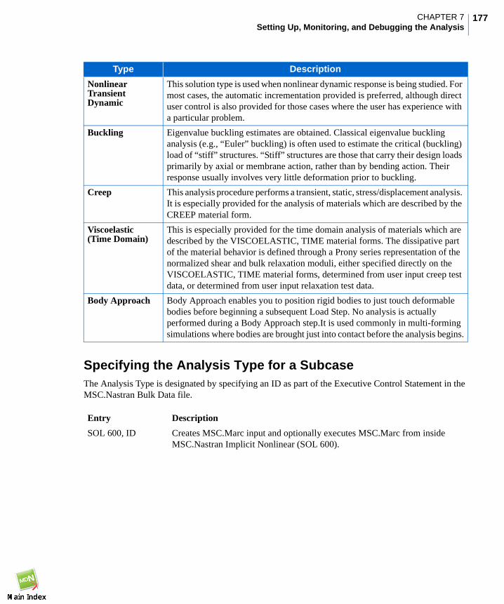
177CHAPTER 7Setting Up, Monitoring, and Debugging the Analysis
Specifying the Analysis Type for a SubcaseThe Analysis Type is designated by specifying an ID as part of the Executive Control Statement in theMSC.Nastran Bulk Data file.
NonlinearTransientDynamic
This solution type is used when nonlinear dynamic response is being studied. Formost cases, the automatic incrementation provided is preferred, although directuser control is also provided for those cases where the user has experience witha particular problem.
Buckling Eigenvalue buckling estimates are obtained. Classical eigenvalue bucklinganalysis (e.g., “Euler” buckling) is often used to estimate the critical (buckling)load of “stiff” structures. “Stiff” structures are those that carry their design loadsprimarily by axial or membrane action, rather than by bending action. Theirresponse usually involves very little deformation prior to buckling.
Creep This analysis procedure performs a transient, static, stress/displacement analysis.It is especially provided for the analysis of materials which are described by theCREEP material form.
Viscoelastic(Time Domain)
This is especially provided for the time domain analysis of materials which aredescribed by the VISCOELASTIC, TIME material forms. The dissipative partof the material behavior is defined through a Prony series representation of thenormalized shear and bulk relaxation moduli, either specified directly on theVISCOELASTIC, TIME material forms, determined from user input creep testdata, or determined from user input relaxation test data.
Body Approach Body Approach enables you to position rigid bodies to just touch deformablebodies before beginning a subsequent Load Step. No analysis is actuallyperformed during a Body Approach step.It is used commonly in multi-formingsimulations where bodies are brought just into contact before the analysis begins.
Entry Description
SOL 600, ID Creates MSC.Marc input and optionally executes MSC.Marc from insideMSC.Nastran Implicit Nonlinear (SOL 600).
Type Description

MSC.Nastran 2007 r1 Implicit Nonlinear (SOL 600) User’s Guide178
The following Solution Sequences are available with SOL 600.
References• SOL 600,ID (p. 138 in the .
Defining Analysis Type for a Subcase in MSC.Patran
To define the Analysis Type for a subcase:
1. Click on the Analysis Application button to bring up the Analysis Application form.
2. Click Solution Type... and click on the Implicit Nonlinear toggle.
3. Click Subcases... and select an analysis type from the Analysis Type pull-down menu.
References• Solution Types (p. 216 in the MD Patran MD Nastran Preference Guide, Volume 1: Structural
Analysis.
Table 7-1 Solution Sequences
SOLNumber SOL Name Description
101 SESTATIC Statics
103 SEMODES Normal Modes
105 SEBUCKL Buckling
106 NLSTATIC Nonlinear or Linear Statics
109 SEDTRAN Direct Transient Response
129 NLTRAN Nonlinear or Linear Transient Response
Other, as specified in the QRG, are available for special use.
Note: There are two ways to set up SOL 600 analysis jobs in MSC.Patran. The first is toselect Implicit Nonlinear as the Solution Type. This option gives you access to mostof the various analysis capabilities and numerical controls available throughSOL 600. The second option uses the same menus as if you were setting up a non-SOL 600 analysis, such as a SOL 106 or 129, but simply changes the executivecommand line. To use this second option, simply set up your analysis the same wayyou would a non-SOL 600 job and click on the SOL 600 Run toggle on the SolutionParameters form.

179CHAPTER 7Setting Up, Monitoring, and Debugging the Analysis
Translation ParametersTranslation parameters define file formats, numerical tolerances, processing options, numbering offsets,and include files.
Specifying the Translation ParametersThere are numerous translation parameters for SOL 600. Most of these parameters start with the lettersM, MR or MARC and follow the format MXXXX, MRXXXX, or MARCXXX.
References• Parameter Descriptions (p. 628 in the .• Format of Bulk Data Entries (p. 888 in the .• INCLUDE (p. 84 in the .
Defining Translation Parameters in MSC.Patran
To set translation parameters:
1. Click on the Analysis Application button to bring up the Analysis Application form.
2. On the Analysis Application form, click Translation Parameters...

MSC.Nastran 2007 r1 Implicit Nonlinear (SOL 600) User’s Guide180

181CHAPTER 7Setting Up, Monitoring, and Debugging the Analysis
References• Translation Parameters (p. 210 in the MD Patran MD Nastran Preference Guide, Volume 1:
Structural Analysis.
Data Output Defines the type of data output.
• XDB Buffer Size For the XDB results file, defines the buffer size used foraccessing results.
Tolerances • Division - prevents divide by zero errors.• Numerical - determines if two real values are equal.• Writing determines if a value is approximately zero when
generating a Bulk Data entry field.
Bulk Data Format • Sorted Bulk Data -• Card Format -• Grid Precision Digits - Specifies where to round off a grid point
coordinate before it’s written out to the bdf file. For example ifthis value is specified as 2 the number 1.3398 will be writtenout as 1.34.
Node Coordinates Defines which coordinate frame is used when generating thegrid coordinates.
Number of Tasks Represents the number of processors to be used to run an analysis.It is assumed that the environment is configured for distributedparallel processing.
Numbering Options... Subform used to indicate offsets for all IDS to be automaticallyassigned during translation.
Bulk Data Include File... Prompts you for the filename of the include file.

MSC.Nastran 2007 r1 Implicit Nonlinear (SOL 600) User’s Guide182
Solution ParametersSolution parameters control a range of functions in the SOL 600 analysis. Functions such asselecting the solver type, establishing a restart, specifying domain decomposition are all part of thesolution parameters.
Specifying Solution ParametersSolution Parameters are designated in the Parameters portion of the MSC.Nastran Input file with thefollowing entries.
References• Parameter Descriptions (p. 628 in the .• Format of Bulk Data Entries (p. 888 in the .• INCLUDE (p. 84 in the .
Entry Description
INCLUDE Inserts an external file into the input file. The INCLUDE statement may appearanywhere within the input data file.
NLPARM Selects the parameters used for nonlinear static analysis.
TSTEPNL Selects integration and output time steps for a nonlinear dynamic analysis.
NLSTRAT Defines strategy parameters for nonlinear structural analysis.*
NLAUTO Defines parameters for automatic load/time stepping.*
Note: *NLSTRAT and NLAUTO defaults are appropriate for most analyses and these entries arenot normally required.

183CHAPTER 7Setting Up, Monitoring, and Debugging the Analysis
Defining Solution Parameters in MSC.Patran
To set solution parameters:
1. Click on the Analysis Application button to bring up the Analysis Application form.
2. On the Analysis Application form, click Solution Type..., and select Implicit Nonlinear. Thenclick Solution Parameters...
Solver Options Specifies the solver to be used in numerically inverting the system oflinear equilibrium equations.
Contact Parameters Defines options for detecting and handling contact.
Direct Text Input This subform is used to directly enter entries in the File Management,Executive Control, Case Control, and Bulk Data sections of theMSC.Nastran input file.
Restart Parameters Includes a Restart option in the MSC.Nastran input file.
Advanced Job Control Sets alternate versions of the solver and alternate formats for theresults file.
Domain Decomposition Designates that domain decomposition be done manually,semi-automatically, or automatically.

MSC.Nastran 2007 r1 Implicit Nonlinear (SOL 600) User’s Guide184
References• For more information on Solver Options, see Numerical Methods in Solving Equations (p. 60 in
the MSC.Nastran 2005 r3 Implicit Nonlinear (SOL 600) User’s Guide.
• For more information on Contact parameters, see Contact Parameters Subform (p. 251 in theMD Patran MD Nastran Preference Guide, Volume 1: Structural Analysis.
• For more information on Restart Parameters, see Restart Parameters Subform (p. 256 in the MDPatran MD Nastran Preference Guide, Volume 1: Structural Analysis.
• For more information on Domain Decomposition, see Domain Decomposition (p. 258 in the MDPatran MD Nastran Preference Guide, Volume 1: Structural Analysis.

185CHAPTER 7Setting Up, Monitoring, and Debugging the Analysis
SubcasesCreating multiple subcases allows you to efficiently analyze multiple load cases in one run. Each subcaseis a collection of loads and boundary conditions, output requests, and other parameters. For nonlinearanalysis runs the starting point of each subcase is the ending point of the previous subcase.
Specifying SubcasesEach subcase is designated with the following Case Control Command.
References• SUBCASE (p. 463 in the .
Defining Subcases in MSC.Patran
To define a subcase:
1. Click on the Analysis Application button to bring up the Analysis Application form.
Entry Description
SUBCASE Delimits and identifies a subcase.

MSC.Nastran 2007 r1 Implicit Nonlinear (SOL 600) User’s Guide186
2. From the Analysis Application form click Subcases...

187CHAPTER 7Setting Up, Monitoring, and Debugging the Analysis
Subcase Name Specifies a name for a new subcase.
Available Load Cases Selects one or more available load cases to be applied to thenew subcase.
Subcase Options
• Subcase Parameters Controls load increment and iteration parameters for the subcase. Alsodefines the nonlinear effects for the subcase. See SubcaseParameters, page 188.
• Output Requests Defines the nodal and element results quantities and also determinesthe frequency of results reporting. See Output Requests (Ch. 8).
• Direct Text Input This subform is used to directly enter entries in the File Management,Executive Control, Case Control, and Bulk Data sections of theMSC.Nastran input file.
• Select Superelements Defines which superelements are to be included in the subcase.
• Select Explicit MPCs Selects explicit MPCs to be included in the subcase.

MSC.Nastran 2007 r1 Implicit Nonlinear (SOL 600) User’s Guide188
Subcase ParametersThe subcase parameters represent the settings in MSC.Nastran Case Control and Bulk Data Section thattake effect within a subcase and do not affect the analysis in other subcases. Subcase parameters aredependent on the type of analysis being performed. The set of subcase parameters applicable for eachanalysis type are described in the following sections. For more information, see Solution Methods andStrategies in Nonlinear Analysis (Ch. 3) in the MSC.Nastran 2005 r3 Implicit Nonlinear (SOL 600)User’s Guide.
Specifying Static Subcase ParametersFor static nonlinear analysis the subcase parameters control the iteration process and theload incrementation.
References• NLPARM (p. 377 in the .• NLPCI (p. 1999 in the .• NLAUTO (SOLs 400/600) (p. 1983 in the .• NLSTRAT (SOL 600) (p. 2005 in the .
Defining Static Subcase Parameters in MSC.Patran1. Click the Analysis Application button to bring up Analysis Application form. Click on Solution
Type and check to see that Implicit Nonlinear is the selected Solution Type, then click OK.
2. On the Analysis form select Subcases... and choose Static from the Analysis Typepull-down menu.
Entry Description
NLPARM Nonlinear Static Analysis Parameter Selection.
NLPCI Defines a set of parameters for the arc-length incremental solution strategies innonlinear static analysis.
NLAUTO Defines parameters for automatic load/time stepping used in SOL 600.
NLSTRAT Defines strategy parameters for nonlinear structural analysis used in SOL 600.

189CHAPTER 7Setting Up, Monitoring, and Debugging the Analysis
3. Click Subcase Parameters...
Linearity Prescribes the nonlinear effects for the subcase.
Nonlinear Solution Parameters
• Nonlinear Geometric Effects Defines the type of geometric or material nonlinearity to beincluded in the subcase.
• Follower Forces Specifies whether forces will follow displacements.
Load Increment Params... Defines whether the load increments will be fixed or adapted ineach iteration and the method by which adaptive loadincrements will be determined.
Iteration Parameters... Sets forth the iterative procedures that are employed to solve theequilibrium problem at each load increment.
Contact Table... Activates, deactivates, and controls the behavior of contactbodies in the analysis.
Active/Deactive Elements... Defines groups of elements to be active or deactive forthe subcase.

MSC.Nastran 2007 r1 Implicit Nonlinear (SOL 600) User’s Guide190
Specifying Normal Modes Subcase ParametersFor normal modes nonlinear analysis the subcase parameters control the eigenvalue extractiontechniques and the range of frequencies to be targeted for extraction.
References• EIGR (p. 1462 in the .• EIGRL (p. 1466 in the .
Defining Normal Modes Subcase Parameters in MSC.Patran1. Click the Analysis Application button to bring up Analysis Application form. Click on Solution
Type and check to see that Implicit Nonlinear is the selected Solution Type, then click OK.
2. On the Analysis form select Subcases... and choose Normal Modes from the Analysis Typepull-down menu.
Entry Description
EIGR Defines data needed to perform real eigenvalue analysis.
EIGRL Defines data needed to perform real eigenvalue (vibration or buckling) analysiswith the Lanczos method.

191CHAPTER 7Setting Up, Monitoring, and Debugging the Analysis
3. Click Subcase Parameters...
Extraction Method Defines the method to use to extract the real eigenvalues.
Lancozs Parameters
• Number of Modes Indicates an estimate of the number of eigenvalues to be located.
• Lowest/Highest Frequency Defines the lower and upper limits to the range of frequencies tobe examined.
Sequence Checking Requests that Sturm sequence checking be performed on theextracted eigenvalues.

MSC.Nastran 2007 r1 Implicit Nonlinear (SOL 600) User’s Guide192
Specifying Buckling Subcase ParametersFor nonlinear buckling analysis the subcase parameters control the eigenvalue extraction techniques andthe range of frequencies to be targeted for extraction.
A METHOD command is specified in the desired subcase and selects an EIGB, or EIGRL BulkData entry.
The linear buckling load analysis is correct when you take a very small load step in increment zero, ormake sure the solution has converged before buckling load analysis (if multiple increments are taken).
In a buckling problem that involves material nonlinearity (for example, plasticity), the nonlinear problemmust be solved incrementally. During the analysis, a failure to converge in the iteration process ornonpositive definite stiffness signals the plastic collapse.
For extremely nonlinear problems, the EIGB option cannot produce accurate results. In that case, useNLSTRAT options to specify an arc-length method that allows automatic load stepping in a quasi-staticfashion for both geometric large displacement and material (elastic-plastic) nonlinear problems. Theoption can handle elastic-plastic snap-through phenomena. Therefore, the post-buckling behavior ofstructures can be analyzed.
The eig option must be specified with the OUTR option on SOL 600 Executive Control statement if op2,xdb, pch, or .f06 options are specified and MSC.Marc performs natural frequency or buckling eigenvalueanalysis. The reason it must be provided on the SOL entry is to enable MSC.Nastran to create DMAP onthe fly which include the LAMA data block. If the eig option is omitted, eigenvectors will be present inthe MSC.Nastran output but no eigenvalues will be available.
References• eig (p. 142 in the .• METHOD (p. 353 in the .• EIGB (p. 1454 in the .• EIGRL (p. 1466 in the .• MARCRBAL (p. 705 in the .
Entry Description
METHOD Selects the real eigenvalue extraction parameters.
EIGB Defines data needed to perform buckling analysis.
EIGRL Defines data needed to perform real eigenvalue (vibration or buckling) analysiswith the Lanczos method.
MARCRBAL This parameter is used for eigenvalue analysis where natural frequencies orbuckling modes need to be calculated using the deformed geometry from anonlinear analysis.

193CHAPTER 7Setting Up, Monitoring, and Debugging the Analysis
Defining Buckling Subcase Parameters in MSC.Patran1. Click the Analysis Application button to bring up Analysis Application form. Click on Solution
Type and check to see that Implicit Nonlinear is the selected Solution Type, then click OK.
2. On the Analysis form select Subcases... and choose Buckling from the Analysis Typepull-down menu.
3. Click Subcase Parameters...
Specifying Transient Dynamic Subcase ParametersFor transient dynamic nonlinear analysis the subcase parameters control the iteration process and theload incrementation.
References• TSTEPNL (p. 489 in the .• NLAUTO (SOLs 400/600) (p. 1983 in the .• NLSTRAT (SOL 600) (p. 2005 in the .
Extraction Method Defines the method to use to extract the real eigenvalues.
Lancozs Parameters
• Max # of Modes Indicates the maximum number of eigenvalues to be located.
• Max # of Modesw/Pos. Eigenvalues
Indicates the maximum number of positive eigenvalues to be located.
Entry Description
TSTEPNL Nonlinear Dynamic Analysis Parameter Selection.
NLAUTO Parameters for automatic load/time stepping.
NLSTRAT Strategy Parameters for nonlinear structural analysis.

MSC.Nastran 2007 r1 Implicit Nonlinear (SOL 600) User’s Guide194
Defining Transient Dynamic Subcase Parameters in MSC.Patran1. Click the Analysis Application button to bring up Analysis Application form. Click on Solution
Type and check to see that Implicit Nonlinear is the selected Solution Type, then click OK.
2. On the Analysis form select Subcases... and choose Transient Dynamic from the Analysis Typepull-down menu.
3. Click Subcase Parameters...
Linearity Prescribes the nonlinear effects for the subcase.
Nonlinear Solution Parameters
• Nonlinear Geometric Effects Defines the type of geometric or material nonlinearity to beincluded in the subcase.
• Follower Forces Specifies whether forces will follow displacements.
Load Increment Params... Defines whether the load increments will be fixed or adapted ineach iteration and the method by which adaptive loadincrements will be determined.

195CHAPTER 7Setting Up, Monitoring, and Debugging the Analysis
Specifying Creep Subcase ParametersThe creep analysis option is activated in MSC.Nastran through the CREEP Bulk Data entry. The creeptime period and control tolerance information are input through the MARCAUTO=1 parameter. Thisoption can be used repeatedly to define a new creep time period and new tolerances. These tolerancesare defined in the section on Creep Control Tolerances. Alternatively, a fixed time step can also bespecified through the MARCAUTO parameter. In this case, no additional tolerances are checked forcontrolling the time step.
Creep analysis is often carried out in several runs using the RESTART Bulk Data entry. Save restart filesfor continued analysis. The RESTART entry allows you to reset the parameters defined in MARCAUTOupon restart.
References• MATVP (SOL 600) (p. 1613 in the MSC.Nastran Quick Reference Guide.• NLPARM (p. 1991 in the .• MARCAUTO (p. 686 in the .• RESTART (SOLs 600/700) (p. 2330 in the MSC.Nastran Quick Reference Guide.
Defining Creep Subcase Parameters in MSC.Patran1. Click the Analysis Application button to bring up Analysis Application form. Click on Solution
Type and check to see that Implicit Nonlinear is the selected Solution Type, then click OK.
2. On the Analysis form select Subcases... and choose Creep from the Analysis Typepull-down menu.
Iteration Parameters... Sets forth the iterative procedures that are employed to solvethe equilibrium problem at each load increment.
Contact Table... Activates, deactivates, and controls the behavior of contactbodies in the analysis.
Active/Deactive Elements... Defines groups of elements to be active or deactive for thesubcase. Note that this option uses the equivalent of direct textinput (MARCIN option) and is not explicitly supported bySOL 600.
Entry Description
NLPARM Nonlinear Static Analysis Parameter Selection.
MATVP Defines creep characteristics based on experimental data or known empiricalcreep law.
MARCAUTO Determines which MSC.Marc’s increment option is used.
RESTART Specifies writing or reading of restart data for Nonlinear Analysis whenMSC.Marc is executed from MSC.Nastran.

MSC.Nastran 2007 r1 Implicit Nonlinear (SOL 600) User’s Guide196
3. Click Subcase Parameters...:

197CHAPTER 7Setting Up, Monitoring, and Debugging the Analysis
Specifying Body Approach Subcase ParametersFor body approach analysis the subcase parameters control the iteration process and theload incrementation.
References• “BCMOVE” in the MSC.Nastran Quick Reference Guide.
Defining Body Approach Subcase Parameters in MSC.Patran1. Click the Analysis Application button to bring up Analysis Application form. Click on Solution
Type and check to see that Implicit Nonlinear is the selected Solution Type, then click OK.
2. On the Analysis form select Subcases... and choose Body Approach from the Analysis Typepull-down menu.
Creep Solution Parameters
• Procedure Selects Implicit or Explicit Creep method.
• Nonlinear Geometric Effects Defines the type of geometric or material nonlinearity to beincluded in the subcase.
• Follower Forces Specifies whether forces will follow displacements.
Increment Type Defines a fixed or adaptive increment method.
• Adaptive IncrementParameters...
For adaptive methods, sets boundaries for incrementation.
Iteration Parameters Sets forth the iterative procedures that are employed to solvethe equilibrium problem at each load increment.
Contact Table... Activates, deactivates, and controls the behavior of contactbodies in the analysis.
Active/Deactive Elements... Defines groups of elements to be active or deactive forthe subcase.
Entry Description
BCMOVE Specifies movement of rigid surfaces.

MSC.Nastran 2007 r1 Implicit Nonlinear (SOL 600) User’s Guide198
3. Click Subcase Parameters...
Body Approach Parameters
• Total Time Places a time step option in the Load Step.
• Synchronized If ON, specifies that when the first rigid body comes into contact, therest stop moving.
Contact Table... Activates, deactivates, and controls the behavior of contact bodies inthe analysis.

199CHAPTER 7Setting Up, Monitoring, and Debugging the Analysis
Execution Procedure for MSC.Nastran ImplicitNonlinear from the Command LineAfter the generation of the input file is complete, it is submitted for execution as a batch process(MSC.Nastran is not an interactive program). Once the input file has been submitted, you have noadditional interaction with MSC.Nastran until the job is complete except that you can terminate the jobprior to completion if it becomes necessary and monitor several keys files such as, .f04, .sts, .log, etc.
MSC.Nastran is executed with a command called nastran. (Your system manager may assign a differentname to the command.) The nastran command permits the specification of keywords used to requestoptions affecting MSC.Nastran job execution. The format of the nastran command is:
nastran input_data_file [keyword1 = value1 keyword2 = value2 ...]
where input_data_file is the name of the file containing the input data and keywordi=valuei is one ormore optional keyword assignment arguments. For example, to run an a job using the data fileexample1.dat, enter the following command:
nastran example1
See The nastran Command (p. 2 in the .
The details of submitting an MSC.Nastran job are specific to your computer system— contactyour computer system personnel or your MSC.Nastran Installation and Operations Guide forfurther information.

MSC.Nastran 2007 r1 Implicit Nonlinear (SOL 600) User’s Guide200
Using MSC.Patran to Execute MSC.NastranThe Analysis Application controls the execution of MSC.Nastran.
When the Action is set to Analyze, the Method is set to Full Run, and the Apply button is selected fromthe Analysis form, a jobname.bdf file is created which contains the analysis model, and theP3TRANS.INI script is spawned by MSC.Patran. This script controls the analysis process outside andindependent of MSC.Patran.
When the analysis is successfully completed, one or more output file is produced. These output files canbe directly imported or attached into the MSC.Patran database for postprocessing by setting the Actionmenu to Access Results.
How to Tell When the Analysis is DoneIf you submit the job from the MSC.Nastran icon (i.e., outside MSC.Patran), as long as the parentwindow the job was run from is active, the analysis is still running. If you submit the job from withinMSC.Patran and use -stdout when you execute MSC.Patran, you can look in the MSC.Patran parentwindow and it will tell you when it submits the Nastran job, and also when the Nastran job is completed.Of course you can always use the Analysis Manager. Once the job is complete look in the parent windowto see what files were generated.

201CHAPTER 7Setting Up, Monitoring, and Debugging the Analysis
How to Tell if the Analysis Ran SuccessfullyLook in the working directory and you will see the typical jobname.f06, jobname.f04,jobname.log. If these files are there, you successfully submitted the Nastran job. If you submitted ajob with SOL 600, xxx as the executive command, there will also be some jobname.marc.xxx filesin the subdirectory. These are the files from the Marc run. To see if the run was successful, openjobname.marc.sts and look for the number at the bottom. For most analyses, 3004 means the runwas successful.
For others, such as thermal contact, generation of DMIG matrices for subsequent use, other exit codessuch as 3031, 3030, 3031, and 3022 mean a successful run. Exit code 13 signifies a dta input error whichmust normally be evaluated by MSC development. Exit 3015 means the job diverged and requiresadditional time steps, changes to convergence controls or other changes to the input. A brief descriptionof most errors is provided at the end of this jid.mar.out file.
If there are no jobname.marc.xxx files, check to make sure you can submit Marc jobs successfully.At the end of the jobname.f06 file, Nastran will tell you what command it used to submit the Marcjob. Take this command to a command prompt and enter it to see why the Marc job wasn’t submitted. Ifyou can go to a command window and type in “run_marc jid-jobname“ and it finds the Marcexecutable and runs the jobname.dat Marc input file, you can just use PATH=2 on the SOL 600command line.

MSC.Nastran 2007 r1 Implicit Nonlinear (SOL 600) User’s Guide202
Monitoring the AnalysisThe nastran command permits the specification of keywords used to request options affectingMSC.Nastran job execution. The format of the nastran command is:
nastran input_data_file [keyword1 = value1 keyword2 = value2 ...]
where input_data_file is the name of the file containing the input data and keywordi=valuei is one or moreoptional keyword assignment arguments.
Use the keyword xmonast to monitor a MSC.Nastran job as described below.
For more information, see The nastran Command (p. 2 in the .
MSC.Nastran Implicit Nonlinear provides a status file (jobname.marc.sts) that can be queriedperiodically to see how the analysis is progressing and if the job is completed. The file will report theinformation relating to the progress of the analysis, with warning and informative messages.
The file review is especially important when manual or automatic time stepping procedures are beingused to step through an analysis procedure. One line is written after each successful increment. Anexample file output is shown below.
Figure 7-1 information Summary of Job: nas.cant_bmsm.marc
The first column shows the procedural step, while the second column shows the increment number. Notethat not every increment size is equal, as can be seen in the “TimeStep of the INC” column. For thisexample, the third increment size is larger than the first two increments, which means that the procedureis satisfied that equilibrium is being satisfied and that it has increased the time step size to take advantage
xmonast xmonast={yes|no|kill Default: No
Indicates if XMONAST is to be run to monitor the MSC.Nastran job. If “xmonast=yes” isspecified, XMONAST will be automatically started; you must manually exit XMONASTwhen the MSC.Nastran job has completed. If “xmonast=kill” is specified, XMONAST willstart and will automatically exit when the MSC.Nastran job has completed.
Example: nastran example xmon=kill
This example runs the XMONITOR utility while the MSC.Nastran job is running. Oncethe job completes, the XMONITOR program is automatically terminated.
dip

203CHAPTER 7Setting Up, Monitoring, and Debugging the Analysis
of the better convergence characteristics. The third column (“cycle# of the Inc) indicates the number ofNewton Raphson iterations made during this increment. The next three columns show the incrementinformation, while the next six columns show the numbers for the total analysis.
Sepa means number of contact separations, cut refers to the number of time step size cutbacks, and splitrefers to the number of increment splits due to contact penetration.
If the increment size becomes small, and there are a number of increments of this size, the analysis hasprobably “stalled”, indicating that convergence is becoming very difficult to attain for the problem. Areview of the model is indicated.
The max disp column provides a valuable means to tell if a job is diverging or in some other way notproceeding correctly.
Editing a MSC.Nastran Input FileThere may be instances when you want to directly edit the MSC.Nastran Bulk Data file. Someexperienced MSC.Nastran users may want to add options directly to specific Parameters and Bulk Dataentries. MSC.Patran provides direct access to the Bulk Data file as follows.
To edit an existing Bulk Data File:
1. Click on the Analysis Application icon to bring up the Analysis Application form.
2. Set the Action>Object>Method combination to Analyze>Existing Deck>Full Run.
3. Click Edit Input File...
MSC.Patran automatically looks for an existing deck name that matches the current databasename and displays the existing deck.

MSC.Nastran 2007 r1 Implicit Nonlinear (SOL 600) User’s Guide204
Debugging the AnalysisMSC.Nastran generates a substantial amount of information concerning the problem being executed. The.f04 file provides information on the sequence of modules being executed and the time required by eachof the modules; the .log file contains system messages.
MSC.Nastran may terminate as a result of errors detected by the operating system or by the program. Ifthe DIAG 44 is set (see the diag keyword (p. 253) and the MSC.Nastran Quick Reference Guide),MSC.Nastran will produce a dump of several key internal tables when most of these errors occur.Before the dump occurs, there may be a fatal message written to the .f06 file. The general format ofthis message is
***SYSTEM FATAL ERROR 4276, subroutine-name ERROR CODE n
These messages are SEVERE WARNING, or other text ... issued whenever an interrupt occurs thatMSC.Nastran is unable to satisfactorily process. The specific reasons for the interrupt are usually printedin the .f06 and/or .log file.
Resolving Convergence ProblemsThere are three major steps in getting a complete solution.
1. get the model input debugged (see section titled “Exit 13 Errors”).2. establish initial equilibrium (see section titled “Exit 2004 Errors”).3. getting the analysis to run to completion.
Step 1: De-Bugging the Model Input
See How to Tell if the Analysis Ran Successfully, page 201.
To Debug a Failed Analysis
First, check the .sts, .f04, .f06, or .out files for licensing, disk access or format errors. The number a thebottom of the jobname.marc.sts is the Marc Exit Number. Exit 13 means there was a format error in theMarc input. Exit 2004 generally means you have unconstrained degrees of freedom or rigid body modes.3002 means the analysis got part way through and then stopped. The complete Marc Exit message isgiven at the end of the jobname.marc.out file, which may also be in jobname.f06 depending on the valueof COPYR.
If you get an Exit 13 check your input, make sure everything you need is in the Nastran input deck. Checkfor elements, grids, contact body creation, etc. An easy way to debug these type of problems is to readthe jobname.marc.dat file (the Marc input file Nastran created) in to Mentat or Patran (an empty db withpreference set to Marc) and see what is missing. Often you will see that some elements are missing, orthat the contact bodies were not created as you would expect them. For more information see Figure 7-2.

205CHAPTER 7Setting Up, Monitoring, and Debugging the Analysis
Figure 7-2 Flowchart to Debugging a SOL 600 Run
Submit job
Wait until processfinishes.
Does .stsfile exist?
Do.f06, .f04,.log filesexist?
Isthere a Fatal
Error Messagein .f06, .f04,
.log?
Ck Marc submit card,find in .f06 and typein a cmd window tosee why Marc job
was not submitted.
no yes no
Nastran job submitfrom windows
w/Pause=YES, ckerror msg
no
ck .sts forExit #
fix-it - typicalNastran debug
IsExit
#=3004?
yesyes
Do youget Nastranrequested
formatted output,such
as .xdb?
yes Successful completion- go on to postprocess
yes
look injobname.marc.out forExit # and message.
ck T160P2.exe run, on windowsmake sure it is in search path.
IsExit #=13?
Follow instructions in exit msg; ifits a formatting error ck Marc,Volc, or read thejobname.marc.dat file intoPatran’s Marc pref (or Mentat)and compare this modelw/original. The problem may bedisplayed when the file is read in.
IsExit #=3002?
IsExit #=2004?
Some convergenceincrements exist,postprocess them & lookfor possible causes ofstability loss, such ascontact changes. Ck
, you may beencountering bucklingmodes. Do a bucklingsolution to see or try anarc-length method.
δmax
No convergedincrements, likelyunconstrained rigidbody motion exists: a.)do modal to ID them,b.) Ck equivalencing ofmodal integrity, c.) addconstraints or weaksprings, d.) see sectionon convergenceproblems.
no
no
yes
no no
yes
yes

MSC.Nastran 2007 r1 Implicit Nonlinear (SOL 600) User’s Guide206
Step 2: Establishing Initial Equilibrium
If you get an Exit 2004 it means that the model was unable to reach equilibrium for the loads andconstraints applied in the initial subcase. Options include:
• adding more constraints (or equivalently soft springs) to ground the model.• run a modal analysis to identify unconstrained rigid body modes.
Step 3: Getting the Analysis to Run to Completion
The first thing to check at this point is: “Has the solution gone as far as it can,” i.e. maybe you alreadyhave the complete solution. Sometimes nonlinear loading causes structures to buckle which may takeyour analysis into the post-buckled region. Depending on the type of buckling, you may be simply tryingto drive your analysis farther into the post-buckling range which may not give you the information youare after. For example, if you load a frame structure with a load that exceeds the critical buckling loadand the analysis is simply working to drive the structure further into a plastic hinge.
Things to Do to Fix Non-Convergence• Check the .sts, .log, and .out files for Exit 2004, 3002, or 3003 format error messages.
• If using fixed load incrementation try using a smaller time step, or use the automatic cutbackfeature, or use adaptive time-stepping.
• Try running an eigenvalue buckling solution to see if you’ve passed a critical buckling load orexamine the stresses and strains to see if some portion of the structure has failed (if MATFfailure criteria was not included in the modal).
• If using Contact set the Contact Tolerance Bias to 0.9, particularly if doing shell contact (done bydefault in SOL 600).
• Turn on Quasi-Static inertial damping or Non-Positive Definite to eliminate un-constrained rigidbody motions (done by default in SOL 600).
• Try running an eignevalue modal solution to identify unconstrained rigid body modes.
• Try using an arc-length method - you may be encountering local buckling.
• Look at any available results of converged increments.
• If doing contact try a different contact tolerance value.
• Isolate Non-linearities and add them one at a time.
• Making Sure Appropriate Non-linearities are Included.
• Check Material Stability – Make sure the entire strain range is covered by the material data.
For complex models involving multiple forms of nonlinear behavior the “tried and true” approach(particularly if you are new to this type of problem) is to start with a linear model and add non-linearitiesone at a time. Alternatively, remove the non-linearities one at a time until it runs. This approach helpsyou determine which type of non-linearity is causing the convergence problem. If you have contact,remove it and let the bodies “pass through” one another or replace the contact condition with anequivalent displacement constraint. If you have nonlinear materials replace them with simple elastic

207CHAPTER 7Setting Up, Monitoring, and Debugging the Analysis
ones. Add the non-linearities back one at a time, making sure the behavior is reasonable and correct.Look at reaction forces and displacements of any converged increments to make sure they are of theexpected magnitude.
If you run the analysis and it doesn’t run at all, or ends before completing, you will get an error messagein the .OUT or .LOG file that will give you an indication of what the problem is. Do a text search on theword “error” in the .OUT file. The first thing to check is to make sure you were able to get a license torun the job. Licensing problems are one of the most common reasons for a run to fail. If you are sure youhave a license and submit the job correctly you should get a .OUT file that will end with an Exit #preceded by a description of why the run stopped. Common Exit #’s are: Exit 3004 – means success, i.e.the job ran to completion and did everything you asked it to. Exit 13 – means you have a syntax error inthe input file. You should check the input syntax of the line the error message points to, but it is likelythat the actual error was in the input block PRIOR to where the message points. Exit 2004 – typicallymeans non-convergence due to rigid body motions. See recommendations for Equilibrium. Exit 3002 –this means the analysis ran into convergence problems part way through and did not complete. Any ExitMessage of 3000 or higher means there are converged increments. Plot the converged increments to seewhat is going on. See Technical Application Note 4575 or Appendix A of Volume C: Program Input fora more complete list with suggested “fixes.”
Things to consider if your model doesn’t converge:1. Equilibrium - Make sure your model has LBC’s and contact conditions that will ensure force
equilibrium at EVERY increment/iteration and for ALL rigid-body modes (typically there are 6).When in doubt eliminate this as the source of non-convergence by intentionally over-constrainingthe model (or adding soft springs) and then removing constraints one at a time until you figureout the unconstrained rigid body mode. One area that is sometimes overlooked regardingequilibrium is that of the rigid body control. If you don’t specify adequate control information(e.g. you forget to add the zero that fixes the rigid body rotation value) you may haveconvergence problems.
2. LBC’s - When LBC’s are removed, the forces/pressures (and the reaction forces due todisplacement constraints) are removed gradually over the subsequent step. The forces andpressures are always removed gradually, but the reaction forces of displacement constraints maybe are removed suddenly at the beginning of the subsequent step. This sudden change in loadingcan cause convergence problems.
3. Stability and Collapse - Non-convergence will occur when a structural instability (i.e., buckling)mode is encountered. Buckling can occur either locally (in highly stressed area where the stabilityof individual elements is exceeded) or globally when the critical buckling load of any part of themodel is exceeded. You may want to do a linear buckling analysis to determine the load thatwould buckle the least-stable part of the structure. If you suspect that you are approaching thepost-buckled region here are some other things to try: a) try using Quasi-static inertial damping(turn this on under Analysis – Step Create – Solution Parameters) or one of the Arc-lengthmethods. This will help get through the unstable region if doing a snap-through bucklingproblem, and may help get you past one or two elements of local buckling, but probably not morethan that.) try a finer mesh (smaller elements have shorter length and so higher Pcr);

MSC.Nastran 2007 r1 Implicit Nonlinear (SOL 600) User’s Guide208
4. Materials - Make sure that the material coefficient values are realistic and that the models willsupport the stresses and loads developed in the model. For example if you hang a 1000 lb. weightfrom a perfectly plastic wire with a 0.001 in**2 cross section and a 20 ksi yield stress, theresulting 100 ksi stress cannot be supported by the (20 ksi yield stress) material and the run willnot converge. Comparable behavior in bending is referred to as a “plastic hinge.” Units mis-matches will often result in this type of problem (note that this only occurs in non-linear analyses).For example, let’s say you are modeling a cantilever beam and using a perfectly plastic materialmodel and a “follower force” tip load, and you mistakenly add an extra zero to the tip load. Aplastic hinge will develop with the beam “winding up” like a spring and the analysis continuingto run until it runs out of increments (which may take a long time). If you suspect this type ofproblem first run the problem with a small fraction of the load to see if it will converge. If you areusing an orthotropic or hyperelastic material it is possible to select combinations of materialproperties that will result in a non-positive definite material coefficient matrix. Normally theanalysis code will warn you if you violate this requirement.
5. Contact - If there is a problem with “chattering” (a condition where a particular node jumps intoand out of contact thus preventing the increment from converging), you can go to TranslationParameters – Contact Control Parameters – Separation and set the Chattering toggle to“Suppress”. The parameters which have the biggest effect on contact behavior are “ContactDistance Tolerance”, D (see Fig. 1), “Bias Factor,” B (see Fig. 2) -) and “Separation Force.” Thedefault uses D = 1/20 the of the element edge length. You can find the specific value in the.OUTfile and try a larger or smaller value, whichever you feel is most appropriate. The default on thebias value is 0, if having problems with contact one of the first things to try is to over-ride thisvalue on the Analysis – Translation Parameters – Contact Detection – Contact Parameters formwith 0.9. Another option would be to increase the separation force (which defaults to 0) to preventchattering. When considering contact problems look for places (such as corners and otherdiscontinuities) where one contact surface may “slip” off.
Standard Steps to Resolving Convergence Problems:
If your model doesn’t run, or stops pre-maturely: FIRST, READ THE MESSAGES IN The .sts, .f06, .logand .out files. Common causes of the run to fail include:
1. unconstrained rigid body modes.2. you're in the post-buckled region.3. problems resolving contact.4. some part of the model/material is "over-constrained" such that the given displacement solution
doesn’t change when the load is increased (i.e. individual elements are buckling locally), this typeof non-unique solution can prevent convergence.
After trying the obvious things, talk to other experienced users about possible reasons your run isn’tworking. In one case, a user was using the standard element formulation with = 0.5 and hex/21elements and his model would not converge even though there were no obvious problems. For this case,using the constant volume formulation should provide a unique solution and allow convergence, unless
= 0.5 causes numerical problems. In that case you should use the Herrmann elements which shouldtake care of the numerical problems as well as the non-unique solution problem. If these options don’twork, you could try using reduced integration, which may solve both problems at once, but may
υ
υ

209CHAPTER 7Setting Up, Monitoring, and Debugging the Analysis
have problems with energy-free or "spurious" deformation modes (also called "hour-glassing"),although the analysis has built-in hour glass stabilization. Also, try quasi-static inertial damping or anarc-length methods.
Here are some other things to try:
a. try a finer mesh;
b. modify the material model: if its simple elastic-perfectly plastic with large plastic strains tryusing constant volume Herrmann elements, if using a hyper-elastic material model trylowering Nu from 0.5 to maybe 0.49 or so (or lower if you have to); make sure its based ontest data that includes the type of behavior you are trying to model (i.e. if your test data is froma uni-axial tensile test and you are modeling a pressurized cylinder, which is a bi-axial stressstate, try analyzing a simple bi-axial sheet to see if your hyper-elastic material model willsuccessfully handle bi-axial stress states; if not you may have to include some bi-axial testdata (hyper-elastic models based on test data should include at least 2 "modes," although theprogram has a new Arruda-Boyce model which often yields better results with limitedexperimental data);
c. simplify - if the model you are running is a 3D cylinder made of solid elements, run a 2D axi-symmetric test case to check out the mesh refinement and material model. If not in the post-buckled region try: 1) look at deformed shape to see if it looks reasonable. Remember thatstatic equilibrium must be maintained at every step; 2) check reaction forces to see if the loadpath is reasonable; 3) look for highly distorted elements, both visually and in the .out file - ifyou find any you may need to go back and refine your mesh in that area to keep those elementswell-behaved, i.e. converging, or use adaptive re-meshing. Although distorted elements willnormally just give you bad results but not necessarily prevent convergence. Typically linearelements (i.e. quad/4 instead of quad/8) do better in analyses where severe distortion isexpected. 4) if using contact elements you may be able to ease convergence problems bysimplifying the contact interaction: a) look at the .sts file for the # of increment splits and # ofseparations to see if contact is the problem; b) set bias to 0.9, increase (or decrease) the contacttolerance distance, suppress chattering; c) modify the contact table to eliminate suspectedtrouble areas (at least as a diagnostic measure); d) look for areas where contact bodies may be“sliding off. 5) PAY ATTENTION TO THE MESSAGES IN THE .STS, .LOG, .f06 AND.OUT FILES, they may tell you why the model was not translated or convergence was notreached and the analysis terminated. 6) if non-convergence relates to inelastic behavior of thematerial, such as in a plasticity analysis, make sure there are no "plastic hinges" formed,where static equilibrium cannot be achieved because the material is not strong enough, in thiscase all the iterations go to deforming the body around the plastic region and staticequilibrium may never be reached. 7) when doing a hyperelastic material analysis the materialmodel may be unpredictable since the coefficients are generally quite unintuitive. The runmay not converge simply because the material model, while it may look reasonable, mayactually be inherently unstable (things like negative energy behavior, etc.) 8) make sure youaren't stuck at a stability bifurcation point, (i.e. at a buckling mode), what may be happeningis that there are 2 valid (post-buckling in this case) equilibrium paths and the code flips backand forth between them preventing convergence; the way to get past this is to make theproblem dynamic and use the inertia of the body to "select" the appropriate equilibrium path.

MSC.Nastran 2007 r1 Implicit Nonlinear (SOL 600) User’s Guide210
Again, the “tried and true” method is to start with a linear model and add non-linearities one at a time, orremove nonlinearities.
Consider changing the Contact Distance Tolerance. If you run into contact-related convergence problemsthis is one of the first things to try.
Standard Exit MessagesPlease refer to the MSC.Nastran Quick Reference Guide and the MSC.Nastran Reference Manual for exitcodes and numbers.
SOL 600 Exit Numbers and their Interpretation:
Most SOL 600 jid.marc.out files end with an EXIT MESSAGE & NUMBER. This exit number is locatedin the last few lines of the output file (.out file) of the SOL 600 run. If a.out file is not created, thatsometimes points to an installation issue or a FATAL ERROR or SEVERE WARNING will be present inthe jid.f06 file. EXIT #3004 is GOOD. It indicates a successful run. Most other exit numbers indicate afailed run. Below are some common exit numbers that a user might encounter. Information on more exitnumbers are given in Volume C (Program Messages) of SOL 600 documentation, which contains the fulllist of exit numbers/messages.
1. Exit 13: This exit # indicates an error with the SOL 600 input file. SOL 600 gives an exit 13if it does not understand some term in the input deck. Causes include either the input deck iswritten out incorrectly, or because the set-up is inconsistent (user set-up issue) e.g. user may setup a shell model and not provide shell thickness; or the user creates but neglects to assignmaterial properties.
Fixing ‘exit 13’ errors: Go to the.out file and search for the keyword: error (*** error). The errormessage listed there points to the section/line of the input deck causing the problem. The user hasto figure out why that is incorrect, along the lines discussed in the above paragraph or send theMSC.Nastran implicit file (2) to MSC.
2. Exit 2004: If the user gets this message as soon as the job is submitted - i.e. noincrements/iterations successfully completed, it points to an unconstrained mesh. Exit 2004, froma numerical stand-point, indicates a non-positive definite stiffness matrix. From a model set-upstand-point, this implies that the mesh is not constrained in space, i.e. either incomplete (or no)BCs have been applied to the model. User needs to check the BCs.
If this exit number comes after the analysis begins i.e. after some increments are done, the reasonsare to do with the mechanics of the model e.g. formation of a plastic hinge, or due to buckling, ora deformable body sliding due to lack of friction in the model. The fix for each situation is uniqueto the underlying physics of the model e.g. adding friction if that reflects the actual situation.Turning on the “Suppress Rigid Body Motion” option on the NonLinear Solution parameters canhelp in some cases.

211CHAPTER 7Setting Up, Monitoring, and Debugging the Analysis
3. Exit 1005, Exit 1009: If this exit message (exit 1005) comes as soon as the job is submitted i.e.at the first assembly of the first iteration, it indicates a meshing problem. Re-check mesh and re-mesh. In most cases, this error message(s) comes after an analysis has started. Both exit numbers1005 & 1009 indicate excessive element deformation during a particular load increment, in aparticular iteration. The way to get around this error is to reduce step size. However SOL 600 doesthat automatically and if the problem still persists it gives exit 3015/3009. See explanationsbelow on exit 3015/3009.
4. Exit 3002: This message indicates that SOL 600 has reached the user-specified upper limit onthe number of (Newton-Raphson) iterations within a load increment. The default is set to 25.SOL 600 keeps iterating 25 times, and tries to converge to a solution for that increment. If thatdoes not happen, SOL 600 will cut back the load (by half) and re-solve that increment.Sometimes this is not enough to get convergence, and it will exit with 3002. One way to getaround this exit message is to increase the # of iterations, but that may not be the best way, since25 is a high number to begin with. Treat this exit message the same way you would treat exit3015/3009 i.e. look at the model to see what is causing it to not converge (i.e. what is causing itdifficulty at that stage of the analysis) and make changes accordingly. If this exit messageshows up in the first increment of the run, it could happen if the residual loads are verylow in the model to begin with. Check the output file to confirm this. Switching from relativeto absolute criterion will help, as might switching from load to displacement-based criteria.
5. Exit 3015, Exit 3009:
Exit 3009: This exit number indicates that SOL 600 cuts back to a the time-step size too smallfor the analysis to continue. The load stepping algorithm has a cut-back feature where the load-step is automatically reduced (halved) if SOL 600 runs into certain problems (exit 3002, or exit1005). When an increment runs into these exit numbers, it will automatically cut the load-stepand re-solve that increment. If the problem continues to persist, it will cut back the load-stepagain. This happens until the limit of the number of cut-backs is reached. This can result in a verysmall time-step. In such a case, SOL 600 stops the analysis with an exit 3009. To fix this situation,the user has to look at the results up to the point of failure to understand why SOL 600 cuts backrepeatedly at this stage of the analysis. An understanding of the physics of the model and/orrun-time issues at this stage of the analysis is important here. The user has to make adetermination and modify the model.
Exit 3015: SOL 600’s automatic load-stepping scheme is set up such that the applied load in anincrement scales up (or down) depending on how easy (or difficult) the solution was in theprevious increment. The degree of difficulty is determined based on the parameter: ‘desirednumber of recycles’ (default = 3). SOL 600 will scale down the step size until it reaches a lowerlimit on the step size (default = 0.001% of total time step) and then exit with # 3015. This is anindication to the user that the analysis encountered some difficulty at that stage. As before, theuser has to view the results of the run up to that point and make a determination, based on thephysics of the run, as to why the analysis has problems. For more information on SOL 600’sAutomatic load-stepping procedure, please see Chapter 11 of Volume A: Considerations forNon-linear Analysis, section: Automatic load-stepping.

MSC.Nastran 2007 r1 Implicit Nonlinear (SOL 600) User’s Guide212
6. Exit 2400 (seen only in contact problems):
This is seen in problems where a node on a mesh (deformable body) slides off from a rigid surfacethat it was in contact with. For this exit # (and for exit numbers 1005, 1009 and 2004), SOL 600attempts an automatic internal correction if the cut-back option is turned on (this is the default).SOL 600 tries to set it right by cutting back the load step and re-solve. It keeps cutting back andif it cannot resolve the problem, you get an exit 3009. To avoid this situation altogether, duringmodel set-up make sure that the ends of the rigid surface (or curves) are not close to the mesh. Ifthey are, you must extend them to beyond the end of the mesh- in any direction, preferably in amanner satiate a smooth profile is maintained. If the extension of the rigid curve/surface resultsin a sharp corner in the rigid body, put a fillet at the corner.
General Hints for Starting out with Nonlinear Analysis in Contact:1. Start your model simple and gradually add complexity. For example, if you have a 4-body 3-D
contact problem that you are solving for the first time, initially try to run it as a 2-body contactproblem, get that running, and THEN add the 3rd and 4th contact body. In general, for anynonlinear model, try to start with a simpler model and gradually add complexity.
2. A deformable-to-deformable contact problem takes more time/effort than a rigid-to-deformablecontact problem. So, wherever possible, use a rigid body in place of a mesh if that is appropriatefor the problem.
3. When starting with a new model, set up your model such that you get some initial results or a run-failure within a few minutes. This means that you may need to start with a coarse mesh. Once youknow your model runs to completion, you can add refinement and/or complexity. As a generalcomment, a 1000-2000 node job would fail within few minutes if there are set-up errors. This iswhat we want: if the job fails, it should fail fast. These initial few runs serve the purpose of testingthe set-up parameters to make sure that they work right for this model. One can expect to make afew/several runs to determine that the parameters are OK for that class of problems. Once theseparameters are known, the user can apply them to other models in that class of problems. Oncethe job runs to completion, you can add complexity/refinement. Now the job will take longer, butwe know that it will run to completion.
4. Memory issues: Make sure your machine has enough RAM to accommodate the job run. If thejob goes out of RAM, the model will slow down significantly. The RAM needed for the run islisted in the.out file (look for the keyword: memory and/or workspace). Open the file, search forthe key-words and pick out the largest RAM number you see. The RAM is in 'words'. Multiplyby 4 to get it in bytes. If the phrase ‘out-of-core’ appears in the.out file, it means that the job wentout of RAM. Typically, for large contact problems, it is recommended that the computer have1.0+ GB of RAM but you can run non-linear jobs on computers with a fraction of that RAM.
5. Displacement control: In general, problems with applied displacements are numerically more‘stable’ than problems with applied forces. For example, if a cantilever beam with a point BC atthe end is loaded using a force, formation of a plastic hinge can make the model go non-positivedefinite. With an applied displacement, this scenario is less likely.

213CHAPTER 7Setting Up, Monitoring, and Debugging the Analysis
6. Linear problems have a unique solution, but that is not always true of non-linear problems.Solutions to non-linear problems can also be quite sensitive to initial and boundary conditions.Small changes in BCs/Is can sometimes change the solution quite a bit. When tackling nonlinearproblems, the user should take these into consideration.
Using MSC.Patran to Debug an AnalysisThere are many error or warning messages that may be generated by the MSC.Patran MSC.NastranInterface. The following table outlines some of these.
Message Description
Unable to open a new message file" ". Translation messages will bewritten to standard output.
If MSC.Patran tries to open a message file and cannot, itwill write messages to Standard Output. On most systems,messages are written to standard output and never to a separatemessage file.
Unable to open the specifiedOUTPUT2 file " ".
The OUTPUT2 file was not found. Check the OUTPUT2 filespecification in the translation control file.
The specified OUTPUT2 file " "is not in standard binary format andcannot be translated.
The OUTPUT2 file is not in standard binary format. Check theOUTPUT2 file specification in the translation control file.
Group " " does not exist in thedatabase. Model data will not betranslated.
The name of a nonexistent group was specified in the translatorcontrol file. No model data will be translated from theOUTPUT2 file.
Needed file specification missing!The full name of the job file must bespecified as the first command-lineargument to this program.
The MSC.Patran control file must be specified as the first on-line argument to the translator.
Unable to open the specifieddatabase " ". Writing theOUTPUT2 information to the PCLcommand file " ".
If MSC.Patran cannot communicate directly to the specifieddatabase. It will write the results and/or model data to a PCLsession file.
Unable to open either the specifieddatabase " ", or a PCL commandfile, " ".
The naspat3 translator is unable to open any output file. Checkfile specification and directory protection.
Unable to open the NASTRANinput file " ".
MSC.Patran was unable to open a file to where the input fileinformation will be written.

MSC.Nastran 2007 r1 Implicit Nonlinear (SOL 600) User’s Guide214
Unable to open the specifieddatabase, " " .
The forward MSC.Patran MSC.Nastran translator was unable toopen the specified MSC.Patran database.
Alter file of the name " " couldnot be found. No OUPUT2 alterwill be written to the NASTRANinput file.
The OUTPUT2 DMAP alter file, for this type of analysis, couldnot be found. Correct the search path to include the necessarydirectory if you want the alter files to be written to the input file.
No property regions are defined inthe database. No elements orelement properties can betranslated.
Elements referenced by an element property region in theMSC.Patran database will not get translated by the forwardMSC.Patran MSC.Nastran translator. If no element regions aredefined, no elements will be translated.
Message Description

MSC.Nastran 2005 r3 Implicit Nonlinear (SOL 600) User’s GuideCh. 8: Output from the Analysis
8 Output from the Analysis
Overview 216
Output Requests 218
SOL 600 Results Quantities 226
MSC.Nastran Results Quantities 231

MSC.Nastran 2007 r1 Implicit Nonlinear (SOL 600) User’s Guide216
OverviewMSC.Nastran Implicit Nonlinear (SOL 600) produces stress and strain results that may differ from thoseresults available with SOL 106 and 129.
At present, new datablock definitions have not been created in MSC.Nastran to handle new types ofnonlinear output. Therefore, it is suggested that the MSC.Marc t16 or t19 file be used to evaluate results.The result quantities included in the t16/t19 files are controlled using the MARCOUT Bulk Data entry.For a complete description, see MARCOUT (SOL 600) (p. 1609) in the . MSC.Patran can be used topostprocess nearly all types of output selected by the MARCOUT entry. In general, if the t16 file is savedand brought into MSC.Patran, the types of stresses and strains will be labeled correctly and you can easilychoose which quantities to plot.
The more basic types of output (displacements, velocities, accelerations, Cauchy stress tensor and onetype of strain tensor) can be translated back to standard MSC.Nastran op2, xdb, punch and even f06 filesusing the OUTR option on the SOL 600 Executive Control statement. For a complete description, seeSOL 600,ID (p. 138) in the . If the stresses and strains are brought back into the MSC.Nastran files (op2,xdb, f06 or pch), only one type of stress and strain may be placed on the OP2 file. Generally the CauchyStress tensor will be available along with a user selection of one of the following strains: plastic, total orelastic in the strain measure selected for the analysis. The type of stress-strain pair brought back into theNastran results files is specified using PARAM, MARCEKND.
Input
SOL 600 Statement Default
If SOL 600 with nothing else on the line is entered, the statement will act the same as if the followingstatement was used:
SOL 600,NLSTATIC OUTR=OP2
.OP2 DataOutputs in the OP2 file (as well as f06, xdb and punch) have been enhanced in the following areas:
• MPC forces are available
• SPC forces are available
• 3-D contact results are available
• Displacement, velocity, acceleration results are available
• Cauchy Stress and one type of strain (total, plastic or elastic) are available
• Beam loads are available
• Output in the MSC.Nastran files is controlled the same way as in other MSC.Nastransolution sequences
• Set definitions may be used to limit output for any of the above items
• Grid force

217CHAPTER 8Output from the Analysis
You must include Case Control requests such as DISP(PLOT)=ALL in order to obtain output in op2, xdb,punch or f06 files. In addition, OUTR requests on the SOL 600 entry must be made (for exampleOUTR=OP2,F06). The applicable Case Control requests for SOL 600 are DISP, STRESS, STRAIN,SPCFORCE, MPCFORCE, and BOUTPUT. BOUTPUT maps 3D contact to the older 2D SlidelineContact datablock (see item codes for contact in section 6 of the 2005 Quick Reference Guide).
The output interval for the t16 file (and thus the OP2 file) is controlled by either the NLPARAM BulkData entry or the MARCOTIM entry.
Results TranslationThe speed of the t16op2 results translator was increased in 2005 r3 by a factor of 4 or more for largemodels. The speed increase is triggered using PARAM,MSPEEDOU,1, which is the default.
MSC.Nastran-to-MSC.Marc translation speed has increased for beam and shell type elements (inaddition to the previous speed enhancements for solid elements) by using PARAM,MSPEEDSE,1 (or 2).The speed increase varies from model to model but can be as great as a factor of 4-10 for some models.

MSC.Nastran 2007 r1 Implicit Nonlinear (SOL 600) User’s Guide218
Output RequestsOutput requests are made in the Case Control section of the MSC.Nastran Input file. Case Controlcommands are organized into three categories:
1. Output Control - defines how and where the output is delivered.
2. Sets/Grouping of Output - prescribes the set of geometrical or FEM entities for which results areto be returned.
3. Actual Result Quantities - identifies the individual result quantities to be returned.
Specifying Output RequestsFor a complete list of the output requests available via the Case Control commands, see Case ControlCommand Summary (p. 178) in the .
Making Output Requests in MSC.Patran
The Output Requests form is used to request results from the MSC.Nastran analysis for use inpostprocessing (post tape) and verification (output file).
1. Click on the Analysis Application button to bring up the Analysis Application form.
2. On the Analysis Application form, select Subcases... and choose Output Requests... from theSubcase Options section.

219CHAPTER 8Output from the Analysis
Although printed output requests can be different from Subcase to Subcase, there are certain aspects ofthese requests that can only be written once. For those aspects of output requests that must remainconstant regardless of the Load Step, that information is extracted from the first Subcase in the SubcaseSelection form.
Results (POST) File Options
• Increments betweenWriting Results
Defines the number of increments between writing results tothe MSC.Nastran results file after the first increment of theanalysis. The default is one (1) for every increment.
• Select Nodal Results... Brings up a subform for selecting nodal results
• Select Element Results... Brings up a subform for selecting elemental results.

MSC.Nastran 2007 r1 Implicit Nonlinear (SOL 600) User’s Guide220
Select Nodal Results
This subform controls which nodal result quantities are returned from the analysis.
Available Result Types Lists all of the available result types for the analysis. The numbersin parentheses are the MSC.Marc POST code numbers.
Selected Result Types Shows the set of result types that have been selected to be returnedin the analysis.

221CHAPTER 8Output from the Analysis
The following table shows the post codes that may be selected for a SOL 600 structuralnonlinear analysis.
Nodal Result Postcode Default(?)
DISPLACEMENT 1 YES
ROTATION 2 YES
EXTERNAL FORCE 3 no
EXTERNAL MOMENT 4 no
REACTION FORCE 5 YES
REACTION MOMENT 6 no
PORE PRESSURE 23 no
VELOCITY 28 no
ROTATIONAL VELOCITY 29 no
ACCELERATION 30 no
ROTATIONAL ACCELERATION 31 no
MODAL MASS 32 no
ROTATION MODAL MASS 33 no
CONTACT NORMAL STRESS 34 no
CONTACT NORMAL FORCE 35 YES
FRICTION STRESS 36 no
FRICTION FORCE 37 YES
CONTACT STATUS 38 no
CONTACT TOUCHED body 39 YES
HERRMANN VARIABLE 40 no
POST CODE, No. -11 -11 thru -16 no
POST CODE, No. -22 -21 thru -23 no
POST CODE, No. -31 -31 no
POST CODE, No. -41 -41 no
POST CODE, No. -51 -51 no
Note: The POST CODE (<0) are for user-defined quantities via user subroutine UPSTNO.

MSC.Nastran 2007 r1 Implicit Nonlinear (SOL 600) User’s Guide222
Element Output Requests
This subform controls which element result quantities are returned from the analysis.

223CHAPTER 8Output from the Analysis
The following table shows the post codes that may be selected for a SOL 600 structuralnonlinear analysis.
Available Result Types Lists all of the available result types for the analysis. The numbersin parentheses are the MSC.Marc POST code numbers.
Selected Result Types Shows the set of result types that have been selected to be returnedin the analysis.
Element X-section Results Defines the number of layer points to use through the cross sectionof homogeneous shells, plates and beams. This number must be oddif not a composite.
Note: If no elemental results are selected and no nodal results are selected, no POST optionis written.
Elemental Result Postcode Solutions Default(?)
STRAIN, TOTAL COMPONENTS 301 nonlinear only YES
STRAIN, TOTAL COMPONENTS(defined system)
461 nonlinear only no
STRAIN, ELASTIC COMPONENTS 401 any YES
STRAIN, ELASTIC COMPONENTS(global system)
421 any no
STRAIN, ELASTIC EQUIVALENT 127 any no
STRAIN, PLASTIC COMPONENTS 321 nonlinear only YES
STRAIN, PLASTIC COMPONENTS(global system)
431 nonlinear only no
STRAIN, PLASTIC EQUIVALENT 27 nonlinear only YES
STRAIN, PLASTIC EQUIVALENT(from rate)
7 nonlinear only YES
STRAIN, CREEP COMPONENTS 331 creep only no
STRAIN, CREEP COMPONENTS(global system)
441 creep only no
STRAIN, CREEP EQUIVALENT 37 creep only no
STRAIN, CREEP EQUIVALENT(from rate)
8 creep only no
STRAIN, THERMAL 371 any no
STRAIN, THICKNESS 49 any no

MSC.Nastran 2007 r1 Implicit Nonlinear (SOL 600) User’s Guide224
STRAIN, VELOCITY 451 nonlinear only no
STRESS, COMPONENTS 311 any no
STRESS, COMPONENTS(defined system)
391 an no
STRESS, COMPONENTS(global system)
411 any no
STRESS, EQUIVALENT YIELD 59 nonlinear only no
STRESS, EQUIVALENT MISES 17 any YES
STRESS, MEAN NORMAL 18 any YES
STRESS, INTERLAMINAR SHEARNo. 1
108 any no
STRESS, INTERLAMINAR SHEARNo. 2
109 any no
STRESS, INTERLAMINARCOMPONENTS
501,511 any no
STRESS, CAUCHY COMPONENTS 341 nonlinear only no
STRESS, CAUCHY EQUIVALENT 47 nonlinear only YES
STRESS, HARMONICCOMPONENTS
351 (real)361(imag)
harmonic only no
FORCES, ELEMENT 264-269 any no
BIMOMENT 270 any no
STRAIN RATE, PLASTIC 28 nonlinear only no
STRAIN RATE, EQUIVALENTVISCOPLASTIC
175 any no
STATE VARIABLE, SECOND 29 any no
STATE VARIABLE, THIRD 39 any no
TEMPERATURE, ELEMENT TOTAL 9 any no
TEMPERATURE, ELEMENTINCREMENTAL
10 any no
STRAIN ENERGY DENSITY, TOTAL 48 nonlinear only YES
STRAIN ENERGY DENSITY,ELASTIC
58 any no
STRAIN ENERGY DENSITY,PLASTIC
68 nonlinear only no
THICKNESS, ELEMENT 20 any no
VOLUME, ELEMENT 78 any no
VOLUME, VOID FRACTION 177 any no
Elemental Result Postcode Solutions Default(?)

225CHAPTER 8Output from the Analysis
FAILURE, INDEX No. 1-7 91-103 any no
POST CODE, No. 19 19 any no
POST CODE, No. 38 38 any no
POST CODE, No. -11 -11 thru -16 any no
POST CODE, No. -21 -21 thru -23 any no
POST CODE, No. -31 -31 any no
POST CODE, No. -41 -41 any no
POST CODE, No. -51 -51 any no
Elemental Result Postcode Solutions Default(?)

MSC.Nastran 2007 r1 Implicit Nonlinear (SOL 600) User’s Guide226
SOL 600 Results QuantitiesThe following table indicates all the possible result quantities which can be loaded into the MSC.Patrandatabase from the t16 file. The Primary and Secondary Labels are items selected from the postprocessingmenus. The Type indicates whether the results are Scalar, Vector, or Tensor. These types will determinewhich postprocessing techniques will be available in order to view the results quantity. Postcodesindicates which MSC.Marc element postcodes (selected automatically or by Nastran bulk data cardMARCOUT) the data comes from. The Description gives a brief discussion about the results quantity.The Output Request forms use the actual primary and secondary labels which will appear in the results.For example, if “Strain, Elastic” is selected on the Element Output Requests form, the “Strain, Elastic”is created for postprocessing.
PrimaryLabel
SecondaryLabel Type Postcodes Description
Displacement Translation Vector 1 (nodal) Translational displacements at nodesfrom a structural analysis.
Displacement Rotation Vector 2 (nodal) Rotational displacements at nodesfrom a structural analysis.
Velocity Translation Vector 28 (nodal) Translational velocities at nodes froma dynamic analysis.
Velocity Rotation Vector 29 (nodal) Rotational velocities at nodes.
Acceleration Translation Vector 30 (nodal) Translational accelerations at nodesfrom a dynamic analysis.
Acceleration Rotation Vector 31 (nodal) Rotational accelerations at nodes froma dynamic analysis.
Force Nodal ExternalApplied
Vector 3 (nodal) Forces applied to the model in astructural analysis.
Force Nodal Reaction Vector 5 (nodal) Reaction forces at boundaryconditions from a structural analysis.
Moment Nodal ExternalApplied
Vector 4 (nodal) Moments applied to the model in astructural analysis.
Moment Nodal Reaction Vector 6 (nodal) Reaction moments at boundaryconditions from a structural analysis.
Modal Mass Translation Vector 32 (nodal) Translational modal masses frommodal extractions.
Modal Mass Rotation Vector 33 (nodal) Rotational modal masses from modalextractions.
Stress Contact Normal Vector 34 (nodal) Contact Normal Stress
Force Contact Normal Vector 35 (nodal) Contact Normal Force
Stress Friction Vector 36 (nodal) Friction Stress

227CHAPTER 8Output from the Analysis
Force Friction Vector 37 (nodal) Friction Force
Contact Status Scalar 38 (nodal) Contact Status
Contact Touched Body Scalar 39 (nodal) Touched Body Contact
Variable Herrmann Scalar 40 (nodal) Herrmann Variable
Post Code No. -11 through -16
Tensor -11 thru -16,(nodal)
User defined nodal quantities via usersubroutine UPSTNO.
Post Code No. -21 through -23
Vector -21 thru -23,(nodal)
User defined nodal quantities via usersubroutine UPSTNO.
Post Code No. -31 Scalar -31, (nodal) User defined nodal quantities via usersubroutine UPSTNO.
Post Code No. -41 Scalar -41, (nodal) User defined nodal quantities via usersubroutine UPSTNO.
Post Code No. -51 Scalar -51, (nodal) User defined nodal quantities via usersubroutine UPSTNO.
Strain Creep Tensor 31-36 or 331 Creep strain from a nonlinearstructural analysis.
Strain PlasticEquivalent Rate
Scalar 28 Equivalent plastic strain rate from anonlinear structural analysis.
Strain Thermal Tensor 71-76 or 371 Thermal strain from a structuralanalysis.
Strain Thickness Scalar 49 Thickness strain from a structuralanalysis.
Strain Total Tensor 1-6 or 301 Total strain from a structural analysis.
Temperature Element Scalar 9 Element temperature from a thermal orstructural analysis.
Temperature Element Gradient Vector 181-183 Element temperature gradient from athermal analysis.
Temperature ElementIncremental
Scalar 10 Incremental element temperature froma thermal or structural analysis.
Stress Tensor 11-16 or 311 Stress from a structural analysis.
Stress Cauchy Tensor 41-46 or 341 Cauchy stress from a nonlinearstructural analysis.
Stress CauchyEquivalent Mises
Scalar 47 Equivalent Cauchy stress from anonlinear structural analysis.
Stress Equivalent Mises Scalar 17 Equivalent (von mises) stress from astructural analysis.
PrimaryLabel
SecondaryLabel Type Postcodes Description

MSC.Nastran 2007 r1 Implicit Nonlinear (SOL 600) User’s Guide228
Stress Hydrostatic Scalar 18 Hydrostatic stress from a structuralanalysis.
Stress InterlaminarShear No. 1
Scalar 108 Interlaminar shear in one directionfrom a structural analysis.
Stress InterlaminarShear No. 2
Scalar 109 Interlaminar shear in two directionfrom a structural analysis.
EnergyDensity
Elastic Scalar 48 Elastic strain energy density from astructural analysis.
EnergyDensity
Plastic Scalar 58 Plastic strain energy density from anonlinear structural analysis.
EnergyDensity
Total Scalar 68 Total strain energy density from astructural analysis.
Flux Element Vector 184-186 Element heat flux from a thermalanalysis.
State Variable Second Scalar 29 Second state variable from a nonlinearthermal or structural analysis.
State Variable Third Scalar 39 Third state variable from a nonlinearthermal or structural analysis.
Failure Index No. 1 Scalar 91 Failure index one from a structuralanalysis.
Failure Index No. 2 Scalar 92 Failure index two from a structuralanalysis.
Failure Index No. 3 Scalar 93 Failure index three from a structuralanalysis.
Failure Index No. 4 Scalar 94 Failure index four from a structuralanalysis.
Failure Index No. 5 Scalar 95 Failure index five from a structuralanalysis.
Failure Index No. 6 Scalar 96 Failure index six from a structuralanalysis.
Failure Index No. 7 Scalar 97 Failure index seven from a structuralanalysis.
Thickness Scalar 20 Element thickness from a thermal orstructural analysis.
Volume Scalar 78 Element Volume from a thermal orstructural analysis.
PrimaryLabel
SecondaryLabel Type Postcodes Description

229CHAPTER 8Output from the Analysis
In addition to these standard results quantities, several Global Variable results can be created. GlobalVariables are results quantities where one value is representative of the entire model. The followingtable defines the Global Variables which may be created.
Using MSC.Patran to Postprocess Results Quantities1. Click on the Analysis Application button to bring up the Analysis Application form.
2. Set the Action>Object>Method combination to Access Results>Attacht16/t19>Results Entities.
Global Variable Label Type Description
Increment Scalar Increment of the analysis.
Time Scalar Time of the analysis.
Buckling Mode Scalar Buckling mode number.
Critical Load Factor Scalar Critical load factor for buckling analysis.
Dynamic Mode Scalar Dynamic mode number from modal extraction.
Frequency (radians/time) Scalar Frequency in radians per unit time for modal extraction.

MSC.Nastran 2007 r1 Implicit Nonlinear (SOL 600) User’s Guide230
After selecting a t16 or t19 file, you will need to specify the translation parameters.

231CHAPTER 8Output from the Analysis
MSC.Nastran Results QuantitiesIf you wish to return result quantities from MSC.Marc back to MSC.Nastran you must include the OUTRoption on the SOL 600 Executive Control statement.
References• SOL 600,ID (p. 138) in the .
Using MSC.Patran to Postprocess MSC.NastranResults Quantities
1. Click on the Analysis Application button to bring up the Analysis Application form.
2. Set the Action>Object>Method combination to Access Results>Attach XBD>Results Entitiesor Access Results>Read Output2>Results Entities.
Entry Description
OUTR Specifies that MSC.Marc output results be converted to various types ofMSC.Nastran formats

MSC.Nastran 2007 r1 Implicit Nonlinear (SOL 600) User’s Guide232
After selecting an XDB or op2 file, you will need to specify the translation parameters.

233CHAPTER 8Output from the Analysis
Tolerances
• Division Prevent division by zero errors.
• Numerical Compares real values for equality.
Additional Results to be Imported
• Rotational Nodal Results Indicates whether Rotational Nodal Results are skipped orincluded in translation.
• Stress/Strain Invariants Indicates whether Stress/Strain Invariants are skipped orincluded in translation.
• Principal Directions Indicates whether Principal Directions are skipped orincluded in translation.
• Element Results Positions If an element has results at both the centroid and at thenodes, this filter indicates which results are to be includedin the translation.

MSC.Nastran 2007 r1 Implicit Nonlinear (SOL 600) User’s Guide234

MSC.Nastran 2005 r3 Implicit Nonlinear (SOL 600) User’s GuideCh. 9: Assigned Conditions
9 Assigned Conditions
Constraints 236
Loads and Boundary Conditions 248
Initial Conditions 265

MSC.Nastran 2007 r1 Implicit Nonlinear (SOL 600) User’s Guide236
ConstraintsMSC.Nastran Implicit Nonlinear allows you to input kinematic constraints through various options thatinclude:
• Boundary Conditions (prescribed nodal values)• Multi-Point Constraints (Rigid elements such as RBE1, RBE2, RBE3, RBAR, etc.)• Support Conditions
Boundary ConditionsBoundary conditions, in terms of fixed displacements at nodes, define one type of kinematic constraintfor a structural analysis. Loads and boundary conditions are addressed in the following section of thischapter, please see (p. 248).
Multi-Point Constraints
MPCs are special element types which define a rigorous behavior between several specified nodes. Thefollowing table lists the MPC types which are supported for MSC.Nastran Implicit Nonlinear.
Specifying Explicit MPCsExplicit MPC’s may be created between a dependent degree of freedom and one or more independentdegrees of freedom. The dependent term consists of a node ID and a degree of freedom, while anindependent term consists of a coefficient, a node ID, and a degree of freedom. An unlimited number ofindependent terms can be specified, while only one dependent term can be specified.
References• MPC (p. 1963) in the .
Defining Explicit MPCs in MSC.Patran
To define an Explicit MPC:
1. Click on the FE Application icon located on the Main form to bring up the Finite ElementsApplication form.
MPC Types• Explicit • RBE1• Rigid (Fixed) • RBE2• Cyclic Symmetry • RBE3• Sliding Surface • RROD• RBAR • RTRPLT
Entry Description
MPC Defines a multipoint constraint equation.

237CHAPTER 9Assigned Conditions
2. Set the Action>Object>Method combination to Create> MPC>Explicit.
3. Click on Define Terms... to define the explicit constraints.
Entry Description
Dependent Terms Dependent terms define the fields for G1 and C1 on the MPC entry. Only onenode and DOF combination may be defined for any given explicit MPC. TheA1 field on the MPC entry is automatically set to -1.0.
Independent Terms Independent terms define the Gi, Ci, and Ai fields on the MPC entry, where iis greater than one. As many coefficient, node, and DOF combinations asdesired may be defined.

MSC.Nastran 2007 r1 Implicit Nonlinear (SOL 600) User’s Guide238
Specifying Rigid MPCs
Rigid MPC’s may be created between one independent node and one or more dependent nodes in whichall six structural degrees of freedom are rigidly attached to each other. An unlimited number of dependentterms can be specified, while only one independent term can be specified. Each term consists of a singlenode. There is no constant term for this MPC type.:
References• RBE2 (p. 2286) in the MSC.Nastran Quick Reference Guide.
Defining Rigid MPCs in MSC.Patran
To define a Rigid MPC:
1. Click on the FE Application icon located on the Main form to bring up the Finite ElementsApplication form.
2. Set the Action>Object>Method combination to Create> MPC>Rigid (Fixed).
3. Click on Define Terms... to define the rigid constraints.
Entry Description
RBE2 Defines a rigid body with independent degrees-of-freedom that are specified at asingle grid point and with dependent degrees-of-freedom that are specified at anarbitrary number of grid points.

239CHAPTER 9Assigned Conditions
Specifying Sliding Surface MPCs
Describes the boundary conditions of sliding surfaces, such as pipe sleeves. These boundary conditionsare written as explicit MPCs. Be careful, for this option automatically redefines the analysis coordinatereferences of all affected nodes. This could erroneously alter the meaning of previously applied load andboundary conditions, as well as element properties.
References• MPC (p. 1963) in the .
Defining Sliding Surface MPCs in MSC.Patran
To define a Sliding Surface MPC:
1. Click on the FE Application icon located on the Main form to bring up the Finite ElementsApplication form.
2. Set the Action>Object>Method combination to Create> MPC>Sliding Surface.
Entry Description
Dependent Terms Dependent terms define the GMi fields on the RBE2 entry. As many nodes asdesired may be selected as dependent terms.
Independent Terms Independent terms define the GN field on the RBE2 entry. Only one node maybe selected.
Entry Description
Shell Nodes Dependent terms define the ESi fields on the RSSCON entry. One dependentnode must be selected for every two independent terms.
Solid Nodes ndependent terms define the EA and EB field on the RSSCON entry. Twoindependent terms are required.
Entry Description
MPC Defines a multipoint constraint equation.

MSC.Nastran 2007 r1 Implicit Nonlinear (SOL 600) User’s Guide240
3. Click on Define Terms... to define the sliding surface constraints.
Specifying RBAR MPCs
Creates an RBAR element, which defines a rigid bar between two nodes. Up to two dependent and twoindependent terms can be specified. Each term consists of a node and a list of degrees of freedom. Thenodes specified in the two dependent terms must be the same as the nodes specified in the twoindependent terms. Any combination of the degrees of freedom of the two nodes can be specified asindependent as long as the total number of independent degrees of freedom adds up to six. There is noconstant term for this MPC type.
References• RBAR (p. 2280) in the MSC.Nastran Quick Reference Guide.
Entry Description
Dependent Region Specifies the dependent nodes on the sliding surface. The same number ofunique nodes must be specified in both regions.
Independent Region Specifies the independent nodes on the sliding surface. The same number ofunique nodes must be specified in both regions.
Entry Description
RBAR Defines a rigid bar with six degrees-of-freedom at each end.

241CHAPTER 9Assigned Conditions
Defining RBAR MPCs in MSC.Patran
To define a RBAR MPC:
1. Click on the FE Application icon located on the Main form to bring up the Finite ElementsApplication form.
2. Set the Action>Object>Method combination to Create> MPC>RBAR.
3. Click on Define Terms... to define the RBAR constraints.
Specifying RBE1 MPCs
RBEI is not allowed in SOL 600.
References• RBE1 (p. 2284) in the MSC.Nastran Quick Reference Guide.
Entry Description
Dependent Terms Either one or two nodes may be defined as having dependent terms. The Nodesdefine the GA and GB fields on the RBAR entry. The DOFs define the CMAand CMB fields.
Independent Terms Either one or two nodes may be defined as having independent terms.TheNodes define the GA and GB fields on the RBAR entry.The DOFs define theCNA and CNB fields.

MSC.Nastran 2007 r1 Implicit Nonlinear (SOL 600) User’s Guide242
Defining RBE1 MPCs in MSC.Patran
To define a RBE1 MPC:
1. Click on the FE Application icon located on the Main form to bring up the Finite ElementsApplication form.
2. Set the Action>Object>Method combination to Create> MPC>RBE1.
Specifying RBE2 MPCsCreates an RBE2 element, which defines a rigid body between an arbitrary number of nodes. Althoughthe user can only specify one dependent term, an arbitrary number of nodes can be associated to this term.The user is also prompted to associate a list of degrees of freedom to this term. A single independent termcan be specified, which consists of a single node. There is no constant term for this MPC type.
References• RBE2 (p. 2286) in the MSC.Nastran Quick Reference Guide.
Defining RBE2 MPCs in MSC.Patran
To define a RBE2 MPC:
1. Click on the FE Application icon located on the Main form to bring up the Finite ElementsApplication form.
2. Set the Action>Object>Method combination to Create> MPC>RBE2.
Entry Description
RBE2 Defines a rigid body with independent degrees of freedom that are specified ata single grid point and with dependent degrees of freedom that are specified atan arbitrary number of grid points.

243CHAPTER 9Assigned Conditions
3. Click on Define Terms... to define the RBE2 constraints.
Specifying RBE3 MPCs
Creates an RBE3 element, which defines the motion of a reference node as the weighted average of themotions of a set of nodes. An arbitrary number of dependent terms can be specified, each term consistingof a node and a list of degrees of freedom. The first dependent term is used to define the reference node.The other dependent terms define additional node/degrees of freedom, which are added to the m-set. Anarbitrary number of independent terms can also be specified. Each independent term consists of aconstant coefficient (weighting factor), a node, and a list of degrees of freedom. There is no constant termfor this MPC type.
References• RBE3 (p. 2299) in the MSC.Nastran Quick Reference Guide.
Entry Description
Dependent Terms Dependent terms define the GMi and CM fields on the RBE2 entry. As manynodes as desired may be selected as dependent terms.
Independent Terms Independent terms define the GN field on the RBE2 entry. Only one node maybe selected.
Entry Description
RBE3 Defines the motion at a reference grid point as the weighted average of themotions at a set of other grid points.

MSC.Nastran 2007 r1 Implicit Nonlinear (SOL 600) User’s Guide244
Defining RBE3 MPCs in MSC.Patran
To define a RBE3 MPC:
1. Click on the FE Application icon located on the Main form to bring up the Finite ElementsApplication form.
2. Set the Action>Object>Method combination to Create> MPC>RBE3.
3. Click on Define Terms... to define the RBE3 constraints.
Specifying RROD MPCs
Creates an RROD element, which defines a pinned rod between two nodes that is rigid in extension.One dependent term is specified, which consists of a node and a single translational degree of freedom.One independent term is specified, which consists of a single node. There is no constant term for thisMPC type.
Entry Description
Dependent Terms Dependent terms define the GMi and CMi fields on the RBE3 entry. The firstdependent term will be treated as the reference node, REFGRID and REFC.The rest of the dependent terms become the GMi and CMi components.
Independent Terms Independent terms define the Gi, j, Ci, and WTi fields on the RBE3 entry.
Entry Description
RROD Defines a pin-ended element that is rigid in translation.

245CHAPTER 9Assigned Conditions
References• RROD (p. 2352) in the MSC.Nastran Quick Reference Guide.
Defining RROD MPCs in MSC.Patran
To define a RROD MPC:
1. Click on the FE Application icon located on the Main form to bring up the Finite ElementsApplication form.
2. Set the Action>Object>Method combination to Create> MPC>RROD.
3. Click on Define Terms... to define the RROD constraints.
Specifying RTRPLT MPCs
Creates an RTRPLT element, which defines a rigid triangular plate between three nodes. Up to threedependent and three independent terms can be specified. Each term consists of a node and a list ofdegrees of freedom. The nodes specified in the three dependent terms must be the same as the nodesspecified in the three independent terms. Any combination of the degrees of freedom of the three nodes
Entry Description
Dependent Terms Dependent terms define the GB and CMB on the RROD entry. Only onetranslational degree of freedom may be referenced for this entry.
Independent Terms Independent terms define the GA field on the RROD entry. The CMA field isleft blank.

MSC.Nastran 2007 r1 Implicit Nonlinear (SOL 600) User’s Guide246
can be specified as independent as long as the total number of independent degrees of freedom adds upto six. There is no constant term for this MPC type.
References• RTRPLT (p. 2366) in the MSC.Nastran Quick Reference Guide.
Defining RTRPLT MPCs in MSC.Patran
To define a RTRPLT MPC:
1. Click on the FE Application icon located on the Main form to bring up the Finite ElementsApplication form.
2. Set the Action>Object>Method combination to Create> MPC>RTRPLT.
3. Click on Define Terms... to define the RTRPLT constraints.
Entry Description
RTRPLT Defines a rigid triangular plate.

247CHAPTER 9Assigned Conditions
Support ConditionsIn static analysis by the displacement method, the rigid body modes must be restrained in order toremove the singularity of the stiffness matrix. The required constraints may be supplied with single pointconstraints, multipoint constraints, or free body supports. If free body supports are used, the rigid bodycharacteristics will be calculated and a check will be made on the sufficiency of the supports.
Free-body supports are defined with a SUPORT6 or SUPORT1 entry. Free-body supports must bedefined in the global coordinate system. The SUPORT6 entry must be selected by the SUPORT1 CaseControl command.
For more information on Support Conditions, see Rigid Body Supports (p. 357) in the .
Entry Description
Dependent Terms Dependent terms define the GA, GB, GC, CMA, CMB, and CMC fields of theRTRPLT entry.
Independent Terms The total number of nodes referenced in both the dependent terms and theindependent terms must equal three. There must be exactly six independentdegrees of freedom, and they must be capable of describing rigid body motion.Defines the GA, GB, GC, CNA, CNB, and CNC fields of the RTRPLT entry.

MSC.Nastran 2007 r1 Implicit Nonlinear (SOL 600) User’s Guide248
Loads and Boundary ConditionsThe loads for the analysis can be either Static or Time Dependent (dynamic). Time dependency isintroduced either through the inclusion of a time dependent field multiplier, or through use of initialcondition options (e.g., initial displacements).
When defining loads on a model it is important to define the following terms and concepts.
Load Sets
A Loads/BC set is comprised of a collection of data (which may include fields) that are associated withboth an analysis type and geometric and/or FEM entities. A typical example is displacements associatedwith nodes in a structural analysis.
Load Cases
A load case contains all the loads and boundary conditions used within a single analysis step. Forexample, one load case may represent the loads and BC for each time point in a time-dependent nonlinearanalysis. Multiple load cases can be applied to the same model for linear analysis to examine how themodel reacts to different loading conditions. Load cases are central to the ability to perform complexanalyses on an individual model. For nonlinear analysis multiple loadcase runs are used to define the loadhistory on the model. The ending point of the last subcase is the starting point of the next subcase.
Load Steps
A Load Step (or analysis step) is defined by associating a load case, an analysis procedure, outputrequests, and any associated parameters that guide the solution path for the chosen analysis procedure.Whereas a load case is a collection of loads and boundary conditions for a particular Load Step, a LoadStep is a collection of relevant analysis parameters including the associated load case.
The load for a subcase is often subdivided into the number of increments specified for the subcase. Thesolution strategy in nonlinear analysis is to apply the loads in an incremental fashion until the desiredload level is reached.
Load Types
The static loads in nonlinear analysis consist of concentrated loads, distributed loads, and thermal loadsas well as applied displacements. Most of the relevant loads data applicable to the linear static analysisare also applicable to nonlinear static analysis. Transient loads define the loadings as functions of timeand the location. A load can be applied at a particular degree of freedom, pressure over the surface area,or the body force simulating an acceleration.

249CHAPTER 9Assigned Conditions
The following types of loads are available for MSC.Nastran Implicit Nonlinear.
References• FORCE (p. 1494) in the .
• LSEQ (p. 1603) in the .
• MOMENT (p. 1949) in the .
• NOLIN1 (p. 2014) in the .
• PLOAD (p. 2186) in the .
• RFORCE (p. 2336) in the MSC.Nastran Quick Reference Guide.
• TIC (p. 2519) in the .
• TLOAD1 (p. 2532) in the .
Table 9-1 Bulk Data Entries for Loads
Loads
FORCEi Defines concentrated load at grid point.
LSEQ Defines static load sets for dynamic analysis.
MOMENTi Defines moment at a grid point.
NOLINi Defines nonlinear transient load.
PLOAD Defines pressure loads on CQUAD4, CTRIA3, CHEXA, CPENTA, and CTETRA.Should not be used for hyperelastic plane elements CQUAD4, CQUAD8, CQUAD,CTRIA3, and CTRIA6 or for hyperelastic CHEXA, CPENTA, CTETRA withmidside nodes.
PLOAD2 Defines pressure loads on shell elements, CQUAD4 and CTRIA3. Not available forhyperelastic elements.
PLOAD4 Defines pressure loads on surfaces of CHEXA, CPENTA, CTETRA, CTRIA3 andCQUAD4 elements. Not available for hyperelastic plane elements CQUAD4,CQUAD8, CQUAD, CTRIA3, and CTRIA6.
PLOADX1 Defines pressure loads on axisymmetric elements CQUADX and CTRIAX.
RFORCE Defines load due to centrifugal force field.
TIC Specifies initial values for displacement and velocity.
TLOADi Defines loads as a function of time.

MSC.Nastran 2007 r1 Implicit Nonlinear (SOL 600) User’s Guide250
Using MSC.Patran to Apply Loads and Boundary ConditionsThe Loads and Boundary Conditions application controls which loads and boundaries and contactinformation will be created in the MSC.Nastran input file.
The Loads and Boundary Conditions application in MSC.Patran provides the ability to apply a variety ofstatic and dynamic loads and boundary conditions including contact surfaces to finite element models.Loads/BCs may be associated with geometric entities as well as FEM entities. When associated withgeometric entities, they can be transferred to finite elements created on the geometry. Loads andboundary conditions are intended to be created in multiple single purpose groups referred to as load sets.These sets are grouped into load cases in the Load Cases application.
One of the most elegant features in MSC.Patran is its ability to create fields that describes the variationof loads and boundary conditions. The way in which Loads and BCs vary may be defined spatially, byprevious analysis results, based on time, or associated with material properties.
Sets can be visually displayed on the screen by markers which show the location, type, magnitude, anddirection of the applied loads or boundary condition. Only the static portion of a dynamic Loads/BCs setis reflected in the marker display. Sets can also be displayed as tables.
A powerful capability is the display of any set scalar data directly on the model as a fringe plot. Fordisplay purposes, data are treated as “results,” with full user control over the spectrum, method, shading,etc. Data display is scalar, but the data can be pressures, vector component magnitudes, and vectorresultant magnitudes. Fringe plots can only be displayed on finite elements. Fringes of a dynamicLoads/BCs set may be displayed at user-specified times.
Creating Load Cases
The Load Cases application enables you to combine a large number of individual loads and boundarycondition (LBCs) sets into a single coherent case for application to the model. Each load case you createhas a unique user-selected descriptive name as well as an associated descriptive statement. Load caseinformation is permanently stored in the database (unless deleted). You can modify it at any time.
Even if you do not create any load cases, your load and boundary conditions will still be placed into adefault current load case, named “default.” If you create a special load case and make it the current loadcase, then all subsequent LBCs will be placed in that load case as long as it is current.
Static Load Cases
Load cases in which none of the constituent loads or boundary conditions sets has a time varyingcomponent are called static load cases. Loads and boundary conditions that will make up a static load

251CHAPTER 9Assigned Conditions
case are generated using the Input Data subform. For static load cases, this subform will vary accordingto the type of load being created, but its general format remains constant.

MSC.Nastran 2007 r1 Implicit Nonlinear (SOL 600) User’s Guide252
Time-Dependent Load Cases
Load cases in which one or more of the loads and boundary conditions sets has a time varying componentare called time-dependent, or dynamic load cases Loads and boundary conditions that will make up atime-dependent load case are also generated using the Input Data subform. For time-dependent loadcases, this subform incorporates time dependency data fields.
For more information, see Overview of the Loads and Boundary Conditions Application (p. 6) in the MSCPatran Reference Manual, Part 5: Functional Assignments.

253CHAPTER 9Assigned Conditions
Displacement LBCsBoundary conditions can be used to specify the value of the displacements at nodes. To create a boundarycondition for displacement, you need to specify the node number, the degree of freedom(s), and themagnitude of the displacement.
Displacements can be imposed directly on nodes using SPC1 and SPCD Bulk Data entries. All non blankentries will cause an SPC1 entry to be created. If the specified value is not 0.0, an SCPD entry will alsobe created to define the non zero enforced displacement or rotation.
References• SPC1 (p. 2429) in the MSC.Nastran Quick Reference Guide.
• SPCD (p. 2432) in the MSC.Nastran Quick Reference Guide.
Zero or nonzero displacements can also be applied across elements in a uniform or variable fashion. Theprimary use of this boundary condition is to apply constraints to solid elements.
MSC.Patran LBC Application Input Data
Displacement boundary conditions are generated in MSC.Patran using the following Object/Typecombinations on the LBC Application form.
References• Loads and Boundary Conditions Form (p. 18) in the MSC Patran Reference Manual, Part 5:
Functional Assignments.
Object Type Dimension Bulk Data Entries
Displacement Nodal SPC1, SPCD
Element Uniform
Element Variable
2-D/3-D SPC1, SPCD
Entry Description
Translations (T1,T2,T3) Defines the enforced translational displacement values. These are in modellength units.
Rotations (R1,R2,R3) Defines the enforced rotational displacement values. These are in radians.

MSC.Nastran 2007 r1 Implicit Nonlinear (SOL 600) User’s Guide254
Force LBCsConcentrated forces and moments can be applied directly to nodes with the ability to define the directionas well as the magnitude.
Forces and moments are specified with FORCEi and MOMENTi Bulk Data entries, where:
References• FORCE (p. 1494) in the .• FORCE1 (p. 1495) in the .• FORCE2 (p. 1496) in the .
MSC.Patran LBC Application Input Data
Forces and moments are generated in MSC.Patran using the following Object/Type combination on theLBC Application form.
References• Loads and Boundary Conditions Form (p. 18) in the MSC Patran Reference Manual, Part 5:
Functional Assignments.
Entry Description
FORCE
MOMENT
Defines a static concentrated force/moment at a grid point by specifying themagnitude and direction.
FORCE1
MOMENT1
Defines a static concentrated force/moment at a grid point where the directionof the force/moment is defined to be parallel to a vector between two definedgrid points.
FORCE2
MOMENT2
Defines a static concentrated force/moment at a grid point where the directionof the force/moment is parallel to the cross product of vectors from G1 to G2and G3 to G4.
Object Type Dimension Bulk Data Entries
Force Nodal FORCEi, MOMENTi
Entry Description
Force (F1,F2,F3) Defines the applied forces in the translation degrees of freedom. Thisdefines the N vector and the F magnitude on the FORCE entry.
Moment (M1,M2,M3) Defines the applied moments in the rotational degrees of freedom. Thisdefines the N vector and the M magnitude on the MOMENT entry.

255CHAPTER 9Assigned Conditions
Pressure LBCsPressure loads can be applied to edges or surfaces of 2-D and 3-D elements. Several Bulk Data entriesare used to apply pressure loading depending on the element topology.
These pressures are applied to 2-D and 3-D elements only. Pressures for 1-D elements are applied usingthe Total Load LBCs, 263 object.
References• PLOAD (p. 2186) in the .• PLOAD2 (p. 2191) in the .• PLOAD4 (p. 2193) in the .• PLOADX1 (p. 2197) in the .
MSC.Patran LBC Application Input Data
Pressures are generated in MSC.Patran using the following Object/Type combination on the LBCApplication form.
1. Uniform Pressure Loads on 2-D Elements
Entry Description
PLOAD Defines pressure loads on CQUAD4, CTRIA3, CHEXA, CPENTA, andCTETRA. Should not be used for hyperelastic plane elements CQUAD4,CQUAD8, CQUAD, CTRIA3, and CTRIA6 or for hyperelastic CHEXA,CPENTA, CTETRA with midside nodes.
PLOAD2 Defines pressure loads on shell elements, CQUAD4 and CTRIA3.
PLOAD4 Defines pressure loads on surfaces of CHEXA, CPENTA, CTETRA, CTRIA3and CQUAD4 elements.
PLOADX1 Defines pressure loads on axisymmetric elements CQUADX and CTRIAX.
Object Type Dimension Bulk Data Entries
Pressure Element Uniform 2-D PLOAD4, PLOADX1, or FORCE
Entry Description
Top Surf Pressure Defines the top surface pressure load on shell elements using a PLOAD4 entry.The negative of this value defines the P1, P2, P3, and P4 values. These valuesare all equal for a given element, producing a uniform pressure field acrossthat face.
Bot Surf Pressure Defines the bottom surface pressure load on shell elements using a PLOAD4entry. This value defines the P1 through P4 values.These values are all equalfor a given element, producing a uniform pressure field across that face.

MSC.Nastran 2007 r1 Implicit Nonlinear (SOL 600) User’s Guide256
2. Uniform Pressure Loads on 3-D Elements
3. Variable Pressure Loads on 2-D Elements
Edge Pressure For Axisymmetric Solid elements (CTRIAX6), defines the P1 through P3values on the PLOADX1 entry where THETA on that entry is defined as zero.For other 2D elements, this will be interpreted as a load per unit length (i.e.independent of thickness) and converted into equivalent nodal loads (FORCEentries). If a scalar field is referenced, it will be evaluated at the middle of theapplication region. Edge pressures are not available in SOL 600 prior to the2006 release.
Object Type Dimension Bulk Data Entries
Pressure Element Uniform 3-D PLOAD4
Entry Description
Pressure Defines the face pressure value on solid elements using a PLOAD4 entry. Thisdefines the P1, P2, P3, and P4 values. If a scalar field is referenced, it will beevaluated once at the center of the applied region.
Object Type Dimension Bulk Data Entries
Pressure Element Variable 2-D PLOAD4, PLOADX1, FORCE
Entry Description
Top Surf Pressure Defines the top surface pressure load on shell elements using a PLOAD4 entry.The negative of this value defines the P1, P2, P3, and P4 values. If a scalar fieldis referenced, it will be evaluated separately for the P1 through P4 values.
Bot Surf Pressure Defines the bottom surface pressure load on shell elements using a PLOAD4entry. This value defines the P1 through P4 values. If a scalar field isreferenced, it will be evaluated separately for the P1 through P4 values.
Edge Pressure For Axisymmetric Solid elements (CTRIAX6), defines the P1 through P3values on the PLOADX1 entry where THETA on that entry is defined aszero. For other 2D elements, this will be interpreted as a load per unit length(e.g., independent of thickness) and converted into equivalent nodal loads(FORCE entries). If a scalar field is referenced, it will be evaluatedindependently at each node. Edge pressures are not available in SOL 600prior to the 2006 release.
Entry Description

257CHAPTER 9Assigned Conditions
4. Variable Pressure Loads on 3-D Elements
References• Loads and Boundary Conditions Form (p. 18) in the MSC Patran Reference Manual, Part 5:
Functional Assignments.
Temperature LBCsTemperatures can be defined directly at nodes or temperature fields can be defined acrosselement surfaces.
Temperatures are specified with TEMP, TEMPPi, or TEMPRB Bulk Data entries, where:
References• TEMP (p. 2500) in the .• TEMPP1 (p. 2510) in the .• TEMPRB (p. 2513) in the .
MSC.Patran LBC Application Input Data
Temperatures are generated in MSC.Patran using the following Object/Type combinations on the LBCApplication form.
1. Grid Point Temperatures
Object Type Dimension Bulk Data Entries
Pressure Element Variable 3-D PLOAD4
Entry Description
Pressure Defines the face pressure value on solid elements using a PLOAD4 entry. Thisdefines the P1, P2, P3, and P4 values. If a scalar field is referenced, it will beevaluated separately for each of the P1 through P4 values.
Note: In the current version of SOL 600, a constant pressure is applied on the element face basedon the average of P1, P2, P3, and P4.
Entry Description
TEMP Defines temperature at grid points.
TEMPPi Defines temperature field for surface elements.
TEMPRB Defines temperature field for line elements.
Object Type Dimension Bulk Data Entries
Temperature Nodal 0D TEMP

MSC.Nastran 2007 r1 Implicit Nonlinear (SOL 600) User’s Guide258
2. Uniform Temperature Fields on 1-D Elements
3. Uniform Temperature Fields on 2-D Elements
4. Variable Temperature Fields on 1-D Elements
5. Variable Temperature Fields on -2D Elements
Entry Description
Temperature Defines the T fields on the TEMP entry.
Object Type Dimension Bulk Data Entries
Temperature Element Uniform 1-D TEMPRB
Entry Description
Temperature Defines a uniform temperature field using a TEMPRB entry. The temperaturevalue is used for both the TA and TB fields. The T1a, T1b, T2a, and T2b fieldsare all defined as 0.0.
Object Type Dimension Bulk Data Entries
Temperature Element Uniform 2-D TEMPP1
Entry Description
Temperature Defines a uniform temperature field using a TEMPP1 entry. The temperaturevalue is used for the T field. The gradient through the thickness is defined tobe 0.0.
Object Type Dimension Bulk Data Entries
Temperature Element Variable 1-D TEMPRB
Entry Description
Centroid Temp Defines a variable temperature file using a TEMPRB entry. A field referencewill be evaluated at either end of the element to define the TA and TB fields.
Axis-1 Gradient Defines the temperature gradient in the 1 direction. A field reference will beevaluated at either end of the element to define the T1a and T1b fields.
Axis-2 Gradient Defines the temperature gradient in the 2 direction. A field reference will beevaluated at either end of the element to define the T2a and T2b fields.
Object Type Dimension Bulk Data Entries
Temperature Element Variable 2-D TEMPP1

259CHAPTER 9Assigned Conditions
6. Uniform and Variable Temperature Fields on 3-D Elements
References• Loads and Boundary Conditions Form (p. 18) in the MSC Patran Reference Manual, Part 5:
Functional Assignments
Inertial Loads LBCsInertial loads can be applied to the entire model using the GRAV or RFORCE Bulk Data entries.
References• GRAV (p. 1561) in the .• RFORCE (p. 2336) in the MSC.Nastran Quick Reference Guide.
MSC.Patran LBC Application Input Data
Inertial loads are generated in MSC.Patran using the following Object/Type combination on the LBCApplication form.
Entry Description
Top Surf Temp Defines the temperature on the top surface of a shell element. The top andbottom values are used to compute the average and gradient values on theTEMPP1 entry.
Bot Surf Temp Defines the temperature on the bottom surface of a shell element. The top andbottom values are used to compute the average and gradient values on theTEMPP1 entry.
Object Type Dimension Bulk Data Entries
Temperature Element Uniform
Element Variable
3-D TEMP
Entry Description
Temperature Defines the temperature or temperature distribution in the element.
Entry Description
GRAV Defines acceleration vectors for gravity or other acceleration loading.
RFORCE Defines load due to centrifugal force field.
Object Type Dimension Bulk Data Entries
Inertial Load Element Uniform Entire Model GRAV or RFORCE

MSC.Nastran 2007 r1 Implicit Nonlinear (SOL 600) User’s Guide260
The acceleration and velocity vectors are defined with respect to the input analysis coordinate frame. Theorigin of the rotational vectors is the origin of the analysis coordinate frame. In generating the GRAV andRFORCE entries, the interface produces one GRAV and/or RFORCE entry image for each MSC.Patranload set.
References• Loads and Boundary Conditions Form (p. 18) in the MSC Patran Reference Manual, Part 5:
Functional Assignments.
Velocity LBCsVelocities can be defined for transient analysis using the TLOAD entry.:
References• TLOAD1 (p. 2532) in the .
MSC.Patran LBC Application Input Data
Velocities are generated in MSC.Patran using the following Object/Type combination on the LBCApplication form.
References• Loads and Boundary Conditions Form (p. 18) in the MSC Patran Reference Manual, Part 5:
Functional Assignments.
Entry Description
Trans Accel (A1,A2,A3) Defines the N vector and the G magnitude value on the GRAV entry.
Rot Velocity (w1,w2,w3) Defines the R vector and the A magnitude value on the RFORCE entry.
Entry Description
TLOAD Defines a time-dependent dynamic load or enforced motion
Object Type Dimension Bulk Data Entries
Velocity Nodal TLOAD
Entry Description
Trans Veloc (v1,v2,v3) Defines the velocity values for the translational degrees-of-freedom.
Rot Veloc (w1, w2, w3) Defines the velocity values for the rotational degrees-of-freedom.

261CHAPTER 9Assigned Conditions
Acceleration LBCsAccelerations can be defined for transient response analysis using the TLOAD entry.:
References• TLOAD1 (p. 2532) in the .
MSC.Patran LBC Application Input Data
Accelerations are generated in MSC.Patran using the following Object/Type combination on the LBCApplication form.
References• Loads and Boundary Conditions Form (p. 18) in the MSC Patran Reference Manual, Part 5:
Functional Assignments.
Distributed Load LBCsDistributed forces and moments can be applied in a uniform or variable fashion to 1D and 2D elements.Several Bulk Data entries are used to apply distributed loading depending on the element topology.
Entry Description
TLOAD Defines a time-dependent dynamic load or enforced motion
Object Type Dimension Bulk Data Entries
Acceleration Nodal TLOAD
Entry Description
Trans Accel (A1,A2,A3) Defines the acceleration values for the translational degrees-of-freedom.
Rot Accel (a1,a2,a3) Defines the acceleration values for the rotational degrees-of-freedom.
Entry Description
PLOAD Defines a uniform static pressure load on a triangular or quadrilateral surfacecomprised of surface elements and/or the faces of solid elements.
PLOAD1 Defines concentrated, uniformly distributed, or linearly distributed appliedloads to the CBAR or CBEAM elements at user-chosen points along theaxis. For the CBEND element, only distributed loads over an entire lengthmay be defined

MSC.Nastran 2007 r1 Implicit Nonlinear (SOL 600) User’s Guide262
References• PLOAD (p. 2186) in the .• PLOAD1 (p. 2188) in the .• PLOAD2 (p. 2191) in the .• PLOAD4 (p. 2193) in the .• PLOADX1 (p. 2197) in the .
MSC.Patran LBC Application Input Data
Distributed loads are generated in MSC.Patran using the following Object/Type combinations on theLBC Application form.
1. Uniform and Variable Loads on 1-D Elements
Defines distributed force or moment loading along beam elements using MSC.Nastran PLOAD1entries. The coordinate system in which the load is applied is defined by the beam axis and theBar Orientation element property. The Bar Orientation must be defined before this DistributedLoad can be created. If the Bar Orientation is subsequently changed, the Distributed Load mustbe updated manually if necessary.
For the element variable type, a field reference is evaluated at each end of the beam to define alinear load variation.
2. Uniform and Variable Loads on 2-D Elements
PLOAD2 Defines a uniform static pressure load applied to CQUAD4, CSHEAR, orCTRIA3 two-dimensional elements.
PLOAD4 Defines a pressure load on a face of a CHEXA, CPENTA, CTETRA, CTRIA3,CTRIA6, CTRIAR, CQUAD4, CQUAD8, or CQUADR element.
PLOADX1 Defines surface traction to be used with the CQUADX, CTRIAX, andCTRIAX6 axisymmetric element.
Object Type Dimension Bulk Data Entries
Distributed Load Element Uniform
Element Variable
1-D PLOAD1
Entry Description
Distributed Load (f1,f2,f3) Defines the FXE, FYE, and FZE fields on threePLOAD1 entries.
Distributed Moment (m1,m2,m3) Defines the MXE, MYE, and MZE fields on threePLOAD1 entries.
Entry Description

263CHAPTER 9Assigned Conditions
Defines a distributed force or moment load along the edges of 2-D elements. The coordinatesystem for the load is defined by the surface or element edge and normal. The x direction is alongthe edge. Positive x is determined by the element corner node connectivity. See The PatranElement Library (p. 343) in the MSC Patran Reference Manual, Part 3: Finite Element Modeling.For example, if the element is a CQUAD4, with node connectivity of 1, 2, 3, 4. The positive xdirections for each edge would be from nodes 1 to 2, 2 to 3, 3 to 4, and 4 to 1. The z directionis normal to the surface or element. Positive z is in the direction of the element normal. The ydirection is normal to x and z. Positive y is determined by the cross product of the z and x axes andalways points into the element. The MSC.Nastran entries generated, depend on the element type.
For the element variable type, a field reference is evaluated at each end of the beam to define alinear load variation.
References• Loads and Boundary Conditions Form (p. 18) in the MSC Patran Reference Manual, Part 5:
Functional Assignments.
Total Load LBCsThe total load capability is not available directly in MSC.Nastran, but is a convenient way to haveMSC.Patran distribute a force load uniformly over an application area without having to calculate thenumber of nodes or application area. The total force load is defined for the application region, butequivalent uniform pressures are written to the Bulk Data. The equivalent pressure value is are found bydividing the total load value by the area of the application region.
Object Type Dimension Bulk Data Entries
Distributed Load Element Uniform
Element Variable
2-D PLOAD, PLOAD2, PLOAD4,PLOADX1
Entry Description
Edge Distributed Load(f1,f2,f3)
For axisymmetric solid elements (CTRIAX6), the PA, PB, andTHETA fields on the PLOADX1 entry are defined. For other 2-Delements, the input vector is interpreted as load per unit length andconverted into equivalent nodal loads (FORCE entries).
Edge Distributed Moment(m1,m2,m3)
For 2-D shell elements, the input vector is interpreted as momentper unit length and converted into equivalent nodal moments(MOMENT entries).

MSC.Nastran 2007 r1 Implicit Nonlinear (SOL 600) User’s Guide264
References• PLOAD4 (p. 2193) in the .• PLOADX1 (p. 2197) in the .
MSC.Patran LBC Application Input Data
Total Loads are generated in MSC.Patran using the following Object/Type combination on the LBCApplication form
References• Loads and Boundary Conditions Form (p. 18) in the MSC Patran Reference Manual, Part 5:
Functional Assignments.
Contact LBCsA complete description of Contact loads and boundary conditions is given in Specifying Contact BodyEntries (Ch. 12).
References• Loads and Boundary Conditions Form (p. 18) in the MSC Patran Reference Manual, Part 5:
Functional Assignments.
Entry Description
PLOAD4 Defines a pressure load on a face of a CHEXA, CPENTA, CTETRA, CTRIA3,CTRIA6, CTRIAR, CQUAD4, CQUAD8, or CQUADR element.
PLOADX1 Defines surface traction to be used with the CQUADX, CTRIAX, andCTRIAX6 axisymmetric element.
Note: Currently only 1D element types are supported with this Object even though the formallows for other types.
Object Type Dimension Bulk Data Entries
Total Load Element Uniform 1-D PLOAD4
Entry Description
Load <F1 F2 F3> Defines the total load component values to element nodes.
Analysis Coordinate Frame Defines the coordinate frame for the distributed load.

265CHAPTER 9Assigned Conditions
Initial ConditionsInitial conditions provides various ways of initializing the state variables throughout the model.
Initial Displacement LBCsCreates a set of TIC Bulk Data entries..
References• TIC (p. 2519) in the .
MSC.Patran LBC Application Input Data
Initial Displacements are generated in MSC.Patran using the following Object/Type combination on theLBC Application form.
References
Loads and Boundary Conditions Form (p. 18) in the MSC Patran Reference Manual, Part 5: FunctionalAssignments.
Initial Velocity LBCsCreates a set of TIC Bulk Data entries..
Entry Description
TIC Defines values for the initial conditions of variables used in structural transientanalysis. Both displacement and velocity values may be specified atindependent degrees-of-freedom.
Object Type Bulk Data Entries
Initial Displacement Nodal TIC
Entry Description
Translations (T1,T2,T3) Defines the initial translational displacement values. These are in modellength units.
Rotations (R1,R2,R3) Defines the initial rotational displacement values. These are in radians.
Entry Description
TIC Defines values for the initial conditions of variables used in structural transientanalysis. Both displacement and velocity values may be specified atindependent degrees-of-freedom.

MSC.Nastran 2007 r1 Implicit Nonlinear (SOL 600) User’s Guide266
References• TIC (p. 2519) in the .
MSC.Patran LBC Application Input Data
Initial velocities are generated in MSC.Patran using the following Object/Type combination on the LBCApplication form.
References
Loads and Boundary Conditions Form (p. 18) in the MSC Patran Reference Manual, Part 5: FunctionalAssignments.
Object Type Bulk Data Entries
Initial Velocity Nodal TIC
Entry Description
Trans Veloc (v1,v2,v3) Defines the V0 fields for translational degrees of freedom on the TIC entry.A unique TIC entry will be created for each nonblank entry.
Rot Veloc (w1,w2,w3) Defines the V0 fields for rotational degrees of freedom on the TIC entry. Aunique TIC entry will be created for each nonblank entry.
MSC.Nastran 2005 r3 Implicit Nonlinear (SOL 600) User’s GuideCh. 10: Materials
10 Materials
Overview 268
Linear Elastic 272
Nonlinear Elastic 278
Inelastic 317
Failure and Damage Models 349
Creep 365
Composite 372
Gasket 374
Material Damping 380
Experimental Data Fitting 382

MSC.Nastran 2007 r1 Implicit Nonlinear (SOL 600) User’s Guide268
OverviewA wide variety of materials are encountered in stress analysis problems, and for any one of thesematerials a range of constitutive models is available to describe the material’s behavior. We can broadlyclassify the materials of interest as those which exhibit almost purely elastic response, possibly with someenergy dissipation during rapid loading by viscoelastic response (the elastomers, such as rubber or solidpropellant); materials that yield, and exhibit considerable ductility beyond yield (such as mild steel andother commonly used metals, ice at low strain rates, and clay); materials that flow by rearrangement ofparticles which interact generally through some dominantly frictional mechanism (such as sand); andbrittle materials (rock, concrete, ceramics).
Table 10-1 Common Material Characteristics
Material Characteristics Examples Models
Composites
(MATi,MATORT,PCOMP)
Anisotropic:
1) Layered,
21 Constants
2)Fiber Reinforced,
One dimensional strain in fibers
Aircraft panels
Tires, glass/epoxy
Compositecontinuumelements
Creep
(MATVP)
Strains increasing with time underconstant load. Stresses decreasingwith time under constantdeformations. Creep strains arenoninstantaneous.
Metals at hightemperatures, polymidefilms, semiconductormaterials
ORNL
Norton
Maxwell
Elastic
(MATi,MATORT)
Stress functions of instantaneousstrain only. Linearload-displacement relation.
Small deformation(below yield) for mostmaterials: metals, glass,wood
Hookes Law
Elastoplasticity
(MATEP)
Yield condition flow rule andhardening rule necessary tocalculate stress, plastic strain.Permanent deformationupon unloading.
Metals
Soils
von MisesIsotropic
Cam -Clay
Hill’s Anisotropic
dsij Cijk ldεkl=
SE2--- T
tCT 1–( )=

269CHAPTER 10Materials
Constitutive ModelsA single material may contain multiple constitutive models. Each constitutive model characterizesdistinct ranges of the material’s response. The constitutive models in MSC.Nastran ImplicitNonlinear contain a range of linear and nonlinear material models that can address or approximate thematerial response of most commonly encountered materials. The constitutive models in MSC.NastranImplicit Nonlinear can be accessed by any of the solid or structural elements. The models are assessedindependently at each “constitutive calculation point” (i.e., the numerical integration points in theelements). Thus, the constitutive models are concerned only with a single calculation point. The elementthen provides an estimate of the kinematic solution to the problem at the point under consideration.
Constitutive Models in MSC.Patran
In MSC.Patran, the constitutive model to be used is defined by the Constitutive Model Status.MSC.Patran uses all active constitutive models when the analysis is submitted. Redundant or unneededconstitutive models should be rendered inactive.
Hyperelastic
(MATHE)
Stress function of instantaneousstrain. Nonlinear load-displacement relation. Unloadingpath same as loading.
Rubber Mooney
Ogden
Arruda-Boyce
Gent
Hypoelastic Rate form of stress-strain law Concrete Buyukozturk
Viscoelastic
(MATVE)
Time dependence of stresses inelastic material under loads. Fullrecovery after unloading.
Rubber,
Glass, industrial
plastics
Simo Model
Narayanaswamy
Viscoplastic
(MATVP)
Combined plasticity and creepphenomenon
Metals
Powder
Power law
Shima Model
Table 10-1 Common Material Characteristics (continued)
Material Characteristics Examples Models
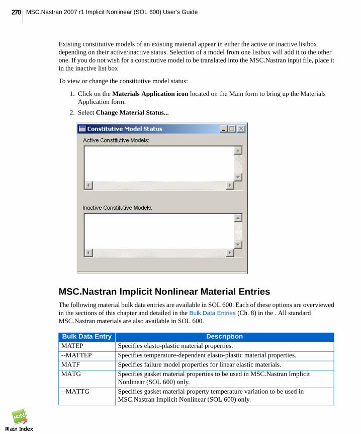
MSC.Nastran 2007 r1 Implicit Nonlinear (SOL 600) User’s Guide270
Existing constitutive models of an existing material appear in either the active or inactive listboxdepending on their active/inactive status. Selection of a model from one listbox will add it to the otherone. If you do not wish for a constitutive model to be translated into the MSC.Nastran input file, place itin the inactive list box
To view or change the constitutive model status:
1. Click on the Materials Application icon located on the Main form to bring up the MaterialsApplication form.
2. Select Change Material Status...
MSC.Nastran Implicit Nonlinear Material EntriesThe following material bulk data entries are available in SOL 600. Each of these options are overviewedin the sections of this chapter and detailed in the Bulk Data Entries (Ch. 8) in the . All standardMSC.Nastran materials are also available in SOL 600.
Bulk Data Entry DescriptionMATEP Specifies elasto-plastic material properties.
--MATTEP Specifies temperature-dependent elasto-plastic material properties.
MATF Specifies failure model properties for linear elastic materials.
MATG Specifies gasket material properties to be used in MSC.Nastran ImplicitNonlinear (SOL 600) only.
--MATTG Specifies gasket material property temperature variation to be used inMSC.Nastran Implicit Nonlinear (SOL 600) only.

271CHAPTER 10Materials
The following sections describe how to model material behavior in MSC.Nastran Implicit Nonlinear.Modeling material behavior consists of both specifying the constitutive models used to describe thematerial behavior and defining the actual material data necessary to represent the material. Directionaldependency can be included for materials other than isotropic materials. Data for the materials can beentered into MSC.Nastran Implicit Nonlinear either directly through the input file or by user subroutines,or material models may be defined in the MSC.Patran Materials Application. Each section of this chapterdiscusses various options for organizing material data for input. Each section also discusses theconstitutive (stress-strain) relation and graphic representation of the models and includesrecommendations and cautions concerning the use of the models.
MATHE Specifies hyperelastic (rubber-like) material properties for nonlinear (large strainand large rotation) analysis in MSC.Nastran Implicit Nonlinear (SOL 600) only.
--MATTHE Specifies temperature-dependent properties of hyperelastic (rubber-like)materials (elastomers) in MSC.Nastran Implicit Nonlinear (SOL 600) only.
MATED Specifies damage model properties for hyperelastic materials in MSC.NastranImplicit Nonlinear (SOL 600) only.
MATORT Specifies elastic orthotropic material properties for 3-dimensional and planestrain behavior for linear and nonlinear analyses in MSC.Nastran ImplicitNonlinear (SOL 600) only.
--MATTORT Specifies temperature-dependent properties of elastic orthotropic materials forlinear and nonlinear analyses used in MSC.Nastran Implicit Nonlinear(SOL 600) only.
MATVE Specifies isotropic visco-elastic material properties in MSC.Nastran ImplicitNonlinear (SOL 600) only.
--MATTVE Specifies temperature-dependent visco-elastic material properties in terms ofThermo-Rheologically Simple behavior in MSC.Nastran Implicit Nonlinear(SOL 600) only.
MATVP Specifies viscoplastic or creep material properties to be used for quasi-staticanalysis in MSC.Nastran Implicit Nonlinear (SOL 600) only.
Bulk Data Entry Description

MSC.Nastran 2007 r1 Implicit Nonlinear (SOL 600) User’s Guide272
Linear ElasticMSC.Nastran Implicit Nonlinear is capable of handling problems with any combination of isotropic,orthrotropic, or anisotropic linear elastic material behavior.
The linear elastic model is the model most commonly used to represent engineering materials. Thismodel, which has a linear relationship between stresses and strains, is represented by Hooke’s Law.Figure 10-1 shows that stress is proportional to strain in a uniaxial tension test. The ratio of stress to strainis the familiar definition of modulus of elasticity (Young’s modulus) of the material.
E (modulus of elasticity) = (axial stress)/(axial strain) (10-1)
Figure 10-1 Uniaxial Stress-Strain Relation of Linear Elastic Material
Experiments show that axial elongation is always accompanied by lateral contraction of the bar. The ratiofor a linear elastic material is:
= (lateral contraction)/(axial elongation) (10-2)
This is known as Poisson’s ratio. Similarly, the shear modulus (modulus of rigidity) is defined as:
(shear modulus) = (shear stress)/(shear strain) (10-3)
A Poisson’s ratio of 0.5, which would be appropriate for an incompressible material, can be used for thefollowing elements: Herrmann, plane stress, shell, truss, or beam. A Poisson’s ratio which is close (butnot equal) to 0.5 can be used for constant dilation elements and reduced integration elements in situationswhich do not include other severe kinematic constraints. Using a Poisson’s ratio close to 0.5 for all otherelements usually leads to behavior that is too stiff. A Poisson’s ratio of 0.5 can also be used with theupdated Lagrangian formulation in the multiplicative decomposition framework using the standarddisplacement elements. In these elements, the treatment for incompressibility is transparent.
Str
ess
Strain
E
1
v
G

273CHAPTER 10Materials
Isotropic MaterialsMost linear elastic materials are assumed to be isotropic (their elastic properties are the same in alldirections). For an isotropic material, every plane is a plane of symmetry and every direction is an axisof symmetry. It can be shown that for an isotropic material:
(10-4)
The shear modulus can be easily calculated if the modulus of elasticity and Poisson’s ratio are known.
Specifying Isotropic Material Entries
Isotropic material models are designated with the MAT1 Bulk Data entry in the MSC.Nastran Input File.
References• MAT1, 1613 of the MSC.Nastran Quick Reference Guide.
MSC.Patran Materials Application Input Data
To define an isotropic material in MSC.Patran:
1. From the Materials Application form, set the Action>Object>Method combination toCreate>Isotropic>Manual Input.
2. Click Input Properties...
Isotropic linear elastic material models require the following material data via the Input Options subformon the Materials Application form.
Entry Description
MAT1 Defines the material properties for linear isotropic materials.
Isotropic-Linear Elastic Description
Elastic Modulus Defines the elastic modulus. This property is generally required. May varywith temperature via a defined material field.
Poisson’s Ratio Defines the Poisson’s ratio. This property is generally required. May varywith temperature via a defined material field.
Density Defines the mass density. This property is optional.
Coefficient of ThermalExpansion
Defines the coefficient of thermal expansion. This property is optional.May vary with temperature via a defined material field.
Reference Temperature Defines the stress free temperature. This property is optional. Whendefining temperature dependent properties, this is the referencetemperature from which values will be extracted or interpolated.
G E 2 1 v+( )( )⁄=
G E v

MSC.Nastran 2007 r1 Implicit Nonlinear (SOL 600) User’s Guide274
The material density, used to define the mass of the structure, and the damping value are used in dynamicloadings, while the expansion coefficient is used to identify the thermal strains.
Orthotropic MaterialsAn orthotropic material has three mutually orthogonal planes of symmetry. With respect to a coordinatesystem parallel to these planes, the constitutive law for this material is given by the following moregeneral form of Hooke’s Law:
3-D Orthotropic
Due to symmetry of the compliance matrix, E11 = E22 , E22 = E33 , and E33 =
E11 . Using these relations, a general orthotropic material has nine independent constants:
E11, E22, E33, , , , G12, G23, G31
These nine constants must be specified in constructing the material model.
2-D Orthotropic
Orthotropic material models can be used with 2-D elements, such as plane stress, plane strain, andaxisymmetric elements. For example, the orthotropic stress-strain relationship for a plane stresselement is:
(10-5)
ε11
ε22
ε33
γ12
γ23
γ13
1 E1( )⁄ υ12( ) E1( )⁄– υ13( ) E1( )⁄– 0 0 0
υ12–( ) E1( )⁄ 1 E2( )⁄ υ23–( ) E2( )⁄ 0 0 0
υ13–( ) E1( )⁄ υ23–( ) E2( )⁄ 1 E3( )⁄ 0 0 0
0 0 0 1 G12( )⁄ 0 0
0 0 0 0 1 G23( )⁄ 0
0 0 0 0 0 1 G13( )⁄
σ11
σ22
σ33
τ12
τ23
τ13
=
ν21 ν12 ν32 ν23 ν13
ν31
ν12 ν23 ν31
Note: The inequalities E22 > E33, E11 > E22, and E33 > E11 must be satisfied in
order for the orthotropic material to be stable. This is checked by MSC.NastranImplicit Nonlinear.
ν23 ν12 ν31
C1
1 ν12ν21–( )-------------------------------
E1 ν21E1 0
ν12E2 E2 0
0 0 1 ν12ν21–( )G
=

275CHAPTER 10Materials
Specifying Orthotropic Material Entries
2-D and 3-D othrotropic materials are characterized in MSC.Nastran using the following bulkdata entries.
References• MAT3, 1619 of the MSC.Nastran Quick Reference Guide.• MAT8, 1624of the MSC.Nastran Quick Reference Guide.• MATORT (SOL 600), 1572 of the MSC.Nastran Quick Reference Guide.
MSC.Patran Materials Application Input Data
To define an orthotropic material in MSC.Patran:
1. From the Materials Application form, set the Action>Object>Method combination to Create>2Dor 3D Orthotropic>Manual Input.
2. Click Input Properties...
The required properties for orthotropic linear elastic material models vary based on dimension, elementtype, and thermal dependencies. 3-D orthotropic material models require the following material data(2-D requires a reduced set) via the Input Properties subform on the Materials Application form.
Entry Description
MAT3 Defines the material properties for linear orthotropic materials used by theCTRIAX6 element entry.
MAT2
MAT8
Defines the material property for an orthotropic material for solids andisoparametric shell elements.
MATORT Specifies elastic orthotropic material properties for three-dimensional andplane strain behavior for linear and nonlinear analyses in MSC.Nastran ImplicitNonlinear (SOL 600) only in a more general way than MAT2 or MAT8.
Orthotropic-Linear Elastic Description
Elastic Modulus 11/22/33 Defines the elastic moduli in the element’s coordinate system. This isrequired data. May vary with temperature via a defined material field.
Poisson’s Ratio 12/23/31 Defines the Poisson’s ratios relative to the element’s coordinatesystem. This is required data. May vary with temperature via a definedmaterial field.
Shear Modulus 12/23/31 Defines the shear moduli relative to the element’s coordinate system.This is required data. May vary with temperature via a definedmaterial field.

MSC.Nastran 2007 r1 Implicit Nonlinear (SOL 600) User’s Guide276
Anisotropic MaterialsAnisotropic material exhibits different elastic properties in different directions. The significant directionsof the material are labeled as preferred directions, and it is easiest to express the material behavior withrespect to these directions.
The stress-strain relationship for an anisotropic linear elastic material can be expressed as
(10-6)
The values of (the stress-strain relation) and the preferred directions (if necessary) must be defined
for an anisotropic material.
Specifying Anisotropic Material Entries
Anisotropic materials are characterized in MSC.Nastran using the following bulk data entries.
References• MAT2, 1617 of the MSC.Nastran Quick Reference Guide.
MSC.Patran Materials Application Input Data
To define anisotropic material in MSC.Patran:
1. From the Materials Application form, set the Action>Object>Method combination to Create>2Dor 3D Anisotropic>Manual Input.
2. Click Input Properties...
Coefficient of ThermalExpansion 11/22/33
Defines the coefficients of thermal expansion relative to the element’scoordinate system. These properties are optional. May vary withtemperature via a defined material field.
Reference Temperature Defines the stress free temperature which is an optional property.When defining temperature dependent properties, this is the referencetemperature from which values will be extracted or interpolated.
Density Defines the mass density which is an optional property.
Entry Description
MAT2 Defines the material properties for linear anisotropic materials for two-dimensional elements.
Orthotropic-Linear Elastic Description
σi j Cijk lεkl=
Cijkl

277CHAPTER 10Materials
Anisotropic linear elastic material models require the following material data via the Input Propertiessubform on the Materials Application form.
Anisotropic-Linear Elastic Description
Stress-Strain Matrix, Cij Defines the upper right portion of the symmetric stress-strain matrixrelative to the element’s coordinate system.
Coefficient of ThermalExpansion
Defines the coefficients of thermal expansion relative to the element’scoordinate system. They are optional properties.
Reference Temperature Defines the stress free temperature which is an optional property.When defining temperature dependent properties, this is the referencetemperature from which values will be extracted or interpolated.
Density Defines the mass density which is an optional property.

MSC.Nastran 2007 r1 Implicit Nonlinear (SOL 600) User’s Guide278
Nonlinear Elastic
Hypoelastic - IsotropicThe hypoelastic model is able to represent a nonlinear elastic (reversible) material behavior. For thisconstitutive theory, MSC.Nastran Implicit Nonlinear assumes that
(10-7)
where is a function of the mechanical strain and is a function of the temperature.
The stress and strains are true stresses and logarithmic strains, respectively, when used in conjunctionwith the updated Lagrange and large displacement options.
When used in conjunction with the large displacement option only, Equation (10-7) is expressed as
(10-8)
where are the Green-Lagrangian strain and second Piola-Kirchhoff stress, respectively.
This model can be used with any stress element, including Herrmann formulation elements.
The tensors and may be defined by user subroutine HYPELA. In order to provide an accurate
solution, should be a tangent stiffness evaluated at the beginning of the iteration. In addition, the totalstress should be defined as its exact value at the end of the increment. This allows the residual loadcorrection to work effectively.
In user subroutine HYPELA2, besides the functionality of HYPELA, additional information is available
regarding the kinematics of deformation. In particular, the deformation gradient ( ), rotation tensor ( ),
and the eigenvalues ( ) and eigenvectors ( ) to form the stretch tensor ( ) are also provided. Thisinformation is available only for the continuum elements namely: plane strain, generalized plane strain,plane stress, axisymmetric, axisymmetric with twist, and three-dimensional cases.
Hyperelastic - IsotropicHyperelastic models are specified using either the MATHP or MATHE bulk data entries and are used todescribe the behavior of materials that exhibit elastic response up to large strains, such as rubber, solidpropellant, and other elastomeric materials. These materials are described in terms of a “strain energypotential”, U, which defines the strain energy stored in the material per unit of volume in the initialconfiguration as a function of the strain at that point in the material.
Elastomeric materials are elastic in the classical sense. Upon unloading, the stress-strain curve is retracedand there is no permanent deformation. Elastomeric materials are initially isotropic. Figure 10-2 shows atypical stress-strain curve for an elastomeric material.
σ· i j Li jk lε·kl
gi j+=
L g
S·i j Li jk lE
·kl
gi j+=
E S,
L g
L
F R
λ N U

279CHAPTER 10Materials
Figure 10-2 A Typical Stress-Strain Curve for an Elastomeric Material
Calculations of stresses in an elastomeric material requires an existence of a strain energy function whichis usually defined in terms of invariants or stretch ratios. Significance and calculation of these kinematicquantities is discussed next.
Characteristics of Elastomeric Materials
Most solid rubberlike materials are nearly incompressible: their bulk modulus is several orders ofmagnitude larger than their shear modulus. For applications where the material is not highly confined,the assumption that the material is fully incompressible is usually a good approximation. In cases wherethe material is highly confined (such as in an O-ring), modeling the compressibility can be important forobtaining accurate results. In either case, the use of “hybrid” (mixed formulation) elements isrecommended for this type of material in all but plane stress cases.
Elastomeric foams on the other hand are elastic but very compressible.
Elastomeric materials are considered to be isotropic in nature with random orientation of the longchain molecules.
Strain Energy Potential and Representative Models
Calculations of stresses in an elastomeric material requires an existence of a strain energy function whichis usually defined in terms of invariants or stretch ratios.
In the rectangular block in Figure 10-3, , , and are the principal stretch ratios along the edges
of the block defined by
(10-9)
σ,S
tres
s
ε, Strain
100%
λ1 λ2 λ3
λi Li ui+( ) Li⁄=

MSC.Nastran 2007 r1 Implicit Nonlinear (SOL 600) User’s Guide280
Figure 10-3 Rectangular Rubber Block
In practice, the material behavior is (approximately) incompressible, leading to the constraint equation
the strain invariants are defined as
(10-10)
Depending on the choice of configurations, for example, reference (at ) or current ( ),you obtain total or updated Lagrange formulations for elasticity. The kinematic measures for the twoformulations are discussed next.
Total Lagrangian Formulation
The strain measure is the Green-Lagrange strain defined as:
(10-11)
where is the right Cauchy-Green deformation tensor defined as:
(10-12)
in which is the deformation gradient (a two-point tensor) written as:
(10-13)
L3
λ2L2
L2
L1
λ1L1 Undeformed
Deformed
λ3L3
λ1λ2λ3 1=
I1 λ12 λ
22 λ
32+ +=
I2 λ1
2λ2
2 λ2
2λ32 λ
3
2λ1
2+ +=
I3 λ12λ
22λ
32
=
t 0= t n 1+=
Eij12--- Cij δi j–( )=
Cij
Cij FkiFkj=
Fkj
Fkj
∂xk
∂Xj---------=

281CHAPTER 10Materials
The Jacobian is defined as:
(10-14)
Thus, the invariants can be written as:
(10-15)
in which is the permutation tensor. Also, using spectral decomposition theorem,
(10-16)
in which the stretches are the eigenvalues of the right Cauchy-Green deformation tensor, and
the eigenvectors are .
Updated Lagrange Formulation
The strain measure is the true or logarithmic measure defined as:
(10-17)
where the left Cauchy-Green or finger tensor is defined as:
(10-18)
Thus, using the spectral decomposition theorem, the true strains are written as:
(10-19)
where is the eigenvectors in the current configuration. It is noted that the true strains can also be
approximated using first Padé approximation, which is a rational expansion of the tensor, as:
(10-20)
J
J λ1λ2λ3 det Cij( )12---
= =
I1 Cii=
I2
CijCi j Cii( )2–( )2
------------------------------------------=
I316--- eijkepqrCipCjqCkr det Cij( )= =
(implied sum on i)
eijk
Cij λA2
NiA
NjA
=
λA2
Cij
NiA
εi j12--- ln bij=
bij
bi j FikFjk=
εi j12--- λAln( )ni
A njA=
niA
εi j 2 Vi j δi j–( ) Vij δi j+( ) 1–=

MSC.Nastran 2007 r1 Implicit Nonlinear (SOL 600) User’s Guide282
where a polar decomposition of the deformation gradient is done into the left stretch tensor and
rotation tensor as:
The Jacobian is defined as:
(10-21)
and the invariants are now defined as:
(10-22)
It is noted that either Equation (10-15) or Equation (10-22) gives the same strain energy since it is scalarand invariant. Also, to account for the incompressibility condition, in both formulations, the strain energyis split into deviatoric and volumertic parts as:
(10-23)
Mooney-Rivlin Model
The generalized Mooney-Rivlin model for nearly-incompressible elastomeric materials is written as:
(10-24)
where and are the first and second deviatoric invariants.
Jamus-Green-Simpson Model
A particular form of the generalized Mooney-Rivlin model, namely the third order deformation (tod)model, is implemented in MSC.Nastran Implicit Nonlinear (SOL 600). This is one of the few placeswhere the formulation for SOLs 106 and 129 may be more appropriate because they can use up to fifthorder terms. However, the Ogden formulation (below) is usually better for large strain behavior than eventhe fifth order Mooney-Rivlin.
(10-25)
Fij Vi j
Rij
Fij VikRkj=
J
J λ1λ2λ3 det bij( )12---
= =
I1 bii=
I212--- bijbi j bi i( )2
–( )=
I316--- eijkepqrbipbjqbkr det bij( )= =and
W Wdeviatoric Wvolumetric+=
Wdeviator icgmr
Cmn I1 3–( )mI2 3–( )n
n 1=
N
∑m 1=
N
∑=
I1 I2
Wdevratorictod
C10 I1 3–( ) C01 I2 3–( ) C11 I1 3–( ) I2 3–( ) C20 I1 3–( )2 C30 I1 3–( )3+ + + +=

283CHAPTER 10Materials
where is the deviatoric third order deformation form strain energy function,
are material constants obtained from experimental data.
Simpler and popular forms of the above strain energy function are obtained as:
(10-26)
Ogden Model
The form of strain energy for the Ogden model in MSC.Nastran Implicit Nonlinear is,
(10-27)
where are the deviatoric stretch ratios while , , and are the
material constants obtained from the curve fitting of experimental data.
The Ogden model is usually applied to slightly compressible materials. If no bulk modulus is given, it istaken to be virtually incompressible. This model is different from the Mooney model in several respects.The Mooney material model is with respect to the invariants of the right or left Cauchy-Green straintensor and implicitly assumes that the material is incompressible. The Ogden formulation is with respectto the eigenvalues of the right or left Cauchy-Green strain, and the presence of the bulk modulus impliessome compressibility. Using a two-term series results in identical behavior as the Mooney mode if:
, , , and
Arruda-Boyce Model
In the Arruda-Boyce strain energy model, the underlying molecular structure of elastomer is representedby an eight-chain model to simulate the non-Gaussian behavior of individual chains in the network. The
two parameters, and ( is the chain density, is the Botzmann constant, is the temperature,
and is the number of statistical links of length l in the chain between chemical crosslinks) representinginitial modules and limiting chain extensibility and are related to the molecular chain orientation thusrepresenting the physics of network deformation.
As evident in most models describing rubber deformation, the strain energy function constructed byfitting experiment data obtained from one state of deformation to another fails to accurately describe thatdeformation mode. The Arruda-Boyce model ameliorates this defect and is unique since the standardtensile test data provides sufficient accuracy for multiple modes of deformation.
Wdeviatoric
tod
C10 C01 C11 C20 C30, , , ,
Wdeviatoricmr
C10 I1 3–( ) C01 I2 3–( )+= Mooney-Rivlin
Wdeviatoricnh
C10 I1 3–( )= Neo-Hookean
Wdeviator icogden µk
αk------ λ1
αkλ2
αkλ3
αk3–+ +
k 1=
N
∑=
λ i
αkJ
αk3
-------–λi
αk= Cmn µk αk
µ1 2C10= α1 2= µ2 2C01–= α2 2–=
nkΘ N n k ΘN

MSC.Nastran 2007 r1 Implicit Nonlinear (SOL 600) User’s Guide284
Figure 10-4 Eight Chain Network in Stretched Configuration
The model is constructed using the eight chain network as follows:
Consider a cube of dimension with an unstretched network including eight chains of length
, where the fully extended chain has an approximate length of Nl. A chain vector from the
center of the cube to a corner can be expressed as:
(10-28)
Using geometrical considerations, the chain vector length can be written as:
(10-29)
and
(10-30)
Using statistical mechanics considerations, the work of deformation is proportional to the entropy changeon stretching the chains from the unstretched state and may be written in terms of the chain length as:
(10-31)
where is the chain density and is a constant. is an inverse Langevin function correctly accountsfor the limiting chain extensibility and is defined as:
(10-32)
λ2α0
λ3α0
λ1α0
C1
k
j
i
α0
r0 Nl=
C1
α0
2------ λ1 i
α0
2------ λ2 j
α0
2------ λ3 k+ +=
rchain1
3------- Nl λ1
2 λ22 λ3
2+ +( )1 2⁄=
λchain
rchain
r0------------ 1
3------- I1( )1 2⁄
= =
W nkΘNrchain
Nl------------ β ln
ββsinh
-------------- ΘC–+=
n C β
β L 1–rchain
Nl------------ =

285CHAPTER 10Materials
where Langevin is defined as:
(10-33)
With Equation (10-30) through Equation (10-33), the Arruda-Boyce model can be written
(10-34)
Gent Model
Also, using the notion of limiting chain extensibility, Gent proposed the following constitutive relation:
(10-35)
where
(10-36)
The constant is independent of molecular length and, hence, of degree of crosslinking. The model
is attractive due to its simplicity, but yet captures the main behavior of a network of extensible moleculesover the entire range of possible strains.
The volumetric part of the strain energy is for all the rubber models in MSC.Nastran ImplicitNonlinear is:
(10-37)
when is the bulk modulus. It can be noted that the particular form of volumetric strain energy is chosensuch that:
1. The constraint condition is satisfied for incompressible deformations only; for example:
(10-38)
ℑ β( ) β 1β---–coth=
WdevArruda-Boyce
nkΘ 12--- I1 3–( ) 1
20N---------- I1
2 9–( ) 11
1050N2
------------------- I13 27–( )+ +=
19
7000N3
------------------- I14 81–( ) 519
673750N4
------------------------- I15 243–( ) ]+ +
WdevGent EIm–
6-------------
Im
Im I1*–
------------------log=
I1* I1 3–=
EIm
Wvolumetric9K2
------- J
13---
1–
2
=
K
f I3( )> 0 if I3 0>
0= if I3 1=
< 0 if I3 0<

MSC.Nastran 2007 r1 Implicit Nonlinear (SOL 600) User’s Guide286
2. The constraint condition does not contribute to the dilatational stiffness.
This yields the constraint function as:
(10-39)
upon substitution of Equation (10-39) in Equation (10-35) and taking the first variation of the variationalprinciple, you obtain the pressure variable as:
(10-40)
The equation has a physical significance in that for small deformations, the pressure is linearly related to
the volumetric strains by the bulk modulus .
The discontinuous or continuous damage models discussed in the models section on damage can beincluded with the generalized Mooney-Rivlin, Ogden, Arruda-Boyce, and Gent models to simulateMullins effect or fatigue of elastomers when using the updated Lagrangian approach. In the totalLagrangian framework however, this is available for the Ogden model only.
Foam Model
Sometimes elastomeric materials show large volumetric deformations. For this type of behavior, themodels discussed above are not appropriate. Instead, the foam model expressed by:
(10-41)
should be used. In contrast to the Ogden model, the first part of the foam strain energy function is notpurely deviatoric. The material constants provide additional flexibility to describe the material
behavior also for a large amount of compressibility.
Updated Lagrange Formulation for Nonlinear Elasticity
The Mooney-Rivlin, Ogden, Arruda-Boyce, Gent and Foam models may be used either in the totalLagrange or updated Lagrange framework. This is selected using the PARAM,MARUPDAT. For planestress analysis the total Lagrange procedure will always be used.
The updated Lagrangian rubber elasticity capability can be used in conjunction with both continuous aswell as discontinuous damage models. Thermal, as well as viscoelastic, effects can be modeled with thecurrent formulation. While the Mooney model can account for the temperature dependent materialproperties, the Ogden model does not support the temperature dependence at this time. The singularityratio of the system is inversely proportional to the order of bulk modulus of the material due to thecondensation procedure.
f I3( ) 3 I3
16---
1–
=
p 3K J
13---
1–
=
K
Wµn
αn------ λ1
αn λ2
αn λ3
αn3–+ +
µn
βn------ 1 J
βn–
n 1=
N
∑+
n 1=
N
∑=
βn

287CHAPTER 10Materials
A consistent linearization has been carried out to obtain the tangent modulus. The singularity for the caseof two- or three-equal stretch ratios is analytically removed by application of L’Hospital’s rule. Thecurrent framework with an exact implementation of the finite strain kinematics along with the split ofstrain energy to handle compressible and nearly incompressible response is eminently suitable forimplementation of any nonlinear elastic as well as inelastic material models. In fact, the finite
deformation plasticity model based on the multiplicative decomposition, is implementedin the same framework.
To simulate elastomeric materials, incompressible element(s) are used for plane strain, axisymmetric,and three-dimensional problems for elasticity in total Lagrangian framework. These elements can beused with each other or in combination with other elements. For plane stress, beam, plate or shellanalysis, conventional elements can be used. For updated Lagrangian elasticity, both conventionalelements (as well as Herrmann elements) can be used for plane strain, axisymmetric, and three-dimensional problems.
Experimental Determination of Hyperelastic Material Parameters
In order to determine the material parameters to be used, like Mooney coefficients, Ogden moduli,relaxation times, etc., experiments must be carried out. In this section, the laboratory tests of which datacan be used to fit the material parameters will be described. Once the test data is available theExperimental Data Fitting module in MSC.Patran can be used to calculate appropriate coefficient values.
For a homogeneous material, homogeneous deformation modes suffice to characterize the materialconstants. MSC.Nastran Implicit Nonlinear accepts test data from the following deformation modes:
• Uniaxial tension and compression.• Biaxial tension and compression.• Planar tension and compression (also known as pure shear).• Simple Shear• Volumetric tension and compression
F FeF
θF
p=

MSC.Nastran 2007 r1 Implicit Nonlinear (SOL 600) User’s Guide288
Figure 10-5 Test Data
Uniaxial Test
Probably the most popular test is the uniaxial test (see Figure 10-6). This test can be used in tension aswell as in compression, both for incompressible and (slightly) compressible elastomeric materials. The
1
2
3
1
2
3
1
2
3
1
2
3
Uniaxial Test Data
Biaxial Test Data
Planar Test Data
Volumetric Test Data

289CHAPTER 10Materials
shape of the specimen used in compression will usually be less slender than the shape used in tension.Within the region indicated by the dashed line, the state of deformation will be homogeneous, where thedeformation can be described by:
, (10-42)
while the corresponding engineering stresses are given by:
, (10-43)
in which is the applied force and is the cross sectional area of the undeformed specimen in the
- -plane, within the region indicated by the dashed line.
Figure 10-6 Uniaxial (Tensile) Test
Necessary input for the curve fitting program in MSC.Patran consists of at least engineering strain ( )
versus engineering stress ( ) data points. In case of (slightly) compressible materials, information
about the volume changes is also needed. This data can be given either in terms of the area ratio or thevolume ratio. The area ratio is defined by the current cross sectional area over the original cross
sectional area . Similarly, the volume ratio is defined by the current volume over the undeformed
volume . Notice that the volume ratio and the area ratio are related by:
If, for a particular elastomeric material, both a tensile and a compression test have been performed, allthe data points should be collected into one data file. The layout of a data file containing uniaxial testdata is given in the figure below. The columns may be separated by either spaces or commas. For (nearly)incompressible material behavior, the third column can be omitted.
λ1 λ 1 e11+= = λ2 λ3 J λ⁄= =
σ11 σ FA0-------= = σ22 σ33 0= =
F A0
E2 E3
E1E3
E2
F F
e11
σ11
A
A0 V
V0
VV0------- J
AA0------- 1 e11+( )= =

MSC.Nastran 2007 r1 Implicit Nonlinear (SOL 600) User’s Guide290
Figure 10-7 Layout of Data File for a Uniaxial Test
Equi-Biaxial Test
The equi-biaxial tensile test outlined in Figure 10-8 can be used to obtain, within the region indicated bythe dashed line, a homogeneous state of deformation defined by:
Figure 10-8 Equi-biaxial (Tensile) Test
, (10-44)
with corresponding engineering stresses:
, (10-45)
e11 σ11 A A0⁄ e11 σ11 V V0⁄
or
F
F
F F
E1E3
E2
λ1 λ2 λ 1 e11+ 1 e22+= = = = λ3 J λ2⁄=
σ11 σ22 σ FA0-------= = = σ33 0=

291CHAPTER 10Materials
with being the original cross sectional area of the elastomeric sheet in the direction perpendicular to
the applied forces, which is assumed to be the same in the - -plane and the - -plane.
For compressible elastomers, volumetric information is needed. For the equi-biaxial test, this can begiven in terms of a thickness ratio or, similar to the uniaxial test, a volume ratio. The thickness ratio isdefined as the current sheet thickness over the original sheet thickness . The relation between the
thickness ratio and the volume ratio is:
(10-46)
The layout of a data file for an equi-biaxial tensile test is given in Figure 10-8.
Planar Shear Test
A state of planar shear, also sometimes called pure shear, can be obtained by clamping and stretching anelastomeric rectangular sheet of material, as indicated in Figure 10-9.
Figure 10-9 Planar Shear Test
Except for the vicinity of the free edges and the clamps, the state of strain can be found to be substantiallyuniform, according to:
, , (10-47)
where the known stress components are given by:
, (10-48)
A0
E1 E3 E2 E3
t t0
VV0------- J
tt0---- 1 e11+( )2
= =
FF
E1E3
E2
λ1 λ 1 e11+= = λ2 1= λ3Jλ---=
σ11 σ FA0-------= = σ33 0=

MSC.Nastran 2007 r1 Implicit Nonlinear (SOL 600) User’s Guide292
in which is the cross sectional area of the undeformed specimen in the - -plane. Notice that the
engineering strain is zero, but that the corresponding engineering stress depends on the material
behavior.
(10-49)
(10-50)
Simple Shear Test
A test which, compared to the above mentioned tests, leads to a more complex kinematic description, isthe simple shear test (see Figure 10-10).Upon introducing the shear strain , the coordinates in thedeformed configuration are given by:
, , (10-51)
which yields for the deformation gradient:
(10-52)
Figure 10-10 Simple Shear Test
Notice that , irrespective of the value of , from which it can be concluded that a simpleshear test is a constant volume test.
A0 E1 E3
e22 σ22
δU TSδλS=
TS λS∂∂
U 2 λS λS3–
–
I1∂∂U
I2∂∂U
+
= =
γ
x1 X1 γX2+= x2 X2= x3 X3=
F1 γ 0
0 1 0
0 0 1
=
2F
E1E3
E2 γatan
det F( ) 1= γ

293CHAPTER 10Materials
Based on Equation (10-51), Equation (10-52) and Figure 10-10, the engineering strain tensor and the rightCauchy-Green strain tensor can be evaluated as:
(10-53)
(10-54)
According to Equation (10-54), the principal stretch ratios follow from the principal values ofand read:
, (10-55)
It can easily be verified that , which again shows that the simple shear test is a constant
volume test. The relevant engineering stress is given by:
(10-56)
with being the cross sectional area of the undeformed specimen in the - -plane.
The layout of a data file containing measurements of a simple shear test is given in Figure 10-11.
Figure 10-11 Layout of Data File for a Simple Shear Test
Volumetric Test
Although a uniaxial, equi-biaxial and planar shear test can be used to obtain information about thevolumetric behavior, for compressible materials an additional volumetric test may be preferable. This isespecially true for slightly compressible materials, since volumetric data from other tests other than avolumetric one may easily be inaccurate (because most of the deformation is deviatoric). Two commonly
e0 γ 2⁄ 0
γ 2⁄ 0 0
0 0 0
=
C1 γ 0
γ 1 γ2+ 0
0 0 1
=
C
λ1 2, 1γ2
2----- γ± 1
γ2
4-----++= λ3 1=
λ1λ2λ3 1=
σ12F
A0-------=
A0 E1 E3
2e12 γ= σ12
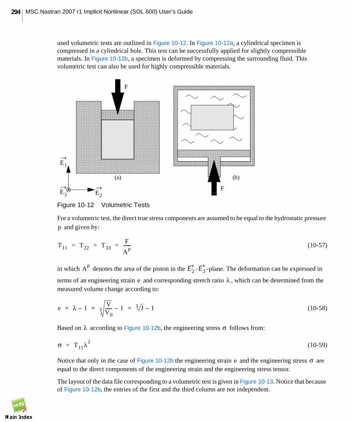
MSC.Nastran 2007 r1 Implicit Nonlinear (SOL 600) User’s Guide294
used volumetric tests are outlined in Figure 10-12. In Figure 10-12a, a cylindrical specimen iscompressed in a cylindrical hole. This test can be successfully applied for slightly compressiblematerials. In Figure 10-12b, a specimen is deformed by compressing the surrounding fluid. Thisvolumetric test can also be used for highly compressible materials.
Figure 10-12 Volumetric Tests
For a volumetric test, the direct true stress components are assumed to be equal to the hydrostatic pressureand given by:
(10-57)
in which denotes the area of the piston in the - -plane. The deformation can be expressed in
terms of an engineering strain and corresponding stretch ratio , which can be determined from themeasured volume change according to:
(10-58)
Based on according to Figure 10-12b, the engineering stress follows from:
(10-59)
Notice that only in the case of Figure 10-12b the engineering strain and the engineering stress areequal to the direct components of the engineering strain and the engineering stress tensor.
The layout of the data file corresponding to a volumetric test is given in Figure 10-13. Notice that becauseof Figure 10-12b, the entries of the first and the third column are not independent.
F
F
F
(a) (b)
E2E3
E1
p
T11 T22 T33F
Ap
-------= = =
Ap
E2 E3
e λ
e λ 1–VV0-------3 1– J3 1–= = =
λ σ
σ T11λ2=
e σ

295CHAPTER 10Materials
Figure 10-13 Layout of Data File for a Volumetric Test
Relaxation Test
The basic feature of a relaxation test is that the force or stress response to a prescribed fixed displacementor deformation is measured as a function of time. A relaxation test for a large strain elastomeric material
is indicated in Figure 10-14. By measuring the force needed for a displacement at different timeintervals, the decay of the strain energy as a function of time can be determined. For linear elasticisotropic material, similar tests can be performed to get information about the shear modulus and/or thebulk modulus as a function of time. In order to properly measure the instantaneous values, applicationof the prescribed displacement should occur sufficiently fast. It should be noted, due to the assumptionintroduced in equation Equation (10-94), that for large strain visco-elastic materials the magnitude of (theinstantaneous value of) the strain energy is not important, since every energy term in the Prony seriesexpansion is related to the instantaneous strain energy using a scalar multiplier. The data does not needto be equispaced in time. Usually, at the beginning of the relaxation experiment the measurements aredone at smaller time intervals than at the end of the experiment.
Figure 10-14 Relaxation Test
If, for linear visco-elastic materials, instead of a relaxation test only a creep test can be performed, thecreep data must be transformed into relaxation data. Converting creep data into relaxation data can bedone using a numerical integration scheme, but is not part of MSC.Nastran Implicit Nonlinear.
e σ V V0⁄
∆u
∆u

MSC.Nastran 2007 r1 Implicit Nonlinear (SOL 600) User’s Guide296
Hyperelastic Foam Properties
Elastomeric foams are cellular solids that have the following primary mechanical characteristics:
• They can deform elastically up to large strain: up to 90% strain in compression. In mostapplications, this is the dominant mode of deformation.
• Their porosity permits very large volumetric changes. This is in contrast to solid rubbers, whichare approximately incompressible.
• Cellular solids are made up of interconnected networks of solid struts or plates which form theedges and faces of cells. Foams are made up of polyhedral cells that pack in three dimensions.The foam cells can either be open (e.g., sponge) or closed (e.g., flotation foam). Commonexamples of elastomeric foam materials are cellular polymers such as cushions, padding, andpackaging materials which utilize the excellent energy absorption properties of foams - for acertain stress level, the energy absorbed by foams is substantially greater than by ordinary stiffelastic materials.
The figure below shows a typical compressive stress-strain curve for elastomeric foam.
Figure 10-15 Typical Compressive Stress-Strain Curve
Three stages can be distinguished during compression:
At small strains (< 5%) the foam deforms in a linear elastic manner, due to cell wall bending.
This is followed by a plateau of deformation at almost constant stress, caused by the elastic buckling ofthe columns or plates which make up the cell edges or walls. In closed cells, the enclosed gas pressureand membrane stretching increase the level and slope of the plateau.
Finally, a region of densification occurs, where the cell walls crush together, resulting in a rapid increaseof compressive stress. Ultimate compressive nominal strains of 0.7 to 0.9 are typical.
The tensile deformation mechanisms for small strains are similar to the compression mechanisms butdiffer for large strains. The figure shows a typical tensile stress-strain curve.
STRAIN
ST
RE
SS
Densification
Plateau: Elastic bucklingof cell walls
Cell wall bending

297CHAPTER 10Materials
Figure 10-16 Typical Tensile Stress-Strain Curve
There are two stages during tension:
At small strains the foam deforms in a linear, elastic manner, due to cell wall bending, similar to thatin compression.
The cell walls rotate and align, resulting in rising stiffness. The walls are substantially aligned at a tensilestrain of about 1/3. Further stretching results in increased axial strains in the walls.
At small strains for both compression and tension, the average experimentally observed Poisson's ratio,ν, of foams is 1/3. At larger strains it is commonly observed that Poisson's ratio is effectively zero duringcompression - the buckling of the cell walls does not result in any significant lateral deformation.However, during tension, ν is nonzero, which is a result of the alignment and stretching of the cell walls.
The manufacture of foams often results in cells with different principal dimensions. This shapeanisotropy results in different loading responses in different directions. However, the foam model doesnot take this kind of initial anisotropy into account.
Determination of Foam Material Parameters
The response of the material is defined by the parameters in the strain energy function, U, so that it isnecessary to determine these parameters to use the foam model. MSC.Patran contains a capabilityfor obtaining the µi, αi and βi for the foam model with up to six terms (N=6) directly from test data. Itis usually best to obtain data from several experiments involving different kinds of deformation, overthe range of strains of interest in the actual application, and to use all of these data to determinethe parameters.
Since the properties of foam materials can vary significantly from one batch to another, all of theexperiments should be performed on specimens taken from the same batch of material or to useMSC.Stocastics in combination with SOL 600.
STRAIN
STR
ESS
Cell wall bending
Cell wall alignment

MSC.Nastran 2007 r1 Implicit Nonlinear (SOL 600) User’s Guide298
Uniaxial, Equibiaxial and Planar Deformations
The deformation modes are characterized in terms of the principal stretches, λi, and the volume ratio, J.The elastomeric foams are not incompressible, so that J = λ1λ2λ3 != 1. The transverse stretches, λ2 and/or
λ3, are independently specified in the test data either as individual values from the measured lateraldeformations or through the definition of an effective Poisson’s ratio.
Uniaxial mode: λ1=λU, λ2=λ3, J=λUλ22
Equibiaxial mode: λ1=λ2=λB, J=λB2λ3
Planar mode: λ1=λP, λ2=1, J=λPλ3
The three deformation modes above use a single form of the nominal stress-stretch relation,
(10-60)
where TL is the nominal stress and LL is the stretch in the direction of loading. Because of thecompressible behavior, the planar mode does not result in a state of pure shear. In fact, if the effectivePoisson’s ratio is zero, planar deformation is identical to uniaxial deformation.
Simple Shear Deformation
Simple shear is described by the deformation gradient
(10-61)
where γ is the shear strain. For this deformation, J=det F =1. A schematic illustration of simple sheardeformation is shown in Figure 10-17.
The nominal shear stress TS is:
(10-62)
where λj= are the principal stretches in the plane of shearing, related to the shear strain, γ, by:
(10-63)
TL λL∂∂U 2
λL-------
µiαi----- λL
αiJ
αiβi––
i 1=
N
∑= =
F1 γ 00 1 00 0 1
=
TS γ∂∂U 2γ
2 λj2
1– γ2
–
--------------------------------------µiαi----- λj
αi1–
i 1=
N
∑
j 1=
2
∑= =
λ1 2, 1γ2
2----- γ 1
γ2
4-----+±+=

299CHAPTER 10Materials
.
Figure 10-17 Simple Shear Test
The stretch in the direction perpendicular to the shear plane is L3=1. The transverse (tensile) stress, TT,developed during simple shear deformation due to the Poynting effect, is
(10-64)
Volumetric Deformation
The volumetric deformation mode consists of all principal stretches being equal,
λ1=λ2=λ3=λV, J=λV3.
The pressure-volumetric ratio relation is
(10-65)
A volumetric compression test is illustrated Figure 10-18.
The pressure exerted on the foam specimen is the hydrostatic pressure of the fluid and the decrease inthe specimen volume is equal to the additional fluid entering the pressure chamber. The specimen issealed against fluid penetration.
2F
E1E3
E2 γatan
TT ε∂∂U
2 λj2
1–
2λj4 λj
2 γ22+( )–
---------------------------------------------µiαi----- λj
αi1–
i 1=
N
∑
j 1=
2
∑= =
p–J∂
∂U 2J---
µiαi----- J
αi3-----
Jαiβi–
–
i 1=
N
∑= =

MSC.Nastran 2007 r1 Implicit Nonlinear (SOL 600) User’s Guide300
Figure 10-18 Volumetric Compression Test Setup
Difference in Compression and Tension Deformation
For small strains (< 5%), foams behave similarly for both compression and tension. However, we haveseen that at large strains, the deformation mechanisms differ for compression (buckling and crushing) andtension (alignment and stretching). Accurate modeling with the FOAM option therefore requires that theexperimental data used to define the material parameters correspond to the dominant deformation modesof the actual problem being analyzed.
If compression dominates in the problem, the pertinent tests are:
• Uniaxial compression.• Simple shear.
• Planar compression (if Poisson’s ratio ).
• Volumetric compression (if Poisson’s ratio ).
If tension dominates, the pertinent tests are:
• Uniaxial tension.• Simple shear.• Biaxial tension (if Poisson’s ratio ).
• Planar tension (if Poisson’s ratio ).
Lateral strain data can also be used to define the compressibility of the foam. Measurement of the lateralstrains may make other tests redundant, e.g., providing lateral strains for a uniaxial test eliminates theneed for a volumetric test. The foam model may not accurately fit Poisson's ratio if it varies significantlybetween compression and tension.
F
F
F
(a) (b)
E2E3
E1
ν 0≠ν 0≠
ν 0≠ν 0≠

301CHAPTER 10Materials
Experimental Data Fitting
Least Squares Fit
The equations derived above for TU, TB, and TS, with the assumption of material incompressibility,allow the material parameters Cij and µi, αi to be determined from the experimentally measured stress-strain relationships in the uniaxial, equibiaxial, and planar loading tests. A least squares fit, whichminimizes the relative error in stress, is used for this purpose. The equation for TS alone will not
determine the constants uniquely. The planar test data input must be augmented by either or both of theother two types of test data to determine the material parameters.
The Ogden potential is linear in the coefficients µi but strongly nonlinear in terms of the exponents αi,thus necessitating use of a nonlinear least squares procedure. For the nominal stress-nominal strain data
pairs, the error measure, E, is minimized by E = sum(i=1to n)(1-Tith/Ti
test2), where Titest is a stress value
from the test data and Tith comes from one of the nominal stress expressions derived above.
The foam parameters µi, αi, βi are determined from the experimentally measured stress-strainrelationships in the various loading tests described above. A least squares fit, which minimizes therelative error in stress, is used for this purpose.
The foam potential is linear in the coefficients µi but strongly nonlinear in terms of the exponents αi and
βi thus necessitating use of a nonlinear least squares procedure. For the n nominal stress-nominal strain
data pairs, the error measure E is minimized by E = sum(i=1to n)(1-Tith/Ti
test2, where Titest is a stress
value from the test data and Tith comes from one of the nominal stress expressions derived above.
Minimizing the relative error in stress implies that the error in slope (modulus) is minimized;minimization of the absolute error would decrease the error at larger strains, at the expense of theaccuracy at small strains.
Alternative Method for Determination of Constants for Moderate Strains
Since the polynomial form with N=1 is very commonly used for cases where the nominal strain is nottoo large, an alternative method of finding the material constants, assuming incompressibility, is to usethe uniaxial test data as follows. The nominal strain in the direction of loading in the uniaxial test isεU=λU-1. Expanding the equation for TB in terms of εU, using the Mooney-Rivlin form, and neglectingterms of higher than second-order in εU, gives
TU=6εU(C10+C01 -(C10+2C01)εU).
This is a parabola: the slope of this curve at the origin (the effective Young’s modulus at zero strain) is
6(C10+C01); this slope, together with the second-order term -6(C10+2C01)εU2, defines the constants C10
and C01.
If compressibility should be modeled, then, under pure pressure loading, the compressible model withN=1 gives, to first-order in the volumetric strain εV=3ε11,

MSC.Nastran 2007 r1 Implicit Nonlinear (SOL 600) User’s Guide302
p=-(2 / D1)εV,
so that, at small nominal strains, the bulk modulus is defined as:
K=(2 / D1)
Hyperelastic Models in MSC.Nastran
Various options are provided for defining the material properties. The first (available in both MSC.Patranand MSC.Nastran) is to give the parameters of the polynomial form and , or the parameters of
the Ogden form and as functions of the temperature. The second is to give the value of N,
and give experimental stress-data for up to four simple tests: uniaxial, equilibrium, planar and, if thematerial is compressible for volumetric compression test. MSC.Nastran Implicit Nonlinear will then
compute the or and the . This method is available for N = 1 and N=2 for the polynomial
form and up to N = 6 for the Ogden form, and does not allow the properties to be temperature dependent.
In either case, you should be careful about defining the or : especially when N > 1, the
behavior at higher strains is strongly sensitive to the values of the or , and unstable material
behavior may result if these values are not correctly defined. When some of the coefficients are stronglynegative, instability at higher strain levels is likely to occur.
Because the properties of rubber-like materials can vary significantly from one sample to another, it isimportant that test data are taken from experiments on the same sample (or samples cut from the samesheet), regardless whether the or are computed by the user or by the built-in method.
This material option can be used by itself, or can be combined with viscoelasticity to define timedependent hyperelastic behavior. It cannot be combined with other material options such as plasticity orcreep. It may be used with the pure displacement formulation elements or with the “hybrid” (mixedformulation) elements. Because elastomeric materials are usually almost completely incompressible,fully integrated pure displacement method elements are not recommended for use with this material,except for plane stress cases. If fully or selectively reduced integration displacement method elementsare used with the almost incompressible form of this material model in anything except plane stressanalysis, a penalty method is used to impose the incompressibility constraint. This can sometimes leadto numerical difficulties, and the fully or selectively reduced integrated “hybrid” formulation elementsare therefore recommended.
Specifying Hyperelastic Material Entries
Nonlinear hyperelastic materials are characterized in MSC.Nastran with the following Bulk Data entries:.
Entry DescriptionMATHP Specifies material properties for use in fully nonlinear (i.e., large strain and
large rotation) hyperelastic analysis of rubber-like materials (elastomers).
MATHE Specifies hyperelastic (rubber-like) material properties for nonlinear (largestrain and large rotation) analysis in (SOL 600) only.
N Aij, Di
N µi αi, , Di
Aij µi αi,[ ] Di
Aij µi αi,[ ]
Aij µi αi,[ ]
Aij µi αi,[ ]

303CHAPTER 10Materials
References• MATHP, 1569 of the MSC.Nastran Quick Reference Guide.• MATHE (SOL 600) (p. 1559) in the MSC.Nastran Quick Reference Guide.
MSC.Patran Materials Application Input Data
To define a hyperelastic material in MSC.Patran:
1. From the Materials Application form, set the Action>Object>Method combination toCreate>Isotropic>Manual Input.
2. Click Input Properties..., and select Hyperelastic from the Constitutive Model pull-down menu.
3. Select Test Data or Coefficients as the Data Type.
4. From the Strain Energy Potential pull-down menu, select a model and enter properties asdescribed below.
Hyperelastic material models require the following material data via the Input Properties subform on theMaterials Application form.
Mooney-Rivlin and James-Green-Simpson
Ogden
Hyperelastic -Mooney/ James Description
Strain Energy Function, C10,C01, C11, C20, C30
Strain energy densities as a function of the strain invariants in thematerial. May vary with temperature via a defined material field.This option consolidates several of the MSC.Marc hyperelasticmaterial models.
Density Defines the mass density which is an optional property.
Coefficient of ThermalExpansion
Defines the instantaneous coefficient of thermal expansion. Thisproperty is optional. May vary with temperature via a definedmaterial field.
Bulk Modulus Defines the Bulk Modulus.
Reference Temperature Defines the reference temperature for the thermalexpansion coefficient.
Hyperelastic-Ogden Description
Bulk Modulus K Defines the Bulk Modulus.
Density Defines the material mass density.
Coefficient of ThermalExpansion
Defines the instantaneous coefficient of thermal expansion. Thisproperty is optional. May vary with temperature via a definedmaterial field

MSC.Nastran 2007 r1 Implicit Nonlinear (SOL 600) User’s Guide304
Foam
Arruda-Boyce
Reference Temperature Defines the reference temperature for the thermal expansioncoefficient.
Modulus k in the Ogden equation.
Exponent k in the Ogden equation.
Hyperelastic-Foam Description
Density Defines the material mass density.
Coefficient of ThermalExpansion
Defines the instantaneous coefficient of thermal expansion. Thisproperty is optional. May vary with temperature via a definedmaterial field
Reference Temperature Defines the reference temperature for the thermalexpansion coefficient.
Modulus n in the Foam equation.
Deviatoric Exponent n in the Foam equation.
Volumetric Exponent n in the Foam equation.
Hyperelastic-Arruda- Boyce Description
NKT Chain density times Boltzmann constant times temperature.
Chain Length Average chemical chain cross length.
Bulk Modulus Defines the Bulk Modulus.
Density This defines the material mass density.
Coefficient of ThermalExpansion
Defines the instantaneous coefficient of thermal expansion. Thisproperty is optional. May vary with temperature via a definedmaterial field
Reference Temperature Defines the reference temperature for the thermalexpansion coefficient.
Hyperelastic-Ogden Description
µk
αk
un
αn
βn

305CHAPTER 10Materials
Gent
ViscoelasticThe material models discussed in previous sections are considered to be time independent. However,rubber materials often show a rate-dependent behavior and can be modeled as viscoelastic materials.Viscoelasticity can be applied:
• To determine the current state of deformation based on the entire time history of loading.
• To characterize small strain and large strain problems.
• With other material options for linear elastic response (small strain) and hyperelastic response(large strain).
• To include temperature dependencies.
• For isotropic, anisotropic, and incompressible materials.
Small Strain Viscoelasticity
In the stress relaxation form, the constitutive relation can be written as a hereditary integral formulation
(10-66)
The functions are called stress relaxation functions. They represent the response to a unit applied
strain and have characteristic relaxation times associated with them. The relaxation functions formaterials with a fading memory can be expressed in terms of Prony or exponential series.
(10-67)
Hyperelastic-Gent Description
Tensile Modulus Defines standard tension modulus (E).
Maximum 1st Invariant Defines .
Bulk Modulus Defines the Bulk Modulus.
Density This defines the material mass density.
Coefficient of ThermalExpansion
Defines the coefficient of thermal expansion.
Reference Temperature Defines the reference temperature for the thermalexpansion coefficient.
I1*
I1*
I1 3–=
σij t( ) Gijkl t τ–( )dεkl τ( )
dτ-------------------dτ
0
t
∫ Gijkl t( )εkl 0( )+=
Gijkl
Gijkl t( ) Gijkl∞
Gijkln
exp t λn⁄–( )
n 1=
N
∑+=

MSC.Nastran 2007 r1 Implicit Nonlinear (SOL 600) User’s Guide306
in which is a tensor of amplitudes and is a positive time constant (relaxation time). In the
current implementation, it is assumed that the time constant is isotropic. In Equation (10-67),
represents the long term modulus of the material.
The short term moduli (describing the instantaneous elastic effect) are then given by
(10-68)
The stress can now be considered as the summation of the stresses in a generalized Maxwell model(Figure 10-19)
(10-69)
where
(10-70)
(10-71)
Figure 10-19 The Generalized Maxwell or Stress Relaxation Form
For integration of the constitutive equation, the total time interval is subdivided into a number of
subintervals ( ) with time-step . A recursive relation can now be derived
expressing the stress increment in terms of the values of the internal stresses at the start of the
interval. With the assumption that the strain varies linearly during the time interval h, we obtain theincrement stress-strain relation as
Gijkl
nλn
Gi jkl∞
Gijkl0
Gijkl 0( ) Gijkl∞
Gijkln
n 1=
N
∑+= =
σij t( ) σij∞
t( ) σijn
t( )
n 1=
N
∑+=
σij∞
Gijkl∞
εkl t( )=
σijn
Gijkln
exp t τ–( ) λn
⁄–[ ]dεkl τ( )
dτ-------------------dτ
0
t
∫=
E1
η1
q1
ε
E0
τi = ηi/Ei
E2
η2
q2
Ei
ηi
qiηE
tm 1– tm, h tm tm 1––=
σi jn

307CHAPTER 10Materials
(10-72)
where
(10-73)
and
(10-74)
In MSC.Nastran Implicit Nonlinear, the incremental equation for the total stress is expressed in terms ofthe short term moduli (See Equation (10-68)).
(10-75)
Note that the set of equations given by Equation (10-75) can directly be used for both anisotropic andisotropic materials.
Isotropic Viscoelastic Material
For an isotropic viscoelastic material, MSC.Nastran Implicit Nonlinear assumes that the deviatoric andvolumetric behavior are fully uncoupled and that the behavior can be described by a time dependentshear and bulk modules. The bulk moduli is generally assumed to be time independent; however, this isan unnecessary restriction of the general theory.
Both the shear and bulk moduli can be expressed in a series
(10-76)
(10-77)
with short term values given by
(10-78)
∆σij tm( ) Gijkl
∞β
nh( )Gijkl
n
n 1=
N
∑+ ∆εkl αnh( )σij
ntm h–( )
n 1=
N
∑–=
αn h( ) 1 exp h λn
⁄–( )–=
βn
h( ) αn
h( )λn
h⁄=
∆σij tm( ) Gijkl0
1 βn
h( )–{ }Gijkln
n 1=
N
∑– ∆εkl tm( ) αnh( )σij
n
n 1=
N
∑–= tm h–( )
G t( ) G∞
Gn
exp t λdn
⁄–
n 1=
N
∑+=
K t( ) K∞
Kn
exp t λvn⁄–
n 1=
N
∑+=
G0 G∞ Gn
n 1=
N
∑+=

MSC.Nastran 2007 r1 Implicit Nonlinear (SOL 600) User’s Guide308
(10-79)
Let the deviatoric and volumetric component matrices and be given by
The increment set of equations is then given by
(10-80)
and
(10-81)
Note that the deviatoric and volumetric response are fully decoupled.
K0 K∞ Kn
n 1=
N
∑+=
πd πv
πd
4 3⁄ 2– 3⁄ 2– 3⁄ 0 0 0
2– 3⁄ 4 3⁄ 2– 3⁄ 0 0 0
2– 3⁄ 2– 3⁄ 4 3⁄ 0 0 0
0 0 0 1 0 0
0 0 0 0 1 0
0 0 0 0 0 1
=
πv
1 1 1 0 0 0
1 1 1 0 0 0
1 1 1 0 0 0
0 0 0 0 0 0
0 0 0 0 0 0
0 0 0 0 0 0
=
∆σ tm( ) G0
1 βdn
h( )–[ ]Gn
n 1=
Nd
∑–
πd∆ε tm( )=
αdn
h( )σdn
tm h–( )
n 1=
Nd
∑ αvn
h( )σvn
tm h–( )
n 1=
Nv
∑––
K0
1 βvn
h( )–[ ]Kn
n 1=
Nv
∑–
πv∆ε tm( )
∆σdn
tm( ) βdn
h( )Gn
πd∆ε tm( ) αdn
h( )σdn
tm h–( )–=
∆σvn
tm( ) βvn
h( )Kn
πv∆ε tm( ) αvn
h( )σvn
tm h–( )–=

309CHAPTER 10Materials
Note that the algorithm is exact for linear variations of the strain during the increment. The algorithm isimplicit; hence, for each change in time-step, a new assembly of the stiffness matrix is required.
Anisotropic Viscoelastic Material
Equation (10-75) can be used for the analysis of anisotropic viscoelastic materials.
Also, a complete set of moduli (21 components) can be specified in the HOOKVI user subroutine.
Referencing a local coordinate system or use of the ORIENT user subroutine can be used to define a
preferred orientation both for the short time moduli and the amplitude functions .
Incompressible Isotropic Viscoelastic Materials
Incompressible elements in MSC.Nastran Implicit Nonlinear allow the analysis of incompressible andnearly incompressible materials in plane strain, axisymmetric and three-dimensional problems. Theincompressibility of the element is simulated through the use of an perturbed Lagrangian variationalprinciple based on the Herrmann formulation.
The constitutive equation for a material with no time dependence in the volumetric behavior can beexpressed as
(10-82)
(10-83)
The hydrostatic pressure term is used as an independent variable in the variational principle. TheHerrmann pressure variable is now defined in the same way as in the formulation for time independentelastic materials.
(10-84)
The constitutive Equation (10-82) and Equation (10-83) can then be rewritten
(10-85)
Gi jkl0
Gi jkln
∆σij tm( ) 2 Gijkl0
1 βn
h( )–[ ]Gijkln
n 1=
N
∑–
∆εkl tm( ) 13---∆εpp tm( )δkl–=
αn
h( ) σ′ij( )n
tm( )
n 1=
N
∑–13---σkkδij+
∆σpp tm( ) 3K0
∆εpp tm( )=
Hσpp
2G0 1 ν0+( )--------------------------------=
∆σij tm( ) 2Ge
∆εij ν∗Hδij+( ) αn h( ) σ′ij( )ntm h–( )
n 1=
N
∑–=

MSC.Nastran 2007 r1 Implicit Nonlinear (SOL 600) User’s Guide310
where
(10-86)
(10-87)
Large Strain Viscoelasticity
For an elastomeric time independent material, the constitutive equation is expressed in terms of an energy
function . For a large strain viscoelastic material, Simo generalized the small strain viscoelasticitymaterial behavior to a large strain viscoelastic material. The energy functional then becomes
(10-88)
where are the components of the Green-Lagrange strain tensor, internal variables and the
elastic strain energy density for instantaneous deformations. In MSC.Nastran Implicit Nonlinear, it is
assumed that , meaning that the energy density for instantaneous deformations is given by thethird order James Green and Simpson form or the Ogden form.
The components of the second Piola-Kirchhoff stress then follow from
(10-89)
The energy function can also be written in terms of the long term moduli resulting in a different set of
internal variables
(10-90)
where is the elastic strain energy for long term deformations. Using this energy definition, thestresses are obtained from
(10-91)
Ge G0 1 βn h( )Gn–[ ]n 1=
N
∑–=
ν∗ G0
1 ν0
+( ) Ge
1 2ν0
–( )–
3Ge
--------------------------------------------------------------------=
W
ψ EijQi jn
( ) ψ0
Eij( ) Qijn
Eij
n 1=
N
∑– ψIn
Qijn( )
n 1=
N
∑+=
Eij Qi jn
ψ0
ψ0W=
Sij∂ψ
∂Eij---------- ∂ψ0
∂Eij---------- Qij
n
n 1=
N
∑–= =
Tijn
ψ Eij Tijn
,( ) ψ∞ Eij( ) Tijn
Eij
n 1=
N
∑+=
ψ∞
Sij∂ψ∞ E( )
∂Eij-------------------- Tij
n
n 1=
N
∑+=

311CHAPTER 10Materials
Observing the similarity with the equations for small strain viscoelasticity the internal variables can beobtained from a convolution expression
(10-92)
where are internal stresses obtained from energy functions.
(10-93)
Let the total strain energy be expressed as a Prony series expansion
(10-94)
If, in the energy function, each term in the series expansion has a similar form, Equation (10-94) canbe rewritten
(10-95)
where is a scalar multiplier for the energy function based on the short term values.
The stress-strain relation is now given by
(10-96)
(10-97)
(10-98)
Analogue to the derivation for small strain viscoelasticity, a recursive relation can be derived expressingthe stress increment in terms of values of the internal stresses at the start of the increment.
Tijn
S·i jn
0t∫ τ( )exp t τ–( ) λ
n⁄–[ ]dτ=
Sijn
Sijn ∂ψn
∂Eij----------=
ψ ψ∞ ψnexp t λn⁄–( )n 1=
N
∑+=
ψ ψ∞ δnψ0exp t λn⁄–( )n 1=
N
∑+=
δn
Sij t( ) Sij∞
t( ) Tijn
n 1=
N
∑ t( )+=
Sij∂ψ∞
∂Eij----------- 1 δn
n 1=
N
∑– ∂ψ0
∂Eij----------= =
Tijn
δnSij
0t( )exp t τ–( ) λ
n⁄–[ ]dτ
0
t
∫=

MSC.Nastran 2007 r1 Implicit Nonlinear (SOL 600) User’s Guide312
The equations are reformulated in terms of the short time values of the energy function
(10-99)
(10-100)
It is assumed that the viscoelastic behavior in MSC.Nastran Implicit Nonlinear acts only on thedeviatoric behavior.
Viscoelastic Models in MSC.Nastran
MSC.Nastran Implicit Nonlinear has two models that represent viscoelastic materials. The first can bedefined as a Kelvin-Voigt model. The latter is a general hereditary integral approach.
Kelvin-Voigt Model
The Kelvin model allows the rate of change of the inelastic strain to be a function of the total stress andprevious strain.
The Kelvin material behavior (viscoelasticity) is modeled by assuming an additional creep strain ,
governed by
(10-101)
where and may be defined in the user subroutine CRPVIS and the total strain is
(10-102)
(10-103)
(10-104)
(10-105)
(10-106)
(10-107)
∆Sij tm( ) 1 1 βn h( )–
n 1=
N
∑– δn
Si j0
tm( ) Sij0 tm h–( )–{ }=
αnSi jn
tm h–( )n 1=
N
∑–
∆Sij tm( ) βn h( )δn Sij0
tm( ) Sijn
tm h–( )–[ ] αn h( )Sijn
tm h–( )–=
εi jk
ddt-----ε
i jk Aijklσ′
klBijklεkl
k–=
A B
εi j εi je ε
i jp ε
i jc ε
i jk ε
i jth+ + + +=
εi jth
= thermal strain components
εi je = elastic strain components (instantaneous response)
εi jp
= plastic strain components
εi jc = creep strains defined via the CRPLAW and VSWELL user subroutines
εi jk = Kelvin model strain components as defined above

313CHAPTER 10Materials
The CRPVIS user subroutine is called at each integration point of each element when the Kelvin modelis used.
Use the NLPARM option and set a nonzero time increment to define the time step and to set the tolerancecontrol for the maximum strain in any increment.
This option allows Maxwell models to be included in series with the Kelvin model.
Hereditary Integral Model
The stress-strain equations in viscoelasticity are not only dependent on the current stress and strain state(as represented in the Kelvin model), but also on the entire history of development of these states. Thisconstitutive behavior is most readily expressed in terms of hereditary or Duhamel integrals. Theseintegrals are formed by considering the stress or strain build-up at successive times. Two equivalentintegral forms exist: the stress relaxation form and the creep function form. In MSC.Nastran ImplicitNonlinear, the stress relaxation form is used.
The viscoelasticity option in MSC.Nastran Implicit Nonlinear can be used for both the small strain andlarge strain Mooney, Ogden, Arruda Boyce, and Gent material stress-relaxation problems. A descriptionof these models is as follows:
Experimental Determination of Viscoelastic Material Parameters
The free energy function versus time data being used for large strain viscoelasticity can be generated byfitting experimental data provided the following two tests are done:
1. Standard quasi-static tests (tensile, planar-shear, simple-shear, equi-biaxial tension, volumertic)
to determine the elastomer free energy constants.
2. Standard relaxation tests to obtain stress versus time.
Temperature Dependence of Viscoelastic Materials
The rate processes in many viscoelastic materials is known to be highly sensitive to temperature changes.Such temperature-dependent properties cannot be neglected in the presence of any appreciabletemperature variation. For example, there is a large class of polymers which are adequately representedby linear viscoelastic laws at uniform temperature. These polymers exhibit an approximate translationalshift of all the characteristic response functions with a change of temperature, along a logarithmic timeaxis. This shift occurs without a change of shape. These temperature-sensitive viscoelastic materials arecharacterized as Thermo-Rheologically Simple.
A “reduced” or “pseudo” time can be defined for the materials of this type and for a given temperaturefield. This new parameter is a function of both time and space variables. The viscoelastic law has thesame form as one at constant temperature in real time. If the shifted time is used, however, thetransformed viscoelastic equilibrium and compatibility equations are not equivalent to the correspondingelastic equations.
In the case where the temperature varies with time, the extended constitutive law implies a nonlineardependence of the instantaneous stress state at each material point of the body upon the entire local
W0

MSC.Nastran 2007 r1 Implicit Nonlinear (SOL 600) User’s Guide314
temperature history. In other words, the functionals are linear in the strains but nonlinear inthe temperature.
The time scale of experimental data is extended for Thermo-Rheologically Simple materials. Allcharacteristic functions of the material must obey the same property. The shift function is a basic propertyof the material and must be determined experimentally. As a consequence of the shifting of themechanical properties data parallel to the time axis, the values of the zero and infinite frequency complexmoduli do not change due to shifting. Hence, elastic materials with temperature-dependentcharacteristics neither belong to nor are consistent with the above hypothesis for the class ofThermo-Rheologically Simple viscoelastic solids.
In addition to the Thermo-Rheologically Simple material behavior variations of initial stress-strain
moduli , the temperature of the other mechanical properties (coefficient of thermal expansion, etc.)
due to changes in temperature can be specified.
Note, however, that only the instantaneous moduli are effected. Hence, the long term moduli given by
(10-108)
can easily become negative if the temperature effects are not defined properly.
The effect of temperature, θ, on the material behavior is introduced through the dependence of the elasticmodulus, G, on temperature, and through a reduced time concept:
(10-109)
where G=G(θ), and xi(t) is the reduced time, defined by
(10-110)
where A(θ(t)) is the shift function at time t. Often the shift function is approximated by the WilliamsLandell Ferry (WLF) form:
(10-111)
where C1, C2 and θ0 are constants (θ0 is the “glassy transition” temperature).
Gi jkl
0
Gi jkl∞
Gijkl0
t( ) Gijkln
n 1=
N
∑–=
τ G γ g ξ t( ) ξ s( )–( )γ· s( )ds0
t
∫+
=
ξ t( ) dsA θ s( )( )--------------------
0
t
∫=
A( )logC1 θ θ0–( )
C2 θ θ0–( )+----------------------------------–=

315CHAPTER 10Materials
Narayanaswamy ModelThe annealing of flat glass requires that the residual stresses be of an acceptable magnitude, while thespecification for optical glass components usually includes a homogenous refractive index. The designof heat treated processes can be accomplished using the Narayanaswamy model. This allows you tostudy the time dependence of physical properties (for example, volumes) of glass subjected to a changein temperature.
For more information pertaining to the Narayanaswamy Model, see MSC.Marc Volume A: Theory andUser Information, Chapter 7 Material Library.
Specifying Viscoelastic Material Entries
The viscoelastic MATVE and MATTVE material options are provided for cases where dissipative lossescaused by “viscous” (internal friction) effects in materials must be modeled. For time domain analysis,this option is used with an elastic model to define classical linear, small strain, viscoelastic behavior, orwith hyperelastic or foam models to define finite linear, large deformation, viscoelastic behavior. Asdescribed in the previous section, viscoelastic relaxation data can be fit using the experimental datafitting (EDF) capability available in MSC.Patran. See Experimental Data Fitting, 382.
References• MATVE (SOL 600), 1608 of the MSC.Nastran Quick Reference Guide.• MATTVE (SOL 600), 1604 of the MSC.Nastran Quick Reference Guide.
MSC.Patran Materials Application Input Data
To define a viscoelastic material in MSC.Patran:
1. From the Materials Application form, set the Action>Object>Method combination toCreate>Isotropic>Manual Input.
2. Click Input Properties..., and select Viscoelastic from the Constitutive Model pull-down menu.
This input data creates the viscoelastic options. All inputs must have the same number of time points (atthe same times) in the referenced fields. The following equations may be useful when creating the Pronyseries for the bulk and shear moduli: .
Entry Description
MATVE Specifies isotropic visco-elastic material properties to be used for quasi-staticor dynamic analysis in MSC.Nastran Implicit Nonlinear (SOL 600) only.
MATTVE Specifies temperature-dependent visco-elastic material properties in terms ofThermo-Rheologically Simple behavior to be used for quasi-static or transientdynamic analysis in MSC.Nastran Implicit Nonlinear (SOL 600) only.
K E 3 1 2v–( )( )⁄ G E 2 1 v+( )( )⁄==

MSC.Nastran 2007 r1 Implicit Nonlinear (SOL 600) User’s Guide316
Viscoelastic material models require the following material data via the Input Properties subform on theMaterials Application form.
Isotropic Description
Shear Constant If a material field of time vs. value is supplied, will create aMATVE option. This is valid when MAT1/MATS1 are used.
Energy Function Multiplier Defines the duration effect on the hyperelastic model as amultiplier to the strain energy density function. This is valid whena Hyperelastic constitutive model for Neo-Hookean,Mooney-Rivlin, Jamus-Green-Simpson, Arruda-Boyce, orGent is present.
Deviatoric Multiplier If a material field of time vs. value is supplied, will create aMATVE option.
Dilatational Multiplier Creates a dilatational multiplier.
Solid Coeff. of Thermal
Exp
Creates coefficient of thermal expansion for solids.
Liquid Coeff of Thermal Exp Creates coefficient of thermal expansion for liquids.
Orthotropic Description
Young’s Modulus, E11/E22/E33 Defines the duration effects on the elastic moduli. Thisinformation is optional. This is only valid when an elastic and/orplastic constitutive model is present.
Poissons Ratio 12/23/31 Defines the duration effects on the Poisson’s ratios. Thisinformation is optional.
Shear Modulus G12/G23/G31 Defines the duration effects on the shear moduli. This informationis optional.
Solid Coeff of Thermal
Exp
Same as for Isotropic
Liquid Coeff of Thermal Exp Same as for Isotropic

317CHAPTER 10Materials
InelasticMost materials of engineering interest initially respond elastically. Elastic behavior means that thedeformation is fully recoverable, so that, when the load is removed, the specimen returns to its originalshape. If the load exceeds some limit (the “yield load”), the deformation is no longer fully recoverable.Some parts of the deformation will remain when the load is removed as, for example, when a paper clipis bent too much, or when a billet of metal is rolled or forged in a manufacturing process. Plasticitytheories model the material’s mechanical response as it undergoes such nonrecoverable deformation ina ductile fashion. The theories have been developed most intensively for metals, but they are applied tosoils, concrete, rock, ice, and so on. These materials behave in very different ways (for example, evenlarge values of pure hydrostatic pressure cause very little inelastic deformation in metals, but quite smallhydrostatic pressure may cause a significant, non-recoverable volume change in a soil sample), but thefundamental concepts of plasticity theories are sufficiently general that models based on these conceptshave been successfully developed for a wide range of materials. A number of these plasticity modes areavailable in the MSC.Nastran Implicit Nonlinear material library.
In nonlinear material behavior, the material parameters depend on the state of stress. Up to theproportional limit, i.e., the point at which linearity in material behavior ceases, the linear elasticformulation for the behavior can be used. Beyond that point, and especially after the onset ofyield, nonlinear formulations are required. In general, two ingredients are required to ascertainmaterial behavior:
1. an initial yield criterion to determine the state of stress at which yielding is considered to begin2. mathematical rules to explain the post-yielding behavior.
There are two major theories of plastic behavior that address these criterion differently. In the first, calleddeformation theory, the plastic strains are uniquely defined by the state of stress. The second theory,called flow or incremental theory, expresses the increments of plastic strain (irrecoverable strains) asfunctions of the current stress, the strain increments, and the stress increments. Incremental theory ismore general and can be adapted in its particulars to fit a variety of material behaviors. The plasticitymodels in MSC.Nastran Implicit Nonlinear are “incremental” theories, in which the mechanical strainrate is decomposed into an elastic part and a plastic (inelastic) part through various assumed flow rules.
The incremental plasticity models are formulated in terms of:
• A yield surface, which generalizes the concept of “yield load” into a test function which can beused to determine if the material will respond purely elastically at a particular state of stress,temperature, etc.;
• A flow rule that defines the inelastic deformation that must occur if the material point is nolonger responding purely elastically;
• and some evolution laws that define the hardening - the way in which the yield and/or flowdefinitions change as inelastic deformation occurs.
The models also need an elasticity definition, to deal with the recoverable part of the strain models divideinto those that are rate-dependent and those that are rate-independent.

MSC.Nastran 2007 r1 Implicit Nonlinear (SOL 600) User’s Guide318
MSC.Nastran Implicit Nonlinear includes the following models of inelastic behavior.
• Metal Plasticity (von Mises or Hill)
• ORNL (Oak Ridge National Laboratory) - characterizes creep behavior and cyclic loadingeffects on stainless steel materials.
• Porous Metal Plasticity (Gurson) - includes effects of hydrostatic pressure and failure processesin ductile materials.
• Pressure-Dependent models - models the behavior of granular (soil and rock) materials orpolymers, in which the yield behavior depends on the equivalent pressure stress.
• Linear Mohr-Coulomb• Parabolic Morh-Coulomb• Buyukozturk Concrete
Yield ConditionsThe yield stress of a material is a measured stress level that separates the elastic and inelastic behavior ofthe material. The magnitude of the yield stress is generally obtained from a uniaxial test. However, thestresses in a structure are usually multiaxial. A measurement of yielding for the multiaxial state of stressis called the yield condition. Depending on how the multiaxial state of stress is represented, there can bemany forms of yield conditions. For example, the yield condition can be dependent on all stresscomponents, on shear components only, or on hydrostatic stress. A number of yield conditions areavailable in MSC.Nastran Implicit Nonlinear, and are discussed in this section.
Metal Plasticity
The von Mises yield surface is widely used for plasticity in isotropic metals. It is assumed that the yieldand plastic flow describe isotropic metals at low temperatures where creep effects can be ignored.Anisotropic metals and composite materials, can be treated by extensions of von Mises yield function, asdescribed in Hill’s yield function.
von Mises
The success of the von Mises criterion is due to the continuous nature of the function that defines thiscriterion and its agreement with observed behavior for the commonly encountered ductile materials.The von Mises criterion states that yield occurs when the effective (or equivalent) stress (σ) equalsthe yield stress (σy) as measured in a uniaxial test. Figure 10-20 shows the von Mises yield surface in
two-dimensional and three-dimensional stress space.

319CHAPTER 10Materials
Figure 10-20 von Mises Yield Surface
For an isotropic material
(10-112)
where σ1, σ2, and σ3 are the principal Cauchy stresses.
σ can also be expressed in terms of nonprincipal Cauchy stresses.
(10-113)
The yield condition can also be expressed in terms of the deviatoric stresses as:
(10-114)
where is the deviatoric Cauchy stress expressed as
(10-115)
For isotropic material, the von Mises yield condition is the default condition in MSC.NastranImplicit Nonlinear.
YieldSurface
ElasticRegion
(b) π-Plane
YieldSurface
ElasticRegion
(a) Two-dimensional Stress Space
σ′3
σ′2σ′1
σ1
σ2
σ σ1 σ2–( )2 σ2 σ3–( )2 σ3 σ1–( )2+ +[ ]1 2⁄ 2⁄=
σ σx σy–( )2 σy σz–( )2 σz σx–( )2 6 τxy2 τyz
2 τzx2+ +( )+ + +[ ]1 2⁄=( ) 2⁄
σ 32---σ′
i jσ′
i j=
σ′i j
σ′i j
σi j13---σkkδi j–=

MSC.Nastran 2007 r1 Implicit Nonlinear (SOL 600) User’s Guide320
Hill’s Yield Function
Hill’s yield surface has been widely used both as a yield surface and as a failure surface for anisotropicand composite materials. Hill’s yield function is a generalization of von Mises as expressed below.
(10-116)
Note the following points about Hill’s surface:
1. It degenerates into von Mises surface when all three direct yield stresses are equal
(Fx = Fy = Fz) and all three shear yield stresses are equal.
2. It is invariant with respect to hydrostatic stress, as is von Mises.
3. Hill's surface, unlike von Mises, is not always an ellipsoid in stress space. When it is not anellipsoid, it is not appropriate for use as a yield function (since it does not have an inside and anoutside, thereby dividing stress space into elastic and plastic regions).
Mohr-Coulomb Material (Hydrostatic Stress Dependence)
MSC.Nastran Implicit Nonlinear includes options for elastic-plastic behavior based on a yield surfacethat exhibits hydrostatic stress dependence. Such behavior is observed in a wide class of soil androck-like materials. These materials are generally classified as Mohr-Coulomb materials (generalizedvon Mises materials). Ice is also thought to be a Mohr-Coulomb material. The generalizedMohr-Coulomb model developed by Drucker and Prager is implemented in MSC.Nastran ImplicitNonlinear. There are two types of Mohr-Coulomb materials: linear and parabolic. Each is discussed onthe following pages.
σxx
Fx---------
2 σyy
Fy---------
2 σzz
Fz--------
2+ +
1
Fx2
------ 1
Fy2
------ 1
Fz2
------–+
σxxσyy–
1
Fx2
------ 1
Fy2
------–1
Fz2
------+
σxxσzz–
1
Fx2
------–1
Fy2
------ 1
Fz2
------+ +
σyyσzz–
+τxy
Fxy--------
2 τyz
Fyz--------
2 τzx
Fzx--------
2+ + 1=

321CHAPTER 10Materials
Linear Mohr-Coulomb Material
The deviatoric yield function, as shown in Figure 10-21, is assumed to be a linear function of thehydrostatic stress.
(10-117)
where
(10-118)
(10-119)
The constants and can be related to and by
(10-120)
where is the cohesion and is the angle of friction.
Figure 10-21 Yield Envelope of Plane Strain (Linear Mohr-Coulomb Material)
Parabolic Mohr-Coulomb Material
The hydrostatic dependence is generalized to give a yield envelope which is parabolic in the case of planestrain (see Figure 10-22).
(10-121)
f αJ1 J21 2⁄ σ
3-------–+ 0= =
J1 σi i=
J212---σ′
i jσ′
i j=
α σ c φ
cσ
3 1 12α2–( )[ ]1 2⁄---------------------------------------------- 3α
1 3α2–( )1 2⁄----------------------------------; φsin= =
c φ
YieldEnvelope
c
σφ
R
σx + σy2
τ
f 3J2 3βσJ1+( )1 2⁄ σ– 0= =

MSC.Nastran 2007 r1 Implicit Nonlinear (SOL 600) User’s Guide322
(10-122)
where is the cohesion.
Figure 10-22 Resultant Yield Condition of Plane Strain (Parabolic Mohr-Coulomb Material
Buyukozturk Criterion (Hydrostatic Stress Dependence)
The Buyukozturk concrete plasticity model is a particular form of the generalized Drucker-Pragerplasticity model, which is developed specifically for plane stress cases by Buyukozturk. This yieldcriterion, which originally has been proposed as a failure criterion, has the general form:
(10-123)
The Buyukozturk criterion reduces to the parabolic Mohr-Coulomb criterion if .
Oak Ridge National Laboratory Options
Oak Ridge National Laboratory (ORNL) has performed a large number of creep tests on stainless andother alloy steels. It has also set certain rules that characterize creep behavior for application in thenuclear structures. A summary of the ORNL rules on creep is discussed in MSC.Marc Volume A, Theoryand User Information. In MSC.Nastran Implicit Nonlinear, the ORNL options are based on thedefinitions of ORNL-TM- 3602 [1] for stainless steels and ORNL recommendations [2] for 2 1/4 Cr-1Mo steel.
The initial yield stress should be used for the initial inelastic loading calculations for both the stainlesssteels and 2 1/4 Cr-1 Mo steel. The 10th-cycle yield stress should be used for the hardened material. The100th-cycle yield stress must be used in the following circumstances:
1. To accommodate cyclic softening of 2 1/4 Cr-1 Mo steel after many load cycles.2. After a long period of high temperature exposure.3. After the occurrence of creep strain.
β α3 3c2 α2–( )( )1 2⁄---------------------------------------------=σ
23 c
2 α2
3------–
=
c
c2
c
σ
R
σx + σy2 α
τ
f β 3σJ1 γJ12
3J2 σ2
–+ +=
γ 0=

323CHAPTER 10Materials
Work Hardening RulesThe work-hardening rule defines the way the yield surface changes with plastic straining. A material issaid to be “perfectly plastic” if, upon the stress state touching the yield surface, an infinitesimal increasein stress causes an arbitrarily large plastic strain. MSC.Nastran Implicit Nonlinear models all materialsas work hardening, and treats perfectly plastic materials as a special case. Because the tangent stiffnessmethod is used, no difficulties arise in setting the work hardening slope equal to zero. Besides perfectplasticity, three possibilities are provided: isotropic hardening and kinematic hardening.
The isotropic workhardening rule assumes that the center of the yield surface remains stationary in thestress space, but that the size (radius) of the yield surface expands, due to workhardening. This type ofhardening is appropriate when the straining is the same in all directions.
For many materials, the isotropic workhardening model is inaccurate if unloading occurs (as in cyclicloading problems). For these problems, the kinematic hardening model or the combined hardeningmodel represents the material better.
Isotropic, Kinematic, and Combined Hardening
The isotropic workhardening rule assumes that the center of the yield surface remains stationary in thestress space, but that the size (radius) of the yield surface expands, due to workhardening. The change ofthe von Mises yield surface is plotted in Figure 10-23b.
A review of the load path of a uniaxial test that involves both the loading and unloading of a specimenwill assist in describing the isotropic workhardening rule. The specimen is first loaded from stress free(point 0) to initial yield at point 1, as shown in Figure 10-23a. It is then continuously loaded to point 2.Then, unloading from 2 to 3 following the elastic slope E (Young’s modulus) and then elastic reloadingfrom 3 to 2 takes place. Finally, the specimen is plastically loaded again from 2 to 4 and elasticallyunloaded from 4 to 5. Reverse plastic loading occurs between 5 and 6.
It is obvious that the stress at 1 is equal to the initial yield stress and stresses at points 2 and 4 are
larger than , due to workhardening. During unloading, the stress state can remain elastic (for example,
point 3), or it can reach a subsequent (reversed) yield point (for example, point 5). The isotropicworkhardening rule states that the reverse yield occurs at current stress level in the reversed direction.
Original
Hardened
Isotropic Hardening Kinematic Hardening
σy
σy

MSC.Nastran 2007 r1 Implicit Nonlinear (SOL 600) User’s Guide324
Figure 10-23 Schematic of Isotropic Hardening Rule (Uniaxial Test)
Let be the stress level at point 4. Then, the reverse yield can only take place at a stress level of
(point 5).
For many materials, the isotropic workhardening model is inaccurate if unloading occurs (as in cyclicloading problems). For these problems, the kinematic hardening model or the combined hardening modelrepresents the material better.
6
5
12
65
4
3
2 1
0
E
E
E
+σ4
σ
σy
−σ4
4
30
(a) Loading Path
(b) von Mises Yield Surface
σ′3
σ′2
σ′1
σ4 σ4–

325CHAPTER 10Materials
Kinematic Hardening
Under the kinematic hardening rule, the von Mises yield surface does not change in size or shape, butthe center of the yield surface can move in stress space. Figure 10-23d illustrates this condition. Ziegler’slaw is used to define the translation of the yield surface in the stress space.
The loading path of a uniaxial test is shown in Figure 10-23c. The specimen is loaded in the followingorder: from stress free (point 0) to initial yield (point 1), 2 (loading), 3 (unloading), 2 (reloading), 4(loading), 5 and 6 (unloading). As in isotropic hardening, stress at 1 is equal to the initial yield stress ,
and stresses at 2 and 4 are higher than , due to workhardening. Point 3 is elastic, and reverse yield
takes place at point 5. Under the kinematic hardening rule, the reverse yield occurs at the level of
, rather than at the stress level of . Similarly, if the specimen is loaded to a higher
stress level (point 7), and then unloaded to the subsequent yield point 8, the stress at point 8 is
. If the specimen is unloaded from a (tensile) stress state (such as point 4 and 7), the
reverse yield can occur at a stress state in either the reverse (point 5) or the same (point 8) direction.
For many materials, the kinematic hardening model gives a better representation of loading/unloadingbehavior than the isotropic hardening model. For cyclic loading, however, the kinematic hardeningmodel can represent neither cyclic hardening nor cyclic softening.
Combined Hardening
Figure 10-25 shows a material with highly nonlinear hardening. Here, the initial hardening is assumed tobe almost entirely isotropic, but after some plastic straining, the elastic range attains an essentiallyconstant value (that is, pure kinematic hardening). The basic assumption of the combined hardeningmodel is that such behavior is reasonably approximated by a classical constant kinematic hardeningconstraint, with the superposition of initial isotropic hardening. The isotropic hardening rate eventuallydecays to zero as a function of the equivalent plastic strain measured by
(10-124)
Figure 10-24 Basic Uniaxial Tension Behavior of the Combined Hardening Model
σy
σy
σ5 σ4 2σy–( )= σ4–
σ7
σ8 σ7 2σy–( )=
ε· p
ε· p
dt∫23---ε
·i j
pε·i j
p
1 2⁄
dt∫= =
Fully HardenedPure KinematicRange
CombinedHardeningRange
InitialElasticRange
InitialYield
One-half CurrentElastic Range
σ
ε
32
dαdεpKinematic Slope,
Stress
Strain

MSC.Nastran 2007 r1 Implicit Nonlinear (SOL 600) User’s Guide326
This implies a constant shift of the center of the elastic domain, with a growth of elastic domain aroundthis center until pure kinematic hardening is attained. In this model, there is a variable proportion betweenthe isotropic and kinematic contributions that depends on the extent of plastic deformation (as measured
by ).
The workhardening data at small strains governs the isotropic behavior, and the data at large strains
( ) governs the kinematic hardening behavior. If the last workhardening slope is zero, thebehavior is the same as the isotropic hardening model.
Experimental Determination of Work Hardening Slope
In a uniaxial test, the workhardening slope is defined as the slope of the stress-plastic strain curve. Theworkhardening slope relates the incremental stress to incremental plastic strain in the inelastic region anddictates the conditions of subsequent yielding. A number of workhardening rules (isotropic, kinematic,and combined) are available in MSC.Nastran Implicit Nonlinear. A description of these workhardeningrules is given below. The uniaxial stress-plastic strain curve can be represented by a piecewise linearfunction or through the user subroutine WKSLP . This requires the use of MARCIN to specify the MARCWORKHARD option.
Figure 10-25 Workhardening Slopes
εp
εp 1000>
E E E E
Strain
Stress
∆ε1p
σ
∆σ3∆σ2
∆σ1
∆ε2p ∆ε
3p

327CHAPTER 10Materials
You enter a table of yield stress, plastic strain points.
The yield stress and the workhardening data must be compatible with the procedure used in the analysis.For small strain analyses, the engineering stress and engineering strain are appropriate. If onlyPARAM,LGDISP is used, the yield stress should be entered as the second Piola-Kirchhoff stress, andthe workhard data be given with respect to plastic Green-Lagrange strains. If PARAM,LGDISP,1 or 2are used, the yield stress must be defined as a true or Cauchy stress, and the workhardening data withrespect to logarithmic plastic strains. Engineering stress and strain may be defined and Bulk Dataparameter MRTABLS1 used to provide the program with rules to convert to the proper stress and strainmeasures. See MRTABLS1 (p. 755) in the .
Flow RulesYield stress and workhardening rules are two experimentally related phenomena that characterize plasticmaterial behavior. The flow rule is also essential in establishing the incremental stress-strain relations for
plastic material. The flow rule describes the differential changes in the plastic strain components asa function of the current stress state. So long as a material point is elastic, Hooke’s law provides arelationship between total stress and strain. After a material becomes plastic, however, there is no longera unique relationship between total stress and strain. The problem then is usually solved incrementally,following the exact loading path.
For points which are plastic, a flow rule is used to relate increments of stress to plastic strain.MSC.Nastran Implicit Nonlinear uses an associated flow rule, which prescribes that increments ofplastic strain are computed as a constant times the gradient of the yield function.
In other words, considering the yield function as a surface in stress space, the plastic strain increment isa vector in the direction of the outward normal to the surface at the point where it is touched by thestresses on the loading path.
∆σ1
∆ε1p
----------
∆σ2
∆ε2p
----------
∆σ3
∆ε3p
----------
0.0
∆ε1p
∆ε1p ∆ε
2p
+
Slope Breakpoint
Note: The data points should be based on a plot of the stress versus plastic strain for a tensile test.The elastic strain components should not be included.
dεp

MSC.Nastran 2007 r1 Implicit Nonlinear (SOL 600) User’s Guide328
The equation representing this is:
(10-125)
where λ is a constant. Writing the six equations explicitly:
(10-126)
These stress vs. plastic strain equations are analogous to the stress vs. total strain equations of elasticity,where elastic strains can be computed as the gradient of a strain energy potential function, namely;
(10-127)
Thus, the yield function F plays the role of a plastic potential. If a theory of plasticity uses somethingother than the yield function as a plastic potential, a so-called nonassociated flow rule results.Nonassociated flow rules are not available in MSC.Nastran Implicit Nonlinear.
dεi jp λ ∂F
∂σi j----------=
dεxxp ∂F
∂σxx------------=
dεyyp ∂F
∂σyy------------=
dεzzp ∂F
∂σzz------------=
dεxyp ∂F
∂τxy-----------=
dεyzp ∂F
∂τyz-----------=
dεzxp ∂F
∂τxz-----------=
dεi j∂U∂σi j----------=

329CHAPTER 10Materials
For the von Mises and modified Hill yield functions programmed in MSC.Nastran Implicit Nonlinear,the derivatives in the yield function are obtained simply by differentiating with respect to individualcomponents of stress. For example, for the modified Hill function, we have:
(10-128)
The constant in these flow rule equations is evaluated automatically by MSC.Nastran Implicit Nonlinearon the basis of material stability during plastic flow (i.e., by the requirement that the stress state remainon the yield surface during plastic straining).
The Prandtl-Reuss representation of the flow rule is available in MSC.Nastran Implicit Nonlinear. Inconjunction with the von Mises yield function, this can be represented as:
(10-129)
where and are equivalent plastic strain increment and equivalent stress, respectively.
The significance of this representation is illustrated in Figure 10-26. This figure illustrates the“stress-space” for the two-dimensional case. The solid curve gives the yield surface (locus of all stressstates causing yield) as defined by the von Mises criterion.
Equation (10-139) expresses the condition that the direction of inelastic straining is normal to the yieldsurface. This condition is called either the normality condition or the associated flow rule.
If the von Mises yield surface is used, then the normal is equal to the deviatoric stress.
dεxxp λ
2σxx
Fx2
------------σyy
FxFy------------
σzz
FxFz------------––=
dεyyp λ
σxx
FxFy------------
2σyy
Fy2
------------σzz
FyFz------------–+–=
dεzzp λ
σxx
FxFz------------
σyy
FyFz------------
2σzz
Fz2
------------+––=
dεxyp λ
σxy
Fxy2
---------=
dεyz2 λ
σxz
Fyz2
---------=
dεzxp λ
σyz
Fzx2
---------=
dεi jp
dεp ∂σ∂σi j
′------------=
dεp σ

MSC.Nastran 2007 r1 Implicit Nonlinear (SOL 600) User’s Guide330
Figure 10-26 Yield Surface and Normality Criterion 2-D Stress Space
Rate Dependent YieldStrain rate effects cause the structural response of a body to change because they influence the materialproperties of the body. These material changes lead to an instantaneous change in the strength of thematerial. Strain rate effects become more pronounced for temperatures greater than half the melting
temperature ( ), but are sometimes present even at room temperature. The following discussion
explains the effect of strain rate on the size of the yield surface.
Using the von Mises yield condition and normality rule, we obtain an expression for the stress rate ofthe form
For elastic-plastic response
(10-130)
and
(10-131)
where
(10-132)
Yield Surface
σ2
dε2dεp
dεp1
σ1
p
Tm
σ· i j Li jk lε·kl ri jε
·· p+=
Lijkl Cijk l Cijmn∂σ
∂σmn------------- ∂σ
∂σpq------------ Cpqkl
D⁄–=
rij Cijmn∂σ
∂σmn------------- 2
3--- σ ∂σ
∂ε· p
-------- D⁄=
D49--- σ2 ∂σ
∂εp-------- ∂σ
∂σi j---------- Cijkl
∂σ∂σkl-----------+=

331CHAPTER 10Materials
As strain rates increase, many materials show an increase in yield strength. The model provided inMSC.Nastran Implicit Nonlinear for this purpose is
where:
Yield stress variation with strain rate is given using one of three options:
1. The breakpoints and slopes for a piecewise linear approximation to the yield stress strain ratecurve are given. The strain rate breakpoints should be in ascending order, or
2. The Cowper and Symonds model is used. The yield behavior is assumed to be completelydetermined by one stress-strain curve and a scale factor depending on the strain rate.
Perfectly Plastic
A material is said to be “perfectly plastic” if, upon the stress state touching the yield surface, aninfinitesimal increase in stress causes an arbitrarily large plastic strain. The uniaxial stress-strain diagramfor an elastic-perfectly plastic material is shown in Figure 10-27. Some materials, such as mild steel,behave in a manner which is close to perfectly plastic.
= the uniaxial equivalent plastic strain rate
= the effective yield stress at a non-zero strain rate
=the static yield stress (which may depend on the equivalent plastic strain,
, via isotropic hardening, or on the temperature, .
=are material parameters that may be functions of temperature. and aredefined on the input forms. This model is effective in both static anddynamic procedures.
ε·
Dσσ0------ 1–
Pfor α σ0≥=
ε· pl
σ
σ0 εplT,( )
εplT
D T( ) p T( ),D p
Note: If multiple material models are used, they must all be expressed as piecewise linear, or asCowper and Symonds model.

MSC.Nastran 2007 r1 Implicit Nonlinear (SOL 600) User’s Guide332
.
Figure 10-27 Perfectly Plastic Material Stress-Strain Relationship
Experimental Stress-Strain Curves
Metals
In uniaxial tension tests of most metals (and many other materials), the following phenomena can beobserved. If the stress in the specimen is below the yield stress of the material, the material behaveselastically and the stress in the specimen is proportional to the strain. If the stress in the specimen isgreater than the yield stress, the material no longer exhibits elastic behavior, and the stress-strainrelationship becomes nonlinear. Figure 10-28 shows a typical uniaxial stress-strain curve. Both the elasticand inelastic regions are indicated.
Figure 10-28 Typical Uniaxial Stress-Strain Curve (Uniaxial Test)
xx∋
σxx
YS
E
1
Note: Stress and strain are total quantities.
Stress InelasticRegion
Elastic Region
YieldStress
Strain

333CHAPTER 10Materials
Within the elastic region, the stress-strain relationship is unique. As illustrated in , if the stress in thespecimen is increased (loading) from zero (point 0) to (point 1), and then decreased (unloading) to
zero, the strain in the specimen is also increased from zero to , and then returned to zero. The elastic
strain is completely recovered upon the release of stress in the specimen.
The loading-unloading situation in the inelastic region is different from the elastic behavior. If thespecimen is loaded beyond yield to point 2, where the stress in the specimen is and the total strain is
, upon release of the stress in the specimen the elastic strain, , is completely recovered. However,
the inelastic (plastic) strain, , remains in the specimen. Figure 10-29 illustrates this relationship.
Similarly, if the specimen is loaded to point 3 and then unloaded to zero stress state, the plastic strain
remains in the specimen. It is obvious that is not equal to . We can conclude that in the
inelastic region:
• Plastic strain permanently remains in the specimen upon removal of stress.• The amount of plastic strain remaining in the specimen is dependent upon the stress level at
which the unloading starts (path-dependent behavior).
The uniaxial stress-strain curve is usually plotted for total quantities (total stress versus total strain). Thetotal stress-strain curve shown in Figure 10-29 can be replotted as a total stress versus plastic strain curve,as shown in Figure 10-30. The slope of the total stress versus plastic strain curve is defined as theworkhardening slope (H) of the material. The workhardening slope is a function of plastic strain.
Figure 10-29 Schematic of Simple Loading - Unloading (Uniaxial Test)
σ1
ε1
σ2
ε2 ε2e
ε2p
ε3
p ε2p ε
3
p
Stress
Total Strain = Strain and Elastic Strain
Yield Stress
Strain
ε2 ε2p ε2
e+=
ε3 ε3p ε3
e+=
σy
σ3
σ2
σ1
ε3ε2ε1
ε3
p ε3e
ε2eε
2
p
0
1
2
3

MSC.Nastran 2007 r1 Implicit Nonlinear (SOL 600) User’s Guide334
Figure 10-30 Definition of Workhardening Slope (Uniaxial Test)
The stress-strain curve shown in Figure 10-29 is directly plotted from experimental data. It can besimplified for the purpose of numerical modeling. A few simplifications are shown in Figure 10-31 andare listed below:
1. Bilinear representation – constant workhardening slope.
2. Elastic perfectly-plastic material – no workhardening.
3. Perfectly-plastic material – no workhardening and no elastic response.
4. Piecewise linear representation – multiple constant workhardening slopes.
5. Strain-softening material – negative workhardening slope.
In addition to elastic material constants (Young’s modulus and Poisson’s ratio), it is essential to includeyield stress and workhardening slopes when dealing with inelastic (plastic) material behavior. Thesequantities can vary with parameters such as temperature and strain rate. Since the yield stress is generallymeasured from uniaxial tests, and the stresses in real structures are usually multiaxial, the yield conditionof a multiaxial stress state must be considered. The conditions of subsequent yield (workhardening rules)must also be studied.
Plastic Strain
H = tan θ (Workhardening Slope)
= dσ/dεp
θ
εp
σTotal Stress

335CHAPTER 10Materials
Figure 10-31 Simplified Stress-Strain Curves (Uniaxial Test)
Geological Materials
Data for geological materials are most commonly available from triaxial compression testing. In such atest, the specimen is confined by pressure and an additional compression stress is superposed in onedirection. Thus, the principal stresses are all negative, with .
Figure 10-32 Triaxial Compression and Tension
σ
ε(1) Bilinear Representation
σ
ε(3) Perfectly Plastic
σ
ε(5) Strain Softening
σ
ε(2) Elastic-Perfectly Plastic
σ
ε(4) Piecewise Linear Representation
0 σ1≥ σ2 σ3≥=
-σ3
−σ2
σ1=σ2>σ3
-σ1
−σ3−σ1
σ1>σ2=σ3
−σ2

MSC.Nastran 2007 r1 Implicit Nonlinear (SOL 600) User’s Guide336
The values of the stress invariants in a uniaxial compression experiment are:
p=-{1/3}(2σ1+σ3)
q=σ1-σ3
r3=-(σ1-σ3)3
so that t=q=σ1-σ3
The triaxial results may thus be plotted in the t-p plane shown above. Fitting the best straight line throughthe results then provides β and d.
Triaxial tension data are also needed to define K. Under triaxial tension, the specimen is again confinedby pressure, then the pressure in one direction is reduced. In this case, the principal stresses are.
The stress invariants are now:
p=-{1/3}(σ1+2σ3),
q=σ1-σ3,
r3=(σ1-σ3)3,
so that t={q/K}={1/K}(σ1-σ3)
K may thus be found by plotting these test results as q versus p and again fitting the best straight line.The triaxial compression and tension lines must intercept the p-axis at the same point, and the ratio ofvalues of q for triaxial tension and compression at the same value of p then gives K as shown inFigure 10-33.
Figure 10-33 Triaxial Compression and Tension Data
σ1 σ2≥ σ3=
q
p
hthc
d
Best fit to triaxialtension data
Best fit to triaxialcompression data
β

337CHAPTER 10Materials
Matching Mohr-Coulomb Parameters
Sometimes, experimental data are not directly available. Instead, the user is provided with the frictionangle and cohesion values for the Mohr-Coulomb model. We, therefore, need to calculate valuesfor the parameters of the Drucker-Prager model to provide a reasonable match to theMohr-Coulomb parameters.
The Mohr-Coulomb failure model is based on plotting Mohr’s circle for states of stress at failure in theplane of the maximum and minimum principal stresses. The failure line is the best straight line thattouches these Mohr’s circles.
The Mohr-Coulomb model is thus
s+σmsinϕ-c cosϕ=0,
where s={1/2}(σ1-σ3)
is half of the difference between the maximum and minimum principal stresses (and is, therefore, themaximum shear stress), and
σm={1/2}(σ1+σ3)
is the average of the maximum and minimum principal stresses.
We see that the Mohr-Coulomb model assumes that failure is independent of the value of theintermediate principal stress. The Drucker-Prager model does not. The failure of typical geotechnicalmaterials generally includes some small dependence on the intermediate principal stress.
Matching Triaxial Test Response
One approach to matching Mohr-Coulomb and Drucker-Prager model parameters is to make the twomodels provide the same failure definition in triaxial compression and tension. For this purpose, we canrewrite the Mohr-Coulomb model in terms of principal stresses.
(10-133)
Using the results above (for the stress invariants p, q, and r), in triaxial compression and tension, allowsthe Drucker-Prager model to be written for triaxial compression as
(10-134)
and, for triaxial tension, as
σ1 σ3– σ1 σ3+( ) φ( ) 2c φcos–sin+ 0=
σ1 σ3–βtan
213--- βtan+
------------------------------- σ1 σ3+( )
113--- βtan–
116--- βtan+
-------------------------σc0
+ + 0=

MSC.Nastran 2007 r1 Implicit Nonlinear (SOL 600) User’s Guide338
(10-135)
We wish to make the equations for triaxial compression and biaxial tension identical to the generalMohr-Coulomb equation for all values of (σ1,σ3).
Comparing the equations for triaxial compression and triaxial tension requires that:
(10-136)
so that
(10-137)
Comparing the coefficients of (σ1+σ3) in the equation for triaxial compression and that for triaxialtension provides:
(10-138)
and hence, from the derived equation for K:
(10-139)
Finally, comparing the last terms in the general expression for the Mohr-Coulomb model and the equationfor triaxial compression and using the expression for tanβ provides:
(10-140)
The expression for tanβ, K, and this last expression and thus provide Drucker-Prager parameters thatmatch the Mohr-Coulomb model in triaxial compression and tension.
The value of K in the Drucker-Prager model is restricted to for the yield surface to remainconvex. Rewriting the expression for K as:
(10-141)
shows that this implies . Many real materials have a larger Mohr-Coulomb friction angle thanthis value. In such circumstances, one approach is to choose K = 0.778 and then to use the expression for
tan β to define β and the expression for to define , ignoring the expression for K. This matches the
σ1 σ3–βtan
2K----
13---– βtan
----------------------------- σ1 σ3+( )
113--- βtan–
1K---- 1
6---– βtan
-------------------------σc0
+ + 0=
116--- βtan+
1K---- 1
6--- βtan–=
K1
113--- βtan+
-------------------------=
β 6 φsin3 φsin–---------------------tan
K3 φsin–3 Φsin+-----------------------=
σc0 2c Φcos
1 Φsin–----------------------=
K 0.778≥
Φsin 31 K–1 k+-------------- =
φ 22°≤
σc0 σc
0

339CHAPTER 10Materials
models for triaxial compression only, while providing the closest approximation that the model canprovide to failure being independent of the intermediate principal stress. If ϕ is significantly larger than22°, this approach may provide a poor Drucker-Prager match of the Mohr-Coulomb parameters.MSC.Nastran Implicit Nonlinear uses K=1 by default.
Matching Plane Strain Response
Plane strain problems are often encountered in geotechnical analysis: examples are long tunnels,footings, and embankments. For this reason, the constitutive model parameters are often matched toprovide the same flow and failure response in plane strain.
The Drucker-Prager flow potential defines the plastic strain increment as:
(10-142)
where is the equivalent plastic strain increment.
Since we only wish to match the behavior in one plane we can assume K=1, which implies that t=q. Then:
(10-143)
Writing this expression in terms of principal stresses provides:
(10-144)
with similar expressions for and .
Assume plane strain in the 1-direction. Then, at limit load, we must have =0. From the above
expression, this provides the constraint:
(10-145)
so that:
(10-146)
dεpldε
pl 1
113--- ψtan–
-------------------------- σ∂∂
t p ψtan–( )
=
dεpl
dεpl
dεpl 1
113--- ψtan–
--------------------------
σ∂∂
q ψσ∂
∂ptan–
=
dε1pl
dεpl 1
113--- ψtan–
--------------------------
12q------ 2σ1 σ2 σ3––( ) 1
3--- ψtan+
=
dε2pl
dε3pl
dε1pl
12q------ 2σ1 σ2– σ3–( ) 1
3--- ψtan+ 0=
σ112--- σ2 σ3+( ) 1
3--- ψqtan–=

MSC.Nastran 2007 r1 Implicit Nonlinear (SOL 600) User’s Guide340
Using this constraint, we can rewrite q and p in terms of the principal stresses in the plane of deformation,
(10-147)
and
(10-148)
With these expressions, the Drucker-Prager yield surface can be written in terms of σ2 and σ3 as
(10-149)
The Mohr-Coulomb yield surface in the (2,3) plane is:
(10-150)
By comparison,
(10-151)
(10-152)
Now consider the two extreme cases of flow definition: associated flow, ψ=β, and nondilatant flow, whenψ=0.
Assuming associated flow, the last two equations provide:
(10-153)
and
(10-154)
while for nondilatant flow they give and
q3 3
2 9 ψtan( )2–
-------------------------------------- σ2 σ3–( )=
p12--- σ2 σ3+( )–
ψtan
2 3 9 ψtan( )2–( )
----------------------------------------------- σ2 σ3–( )+=
9 β ψtantan–
2 3 9 ψtan( )2–( )
----------------------------------------------- σ2 σ3–( ) 12--- β σ2 σ3+( ) d–tan+ 0=
σ2 σ– 3 ϕ σ2 σ3+( ) 2c ϕcos–sin+ 0=
ϕsinβ 3 9 ψtan( )2
–( )tan
9 β ψtantan–--------------------------------------------------------=
c ϕcos3 9 ψtan( )2
–( )9 β ψtantan–
-------------------------------------------d=
βtan3 ϕsin
113--- ϕsin( )2
+
--------------------------------------=
dc--- 3 ϕcos
113--- ϕsin( )2
+
--------------------------------------=
βtan 3 ϕsin=dc--- ϕ ϕcos=

341CHAPTER 10Materials
In either case, is immediately available as:
(10-155)
The difference between these two approaches increases with the friction angle but, for typical frictionangles, the results are not very different, as illustrated in the table below.
Plane strain matching of Drucker-Prager and Mohr-Coulomb models.
As strain rates increase, many materials show an increase in yield strength. This effect often becomesimportant when the strain rates are in the range of -0.1 to 1 per second, and can be very important if thestrain rates are in the range of 10 to 100 per second, as commonly occurs in high energy dynamic eventsor in manufacturing processes.
Temperature-Dependent BehaviorThis section discusses the effects of temperature-dependent plasticity on the constitutive relation.
The following constitutive relations for thermo-plasticity were developed by Naghdi. Temperatureeffects are discussed using the isotropic hardening model and the von Mises yield condition.
The stress rate can be expressed in the form
(10-156)
For elastic-plastic behavior, the moduli are
(10-157)
and for purely elastic response
Mohr-CoulombFriction Angle, Φ Associated Flow Nondilatant Flow
Drucker-Pragerfriction angle, β d/c
Drucker-Prager frictionangle, β d/c
10 ° 16.7 ° 1.70 16.7 ° 1.70
20 ° 30.2 ° 1.60 30.6 ° 1.63
30 ° 39.8 ° 1.44 40.9 ° 1.50
40 ° 46.2 ° 1.24 48.1 ° 1.33
50 ° 50.5 ° 1.02 53.0 ° 1.11
σc0
σc0 1
1 13--- βtan–
--------------------------d=
σi j·
Lijklε··kl hi jT
·+=
Lijkl
Lijk l Cijk l Cijmn∂σ
∂σmn------------- ∂σ
∂σpq------------ Cpqkl
D⁄–=

MSC.Nastran 2007 r1 Implicit Nonlinear (SOL 600) User’s Guide342
(10-158)
The term that relates the stress increment to the increment of temperature for elastic-plastic behavior is
(10-159)
and for purely elastic response
(10-160)
where
(10-161)
and
(10-162)
and are the coefficients of thermal expansion.
Temperature-Dependent Stress Strain CurvesStarting in MSC.Nastran 2005, SOL 600 offers the capability of stress-strain curve dependence as afunction of temperature. The user specifies these stress strain curves at different temperatures and thenspecifies the temperature to use for each subcase. Linear interpolation between the supplied curves isused to determine the appropriate curve at the temperature specified for a particular subcase.MSC.Marc’s AF-Flowmat capability is used for this capability; therefore, user subroutines do not haveto be supplied. This capability is best explained with an example (this example can be obtained fromMSC.Nastran development. The name of the file is mattep20.dat).
SOL 600,NLSTATIC path=1 stop=1TIME 10000CENDECHO = NONEDISPLACEMENT(plot) = ALLSPCFORCE(PLOT) = ALLStress(PLOT) = ALLStrain(PLOT) = ALLSPC = 1NLPARM = 2temp(init)=10
subcase 1temp(load)=11LOAD = 100
subcase 2temp(load)=12LOAD = 200
Lijkl Cijkl=
hij Xij Cijklαkl– Cijkl∂σ
∂σkl----------- σpqXpq
23---σ∂σ
∂T-------–
D⁄–=
Hij Xi j Cijklαkl–=
D49--- σ2 ∂σ
∂εp-------- ∂σ
∂σi j---------- Cijkl
∂σ∂σkl-----------+=
Xij
∂Cijkl
∂T---------------εkl
e=
αkl

343CHAPTER 10Materials
subcase 3temp(load)=13LOAD = 300
BEGIN BULKparam,mrafflow,mymat0param,mrtabls1,4param,mrtabls2,1NLPARM 2 10 AUTO 1 20 PPARAM,LGDISP,1tempd, 10, 70.tempd, 11, 110.tempd, 12, 700.tempd, 13, 1100.$LOAD, 20, 1.0, 2.0, 1, 1.0, 2load, 100, 1., 1., 1load, 200, 1., -.5, 1load, 300, 1., 1.1, 1PLOAD4 1 1 -15....$ Constraint Set 1 : UntitledSPC 1 1 123456 0.SPC 1 8 123456 0.SPC 1 15 123456 0.SPC 1 22 123456 0.SPC 1 29 123456 0.$ Property 1 : UntitledPSHELL 1 1 0.125 1 1 0.$ Material 1 : AISI 4340 SteelMATEP, 1,TABLE, 35000., 2,CAUCHY,ISOTROP,ADDMEANMAT1 1 2.9E+7 0.327.331E-4 6.6E-6 70. +MT 1+MT 1 215000. 240000. 156000.MAT4 14.861E-4 38.647.331E-4$ 1 2 3 4 5 6 7 8 9$2345678 2345678 2345678 2345678 2345678 2345678 2345678 2345678 2345678MATTEP 1 21MATT1 1 7TABLEM1 7+ 70.0 6.6E-6 1000. 6.5E-6 1200. 6.4E-6 1500. 6.3E-6+ 2000. 6.2E-6 ENDT$2345678 2345678 2345678 2345678 2345678 2345678 2345678 2345678 2345678TABLEST 21+ 70.0 31 1000. 32 1200. 33 1500. 34+ 2000. 35 ENDTTABLES1, 31
, 0., 15000., 1.0, 16000., 10., 25000., 100., 30000.,, 99999., 40000., ENDT
TABLES1, 32, 0., 13000., 1.0, 14000., 10., 23000., 100., 28000.,, 99999., 28000., ENDT
TABLES1, 33, 0., 11000., 1.0, 12000., 10., 21000., 100., 26000.,, 99999., 25000., ENDT
TABLES1, 34, 0., 9000., 1.0, 10000., 10., 19000., 100., 22000.,, 99999., 24000., ENDT
TABLES1, 35, 0., 5000., 1.0, 7000., 10., 9000., 100., 13000.,, 99999., 15000., ENDT

MSC.Nastran 2007 r1 Implicit Nonlinear (SOL 600) User’s Guide344
GRID 1 0 0. 0. 0. 0...CQUAD4...ENDDATA
In this input, the stress strain curves are specified by TABLES1 entries. The collection of stress-straincurves to be used is specified in the TABLEST entry and the corresponding temperatures at which theyapply is specified in the TABLEM1 entry. The TABLEM1 ID is called out in field 7 of the MATT1 entryand the TABLEST ID is called out in field 5 of the MATTEP entry. TABLEST must list the stress strainTABLES1 IDs in order of increasing temperature and the first ID must be at the lowest temperaturespecified anywhere in the analysis. In this example, it is a temperature of 70 corresponding totemp(init)=10 in the Case Control. Similarly, the temperatures in the TABLEM1 entry must be inincreasing order. The stress-strain curves should cover the entire range of temperatures for the analysisso that no extrapolation is needed. The actual temperatures for each subcase are given by the temp(load)specifications for each subcase.
There is one parameter that is critical to this analysis:
Specifying Elastoplastic Material EntriesEach of the elastoplastic models described in this section can be selected with the MATEP bulkdata entry.
References• MATEP (SOL 600), 1539 of the MSC.Nastran Quick Reference Guide.• MATTEP (SOL 600), 1596 of the MSC.Nastran Quick Reference Guide.
param,mrafflow,mymat0 Name of the file containing temperature dependent stress versus plasticstrain curves in MSC.Marc’s AF_flowmat format. This file can begenerated from the current MSC.Nastran run using TABLEST andTABLES1 entries or a pre-existing file can be used depending on thevalue of PARAM,MRAFFLOR. The extension “.mat” will be addedto Name. If this is a new file, it will be saved in the directory fromwhich the MSC.Nastran execution is submitted. If a pre-existing fileis to be used, it can either be located in the directory where theMSC.Nastran execution is submitted and run or in the MSC.MarcAF_flowmat directory.
Entry DescriptionMATEP Specifies elasto-plastic material properties to be used for large
deformation analysis.MATTEP Specifies temperature-dependent elasto-plastic material properties to be used
for static, quasi-static, or transient dynamic analysis.

345CHAPTER 10Materials
MSC.Patran Materials Application Input Data
To define an inelastic material in MSC.Patran:
1. From the Materials Application form, set the Action>Object>Method combination toCreate>Isotropic-or-Orthotropic-or-Anisotropic>Manual Input.
2. Click Input Properties..., and select Elastoplastic from the Constitutive Model pull-downmenu.
The required properties for describing elasticplastic behavior vary based on material type, dimension,type of nonlinear data input, hardening rule, yield criteria, strain rate method, and thermal dependencies.
The table below shows the various input options and criteria available to you for definingelastoplastic behavior.
Elastoplastic Model SummaryConstitutive
ModelNonlinear Data
InputHardening
Rule Yield CriteriaStrain Rate
Method• Plastic • Stress/Strain
Curve• Isotropic
• Kinematic
• Combined
• von Mises
• Tresca
• Mohr-Coulomb
• Drucker-Prager
• Parabolic Mohr-Coulomb
• Buyukozturk Concrete
• Oak Ridge NationalLab
• 2-1/4 Cr-Mo ORNL
• Reversed PlasticityORNL
• Full Alpha ResetORNL
• PiecewiseLinear
• Cowper-Symonds
• Hardening Slope • Isotropic
• Kinematic
• Combined
• von Mises
• Tresca
• Mohr-Coulomb
• Drucker-Prager
• None

MSC.Nastran 2007 r1 Implicit Nonlinear (SOL 600) User’s Guide346
Nonlinear Data Input
The type of nonlinear data input you choose to use to define elastoplastic material behavior determinesthe input data required for the Input Properties subform on the Materials Application form.
• Stress/Strain Curve - All stress-strain curves are input as piecewise linear. MSC.Patran transfersthe stress-strain curve input on the material property field directly to the TABLES1 entry.
The number of linear segments used to define the stress-strain curve may be different from onematerial to another. The same strain breakpoints need not be used for all of the differentmaterial’s stress-strain curves. It is recommended to define the stress-strain curves throughoutthe range of strains which the analysis is likely to predict. If the analysis predicts a plastic straingreater than the last point defined by the user, MSC.Nastran Implicit Nonlinear continues theanalysis after shifting the last strain breakpoint on that curve to match the predicted value,thereby changing (reducing) the work hardening slope for the last segment of the curve.
• Hardening Slope - The hardening slope and the yield point are required with this Nonlinear DataInput option.
• Perfectly Plastic - Perfect plasticity is described by simply specifying the yield point.
ConstitutiveModel Type
HardeningRule Yield Criteria
Strain RateMethod
• Plastic • Perfectly Plastic • None • von Mises
• Linear Mohr-Coulomb
• Parabolic Mohr-Coulomb
• Buyukozturk Concrete
• Oak Ridge NationalLab
• 2-1/4 Cr-Mo ORNL
• Reversed PlasticityORNL
• Full Alpha ResetORNL
• PiecewiseLinear
• Cowper-Symonds
• Power Law
• Rate Power Law
• Johnson-Cook
• Kumar
• PiecewiseLinear
• None • PiecewiseLinear
• Cowper-Symonds
Elastoplastic Model Summary

347CHAPTER 10Materials
The tables below provide descriptions for the input data for each of the four types of nonlinear input.
Isotropic - Stress/Strain Curve or Perfectly Plastic:All Yield Functions
Property Name Description
Stress /Strain Curve
orYield Stress
Defines the Cauchy stress vs. logarithmic strain (also called equivalenttensile stress versus total equivalent strain) by reference to a tabularfield. The field is selected from the Field Definition list. The field iscreated using the Fields application. See Fields Create (Spatial, TabularInput) (p. 153) in the MSC Patran Reference Manual, Part 5:Functional Assignments. For Perfectly Plastic models, only a YieldStress needs to be entered.
Can also be strain rate dependent if Strain Rate Method is PiecewiseLinear. Accepts field of yield stress vs. strain rate.
10th Cycle Yield Stress vs.Plastic Strain
or10th Cycle Yield Stress
When set to ORNL, accepts field of 10th cycle yield stress vs. plasticstrain. Can be temperature dependent also. For Perfectly Plasticmodels, only a 10th Cycle Yield Stress needs to be entered.
Coefficient C Visible if Strain Rate Method is Cowper-Symonds.
Inverse Exponent P Visible if Strain Rate Method is Cowper-Symonds.
Alpha When set to Linear Mohr-Coulomb, defines the slope of the yieldsurface in square root J2 versus J1 space. This property is required.
Beta When set to Parabolic Mohr-Coulomb, defines the beta parameter inthe equation that defines the parabolic yield surface in square root J2versus J1 space. This property is required.
Note: 2 1/4 Cr-Mo ORNL, Reversed Plasticity ORNL, Full Alpha Reset ORNL are the same asOak Ridge National Labs. Generalized Plasticity is the same as von Mises.
Perfectly Plastic is identical to Stress/Strain except that no hardening rules apply.

MSC.Nastran 2007 r1 Implicit Nonlinear (SOL 600) User’s Guide348
Hardening Slope - Nonlinear Data Input
Anisotropic/Orthotropic - Stress/Strain Curve or Perfectly Plastic:All Yield Functions
Description
Stress vs. StrainorTensile Yield Stress
Same as description for Isotropic Elastic-Plastic. If Strain Rate Methodis Piecewise Linear, accepts field of yield stress vs. strain rate.
Or defines an isotropic yield stress. It is a required property when theplasticity type is Perfectly Plastic.
Stress 11/22/33 Yield Ratios Defines the ratios of direct yield stresses to the isotropic yield stress inthe element’s coordinate system.
Stress 12/23/31 Yield Ratios Defines the ratios of shear yield stresses to the isotropic shear yieldstress (yield divided by square root three) in the element’scoordinate system.
Note: Perfectly Plastic is identical to Elastic-Plastic except that no hardening rules apply. Stressvs Plastic Strain is replaced with Yield Stress data only as is 10th Cycle Yield vs. Strainreplaced with 10th Cycle Yield Stress data. Thus no tabular data is necessary.
Isotropic/Anisotropic/Orthotropic - Hardening Slope
Property Name Description
Hardening Slope Slope of the stress-strain curve once yielding has started.
Yield Point Defines the stress level at which plastic strain begins to develop.
Internal Friction Angle When yield function is set to Mohr-Coulomb or Drucker-Prager thisgives the parameter describing the effect of hydrostatic pressure on theyield stress.

349CHAPTER 10Materials
Failure and Damage ModelsOne of the nonlinear features of a material's behavior is failure. When a certain criterion (failurecriterion) is met, the material fails and no longer sustains its loading and breaks. In a finite-elementmethod, this means that the element, where the material reaches the failure limit, cannot carry anystresses anymore. The stress tensor is effectively zero. The element is flagged for failure, and, essentially,is no longer part of the structure.
Failure criteria can be defined for a range of materials and element types. The failure models arereferenced from the material definition entries.
Isotropic/Orthotropic/Anisotropic Failure ModelsFor isotropic, 2-D orthotropic, and 2-D anisotropic materials, you can implement one of five failuremodels in MSC.Nastran Implicit Nonlinear (SOL 600). Failure models are based on maximum stresscriteria, maximum strain criteria, or one of three composite stress/strain failure theories.
Maximum Stress Criterion
At each integration point, MSC.Nastran Implicit Nonlinear calculates six quantities:
(10-163)
(10-164)
Failure Model Applicable Material Type
Maximum Stress Isotropic, 2-D Orthotropic, 2-D Anisotropic
Maximum Strain 2-D Orthotropic
Hill Isotropic, 2-D Orthotropic (stress or strain based), 2-D Anisotropic
Hoffman Isotropic, 2-D Orthotropic (stress or strain based), 2-D Anisotropic
Tsai-Wu Isotropic, 2-D Orthotropic (stress or strain based), 2-D Anisotropic
σ1
Xt-------
F⁄
σ1Xc-------–
F⁄
σ1 0>
σ1 0<
if
if
1.
σ2Yt------
F⁄
σ2Yc------–
F⁄
σ2 0>
σ2 0<
if
if
2.

MSC.Nastran 2007 r1 Implicit Nonlinear (SOL 600) User’s Guide350
(10-165)
(10-166)
(10-167)
(10-168)
where
Maximum Strain Failure Criterion
At each integration point, calculates six quantities:
(10-169)
is the failure index (F =1.0).
are the maximum allowable stresses in the 1-direction in tension and compression.
are maximum allowable stresses in the 2-direction in tension and compression.
are maximum allowed stresses in the 3-direction in tension and compression.
is the maximum allowable in-plane shear stress.
is the maximum allowable 23 shear stress.
is the maximum allowable 31 shear stress.
σ3
Zt------ F⁄
σ3
Zc------–
F⁄
σ3 0>
σ3 0<
if
if
3.
σ12
S12---------
F⁄4.
σ23
S23--------
F⁄5.
σ31
S31--------
F⁄6.
F
Xt Xc,
Yt Yc,
Zt Zc,
S12
S23
S31
ε1
e1t------- F⁄
ε1
e1c-------–
F⁄
ε1 0>
ε1 0<
if
if
1.

351CHAPTER 10Materials
(10-170)
(10-171)
(10-172)
(10-173)
(10-174)
where
Hill Failure Criterion
Assumptions:
• Orthotropic materials only• Incompressibility during plastic deformation• Tensile and compressive behavior are identical
is the failure index (F=1.0).
are the maximum allowable strains in the 1 direction in tension and compression.
are the maximum allowable strains in the 2 direction in tension and compression.
are the maximum allowable strains in the 3 direction in tension and compression.
is the maximum allowable shear strain in the 12 plane.
is the maximum allowable shear strain in the 23 plane.
is the maximum allowable shear strain in the 31 plane.
ε2
e2t------- F⁄
ε2
e2c-------–
F⁄
ε2 0>
ε2 0<
if
if
2.
ε3
e3t------- F⁄
ε3
e3c-------–
F⁄
ε3 0>
ε3 0<
if
if
3.
γ12
g12--------
F⁄4.
γ23
g23--------
F⁄5.
γ31
g31--------
F⁄6.
F
e1t e1c,
e2t e2c,
e3t e3c,
g12
g23
g31

MSC.Nastran 2007 r1 Implicit Nonlinear (SOL 600) User’s Guide352
At each integration point, MSC.Nastran Implicit Nonlinear calculates:
(10-175)
For plane stress condition, it becomes
(10-176)
where
Hoffman Failure Criterion
At each integration point, MSC.Nastran Implicit Nonlinear calculates:
(10-177)
with
is the maximum allowable stress in the 1 direction
is the maximum allowable stress in the 2 direction
is the maximum allowable stress in the 3 direction
are as before
σ12
X2
-------σ2
2
Y2
-------σ3
2
Z2
------ 1
X2
------- 1
Y2
------- 1
Z2
------–+ σ1σ2–
1
X2
------- 1
Z2
------ 1
Y2
-------–+ σ1σ3–+ +
1
Y2
------- 1
Z2
------ 1
X2
-------–+ σ2σ3–
σ122
S122
---------σ13
2
S132
---------σ23
2
S232
--------- F⁄+ + +
σ12
X2-------
σ1σ2
X2-------------–
σ22
Y2-------
σ122
S122
---------+ +
F⁄
X
Y
Z
S12 S23 S31 F, , ,
Note: Hoffman criterion is essentially Hill criterion modified to allow unequal maximumallowable stresses in tension and compression.
C1 σ2 σ3–( )2C2 σ3 σ1–( )2
C3 σ1 σ2–( )2C4σ1 C5σ2+ + + +[
C6σ3 C7σ232 C8σ13
2 C9σ122 ] F⁄+ + + +

353CHAPTER 10Materials
(10-178)
For plane stress condition, it becomes
(10-179)
where: are as before.
Tsai-Wu Failure Criterion
Tsai-Wu is a tensor polynomial failure criterion. At each integration point, MSC.Nastran ImplicitNonlinear calculates:
C112--- 1
ZtZc----------- 1
YtYc------------- 1
XtXc-------------–+
=
C212--- 1
XtXc------------- 1
ZtZc----------- 1
YtYc-------------–+
=
C312--- 1
XtXc------------- 1
YtYc------------- 1
ZtZc-----------–+
=
C41
Xt----- 1
Xc------–=
C51
Yt----- 1
Yc------–=
C61Zt----- 1
Zc------–=
C71
S232
--------=
C81
S132
--------=
C91
S122
--------=
1Xt----- 1
Xc------–
σ11Yt----- 1
Yc------–
σ2
σ12
XtXc-------------
σ22
YtYc-------------
σ122
S122
---------σ1σ2
XtXc-------------–+ + + +
F⁄
Xt Xc Yt Yc Zt Zc S12 S23 S31 F, , , , , , , , ,
Note:For small ratios of, for example, , the Hoffman criteria can become negative due to the
presence of the linear terms.
σ1
Xt------

MSC.Nastran 2007 r1 Implicit Nonlinear (SOL 600) User’s Guide354
(10-180)
where are as before.
For plane stress condition, it becomes
(10-181)
See Wu, R.Y. and Stachurski, 2, “Evaluation of the Normal Stress Interaction Parameter in the TensorPolynomial Strength Theory for Anisotropic Materials”, Journal of Composite Materials, Vol. 18, Sept.1984, pp. 456-463.
Interlaminar Shear for Thick Shell and Beam Elements
Calculation of interlaminar shear stress (a parabolic distribution through the thickness direction) for thickshells and beams is available. These interlaminar shears are printed in the local coordinate system aboveand below each layer selected for printing. These values are also available for postprocessing.PARAM,MRTSHEAR,1 must be used for activating the parabolic shear distribution calculations.
In MSC.Nastran Implicit Nonlinear, the distribution of transverse shear strains through the thickness forthick shell and beam elements was assumed to be constant. From basic strength of materials and theequilibrium of a beam cross section, it is known that the actual distribution is more parabolic in nature.As an additional option, the formulations for certain beam and shell elements have been modified toinclude a parabolic distribution of transverse shear strain. The formulation is exact for MSC.Marc beamelement 45, but is approximate for MSC.Marc thick shell elements 22, 75, and 140. Nevertheless, the
Interactive strength constant for the 12 plane
Interactive strength constant for the 23 plane
Interactive strength constant for the 31 plane
1Xt----- 1
Xc------–
σ11
Yt----- 1
Yc------–
σ21Zt----- 1
Zc------–
σ3
σ12
XtXc-------------
σ22
YtYc-------------
σ32
ZtZc-----------+ + + + +
τ122
S122
--------τ23
2
S232
--------τ13
2
S132
-------- 2F12σ1σ2 2F23σ2σ3 2F13σ1σ3 ] F⁄+ + + + + +
Xt Xc Yt Yc Zt Zc S12 S23 S31 F, , , , , , , , ,
F12
F23
F13
1Xt----- 1
Xc------–
σ11
Y2------- 1
Yc------–
σ2
σ12
XtXc-------------
σ22
YtYc-------------
σ122
S12--------- 2F12σ1σ2+ + + + +
F⁄
Note: In order for the Tsai-Wu failure surface to be closed,
F122 1
XtXc------------- 1
YtYc-------------•< F23
2 1YtYc------------- 1
ZtZc-----------•< F31
2 1XtXc------------- 1
ZtZc-----------•<

355CHAPTER 10Materials
approximation is expected to give improved results from the previous constant shear distribution.Furthermore, interlaminar shear stresses for composite beams and shells can be easily calculated.
With the assumption that the stresses in the and direction are uncoupled, the equilibriumcondition through the thickness is given by
(10-182)
where is the layer axial stress; is the layer shear stress. From beam theory, we have
(10-183)
where is the section bending moment and is the shear force. Assuming that
(10-184)
by taking the derivative of Equation (10-184) with respect to x, substituting the result intoEquation (10-182), using Equation (10-183) and integrating, we obtain
(10-185)
The function is given from beam theory as
(10-186)
where is the layer initial Young’s modulus, is the location of the neutral axis and is thesection bending moment of inertia. Equation (10-186) and Equation (10-184) expressthe usual bending relation
(10-187)
except that these two equations are written so that the axis is not necessarily the neutral axis ofbending. With respect to this axis, membrane and bending action is, in general, coupled. Note that
(10-188)
and stress at the top and bottom surface of the shell.
V1
V2
∂τ z( )∂z
-------------- ∂σ z( )∂x
---------------+ 0=
σ z( ) τ t( )
V∂M∂x--------+ 0=
M V
σ z( ) f z( )M=
τ z( ) f z( )dz V•z∫=
f z( )
f z( )E0 z( )
EI-------------- z z–( )=
E0 z( ) z EI
σ z( ) MzI
--------–=
z 0=
z
zE z( )dzz∫
E z( )dzz∫
------------------------=
τ z( ) 0=

MSC.Nastran 2007 r1 Implicit Nonlinear (SOL 600) User’s Guide356
Interlaminar Stresses for Continuum Composite Elements
In MSC.Nastran Implicit Nonlinear, the interlaminar shear and normal stresses are calculated byaveraging the stresses in the stacked layers. The stresses are transformed into a component tangent to theinterface and a component normal to the interface. The two components, considered as shear stress andnormal stress, respectively, are printed out in the output file.
Progressive Composite Failure
A model has been put into MSC.Nastran Implicit Nonlinear to allow the progressive failure of certaintypes of composite materials. The aspects of this model are defined below:
1. Failure occurs when any one of the failure criteria is satisfied.
2. The behavior up to the failure point is linear elastic.
3. Upon failure, the material moduli for orthotropic materials at the integration points are changedsuch that all of the moduli have the lowest moduli entered.
4. Upon failure, for isotropic materials, the failed moduli are taken as 10% of the original moduli.
5. If there is only one modulus, such as in a beam or truss problem, the failed modulus is taken as10% of the original one.
6. There is no healing of the material.
Specifying the Failure Criteria
Any of the failure models described above can be selected with the MATF Bulk Data entry.
References• MATF (SOL 600), 1551 of the MSC.Nastran Quick Reference Guide.
Defining Failure Models in MSC.Patran
To define a Failure Model in MSC.Patran:
1. From the Materials Application form, set the Action>Object>Method combination to one of thefollowing:
• Create>Isotropic>Manual Input• Create>2D Orthotropic>Manual Input• Create>2D Anisotropic>Manual Input
2. Click on Input Properties.... , and choose Failure from the Constitutive Model pull-down menu.
3. If the failure model applies to a 2-D orthotropic material, you can select Stress or Strain from theFailure Limit pull-down menu.
Entry Description
MATF Specifies failure model properties for linear elastic materials to be used forstatic, quasi static or transient dynamic analysis in MSC.Nastran ImplicitNonlinear (SOL 600) only.

357CHAPTER 10Materials
Isotropic Material Input Data
Isotropic materials require the following failure model data via the Input Options subform on theMaterials Application form.
Failure Theory : Hill, Hoffman, Tsai-Wu, Maximum Stress
Property Name Description
Tension Stress Limit Defines the tension stress (or strain) limits in the element’scoordinate system.
Compression Stress Limit Defines the compression stress (or strain) limits in the element’scoordinate system. Absolute values are used.
Shear Stress Limit Defines the shear stress (or strain) limits.

MSC.Nastran 2007 r1 Implicit Nonlinear (SOL 600) User’s Guide358
2-D Orthotropic Material Input Data
2-D orthotropic materials require the following failure model data via the Input Options subform on theMaterials Application form.
2-D Anisotropic Material Input Data
2-D anisotropic materials require the following failure model data via the Input Options subform on theMaterials Application form.
Damage ModelsIn many structural applications, the finite element method is used to predict failure. This is oftenperformed by comparing the calculated solution to some failure criteria, or by using classicalfracture mechanics.
Ductile Metals
In ductile materials given the appropriate loading conditions, voids will form in the material, grow, thencoalesce, leading to crack formation and potentially, failure. Experimental studies have shown that theseprocesses are strongly influenced by hydrostatic stress. Gurson studied microscopic voids in materialsand derived a set of modified constitutive equations for elastic-plastic materials. Tvergaard and
Failure Theory : Hill, Hoffman, Tsai-Wu, Maximum Stress, Maximum Strain
Property Name Description
Tension Stress (Strain)Limit 11
Defines the tension stress (or strain) limits in direction 1 of theelement’s coordinate system.
Tension Stress (Strain)Limit 22
Defines the tension stress (or strain) limits in direction 2 of theelement’s coordinate system.
Compression Stress (Strain) Limit 11 Defines the compression stress (or strain) limits in direction 1of the element’s coordinate system. Absolute values are used.
Compression Stress (Strain) Limit 22 Defines the compression stress (or strain) limits in direction 2of the element’s coordinate system. Absolute values are used.
Shear Stress (Strain) Limit Defines the shear stress (or strain) limits.
Interaction Term Defines the stress interaction parameter.
Failure Theory : Hill, Hoffman, Tsai-Wu, Maximum Stress
Property Name Description
Tension Stress Limit Defines the tension stress (or strain) limits in the element’scoordinate system.
Compression Stress Limit Defines the compression stress (or strain) limits in the element’scoordinate system. Absolute values are used.
Shear Stress Limit Defines the shear stress (or strain) limits.

359CHAPTER 10Materials
Needleman modified the model with respect to the behavior for small void volume fractions and forvoid coalescence.
In the modified Gurson model, the amount of damage is indicated with a scalar parameter called thevoid volume fraction f. The yield criterion for the macroscopic assembly of voids and matrix material isgiven by:
(10-189)
as seen in Figure 10-34.
Figure 10-34 Plot of Yield Surfaces in Gurson Model
The parameter was introduced by Tvergaard to improve the Gurson model at small values of the void
volume fraction. For solids with periodically spaced voids, numerical studies [10] showed that the values
of and were quite accurate.
The evolution of damage as measured by the void volume fraction is due to void nucleation and growth.Void nucleation occurs by debonding of second phase particles. The strain for nucleation depends on theparticle sizes. Assuming a normal distribution of particle sizes, the nucleation of voids is itself modeledas a normal distribution in the strains, if nucleation is strain controlled. If void nucleation is assumed tobe stress controlled in the matrix, a normal distribution is assumed in the stresses. The original Gursonmodel predicts that ultimate failure occurs when the void volume fraction f, reaches unity. This is too
high a value and, hence, the void volume fraction f is replaced by the modified void volume fractionin the yield function.
The parameter is introduced to model the rapid decrease in load carrying capacity if voidcoalescence occurs.
Fσσy------ 2
2q1f∗q2σ
kk
2σy---------------
1 q1f∗( )2+[ ]–cosh+ 0= =
1.0
0.5
00 1 2 3 4
σe σM⁄
f* 0=
f* fu*⁄ 0.01=
σkk 3σM⁄
0.90.6
0.30.1
q1
q1 1.5= q2 1=
f∗
f∗

MSC.Nastran 2007 r1 Implicit Nonlinear (SOL 600) User’s Guide360
(10-190)
where fc is the critical void volume fraction, and is the void volume at failure, and . A
safe choice for would be a value greater than namely, . Hence, you can control
the void volume fraction, , at which the solid loses all stress carrying capability.
Numerical studies show that plasticity starts to localize between voids at void volume fractions as low as
0.1 to 0.2. You can control the void volume fraction , beyond which void-void interaction is modeled
by MSC.Nastran Implicit Nonlinear. Based on the classical studies, a value of can be chosen.
The existing value of the void volume fraction changes due to the growth of existing voids and due to thenucleation of new voids.
(10-191)
The growth of voids can be determined based upon compressibility of the matrix material surroundingthe void.
(10-192)
As mentioned earlier, the nucleation of new voids can be defined as either strain or stress controlled. Bothfollow a normal distribution about a mean value.
In the case of strain controlled nucleation, this is given by
(10-193)
where is the volume fraction of void forming particles, the mean strain for void nucleation and
the standard deviation.
In the case of stress controlled nucleation, the rate of nucleation is given by:
(10-194)
If the second phase particle sizes in the solid are widely varied in size, the standard deviation would belarger than in the case when the particle sizes are more uniform. The MSC.Nastran Implicit Nonlinear
f∗ f= if f ≤ fc
f∗ fc
fu* fc–
fF fc–----------------
f fc–( )+= if f > fc
fF fu* 1 q1⁄=
fF 1 q1⁄( ) fF 1.1 q1⁄=
fF
fc
fc 0.2=
f·
f·growth f
·nucleat ion+=
f·growth 1 f–( )ε
··kk
p=
f·nucleat ion
fN
S 2π-------------- exp
12---
εmp εn–
S-------------------
2
– ε··mp=
fN εn S
f·nucleat ion
fN
S 2π--------------exp
12---
σ 13---σkk σn–+
S-------------------------------------
2
– * σ· 1
3---σ
·kk+=
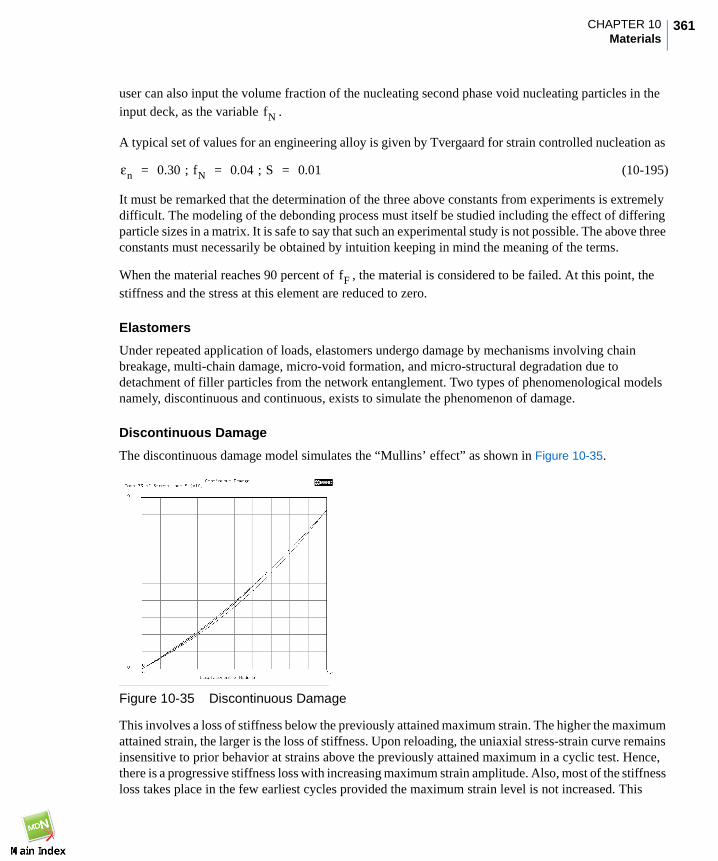
361CHAPTER 10Materials
user can also input the volume fraction of the nucleating second phase void nucleating particles in theinput deck, as the variable .
A typical set of values for an engineering alloy is given by Tvergaard for strain controlled nucleation as
(10-195)
It must be remarked that the determination of the three above constants from experiments is extremelydifficult. The modeling of the debonding process must itself be studied including the effect of differingparticle sizes in a matrix. It is safe to say that such an experimental study is not possible. The above threeconstants must necessarily be obtained by intuition keeping in mind the meaning of the terms.
When the material reaches 90 percent of , the material is considered to be failed. At this point, thestiffness and the stress at this element are reduced to zero.
Elastomers
Under repeated application of loads, elastomers undergo damage by mechanisms involving chainbreakage, multi-chain damage, micro-void formation, and micro-structural degradation due todetachment of filler particles from the network entanglement. Two types of phenomenological modelsnamely, discontinuous and continuous, exists to simulate the phenomenon of damage.
Discontinuous Damage
The discontinuous damage model simulates the “Mullins’ effect” as shown in Figure 10-35.
Figure 10-35 Discontinuous Damage
This involves a loss of stiffness below the previously attained maximum strain. The higher the maximumattained strain, the larger is the loss of stiffness. Upon reloading, the uniaxial stress-strain curve remainsinsensitive to prior behavior at strains above the previously attained maximum in a cyclic test. Hence,there is a progressive stiffness loss with increasing maximum strain amplitude. Also, most of the stiffnessloss takes place in the few earliest cycles provided the maximum strain level is not increased. This
fN
εn 0.30 ; fN 0.04 ; S 0.01= = =
fF

MSC.Nastran 2007 r1 Implicit Nonlinear (SOL 600) User’s Guide362
phenomenon is found in both filled as well as natural rubber although the higher levels of carbon blackparticles increase the hysteresis and the loss of stiffness. The free energy, W, can be written as:
(10-196)
where is the nominal strain energy function, and
(10-197)
determines the evolution of the discontinuous damage. The reduced form of Clausius-Duhem dissipationinequality yields the stress as:
(10-198)
Mathematically, the discontinuous damage model has a structure very similar to that of strain spaceplasticity. Hence, if a damage surface is defined as:
(10-199)
The loading condition for damage can be expressed in terms of the Kuhn-Tucker conditions:
(10-200)
The consistent tangent can be derived as:
(10-201)
Continuous Damage
The continuous damage model can simulate the damage accumulation for strain cycles for which thevalues of effective energy is below the maximum attained value of the past history as shown inFigure 10-36.
W K α β,( )W0
=
W0
α max W0( )=
S 2K α β,( ) ∂W0
∂C-----------=
Φ W α 0≤–=
Φ 0≤ α·
0≥ α·
Φ 0=
C 4 K∂2
W0
∂C∂C--------------- ∂K
∂W0
----------- ∂W0
∂C----------- ∂W
0
∂C-----------⊗+=

363CHAPTER 10Materials
Figure 10-36 Continuous Damage
This model can be used to simulate fatigue behavior. More realistic modeling of fatigue would require adeparture from the phenomenological approach to damage. The evolution of continuous damageparameter is governed by the arc length of the effective strain energy as:
(10-202)
Hence, β accumulates continuously within the deformation process.
The Kachanov factor is implemented in MSC.Nastran Implicit Nonlinear through both anadditive as well as a multiplicative decomposition of these two effects as:
(10-203)
(10-204)
You specify the phenomenological parameters and . If is not defined, it
is automatically determined such that, at zero values of and , the Kachanov factor . If,
according to Equation (10-203) or Equation (10-204) the value of exceeds 1, is set back to 1.
The above damage model is available for deviatoric behavior. In addition, viscoelastic behavior can beincluded. Finally, the user subroutine, UELDAM available starting in version 2005, can be used to definedamage functions different from Equation (10-211) to Equation (10-214).
β ∂∂s ′-------W
0s′( ) s ′d
0
t
∫=
K α β,( )
K α β,( ) d∞
dnα α
ηn------–
dnβ β
λn-----–
exp
n 1=
2
∑+exp
n 1=
2
∑+=
K α β,( ) d∞
dn
α δnβ+
ηn--------------------–
exp
n 1=
2
∑+=
dnα
dnβ ηn λn dn δn, , , , , d
∞d
∞
α β K 1=
K K

MSC.Nastran 2007 r1 Implicit Nonlinear (SOL 600) User’s Guide364
The parameters required for the continuous or discontinuous damage model can be obtained using theexperimental data fitting option in Mentat.
Specifying Hyperelastic Damage Model Entries
The hyperelastic damage model described above can be selected with the MATHED Bulk Data entry.
References• MATHED (SOL 600), 1565 of the MSC.Nastran Quick Reference Guide.
MSC.Patran Materials Application Input Data
MSC.Patran does not support this option in the current release.
Entry DescriptionMATHED Specifies damage model properties for hyperelastic materials to be used for
static, quasi static or transient dynamic analysis in MSC.Nastran ImplicitNonlinear (SOL 600) only.

365CHAPTER 10Materials
CreepCreep is an important factor in elevated-temperature stress analysis. In MSC.Nastran Implicit Nonlinear,creep is represented by a Maxwell model. Creep is a time-dependent, inelastic behavior, and can occurat any stress level (that is, either below or above the yield stress of a material). The creep behavior canbe characterized as primary, secondary, and tertiary creep, as shown in Figure 10-39. Engineeringanalysis is often limited to the primary and secondary creep regions. Tertiary creep in a uniaxialspecimen is usually associated with geometric instabilities, such as necking. The major differencebetween the primary and secondary creep is that the creep strain rate is much larger in the primary creepregion than it is in the secondary creep region. The creep strain rate is the slope of the creep strain-timecurve. The creep strain rate is generally dependent on stress, temperature, and time.
The creep data can be specified in either an exponent form or in a piecewise linear curve.
(10-205)
Figure 10-37 Creep Strain Versus Time (Uniaxial Test at Constant Stress and Temperature)
Forms of Creep Material Law
There are three possible modes of input for creep constitutive data.
1. Express the dependence of equivalent creep strain rate on any independent parameter through apiecewise linear relationship. The equivalent creep strain rate is then assumed to be a piecewiselinear approximation to
(10-206)
ε·
c dεc
dt--------=
Note: Primary Creep: Fast decrease in creep strain rateSecondary Creep: Slow decrease in creep strain rateTertiary Creep: Fast increase in creep strain rate
SecondaryCreep
PrimaryCreep
TertiaryCreep
Creep StrainεC
Time (t)
ε· c
A f σ( ) g εc( ) h T( ) dk t( )dt
-------------••••=

MSC.Nastran 2007 r1 Implicit Nonlinear (SOL 600) User’s Guide366
where A is a constant; is equivalent creep strain rate; and , , , and are equivalent
stress, equivalent creep strain, temperature and time, respectively. The functions , , , and
are piecewise linear. This representation is shown in Figure 10-40. (Any of the functions ( , ,
, or ) can be set to unity by setting the number of piecewise linear slopes for that relation tozero on the input data.)
2. The dependence of equivalent creep strain rate on any independent parameter can be givendirectly in power law form by the appropriate exponent. The equivalent creep strain rate is
(10-207)
This is often adequate for engineering metals at constant temperature where Norton’s rule is agood approximation.
(10-208)
3. Use the MATEP material to activate the ORNL (Oak Ridge National Laboratory rules) capabilityof the program.
Isotropic creep behavior is based on a von Mises creep potential described by the equivalentcreep law
(10-209)
Figure 10-38 Piecewise Linear Representation of Creep Data
ε· c σ ε
cT t
f g h k
f g
h k
ε· c
Aσm ε· c( )
nTp qtq 1–( )•••=
ε· c
A= σn
ε·
f σ ε· c
T t, , ,( )=
(1) Slope-Break Point Data S1X1 S2X2 S3X3(2) Function-Variable Data F1X1 F2X2 F3X3 F4X4
Function F (X)
[Such as t ,
g , h (T),
k (t)]
σ( )
εc
( )
X1
F1
X2
F2
X3
F3
X4
F4
S1
S2
S3
Variable X (Such as σ, εC, T, t)

367CHAPTER 10Materials
The material creep behavior is described by
(10-210)
During creep, the creep strain rate usually decreases. This effect is called creep hardening and can be afunction of time or creep strain. The following section discusses the difference between these two typesof hardening.
Consider a simple power law that illustrates the difference between time and strain-hardening rules forthe calculation of the creep strain rate.
(10-211)
where is the creep strain, and are values obtained from experiments and is time. The creep rate
can be obtained by taking the derivative with respect to time
(10-212)
However, being greater than 0, we can compute the time as
(10-213)
Substituting Equation (10-209) into Equation (10-212) we have
(10-214)
Equation (10-213) shows that the creep strain rate is a function of time (time hardening).Equation (10-214) indicates that the creep strain rate is dependent on the creep strain (strain hardening).The creep strain rates calculated from these two hardening rules generally are different. The selection ofa hardening rule in creep analysis must be based on data obtained from experimental results.Figure 10-41 and Figure 10-42 show time and strain hardening rules in a variable state of stress. It isassumed that the stress in a structure varies from to to ; depending upon the model chosen,
different creep strain rates are calculated accordingly at points 1, 2, 3, and 4. Obviously, creep strainrates obtained from the time hardening rule are quite different from those obtained by the strainhardening rule.
ε· c
i j ε· c ∂σ
∂σi j----------
=
εc βtn=
εc β n t
εc
ε· c dεc
dt-------- nβ tn 1–= =
t t
tεc
β-----
1 n/=
ε· c
nβtn 1– n β1 n⁄ εc( ) n 1–( ) n⁄( )( )= =
σ1 σ2 σ3

MSC.Nastran 2007 r1 Implicit Nonlinear (SOL 600) User’s Guide368
Figure 10-39 Time Hardening
Figure 10-40 Strain Hardening
Oak Ridge National Laboratory LawsOak Ridge National Laboratory (ORNL) has performed a large number of creep tests on stainless andother alloy steels. It has also set certain rules that characterize creep behavior for application in thenuclear structures. A summary of the ORNL rules on creep is discussed in MSC.Marc Volume A, Theoryand User Information. The references listed at the end of this section offer a more detailed discussion ofthe ORNL rules.
εcσ1
0
1
2
3
4
t
σ2
σ3
εcσ1
0
12
3
4
t
σ2
σ3

369CHAPTER 10Materials
Viscoplasticity (Explicit Formulation)The creep (Maxwell) model can be modified to include a plastic element (as shown in Figure 10-43).This plastic element is inactive when the stress ( ) is less than the yield stress ( ) of the material. The
modified model is an elasto-viscoplasticity model and is capable of producing some observed effects ofcreep and plasticity. In addition, the viscoplastic model can be used to generate time-independentplasticity solutions when stationary conditions are reached. At the other extreme, the viscoplastic modelcan reproduce standard creep phenomena. The model allows the treatment of nonassociated flow rulesand strain softening which present difficulties in conventional (tangent modulus) plasticity analyses.
It is recommended that you use the implicit formulation described in the following paragraphs to modelgeneral viscoplastic materials.
Figure 10-41 Uniaxial Representation of Viscoplastic Material
Creep (Implicit Formulation)This formulation, as opposed to that described in the previous section, is fully implicit. A fully implicitformulation is unconditionally stable for any choice of time step size; hence, allowing a larger time stepthan permissible using the explicit method. Additionally, this is more accurate than the explicit method.The disadvantage is that each increment may be more computationally expensive. There are two methodsfor defining the inelastic strain rate. The creep model definition option can be used to define a Maxwellcreep model. The back stress must be specified through the field reserved for the yield stress in the MAT1or other material definitions. There is no creep strain when the stress is less than the back stress. Theequivalent creep strain increment is expressed as
(10-215)
and the inelastic deviatoric strain components are
σ σy
ee
evp
σ
Plastic ElementInactive if σ < σy
εp εvp=
ε· c
Aσm
ε· c
( )n
• TP• qt
q 1–•=
∆εi ji 3
2---∆ε
iσ′i j
σ---------=

MSC.Nastran 2007 r1 Implicit Nonlinear (SOL 600) User’s Guide370
where is the deviatoric stress at the end of the increment and is the back stress. is a function
of temperature, time, etc. Creep only occurs if sigma is greater .
One of three tangent matrices may be formed. The first uses an elastic tangent, which requires moreiterations, but can be computationally efficient because re-assembly might not be required. The seconduses an algorithmic tangent that provides the best behavior for small strain power law creep. The thirduses a secant (approximate) tangent that gives the best behavior for general viscoplastic models.
Specifying Creep Material EntriesEach of the creep models described in this section can be selected with the MATVP Bulk Data entry.MATVP is the only form of creep data material input supported by SOL 600, ie.e., no other MSC.Nastrancreep data formats are supported by SOL 600.
References• MATVP (SOL 600), 1613 of the MSC.Nastran Quick Reference Guide.
MSC.Patran Materials Application Input Data
To define creep behavior in MSC.Patran:
1. From the Materials Application form, set the Action>Object>Method combination toCreate>Isotropic-or-Orthotropic-or-Anisotropic>Manual Input.
2. Click Input Properties..., and select Creep from the Constitutive Model pull-down menu andMATVP from the Creep Data Input pull-down menu.
Creep material models require the following MATVP material data via the Input Properties subform onthe Materials Application form.
Entry Description
MATVP Specifies viscoplastic or creep material properties to be used for quasi-staticanalysis in MSC.Nastran Implicit Nonlinear (SOL 600) only.
Isotropic-Anisotropic-Orthotropic Description
Coefficient Specifies the coefficient, A.
Exponent of Temperature Defines temperature exponent.
Temperature vs. Creep Strain References a material field of temperature vs. value. OverridesExponent of Temperature if present.
Exponent of Stress Defines stress exponent
Creep Strain vs. Stress References a material field of stress vs. value. OverridesExponent of Stress if present.
Exponent of Creep Strain Defines creep strain exponent.
σ′i j σy A
σ σy

371CHAPTER 10Materials
Strain Rate vs. Creep Strain References a material field of strain rate vs. value. OverridesExponent of Creep Strain if present.
Exponent of Time Defines time exponent.
Time vs. Creep Strain References a material field of time vs. value. OverridesExponent of Time if present.
Back Stress Defines the back stress for implicit creep
Isotropic-Anisotropic-Orthotropic Description

MSC.Nastran 2007 r1 Implicit Nonlinear (SOL 600) User’s Guide372
CompositeComposite materials are composed of a mixture of two or more constituents, giving them mechanical andthermal properties which can be significantly better than those of homogeneous metals, polymers andceramics.
Laminate composite materials are based on layering homogeneous materials using one of severalmethods. In order to define a laminate composite material, you must define the homogeneous materialsthat form the layers, the thickness of each layer, and the orientation angle of the layers relative to thestandard coordinate axis being used for the model. The orientation is particularly important fororthotropic and anisotropic materials, whose properties vary in different directions. The material in eachlayer may be either linear or nonlinear. Tightly bonded layers (layered materials) are often stacked in thethickness direction of beam, plate, shell structures, or solids.
Figure 10-42 identifies the locations of integration points through the thickness of beam and shellelements with and without a composite formulation.
Note that when the COMPOSITE option is used, as shown in Figure 10-42, the layer points are positionedmidway through each layer. When the COMPOSITE option is not used, the layer points are equidistantlyspaced between the top and bottom surfaces. MSC.Nastran Implicit Nonlinear performs a numericalintegration through the thickness. If the COMPOSITE option is used, the trapezoidal method isemployed; otherwise, Simpson’s rule is used.
Each layer is a “ply”, and each ply canhave a different material, thickness, ormaterial orientation (angle).

373CHAPTER 10Materials
Figure 10-42 Integration Points through the Thickness of Beam and Shell Elements
Figure 10-43 shows the location of integration points through the thickness of continuum elements.MSC.Nastran Implicit Nonlinear forms the element stiffness matrix by performing numerical integrationbased on the standard isoparametric concept.
Figure 10-43 Integration Points through the Thickness of Continuum Elements
Specifying Composite Material EntriesMSC.Nastran provides a property definition specifically for performing composite analysis. You specifythe material properties and orientation for each of the layers and MSC.Nastran produces the equivalentPSHELL and MAT2 entries for shells. This is extended to PSOLID and MATORTH for SOL 600 only.
The stacking direction for 3-D composite solids was added with a new entry, MSTACK.
Entry Description
PCOMP Defines the properties of an n-ply composite material laminate.
****
*****Beams or Shells with
Composite OptionBeams or Shells without
Composite Option
**** *
***

MSC.Nastran 2007 r1 Implicit Nonlinear (SOL 600) User’s Guide374
GasketEngine gaskets are used to seal the metal parts of the engine to prevent steam or gas from escaping. Theyare complex (often multi-layer) components, usually rather thin and typically made of several differentmaterials of varying thickness. The gaskets are carefully designed to have a specific behavior in thethickness direction. This is to ensure that the joints remain sealed when the metal parts are loaded bythermal or mechanical loads. The through-thickness behavior, usually expressed as a relation betweenthe pressure on the gasket and the closure distance of the gasket, is highly nonlinear, often involves largeplastic deformations, and is difficult to capture with a standard material model. The alternative ofmodeling the gasket in detail by taking every individual material into account in the finite element modelof the engine is not feasible. It requires a lot of elements which makes the model unacceptably large.Also, determining the material properties of the individual materials might be cumbersome.
The gasket material model addresses these problems by allowing gaskets to be modeled with only oneelement through the thickness, while the experimentally or analytically determined complexpressure-closure relationship in that direction can be used directly as input for the material model. Thematerial must be used together with 2-D or 3-D first-order solid composite element types or 2-Daxi-symmetric elements. In that case, these elements consists of one layer and have only one integrationpoint in the thickness direction of the element.
Constitutive Model
The behavior in the thickness direction, the transverse shear behavior, and the membrane behavior arefully uncoupled in the gasket material model. In subsequent sections, these three deformation modesare discussed.
Local Coordinate System
The material model is most conveniently described in terms of a local coordinate system for theintegration points of the element (see Figure 10-44). For three-dimensional elements, the first and seconddirections of the coordinate system are tangential to the midsurface of the element at the integration point.The third direction is the thickness direction of the gasket and is perpendicular to the midsurface. Fortwo-dimensional elements, the first direction of the coordinate system is the direction of the midsurfaceat the integration point, the second direction is the thickness direction of the gasket and is perpendicularto the midsurface, and the third direction coincides with the global 3-direction.
In a total Lagrange formulation, the orientation of the local coordinate system is determined in theundeformed configuration and is fixed. In an updated Lagrange formulation, the orientation isdetermined in the current configuration and is updated during the analysis.

375CHAPTER 10Materials
Figure 10-44 The Location of the Integration Points and the Local Coordinate Systems inTwo- and Three-dimensional Gasket Elements
Thickness Direction - Compression
In the thickness direction, the material exhibits the typical gasket behavior in compression, as depictedin Figure 10-45. After an initial nonlinear elastic response (section AB), the gasket starts to yield if thepressure p on the gasket exceeds the initial yield pressure py0. Upon further loading, plastic deformationincreases, accompanied by (possibly nonlinear) hardening, until the gasket is fully compressed (sectionBD). Unloading occurs in this stage along nonlinear elastic paths (section FG, for example). When thegasket is fully compressed, loading and unloading occurs along a new nonlinear elastic path (sectionCDE), while retaining the permanent deformation built up during compression. No additional plasticdeformation is developed once the gasket is fully compressed.
The loading and unloading paths of the gasket are usually established experimentally by compressing thegasket, unloading it again, and repeating this cycle a number of times for increasing pressures. Theresulting pressure-closure data can be used as input for the material model. The user must supply theloading path and may specify up to ten unloading paths. In addition, the initial yield pressure py0 mustbe given. The loading path should consist of both the elastic part of the loading path and the hardeningpart, if present. If no unloading paths are supplied or if the yield pressure is not reached by the loadingpath, the gasket is assumed to be elastic. In that case, loading and unloading occurs along theloading path.
The loading and unloading paths must be defined using the TABLES1 bulk data entries and must relatethe pressure on the gasket to the gasket closure. The unloading paths specify the elastic unloading of thegasket at different amounts of plastic deformation; the closure at zero pressure is taken as the plasticclosure on the unloading path. If unloading occurs at an amount of plastic deformation for which no pathhas been specified, the unloading path is constructed automatically by linear interpolation between thetwo nearest user supplied paths. The unloading path, supplied by the user, with the largest amount ofplastic deformation is taken as the elastic path at full compression of the gasket.
For example, in Figure 10-45, the loading path is given by the sections AB (elastic part) and BD(hardening part) and the initial yield pressure is the pressure at point B. The (single) unloading path iscurve CDE. The latter is also the elastic path at full compression of the gasket. The amount of plasticclosure on the unloading path is cp1. The dashed curve FG is the unloading path at a certain plastic
1
2
Midsurface
Integration Point
1
2
3
MidsurfaceIntegration Point

MSC.Nastran 2007 r1 Implicit Nonlinear (SOL 600) User’s Guide376
closure cp that is constructed by interpolation from the elastic part of the loading path (section AB) and
the unloading path CD.
Figure 10-45 Pressure-closure Relation of a Gasket
The compressive behavior in the thickness direction is implemented by decomposing the gasket closurerate into an elastic and a plastic part:
(10-216)
Of these two parts, only the elastic part contributes to the pressure. The constitutive equation is given bythe following rate equation:
(10-217)
Here, Dc is the consistent tangent to the pressure-closure curve.
Plastic deformation develops when the pressure p equals the current yield pressure py. The latter is afunction of the amount of plastic deformation developed so far and is given by the hardening part of theloading path (section BD in Figure 10-45).
py0
py1
py
cp0 cp1cp cy0 cy1cyA
B
C
D
E
F
G
Gasket Closure Distance c
Gas
ketP
ress
ure
p
loading path
unloading path
c·
c·e
c·p
+=
p·
Dcc·e
Dc c·
c·p
–( )= =

377CHAPTER 10Materials
Initial Gap
The thickness of a gasket can vary considerably throughout the sealing region. Since the gasket ismodeled with only one element through the thickness, this can lead to meshing difficulties at theboundaries between thick regions and thin regions. The initial gap parameter can be used to solve this.The parameter basically shifts the loading and unloading curves in the positive closure direction. As longas the closure distance of the gasket elements is smaller than the initial gap, no pressure is built up in thegasket. The sealing region can thus be modeled as a flat sheet of uniform thickness and the initial gapparameter can be set for those regions where the gasket is actually thinner than the elements of the finiteelement mesh used to model it.
Thickness Direction - Tension
The tensile behavior of the gasket in the thickness direction is linear elastic and is governed by a tensilemodulus Dt. The latter is defined as a pressure per unit closure distance (that is, length).
Transverse Shear and Membrane Behavior
The transverse shear is defined in the 2-3 and 3-1 planes of the local coordinate system (for three-dimensional elements) or the 1-2 plane (for two-dimensional elements). It is linear elastic andcharacterized by a transverse shear modulus Gt.
The membrane behavior is defined in the local 1-2 plane (for three-dimensional elements) or the local3-1 plane (for two-dimensional elements) and is linear elastic and isotropic. Young’s modulus Em and
Poisson’s ratio νm that govern the membrane behavior are taken from an existing material that must be
defined using the MAT1 bulk data entry. Multiple gasket material can refer to the same isotropic materialfor their membrane properties (see also the GASKET model definition option in MSC.Marc Volume C:Program Input).
Thermal Expansion
The thermal expansion of the gasket material is isotropic and the thermal expansion coefficient are takenfrom the isotropic material that also describes the membrane behavior.
Constitutive Equations
As mentioned above, the behavior in the thickness direction of the gasket is formulated as a relationbetween the pressure p on the gasket and the gasket closure distance c. In order to formulate theconstitutive equations of the gasket material, this relation must first be written in terms of stresses andstrains. This depends heavily on the stress and strain tensor employed in the analysis. For small strainanalyses, for example, the engineering stress and strain are used. In that case, the gasket closure rate andthe pressure rate are related to the strain rate and the stress rate by
and (10-218)
in which h is the thickness of the gasket.
c hε–= ∆p ∆σ–=

MSC.Nastran 2007 r1 Implicit Nonlinear (SOL 600) User’s Guide378
The resulting constitutive equation for three-dimensional elements, expressed in the local coordinatesystem of the integration, now reads
(10-219)
in which C = hDc. For two-dimensional elements, the equation is given by
(10-220)
For large deformations in a total Lagrange formulation, in which the Green-Lagrange strains and thesecond Piola-Kirchhoff stresses are employed (as well as in an updated Lagrange environment) inwhich the logarithmic strains and Cauchy stresses are being used, similar but more complex relationscan be derived.
Specifying Gasket Material EntriesThe MATG provides specifically for modeling gasket materials.
Entry Description
MATG Specifies gasket material properties to be used in MSC.Nastran ImplicitNonlinear (SOL 600) only.
MATTG Specifies gasket material property temperature variation to be used inMSC.Nastran Implicit Nonlinear (SOL 600) only.
σ11
σ22
σ33
σ12
σ23
σ31
Em
1 νm2
–-----------------
νmEm
1 νm2
–----------------- 0 0 0 0
νmEm
1 νm2
–-----------------
Em
1 νm2
–----------------- 0 0 0 0
0 0 C 0 0 0
0 0 0Em
2 1 νm+( )-------------------------- 0 0
0 0 0 0 Gt 0
0 0 0 0 0 Gt
ε11
ε22
ε33 ∆ε33p
–
γ12
γ23
γ31
=
σ11
σ22
σ33
σ12
Em
1 νm2
–----------------- 0
νmEm
1 νm2
–----------------- 0
0 C 0 0
νmEm
1 νm2
–----------------- 0
Em
1 νm2
–----------------- 0
0 0 0 Gt
ε11
ε22 ∆ε22p
–
ε33
γ12
=

379CHAPTER 10Materials
References• MATG (SOL 600), 1556 of the MSC.Nastran Quick Reference Guide.• MATTG (SOL 600), 1598 of the MSC.Nastran Quick Reference Guide.
MSC.Patran Materials Application Input Data
MSC.Patran 2005 support this option.

MSC.Nastran 2007 r1 Implicit Nonlinear (SOL 600) User’s Guide380
Material DampingIn direct integration analysis, the user very often defines energy dissipation mechanisms as part of thebasic model - dashpots, inelastic material behavior, etc. In such cases, there is usually no need tointroduce additional “structural” or general damping: it is unimportant compared to these otherdissipative effects. However, some models do not have such dissipation sources (an example is a linearsystem with chattering contact, such as a pipeline in a seismic event). In such cases, it is usually desirableto introduce some general low level of damping. MSC.Nastran Implicit Nonlinear provides “Rayleigh”damping for this purpose. The user includes the two Rayleigh damping factors, αR for mass proportionaldamping and βR for stiffness proportional damping on the NLSTRAT Bulk Data entry. In the case of
elements the damping values must be used in conjunction with these property references. For a linearproblem, these provide a damping matrix [C] as described above:
[C]=αR[M]+βR[K].
Since the model may have quite general nonlinear response, the concept of “stiffness proportionaldamping” must be generalized, since it is possible for the tangent stiffness matrix to have negativeeigenvalues (which would imply negative damping). To overcome this problem, βR is interpreted asdefining viscous material damping which creates an additional “damping stress,” σd, proportional to thetotal strain rate:
(10-221)
Here D0el is the material’s initial (virgin) elastic stiffness. This damping stress is added to the stress
caused by the constitutive response at the integration point when the dynamic equilibrium equations areformed, but it is not included in the stress output. This allows damping to be introduced for any nonlinearcase, and provides standard Rayleigh damping for linear cases.
Since the βR factor introduces damping proportional to the strain rate, this may be thought of as dampingassociated with the material itself, while the αR factor introduces damping forces caused by the absolutevelocities of the model, and so simulates the idea of the model moving through a viscous “ether” (apermeating, still fluid, so that any motion of any point in the model causes damping).
The αR factor is applied to all elements that have mass. The βR factor applies to all elastic elements and
to beam and shell elements. The βR factor is not applied to spring elements. Discrete dashpot elementsshould be used as needed for springs.
σd βD0elε
·=

381CHAPTER 10Materials
Specifying Material Damping EntriesParameters for material damping are input through the NLSTRAT entry.
References• NLSTRAT (SOL 600) (p. 2005) in the MSC.Nastran Quick Reference Guide.• NLDAMP (SOL 600) (p. 1987) in the MSC.Nastran Quick Reference Guide.
MSC.Patran Materials Application Input Data
MSC.Patran 2005 does not yet support material damping specified by the NLDAMP card, but you canspecify the transient analysis damping parameters on the NLSTRAT card under the Load IncrementParameters subform.
Entry DescriptionNLSTRAT Defines transient analysis damping parameters BETA, GAMMA,
GAMMA1, GAMMA2.
NLDAMP Defines damping constants for nonlinear analysis when MSC.Marc isexecuted from MSC.Nastran used in SOL 600 only (Not supported inMSC.Patran 2004).
Isotropic Description
Gamma (Newmark) Mass proportional damping coefficient.
Beta (Newmark) Stiffness proportional damping coefficient.

MSC.Nastran 2007 r1 Implicit Nonlinear (SOL 600) User’s Guide382
Experimental Data FittingThis is a very useful tool available under the Tools pull-down menu from the main MSC.Patran form andis available if the Analysis Preference is set to MSC.Nastran.
The tool is used to curve fit experimentally derived,raw elastomeric material data and fit a number ofmaterial models to the data. The data can then besaved as constitutive hyperelastic and/orviscoelastic models for use in anMSC.NastranImplicit Nonlinear or MSC.Marc analysis.
The operation of curve fitting is done in three basicsteps corresponding to the actions in the Actionpull-down menu.
1. Import the Raw Data - data is read fromstandard ASCII files and stored inMSC.Patran in the form a field (table).
2. Select the Test Data - the fields from theraw data are associated to a test type.
3. Calculate the Properties - the curve fit isdone to the selected test data; coefficientsare calculated based on the selected materialmodel; curve fit is graphically displayedand the properties can be saved as aconstitutive model for a later analysis.
Import Raw Data
Importing the data is done by following these steps:
1. Enter a New Field Name - this is the nameof the raw data table as it will be stored in MSC.Patran as a material field.
2. Select the Independent Variable - this is defaulted to Strain but could be any of Strain, Time,Frequency, Temperature, or Strain Rate.
3. Select the File and press the Apply button.
The following notes are made:
• You can skip any number of header lines in the raw data file by setting the Header Lines toSkip widget.
• You may edit the raw data file after selecting it by using the Edit File... button. The editor isNotepad on Windows platforms and vi on UNIX platforms unless you change theenvironment variable P3_EDITOR to reference a different editor. The editor must be in theuser’s path or the entire pathname must be referenced.
Experimental Data Fitting

383CHAPTER 10Materials
• Raw data files may have up to three columns of data. By default the first column of data is theindependent variable value. The second column is the measured data, and the last column canbe the area reduction or volumetric data. More than three columns is not accepted. If the thirdcolumn is blank, the material is considered incompressible.
• The data may be space, tab, or comma delimited.
• If you have cross sectional area reduction data in the third column, you can give it an optionalfield name also. If you do not specify that you have this data and a third column is detected,two fields will still be created and a _C1 and _C2 will be appended to the given field name.
• If for some reason the independent and dependent columns need to be interchanged, you canturn this toggle on. Check your imported fields before proceeding to ensure they are correct.This is done in the Fields application.
• When you press the Apply button, you will be taken to the second step. If you need to importmore than one file, you will have to reset the Action pull-down.
Experimental Data Fitting
Import Raw Data Description
New Field The field name under which the raw data will be saved. For an explanation ofwhat the raw data files should contain, see the description on each mode(Uniaxial, Biaxial, etc.) in the table for Select Test Data.
Area Data If volumetric data or cross sectional area reduction data is stored in the thirdcolumn of a raw data file it will be imported automatically and two field willbe created, one with a _C1 and the other with a _C1 appended to the name.Optionally, you can give it it’s own name by turning this toggle ON.
Area Field Name If the Area Data toggle is on, you supply the name to the field of volumetricor area data here.
IndependentVariable
This defines the independent variable. The material field created from readingthe raw data will be tagged with this independent variable. This is simply alabel and has no effect on the actual curve fits.
Header Lines toSkip
If any header lines in the data file are to be skipped before the raw data isprocessed, you can specify this with this databox.
Select File Select a raw data file. The .dat and .csv file types are filtered by default. csvfiles are comma separated and created by Microsoft Excel.
Edit File Once a file has been selected you may edit it with Notepad on Windows andvi on UNIX. The editor can be changed by setting the environment variableP3_EDITOR to the editor or choice. The editor command must be in theuser’s path or the full path must be provided as part of the P3_EDITORenvironment variable.

MSC.Nastran 2007 r1 Implicit Nonlinear (SOL 600) User’s Guide384
Select Test Data
Once the raw test data is imported, you mustassociate with a particular test type or mode byfollowing these steps:
1. Put the cursor in the data field of theappropriate type of test.
2. Select associated field from the SelectMaterial Test Data listbox which shouldhave a list of the imported raw data fields.
3. Repeat this for each test you wish to includein the calculations (curve fit).
The following notes are made:
• Typical stress-strain data forDeformation Mode tests arereferenced in the Primary column. Ifyou have volumetric data, these areentered in the Secondary columndataboxes and are optional.
• For Viscoelastic (time relaxation data),you must turn ON the ViscoElastictoggle. Only viscoelastic curve fittingwill be done in this case. To return toDeformation Mode, turn this toggleOFF.
• Damage models are not yet supported.
• When you press the Apply button, youwill be taken to the third step.
Apply This command will import the raw data and save it as a field(s) in the name(s)given in New Field (and/or Area Field Name) databoxes. You will also betaken to automatically to the Select Test Data action which is the next step.If you need to import multiple raw data files, you will have to set the Actionback to Import Raw Data.
Cancel Closes the Experimental Data Fitting tool.
Experimental Data Fitting
Import Raw Data Description

385CHAPTER 10Materials
Experimental Data Fitting
Select Test Data Description
Uniaxial
Biaxial
Planar Shear
Simple Shear
Volumetric
Select the field of raw test data corresponding to each of these tests if theyexist. You need to supply at least one. The stress-strain data field isreferenced in the Primary column. If you have volumetric or area datafields, they are referenced in the Secondary column. If no Secondary fieldis supplied, the material models are assumed incompressible.
For time independent elastomeric materials (uniaxial, biaxial, planarshear, simple shear and volumetric tests) the data should be as such in theraw data file:
eng. strain_1, eng. stress_1, volumetric data_1
eng. strain_2, eng. stress_2, volumetric data_2
. . .
eng. strain_n, eng. stress_n, volumetric data_n
If, for uniaxial, biaxial or planar shear data, the third column is left empty,the material is assumed to be incompressible.
Viscoelastic Turn this toggle ON if you wish to do a data fit on viscoelastic relaxationdata.
For visco-elastic material behavior (shear relaxation, bulk relaxation andenergy relaxation tests) the data should be as such in the raw data file:
time_1, value_1 (shear modulus, bulk modulus or strain energy)
time_2, value_2 (shear modulus, bulk modulus or strain energy)
. . .
time_n, value_n (shear modulus, bulk modulus or strain energy)

MSC.Nastran 2007 r1 Implicit Nonlinear (SOL 600) User’s Guide386
Damage Not yet supported. Turn this toggle ON if you wish to do a data fit ondamage models. For continuous damage (resulting from a constant strainamplitude test) the data in the raw input file should be:
cycle_1, str_energy_d_1
cycle_2, str_energy_d_2
. .
cycle_n, str_energy_d_n
In addition, before fitting the data, the free energy (which is the strainenergy density corresponding to the undamaged state) is required. Noticethat the data points should not include the range of cycles at whichdamage did not start to evaluate.
For discontinuous damage (resulting from an increasing strain amplitudetest):
str_energy_d_1, strain_energy_d_1/str_energy_d_1_undamaged
str_energy_d_2, strain_energy_d_2/str_energy_d_2_undamaged
. . .
str_energy_d_n, strain_energy_d_n/str_energy_d_n_undamaged
Notice that the data points should not include the range of cycles at whichdamage did not start to evaluate.
Viscoelastic/Damage In this field, select the Viscoelastic or Damage raw test data field.
Select Material TestData
From this listbox you select the field corresponding to the DeformationMode or the Viscoelastic/Damage data.
Apply Once the test data is associated to the respective modes, the Apply buttonwill take you to the Calculate Properties action.
Cancel Closes the Experimental Data Fitting tool.
Experimental Data Fitting
Select Test Data Description

387CHAPTER 10Materials
Calculate Properties
Once test data has been associated to a testtype or mode, the curve fit is done by followingthese steps:
1. Select the material Model you wish to doa curve fit for. The available models willdepend on the test data selected in theprevious step. Hyperelastic models willbe available for deformation mode testdata. Viscoelastic models will beavailable for relaxation test data.
2. In general you will leave Use Test Datato All for hyperelastic models. Ifhowever you only want the curve fit touse one of the deformation modes, youmay set it here.
3. Press the Compute button. Thecoefficient values will be displayed in theCoefficients spreadsheet.
4. To visually see the curve fit, press thePlot button.
You may repeat the above four steps foras many material models as you wish tocurve fit.
5. Select an existing material or type in aNew Material Name and press theApply button to save the material modelas either a Hyperelastic or Viscoelasticconstitutive model for use in asubsequent analysis.
The following notes are made:
• The plots are appended to the existingXY Window until you press theUnpost Plot button. You can turn theAppend function ON/OFF under thePlot Parameters... form.
• By default, all the deformation modesare plotted along with the raw dataeven if raw data has not beensupplied for those mode. This is very
Experimental Data Fitting

MSC.Nastran 2007 r1 Implicit Nonlinear (SOL 600) User’s Guide388
important. These additional modes are predicted for you. You should always know yourmodel’s response to each mode of deformation due to the different types of stress states. Forexample, a rule of thumb for natural rubber and some other elastomers is that the tensiletension biaxial response should be about 1.5 to 2.5 times the uniaxial tension response.
• You can turn ON/OFF these additional modes or any of the curves under the PlotParameters button as well as change the appearance of plot. More control and formatting ofthe plot can be done under the XY Plot application on the MSC.Patran application switch onthe main form.
• Viscoelastic constitutive models are useless without a Hyperelastic constitutive modelalso. Be sure your model has both defined under the same material name if you useviscoelastic properties.
• You may actually change the coefficient values in the Coefficients spread sheet if you wishto see the effect they have on the curve fit. Select one of the cells with the coefficient you wishto change, then type in a new coefficient value in the Coefficient Value data box and pressthe Return or Enter key. Then press the Plot button again. If you press the Apply button, thenew values will be saved in the supplied material name.
• For viscoelastic relaxation data, the Number of Terms used in the data fit should, as a rule ofthumb, be as many as there are decades of data.
• A number of optional parameters are available to message the data and control the curvefitting. See the table below for more detailed descriptions.

389CHAPTER 10Materials
The following tables more fully describes each widget in the Experimental Data Fitting tool:
Calculate Properties Description
Model:Neo-Hookean* This command is used if experimental data must be fitted using the Neo-Hookean strain energy function W, which is given by:
W = C10*(I1 - 3)
where I1 is the first invariant of the right Cauchy-Green strain tensor andC10 is the material parameter to be determined. For this model, avolumetric test can not be supplied. The user may enter a bulk modulus.If no bulk modulus is given, nearly incompressible material behavioris assumed.
Model:Mooney(2)* This command is used if experimental data must be fitted using the twoterm Mooney-Rivlin strain energy function W, which is given by:
W = C10*(I1 - 3) + C01*(I2 - 3)
where I1 and I2 are the first and second invariant of the right Cauchy-Green strain tensor and C10 and C01 are the material parameters to bedetermined. For this model, a volumetric test can not be supplied. The usermay enter a bulk modulus. If no bulk modulus is given, nearlyincompressible material behavior is assumed.
Model:Mooney(3)* This command is used if experimental data must be fitted using the threeterm Mooney-Rivlin strain energy function W, which is given by:
W = C10*(I1 - 3) + C01*(I2 - 3) + C11*(I1 - 3)*(I2 - 3)
where I1 and I2 are the first and second invariant of the right Cauchy-Green strain tensor and C10, C01 and C11 are the material parameters tobe determined. For this model, a volumetric test can not be supplied. Theuser may enter a bulk modulus. If no bulk modulus is given nearlyincompressible material behavior is assumed.
Model:Signiorini* This command is used if experimental data must be fitted using theSigniorini strain energy function W, which is given by:
W = C10*(I1 - 3) + C01*(I2 - 3) + C20*(I1 - 3)^2
where I1 and I2 are the first and second invariant of the right Cauchy-Green strain tensor and C10, C01 and C20 are the material parameters tobe determined. For this model, a volumetric test can not be supplied. Theuser may enter a bulk modulus. If no bulk modulus is given, nearlyincompressible material behavior is assumed.

MSC.Nastran 2007 r1 Implicit Nonlinear (SOL 600) User’s Guide390
Model:2nd OrderInvariant*
This command is used if experimental data must be fitted using the secondorder invariant strain energy function W, which is given by:
W = C10*(I1 - 3) + C01*(I2 - 3) + C11*(I1 - 3)*(I2-3) +C20*(I1 - 3)^2
where I1 and I2 are the first and second invariant of the right Cauchy-Green strain tensor and C10, C01, C11 and C20 are the material parametersto be determined. For this model, a volumetric test can not be supplied. Theuser may enter a bulk modulus. If no bulk modulus is given, nearlyincompressible material behavior is assumed.
Model:3rd OrderDeform*
This command is used if experimental data must be fitted using the thirdorder deformation strain energy function W, which is given by:
W = C10*(I1 - 3) + C01*(I2 - 3)+ C11*(I1 - 3)*(I2 - 3) +C20*(I1 - 3)^2 + C30*(I1 - 3)^3
where I1 and I2 are the first and second invariant of the right Cauchy-Green strain tensor and C10, C01, C11, C20 and C30 are the materialparameters to be determined. For this model, a volumetric test can not besupplied. The user may enter a bulk modulus. If no bulk modulus is given,nearly incompressible material behavior is assumed.
Note: The data input for all of these options has been consolidated under the Jamus-Green-Simpson option of the MSC.Patran Materials-Input-Data-Hyperelastic form.
Model:Yeoh This command is used if experimental data must be fitted using the Yeohstrain energy function W, which is given by:
W = C10*(I1 - 3) + C20*(I1 - 3)^2 + C30*(I1 - 3)^3
where I1 is the first invariant of the right Cauchy-Green strain tensor andC10, C20 and C30 are the material parameters to be determined. For thismodel, a volumetric test can not be supplied. The user may enter a bulkmodulus. If no bulk modulus is given, nearly incompressible materialbehavior is assumed.
Calculate Properties Description

391CHAPTER 10Materials
Model:Ogden This command is used if experimental data must be fitted using the Ogdenstrain energy function W, which is given by:
where lam1, lam2 and lam3 are the principal stretch ratios, J is thedeterminant of the deformation gradient, N is the number of terms andmu_n, alpha_n and K are the material parameters to be determined. Themaximum number of terms is 10, but it is recommended to use no moreterms than necessary to get a sufficiently good fit. This model can be usedfor incompressible as well as for slightly compressible elastic materials.Compressibility is included based on a constant bulk modulus. In case ofcompressibility, volumetric information is needed, preferably using avolumetric test, but volumetric data can also be included for uniaxial,biaxial and planar shear tests. In order to perform a plausible extrapolationfor the compressible Ogden model, dilatational information is neededbeyond the data set. This is achieved using linear extrapolation based onthe two start and/or end points of the measured data. This linearextrapolation may restrict the validity of the response outside the range ofthe measured data. For dual mode plotting (except for simple shear),dilatational information is needed for the compressible Ogden model. Fora volumetric test, this readily follows from the strain, but for uniaxial,biaxial and planar shear tests this must be calculated. This calculation isbased on the requirement that the stress in perpendicular direction must bezero. If the fitted coefficients do not fulfil this requirement, zero stressesare returned for such a dual mode.
Note: Ogden hyperelastic coefficients are different in MSC.Marc andMSC.Nastran. For information on experimental data fitting forthe MSC.Nastran MATHP and MATHE entries, seeExperimental Data Fitting, 301.
Calculate Properties Description
{(mu_n/alpha_n) * (J^(-alpha_n/3)) *(lam1^alpha_n + lam2^alpha_n + lam2^alpha_n- 3)} + 4.5 * K * (J^(1/3) - 1)^2
W
N
Σn 1=
=

MSC.Nastran 2007 r1 Implicit Nonlinear (SOL 600) User’s Guide392
Model:Foam This command is used if experimental data must be fitted using the foamstrain energy function W, which is given by:
where lam1, lam2 and lam3 are the principal stretch ratios, J is thedeterminant of the deformation gradient, N is the number of terms andmu_n, alpha_n and beta_n are the material parameters to be determined.The maximum number of terms is 10, but it is recommended to use nomore terms than necessary to get a sufficiently good fit. This model shouldbe used for highly compressible elastic materials. Except for the simpleshear test, volumetric information must be available. In order to perform aplausible extrapolation for the foam model, dilatational information isneeded beyond the data set. This is achieved using linear extrapolationbased on the two start and/or end points of the measured data. This linearextrapolation may restrict the validity of the response outside the range ofthe measured data. For dual mode plotting (except for simple shear),dilatational information is needed for the foam model. For a volumetrictest, this readily follows from the strain, but for uniaxial, biaxial and planarshear tests this must be calculated. This calculation is based on therequirement that the stress in perpendicular direction must be zero. If thefitted coefficients do not fulfil this requirement, zero stresses are returnedfor such a dual mode.
Calculate Properties Description
{(mu_n/alpha_n)*(lam1^alpha_n +lam2^alpha_n + lam2^alpha_n - 3)+(mu_n/beta_n)*(1 - J^beta_n)}
W
N
Σn 1=
=

393CHAPTER 10Materials
Model:Arruda-Boyce Elastomer Free Energy Function; Number of coefficients 1
Ref: "A Three-Dimensional Constitutive Model For the Large StretchBehavior of Rubber Elastic Materials"
by: Ellen M. Arruda and Mary C. Boyce
J.Mech.Phys.Solids Vol.41, No.2, pp.389-412
Parameter: N -- The number of mers in a typical polymer chain - Specifiedby the user.
Coefficient: n,k,T -- Determined by the fitter
n : Number of Polymer chains per unit volume
k : Boltzmann constant
T : Temperature
For this model, the calculation of the Bulk Modulus is not required. Avolumetric test need not be supplied.
Calculate Properties Description

MSC.Nastran 2007 r1 Implicit Nonlinear (SOL 600) User’s Guide394
Model:Gent Elastomer Free Energy Function; Number of coefficients 2
Ref: "A new constitutive relation for rubber"
by: A.N. Gent
Rubber Chemistry and Technology,
Vol.79, pp.59-61, 1996
Coefficient: E, I_m -- Determined by the fitter
E : small strain tensile modulus
I_m : maximum value for the first
invariant of deformation (I1)
WARNING: This phenomenological model is designed to exhibit finiteextensibility of polymer chains and forces the stresses and tangent toassymptote to infinity as I1 approaches Im. It is conceivable that during thesolution stage, a set of trial displacements is evaluated such that I1 > Im.In which case, the convergence ratios can be expected to oscillate, or evenworse, the solution may not converge at all. Therefor, if Im < 4, it isrecommended that loads be applied in very small increments.
For this model, the calculation of the Bulk Modulus is not required and avolumetric test need not be supplied.
Calculate Properties Description

395CHAPTER 10Materials
Model:ViscoShear Relax
This command is used if experimental shear relaxation data must be fittedusing the following Prony series expansion for the shear modulus G:
where t is the time, N is the number of terms and G_infinity, G_n and tau_nare material parameters to be determined. The data points provided by theuser must give the value of the shear modulus at different time stations,which do not need to be equi-spaced.
Model:ViscoBulk Relax
This command is used if experimental bulk relaxation data must be fittedusing the following Prony series expansion for the bulk modulus K:
where t is the time, N is the number of terms and K_infinity, K_n and tau_nare material parameters to be determined. The data points provided by theuser must give the value of the bulk modulus at different time stations,which do not need to be equi-spaced.
Model:Visco EnergyRelax
This command is used if experimental strain energy relaxation data mustbe fitted using the following Prony series expansion for the strain energy W
:
where t is the time, N is the number of terms, W0 is the instantaneous strainenergy and W_infinity, delta_n and tau_n are material parameters to bedetermined. The data points provided by the user must give the value of thestrain energy at different time stations, which do not need to be equi-spaced.
Model:Cont. Damage Not yet supported.
Model:Disc. Damage Not yet supported.
Calculate Properties Description
G(t) = G_infinity {G_n*exp(-t/tau_n)}W
N
Σn 1=
=
K(t) = K_infinity {K_n*exp(-t/tau_n)}
N
Σn 1=
K(t) = K_infinity {delta_n*W0*exp(-t/tau_n)}
N
Σn 1=

MSC.Nastran 2007 r1 Implicit Nonlinear (SOL 600) User’s Guide396
Compute This command starts the data fitting program with the selected data. Afterfitting, the measured and fitted curves can be displayed and thecorresponding material model coefficients and the least squares error arereported. For the Mooney-Rivlin, Ogden, Foam, Arruda-Boyce and Gentmodels, the response in the modes for which no data is measured, ispredicted. Notice that if volumetric data is relevant in order to predict auniaxial, biaxial or planar shear mode, this is calculated using theconstraint of a zero stress component in a direction perpendicular to thedirection of the measured stress component. If this calculation fails, thepredicted mode will contain zero stresses.
If the data set contains a large number of entries, or if the model is highlynon-linear and/or contains many coefficients, then the fitting proceduremay take some time.
Since the curve fitting procedure does not use weighting factors per datapoint, it might be useful to have many data points near regions where anaccurate response is desired.
Coefficient Value This option allows the user to manually enter the coefficients of thematerial model and updates the response curves. You must select thecoefficient to be modified from the spread sheet and then enter the valueby pressing the Return or Enter key after putting in the new coefficient.Notice that, although no fit is performed, at least one set of test data mustbe selected. This feature is available for the Mooney-Rivlin, Ogden, Foam,Arruda-Boyce and Gent material models.
Plot This plots the current curve fit. The raw data and the calculated curvefits for the supplied experimental data and the other predicted modesare plotted.
Unpost Plot This clears the plot of all curves. By default additional data fit curves areappended the XY Window.
New Material Name If a new name is supplied here and this material name does not yet exist, itwill be created with the appropriate constitutive models when the Applybutton is pressed.
Select Material If you want the hyperelastic or viscoelastic data to be saved into an existingmaterial set, select it from this listbox.
Apply This command copies the computed material model coefficients into amaterial model: it either creates a new one as indicated by the NewMaterial Name or changes an existing one as selected from SelectMaterial.
Cancel Closes the Experimental Data Fitting tool.
Calculate Properties Description

397CHAPTER 10Materials
Experimental Data Fitting
Optional Parameters Description
Uniaxial Test: A/Ao V/Vo Volumetric data of a uniaxial test can be given as: the ratio of the currentcross sectional area and the original cross sectional area (A/A0) or: theratio of the current volume and the original volume (V/V0). By default,the volumetric data is expected to be in terms of A/A0. If the actual datais in terms of V/V0, use this switch to change the type of input. Not allmaterial models need this information and therefore these widgets mayappear dimmed.
Biaxial Test: t/to V/Vo Volumetric data of an equibiaxial test can be given as: the ratio of thecurrent thickness and the original thickness (t/t0) or: the ratio of thecurrent volume and the original volume (V/V0). By default, thevolumetric data is expected to be in terms of t/t0. If the actual data is interms of V/V0, use this switch to change the type of input. Not allmaterial models need this information and therefore these widgets mayappear dimmed.
Planar Shear t/to V/Vo Volumetric data of a planar shear test can be given as: the ratio of thecurrent thickness and the original thickness (t/t0) or: the ratio of thecurrent volume and the original volume (V/V0) If the actual data is interms of V/V0, use this switch to change the type of input. Not allmaterial models need this information and therefore these widgets mayappear dimmed.
Mathematical Checks This command activates mathematical checks for Ogden and Foammaterials and causes the data fitter to discard the coefficients when oneof the mathematical conditions on them is not satisfied. These conditionsare considered to be very strict and at times no set of coefficients may befound, or the fit may be very poor.
Positive Coefficients Since curve fitting is a mathematical operation, the fitted material modelcoefficients may be physically non-realistic. This command forces thefitting procedure to return coefficients which are all positive. The qualityof the fit may be worse than that without this restriction. For exampleOgden coefficients come in pairs. If each pair of modulus and exponenthave the same sign, stability is guaranteed. If one is positive and the othernegative, the material might be unstable. Thus you must visuallydetermine the stability range of the model.

MSC.Nastran 2007 r1 Implicit Nonlinear (SOL 600) User’s Guide398
Extrapolate For Mooney-Rivlin, Ogden, Foam, Arruda-Boyce and Gent models, thiscommand gives the possibility to get the response of the material outsidethe range of measurements. This might be important if the deformationsof the structure to be analyzed exceed those of the experiments. Oneneeds to set the new left and right bounds up to which the extrapolationwill be performed. Notice that when volumetric information is provided,outside the range of measurements the volumetric data is calculatedbased on linear extrapolation using the two closest measured data points.
Error The least squares error to be minimized during data fitting can be basedon absolute or relative errors:
Err_Abs = sum {[data_measured(i) -data_calculated(i)]^2}
iErr_Rel = sum {[1 -data_calculated(i)/data_measured(i)]^2}
i
This command can be used to switch between relative (default) andabsolute errors.
Error Limit During curve fitting, an optimal set of material coefficients is searchedfor using the Downhill Simplex method. If the least squares errorcorresponding to a set of material coefficients is larger than the errorlimit, a new minimum will be searched for, unless the maximum numberof iterations has been reached. This command sets the error limit. If,upon fitting, the reported error is larger than the error limit, searching fora new minimum has been terminated due to reaching the maximumnumber of iterations.
Number of Iterations At times, the data fitter may arrive at coefficients which correspond to aminimum in the objective function, not fulfilling the least squares errorlimit. This command defines how many attempts the program will maketo exit the minimum. The maximum number of iterations is 500.
Convergence Tolerance The data fitter uses the Downhill Simplex method to find a (local)minimum. This method uses several sets of material coefficients andcalculates the corresponding objective functions. Based on the values ofthe objective functions, the sets of material coefficients are modified.This process is terminated when:
2*abs{(fh-fl)/(abs(fh)+abs(fl))} < convergencetolerance
in which fh is the highest and fl is the lowest objective functionfound so far. The process is also terminated after 2000 trials if theconvergence tolerance has not been reached. This command sets theconvergence tolerance.
Experimental Data Fitting
Optional Parameters Description

399CHAPTER 10Materials
Use Fictive Coefficient For Foam models, toggle this value to ON in order to use the fictivePoisson's ratio to create volumetric information.
Fictive Coefficient Supply the fictive Poisson’s ratio here.
OK Closes the Optional Parameters form.
Experimental Data Fitting
Plot Parameters Description
Append Curves If this toggle is ON, curves keep accumulating on the XY Window. If itis OFF, the curves are cleared each time a new data fit is done and plotted.
X-Axis OptionsY-Axis Options
You can plot the curves in linear or log scales.
Deformation Modes If any of these toggles is OFF, that particular deformation mode will beremoved from the XY Window.
OK Closes the Plot Parameters form.
Experimental Data Fitting
Optional Parameters Description
Note: The plotting and deleting of plots in this utility tool is fairly self contained and little, if any,need to use the XY Plot application is necessary. If however, you find it necessary to usethe XY Plot application and post/unpost curves, the naming convention is as such:

MSC.Nastran 2007 r1 Implicit Nonlinear (SOL 600) User’s Guide400
Raw Data Curve Name = R_"mode type"_"field id"_"color"_"marker type
Data Fit Curve Name = "model"_"mode type"_"field id"_"color"_"line type
where:
mode type (string) = "U" : Uniaxial"B" : Biaxial"P" : Planar Shear"S" : Simple Shear"V" : Volumetric"C" : VisCoelastic
model (string)= "N" : Neo-Hookean"M2" : Mooney 2"M3" : Mooney 3"S" : Signiorini"2O" : Second Order Invariant"3O" : Third Order Deformation"Y" : Yeoh"O#" : Ogden # where # is the number of terms, e.g., O2"F#" : Foam # where # is the number of terms, e.g., F3"B" : Boyce"G" : Gent"CD" : Continuous damage"DD" : Discontinuous Damange"SV" : Shear Relaxation Visco"BV" : Bulk Relaxation Visco"EV" : Energy Relaxation Visco

MSC.Nastran 2005 r3 Implicit Nonlinear (SOL 600) User’s GuideCh. 11: Element Library
11 Element Library
Overview 402
Element Selection 404
Global Element Controls 406
Mass Elements, Springs, Dampers, and Bush Elements 407
Gap Elements 409
Line Elements 410
Membranes, Panels, and Shells 411
Solid Elements 413
Beam/Bar and Shell Offsets 417
MSC.Nastran 2007 r1 Implicit Nonlinear (SOL 600) User’s Guide402
OverviewThe heart of a finite element program lies in its element library which allows you to model a structure foranalysis. MSC.Nastran has a very comprehensive element library which lets you model 1-D, 2-D, or 3-Dstructures. This section gives some basic definitions of the element types available in MSC.NastranImplicit Nonlinear. Please note, these elements differ from those used in other portions of MSC.Nastran.
Element TypesEach element has five definitive characteristics that determine its behavior:
• Class• Number of Nodes• Interpolation• Degrees of Freedom• Integration Method
Class
The type of geometric domain that an element represents determines the class of the element. Listedbelow are the classes of elements in the MSC.Nastran Implicit Nonlinear element library.
• Beam Elements - is a 3-D bar with axial, bending, and torsional stiffness.
• Shell Elements - is a curved, thin or thick structure with membrane/bending capabilities.
• Plate Elements - is a flat thin structure carrying in-plane and out-of-plane loads.
• Continuum Elements
• Plane stress is a thin plate with in-plane stresses only. All normal and shear stresses associatedwith the out-of-plane direction are assumed to be zero. (All plane strain elements lie in theglobal x-y plane.)
• Generalized plane strain is the same as plane strain except that the normal z-strain can be aprescribed constant or function of x and y.
• Axisymmetric elements are describe in 2D, but represent a full 3D structure where thegeometry and loading are both axisymmetric.
• 3D solid is a solid structure with only translational degrees of freedom for each node (linearor quadratic interpolation functions).
• Truss Elements- is a 3D rod with axial stiffness only (no bending).
• Membrane Elements -is a thin sheet with in-plane stiffness only (no bending resistance).
• Gap Elements
• Points/Springs/Damper Elements
• Rigid Constraints

403CHAPTER 11Element Library
Number of Nodes
The number of nodes for an element define where the displacements are calculated in the analysis.Elements with only corner nodes are classified as first order elements and the calculation ofdisplacements at locations within the element are made by linear interpolation. Elements thatcontain midside nodes are second order elements and quadratic interpolations are made forcalculating displacements.
In MSC.Nastran the number of nodes is designated at the end of the element name. For example, aCQUAD4 has 4 nodes.
Interpolation
Interpolation (shape) function is an assumed function relating the displacements at a point inside anelement to the displacements at the nodes of an element. In MSC.Nastran, three types of shape functionsare used: linear, quadratic, and cubic. Certain types of enhancements, such as Assumed Strain, shapefunctions, may increase the elements ability to capture accurately certain types of deformation states.
Degrees of Freedom
Degrees of freedom is the number of unknowns at a node. In the general case, there are six degrees offreedom at a node in structural analysis (three translations, three rotations). In special cases, the numberof degrees of freedom is two (translations) for plane stress, plane strain, and axisymmetric elements;three (translations) for 3-D truss element; six (three translations, three rotations) for a 3-D beamelement).
Integration
Numerical integration is a method used for evaluating integrals over an element. Element quantities –such as stresses, strains, and temperatures – are calculated at each integration point of the element. Fullintegration (quadrature) requires, for every element, 2d integration points for linear interpolation and 3dpoints for quadratic interpolation, where scalar “d” is the number of geometric dimensions of an element(that is, d = 2 for a quad; d = 3 for a hexahedron). Reduced integration uses a lower number of integrationpoints than necessary to integrate exactly. For example, for an 8-node quadrilateral, the number ofintegration points is reduced from 9 to 4 and, for a 20-node hexahedron, from 27 to 8. For some elements,an “hourglass” control method is used to insure an accurate solution.

MSC.Nastran 2007 r1 Implicit Nonlinear (SOL 600) User’s Guide404
Element SelectionThe MSC.Nastran Implicit Nonlinear element library provides a complete finite element modelingcapability. Selecting elements to use for a SOL 600 analysis can be very different than elements youmight use for other solution sequences. In particular, the large strains encountered in nonlinear analysishave implications for the element formulations.
SOL 600 selects appropriate element formulations based on the analysis type, the elements you use inconstructing your model, element properties, and global parameters. While most of the elementformulation decisions made by SOL 600 require no additional user input, some of the formulationprinciples are discussed in this section. Certain analyses may require element types other than the defaultwhich can be specified using
Element InterpolationAll of the elements in MSC.Nastran Implicit Nonlinear are formulated in “element” coordinate systemsdescribed in the MSC.Marc Volume B: Element Library. For almost all elements, primary vectorquantities (such as displacements) are defined in terms of nodal values with scalar interpolationfunctions. When the interpolation function for these vector quantities are the same interpolation functionsused to define the geometry (i.e., the position vector) the elements are called isoparametric. Suchelements are guaranteed to be able to exactly represent all rigid body modes and homogeneousdeformation modes, a necessary condition for convergence to the exact solution as the mesh is refined(i.e. the patch test).
Element IntegrationAll elements are integrated numerically. MSC.Nastran Implicit Nonlinear normally uses “full”integration elements but “reduced” integration elements are also available. For full integration, thenumber of integration points is sufficient to integrate the governing virtual work expression exactly, atleast for linear material behavior. All triangular and tetrahedral elements in MSC.Nastran ImplicitNonlinear use full integration. Reduced integration can be used for quadrilaterals and hexahedralelements; in this procedure, the number of integration points is sufficient to exactly integrate thecontributions of the strain field that are one order less then the order of the interpolation. The(incomplete) higher-order contributions to the strain field present in these elements will not be integrated.
Hourglassing
The advantage of the reduced integration elements is that the strains and stresses are calculated at thelocation that provide optimal accuracy, the so-called Barlow points. The reduced integration elementsalso tend to underestimate the stiffness of the element which often gives better results in a typicallyoverly-stiff finite element analysis displacement method. An additional advantage is that the reducednumber of integration points decreases CPU time and storage requirements. The disadvantage is that thereduced integration procedure may admit deformation modes that cause no straining at the integrationpoints. These zero-energy modes cause a phenomenon called “hourglassing,” where the zero energymode starts propagating through the mesh, leading to inaccurate solutions. This problem is particularly

405CHAPTER 11Element Library
severe in first-order quadrilaterals and hexahedrals. To prevent these excessive deformations, anadditional artificial stiffness is added to these elements. In this so-called hourglass control procedure, asmall artificial stiffness is associated with the zero-energy modes. This procedure is used in many of thealternate solid and shell elements in MSC.Nastran Implicit Nonlinear All primary elements translatedfrom the standard MSC.Nastran finite elements are fully integrated. Reduced integration elements maybe selected using PARAM,MRALIAS. For more information, see MRALIAS ID (MALIAS02, MALIAS03,etc.) (p. 732) in the ..
Figure 11-1 Hourglassing
Incompressible ElementsSometimes fully integrated solid elements are unsuitable for the analysis of (approximately)incompressible material behavior. The reason for this is that the material behavior forces the material todeform (approximately) without volume changes. Fully integrated solid element meshes, and inparticular lower-order element meshes, do not allow such deformations (other than purely homogeneousdeformation). For fully incompressible behavior, another complication occurs: the bulk modulus andhence the stiffness matrix becomes infinitely large. For this case, a mixed (Herrmann) formulation isrequired, where the displacement field is augmented with a hydrostatic pressure field. In thisformulation, only the inverse of the bulk modulus appears, and consequently the contribution of theoperator matrix vanishes. In this formulation, the hydrostatic pressure field play the role of a Lagrangemultiplier enforcing the incompressibility constraints.
Overriding MSC.Nastran Element SelectionsIn most cases MSC.Nastran selects an equivalent MSC.Marc element to use in the analysis. The selectionis based on the large number of analysis correlations between SOL 600 and SOL 100, SOL 106, or 129results. In some cases an experienced MSC.Marc user may want to use alternate elements and may doso by adding a Parameter to the MSC.nastran Input File as follows.
PARAM,MRALIAS
For more information on the MSC.Marc override parameter, see MRALIAS ID (MALIAS02, MALIAS03,etc.) (p. 732) in the .

MSC.Nastran 2007 r1 Implicit Nonlinear (SOL 600) User’s Guide406
Global Element Controls
Assumed StrainConventional isoparametric four-node plane stress and plane strain, and eight-node brick elementsbehave poorly in bending. The reason is that these elements do not capture a linear variation in shearstrain which is present in bending when a single element is used in the bending direction. As a default inMSC.Nastran Implicit Nonlinear, the element interpolation functions have been modified such that shearstrain variation can be better represented. For elastic isotropic bending problems, this allows the exactdisplacements to be obtained with only a single element through the thickness. Use PARAM,MARCASUM, 1 to activated this option.
Constant DilatationWhen performing nearly incompressible analysis with displacement based elements, the conventionalisoparametric interpolation methods result in poor behavior for lower order elements. To address thiscase, an integration scheme option is included (default) which makes the dilatational strain constantthroughout the element. Constant dilatational element formulation is preferred in approximatelyincompressible, inelastic analysis, such as large strain plasticity, because conventional elements canproduce volumetric locking due to overconstraints for nearly incompressible behavior. This option is alsothe formulation of choice for elastic-plastic analysis and creep analysis because of the potentially nearlyincompressible behavior. Use PARAM, MARCDILT, 1 to activate this option.
Setting Global Element Parameters in MSC.PatranAssumed strain, constant dilatation, plane stress, and reduced integration options, are turned ON and OFFfor the entire model.
1. On the Analysis Application form, select Solution Type..., then click Solution Parameters...
2. Use the check boxes to turn OFF and ON Assumed Strain and Constant Dilatation.

407CHAPTER 11Element Library
Mass Elements, Springs, Dampers, andBush ElementsThe following 0-D and 1-D special purpose elements allow you to model very specific types of behavior.
PBUSHT support has been added for nonlinear springs. TABLED1 can be used to specify the load-deflection curve. The PBUSHT/TBLED1 data is mapped to MSC.Marc’s SPRINGS option with table-driven force-deflection curves.
Bolt elements were added to support MSC.Marc both outside the USA and within the USA.MSC.Nastran Bulk Data entries, MBOLT and MBOLTUS reflect these new additions.
MSC.Patran FE Application Input DataThese elements are generated in MSC.Patran using the following Object/Type combination on theElement Properties Application form.
Entry Description Cross-Ref to Element Info in QRG
CMASSi Defines scalar mass elements. CMASS1, 1171
CONM1,CONM2
Defines a concentrated mass at a grid point. CONM1, 1180
CONM2, 1181
CELAS1 Defines a scalar spring element. CELAS1, 1126
CDAMPi Defines a scalar damper element. CDAMP1, 1116
CVISC Defines a viscous damper element. CVISC, 1288
CBUSH Defines a generalized spring-and-damperstructural element that may be nonlinear orfrequency dependent.*
CBUSH, 1103
CBUSH1D Defines the connectivity of aone-dimensional spring and viscousdamper element.*
CBUSH1D, 1107
*The bush element features are implemented only partially in SOL 600. Certain features such ascoordinate system ID location of the damper etc., are not available until the 2006 release. Use of thesefeatures will cause the job to terminate with a “SEVERE WARNING”. If your model does not needfields 6-9 of CBUSH or the continuation entry, you can allow the job to run by entering bulk dataPARAM, MARCBUSH,1.
Object Type Options Bulk Data Entries
0D Mass Coupled, Grounded, Lumped CONM1, CONM2
1D Mass CMASSi
0D Grounded Spring CELAS1

MSC.Nastran 2007 r1 Implicit Nonlinear (SOL 600) User’s Guide408
1D Spring CELAS1
0D Grounded Damper
1D Damper Scalar, Viscous CDAMPi, CVISC
OD Grounded Bush CBUSH
1D Bush CBUSH1D
Object Type Options Bulk Data Entries

409CHAPTER 11Element Library
Gap ElementsGap elements are an obsolete method to model contact problems. These elements allow for gap openingand closing as well as friction along a surface. Gap elements should normally be replaced with 2D or 3Dcontact. Gaps for SOL 600 are only offered for compatibility with other MSC.Nastran solutionsequences and cannot be simulated exactly the same in SOL 600 as in the other solution sequences. Thereuse is not recommended.
MSC.Patran FE Application Input DataThese elements are generated in MSC.Patran using the following Object/Type combination on theElement Properties Application form.
Entry Description Cross-Ref to Element Info in QRG
CGAP Defines a gap or friction element. CGAP, 1141
Object Type Options Bulk Data Entries
1D Gap Adaptive, Nonadaptive CGAP

MSC.Nastran 2007 r1 Implicit Nonlinear (SOL 600) User’s Guide410
Line ElementsMSC.Nastran offers a wide variety of line elements that include beams, bars, rods. Beams can be definedusing standard cross sections supplied in a library or general cross sections that are user defined.
MSC.Patran FE Application Input DataLine elements are generated in MSC.Patran using the following Object/Type combination on the ElementProperties Application form.
Entry Description Cross-Ref to Element Info in QRG
CBAR Defines a simple beam element. CBAR, 1084
CBEAM Defines a beam element. CBEAM, 1091
CBEND Defines a curved beam, curved pipe, or elbowelement.
CBEND, 1100
CROD Defines a tension-compression-torsion element. CROD, 1238
CONROD Defines a rod element without reference to aproperty entry.
CONROD, 1183
CTUBE Defines a tension-compression-torsion tubeelement.
CTUBE, 1287
Object Type Options Bulk Data Entries
1D Beam General Section CBAR
Curved w/ General Section CBEND
Curved w/Pipe Section CBEND
Lumped Section CBEAM/PBCOMP
Tapered Section CBEAM
General Section (CBEAM) CBEAM
1D Rod General Section CROD/CONROD
Pipe Section CTUBE

411CHAPTER 11Element Library
Membranes, Panels, and ShellsMSC.Nastran includes standard triangular and quadrilateral elements as well as a special purpose shearelement. By specifying element properties these standard elements can represent anticipated membrane,bending, and shearing responses.
PSHELL with the same bending-membrane coupling as in other solution sequences has been added intothe 2005 r3 release. This will allow you to analyze composite structures using the smeared approach(such as done in other MSC.Nastran solution sequences) or through-the-thickness integration (which ismore accurate and presently the only way to analyze composite structures) will be offered. If materialnonlinearity occurs in the element, then the PSHELL smeared approach should not be used. The choiceis activated by using PARAM,MRPSHELL,1.
Entry Description Cross-Ref to Element Info in QRG
CTRIA3, Defines an isoparametricmembrane-bending or plane strain triangularplate element.
CTRIA3, 1271
CTRIA6 Defines a curved triangular shell element orplane strain with six grid points.
CTRIA6, 1274
CQUAD4, Defines an isoparametricmembrane-bending or plane strainquadrilateral plate element.
CQUAD4, 1214
CQUAD8 Defines a curved quadrilateral shell or planestrain element with eight grid points.
CQUAD8, 1218
CTRIAR Defines an isoparametricmembrane-bending triangular plate element.
CTRIAR, 1278
CQUADR Defines an isoparametric membrane andbending quadrilateral plate element.
CQUADR, 1222
CSHEAR Defines a shear panel element. CSHEAR, 1251

MSC.Nastran 2007 r1 Implicit Nonlinear (SOL 600) User’s Guide412
MSC.Patran FE Application Input DataThese 2-D elements are generated in MSC.Patran using the following Object/Type combination on theElement Properties Application form.
Object Type Option 1 Option 2 Bulk Data Entries
2-D Shell Homogeneous Standard CTRIA3, CTRIA6,CQUAD4, CQUAD8
w/PSHELL
Revised CTRIAR, CQUADR
w/PSHELL
Laminate Standard CTRIA3, CTRIA6,CQUAD4, CQUAD8
w/PCOMP
Revised CTRIAR, CQUADR
w/PCOMP
Equlvalent Section Standard CTRIA3, CTRIA6,CQUAD4, CQUAD8
w/PSHELL
Revised CTRIAR, CQUADR
w/PSHELL
2-D Bending Panel Standard CTRIA3, CTRIA6,CQUAD4, CQUAD8
w/PSHELL
Revised CTRIAR, CQUADR
w/PSHELL
2-D Membrane Standard CTRIA3, CTRIA6,CQUAD4, CQUAD8
w/PSHELL
Revised CTRIAR, CQUADR
w/PSHELL
2-D Shear Panel CSHEAR w/PSHEAR
Note: For SOL 600 CQUADR and CQUAD4 are the same and CTRIAR is the same as CTRIA3.

413CHAPTER 11Element Library
Solid ElementsMSC.Nastran Advanced Nonlinear (SOL 600) contains continuum elements that can be used tomodel plane stress, plane strain, generalized plane strain, axisymmetric and three-dimensional solids.These elements have only displacement degrees of freedom. As a result, solid elements are notefficient for modeling thin structures dominated by bending. Either beam or shell elements should beused in these cases.
The solid elements that are available in MSC.Nastran Implicit Nonlinear have either linear or quadraticinterpolation functions.
They include
4-, 6-, and 8-node plane stress elements (create plane stress elements using PARAM, MRALIAS)
3-, 4-, 6-, and 8-node plane strain elements
3-, 4-, 6-, and 8-node axisymmetric ring elements
8-, 10-, and 20-node brick elements
4- and 10-node tetrahedron
In general, the elements in MSC.Nastran Implicit Nonlinear use a full-integration procedure. Someelements use reduced integration. The lower-order reduced integration elements include an hourglassstabilization procedure to eliminate the singular modes.
Continuum elements are widely used for thermal stress analysis. For each of these elements, there is acorresponding element available for heat transfer analysis in MSC.Nastran Implicit Nonlinear. As aresult, you can use the same mesh for the heat transfer and thermal stress analyses.
MSC.Nastran Implicit Nonlinear has no singular element for fracture mechanics analysis. Thesimulation of stress singularities can be accomplished by moving the midside nodes of 8-nodequadrilateral and 20-node brick elements to quarter-point locations near the crack tip. Many fracturemechanics analyses have used this quarter-point technique successfully.
The 4- and 8-node quadrilateral elements can be degenerated into triangles, and the 8-and 20-node solidbrick elements can be degenerated into wedges and tetrahedra by collapsing the appropriate corner andmidside nodes. The number of nodes per element is not reduced for degenerated elements. The samenode number is used repeatedly for collapsed sides or faces. When degenerating incompressibleelements, exercise caution to ensure that a proper number of Lagrange multipliers remain. You areadvised to use the higher-order triangular or tetrahedron elements wherever possible, as opposed to usingcollapsed quadrilaterals and hexahedra.

MSC.Nastran 2007 r1 Implicit Nonlinear (SOL 600) User’s Guide414
Axisymmetric ElementsSolids of revolution (axisymmetric solids) subjected to axially symmetric loading can be modeled usingthe elements described in this section. For these problems, the coordinate convention is a cylindricalsystem. Because of symmetry, the stress components are independent of the angular coordinate so thecomponents uq, grq, gqz, trq, and tqz are zero. The nonzero components are sr, sq, sz, and trz.
MSC.Patran FE Application Input Data
Axisymmetric elements are generated in MSC.Patran using the following Object/Type combination onthe Element Properties Application form.
Plane Strain ElementsPlane strain problems involve a long body whose geometry and loading do not vary significantly in thelongitudinal direction. In these problems, the dependent variables can be assumed to be functions of onlythe x and y coordinates, provided we consider a cross section at some distance away from the ends. If itis further assumed that the displacement component in the z direction is zero at every cross section thenthe strain components εz, γyz, and γ zx vanish and the remaining non-zero strain components are εx, εy
and γxy. Also, since εz is assumed zero, the stress σz can be expressed in terms of σx and σy for the linearelastic case as:
(11-1)
Entry Description Cross-Ref to Element Info in QRG
CTRIAX6 Defines an isoparametric and axisymmetrictriangular cross section ring element withmidside grid points.
CTRIAX6, 1283
CTRIAX Defines an axisymmetric triangular elementwith up to 6 grid points.
CTRIAX, 1281
CQUADX Defines an axisymmetric quadrilateralelement with up to nine grid points.
CQUADX, 1225
Object Type Options Bulk Data Entries
2-D 2-D Solid Axisymmetric
• Standard CTRIAX6,
• Hyperelastic CTRIAX, CQUADX
• PLPLANE CTRIAX, CQUADX
σz ν σx σy+( )=

415CHAPTER 11Element Library
MSC.Patran FE Application Input Data
These elements are generated in MSC.Patran using the following Object/Type combination on theElement Properties Application form.
Entry Description Cross-Ref to Element Info in QRG
CTRIA3, Defines an isoparametricmembrane-bending or plane straintriangular plate element.
CTRIA3, 1271
CTRIA6 Defines a curved triangular shell element orplane strain with six grid points.
CTRIA6, 1274
CQUAD4, Defines an isoparametricmembrane-bending or plane strainquadrilateral plate element.
CQUAD4, 1214
CQUAD8 Defines a curved quadrilateral shell or planestrain element with eight grid points.
CQUAD8, 1218
CTRIAR Defines an isoparametricmembrane-bending triangular plateelement.
CTRIAR, 1278
CQUADR Defines an isoparametric membrane andbending quadrilateral plate element.
CQUADR, 1222
Object Type Options Bulk Data Entries
2-D 2-D Solid Plane Strain
• Standard CTRIA3, CTRIA6, CQUAD4,CQUAD8
w/PSHELL
• Revised CTRIAR, CQUADR
w/PSHELL
• Hyperelastic CTRIA3, CTRIA6, CQUAD4,CQUAD8
w/PLPLANE

MSC.Nastran 2007 r1 Implicit Nonlinear (SOL 600) User’s Guide416
3-D Solid ElementsThese are all isoparametric solid elements. These elements may have either a homogeneous materialdefinition, meaning that the element is made of a single material, or a laminated material definition.
MSC.Patran FE Application Input Data
These elements are generated in MSC.Patran using the following Object/Type combination on theElement Properties Application form.
Entry Description Cross-Ref to Element Info in QRG
CHEXA Defines the connections of the six-sidedsolid element with eight to twenty gridpoints.
CHEXA, 1158
CTETRA Defines the connections of the four-sidedsolid element with four to ten grid points.
CTETRA, 1266
CPENTA Defines the connections of a five-sided solidelement with six to fifteen grid points.
CPENTA, 1209
Object Type Options Options Bulk Data Entries
3-D Solid • Homogeneous • Standard CHEXA, CTETRA,CPENTA w/PSOLID
• Hyperelastic w/PLSOLID
• Laminate CHEXA, CTETRA,CPENTA w/PCOMP

417CHAPTER 11Element Library
Beam/Bar and Shell OffsetsThere are two methods to model beam and shell offsets. The choice is determined using bulk dataparameter, PARAM,MAROFSET with values of zero or 1. Method Zero uses extra grid points and RBE2elements and method 1 (default) does not. Method 1 can be used with large deformation analysis.
Pin flags have been incorporated within the SOL 600 translator (they are not yet available directly inMSC.Marc). Pin flags are simulated by adding extra grids at the same location and connecting them withMPC’s. Pin flags and offsets cannot both be defined for a particular end of a beam, and if entered willgenerate a error.

MSC.Nastran 2007 r1 Implicit Nonlinear (SOL 600) User’s Guide418

MSC.Nastran 2005 r3 Implicit Nonlinear (SOL 600) User’s GuideCh. 12: Contact
12 Contact
Overview 420
Contact Methodology 421
Defining Contact Bodies 447
Selecting and Controlling Contact Behavior 467
Simulating Thermal Contact 477
References 480

MSC.Nastran 2007 r1 Implicit Nonlinear (SOL 600) User’s Guide420
OverviewThe simulation of many physical problems requires the ability to model the contact phenomena. Thisincludes analysis of interference fits, rubber seals, tires, crash, and manufacturing processes amongothers. The analysis of contact behavior is complex because of the requirement to accurately track themotion of multiple geometric bodies, and the motion due to the interaction of these bodies after contactoccurs. This includes representing the friction between surfaces and heat transfer between the bodies ifrequired. The numerical objective is to detect the motion of the bodies, apply a constraint to avoidpenetration, and apply appropriate boundary conditions to simulate the frictional behavior and heattransfer. Several procedures have been developed to treat these problems including the use of Perturbedor Augmented Lagrangian methods, penalty methods, and direct constraints. Furthermore, contactsimulation has often required the use of special contact or gap elements. MSC.Nastran Implicit Nonlinearallows contact analysis to be performed automatically without the use of special contact elements. Arobust numerical procedure to simulate these complex physical problems has been implemented inMSC.Nastran Implicit Nonlinear.
Contact problems can be classified as one of the following types of contact.
• Deformable-Deformable contact between two- and three-dimensional deformable bodies.
• Rigid - Deformable contact between a deformable body and a rigid body, for two- orthree-dimensional cases.
• Glued contact in two and three dimensions. This is a general capability for tying (bonding) twodeformable bodies, or a deformable body and a rigid body, to each other.
Contact problems involve a variety of different geometric and kinematic situations. Some contactproblems involve small relative sliding between the contacting surfaces, while others involve largesliding. Some contact problems involve contact over large areas, while others involve contact betweendiscrete points. The general Contact Body approach adopted by MSC.Nastran Implicit Nonlinear tomodel contact can be used to handle most contact problem definitions.
The contact body approach provides two formulations for modeling the interaction between surfaces ofstructures. One formulation is a small-sliding formulation, in which the surfaces can only undergo smallsliding relative to each other, but may undergo arbitrary rotation. An example of this type of applicationis the classical Hertz contact problem. The second formulation is a large-sliding formulation, whereseparation and sliding of large amplitude, and arbitrary rotation of the surfaces, may arise. An exampleis the modeling of a rubber tire rolling on the ground. Currently, the contact pair approach does notsupport large-sliding contact between two three-dimensional deformable surfaces.
A special case of the small-sliding formulation is glued contact, in which the surfaces are unable topenetrate each other, separate from each other, or slide relative to each other. This feature is useful formesh refinement purposes.

421CHAPTER 12Contact
Contact MethodologyThis section describes how contact is implemented in MSC.Nastran Implicit Nonlinear (SOL 600).
Contact BodiesThere are two types of contact bodies in MSC.Nastran Implicit Nonlinear – deformable and rigid.Deformable bodies are simply a collection of finite elements as shown below.
Figure 12-1 Deformable Body
This body has three key aspects to it:
1. The elements which make up the body.
2. The nodes on the external surfaces which might contact another body or itself. These nodes aretreated as potential contact nodes.
3. The edges (2-D) or faces (3-D) which describe the outer surface which a node on another body(or the same body) might contact. These edges/faces are treated as potential contact segments.
Note that a body can be multiply connected (have holes in itself). It is also possible for a body to becomposed of both triangular elements and quadrilateral elements in 2-D or tetrahedral elements and brickelements in 3-D. Beam elements and shells are also available for contact.
Each node and element should be in, at most, one body. The elements in a body are defined using theBCBODY option. It is not necessary to identify the nodes on the exterior surfaces as this is doneautomatically. The algorithm used is based on the fact that nodes on the boundary are on element edgesor faces that belong to only one element. Each node on the exterior surface is treated as a potential contactnode. In many problems, it is known that certain nodes never come into contact; in such cases, theBCHANGE option can be used to identify the relevant nodes. As all nodes on free surfaces areconsidered contact nodes, if there is an error in the mesh generation such that internal holes or slits exist,undesirable results can occur.
The potential segments composed of edges or faces are treated in potentially two ways. The default isthat they are considered as piece-wise linear (PWL). As an alternative, a cubic spline (2-D) or a Coons

MSC.Nastran 2007 r1 Implicit Nonlinear (SOL 600) User’s Guide422
surface (3-D) can be placed through them. The BCBODY option is used to activate this procedure. Thisimproves the accuracy of the calculation of the normal.
Rigid bodies are composed of curves (2-D) or surfaces (3-D) or meshes with only thermal elements incoupled problems. The most significant aspect of rigid bodies is that they do not distort. Deformablebodies can contact rigid bodies, but contact between rigid bodies is not considered.
They can be created either in CAD systems and transferred through MSC.Patran or some other GUI intoMSC.Nastran Implicit Nonlinear, created within MSC.Patran, or created directly through theMSC.Nastran Implicit Nonlinear input. There are several different types of curves and surfaces that canbe entered including:
Within MSC.Patran, all contact curves or surfaces are mathematically treated as NURB surfaces. Thisallows the greatest level of generality. Within the analysis, these rigid surfaces can be treated in two ways– discrete piecewise linear lines (2-D) or patches (3-D), or as analytical NURB surfaces. When thediscrete approach is used, all geometric primitives are subdivided into straight segments or flat patches.You have control over the density of these subdivisions to approximate a curved surface within a desireddegree of accuracy. This subdivision is also relevant when determining the corner conditions ( see CornerConditions, 433). The treatment of the rigid bodies as NURB surfaces is advantageous because it leadsto greater accuracy in the representation of the geometry and a more accurate calculation of the surfacenormal. Additionally, the variation of the surface normal is continuous over the body which leads to abetter calculation of the friction behavior and a better convergence.
To create a rigid body, you can either read in the curve and surface geometry created from a CAD systemor create the geometry in MSC.Patran, or directly enter it into the MSC.Nastran Implicit Nonlinear bulkdata. You then use the BCBODY option to select which geometric entities are to be a part of the rigidbody. An important consideration for a rigid body is the definition of the interior side and the exteriorside. For two-dimensional analysis, the interior side is formed by the right-hand rule when moving alongthe body.
2-D 3-D
line 4-node patch
circular arc ruled surface
spline surface of revolution
NURB Bezier
poly-surface
cylinder
sphere
NURB
trimmed NURB

423CHAPTER 12Contact
Figure 12-2 Orientation of Rigid Body Segments
For three-dimensional analysis, the interior side is formed by the right-hand rule along a patch. Theinterior side is visualized in MSC.Patran as the side with markers, the exterior side is visualized inMSC.Patran as the side without markers.
It is not necessary for rigid bodies to define the complete body. Only the bounding surface needs to bespecified. You should take care, however, that the deforming body cannot slide out of the boundary curvein 2D (Figure 12-3). This means that it must always be possible to decompose the displacementincrement into a component normal and a component tangential to the rigid surface.
Figure 12-3 Deformable Surface Sliding Out of Rigid Surface
Numbering of Contact Bodies
When defining contact bodies for a deformable-to-deformable analysis, it is important to define them inthe proper order. As a general rule, a body with a finer mesh should be defined before a body with acoarser mesh..
If one has defined a body numbering which violates the general rule, then a BCTABLE definition optioncan be used to modify the order in which contact will be established. This order can be directly user-defined or decided by the program. In the latter case, the order is based on the rule that if two deformablebodies might come into contact, searching is done for nodes of the body having the smallest element edgelength. It should be noted that this implies single-sided contact for this body combination, as opposed tothe default double-sided contact.
123
Interior1
4
3
2
Interior Side
Side
Incorrect Correct

MSC.Nastran 2007 r1 Implicit Nonlinear (SOL 600) User’s Guide424
Contact Detection
During the incremental procedure, each potential contact node is first checked to see whether it is near acontact segment. The contact segments are either edges of other 2-D deformable bodies, faces of 3-Ddeformable bodies, or segments from rigid bodies. By default, each node could contact any other segmentincluding segments on the body that it belongs to. This allows a body to contact itself. To simplify thecomputation, it is possible to use the BCTABLE entry to indicate that a particular body will or will notcontact another body. This is often used to indicate that a body will not contact itself. During the iterationprocess, the motion of the node is checked to see whether it has penetrated a surface by determiningwhether it has crossed a segment.
Because there can be a large number of nodes and segments, efficient algorithms have been developedto expedite this process. A bounding box algorithm is used so that it is quickly determined whether a nodeis near a segment. If the node falls within the bounding box, more sophisticated techniques are used todetermine the exact status of the node.
During the contact process, it is unlikely that a node exactly contacts the surface. For this reason, acontact tolerance is associated with each surface.
Figure 12-4 Contact Tolerance
If a node is within the contact tolerance, it is considered to be in contact with the segment. The contacttolerance is calculated by the program as the smaller of 5% of the smallest element side or 25% of thesmallest (beam or shell) element thickness. It is also possible for you to define the contact tolerancethrough the input.
During an increment, if node A moves from to , where is beyondthe contact tolerance, the node is considered to have penetrated. In such a case, either the increment isdivided into subincrements as discussed in MSC.Marc Volume A: Theory and User Information under theMathematical Aspects of Contact” section or the increment is reduced in size.
2 x Tolerance
At( )
Atrial( )
t ∆ t+( ) Atrial( )
t ∆t+( )

425CHAPTER 12Contact
Figure 12-5 Trial Displacement with Penetration
The size of the contact tolerance has a significant impact on the computational costs and the accuracy ofthe solution. If the contact tolerance is too small, detection of contact is difficult, leading to higher costs.Also many nodes are more likely to be considered penetrating leading to increase in increment splitting,therefore, increasing the computational costs. If the contact tolerance is too large, nodes are consideredin contact prematurely, resulting in a loss of accuracy. Furthermore, nodes might “penetrate” the surfaceby a large amount.
An effective compromise is to bias the tolerance area so that a smaller distance is on the outside surfacethan on the inside surface. This is done by entering a bias factor. The bias factor should have a valuebetween 0.0 and 1.0. The default in MSC.Nastran Implicit Nonlinear is 0.9. This results in good accuracyand reasonable computational costs. In analyses involving frictional contact, a bias (recommended value:0.95 - 0.99) to the contact core is also found beneficial to facilitate convergence.
In some instances, you might wish to influence the decision regarding the deformable segment a nodecontacts (or does not contact). This can be done using the EXCLUDE variable on the BCBODY bulkdata entry.
Figure 12-6 Biased Contact Tolerance
A(t)
Atrial (t + ∆t)
(1 - Bias)* tolerance
(1 + Bias)* tolerance

MSC.Nastran 2007 r1 Implicit Nonlinear (SOL 600) User’s Guide426
Shell Contact
A node on a shell makes contact when the position of the node plus or minus half the thickness projectedwith the normal comes into contact with another segment. In 2-D, this can be shown as:
Figure 12-7 Default Shell Contact
If point x or y falls within the contact tolerance distance of segment S, node A is considered in contactwith the segment S. Here and are the position vectors of a point on the surfaces 1 and 2 on the
shell, A is the position vector of a point (node in a discretized model) on the midsurface of the shell,
is the normal to the midsurface, and is the shell thickness.
As the shell has finite thickness, the node (depending on the direction of motion) can physically contacteither the top surface, bottom surface, or mathematically contact can be based upon the midsurface. Youcan control whether detection occurs with either both surfaces, the top surface, the bottom surface, or themiddle surface. In such cases, either two or one segment will be created at the appropriate physicallocation. Note that these segments will be dependent, not only on the motion of the shell, but also thecurrent shell thickness.
are segments associated with shell consisting of node 1 and 2.
x1 A n t 2⁄+=
x2 A n t 2⁄–=
x
x2x tolerance A
S
ShellMidsurface
t
1
2
x1 x2
n
t
S1 S2,

427CHAPTER 12Contact
Figure 12-8 Selective Shell Contact
Neighbor Relations
When a node is in contact with a rigid surface, it tends to slide from one segment to another. In 2-D, thesegments are always continuous and so are the segment numbers. Hence, a node in contact with segmentn slides to segment or to segment . This simplifies the implementation of contact.
Figure 12-9 Neighbor Relationship (2-D)
In 3-D, the segments are often discontinuous. This can be due to the subdivision of matching surfaces or,more likely, the CAD definition of the under lying surface geometry.
n 2
S1
S2
1
n
2
S1
S2
2
1
n
1
S12
Include Both Segments Top Segment Only
Bottom Segments Only Ignore Shell Thickness
n 1– n 1+
n - 1nn + 1

MSC.Nastran 2007 r1 Implicit Nonlinear (SOL 600) User’s Guide428
Figure 12-10 Neighbor Relationship (3-D)
Continuous surface geometry is highly advantageous as a node can slide from one segment to the nextwith no interference (assuming the corner conditions are satisfied). Discontinuous surface geometryresults in additional operations when a node slides off a patch and cannot find an adjacent segment.Hence, it is advantageous to use geometry clean-up tools to eliminate small sliver surfaces and make thesurfaces both physically continuous and topologically contiguous.
Dynamic Impact
The Newmark-beta and the Single Step Houbolt procedure have the capability to allow variable timesteps and, when using the user-defined fixed time step procedure, the time step is split by the algorithmto satisfy the contact conditions.
For most dynamic impact problems, the Single Step Houbolt method is recommended, as this procedurepossesses high-frequency dissipation. This is often necessary to avoid numerical problems by contact-induced high-frequency oscillations. If the other dynamic operators are used, it is recommended thatnumerical damping be used during the analysis.
In dynamic analysis, the requirement of energy conservation is supplemented with the requirement ofmomentum conservation. In addition to the constraints placed upon the displacements, additionalconstraints are placed on the velocity and acceleration of the nodal points in contact, except for the SingleStep Houbolt method.
When a node contacts a rigid surface, it is given the velocity and acceleration of the rigid surface in thenormal direction. The rigid surfaces are treated as if they have infinite mass, hence, infinite momentum.
NonmatchingSegments
Continuous Surface Segments Discontinuous Surface Geometry

429CHAPTER 12Contact
Results Evaluation
The MSC.Nastran Implicit Nonlinear post files t16 and t19 contain the results for both the deformablebodies and the rigid bodies. In performing a contact analysis, you can obtain three types of results. Thefirst is the conventional results from the deformable body. This includes the deformation, strains,stresses, and measures of inelastic behavior such as plastic and creep strains. In addition to reactionforces at conventional boundary conditions, you can obtain the contact forces and friction forcesimparted on the body by rigid or other deformable bodies. By examining the location of these forces, youcan observe where contact has occurred, and MSC.Nastran Implicit Nonlinear also allows you to selectthe contact status.
It is also possible to obtain the resultant force following from contact on the deformable bodies and theresultant force and moment on the rigid bodies. The moment is taken about the user-defined centroid ofthe rigid body. The time history of these resultant forces are of significant issues in many engineeringanalysis. Of course, if there is no resultant force on a rigid body, it implies that body is not in contact withany deformable body.
Finally, if the additional print is requested using PARAM,MARCPRN,1 or 2, the output file reflectsinformation showing when a node comes into contact, what rigid body/segment is contacted, whenseparation occurs, when a node contacts a sharp corner, the displacement in the local coordinate system,and the contact force in the local coordinate system. For large problems, this can result in a significantamount of output.
The motion of the rigid bodies can be displayed in MSC.Patran as well as the deformable bodies. Rigidbodies which are modeled using the piecewise linear approach are displayed as line segments for flatpatches. When the rigid surfaces are modeled as analytical surfaces, the visualization appears astrimmed NURBS.
Tolerance Values
Five tolerances can be set for determination of the contact behavior. Not entering any values here meansthat MSC.Nastran Implicit Nonlinear calculates values based on the problem specification.
Relative Sliding Velocity Between Surfaces Below Which Friction Forces Drop
As discussed in Friction Modeling, 438, the equations of friction are smoothed internally in the programto avoid numerical instabilities. The equations are inequalities whenever two contacting surfaces stick toeach other and equalities whenever the surfaces slide (or slip). Thus, the character of contact constraintschange depending on whether there is sticking or slipping. The smoothing procedure consist ofmodifying it in such a way, that there is always slip; the amount is a function of the relative velocity anda constant RVcnst. The value of this constant must be specified. It actually means, that if we specify asmall value in comparison to the relative velocity, the jump behavior is better approximated, butnumerical instabilities can be expected. A large value means, that we need a large relative velocity beforewe get the force at which the slip occurs.
It is suggested to use values between 0.1 and 0.01 times a typical surface velocity.

MSC.Nastran 2007 r1 Implicit Nonlinear (SOL 600) User’s Guide430
Distance Below Which a Node is Considered Touching a Surface
In each step, it is checked whether a (new) node is in contact with other surfaces. This is determined bythe distance between the nodes and the surfaces. Since the distance is a calculated number, there arealways roundoff errors involved. Therefore, a contact tolerance is provided such that if the distancecalculated is below this tolerance, a node is considered in contact. A too large value means that a highnumber of body nodes are considered to be in contact with the surface and are consequently all movedto the surface, which can be unrealistic in some applications. A too small value of this number meansthat the applied deformation increment is split into a high number of increments, thus increasing the costof computation.
The tolerance must be provided by the analyst or can be calculated by MSC.Nastran Implicit Nonlinear.In general, the contact tolerance should be a small number compared to the geometrical features of theconfiguration being analyzed. The value calculated by MSC.Nastran Implicit Nonlinear is determined as1/20 of the smallest element size for solid elements or 1/4 of the thickness of shell elements. If both shelland continuum elements are present, the default is based upon the smaller of the two values.
Tolerance on Nodal Reaction Force on Nodal Stress Before Separation Occurs
If a tensile force occurs at a node which is in contact with a surface, the node should separate from thesurface. Rather than using any positive value, a threshold value can be specified. This number shouldtheoretically be zero. However, because a small positive reaction might be due only to errors inequilibrium, this threshold value avoids unnecessary separations. A too small value of this force resultsin alternating separation and contact between the node and the surface. A too large value, of course,results in unrealistic contact behavior.
MSC.Nastran Implicit Nonlinear calculates this value as the maximum residual force in the structure. Thedefault for this value, is 10 percent of the maximum reaction force. Consequently, if locally high reactionforces at a particular point are present, the separation force is large as well. In most cases, however, thedefault value is a good measure.
If you indicate that separation is to be based upon stresses, a value of the separation stress is used. Thedefault value is the maximum residual force at node n divided by the contact area of node n.
Numerical Procedures
Lagrange Multipliers
In performing contact analyses, you are solving a constrained minimization problem where the constraintis the ‘no penetration’ constraint. The Lagrange multiplier technique is the most elegant procedure toapply mathematical constraints to a system. Using this procedure, if the constraints are properly written,overclosure or penetration does not occur. Unfortunately, Lagrange multipliers lead to numericaldifficulties with the computational procedure as their inclusion results in a nonpositive definitemathematical system. This requires additional operations to insure an accurate, stable solution whichleads to high computational costs. Another problem with this method is that there is no mass associatedwith the Lagrange multiplier degree of freedom. This results in a global mass matrix which cannot bedecomposed. This precludes the used of Lagrange multiplier techniques in explicit dynamic calculations

431CHAPTER 12Contact
which are often used in crash simulations. The Lagrange multiplier technique has often beenimplemented in contact procedures using special interface elements such as the MSC.Nastran ImplicitNonlinear gap element. This facilitates the correct numerical procedure, but puts a restriction on theamount of relative motion that can occur between bodies. The use of interface elements requires anapriori knowledge of where contact occurs. This is unachievable in many physical problems such ascrash analysis or manufacturing simulation.
Penalty Methods
The penalty method or its extension, the Augmented Lagrangian method, is an alternative procedure tonumerically implement the contact constraints. Effectively, the penalty procedure constrains the motionby applying a penalty to the amount of penetration that occurs. The penalty approach can be consideredas analogous to a nonlinear spring between the two bodies. Using the penalty approach, some penetrationoccurs with the amount being determined by the penalty constant or function. The choice of the penaltyvalue can also have a detrimental effect on the numerical stability of the global solution procedure. Thepenalty method is relatively easy to implement and has been extensively used in explicit dynamicanalysis although it can result in an overly stiff system for deformable-to-deformable contact since thecontact pressure is assumed to be proportional to the pointwise penetration. The pressure distribution isgenerally oscillatory.
Hybrid and Mixed Methods
In the hybrid method, the contact element is derived from a complementary energy principle byintroducing the continuity on the contact surface as a constraint and treating the contact forces asadditional elements. Mixed methods, based on perturbed Lagrange formulation, usually consist ofpressure distribution interpolation which is an order less than the displacement field, have also been usedto alleviate the difficulties associated with the pure Lagrange method.
Direct Constraints
Another method for the solution of contact problems is the direct constraint method. In this procedure,the motion of the bodies is tracked, and when contact occurs, direct constraints are placed on the motionusing boundary conditions – both kinematic constraints (MPC and SPC) on transformed degrees offreedom and nodal forces. This procedure can be very accurate if the program can predict when contactoccurs. This is the procedure that is implemented in MSC.Nastran Implicit Nonlinear through theBCBODY option. No special interference elements are required in this procedure and complex changingcontact conditions can be simulated since no apriori knowledge of where contact occurs is necessary.
Mathematical Aspects of Contact
Please refer to MSC.Marc Volume A, Theory and User Information, section 8 for thecomplete description.
Automatic Penetration Checking Procedure
To detect contact between bodies whose boundaries are moving towards each other, an automaticpenetration checking procedure is available. This procedure significantly increases accuracy and

MSC.Nastran 2007 r1 Implicit Nonlinear (SOL 600) User’s Guide432
stability for models in which boundary nodes are displacing significantly. Typical examples includemetal forming processes (sheet forming and forging), highly deformable elastomeric models (rubberboots), and snap-fit problems (inserting a key into a lock).
The automatic penetration checking procedure is automatically activated if the adaptive loadingprocedure is selected. If the automatic penetration checking procedure is selected for these two options,a different procedure, as described below, is used instead.
From a computational perspective, the automatic penetration checking procedure detects penetrationeach time displacements are updated.
For implicit analysis, this typically happens after a matrix solution which produces a change in thedisplacements due to a change in applied loads and internal forces. The procedure detects nodestraversing a contact boundary due to the change in displacements. If at least one node penetrates a contactsurface, a scale factor is applied to the change in displacements such that the penetrating nodes are movedback to the contact surface.
The automatic penetration checking procedure can, therefore, be considered to be a type of a line search.The procedure also looks at the magnitude of the change in displacement of nodes which already arecontacting and not necessarily penetrating. Using stability considerations, the scale factor calculatedabove may be further modified. In addition, for nodes on a contact boundary which are not yet contacting,a similar procedure is followed to enhance stability.
Because the procedure can reduce the change in displacements, it may require more iterations tocomplete an increment. It is important to ensure that the maximum allowable number of iterations tocomplete an increment is set to a sufficiently large value. When the adaptive loading procedure is used,or when the fixed time stepping procedure is used with automatic restarting, the increment automaticallyrestarts if the maximum allowable number of iterations is exceeded. In the case of the adaptive loadingprocedure, the time step is modified.
When dynamics or the arc length control method is used, the above procedure is not available. Instead,penetration is checked for when convergence is achieved, usually after multiple iterations.
Contact Tolerance
A node comes into contact with another body when it enters the contact tolerance zone. This area isdependent upon the value of ERROR and BIAS entered on the BCPARA bulk data entry. When BIAS iszero (the default is 0.9), the tolerance is equidistant from the actual surface as shown in Figure 12-11(a);otherwise, the situation shown in Figure 12-11(b) is used. If a node would have moved past line B, thenan additional iteration is required.
Note: The automatic penetration checking procedure is always used with the default timestepping procedures in MSC.Nastran Implicit Nonlinear.

433CHAPTER 12Contact
Figure 12-11 Contact Tolerances
Separation
A node on a body separates from another surface when a tensile load is required to keep it on the surface.The procedure used is either based upon the nodal force or an effective nodal stress. The defaultseparation force is the maximum residual force (separation based upon nodal force method) or themaximum stress at reaction nodes times the convergence tolerance (nodal stress method).
Corner Conditions
When a node slides along a surface composed of multiple segments, three conditions can occur basedon the angle that the segments make. This is true for both two-dimensional and three-dimensionalproblems. The Figure 12-12 shows the two-dimensional case for simplicity. If the angle between the twosegments is between 180 - β < α < 180� + β, the node smoothly slides between the segments. If the angleis such that 0 < α < 180 - β, the node sticks in the sharp concave corner. If the angle is such that α > 180+ β, the node separates. The value of β is 8.625� for two-dimensional problems and 20� forthree-dimensional problems.
Figure 12-12 Corner Conditions
ERROR
ERROR
B
ERROR*(1-BIAS)
ERROR*(1+BIAS)
(a) Equidistant Default (b) Biased
α
Smooth Sharp Concave
Sharp Convex

MSC.Nastran 2007 r1 Implicit Nonlinear (SOL 600) User’s Guide434
Implementation of ConstraintsFor contact between a deformable body and a rigid surface, the constraint associated with no penetrationis implemented by transforming the degrees of freedom of the contact node and applying a boundarycondition to the normal displacement. This can be considered solving the problem:
where represents the nodes in contact which have a local transformation, and represents the nodesnot in contact and, hence, not transformed. Of the nodes transformed, the displacement in the normaldirection is then constrained such that is equal to the incremental normal displacement of the rigid
body at the contact point.
Figure 12-13 Transformed System (2-D)
As a rigid body can be represented as either a piecewise linear or as an analytical (NURB) surface, twoprocedures are used. For piecewise linear representations, the normal is constant until node P comes tothe corner of two segments as shown in Figure 12-14. During the iteration process, one of threecircumstances occur. If the angle is small , the node P slides to the next
segment. In such a case, the normal is updated based upon the new segment. If the angle α is large
( or ) the node separates from the surface if it is a convex corner, or sticks if
it is a concave corner. The value of is important in controlling the computational costs. A larger
value of reduces the computational costs, but might lead to inaccuracies. The default values are
8.625� for 2-D and 20� for 3-D. These can be reset using the ANG2D or ANG3D fields on the NLSTRATentry for each subcase.
Ka a Kab
Kba Kbb
ua
ub fa
fb
=
a b
δuan
n
tP
α αsmooth α αsmooth< <–( )
α αsmooth> α αsmooth–<
αsmooth
αsmooth

435CHAPTER 12Contact
Figure 12-14 Corner Conditions (2-D)
In 3-D, these corner conditions are more complex. A node (P) on patch A slides freely until it reachesthe intersection between the segments. If it is concave, the node first tries to slide along the line ofintersection before moving to segment B. This is the natural (lower energy state) of motion.
These corner conditions also exist for deformable-to-deformable contact analysis. Because the bodiesare continuously changing in shape, the corner conditions (sharp convex, smooth or sharp concave) arecontinuously being re-evaluated.
When a rigid body is represented as an analytical surface, the normal is recalculated at each iterationbased upon the current position. This leads to a more accurate solution, but can be more costly becauseof the NURB evaluation.
Figure 12-15 Corner Conditions (3-D)
When a node of a deformable body contacts a deformable body, a multipoint constraint (MPC) isautomatically imposed. Recalling that the exterior edges (2-D) or faces (3-D) of the other deformablebodies are known, a constraint expression is formed. For 2-D analysis, the number of retained nodes isthree – two from the edge and the contacting node itself. For 3-D analysis, the number of retained nodesis five – four from the patch and the contacting node itself. The constraint equation is such that thecontacting node should be able to slide on the contacted segment, subject to the current frictionconditions. This leads to a nonhomogeneous, nonlinear constraint equation. In this way, a contactingnode is forced to be on the contacted segment. This might introduce undesired stress changes, since asmall gap or overlap between the node and the contacted segment will be closed. During initial detectionof contact (increment 0), the stress-free projection option avoids those stress changes for deformable
αα
Convex Corner Concave Corner
P
A
B
P
P

MSC.Nastran 2007 r1 Implicit Nonlinear (SOL 600) User’s Guide436
contact by adapting the coordinates of the contacting nodes such that they are positioned on the contactedsegment. This stress-free projection can be activated using the BCTABLE entry. A similar option existsfor glued contact; however, in this case, overlap will not be removed.
During the iteration procedure, a node can slide from one segment to another, changing the retained nodesassociated with the constraint. A recalculation of the bandwidth is automatically made. Because thebandwidth can radically change, the bandwidth optimization is also automatically performed.
A node is considered sliding off a contacted segment if is passes the end of the segment over a distancemore than the contact tolerance. As mentioned earlier, the node separates from the contacted body if thishappens at a convex corner. For deformable contact, this tangential tolerance at convex corners can beenlarged by using the delayed sliding off option activated via the BCTABLE bulk data entry.
SeparationAfter a node comes into contact with a surface, it is possible for it to separate in a subsequent iteration orincrement. Mathematically, a node should separate when the reaction force between the node and surfacebecomes tensile or positive. Physically, you could consider that a node should separate when the tensileforce or normal stress exceeds the surface tension. Rather than use an exact mathematical definition, youcan enter the force or stress required to cause separation.
Separation can be based upon either the nodal forces or the nodal stresses. The use of the nodal stressmethod is recommended as the influence of element size is eliminated.
In many analysis, contact occurs but the contact forces are small; for example, laying a piece of paper ona desk. Because of the finite element procedure, this could result in numerical chattering. MSC.NastranImplicit Nonlinear has some additional contact control parameters that can be used to minimize thisproblem. As separation results in additional iterations (which leads to higher costs), the appropriatechoice of parameters can be very beneficial.
When contact occurs, a reaction force associated with the node in contact balances the internal stress ofthe elements adjacent to this node. When separation occurs, this reaction force behaves as a residual force(as the force on a free node should be zero). This requires that the internal stresses in the deformable bodybe redistributed. Depending on the magnitude of the force, this might require several iterations.
You should note that in static analysis, if a deformable body is constrained only by other bodies (noexplicit boundary conditions) and the body subsequently separates from all other bodies, it would thenhave rigid body motion. For static analysis, this would result in a singular or nonpositive definite system.This problem can be avoided by appropriate boundary conditions.
Release
A special case of separation is the intentional release of all nodes from a rigid body. This is often used inmanufacturing analysis to simulate the removal of the workpiece from the tools. After the release occursin such an analysis, there might be a large redistribution of the loads. It is possible to gradually reducethe residual force to zero, which improves the stability, and reduces the number of iterations required.The BCMOVE Bulk Data entry allows the release (separation) of all the nodes in contact with a particular

437CHAPTER 12Contact
surface at the beginning of the increment. The rigid body should be moved away using the BCMOVEBulk Data entry or deactivated using the BCTABLE entry to ensure that the nodes do not inadvertentlyrecontact the surface they were released from.
Higher Order ElementsMSC.Nastran Implicit Nonlinear allows contact with almost all of the available elements, but the use ofcertain elements has a consequence on the analysis procedure. Contact analysis can be performed withall of the structural continuum elements, either lower order or higher order, including those of theHerrmann (incompressible) formulation, except axisymmetric elements with twist. Friction modeling isavailable in all of these elements except the semi-infinite elements. Traditionally, higher orderisoparametric shape functions have interpolation functions which lead to the equivalent nodal forces thatoscillate between the corner and midside nodes. As this has a detrimental effect on both contact detectionand determining contact separation, two procedures have been implemented to eliminate this problem.
1. On the exterior surfaces, the midside nodes are constrained (tied) to the corner nodesautomatically. This effectively results in a linear variation of the displacement along this edge.Hence, the element does not behave as a full bi-quadratic (2-D) or tri-quadratic element (3-D).All elements in the interior of the body behave in the conventional higher-order manner. In manymanufacturing and rubber analyses, the lower-order elements behave better than the higher-orderelements because of their ability to represent the large distortion; hence, these lower-orderelements are recommended.
2. (Default for parabolic elements, LINQUAD=1). This is a new method that has the addedadvantage of giving an accurate interface pressure distribution.
The constraints imposed on the nodal degrees of freedom are dependent upon the type of element.
1. When a node of a continuum element comes into contact, the translational degrees of freedomare constrained.
2. When a node of a shell element comes into contact, the translational degrees of freedom areconstrained and no constraint is places on the rotational degrees of freedom. The exception to thisis when a shell contacts a symmetry surface. In this case, the rotation about the element edge isalso constrained.
3-D Beam and Shell ContactAdditionally, beams and shells contact is governed by the rules outlined below.
2-D Beams
All nodes on beams are potential contact nodes. Beam elements can be used in contact in two modes.
1. The two-dimensional beams can come into contact with rigid bodies composed of curves in thesame x-y plane. The normal is based upon the normal of the rigid surface.

MSC.Nastran 2007 r1 Implicit Nonlinear (SOL 600) User’s Guide438
2. The two-dimensional beams can come into contact with deformable bodies either of continuumelements or other beam elements. As the beams are in two dimensions, they do not intersectone another.
3-D Beams
Three-dimensional beam elements can be used in contact in three modes.
1. The nodes of the beams can come into contact with rigid bodies composed of surfaces. The normalis based upon the normal of the rigid surface.
2. Nodes of the three-dimensional beams can also come into contact with the faces ofthree-dimensional continuum elements or shell elements.
3. The three-dimensional elastic beams can also contact other elastic beams. In this case, we canconsider beams crossing one another. In such cases, the beams are automatically subdividedsuch that four beams are created. As the beams slide upon each other, they are adaptively changedin length.
Figure 12-16 Beam-to-Beam Contact
Shell Elements
All nodes on shell elements are potential contact nodes. As the midside nodes of shell elements areautomatically tied, the high-order shell elements have no benefit. Shell elements can contact either rigidbodies, continuum elements, or other shell elements. Shell-shell contact involves a more complexanalysis because it is necessary to determining which side of the shell contact occurs.
Friction ModelingThe regularized form of the Coulomb friction model can be written as:
Contact Occurs New Beams Created Adaptive Meshing of Sliding Beams
ft
2µfn
π------------arctanvr
RVCNST------------------------- =

439CHAPTER 12Contact
is a nonlinear relation between the relative sliding velocity and the friction force. Implementation inMSC.Nastran Implicit Nonlinear has been done using a nonlinear spring model. Noting that the behaviorof a nonlinear spring, as shown in Figure 12-17, is given by the equation:
Figure 12-17 Spring Model
in which is the spring stiffness and , , , and are displacements and forces of points 1 and2, the equivalent in terms of velocities is readily seen to read
Since is a nonlinear function of the relative velocity, the above equation is solved incrementally,
where within each increment a number of iterations may be necessary. For a typical iteration , theequation to be solved looks like
(12-1)
where and are used to update and by
(12-2)
Notice that and correspond to the beginning of the iteration. For deformable-rigid contact,
it is easy to see that
, (12-3)
since the motion of a rigid body (to which node 2 belongs) is exactly prescribed by you. In a staticanalysis, MSC.Nastran Implicit Nonlinear provides no direct information about velocities, so theyhave to be calculated from the displacement and time increments. Denoting a time increment by , wecan write
K K–
K– K
u1
u2
F1
F2
=
u, F u, F
1 2
K u1 u2 F1 F2
K K–
K– K
v1
v2
F1t
F2t
=
K
i
Ki
Ki
–
Ki
– Ki
δv1i
δv2i
∆F1ti
∆F2ti
=
δv1i δv2
iv1
iv2
i
v1i
v1i 1– δv1
i+=
v2i
v2i 1–
= δv2i
+
v1i 1–
v2i 1–
δv2i
0=
∆ t

MSC.Nastran 2007 r1 Implicit Nonlinear (SOL 600) User’s Guide440
, (12-4)
in which represents the correction of the incremental displacement for iteration like (see
also Equation (12-2)).
(12-5)
Substituting Equation (12-3) and Equation (12-6) into Equation (12-1) yields
(12-6)
For the first iteration of an increment, an improvement of Equation (12-6) can be achieved by taking into
account the velocity at the end of the previous increment. Then Equation (12-3) can be rewritten as
, (12-7)
so that Equation (12-6) can be modified like
(12-8)
For the subsequent iterations,
(12-9)
In Equation (12-9), denotes the relative velocity between the points 1 and 2 at the end of the previous
increment. It must be noted that the additional term in Equation (12-9) is especially important if thevelocity of the rigid body differs much from the relative velocity. This is usually the case in rollingprocesses, when the roll has been modeled as a rigid body. For this reason, this improved friction modelis called friction for rolling.
Friction is a complex physical phenomena that involves the characteristics of the surface such assurface roughness, temperature, normal stress, and relative velocity. The actual physics of frictioncontinues to be a topic of research. Hence, the numerical modeling of the friction has been simplified totwo idealistic models.
The most popular friction model is the Adhesive Friction or Coulomb Friction model. This model is usedfor most applications with the exception of bulk forming such as forging. The Coulomb model is:
δv1i δu1
i
∆t---------=
δu1i ∆u1
i 1–i
∆u1i ∆u1
i 1–= δu1
i+
1∆ t-----K
iδu1i ∆F1
i=
v1p
δv11 ∆u1
1
∆t---------- v1
p–=
1∆ t-----K
1δu11 ∆F1
1K vr
pv2
p–[ ]–=
1∆ t-----K
iδu1i ∆F1
i=
vri
σf r µ– σn t⋅≤

441CHAPTER 12Contact
where
is the relative sliding velocity.
The Coulomb model is also often written with respect to forces
where
Quite often in contact problems, neutral lines develop. This means that along a contact surface, thematerial flows in one direction in part of the surface and in the opposite direction in another part of thesurface. Such neutral lines are, in general, not known a priori.
For a given normal stress, the friction stress has a step function behavior based upon the value of
or .
Figure 12-18 Coulomb Friction Model
is the normal stress
is the tangential (friction) stress
is the friction coefficient
is the tangential vector in the direction of the relative velocity
is the tangential force
is the normal reaction
σn
σf r
µ
t
tvr
vr
--------=
vr
ft µfn t⋅–≤
ft
fn
vr
∆u
vr
ft or σfr
Stick
Slip

MSC.Nastran 2007 r1 Implicit Nonlinear (SOL 600) User’s Guide442
This discontinuity in the value of can result in numerical difficulties so a modified Coulomb friction
model is implemented:
Physically, the value of RVCNST is the value of the relative velocity when sliding occurs. The value ofRVCNST is important in determining how closely the mathematic model represents the step function. Avery large value of RVCNST results in a reduced value of the effective friction. A very small value resultsin poor convergence. It is recommended that the value of RVCNST be 1% or 10% of a typical relativesliding velocity, . Because of this smoothing procedure, a node in contact always has some slipping.
Besides the numerical reasons, this ‘ever slipping node’ model has a physical basis. Oden and Pirespointed out that for metals, there is an elasto-plastic deformation of asperities at the microscopic level(termed as ‘cold weld’) which leads to a nonlocal and nonlinear frictional contact behavior. The arctanrepresentation of the friction model is a mathematical idealization of this nonlinear friction behavior.
When the Coulomb model is used with the stress based model, the integration point stresses are firstextrapolated to the nodal points and then transformed so a direct component is normal to the contactedsurface. The tangential stress is then evaluated and a consistent nodal force is calculated.
For shell elements, since a nodal force based Coulomb model is used:
Figure 12-19 Stick-slip Approximation ( )
σf r
σf r µ– σn2π---
arctanvr
RVCNST------------------------- t⋅≤
vr
σn 0≡
ft µfn2π---
arctanvr
RVCNST------------------------- t⋅⋅–=
ft
1C = 0.01
C = 0.1C = 1
C = 10
C = 100
-10 ϖr
-1
10
fn 1 C, RVCNST= =

443CHAPTER 12Contact
This nodal forced based model should not be used if a nonlinear friction coefficient is to be used, as thisnonlinearity is, in general, dependent upon the stress, not the force. This model can also be used forcontinuum elements.
The Coulomb friction model can also be utilized as a true stick-slip model. In this procedure, a node
completely sticks to a surface until the tangential force reaches the critical value . Also, to model the
differences in static versus dynamic friction coefficients, an overshoot parameter, , can be used.
The stick-slip model is always based upon the nodal forces. When using the stick-slip procedure, theprogram flow is:
µfn
α
Initial Contact
∆ut 0≈
Assume SlippingMode
Assume StickingMode
Determine Solutionof Next Iteration
Remain in Slipping Mode if:
ft ∆ut 0<• and ∆ut β>Remain in Sticking Mode if:
ft αµfn≤
Change to Sticking Mode if:
ft ∆ut 0>• and ∆ut β>
or if ∆ut εβ≈
Change to Slipping Mode if:
ft αµfn>
No Yes

MSC.Nastran 2007 r1 Implicit Nonlinear (SOL 600) User’s Guide444
Note that this procedure requires additional computations to determine if the stick-slip condition hasconverged. It requires that
where is the tangential force in the previous iteration.
This additional testing on the convergence of the friction forces is not required when thesmooth/continuous model is used.
The friction model can be represented as shown in Figure 12-20.
Figure 12-20 Stick-Slip Friction Parameters
Coulomb friction is a highly nonlinear phenomena dependent upon both the normal force and relativevelocity. Because the Coulomb friction model is an implicit function of the velocity or displacementincrement, the numerical implementation of friction has two components: a force contribution and acontribution to the stiffness matrix. The stiffness is calculated based upon:
This later contribution leads to a nonsymmetric system. Because of the additional computational costs –both in terms of memory and CPU costs, the contribution to the stiffness matrix is symmetrized. For the
1 eft
ftp
----- 1 e+≤ ≤–
ftp
µfnαµ
f n
ft
2β
2εβ
∆υt
α = 1.05 (default; can be user-defined)
β = 1 x 10⁻⁶ (default; can be user-defined)
ε = 1 x 10⁻⁶ (fixed; so that εβ ≈ 0)
e = 5 x 10⁻² (default; can be user-defined)
Kij
∂fti
∂vrj
---------=

445CHAPTER 12Contact
calculation of the instabilities associated with brake squeal, the nonsymmetric friction contribution to thestiffness is made.
When the stress based friction model is used, the following steps are taken.
1. Extrapolate the physical stress, equivalent stress, and temperature from the integration points tothe nodes using the conventional element shape functions.
2. Calculate the normal stress.
3. Calculate the relative sliding velocity. At the beginning of an increment, the previously calculatedrelative sliding velocity is used as the starting point. When a node first comes into contact, it isassumed that it is first sticking, so the relative sliding velocity is zero.
4. Numerically integrate the friction forces and the stiffness contribution.
For the case of deformable-deformable contact, loads equal in magnitude and opposite in direction areapplied to the body that is contacted. Each of these loads is extrapolated to the closest boundary nodes.With this procedure, it is guaranteed that all friction forces applied are in self equilibrium.
The Coulomb friction model often does not correlate well with experimental observations when thenormal force/stress becomes large. If the normal stress becomes large, the Coulomb model might predictthat the frictional shear stresses increase to a level that can exceed the flow stress or the failure stress ofthe material. As this is not physically possible, the choices are either to have a nonlinear coefficient offriction or to use the cohesive, shear based friction model.
Figure 12-21 Linear Coulomb Model Versus Observed Behavior
The shear based model states that the frictional stress is a fraction of the equivalent stress in the material:
Again, this model is implemented using an arctangent function to smooth out the step function:
σfr
µ
Linear Coulomb Model
Observed Behavior
σn
σf r mσ3
------- t–≤
σf r mσ3
------- 2π---
arctanvr
RVCNST------------------------- t⋅⋅–≤

MSC.Nastran 2007 r1 Implicit Nonlinear (SOL 600) User’s Guide446
This model is available for all elements using the distributed load approach.
When a node contacts a rigid body, the coefficient of friction associated with the rigid body is used. Whena node contacts a deformable body, the average of the coefficients for the two bodies are used. VariousBCTABLE options can be used if complex situations occur.
Recalling that friction is a complex physical phenomena, due to variations in surface conditions, lubricantdistribution, and lubricant behavior, relative sliding, temperature, geometry, and so on.
The above two friction models may be extend, if necessary, by means of user subroutine UFRIC. In sucha routine, you provide the friction coefficient or the friction factor as
or
Glue Model
A special type of friction model is the glue option, which imposes that there is no relative tangentialmotion. The glue motion is activated through the BCTABLE bulk data entry.
A novel application of contact is to join two dissimilar meshes. In such a case, by specifying a very largeseparation force and that the glue motion is activated, the constraint equations are automatically writtenbetween the two meshes.
– position of the point at which friction is being calculated
– normal force at the point at which friction is being calculated
– temperature at the point at which friction is being calculated
– relative sliding velocity between point at which friction is being calculatedand surface
– flow stress of the material
µ µ x fn T vr σy, , , ,( )=
m m x fn T vrσy, , ,( )=
x
fn
T
vr
σy

447CHAPTER 12Contact
Defining Contact BodiesThis section describes surface geometry definition, motion definition, and friction description inautomatic two- and three-dimensional contact applications. The basic philosophy behind theseapplications is the existence of one or more bodies that might or might not come into contact with oneanother, or even contact with themselves during an analysis. As far as the contact is concerned, it is thesurface associated with the body that plays a role.
There is a limit of 999 bodies in an analysis. Bodies may be combined if the 999 body limit is notexceeded. Some can be deformable, others can be rigid. Deformable surfaces must always be declaredin the input file before rigid surfaces.
Deformable and Rigid SurfacesA deformable surface is simply defined by the set of elements that constitute the body to which it isassociated. When a node of another body or the same body (in self contact) comes into contact with adeformable surface, information regarding the contacted surface is obtained. This is based upon thecoordinates of the nodes on the face of the element or the coordinates and an averaged normal if theBCBODY option is used. This can improve the accuracy of the solution.
A rigid surface does not deform. There are two modes to describe the geometric profile of a rigid surface.In the first, labelled the PieceWise Linear approach (PWL), the profile is defined by sets of geometricaldata which can be comprised of straight lines, circles and splines, ruled surfaces, surfaces of revolutionand patches, etc. These sets have to be given in a proper sequence around the rigid body they define, evenif it is not necessary that the full enclosure be defined.
In the second method, labelled Analytical, the geometric profile is defined by prescribing 2-D NURBcurves, 3-D NURB surfaces, or exact quadratic descriptions. Using this method, the surface is dividedinto line segments or patches The contact condition is based on the true surface geometry. This methodis more accurate for curved surfaces, and might reduce the number of iterations, especially if frictionis present.
In coupled thermal-stress contact (starting in version 2006), it is possible to have a surface definedstrictly by thermal elements with a rigid body motion applied to it.
Motion of SurfacesDeformable surfaces can move either because of contact with other surfaces, or because of directlyapplied displacement boundary conditions or loads.
To each surface, we associate a point (center of rotation) that can be anywhere in space. A translativevelocity and a rotational velocity around that point define the instantaneous motion of the surface. Thesevelocities are integrated forward in time to define the motion of the surfaces. It is also possible to directlyprescribe the location of the rigid body. As an alternative, you can prescribe a force or SPCD which isconsider a special type of force to the rigid body.

MSC.Nastran 2007 r1 Implicit Nonlinear (SOL 600) User’s Guide448
The BCBODY model definition option can be used for the input of constant rigid body motions whichdo not change with time during the analysis. However, changes in rigid body motion (time dependentmotion) can be simulated either applying the proper motion to the GRID point at the CG of the rigid bodyor by the user subroutine MOTION activated through the model definition option UMOTION.
CautionsIn static analysis, it is necessary to artificially connect (for instance, by very low stiffness springs)deformable bodies that during an analysis might be completely separated from other deformable bodiesand have no kinematic boundary conditions applied. This is to avoid rigid body motion (PARAM,MRSPRING).
A debug printout parameter (PARAM,MARCPRN) is available in contact analysis, it producesinformation on when any node on the boundary comes into contact or separates from any surface. It alsoproduces information on whether a contact node is fixed to a surface or is free to slide along it. In additionto the printed contact information, the incremental displacement and the reaction forces for those nodesin contact with rigid surfaces are printed in a local coordinate system.
There are three implied loops in the portion of the program dealing with contact: the outermost loop isover the number of surfaces; the next loop is over the number of sets of geometrical data for each surface;and the innermost loop is over the number of points comprised in each set. In case of deformable surfaces,the two inner loops reduce to the list of elements.
Control Variables and Option FlagsThe variable RVCNST on the bulk data BCPARA entry allows the system to self-adaptively search forsticking zones. RVCNST should be a relative sliding velocity very small compared to the typical slidingvelocities in the model, but not so small that it would be overcome by changes between iterations. It issuggested you use values between 10-1 and 10-2 times a typical relative surface velocity. MSC.NastranImplicit Nonlinear default is 1.0.
The variable ERROR on the BCPARA entry determines the tolerance for contact. A too small tolerancemight provoke too many increment splits. A too coarse tolerance produces unrealistic behavior. If leftblank, the code calculates ERROR as the smallest nonzero element dimension divided by 20 or the shellthickness divided by 4. If there are splines in surface definitions, a value should be entered.
The variable FNTOL (BCPARA entry) is used for the input of a separation force in a contact analysis. Ifthe contact force of a node, calculated by MSC.Nastran Implicit Nonlinear, is greater than the prescribedseparation force (FNTOL), the node is to be separated from the contact surface.
You can control the type of friction in a contact analysis. Either shear friction, Coulomb friction or africtionless condition can be assumed in the analysis. The friction behavior is either continuous ortrue-stick slip behavior.
The computation of Coulomb friction in a contact problem can be based on either nodal stresses ornodal forces.

449CHAPTER 12Contact
During each load increment, separations can occur. You can control the maximum number of nodalseparations allowed in each increment to reduce computational costs. During each load increment, if thecontact of a node (or a group of nodes) is detected, iteration occurs in order to accommodate the contactcondition. Depending on the occurrence of further contact, the load increment recursively split until thetotal incremental load is reached.
Time Step ControlThe automatic contact procedure is controlled by the TSTEPNL bulk data entry for dynamic problemsor the NLPRAM entry (actually load steps) for static analyses. This is used to determine the motion ofrigid surfaces and to control the splitting of increments if penetration occurs. Even in a quasi-staticanalysis, a “time step” must be defined by you. Several procedures can be used to enter this data.Additional control is achieved using the NLAUTO and/or NLSTRAT bulk data entries. It is highlyrecommended that at least 100 increments be specified for all contact problems.
• The NLAUTO and NLSTRAT subcase definition options can be used to define several timesteps, each of the same magnitude.
• The NLAUTO and NLSTRAT subcase definition options can also be used to define a timeperiod which is divided into equal time steps.
• The NLAUTO or NLSTRAT subcase options can also be used to define a total time periodwhich is divided into variable size time steps.
Dynamic Contact - ImpactThe automatic contact procedure can also be used in dynamic analyses to model impact problems. Thiscan be used with the implicit single step Houbolt or Newmark-beta operator and vibration. TheTSTEPNL, NLAUTO, and NLSTRAT bulk data entries are used to control the choice. High frequencyvibration or impact where wave propagation is important should use SOL 700.
Two-dimensional Rigid SurfacesIn a two-dimensional problem, the rigid surfaces can be represented by any of or a combination of thefollowing geometric entities: (1) straight line segments, (2) circular arcs, and (3) spline.
Note that the normal vector of the geometric entities (line segments, circular arc, and the spline) alwayspoints into the rigid-body. The normal vector direction is determined from the direction of the geometricentity, following a right-handed rule. Care must be taken in entering the coordinates (x, y) data, in acorrect direction, for rigid-surfaces.

MSC.Nastran 2007 r1 Implicit Nonlinear (SOL 600) User’s Guide450
Line Segments
When the Line Segment option is chosen, the number NPOINT and the coordinates (x, y) of (NPOINT)points must be entered for the definition of the rigid surface. MSC.Nastran Implicit Nonlinearautomatically creates a rigid surface consisting of (NPOINT -1) linear segments for the contact problem.A two-dimensional rigid surface consisted of line segments is shown in Figure 12-22.
This entity supports analytic description/procedure.
Figure 12-22 Two-dimensional Rigid Surface (Line Segment, ITYPE = 1)
Circular Arc
When the Circular Arc option is chosen, one circular segment is created by MSC.Nastran ImplicitNonlinear. There are five different methods available to define a circular arc in two dimensions. Eachmethod requires four data blocks with the following type of data may be used to describe the arcs:
Starting Point of Arc (SP)Ending Point of Arc (EP)Center of Circle (C)Radius of Circle (R)Tangent Angles (TA)Swept Angle (SA)Number of Subdivisions (NS)
Clearly, not all of this information is required for each method. The table below describes which data isrequired. The default number of subdivisions is 10. If the analytical approach is used, the number ofsubdivisions does not influence the accuracy, but is only used for visualization purposes.
Data Block
Method
0 1 2 3 4
1 SP SP SP SP SP
2 EP EP EP EP blank
3 C C C TA1, TA2 C
4 R, NS R, NS R, NS R, NS SA, NS
y
x
tart point
End point
1 2 3
4
56 7 8
Rigid body
η

451CHAPTER 12Contact
For methods 1 and 3, a positive radius means the center of the circle is on the surface side. A negativeradius means the center of the circle is on the outside.
For method 2, the first coordinate of the center is taken into account, determining whether the center isabove (>0) or below (<0) the segment defined by the end points.
For planar problems, SP, EP and C are X, Y data.
For axisymmetric problems, SP, EP and C are Z, R data.
For methods 0, 1 and 2, if R is zero, it is calculated as distance from the center to the starting point.
This entity supports analytical description/procedure.
A two-dimensional rigid surface represented by a circular arc is shown in Figure 12-23 and Figure 12-24.
Figure 12-23 Two-dimensional Rigid Surface (Circular Arc, ITYPE = 2, METHOD = 0)
Figure 12-24 Two-dimensional Rigid Surface (Circular Arc)
Start point
End point
1
+
Center
Radius
η
Note: For additional circular arc definitions, see body 12-24
SP
C
SA
Method 4 Positive R
+
SP
EP
C
RSP
EP
C
R
Method 0 Positive R Method 1 Negative R
SP
EP
C
R
X
TA2
TA1
Method 3 Positive R
+
++

MSC.Nastran 2007 r1 Implicit Nonlinear (SOL 600) User’s Guide452
Spline
When the Spline option is chosen, MSC.Nastran Implicit Nonlinear creates a spline by passing from thesecond point through to the second to last point entered. The first and the last points entered are used todefine the tangents at the beginning and end of the spline. If a nonanalytical approach is used, then thespline is internally split into linear segments in such a way that the maximum difference between any ofthem and the spline is less than the contact tolerance ERROR. This operation is done before the automatictolerance calculation; therefore, a value for ERROR must be entered whenever a spline is used.Figure 12-25 shows a two-dimensional rigid surface defined by a spline.
Figure 12-25 Two-dimensional Rigid Surface (Spline, ITYPE = 3)
This entity supports analytical description/procedure if only one spline is used in a particular rigid body.
Three-dimensional Rigid Surfaces
In a three-dimensional problem, the rigid surfaces are represented by any of or a combination of thefollowing three-dimensional surface entities:
The variable ITYPE defines the type of surface entity to be used for a rigid surface. Since most of thethree-dimensional surfaces can be easily and adequately represented by a finite element mesh of 4-nodeplate (patch) elements, the option ITYPE = 7 is a very convenient way of representing three-dimensionalrigid surfaces. Both the connectivities and the coordinates of the 4-node patches can be generated usingMSC.Patran, or entered through user subroutine DIGEOM.
Surface Entity Type Type Identification (ITYPE)
Ruled surface 4
Surface of revolution 5
Bezier surface 6
4-node patch 7
Poly-surface 8
NURB 9
Cylinder 10
Sphere 11
Start point
nd point
1234
56
η
Rigid body
Note: The normal vector η is pointed into therigid body.

453CHAPTER 12Contact
The three-dimensional surface entities mentioned above, except 4-node patches, can in turn be generatedfrom three-dimensional geometric entities. Available three-dimensional geometric entities are:
The variable JTYPE defines the type of geometric entities to be used for the generation ofthree-dimensional rigid surfaces.
For the (PWL) approach, note that all geometrical data in 3-D space is reduced to 4-node patches. Thefour nodes will probably not be on the same plane. The error in the approximation is determined by thenumber of subdivisions of the defined surfaces. Note that the normal to a patch is defined by theright-hand rule, based on the sequence in which the four points are entered.
Ruled Surface
When the Ruled surface option is chosen, a ruled surface is created by MSC.Nastran Implicit Nonlinearbased on the input of two surface generators, defined by straight line segment (JTYPE = 1), 3D circulararc (JTYPE = 2), spline (JTYPE = 3) or Bezier curve (JTYPE = 4). If the surface generator is not a 3Dcircular arc, the number NPOINT1 (NPOINT2) and the coordinates (x, y, z) of these NPOINT1(NPOINT2) points must be entered for the definition of the surface generators. In case the surfacegenerator is a 3D circular arc, a method (METH) must be selected for the definition of the circular arc.A 3D circular arc is defined by four points. In addition, the number of subdivisions, NDIV1, along thefirst (surface generator) and the NDIV2 along the second (from the first surface generator to secondsurface generator) direction must also be entered. For a (PWL) approach, MSC.Nastran ImplicitNonlinear creates (NDIV1) x (NDIV2) 4-node patches automatically to represent the prescribed ruledsurface. For analytical approach, (NDIV1 + 1) x (NDIV2 + 1) points are created and a NURB surface isgeneral which passes exactly through these points. The accuracy in general is controlled by the numberof points. Figure 12-26 shows a typical ruled surface.
Geometric Entity Type Type Identification (JTYPE)
Straight line segment 1
3-D circular arc 2
Spline 3
Bezier Curve 4
Poly line 5
Note: MSC.Patran produces a nurbs description for all 3-D rigid surfaces, even when patches orother geometrical shapes are specified. If rigid bodies made of patches are desired then thegeometry should be meshed, and the elements specified as the application region.

MSC.Nastran 2007 r1 Implicit Nonlinear (SOL 600) User’s Guide454
Figure 12-26 Three-dimensional Rigid Surface (Ruled Surface, ITYPE = 4)
Surface of Revolution
When the Surface of revolution option is chosen, a surface of revolution is created by MSC.NastranImplicit Nonlinear based on the input of one surface generator, defined by straight line segment (JTYPE= 1), 3-D circular arc (JTYPE = 2), spline (JTYPE = 3) or Bezier curve (JTYPE = 4). If the surfacegenerator is not a 3-D circular arc, the number NPOINT and the coordinates (x, y, z) of these NPOINTpoints must be entered for the definition of the surface generator. In case the surface generator is a 3-Dcircular arc, a method (METH) must be selected for the definition of the circular arc. A 3-D circular arcis defined by four points. In addition, the number of subdivisions NDIV1 along the surface generator andNDIV2 along the second (circumferential) direction must also be entered.
MSC.Nastran Implicit Nonlinear then creates (NDIV1 x NDIV2) four-node patches automatically, torepresent the prescribed surface of revolution. The axis of revolution is defined by the coordinates (x, y,z) of two points in space, and an angle of rotation from the initial position is also needed for the definitionof the surface of revolution. A positive rotation is about the axis formed from point 1 to point 2.Figure 12-27 shows a typical surface of revolution.
x
y
z
η
Start point
End point
Start point
End point1st Geometric entity
2nd Geometric entity
1
2
1: first direction2: second directionη: normal direction into the rigid body
NDIV2 = 3
NDIV1 = 4
NDIV1 = number of divisions in the first directionNDIV2 = number of divisions in the second direction

455CHAPTER 12Contact
Figure 12-27 Three-dimensional Rigid Surface (Surface of Revolution, ITYPE = 5)
Bezier Surface
When the Bezier Surface option is chosen, a Bezier surface is defined by the coordinates (x, y, z) ofNPOINT1 x NPOINT2 control points. NPOINT1 points are entered along the first direction and thenrepeated NPOINT2 times to fill through the second direction of the surface. NPOINT1 and NPOINT2have to be at least equal to 4. Number of subdivisions (NDIV1, NDIV2) entered has to be equal or greaterthan NPOINT1 and NPOINT2 for Bezier surface. (NPOINT1-1) x (NPOINT2-1) 4-node patches arecreated by MSC.Nastran Implicit Nonlinear for the definition of a Bezier surface. Figure 12-28 showsa typical Bezier surface. If it can be treated as an analytical surface, an exact conversion to NURBSis performed.
x y
z
η
Start point
nd point
1
2
Point 2
Angle ofrotation
Point 1
Axis of revolution definedby the coordinates ofpoints 1 and 2
Surface generation(initial position)
1: First direction2: Second directionη: Normal direction into the rigid body

MSC.Nastran 2007 r1 Implicit Nonlinear (SOL 600) User’s Guide456
Figure 12-28 Three-dimensional Rigid Surface (Bezier Surface, ITYPE = 6)
Four-node patches
When the Four-Node Patches option is chosen, you enter directly all the 4-node patches that comprisethis surface. They are entered following the same format MSC.Nastran Implicit Nonlinear would use tospecify connectivities and coordinates of a mesh of CQUAD4 elements. In this way, a finite elementpreprocessor can be used to create surfaces. Alternatively, this data can be entered via the user subroutineDIGEOM further permitting you to read by yourself from any data you have access to. Figure 12-29shows a typical 4-node patch surface. It cannot be used as an analytical surface.
x
y
z
η
2
NDIV2 = 4NPOINT2 = 4
1
NDIV1 = 4NPOINT1 = 4r00
r30
r31
r32
r33
r23r13
r03
r02
r01
r12
r22
r21
r20
r10
r11
1: First direction2: Second directionη: Normal direction into the rigid body

457CHAPTER 12Contact
Figure 12-29 Three-dimensional Rigid Surface (4-Node Patch, ITYPE = 7)
Poly-surface
When the Poly-Surface option is chosen, a poly-surface is defined by the coordinates (x, y, z) ofNPOINT1 x NPOINT2 control points. NPOINT1 points are entered along the first direction and thenrepeated NPOINT2 times to fill through the second direction of the surface. NPOINT1 and NPOINT2have to be at least equal to 4 for a poly-surface and there is no need to divide it. A typical poly-surfaceis shown in Figure 12-30.
x
y
z
12
7 13
8
Number of patches = 12
Number of nodes = 20
Nodal coordinates can be enteredusing user subroutine DIGEOM
η
7
12
1
13
2
8
Rigid body
η
7
12
1
13
28
Rigid body
1: First direction2: Second directionη: Normal vector (right-hand rule) into the rigid body

MSC.Nastran 2007 r1 Implicit Nonlinear (SOL 600) User’s Guide458
Figure 12-30 Three-dimensional Rigid Surface (Poly Surface, ITYPE = 8)
In a three-dimensional contact problem, as in a two-dimensional situation, the surface generators canbe represented in a variety of ways. It can be treated as an analytical surface. Approximate conversionto NURBS.
Nonuniform Rational Bspline Surface, NURBS
When the NURBS option is chosen, NURBS are defined by the coordinates (x, y, z) ofNPOINT1 x NPOINT2 control points, NPOINT1 x NPOINT2 homogeneous coordinates and(NPOINT1+NORDER1) + (NPOINT2+NORDER2) normalized knot vectors. If only the control pointsare entered, the interpolation scheme is used such that the surface passes through all of control points.The homogeneous coordinates and knot vectors are calculated by MSC.Nastran Implicit Nonlinear.NPOINTS and NPOINT2 have to be at least equal to 3 for the interpolation scheme. A typical surfacedescribed by NURBS is shown in Figure 12-31.
η
2
NPOINT2 = 5
1
NPOINT1 = 5
55
11
12
13 14 15
21
2223 24 25
31
3233 34
35
44
41
4243
45
51
5253
54
x
y
z
1: First direction2: Second directionη: Normal direction into the rigid body

459CHAPTER 12Contact
Figure 12-31 Nonuniform Rational Bspline Surface, NURBS (ITYPE = 9)
Cylinder (Cone) Surface
When the Cylinder (Cone) Surface option is chosen, a cylinder or cone is defined by the coordinates (x,y, z) of the center, C1, with radius, R1, in top face and the coordinate (x, y, z) of center, C2, with radius,R2, in bottom face. The normal vector of cylinder is inwards. If a negative value of R1 is entered, thenormal vector is outwards. A typical cylinder is shown in Figure 12-32.
Figure 12-32 Cylinder (Cone) Surface (ITYPE = 10)
+5
+6
+10
+8
+9
+7
+1
+3
+4
+2
Y
Z
X
X
Z
Y
R1
R2
C2
C1

MSC.Nastran 2007 r1 Implicit Nonlinear (SOL 600) User’s Guide460
Sphere Surface
When the Spherical Surface option is chosen, a sphere is defined by the coordinates (x, y, z) of the center,C1, with radius, R1. The normal vector of sphere is inwards. If a negative value of R1 is entered, thenormal vector is outwards. A typical sphere is shown in Figure 12-33.
Figure 12-33 Sphere Surface (ITYPE = 11)
3-D Circular Arc
When JTYPE = 2 is chosen, a circular arc is created by MSC.Nastran Implicit Nonlinear. There are threedifferent methods available to define a circular arc in three dimensions. Circular arcs are denoted usingthe following type of data:
Starting point of arc (SP)Ending point of arc (EP)Enter of circle (C)Radius of circle (R)Swept angle (SA)Swept angle flag (SAF)Middle point (MP)Arbitrary point (lying in plane of circle) (AP)
X
Z
Y
R1
C1

461CHAPTER 12Contact
For Method 1, a positive radius means the center of the circle is on the surface side. A negative radiusmeans the center of the circle is on the outside.
For Method 2, SAF that is positive means an angle less than 180, a negative value an angle greaterthan 180.
For Method 3, the starting point, arbitrary point and center define the plane in which the circular arc lies.SP, EP, C, MP and AP are X, Y, Z data.
For an arc with 180 degrees, either Method 1 or Method 2 is recommended.
A three-dimensional rigid surface represented by a circular arc is shown in Figure 12-34.
Figure 12-34 Three-dimensional Rigid Surface (Circular Arc)
Data Block
Method
0 1 2
1 SP SP SP
2 EP MP AP
3 C EP C
4 R SAF SA
SP
EP
+
SP
EP
C
R
Method 0
+
SP
C
SA
Method 2
MP
Method 1
AP

MSC.Nastran 2007 r1 Implicit Nonlinear (SOL 600) User’s Guide462
Spline
When JTYPE = 3 is chosen, the spline passes by all NPOINT declared, and has zero curvature at the ends(enter at least 4 points).
Bezier curve
When JTYPE = 4 is chosen, a Bezier curve is defined by NPOINT control points (enter at least 4 points).
Poly-line
When JTYPE = 5 is chosen, a poly-line defined by NPOINT control points.
Selective Contact Surfaces
In both the two- and three-dimensional contact problems, contact is always detected between nodes onthe surface of a deformable body and the geometrical profile of another surface. There are two modes ofthe order in which a node checks contact with other bodies. The default version is the double-sidedcontact procedure. In the single-sided contact procedure, the nodes on a lower numbered body can comeinto contact with equally or higher numbered surfaces. For instance, the boundary nodes of body number1 are checked against the surface profiles of bodies 1, 2, 3, .... The boundary nodes of body number 2,however, are only checked against surface profiles of bodies 2, 3, ... It is possible, therefore, that due tosurface discretization, a node of body 2 slightly penetrates the surface of body 1.
The double-sided contact option checks possible contact between any two surfaces (surface i is checkedfor contact with surface j, and surface j is also checked for contact with surface i, where i, j = 1, 2, 3, ...,total number of surfaces in the problem).
In addition, the BCTABLE entry is provided to you for the selection of contact surfaces. Through thisoption, you can choose, for instance, the surface no. 1 to be in contact with surfaces 3, 5, 6, 7, but notwith surfaces 2 and 4. This option can repeatedly be used during an analysis by specifying differentBCTABLE entries for different subcases.
You can further restrict the potential contact by using the BCHANGE bulk data entry.
Specifying Contact Body Entries
Entry Description Cross-Ref to Material Info in QRG
BCBODY Defines a flexible or rigid contact body in 2-Dor 3-D.
BCBODY (SOLs 400/600/700), 996.
GMNURB Defines a 3-D contact region made up ofNURBS using the MSC.Marc style.
GMNURB (SOL 600), 1551.
BSURF Defines a contact body or surface defined byElement IDs.
BSURF (SOLs 400/600/700), 1063.
BCBOX Defines a 3-D contact region -- all elementswithin the region define a contact body.
BCBOX (SOLs 600/700), 1007.

463CHAPTER 12Contact
Defining Contact Bodies in MSC.Patran
The Create>Contact>Element Uniform combination on the Loads/Boundary Application form definesslideline, deformable, and rigid contact bodies. This form is used to define certain data for theMSC.Nastran Input entries. Other data entries are defined under the Analysis Application when settingup a job for nonlinear static or nonlinear transient dynamic analysis. A contact table is also supported;by default, all contact bodies initially have the potential to interact with all other contact bodies andthemselves. This default behavior can be modified under the Contact Table form, located on the SolutionParameters subform in the Analysis Application when creating a Load Step. See Contact Parameters,467 and Contact Table, 471.
The Application Region form for contact is used to select the contact bodies whether they be deformableor rigid. Deformable contact bodies are always defined as a list of elements, the boundary of whichdefines the contact surface. Rigid bodies are translated as ruled surfaces (2D) or straight line segments(1D) if a mesh or geometry with an associated mesh is selected. Otherwise, if no mesh is associatedwith the selected geometry, the contact definition will be written as geometric NURB surfacesduring translation.
BCPROP Defines a 3-D contact region by elementproperties. All elements with the specifiedproperties define a contact body.
BCPROP (SOLs 400/600/700),1022.
BCMATL Defines a 3-D contact region by elementmaterial. All elements with the specifiedmaterials define a contact body.
BCMATL (SOLs 600/700), 1012.
BCHANGE Changes definitions of contact bodies. BCHANGE (SOLs 400/600), 1009.
Entry Description Cross-Ref to Material Info in QRG

MSC.Nastran 2007 r1 Implicit Nonlinear (SOL 600) User’s Guide464
Deformable Body
Defining a deformable contact body requires the following data via the Input Properties subform on theLoads/Boundary Conditions Application form.
Rigid Body
Defining a rigid contact body requires the following data via the Input Properties subform on theLoads/Boundary Conditions Application form. The input data form differs for 1-D and 2-D rigid bodies.One dimensional rigid surfaces are defined as beam elements, or as curves (which may be meshed withbeam elements prior to translation) and used in 2-D problems. The lines or beams must be in the globalX-Y plane. Two dimensional rigid surfaces must be defined as Quad/4 or Tri/3 elements, or as surfaces(which may be meshed with Quad/4 or Tri/3 elements prior to translation) and are used in 3-D problems.The elements will be translated as 4-node patches if meshed or as NURB surfaces if not meshed.
Description
FrictionCoefficient (MU)
Coefficient of static friction for this contact body. For contact betweentwo bodies with different friction coefficients, the average value is used.
Heat Transfer Coefficientto Environment
Heat transfer coefficient (film) to environment. This is only necessaryfor coupled analysis (not available until version 2006).
Environment SinkTemperature
Environment sink temperature. This is only necessary forcoupled analysis.
Contact Heat TransferCoefficient
Contact heat transfer coefficient (film). This is only necessary forcoupled analysis.
Boundary By default a deformable contact body boundary is defined by itselements (Discrete). However, you can use an Analytic surface torepresent the deformable body. This improves the accuracy fordeformable-deformable contact analysis by describing the outer surfaceof a contact body by a spline (2-D) or Coons surface (3-D) description.
Exclusion Region This is an optional input. The Analytic surface of a deformable body canbe described by a spline (2-D) or Coons surface (3-D) and by default theentire outer surface will be included unless an Exclusion Region isselected. For instance, you may not want to represent locations of a bodythat never come in contact with the SPLINE option. Select eitherGeometry entities of the contact body that have element associated tothem, or select individual FEM nodes along the outer surface. Careshould be take when selecting Exclusion Regions that actual outersurface or edge geometry is selected. If nodes are being selected thatdescribe a 3-D edge of a solid, the nodes must be in order (it is saferto select a geometric entity in this case as the nodes could getreordered incorrectly).

465CHAPTER 12Contact
Input Description
Flip Contact Side Upon defining each rigid body, MSC.Patran displays normal vectors ortic marks. These should point inward to the rigid body. In other words,the side opposite the side with the vectors is the side of contact.Generally, the vector points away from the body in which it wants tocontact. If it does not point inward, then use the modify option to turn thistoggle ON. The direction of the inward normal will be reversed.
Symmetry Plane This specifies that the surface or body is a symmetry plane. It is OFFby default.
Null Initial Motion This toggle is enabled only for Velocity and Position type of MotionControl. If it is ON, the initial velocity, position, and angularvelocity/rotation are set to zero in the CONTACT option regardless oftheir settings here (for increment zero).
Motion Control Motion of rigid bodies can be controlled in a number of different ways:velocity, position (displacement), or forces/moments.
Velocity (vector) For velocity controlled rigid bodies, define the X and Y velocitycomponents for 2-D problems or X, Y, and Z for 3-D problems.
Angular Velocity(rad/time)
For velocity controlled rigid bodies, if the rigid body rotates, give itsangular velocity in radians per time (seconds usually) about the centerof rotation (global Z axis for 2-D problems) or axis of rotation (for3-D problems).
Velocity vs Time Field If a rigid body velocity changes with time, its time definition may bedefined through a non-spatial field, which can then be selected via thiswidget. It will be scaled by the vector definition of the velocity as definedin the Velocity widget. The Angular Velocity will also be scaled by thistime field.
Friction Coefficient (MU) Coefficient of static friction for this contact body. For contact betweentwo bodies with different friction coefficients the average value is used.
Rotation Reference Point This is a point or node that defines the center of rotation of the rigid body.If left blank the rotation reference point will default to the origin.

MSC.Nastran 2007 r1 Implicit Nonlinear (SOL 600) User’s Guide466
Slideline
Slideline contact is not supported by SOL 600.
Axis of Rotation For 2D rigid surfaces in a 3-D problem, aside from the rotation referencepoint, if you wish to define rotation you must also specify the axis in theform of a vector.
First Control Node This is for Force or SPCD controlled rigid motion. It is the node to whichthe force or SPCD is applied. A separate LBC must be defined for theforce, but the application node must also be specified here. If both forceand moment are specified, they must use different control nodes even ifthey are coincident. If only 1 control node is specified the rigid body willnot be allowed to rotate.
Second Control Node This is for Moment controlled rigid motion. It is the node to which themoment is applied. A separate LBC must be defined for the moment, butthe application node must also be specified here. It also acts as therotation reference point. If both force and moment are specified, theymust use different control nodes even if they are coincident.
Input Description
Note: After defining rigid bodies in your model, you can preview the rigid body motion byselecting Preview Rigid Body Motion...

467CHAPTER 12Contact
Selecting and Controlling Contact BehaviorA series of MSC.Nastran entries can be used to implement and control the contact behavior inan analysis.
Contact ParametersThis section describes the general parameters available in SOL 600 for detecting contact, controllingseparation, and modeling friction.
Defining Contact Control Parameters in MSC.Patran
To define the Contact Control Parameters for an analysis:
1. Click on the Analysis Application button to bring up the Analysis Application form.
2. Click Solution Type... and select Solution Parameters...
3. Select Contact Parameters... to bring up the Contact Control Parameters subform. shown below.
Entry Description Cross-Ref to Material Info in QRG
BCONTACT Requests contact to be included inthe analysis.
BCONTACT (SOLs 101, 400, 600,700), 227.
BCPARA Defines contact parameters used inMSC.Nastran Implicit Nonlinear (SOL 600)
BCPARA (SOLs 400/600/700), 1017.
BOUTPUT Request 2-D or 3-D contact output
Note: For all solution sequences other than SOL 600, BOUTPUT request line contact output. ForSOL 600, BOUTPUT request 2-D or 3-D contact output. Only SORT1 output is available forSOL 600.

MSC.Nastran 2007 r1 Implicit Nonlinear (SOL 600) User’s Guide468
Contact Detection Parameters4. On the Contact Control Parameters subform, select Contact Detection... This form controls
general contact parameters for contact detection.
Deformable-Deformable Method
In Double-Sided method, for each contact body pair, nodes of both bodieswill be checked for contact. In Single-Sided method, for each contact bodypair, only nodes of the lower-numbered body will be checked for contact.Results are dependent upon the order in which contact bodies are defined.
Penetration Check This controls contact penetration checking. sometimes referred to as theincrement splitting option. Available options are: Per Increment, PerIteration (default), Suppressed (Fixed), Suppressed (Adaptive. PerIncrement means penetration is checked at the end of a load increment. PerIteration means that penetration is checked at the end of every iterationwithin an increment. If penetration is detected, increments are split.Suppress is to suppress this feature for Fixed and Adaptive load steppingtypes.
Reduce Printout ofSurface Definition
This controls reduction of printout of surface definition.

469CHAPTER 12Contact
Separation5. On the Contact Control Parameters subform, select Separation... This form controls general
contact parameters for contact separation.
Distance Tolerance Distance below which a node is considered touching a body (error).Leave the box blank to have MSC.Nastran calculate the tolerance.
Bias on Distance Tolerance Contact tolerance BIAS factor. The value should be within the rangeof zero to one. Models with shell elements seem to be sensitive to thisparameter. You may need to experiment with this value if you haveshell element models that will not converge.
Suppress Bounding Box Turn ON this button if you want to suppress bounding box checking.This might eliminate penetration, but slows down the solution.
Check Layers For contact bodies composed of shell elements, this option menuchooses the layers to be checked. Available options are: Top andBottom, Top Only, Bottom Only.
Ignore Thickness Turn this button ON to ignore shell thickness.
Activate 3D Beam-BeamContact
Turn this button ON to activate 3D beam-beam contact.
Quadratic Contact Turn this toggle ON to activate the new quadratic contact algorithmthat gives significantly improved interface pressure distributionresults when modeling contact using higher order elements.

MSC.Nastran 2007 r1 Implicit Nonlinear (SOL 600) User’s Guide470
Friction Parameters6. On the Contact Control Parameters subform, select Friction Parameters...
Maximum Separations Maximum number of separations allowed in each increment. MaximumSeparations is entered in the 6th field of the 2nd data block. Defaultis 9999.
Retain Value onNCYCLE
Turn ON this button if you do not want to reset NCYCLE to zerowhen separation occurs. This speeds up the solution, but might resultin instabilities. You can not set this and Suppress BoundingBox simultaneously.
Increment Specifies whether chattering is allowed or not. Increment and Chatteringenters the appropriate flag in the 9th field of the 2nd data block.
Chattering Specifies the separation criterion (forces or stresses) and the criticalvalue at which the separation will take place.
Separation Criterion Specifies in which increment (current or next) the separation is allowedto occur.
Force ValueStress Value
Force/Stress Value is placed in the 5th field of the 3rd data block.

471CHAPTER 12Contact
Contact TableThis option is useful for controlling or activating contacting bodies and individual contact pairs. To avoidunnecessary detection of contact between bodies, you can control which bodies potentially may comeinto contact with other bodies. By default MSC.Patran writes BCONTACT=ALLBODY which specifiesis that every body detects the possibility of contact relative to all other bodies and itself if it is a flexiblebody. When the BCTABLE option is entered (MSC.Patran writes this entry only if you changesomething on the contact table form), the default of detection for every body is overridden. Instead, youspecify the relationship of detection between bodies for contact. The touching body does not contactitself unless you request it. Whenever the touched body is a flexible one, by default, the capability ofdouble-sided contact is applied between the contacting bodies. This can be switched off by selectingsingle-sided contact or by setting the searching order in the BCTABLE entry. A positive value of theinterference closure implies that there is an overlap between the bodies; a negative value implies that agap exists.
The following control variables of contact between bodies can be modified throughout the table: contacttolerance, separation force, friction coefficient, interference closure and contact heat transfer coefficient(for coupled thermal-stress-contact analysis starting in version 2006). In addition, you can invoke theglue option, delayed slide off a deformable body, and stress-free initial contact. The previous value ofthose control variables is not overridden unless nonzero values are entered here.
In the glue option, when a node contacts a rigid body, the relative tangential displacement is zero. Whena node contacts a deformable body, all the translational degrees of freedom are tied.
By default, if a node slides off the boundary of a deformable body at a sharp corner by a distance morethan the contact tolerance, contact between the node and the contacted body is lost. By invoking thedelayed sliding off option, the tangential contact tolerance is increased by a factor of 10.
In any static contact analysis, a node contacting a body will be projected onto the contacted segment ofthis body. Due to inaccuracies in the finite element model, this might introduce undesired stress changes,
Friction Type Available options for friction Type are: None (default), Shear (for metalforming), Coulomb (for normal contact - default), Shear for Rolling,Coulomb for Rolling, Stick-Slip.
Note: Unless this pulldown is changed from None, no friction willbe active.
Method For Coulomb type of friction models, there are two methods forcomputing friction: Nodal Stress (by default), Nodal Forces.
Relative Sliding Velocity Critical value for sliding velocity below which surfaces will besimulated as sticking.
Transition Region Slip-to-Stick transition region.
Multiplier to FrictionCoefficient
Friction coefficient multiplier.
Friction Force Tolerance Friction Force Tolerance.

MSC.Nastran 2007 r1 Implicit Nonlinear (SOL 600) User’s Guide472
since an overlap or a gap between the node and the contacted segment will be closed. The option forstress-free initial contact forces a change of the coordinates of a node contacting a deformable body, thusavoiding the stress changes. In combination with the glue option, a similar effect can be obtained;however, the overlap or gap will remain.
Specifying a Contact Table Entry
Defining a Contact Table in MSC.Patran
To define a Contact Table:
1. Click on the Analysis Application button to bring up the Analysis Application form.
2. Click Subcases... ,select Subcase Parameters..., and click Contact Table.
Entry Description Cross-Ref to Material Info in QRG
BCTABLE Defines a contact table used inMSC.Nastran Implicit Nonlinear (SOL 600)
BCTABLE (SOLs 100/400/600/700),1025.
Note: MSC.Patran will only write out the contact table if something on the contact table form ischanged. The default is to write out BCONTACT=ALLBODY which does not require thatthe BCTABLE entry be written out

473CHAPTER 12Contact
.
Input Description
Contact Detection • Default (by body #) -This is the default where contact is checked in theorder the bodies are written to the input deck. In this scenario, the mostfinely meshed bodies should be listed first. There will be contact checksfirst for nodes of the first body with respect to the second body and thenfor nodes of the second body with respect to the first body. If SingleSided contact is activated on the Contact Parameters subform, then onlythe first check is done.
• Automatic -Unlike the default, the contact detection is automaticallydetermined and is not dependent on the order they are listed butdetermined by ordering the bodies starting with those having thesmallest edge length. Then there will be only a check on contact fornodes of the first body with respect to the second body and not the otherway around.
• First ->Second - Blanks the lower triangular section of the table matrixsuch that no input can be accepted. Only the contact bodies from theupper portion are written, which forces the contact check of the firstbody with respect to the second body.
• Second-> First - Blanks the upper triangular section of the table matrixsuch that no input can be accepted. Only the contact bodies from thelower portion are written. Contact detection is done opposite of First->Second.
• Double-Sided -Writes both upper and lower portions of the tablematrix. This overrules the Single Sided contact parameter set on theContact Parameters subform.
Touch All Places a T to indicate touching status for all deformable-deformable or rigid-deformable bodies.
Glue All Places a G to indicate glued status for all deformable-deformable or rigid-deformable bodies.
Deactivate All Blanks the spreadsheet cells.
Body Type Lists the body type for each body; either deformable or rigid.
Release This cell can be toggled for each body to Y or N (yes or no). If Y, this indicatesthat the particular contact body is to be removed from this subcase. The forcesassociated with this body can be removed immediately in the first increment orgradually over the entire Load Step with the Force Removal switchdescribed below.
Touching BodyTouched Body
These are informational or convenience list boxes to allow you to seewhich bodies an active cell references and to see what settings are active forDistance Tolerance and other related parameters below. You must click on thetouched/touching bodies to see what values, if any, have been set for thepair combination.

MSC.Nastran 2007 r1 Implicit Nonlinear (SOL 600) User’s Guide474
Distance Tolerance Set the Distance Tolerance for this pair of contact bodies. You must press theEnter or Return key to accept the data in this data box. A nonspatial field can bereferenced that will write this data in TABLE format, if this parameter varieswith time, temperature, or some other independent variable. This overrides anyother settings for Distance Tolerance.
Separation Force Set the Separation Force for this pair of contact bodies. You must press the Enteror Return key to accept the data in this data box. A nonspatial field can bereferenced that will write this data in TABLE format, if this parameter varieswith time, temperature, or some other independent variable. This overrides anyother settings for Separation Force.
Friction Coefficient Set the Friction Coefficient for this pair of contact bodies. You must press theEnter or Return key to accept the data in this data box. A nonspatial field can bereferenced that will write this data in TABLE format, if this parameter varieswith time, temperature, or some other independent variable. This overrides anyother settings for Friction Coefficient.
InterferenceClosure
Set the Interference Closure for this pair of contact bodies. You must press theEnter or Return key to accept the data in this data box. A nonspatial field can bereferenced that will write this data in TABLE format, if this parameter varieswith time, temperature, or some other independent variable. This overrides anyother settings for Interference Closure.
Heat TransferCoefficient
Set the Heat Transfer Coefficient for this pair of contact bodies. You must pressthe Enter or Return key to accept the data in this data box. A nonspatial fieldcan be referenced that will write this data in TABLE format, if this parametervaries with time, temperature, or some other independent variable. Thisoverrides any other settings for Heat Transfer Coefficient. This is only used inCoupled analysis.
RetainGaps/Overlaps
This is only applicable for the Glued option. Any initial gap or overlap betweenthe node and the contacted body will not be removed (otherwise the node isprojected onto the body which is the default). For deformable-deformablecontact only.
Stress-free InitialContact
This is only applicable for initial contact in increment zero, where coordinatesof nodes in contact can be adapted such that they cause stress-free initialcontact. This is important if, due to inaccuracies during mesh generation, thereis a small gap/overlap between a node and the contacted element edge/face. Fordeformable-deformable contact only.
Delayed Slide Off By default, at sharp corners, a node will slide off a contacted segment as soonas it passes the corner by a distance greater than the contact error tolerance. Thisextends this tangential tolerance. For deformable-deformable contact only.
Input Description

475CHAPTER 12Contact
Movement of Contact BodiesThe motion of deformable bodies is prescribed using the conventional methods of applyingdisplacements, forces, or distributed loads to the bodies. Symmetry surfaces are treated as a special typeof bodies which have the property of being frictionless and where the nodes are not allowed to separate.
There are three ways to prescribe the motion of rigid surfaces:
• Prescribed velocity• Prescribed position• Prescribed load or displacement of (a) control node(s).
Associated with the rigid body is a point labeled the centroid. When the first two methods are chosen,you define the translational motion of this point, and the angular motion about an axis through this point.The direction of the axis can be defined for three-dimensional problems. For two-dimensional problems,it is a line normal to the plane. For complex time-dependent behavior, the MOTION user subroutine canbe used to prescribe the motion as an alternative to the input. The motion during a time increment isconsidered to be linear. The position is determined by an explicit, forward integration of the velocitiesbased upon the current time step. A time increment must always be defined even if a static, rate-independent analysis is performed.
When load controlled (a more accurate name would be “control node” rigid bodies) rigid bodies are used,two additional nodes, called the control nodes, are associated with each rigid body. In 2-D problems, thefirst node has two translational degrees of freedom (corresponding to the global x- and y-direction) andthe second node has one rotational degree of freedom (corresponding to the global z-direction). In 3-Dproblems, the first node has three translational degrees of freedom (corresponding to global x-, y-, andz-direction) and the second node has three rotational degrees of freedom (corresponding to the global x-,y-, and z-direction). In this way, both forces and moments can be applied to a body for the control nodes.Alternatively, one may prescribe one or more degrees of freedom of the control nodes by using the SPCDbulk data entries. Generally speaking, load-controlled bodies can be considered as rigid bodies with three(in 2-D) or six (in 3-D) degrees of freedom. The prescribed position and prescribed velocity methods (seeFigure 12-35) have less computational costs than the prescribed load method (see Figure 12-36),however it is possible to change the loads and constraints on the control node from one subcase to thenext to prescribe more complex motion of the rigid body.
Figure 12-35 Velocity Controlled Rigid Surface
1
2
3
1
2
V ω
Centroid

MSC.Nastran 2007 r1 Implicit Nonlinear (SOL 600) User’s Guide476
Figure 12-36 Load Controlled Rigid Surface
If the second control node is not specified, the rotation of the body is prescribed to be zero.
Specifying a Contact Movement Entry
This option is used in the Body Approach step which is created by MSC.Patran.
Initial ConditionsAt the beginning of the analysis, bodies should either be separated from one another or in contact. Bodiesshould not penetrate one another at the start of the analysis unless the objective is to perform aninterference fit calculation. Rigid body profiles are often complex, making it difficult for you todetermine exactly where the first contact is located.
Unlike other MSC.Nastran solution sequences, before a SOL 600 analysis begins, some calculations takeplace. This is defined as increment zero. During increment zero, if a rigid body has nonzero motion, theinitialization procedure brings it into first contact with a deformable body. No motion or distortion occursin the deformable bodies during this process. In a coupled thermal mechanical analysis, no heat transferoccurs during this process. If more than one rigid body exists in the analysis, each one with a nonzeroinitial velocity is moved until it comes into contact. Because increment zero is used to bring the rigidbodies into contact only, you should not prescribe any loads (distributed or point) or prescribeddisplacements initially. For multistage contact analysis (often needed to simulate manufacturingprocesses), the BCMOVE bulk data entry in conjunction with the BCTABLE bulk data entry allow youto model contact bodies so that they just come into contact with the workpiece. This procedure is calleda Body Approach subcase in MSC.Patran.
Entry Description Cross-Ref to Material Info in QRG
BCMOVE Defines movement of bodies in contact usedin MSC.Nastran Implicit Nonlinear (SOL600) only.
BCMOVE (SOLs 400/600), 1013.
Extra NodeFx
Fy
Mz

477CHAPTER 12Contact
Simulating Thermal ContactHeat transfer is not yet part of SOL 600. However, thermal contact analysis may be performed bycombining the capabilities of MSC.Nastran and MSC.Marc.
MSC.Nastran 2005 r2 introduced an initial thermal contact capability as part of SOL 600. Thermalcontact analyses are based upon contact (near, far, and touching) conditions established in SOL 600 andtaken into a subsequent SOL 153 or 159 heat transfer analysis.
To simulate thermal contact:
1. Use SOL 600 to create a MSC.Marc input file including contact surfaces and contact tables.
2. Run MSC.Marc to establish the contact conditions.
3. Return to MSC.Nastran to convert the MSC.Marc contact (near, far, and touching) conditions intoequivalent MSC.Nastran entities.
4. Spawn a second MSC.Nastran job to complete the heat transfer analysis using SOL 153 or 159in MSC.Nastran.
The BCONTACT entry has been revised to account for additional thermal contact items.
InputBriefly, this type of analysis is accomplished using an input similar to that shown below (additionalexamples are in the TPL directory with names tc*.dat)
SOL 600,153 path=1CENDANALYSIS = HEATECHO = NONETEMPERATURE(INITIAL) = 2
bcontact=0SUBTITLE=caseaNLPARM = 1SPC = 1LOAD = 3THERMAL(SORT1,PRINT)=ALLFLUX(SORT1,PRINT)=ALL
BEGIN BULK$$$$$param*,heatcmd,nast2005t1 <-- MSC development environment onlyPARAM POST 0PARAM AUTOSPC YESPARAM SIGMA 1.714-9NLPARM 1 0 AUTO 5 25 PW NO
.001 1.-7PSHELL 1 1 .01CQUAD4 26 1 55 56 64 63 0.CQUAD4 27 1 56 57 65 64 0.......CQUAD4 173 1 226 227 238 237 0.CQUAD4 174 1 227 228 239 238 0.MAT4 1 150.GRID 55 11. 11. 11.

MSC.Nastran 2007 r1 Implicit Nonlinear (SOL 600) User’s Guide478
GRID 56 11. 10.8571 11.......GRID 238 10.1 11. 10.GRID 239 10. 11. 10.SPC 1 240 1 0.QBDY3 3 1000. 100001QBDY3 3 1000. 100002......QBDY3 3 1000. 100048QBDY3 3 1000. 100049PCONV 1 1001 0 0.CONV 100050 1 0 0 240CONV 100051 1 0 0 240......CONV 100148 1 0 0 240CONV 100149 1 0 0 240bsurf, 101, 75, thru, 174bsurf, 102, 26, thru, 74bcbody, 111, , heat, 101,, heat, 0., 0., 0., 0., 0., 0., 4, , 0., 0., 0.bcbody, 112, , heat, 102,, heat, 0., 0., 0., 0., 0., 0., 4, , 0., 0., 0.bctable, 0, , , 1, slave, 111, 2.06, , , , , , 2.01,, , 500., 0., 0., 0., 0., master, 112$ Initial TemperaturesTEMP 2 240 0.$ Default Initial TemperatureTEMPD 2 0.$ CHBDYG Surface ElementsCHBDYG 100001 AREA4
55 56 64 63CHBDYG 100002 AREA4
56 57 65 64......CHBDYG 100148 AREA4
226 227 238 237CHBDYG 100149 AREA4
227 228 239 238$ Free Convection Heat Transfer CoefficientsMAT4 1001 1000.MAT4 1002 500.$ Scalar PointsSPOINT 240ENDDATA

479CHAPTER 12Contact
Files for this analysis are as follows:
See SOL 600,ID (p. 138) in the .
jid.dat or jid.bdf original MSC.Nastran input file
jid.marc.dat MSC.Marc input file as translated by MSC.Nastran
jid.marc.nthcnt MSC.Marc contact description needed by MSC.Nastran
jid.nast.dat New MSC.Nastran input file, automatically generated, includingthermal contact
jid.nast.f06 Final output file
jid.nast.op2 Final output file, all standard jid.nast.* output files are also available

MSC.Nastran 2007 r1 Implicit Nonlinear (SOL 600) User’s Guide480
References1. Oden, J. T. and Pires, E. B. “Nonlocal and Nonlinear Friction Laws and Variational Principles for
Contact Problems in Elasticity,” J. of Applied Mechanics, V. 50, 1983.
2. Ju, J. W. and Taylor, R. L. “A perturbed Lagrangian formulation for the finite element solution ofnonlinear frictional contact problems,” J. De Mechanique Theorique et Appliquee, Special issue,Supplement, 7, 1988.
3. Simo, J. C. and Laursen, T. A. “An Augmented Lagranian treatment of contact problemsinvolving friction,” Computers and Structures, 42, 1002.
4. Peric, D. J. and Owen, D. R. J. “Computational Model for 3D contact problems with friction basedon the Penalty Method,” Int. J. of Meth. Engg., V. 35, 1992.
5. Taylor, R. L., Carpenter, N. J., and Katona, M. G. “Lagrange constraints for transient finiteelement surface contact,” Int. J. Num. Meth. Engg., 32, 1991.
6. Wertheimer, T. B. “Numerical Simulation Metal Sheet Forming Processes,” VDI BERICHET,Zurich, Switzerland, 1991

MSC.Nastran 2005 r3 Implicit Nonlinear SOL 600 User’s GuideLKCh. 13: SOL 600 Example Problems
13 SOL 600 Example Problems
Engine Gasket Under Bolt Preload 482
Elastic-Plastic Collapse of a Cylindrical Pipe under External RigidBody Loading 491
Rubber Door Seal - Performance Door Closing 500
Brake Forming 505
Panel Buckling 510

MSC.Nastran 2007 r1 Implicit Nonlinear (SOL 600) User’s Guide482
Engine Gasket Under Bolt Preload
Problem StatementThis problem illustrates the modeling and analysis of an automotive engine block assembly to evaluatethe pressure distribution over the head gasket surface. The simulation highlights special features withinSOL 600 for modeling gasket materials via the direct input of pressure/closure loading and unloadingcurves and for applying bolt preloads via prescribed force values or imposed displacements. Contactcapabilities of SOL 600 are also illustrated.
The Structure and its Application
The head gasket in an automotive engine is a critical component that forms a seal between the engineblock and the cylinder head. During each combustion cycle this seal must withstand extreme operatingconditions where pressures inside the cylinder reach 1000 psi and temperatures exceed 2000F. Inaddition, the seal must be highly resistant over time to fuel mixtures, combustion gases, oil, and coolant.Any compromise in the seal at any time over the entire life of the engine will eventually result in failure.
Engine block/cylinder head gaskets use a combination gasket body\O-ring seal. The gasket is designedas a thin cut or molded panel that combines a structural gasket body with an inset elastomer O-ring. Thegasket body is commonly manufactured using multilayer steel or composite materials and is usuallycoated with a high temperature elastomer to promote sealing. The O-ring, generally a highly deformablerubber like material, sits taller than the gasket body and under compression conforms to the block andcylinder head surfaces forming a seal.
During manufacturing the gasket is placed between the engine block and cylinder head and then securedin place by torquing the bolts that connect the block to the head. The applied torque compresses the gasketbetween the block and head forming the seal. In creating this type of seal, it is critical to achieve thecorrect balance between enough compression and elastomer stress to create a proper seal and too muchstress which may lead to damage and premature failure of the O-ring. Thus, there is particular interest inthe pressures generated on the face and through the thickness of the gasket during the assembly process.

483CHAPTER 13SOL 600 Example Problems
SOL 600 Features Demonstrated
This example explores the pressures and gap closure introduced on the head gasket as a result of applyingspecified torques on the bolts that connect the engine block to the cylinder head.
The disparity in the material behavior and geometry of the gasket body and O-ring produce a complexrelationship between the pressures generated on the gasket as the gap closes and opens. Values forpressure vs. gap closure are typically derived experimentally and then used as the basis for a materialmodel. Accommodating the complexity of the pressure/closure relationship requires special gasketmaterial modeling features available in SOL 600 with the MATG material entry. The MATG entryprovides for nonlinear properties in the thickness direction for compression, incorporating a nonlinearelastic range, a yield pressure, followed by a strain hardening slope in the plastic range. The MATG entrycan be referenced for solid elements only and in-plane properties are assumed linear and isotropic. Theexperimentally derived displacement/pressure curves which define the loading path are supplied using atable entry. In addition experimentally derived unloading curves can be supplied on the same MATGentry. Up to 10 independent unloading curves are available. These features are supported in MSC.Patranthrough the use of fields for defining loading and unloading curves.
The ability to apply a preload via the connecting bolts is a tailor-made feature for SOL 600. Bolt preloadsare defined using special MBOLT entries, where forces or displacements can be applied to specifiedcontrol grids. This feature is fully supported in MSC.Patran allowing for easy selection of the controlgrids and application of forces or displacements.
All components comprising the engine assembly are modeled as deformable bodies for this analysis. TheContact Table feature in MSC.Patran provides a convenient means for activating gluing and touchingparameters between surfaces.
Model DescriptionThe model consists of the engine block, the cylinder head, two connecting bolts, and the gasket.Due to symmetry, one half of the block-cylinder head assembly is simulated with approximately2000 3-D elements.
Geometry and Contact Regions
The three-dimensional model for this analysis includes symmetric sections of four separate structures:the cylinder head, the engine block, the gasket, and the connecting bolts. A plane of symmetry isintroduced vertically through the two connecting bolts.
The primary structure of interest is the head gasket sandwiched between the contacting surfaces of thecylinder head and engine block. The gasket measures 89mm across and 1 mm high with cutouts for thecylinder and connecting bolts. An O-ring concentric to the cylinder is embedded within the gasket body.The O-ring is 3mm wide and lies 2mm from the inside cylinder boundary.
The head, block, and bolts are modeled to fully reflect the contact between surfaces of all four structures.Extending areas of the block and head panels are modeled with appropriate boundary conditions. Thecontact surface between the gasket and the cylinder head and block is modeled as a glued surface. There

MSC.Nastran 2007 r1 Implicit Nonlinear (SOL 600) User’s Guide484
is an initial gap between the gasket body and the head and block of .0909mm and no gap between thegasket ring and the head and block. The overall model measures 93mm length, by 355mm depth, by 44mm height. The diameter of the cylinder is 48mm.
Finite Element and Contact Model
A total of 2138 hex and wedge elements comprise the finite element model.
The contact surface between the gasket and the cylinder head and block are modeled as glued anddefined in a contact table. The surface between the bolts and the block, head, and gasket are modeledas touching surfaces.
Material
The head gasket body is constructed using a multi-layer steel material and for this example modeled asan isotropic material, the in-plane properties are Elastic Modulus of 120 MPa and a Shear Modulus of 60MPa. The gasket material is highly nonlinear in the thickness direction with a yield pressure of 52 MPaand exhibits different loading and unloading behavior. The gasket ring is softer with a yield pressure of42 MPa and also exhibits different loading and unloading curves. The loading and unloading curves forboth gasket body and ring are read in from an external file using the Fields capability in MSC.Patran.
All other components, including the cylinder head, the block, and the two connecting bolts are modeledas a standard steel material with a elastic modulus 210000 MPa, and a Poisson’s Ratio of 0.3.
Loading
The focus of this example is on the pressures introduced on the head gasket as the gap between thecylinder head and block is closed during bolt preloading. Using the Bolt Preload feature for SOL 600, aprescribed initial displacement is applied to a cross-section of the connecting bolts. In turn, enforceddisplacement entries are generated at the control grids.
Solution Procedure and ControlsThe analysis is a single step procedure wherein the initial displacement on the bolts is evaluated todetermine the closure and pressure on the gasket body and ring. A default initial load increment of 1%is used.
Table 13-1 Gasket Properties
Property Gasket Body Gasket Ring
Elastic Modulus (MPa) 120 120
Shear Modulus (MPa) 60 60
Poisson’s Ratio 0.0 0.0
Yield Pressure (MPa) 52 42
Tensile Modulus (MPa) 72 64
Transverse Shear Modulus (MPa) 35 35

485CHAPTER 13SOL 600 Example Problems
Solving the ProblemThe gasket example is designed to be constructed and setup using MSC.Patran and analyzed usingMSC.Nastran SOL 600. The geometry and gasket properties are imported from external files. Resultscan be accessed in text form or from inside MSC.Patran and processed for viewing the gasket pressuresand closure.
Input Files Required• bolt_n_gasket.bdf - MSC.Nastran Bulk Data File containing the nodes, elements, and some
element properties.
• body_loading.csv - Defines the loading curve of pressure vs. closure for the gasketbody material.
• body_unloading.csv - Defines the unloading curve of pressure vs. closure for the gasketbody material.
• ring_loading.csv - Defines the loading curve of pressure vs. closure for the gasket ring material.
• ring_unloading.csv - Defines the unloading curve of pressure vs. closure for the gasketring material.
Recreating the Problem using MSC.Patran
Step-by-step instructions for creating and running the analysis on the engine/block/gasket model can beaccessed by linking to the gasket_instructions file below. Once you are done creating the model andrunning the SOL 600 analysis, proceed by accessing the results file to generate visual displays of thesimulated gasket pressures and closure.
Click here for Engine Gasket Model Instructions
Highlighted Sections of the MSC.Nastran Bulk Data File
The following sections of the MSC.Nastan Bulk Data file highlight the SOL 600 entries generated fromthe problem setup described above.
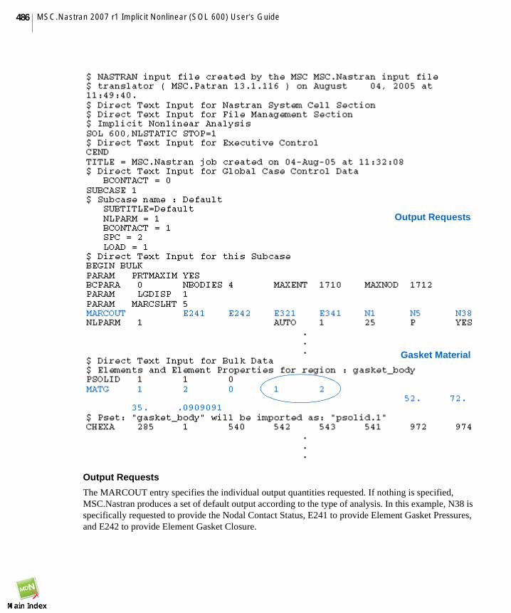
MSC.Nastran 2007 r1 Implicit Nonlinear (SOL 600) User’s Guide486
Output Requests
The MARCOUT entry specifies the individual output quantities requested. If nothing is specified,MSC.Nastran produces a set of default output according to the type of analysis. In this example, N38 isspecifically requested to provide the Nodal Contact Status, E241 to provide Element Gasket Pressures,and E242 to provide Element Gasket Closure.
Output Requests
Gasket Material

487CHAPTER 13SOL 600 Example Problems
Gasket Material
The MATG entry defines the gasket material properties. Highlighted in the circle, “1” is the table ID forthe loading path and “2” is the table ID for the unloading path. Additional properties including yieldpressure, tensile modulus, transverse shear modulus, and the initial gap, follow the table IDs.
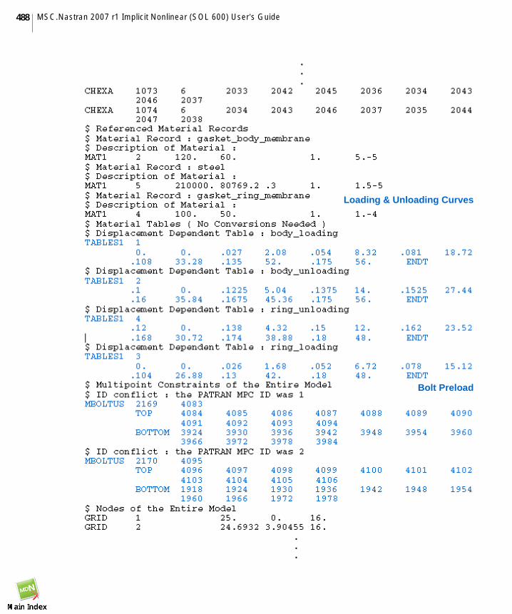
MSC.Nastran 2007 r1 Implicit Nonlinear (SOL 600) User’s Guide488
Loading & Unloading Curves
Bolt Preload

489CHAPTER 13SOL 600 Example Problems
Loading & Unloading Curves
The TABLES1 entries define the loading and unloading paths for the gasket body and gasket ring.
Bolt Preload
The two MBOLTUS entries define a set of grids through the cross-section of each bolt and identify acontrol grid which will be associated with enforced displacements.
Enforced Displacements
The FORCE and SPCD entries are used to enforce a displacement on the control grids that were specifiedin the MBOLTUS entries above.
Inspecting the ResultsThis example examines the gap closure and pressures generated around the circumference of the gasketdue to an imposed initial displacement on the two connecting bolts.
Enforced Displacements

MSC.Nastran 2007 r1 Implicit Nonlinear (SOL 600) User’s Guide490
Results Files
As an alternative to recreating the analysis model and running the analysis, you may access the generatedresults file as follows:
• gasket.marc.out - results file that can be opened in a text editor.• gasket.marc.t16 - accessible in MSC.Patran from the gasket.db.
Results Plots
The fringe plot of pressure shows an uneven pressure distribution around the circumference of the gasketring with larger pressures concentrated around the bolts.
The simulated gap closure

491CHAPTER 13SOL 600 Example Problems
Elastic-Plastic Collapse of a Cylindrical Pipe underExternal Rigid Body Loading
Problem StatementA model of a cylindrical pipe is subjected to crushing as rigid bodies above and below the pipe moveinward toward each other. The model is created using 2D shell elements to model the pipe, and rigidsurfaces above and below the pipe. This exercise illustrates several SOL 600 capabilities including largedisplacement analysis, contact analysis between rigid and deformable bodies, and plasticity modeledwith an elastic - perfectly plastic model.
The Structure and its Application
This problem examines a section of steel pipe eight inches in diameter and 24 inches long with a wallthickness of 0.4 inches. Steel pipes of this size are often used in land-based and offshore oil and gasindustries. Individual pipe sections are assembled with threaded connectors to form large pipelinedistribution systems. The pipe sections and their connections must withstand installation and operationalloads. The effects of these loads can be buckling, torque, bending, axial separation, external pressure,and internal pressure. In addition to environmental loads, surrounding structures undergoingdisplacement can introduce contact conditions. Forces from these external structures can also lead tointolerable failure scenarios.
Pipe design typically looks at all foreseeable failure scenarios and then a design is measured against thefailure mode that is most critical to structural integrity. In most cases that failure mode is bendingcombined with axial forces while under external pressure (if submerged) and internal pressure (fluidflow). However, in this case we examine failure due to external loading from adjacent structures.
In this problem the pipe section is subjected to offset lateral loading from external structures on the topand bottom. The problem attempts to quantify whether the movement of these external structures cause

MSC.Nastran 2007 r1 Implicit Nonlinear (SOL 600) User’s Guide492
the plastic collapse of the pipe. Initial contact with the external structures is expected to cause elasticdeformation of the steel pipe. Additional incremental movement potentially subjects the structure tostresses beyond the proportional limit of the material. The yield stress defines the onset of plastic strainsthat may initiate the collapse of the structure walls.
This example illustrates several of the capabilities in SOL 600 including large displacement analysis,contact analysis of a deformable body by rigid body movement, and material plasticity modeled with anelastic - perfectly plastic model. The resulting deformation data can establish the conditions forcatastrophic collapse of the pipe section and define allowable limits to contact of external structures.
Model DescriptionThe model includes a 3-D representation of the deformable pipe structure and two semi-circular sectionsof rigid pipes sections.
Geometry and Contact Regions
The primary structure is a continuous linear section of pipe 24 inches long with a diameter of 8 inchesand a homogeneous wall thickness of 0.4 inches. The pipe surface is void of attachments, holes, bends,or other discontinuities and the internal volume is empty space. Two external pipe structures are orientedin a perpendicular direction and lie directly on the top and underneath the primary pipe. The bottom pipemeasures 6 inches in diameter with a length of 10 inches and the top pipe measures 8 inches in diameteralso with a length of 10 inches.
The external pipe structures that lie directly on top and bottom surface of the primary pipe impose noinitial displacement or force, and no conditions are assumed to exist that might cause friction or slippageat the interface. These external structures move laterally into the pipe section creating a “sandwiching”effect. The pipe movement causes deformations on both the upper and lower side of the pipe.
Finite Element and Contact Model
Actual sections of oil and gas pipes can extend past 30 feet. Lengths beyond the 24-inch section modeledin this problem are assumed be irrelevant in the local collapse of the pipe wall. Each end of the pipe modelis assigned boundary conditions to represent the extension of the pipe in both directions. In addition, thepipe wall is sufficiently thin so that it is modeled with thick shell elements in this problem.
The finite element mesh for the primary pipe structure contains 18 elements around the circumferenceand 18 elements along the length for a total of 324 elements. MSC.Nastran CQUAD4 elements areselected along with the PSHELL entry that accounts for standard membrane, bending and transverseshear behavior. All shell elements are assigned a thickness of 0.4 inches, designated with 5 layers, anddefined to be the steel material.
In defining the contact model, the primary pipe section is modeled as a deformable body and the twoexternal pipe structures are modeled as rigid bodies. Elements comprising the deformable pipe structureare flagged so that contact by a rigid body creates forces that are used to calculate the deformation of thepipe. The rigid body structures do not deform and their movement is described with the BCBODY option.

493CHAPTER 13SOL 600 Example Problems
The geometry profile of the rigid surface is defined using 3D NURB surfaces that describe the truesurface geometry and most accurately represent the curved surfaces.
Material
The entire pipe section is made of steel and modeled as an elastic-plastic material using the MAT1 andMATEP entries for large displacement analysis. The linear elastic behavior model is effective up to ayield stress of 36000psi. In this range imposed stresses induce linear proportional strains. The stress-strain relationship is defined using an elastic modulus of 3.0E+6 and a Poisons ratio of 0.3. Beyond theyield point perfect plasticity causes complete yielding of the material upon any incremental stress.
Solution Procedure and Controls
A static analysis is performed to determine the pipe deformations that result from contacting rigid bodies.The rigid body movement and material stiffness specified for this problem require that largedisplacement effects be included (PARAM LGDISP).
Rigid body movement is spread over multiple load increments to allow for the history-dependent natureof the material response. Thus the equilibrium state and material state at the end of the first incrementconstitutes the beginning state for the second increment. The automatic load increment option(NLAUTO) is used to control the magnitude of the load increment. The initial time increment is set at.01 sec. The total load is 2 inches of imposed rigid body lateral movement on the top and bottom of thepipe occurring over 1 sec.
Within each increment an iterative process obtains an equilibrium state. Iterations are based on the FullNewton-Raphson method with a desired number of iterations per increment being 3, and a maximum setat 2500. Convergence for each increment is defined based on relative residual forces of less than 0.1.
Output requests are made for four stress-strain components using the MARCOUT entry. Total strainstensor, stress tensor, plastic strain tensor, and Cauchy stress tensor are requested to be included in thet16 file.
Loading and Boundary Conditions
Because only a small section of the pipe is modeled, the ends of the pipe are constrained in alltranslations. This boundary condition effectively represents the pipe extending a substantial distance inboth directions in which case no translation movement would occur at this section’s boundary.
To model the contact, the top and bottom rigid surfaces are given velocity vectors of –2 in/sec., and+2 in/sec. respectively in the y-direction (lateral). This causes the upper structure to be pushed onto thetop of the pipe section and the lower structure to be pushed up into the bottom of the pipe section at arate of 2 in/sec. for a total time of 1 second.

MSC.Nastran 2007 r1 Implicit Nonlinear (SOL 600) User’s Guide494
Solving the ProblemThe pipe crush example is designed to be constructed and setup using MSC.Patran and analyzed usingMSC.Nastran SOL 600. The geometry is constructed and then property/load assignments are made inMSC.Patran. A MSC.Nastan Bulk Data file (bdf) is exported and then run with MSC.Nastran. Resultscan be accessed in text form or from inside MSC.Patran and processed for viewing the pipe deformationsand stresses.
Input Files Required• None
Recreating the Problem using MSC.Patran
Step-by-step instructions for creating and running the analysis on the pipe crush model can be accessedby linking to the pipe_crush instructions file below. Once you are done creating the model and runningthe SOL 600 analysis, proceed by accessing the results file to generate visual displays of the simulateddeformations and stresses.
Click here for Pipe Crush Modeling Instructions
Highlighted Sections of the MSC.Nastran Bulk Data File
The following sections of the MSC.Nastan Bulk Data file highlight the SOL 600entries generated fromthe problem setup described above.
Move 2 in the Y
R=4
R=3
Move 2 in the -Y
Pipe
Rigid Body 2
Rigid Body 1
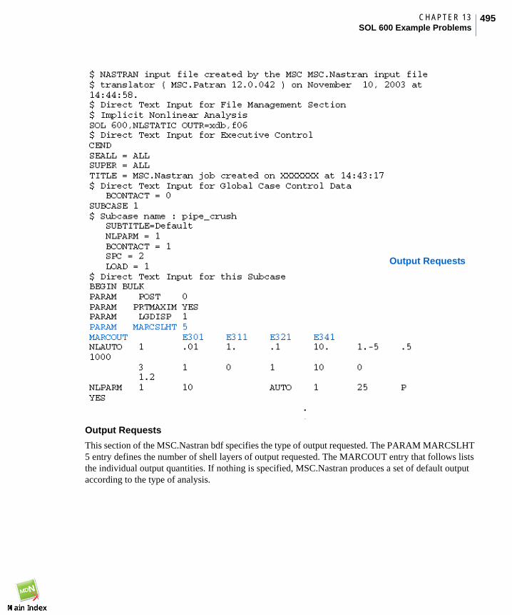
495CHAPTER 13SOL 600 Example Problems
Output Requests
This section of the MSC.Nastran bdf specifies the type of output requested. The PARAM MARCSLHT5 entry defines the number of shell layers of output requested. The MARCOUT entry that follows liststhe individual output quantities. If nothing is specified, MSC.Nastran produces a set of default outputaccording to the type of analysis.
Output Requests

MSC.Nastran 2007 r1 Implicit Nonlinear (SOL 600) User’s Guide496
Material Entries
This section of the MSC.Nastran bdf describes the material behavior for the pipe. The MAT1 entrydefines the elastic part of the material and the MATEP entry describes the perfectly plastic behavior.
Contact Bodies
The BCBODY entry describes the rigid surface as defined by Nurbs geometry surfaces. The value of“analytical form” is 1 (used with all Nurbs rigid geometry). Note the -2 describing the rigid body motion.
Material Entries
Contact Bodies

497CHAPTER 13SOL 600 Example Problems
Inspecting the Results
Results Files
The .sts file shown below reports on the status of the run. In this problem the run completed withouterrors. Using the adaptive load incrementation algorithm the solution was obtained with 27 loadincrements. Two increments required 22 and 24 iterations to converge.
Adaptive Load Incrementation

MSC.Nastran 2007 r1 Implicit Nonlinear (SOL 600) User’s Guide498
Adaptive Load Incrementation
The adaptive load incrementation algorithm adjusts the time step size according to the number ofiterations required to achieve convergence on the preceding increment. In this example the 10thincrement required 22 iterations to obtain convergence. The time step between the 10th and 11thincrement was subsequently adjusted downward and convergence on the 11th increment was reduced tonine iterations. A similar situation arose in the 16th increment.
Results Plots
Figure 13-1 shows the final deformed shape of the pipe section after 1 sec. of loading. Maximum totalstrains of 6.0E-2 inches develop in rigid body contact areas. Slightly higher total strains are evident onthe lower pipe section in this region due to the difference in radius of the external rigid body structures.
Plasticity has occurred over most of the model as shown in Figure 13-2. Maximum stresses reaching4.25E+4 psi occur as expected in the contact region. Also evident from this figure are high stressesequivalent to those in the contact region occurring at the constrained boundary condition. This is aconsequence of the boundary condition. In a full-length pipe section we would not expect to see a stressconcentrated in this area.
Figure 13-1 Total Strains imposed on the Deformed Shape

499CHAPTER 13SOL 600 Example Problems
Figure 13-2 Deformed Shape and Stress Distributions

MSC.Nastran 2007 r1 Implicit Nonlinear (SOL 600) User’s Guide500
Rubber Door Seal - Performance Door Closing
Problem StatementThis problem illustrates the nonlinear analysis of a trunk door rubber seal. The simulation highlightsseveral SOL 600 capabilities including hyperelastic material, large displacement, large strain, and contactbetween rigid and deformable bodies.
The Structure and its Application
This problem examines the behavior of a rubber seal under a closing trunk door. The rubber seal has anouter diameter of 1.25” and a wall thickness of 0.125”. It is modeled using plane strain elements withhyperelastic material formulation. While the door is closing, the trunk door comes in contact with therubber seal and deforms it. The deformation of the seal needs to be examined to make sure it properlyseals the door when the door is closed.
Model DescriptionThis model consists of a planar representation of the rubber seal and a curve representation of the door.The rubber seal and door are initially located approximately 0.1” apart.

501CHAPTER 13SOL 600 Example Problems
Geometry
This three-dimensional problem is idealized as a plane strain problem. The rubber seal geometry isrepresented by several surfaces. The trunk door is represented by several curves.
Finite Element and Contact Model
The surfaces representing the seal are meshed with MSC.Nastran CQUD4 shell elements. The elementproperty is defined using the nonlinear hyperelastic plane strain property entry PLPLANE. All the sealCQUAD4 elements are defined as a single deformable body using the BCBODY and BSURF entries.
The curves representing the trunk door are used to define a rigid contact body using the BCBODY entry.The NURBS2D option is used to describe the rigid body geometry.
Material
The rubber seal material is defined using the Mooney Rivlin material model. The MSC.Nastranhyperelastic material property entry MATHP is used with two material constant terms: A10=80 andA01=20.
Loading and Boundary Conditions
Nodes along the bottom edge of the seal are fixed. A displacement of (-0.1, -0.7, 0.) is specified on therigid body to control the motion of the rigid body.
Solution Procedure and Controls
A nonlinear static analysis is performed to determine the seal deformations that result from contact withthe rigid trunk door. The rigid body movement and material stiffness specified for this problem requirethat large displacement effects be included (PARAM,LGDISP,1).
The NLPARM entry is used to specify the nonlinear analysis iteration strategy. 10 uniform timeincrements are used to solve this problem. The Full Newton-Raphson method is specified.
Output requests are made for stress and strain using the MARCOUT entry. These results are included inthe t16 output file.
Solving the ProblemThe rubber seal problem is designed to be constructed and setup using MSC.Patran and analyzed usingMSC.Nastran SOL 600. First, the geometry is created in MSC.Patran by running a session file. Next theseal geometry is meshed in MSC.Patran to generate shell elements. Then property/loads/BC assignmentsare made in MSC.Patran. A MSC.Nastan Bulk Data file (bdf) is exported and then run withMSC.Nastran. Analysis results can be accessed in text format or viewed from inside MSC.Patran.
Input Files Required• rubber_seal.ses - MSC.Patran session file containing commands to build the rubber seal and
trunk door geometry.

MSC.Nastran 2007 r1 Implicit Nonlinear (SOL 600) User’s Guide502
Recreating the Problem using MSC.Patran
Step-by-step instructions for creating and running the analysis on the rubber door seal model can beaccessed by linking to the Rubber Door Seal Modeling Instructions file below. Once you are donecreating the model and running the SOL 600 analysis, proceed by accessing the results file to generatevisual displays of the analysis results.
Click here for Rubber Door Seal Modeling Instructions

503CHAPTER 13SOL 600 Example Problems
Highlighted Sections of the MSC.Nastran Bulk Data File
Large Displacement
Hyperelastic Material Entries
Contact Definition

MSC.Nastran 2007 r1 Implicit Nonlinear (SOL 600) User’s Guide504
Inspecting the Results
Results Files
The .sts file shown below reports on the status of the run. Using the fixed load incrementation algorithm,the job was completed in 10 equal time increments
.
Results Plots
The plot below shows the final deformation and strain results.

505CHAPTER 13SOL 600 Example Problems
Brake Forming
Problem StatementThis problem illustrates the nonlinear analysis of a flat steel plate being formed into an angled bracket.A cylindrical punch is used to bend the plate by pushing it into a die, then retracting away. This formingprocess is commonly known as brake forming.
This simulation highlights several SOL 600 capabilities including multiple load steps, material plasticity,large displacement, large strain, and contact between rigid and deformable bodies.
The Structure and its Application
This problem examines the behavior of a flat steel plate undergoing metal forming. The plate is 1.8” wideand 0.1” thick. The punch has a 2.0” diameter. The plate is modeled using plane strain elements. Sincethe plate will be deformed beyond its material yield point, an elastic-plastic material model will be usedto simulate the material yielding behavior. The forming process consists of two steps. In the first step,the punch pushes the plate into the die, causing it to deform plastically. In the second step, the punch isretracted away from the plate.
Model DescriptionThis model consists of a planar representation of the plate and curve representations of the punch and die.
Geometry
This three-dimensional problem is idealized as a plane strain problem. The plate is represented by asurface. The punch is represented by a circular curve. The die is represented by a composite curve.

MSC.Nastran 2007 r1 Implicit Nonlinear (SOL 600) User’s Guide506
Finite Element and Contact Model
The surface representing the plate is meshed with MSC.Nastran CQUAD4 shell elements. The elementproperty is defined using the PSHELL entry with MID2 set to -1 to specify the plane strain option. Allthe plate CQUAD4 elements are defined as a single deformable body using the BCBODY and BSURFentries.
The circular curve representing the punch is used to define a rigid contact body using the BCBODY entry.The composite curve representing the die table is used to define a second rigid contact body using theBCBODY entry. The NURBS2D option is used to describe the geometry for both rigid bodies.
Material
The plate is made of steel and modeled as an elastic-plastic material using the MAT1 and MATEP entries.The linear elastic behavior model is effective up to a yield stress of 50000 psi. In this linear range thestress-strain relationship is defined using an elastic modulus of 30E+6 and a poisson ratio of 0.3. Theplastic stress-strain relationship is defined by 7 pairs of stress-strain values using the TABLES1 entry.
Loading and Boundary Conditions
The nodes along the centerline of plate are fixed in the lateral direction to prevent the plate from driftingsideways. A one-G gravitational acceleration is applied to the plate to hold the plate against the die table.
The die table rigid body is held stationary. An enforced vertical displacement of -0.3” is applied to thecontrol node of the punch rigid body during the first load step. In the second load step, an enforcedvertical displacement of zero is applied to the same control node to return the punch to its initial position.
Solution Procedure and Controls
A nonlinear static analysis is performed to determine the steel plate deformations and stresses that resultfrom the brake forming process. The rigid body movement and material stiffness specified for thisproblem require that large displacement effects be included (PARAM,LGDISP,1).
The adaptive load increment option is used with an initial time size of 0.01. Output requests are made forstress and strain using the MARCOUT entry. These results are included in the t16 output file.
Solving the ProblemThe brake forming problem is designed to be constructed and setup using MSC.Patran and analyzedusing MSC.Nastran SOL 600. First, an IGES geometry file is imported into MSC.Patran. Next the plategeometry is meshed in MSC.Patran to generate shell elements. Then property/loads/BC assignments aremade in MSC.Patran. A MSC.Nastan Bulk Data file (bdf) is exported and then run with MSC.Nastran.Analysis results can be accessed in text format or viewed from inside MSC.Patran.
Input Files Required• brake_forming_s600.igs - IGES file containing plate, punch, and die geometry.

507CHAPTER 13SOL 600 Example Problems
Recreating the Problem using MSC.Patran
Step-by-step instructions for creating and running the analysis on the brake forming model can beaccessed by linking to the Brake Forming Modeling Instructions file below. Once you are done creatingthe model and running the SOL 600 analysis, proceed by accessing the results file to generate visualdisplays of the analysis results.
Click here for Brake Forming Modeling Instructions

MSC.Nastran 2007 r1 Implicit Nonlinear (SOL 600) User’s Guide508
Highlighted Sections of the MSC.Nastran Bulk Data File
Defining Subcases for Multiple Load Steps
Large Displacement
Plasticity
Contact

509CHAPTER 13SOL 600 Example Problems
Inspecting the Results
Results Plots
The plot below shows the analysis results at the end of the forming operation.

MSC.Nastran 2007 r1 Implicit Nonlinear (SOL 600) User’s Guide510
Panel Buckling
Problem StatementThis problem illustrates the nonlinear post-buckling analysis of a curved panel. This simulationhighlights several SOL 600 capabilities including large displacement, material plasticity, and contactbetween multiple deformable bodies.
The Structure and its Application
Panels constructed from thin sheets reinforced with stiffeners are commonly used in many industries.In order to keep these panels light, the thin sheet (skin) is often designed to be thin and allowed tobuckle elastically at relatively low levels of compressive loading. Once the skin buckles, thecompressive load distribution changes in the panel, and any additional load is carried mostly by thestiffeners. The final failure load is reached when the overall panel fails due to a combination of materialyielding and instability.
MSC.Nastran SOL 600 provides the capabilities required to simulate this panel post-buckling behavior.
Model DescriptionThe model consists of a stiffened panel approximately 14” by 22”. The skin is constructed fromaluminum and has a slight curvature. A longitudinal Z stiffener is attached to the skin by a single row ofrivets. The stiffener has a joggle in it, and a doubler is used to fill the gap between the stiffener and theskin. Two additional longitudinal doublers are attached to the outside edges of the skin.
This model was originally constructed in metric units and was converted to English units. As a result ofthe conversion, some of the dimensions are rounded off.

511CHAPTER 13SOL 600 Example Problems
Geometry and Contact Regions
The skin, stiffener, and doublers are all modeled as shell elements located at the mid-surface of thesecomponents. The gap between two components is equal to half the thickness of one component plus halfthe thickness of another component. These components are allowed to contact each other.
Finite Element and Contact Model
The skin, stiffener, and doublers are modeled using CQUAD4 elements. The element properties aredefined using PSHELL entries.
The rivets are modeled using CBAR elements. The element property is defined using the PBAR entry.
The three doublers are modeled as three deformable contact bodies. The stiffener lower flange is definedas a deformable contact body. The skin is in contact with several components. Each contact area withinthe skin is defined as a deformable contact body.
An RBE2 rigid body element is used to connect all the nodes on one end of the panel to a single node.This node is used to apply the panel loading.
Material
The skin and doublers are made of aluminum alloy 2024 which is modeled as an elastic-plastic materialusing MAT1 and MATEP entries. The stiffener is made of aluminum alloy 7349 and is also modeled asan elastic-plastic material using MAT1 and MATEP entries. The plastic stress-strain relationships aredefined by pairs of stress-strain values using TABLES1 entries.
Loading and Boundary Conditions
All the nodes on one end of the panel are fixed in all six degrees of freedom. At the other end of the panel,an RBE2 rigid body element connects the nodes to a single node, and an enforced displacement of 0.28”in the longitudinal direction is applied to this node.
The longitudinal edges of the panel are fixed in the lateral directions but are free to slide in thelongitudinal direction.
Solution Procedure and Controls
A nonlinear static analysis is performed to determine the capability of the panel to support a compressiveload. PARAM,LGDISP,1 is specified to activate the large displacement capability.
The NLPARM and NLSTRAT entries are used to specify the nonlinear analysis iteration strategy. 40fixed time increments are specified for this problem. Output requests are made for stress and strain usingthe MARCOUT entry. These results are included in the t16 output file.

MSC.Nastran 2007 r1 Implicit Nonlinear (SOL 600) User’s Guide512
Solving the ProblemThe panel post-buckling problem is designed to be constructed and setup using MSC.Patran and analyzedusing MSC.Nastran SOL 600. A MSC.Patran database is provided which contains the complete finiteelement model. A MSC.Nastan Bulk Data file (bdf) is exported and then run with MSC.Nastran. Analysisresults can be accessed in text format or viewed from inside MSC.Patran.
Input Files Required• stiffened_panel.db - MSC.Patran database containing the panel finite element model.
Recreating the Problem using MSC.Patran
Step-by-step instructions for creating and running the analysis on the panel buckling model can beaccessed by linking to the Panel Buckling Modeling Instructions file below. Once you are done creatingthe model and running the SOL 600 analysis, proceed by accessing the results file to generate visualdisplays of the analysis results.
Click here for Panel Buckling Modeling Instructions

513CHAPTER 13SOL 600 Example Problems
Highlighted Sections of the MSC.Nastran Bulk Data File
Plasticity
Contact
Large Displacement

MSC.Nastran 2007 r1 Implicit Nonlinear (SOL 600) User’s Guide514
Inspecting the Results
Results Plots
The plot below shows the final deformation of the panel.
The plot below shows a graph of the total longitudinal reaction force vs. time increments.