msc in applied mathematics

Title: On the length spectrum of analytic convex billiard tables Author: Anna Tamarit Sariol Advisors: Pau Martín de la Torre and Rafael Ramírez Ros Department: Matemàtica Aplicada 1 Academic year: 2010-2011

MSc in Applied Mathematics

Universitat Politecnica de Catalunya

Facultat de Matematiques i Estadıstica

Master Thesis

On the length spectrum of analytic

convex billiard tables

Anna Tamarit

Advisors: Pau Martın and Rafael Ramırez

Departament de Matematica Aplicada 1

Al Pau i al Rafa, per ser positius i sempre estar

predisposats a ajudar

Abstract

Key words: Area-preserving twist maps, billiards, length spectrum, Melnikov, exponen-tial smallness, periodic orbits

MSC2000: 37E40, 37J10, 37J40

Billiard maps are a type of area-preserving twist maps and, thus, they inherit a vast num-ber of properties from them, such as the Lagrangian formulation, the study of rotationalinvariant curves, the types of periodic orbits, etc. For strictly convex billiards, there existat least two (p, q)-periodic orbits. We study the billiard properties and the results foundup to now on measuring the lengths of all the (p, q)-trajectories on a billiard. By usinga standard Melnikov method, we find that the first order term of the difference on thelengths among all the (p, q)-trajectories orbits is exponentially small in certain perturba-tive settings. Finally, we conjecture that the difference itself has to be exponentially smalland also that these exponentially small phenomena must be present in many more casesof perturbed billiards than those we have presented on this work.

Contents

Introduction 1

Part 1. State of the art 5

Chapter 1. Area-preserving twist maps 71.1. Basic definitions 71.2. Rotational invariant circles 91.3. Generating function and variational formulation 101.4. Periodic orbits 131.5. Rotation number of twist maps 15

Chapter 2. Billiards 192.1. The model 192.2. Properties 222.3. Convex caustics and rotational invariant circles 262.4. Billiards inside a circle 282.5. Elliptic billiards 30

Chapter 3. General tools 353.1. Birkhoff normal form 353.2. Moser’s Twist Theorem 373.3. Melnikov potential for perturbations of area-preserving twist maps 40

Chapter 4. Specific results of perturbative theory 434.1. An example of exponentially small phenomena: upper bound of the

splitting of invariant curves 434.2. Existence of caustics near the billiard boundary 444.3. Break-up of caustics 464.4. Length spectrum of convex domains 47

Part 2. Goals and first results 49

Chapter 5. Discussion of problems to treat 515.1. Introduction to the problems 515.2. Our approach 52

Chapter 6. First results 556.1. Circular tables 55

ix

x CONTENTS

6.2. Elliptic tables 60

Conclusions and further problems 69

References 71

Appendix A. Billiard map for a small incidence-reflexion angle 73

Appendix B. Elliptic functions 77B.1. Jacobian elliptic functions 80B.2. Elliptic sinus 81B.3. Elliptic cosinus 82

Introduction

Birkhoff [6] introduced the problem of convex billiard tables to describe a motionof a free particle inside a closed convex curve. The motion follows the law “theangle of incidence equals to the angle of reflection”. Billiards are a simple con-cept which already contains some of the most important questions on dynamics.Birkhoff already reflected this idea when saying “in the billiard problem the formalside, usually so formidable in dynamics, almost completely disappears and only theinteresting questions need to be considered”[6, p.170].

The billiard motion can be modeled by an area-preserving twist map on an opencylinder. This characterization is useful in different settings.

On the one hand, the twist condition characterizes the rotational invariant circles,RICs, as graphs of a function defined on the angular coordinate (Birkhoff The-orem [20, §IV]). As invariant structures, it is interesting to study the restricteddynamics. Since they are conjugate to a circle diffeomorphism, a rotation numbercan be associated to each RIC. For an integrable area-preserving twist map, all theRICs with a Diophantine rotation number are preserved under small perturbation.This perturbative result is due to Moser [25, §32,33] and it is part of the KAMtheory.

On the other hand, area-preserving twist maps admit a variational principle which isanalogous to the Lagrangian-action formulation of analytical mechanics. Orbits arestationary points of the action functional and the minima and minimax points leadto a class of orbits that are of great importance. In particular, for (p, q)-periodicorbits, the minima and minimax points, different in nature, imply the existence ofat least two (p, q)-periodic orbits (Poincare Birkhoff Theorem [20, §VI]).

In the billiard setting, the action coincides with the sum of the length of the chordsbetween two consecutive impact points. Also, in the billiard table, (p, q)-periodicorbits correspond to polygons of q sides making p turns inside the boundary of thetable and its rotation number is p/q.

The existence of RICs on the billiard map is closely related to a curve called caus-tic inside the table. A caustic has the property that once a trajectory is tangentto it, it stays tangent to the caustic after every reflection. We can associate tworotational invariant curves on the phase space to each convex caustic and also a

1

2 INTRODUCTION

rotation number. The existence of convex caustics with Diophantine rotation num-bers is guaranteed close to the billiard table boundary [17]. Also, their existenceis guaranteed for any trajectory in the circular and elliptic billiards as these mapsare Liouville integrable and convex caustics are related to RICs.

In the context of circular and elliptic maps, since the (p, q)-periodic orbits are acontinuous family on a RIC, all the trajectories have the same length. Contrary toDiophantine RICs, these resonant RICs generically break up under arbitrarily smallperturbations. Thus, the length of the different (p, q)-periodic orbits is not same andone can try to measure the maximum difference. The attempts on this measurerely on a Melnikov method [24][22]. The Melnikov technique is based on thestudy of the lower order terms on a Taylor expansion according to the perturbativeparameter. When not only the perturbative parameter tends to zero but also theperiod tends to infinity, the lower order terms might be not the important ones andall the terms have to be taken into account. In these situations, the literature (see[8] for instance) has always turned to the study of the Birkhoff normal form [25,§23].

There exist results on the maximum difference among all the (p, q)-periodic orbitsnot only for Liouville integrable maps but for any strictly convex smooth billiard.The difference is beyond any order with respect to q when the (p, q)-periodic orbitsare approaching to the boundary [18], or close to an elliptic (1, 2)-periodic orbit [8].Taking these results to an analytic context leads to think that this maximum dif-ference will be exponentially small, as it happens in other problems [11].

This memoir is a first step on the study of the length of the periodic orbits existingin any convex billiard which has to be continued in the next years. In Part 1, wegive a complete review on the necessary concepts surrounding our matter of subjectand we also highlight the existing results on the length spectrum of billiards. AtPart 2 we develop some of the tools exhibited in order to give some first results invery concrete settings.

Part 1, State of the art, is divided into four different chapters. Chapter 1 compilesthe most important notions on area-preserving maps while in Chapter 2 we focuson the billiard map and its the geometric properties. We will pay special attentionto the circular and elliptic billiards. Chapters 1 and 2 mainly follow [20] and [14].Further information on billiards can be found in [15], [26], [16] and [6].

In Chapter 3, we review some tools used on dynamical systems when studyingthe effect that small perturbations cause on the unperturbed invariant sets. Inparticular we review the Moser’s Twist Theorem [25, §32,33] and the Melnikovsubharmonic potential [22]. We also review the Birkhoff normal form [25, §23].

Finally, Chapter 4 gives the State of the art results we are based on to start ourstudy. Results on exponentially small phenomena [11], the existence of caus-tics [17], the break up of resonant tori [24][22] and the length spectrum [18][8]are given.

Part 2 focusses on delimiting the subject studied and showing some first results.In Chapter 5 we discuss the problem we want to study and the approach we willbe following. The results obtained when applying the proposed method to generic

INTRODUCTION 3

perturbations of the billiard on the circle and some particular ones on the ellipseare shown on the last chapter.

Part 1

State of the art

Chapter 1

Area-preserving twist maps

1.1. Basic definitions

We will consider diffeomorphisms defined on an open cylinder of the form C = T×Y ,

T = R/Z and Y = (y−, y+) ⊂ R. Its universal cover, C = R× Y , is a strip of theplane. We will use coordinates (s, y) for C and same coordinates with a tilde,

(s, y) for C. In fact, the tilde will always denote the lift of a point, a functionor a set to the universal cover. Horitzontal and vertical directions will be calledthe angular and radial directions respectively. The image of a point (s, y) will bedenoted by (s1, y1).

Definition 1.1.1. A lift F of a map T : C → C is a map F : C → C such that if

π : C → C is the projection to the quotient space C, then the following diagramcommutes,

CF→ C

↓π ↓πC

T→ C

Immediate consequences of this definition are the following. Let T = (T1, T2) andF = (F1, F2). Then, F1 commutes with integer shifts in the angular direction whileF2 is 1-periodic in the first variable.

Observe that for F and G lifts of T , F −G ≡ (k, 0), k ∈ Z. In general, we will fix

the lift, T , in such a way that T (0, 0) ∈ [0, 1)× Y .

Definition 1.1.2. A diffeomorphism T : C → C of the open cylinder to itself iscalled an area-preserving twist map if

(1) T preserves area,(2) T preserves orientation,(3) T preserves boundary components, and

(4) its lift T : C → C has the twist property: ∂2T1(s, y) 6= 0, where ∂2 denotes thederivation with respect the second variable.

Remark 1.1.1. If the map could be continuously extended to the closed cylinderT : T× Y → T× Y , the preservation of the boundary components will be nothing

7

8 1. AREA-PRESERVING TWIST MAPS

but the condition T (T × y−) = T × y− and T (T × y+) = T × y+. Ifthis extension is not possible, the condition of the preservation of the boundarycomponents can be written as ∃ε > 0 such that T (T× (y−, y− + ε)) ⊂ T× (y−, y)and T (T× (y+ − ε, y+)) ⊂ T× (y, y+), where y = (y+ + y−)/2.

Remark 1.1.2. We say that T twists to the right if T1 is a monotonically increasing

function of y and T twists to the left if T1 decreases monotonically with y.

Observe that the inverse of an area-preserving twist map is also an area-preservingmap, but with the twist twisting to the opposite direction. Therefore, and since atwist map is a diffeomorphism, with no loss of generality, we will be working withtwist maps twisting to the right while the results will apply to any twist map.

It is worth to remark that the set of twist maps is not a group under the composition.The reason is that the composition of two twist maps can make some points rotateso much that their second iterates could violate the twist condition.

Definition 1.1.3. The twist interval of T is the set of numbers α ∈ R for whichthere exists ε > 0 such that if (s, y) ∈ R× (y−, y− + ε) then T1(s, y)− s ≤ α and if

(s, y) ∈ R× (y+ − ε, y+) then T1(s, y)− s ≥ α. It is denoted by (ω−, ω+).

Observe that the twist interval is defined as a set. But, any number between twonumbers belonging to the twist interval also belongs to it and therefore it is indeedan interval.

Also, the interval is well defined up to integer translation so we will define it in theinterval (0, 1).

As before, if the map can be continuously extended to the closed cylinder, the twist

interval is(limn→∞(T n

1 (s, y−)− s)/n, limn→∞(T n1 (s, y+)− s)/n

). These limits of

the interval are related to the rotation number of the restriction of the diffeomor-phism on both cylinder covers. In Section 1.5, more information on the rotationnumber of a map on a circle can be found.

If T is a twist map with lift T and ∂2T1 is bounded away from 0, then any sufficiently

small C1-perturbations of T is also a twist map. Furthermore, the endpoints of thetwist interval depend continuously on the perturbation.

A particular type of area-preserving twist maps are of the following form.

Definition 1.1.4. An area-preserving twist map is called integrable if it is of theform T (s, y) = (s+ g(y), y).

Integrable twist maps leave circles T×y invariant and rotate them by g(y), whichhas to be a monotone function. They are foliated by rotational invariant circles (aswe explain in the next section, invariant curves not contractible to a point arecalled this way). Also, we can observe that for each rational value of g we havea continuous family of periodic orbits separated by circles with irrational rotationnumber. The twist interval is (limy→y−

g(y), limy→y+g(y)).

1.2. ROTATIONAL INVARIANT CIRCLES 9

1.2. Rotational invariant circles

Definition 1.2.1. A rotational invariant circle (RIC) is a closed loop Υ homotopi-cally non trivial such that T (Υ ) = Υ .

A rotational invariant circle divides the cylinder into two invariant regions. To seethis, consider A the region of the cylinder below the RIC and consider its image,T (A). Since T is a continuous map, T (A) is a connected component. Since the RICis invariant and the boundaries are preserved, T (A) must have the same boundariesas A and since the map is bijective, T (A) = A. Therefore, RICs are barriers tomotion, they separe the phase space. In fact, a similar argument can be applied toany invariant closed curve, no matter if it is contractible to a point or not.

Birkhoff showed that any invariant set U that looks like “half a cylinder” has agraph-like boundary. Formally this result is written as follows.

Theorem 1.2.1 (Birkhoff Theorem, [20, §IV]). Let T be an area-preserving twistmap on the cylinder C. Let U be an open invariant set homeomorphic to the cylindersuch that there exist a, b ∈ Y , a < b satisfying T× (y−, a) ⊂ U ⊂ T× (y−, b). Then,the boundary of U is the graph (s, γ(s)) of some continuous function γ : T →(a, b).

Remark 1.2.1. In particular, the theorem implies that any invariant set U lookinglike “half a cylinder” can not have “whorls” on its boundary. See Figure 1.1.

Y

T

Fig. 1.1. The boundary drawn can not be a graph and thereforethe region below it is not invariant.

This result leads to some others which are often useful arguments when looking forRICs or its properties. We will now mention some.

Corollary 1.2.2. Any RIC is a graph.

Proof. We can consider U the region below the RIC, which we have already seenthat is invariant. Applying Birkhoff Theorem 1.2.1 we obtain that the RIC is agraph. ⊓⊔


Corollary 1.2.3 (Lipschitz corollary). The function γ is not only continuous butalso Lipschitz.

Proof. Let v = (0, δy) be a vertical vector at point (s, y) and let (δs1, δy1) beits image, (δs1, δy1) = DT (s, y)v. The slope of DT (s, y)v is S = δy1/δs1, δy1 =∂2T2(s, y), δs1 = ∂2T1(s, y). Since T is a twist map, δs1 has a positive lowerbound and there exists a maximum value for S, S+. Similarly, we can use that theinverse T−1 is also a twist map to find a lower bound for S, S−.

Therefore, we have found S− ≤ (γ(s)− γ(s′))/(s− s′) ≤ S+ for any s, s′ ∈ T andso γ is a Lipschitz function. ⊓⊔Corollary 1.2.4 (Confinement corollary). Suppose all the orbits of the points in(s, y) ∈ C, y < a stay below some circle T×b. Then, there exists a RIC betweeny = a and y = b.

Proof. To obtain this result, we construct a suitable set U satisfying the hypoth-esis of Birkhoff Theorem 1.2.1.

Consider the union of the orbits of the points below y = a. This set is invariant butit may have holes and may not satisfy requirements for the set U in the BirkhoffTheorem. Among the complement set, there is a connected component, V , whichcontains all the points above y = b. Take as set U the complement set to V : it isinvariant and all its points are below y = b. Then we can apply Birkhoff Theoremand proof the statement. ⊓⊔Corollary 1.2.5 (Non existence criterion). If there exists an orbit that is as closeas we want from both cylinder covers, T× y− and T× y+, there can not existany RIC.

Restricting the map T to the RIC, one obtains some interesting results on therestricted dynamics. These results are extracted from the study of homeomorphismsor diffeomorphisms on the circle. Since we also mention results about periodic orbitson the restricted dynamics, we have stated some of these results not in the nextsection but in Section 1.5.

1.3. Generating function and variational formula-

tion

We will show that any twist map verifies a Lagrangian variational principle. Thisvariational formulation is very useful to deduce properties or different types oforbits. We will see these applications in the next subsections.

Consider the area-preserving twist map T : (s, y) 7→ (s1, y1). We claim that thereexists a function H(s, s1) such that

y = −∂1H(s, s1),y1 = ∂2H(s, s1).

(1)

In fact we define it this way:

1.3. GENERATING FUNCTION AND VARIATIONAL FORMULATION 11

Definition 1.3.1. Let T be a lift of T . If (s, s1) ∈ R2 is such that T (s × Y ) ∩(s1 × Y ) 6= ∅, then, we denote by H(s, s1) the area of the region located to the

right and under T (s× Y ), to the left of s1× Y and above R× y−. FunctionH : (s, s1) 7→ H(s, s1) is called the generating function of T .

s s1

T

H(s, s1)

R

Y

Fig. 1.2. The generating function H(s, s1) is the area colored in

grey. It lies to the right and under T (s × Y ) and to the left ofs1 × Y .

Remark 1.3.1. If the twist map twisted to the left, H(s, s1) would be instead

defined as the area located to the left and under T (s×Y ), to the right of s1×Yand above R× y−.Remark 1.3.2. The twist condition implies that the intersection set T (s× Y )∩s1×Y is either void or is a single point, (s1, f1(s, s1)), for some uniquely defined

f1. Moreover, note that H(s+k, s1+k) = H(s, s1) since we know that T (s+k, y) =

T (s, y)+(k, 0). Therefore, functionH can be defined on the quotient spaceR×R/ ∼,where (s, s1) ∼ (t, t1) if and only if t = s+ k and t1 = s1 + k for some k ∈ Z.

If there exists (s1, f1(s, s1)) ∈ T (s×Y )∩(s1 × Y ) we can define a function f0 as

T−1(s1, f1(s, s1)) = (s, f0(s, s1)). Observe that we are saying that graph(f1(s, ·)) =T (s × Y ) and graph(f0(·, s1)) = T−1 (s1 × Y ).

From the definition of H(s, s1) as an area, we have H(s, s) = 0 and

H(s, s1) =

∫ s1

s

f1(s, ξ) dξ.(2)

Since T is area-preserving, the area of the preimage is the same and therefore, wealso have

H(s, s1) =

∫ s1

s

f0(ξ, s1) dξ.(3)

So if we have (s1, y1) = T (s, y) then f1(s, s1) = y1 and f0(s, s1) = y and equations(2) and (3) gives us the relation (1) since

y = f0(s, s1) = −∂1H(s, s1),y1 = f1(s, s1) = ∂2H(s, s1),


In fact, we can say something more.

Proposition 1.3.1 ([14, p. 342]). The generating function H determines the dy-namics uniquely.

Proof. We want to determine T1(s, y) and T2(s, y) from H(s, s1). We will applythe Implicit Function Theorem to

0 = F (s, s1, y, y1) :=

(∂2H(s, s1)− y1∂1H(s, s1) + y

).

We need that det(Ds1,y1F ) 6= 0,

det(Ds1,y1F ) = det

(∂11H(s, s1) −1∂12H(s, s1) 0

)= ∂12H(s, s1).

We know that ∂2H(s, s1) = f1(s, s1) and from the twist property we can deducethat, once fixed s1, f1(·, s1) is a decreasing function (see Figure 1.3). Therefore, at

any point, we have ∂12H(s, s1) < 0 and we can determine T (s, y) = (s1, y1). ⊓⊔

s s1

f1(s, s1)

z

f1(z, s1)

R

Y

Fig. 1.3. Once fixed s1, we apply T to sets z×Y and s×Y ,with z < s. The intersection point of both sets with the lines1 × Y is the definition of f1(z, s1) and f1(s, s1) respectively.Thus, we can observe that f1 is a decreasing function with respectto the first coordinate.

Thanks to the generating function we will be able to define a functional whosestationary points are orbits of the map. The following proposition gives a localresult.

Proposition 1.3.2 ([14, Proposition 9.3.4., p. 354]). Suppose s0 is a critical pointof s 7→ H(s−1, s) + H(s, s1). Then, there exist y−1, y0, y1 ∈ (y−, y+) such that

T (s−1, y−1) = (s0, y0) and T (s0, y0) = (s1, y1).

Remark 1.3.3 (About notation). Henceforth, the images and preimages of an ini-tial point (s0, y0) will be denoted, as done in the previous proposition, by (sn, yn) :=

T n(s0, y0) and (s−n, y−n) = T−n(s0, y0), respectively. Therefore, an orbit will bedescribed as . . . , (s−1, y−1), (s0, y0), (s1, y1), . . ..

This proposition gives a local result: a critical point s0 of a functional dependingon two other fixed values s−1 and s1 is in one-to-one correspondence with the point

1.4. PERIODIC ORBITS 13

in C with angular coordinate s0 such that its preimage and image of have angularcoordinates s−1 and s1 respectively. Note that this process resembles to the onefollowed with Lagrangian flows and the role of H is the same of the Hamiltonianfunction but in a discrete setting.

Proof of Proposition 1.3.2. Since s0 is a critical point,

0 = ∂s (H(s−1, s) +H(s, s1))|s=s0= ∂2H(s−1, s)|s=s0 + ∂1H(s, s1)|s=s0 ,

which impliesf1(s−1, s0) = f0(s0, s1).

Therefore, (s0, f1(s−1, s0)) = (s0, f0(s0, s1)) and this point, which we redefine as

(s0, y0), belongs to T (s−1× Y )∩ T−1(s1× Y ). Then, taking y−1 = f0(s−1, s0)and y1 = f1(s0, s1), the statement is satisfied. ⊓⊔Remark 1.3.4. The twist property implies that f1(s−1, ·) is a monotone increasingfunction and f0(·, s1) is a monotone decreasing function. Thus, s0 is unique. More-over, it is a minimum, since ∂2

s (H(s−1, s) +H(s, s1)) = ∂2f1(s−1, s)−∂1f0(s, s1) >0.

This last result can be extended to orbits segments larger than a point, its preimageand its image.

Definition 1.3.2. Fixed k ∈ Z and q ∈ N, q ≥ 2, we define the action functional

W (sk, sk+1, . . . , sk+q) :=

k+q−1∑

t=k

H(st, st+1).(4)

Definition 1.3.3. An orbit segment is a configuration sk, sk+1, . . . , sk+q that isa stationary point of the action holding sk and sk+q , which are fixed.

We must impose that the variation is equal to zero, δW = 0 and, by the lastproposition, we obtain the equations

f1(sk+t−1, sk+t) = f0(sk+t, sk+t+1) 0 < t < q.(5)

We define yk+t = f1(sk+t−1, sk+t) for t = 1, . . . , q and yk = f0(sk, sk+1). Andthis orbit segment is in one-to-one correspondence with the orbit segment (sk, yk),(sk+1, yk+1), . . . , (sk+q, yk+q) of T on C.

1.4. Periodic orbits

Following the concepts introduced in the last section, we will characterize the pe-riodic orbits of T on C and we will deduce some properties.

Definition 1.4.1. Let p < q, p, q ∈ N. A (p, q)-periodic orbit of T on C is an orbit. . . , (s0, y0), (s1, y1), . . . such that

sq = s0 + pyq = y0.


Note that (p, q)-periodic orbits are in correspondence with the critical points of the(p, q)-periodic action

W (p,q)(s0, s1, . . . , sq−1) = H(s0, s1) + · · ·+H(sq−1, s0 + p).(6)

Effectively, we then have the same equations, (5), for 0 < t < q and the variationwith respect to s0 gives equation

f1(s0, s1) = f0(sq−1, sq),

which is equivalent to the periodicity condition yq = y0.

Given the set of (p, q)-periodic orbits, there exists a special subset.

Definition 1.4.2. A (p, q)-Birkhoff periodic orbit, or a (p, q)-monotone periodicorbit, is a (p, q)-periodic orbit, . . . , (s0, y0), (s1, y1), . . ., such that, for any n, n′,m and m′ ∈ Z,

sn +m < sn′ +m′ ⇒ sn+1 +m < sn′+1 +m′,

where sj+1 is the lifted angular coordinate of T (sj , yj) for j = n, n′. Observe thatthe Birkhoff periodic orbits are the ones which have the angular coordinate orderedas a simple rotation on the circle.

We will now state a very important result concerning to the existence of periodicorbits.

Theorem 1.4.1 (Poincare-Birkhoff Theorem, [20, §VI]). There exist at least two(p, q)-Birkhoff periodic orbits for any (p, q) such that p/q belongs to the twist inter-val.

We do not pretend to prove this theorem rigorously. Nevertheless, it seems inter-esting to see some of its flavour since the two existent orbits are very different inessence.

It can be proved that there exists a first (p, q)-monotone periodic orbit for any(p, q) such that p/q belongs to the twist interval. The proof is done by studyingthe minima of the functional W (p,q). These minima are not unique: if we translateby n ∈ Z any minimum s0, . . . , sq−1, we obtain the same value of W (p,q) andtherefore another minimum.

To obtain the second (p, q)-Birkhoff periodic orbit, we shall introduce the followingconcepts.

Definition 1.4.3. An orbit segment S := sk, sk+1 . . . sk+q is minimizing if forany variation with fixed end points sk and sk+q,

Ξ = sk, sk+1 + δsk+1, . . . , sk+q−1 + δsk+q−1, sk+q,we have

W (Ξ)−W (S) ≥ 0.

Definition 1.4.4. If every finite segment of an orbit is minimizing, then the orbitis minimizing.

1.5. ROTATION NUMBER OF TWIST MAPS 15

The first orbit obtained was one minimizing the periodic action. But if p and q arecoprime we have the following result.

Theorem 1.4.2 ([20, §VI.]). For p and q coprime, the periodic extension of theconfiguration minimizing the periodic action W (p,q) is a minimizing orbit.

Observe that this also implies that if the configuration s0, . . . , sq−1 minimizes

W (p,q) with p, q coprimes, then, s0, . . . , sq−1, s0 + p, . . . , sq−1 + p, . . . , sq−1 + npalso minimizes W (np,nq).

Finally, it can be shown that the translates ξt, ξt,= st+k + jt of a minimizingorbit stt are also minimizing. Then, the existence of a minimum of W (p,q) impliesthe existence of many minima and between these points there must be other criticalpoints. These critical points give rise to a minimax (p, q)-monotone orbit.

Remark 1.4.1. Following these steps, the (p′, q′)-orbits guaranteed are the sameas the (p, q)-orbits, with p′ = np, q′ = nq and gcd(p′, q′) = n, for some n ∈ N. Theexistence of non-Birkhoff (p′, q′)-periodic orbits is not guaranteed.

1.5. Rotation number of twist maps

1.5.1. Circle diffeomorphisms and rotation number. If there exists a RIC,we can specifically study the dynamics of the diffeomorphism restricted to thiscurve.

Let F : T → T be an orientation-preserving homeomorphism. Let π : R → T be

the natural projection and F : R → R be a lift, that is F π = π F .

Definition 1.5.1. Let ρ(F ) := lim|n|→∞(Fn(x)− x)/n, x ∈ R. Then, the rotation

number of F is ρ(F ) := π(ρ(F )).

Remark 1.5.1. In particular, with this definition, we are affirming that ρ(F ) existsfor any x ∈ R and it does not depend on it. Also from the definition, we observe

that ρ(F ) is well defined up to an integer, otherwise the rotation number would notbe correctly defined. We are omitting the proof of these remarks.

Proposition 1.5.1. Let G : T → T be an orientation-preserving homeomorphism.Then, ρ(G−1 F G) = ρ(F ). In other words, the rotation number is a topologicalinvariant.

The dynamics of a diffeomorphism with a rational rotation number and other withan irrational rotation number are very different. For the rational case, we state thefollowing result.

Proposition 1.5.2. F has a periodic point if and only if ρ(F ) ∈ Q. Indeed, letp, q ∈ N. If ρ(F ) = p/q, there exists at least one (p, q)-orbit and viceversa.

All the periodic orbits on the circle have their lifted coordinate monotonically in-creasing. That is, an orbit . . . , x0, . . . satisfies: xq = x0+p and also xi < xi+1 forall i ∈ Z. This behaviour is analogous to the behaviour on the lift of the angularcoordinate for (p, q)-Birkhoff periodic orbits on area-preserving twist maps.


Remark 1.5.2. Let Υ be a RIC of an area-preserving twist map T . Assume therotation number of the map restricted to the RIC is rational, ρ(T |Υ ) = p/q. Sincea RIC is parameterized as the graph of a certain Lipschitz function defined onthe angular coordinates, the (p, q)-periodic orbit on the RIC given by the previousproposition is a (p, q)-periodic orbit of the map T . Using the previous remark, this(p, q)-periodic orbit is indeed a Birkhoff periodic orbit.

To state an important result for homeomorphisms with an irrational rotation num-ber, we first need the following definition.

Definition 1.5.2. F is transitive if there exists x ∈ T such that Fn(x)n∈Z is adense orbit in T.

Proposition 1.5.3. Let ρ(F ) ∈ R\Q. If F is transitive, then F is topologicallyconjugate to the rigid rotation by angle ρ(F ).

If we add some more differentiability, we can state the following theorem.

Theorem 1.5.4 (Denjoy Theorem, [14]). Let F : T → T be a C2 orientation-preserving diffeomorphism with ρ(F ) ∈ R\Q. Then F is topologically conjugate toa rigid rotation by angle ρ(F ).

Remark 1.5.3. In particular, Denjoy Theorem can be used on sufficiently smoothRICs with irrational rotation numbers.

If the map is analytic and the rotation number is Diophantine (see relation (23) inSection 3.2), we have a stronger result.

Theorem 1.5.5 (Arnol’d, [5]). Let F : T → T be a Cω area-preserving twist mapwith a Diophantine rotation number ρ(F ). Then F is Cω conjugate to a rigidrotation by angle ρ(F ).

Further information on circle homeomorphisms and diffeomorphisms and on rota-tion numbers can be found in [14, §11,12].

1.5.2. Rotation number of twist maps. We would like to generalize the con-cept of the rotation number to area-preserving twist maps.

Given T : C → C an area-preserving twist map, T : C → C its lift, pr1 : C → Rthe projection on the lifted angular coordinate and π : R → T the projection onthe quotient space, we would like to define “ρ(T )” as

π

(lim

|n|→∞

pr1(Tn(s, y))− pr1(s, y)

n

), for (s, y) ∈ C.(7)

However, this limit often does not exist and even if it does, it may depend on thechosen point (s, y) ∈ C. Of course, for two points on the same orbit, the limit is thesame. Thus, in twist maps we will associate rotation numbers to concrete orbits.Recalling the definition given in Section 1.1 of the twist interval, for those orbitsin C such that the limit (7) exists, the rotation number must belong to the twistinterval.

1.5. ROTATION NUMBER OF TWIST MAPS 17

From the previous subsection it is also clear that all orbits on a same RIC will havethe same rotation number.

The rotation number on twist maps is not defined only on orbits on RICs but alsoin (p, q)-periodic orbits.

1.5.3. Rotation number of (p, q)-periodic orbits. Consider a (p, q)-periodicorbit of an area-preserving twist map, namely . . . , (s0, y0), (s1, y1), . . .. We try tocompute limit (7) for this orbit. This is,

ρ = π

(lim

|n|→∞

sn − s0n

).

For any n, n can be expressed as n = k(n)q + r(n), 0 ≤ r(n) < q. Then, fromperiodicity, sn = sr(n) + k(n)p, and

lim|k|→∞

sk(n)q+r(n) − s0

k(n)q + r(n)= lim

|k|→∞

sr(n) + k(n)p− s0

k(n)q + r(n)

= lim|k|→∞

k(n)p

k(n)q + r(n)+ lim

|k|→∞

sr(n) − s0

k(n)q + r(n)= p/q

Since p/q ∈ (0, 1), the projection is already done and the rotation number for a(p, q)-orbit is ρ = p/q.

Chapter 2

Billiards

2.1. The model

In this section, we will introduce billiards and we will see that they are particularcases of the area-preserving twist maps introduced in the previous chapter.

Let us consider the motion of a point mass inside a convex bounded region Ωin the plane with a smooth boundary ∂Ω. The orbits of such motion consist ofstraight line segments inside Ω which are joined at the boundary points accordingto the rule “the angle of reflection is equal to the one of incidence”. The speed ofmotion is constant and the energy is conserved. Therefore, the motion is completelydetermined by the sequence of boundary points at which bounces occur.

Convenient coordinates are the Birkhoff coordinates (s, θ), defined as follows. Let∂Ω = M(s), M a parameterization in the arc-length parameter s on the counter-clockwise direction. Bounce position can then be determined in terms of s. Letℓ be the total length of the boundary, then s is cyclic, s ∈ R/ℓZ. The directionof motion is measured by the angle θ between the tangent to the boundary at theimpact point and the trajectory. Since movement can only be inwards, θ ∈ [0, π].If we require that Ω be strictly convex, we restrict θ to the open interval (0, π).

Let T : R/ℓZ×(0, π) → R/ℓZ×(0, π), (s, θ) 7→ (s1, θ1) = T (s, θ) = (S(s, θ),Θ(s, θ))be the map we have described. It is known as the billiard map and its constructionis shown at Figure 2.1.

Henceforth, to simplify notation, we will denote by T the quotient space R/ℓZ.

2.1.1. The twist property on billiards. It can be observed that, for any fixed

s = s0, the lifted function S(s0, θ) is a monotone function of θ: S(s0, θ) moves froms0 to s0 + ℓ as θ goes from 0 to π. More specifically one can obtain the concrete

value of ∂θS as follows.

Consider a point (s, θ) and its image (s1, θ1). Consider a slight modification of thislast impact point s1+∆s1 obtained when adding ∆θ to the angle θ. Finally, considerthe triangle obtained when linking points s, s1 and s1+∆s1 at the boundary. This

19

20 2. BILLIARDS

s s1

Tθ

θ

θ1

θ1

θ1

M(ℓ−)

ℓ

(s, θ)

(s1, θ1)

M(s)

M(s1)

πM(0+)

00

Fig. 2.1. At left, the billiard boundary and a particular trajectorydrawn. As described, the incidence angle at an impact point equalsto the reflection one and the billiard map is defined this way. Atright, the points characterizing the same trajectory at the phasespace.

triangle has angles ∆θ at s, α at s1+∆s1 and (π−∆θ−α) at s1. This configurationis shown at Figure 2.2.

Then, the sinus law gives relation

||M(s1)−M(s)||sinα

=||M(s1 +∆s1)−M(s1)||

sin∆θ.

We can obtain ∂θS as

∂θS = lim∆θ→0

∆s1∆θ

.

It is clear that when ∆θ → 0, we have sin∆θ = ∆θ+O3(∆θ). We also have α → θ1.

And, using Taylor formula, we obtain ||M(s1 + ∆s1) − M(s1)|| = ||∆s1~t(s1) +O2(∆s1)|| = ∆s1 + O2(∆s1), where ~t(s1) is the unit tangent vector to the curveat s1. Then, rewriting the sinus law with these approximations, we finally have

∂θS = lim∆θ→0

∆s1∆θ

=||M(s1)−M(s)||

sin θ1> 0.

So the billiard map has the twist property.

2.1.2. Billiards are area-preserving maps. Billiard maps have also a generat-ing function. The function measures the length between two boundary points as afunction of parameters s and s1. The generating function is

H(s, s1) = ||M(s1)−M(s)||.(8)

Then, since ∂sH2(s, s1) = 2H(s, s1)∂sH(s, s1), we obtain

∂sH(s, s1) =∂sH

2(s, s1)

2H(s, s1)=

∂s||M(s1)−M(s)||22||M(s1)−M(s)||(9)

= −⟨M ′(s),

M(s1)−M(s)

||M(s1)−M(s)||

⟩= − cos θ,

2.1. THE MODEL 21

θ

∆θM(s1)

M(s1 +∆s1)

M(s)

α

θ1

Fig. 2.2. Configuration and notation used for the computation of ∂θS.

and analogously,

∂s1H(s, s1) =∂s1H

2(s, s1)

2H(s, s1)=

∂s1 ||M(s1)−M(s)||22||M(s1)−M(s)||(10)

=

⟨M ′(s1),

M(s1)−M(s)

||M(s1)−M(s)||

⟩= cos θ1,

where we have used the definition of angles θ and θ1 to deduce the formulae.

We will now consider coordinates (s, r) for the billiard, r = − cos θ and the billiardmap T (s, r) = (S(s, r), R(s, r)) and we will prove that the billiard map, in thesecoordinates, preserves area. We will call them canonical coordinates. If we defineH(s, r) := H(s, S(s, r)), we have

∂sH(s, r) = ∂1H(s, S(s, r)) + ∂2H(s, S(s, r))∂sS(s, r) = −r +R(s, r)∂sS(s, r),∂rH(s, r) = ∂2H(s, S(s, r))∂rS(s, r) = R(s, r)∂rS(s, r).

We compute ∂r∂sH and ∂s∂rH ,

∂r∂sH = ∂r(∂sH) = ∂r (−r +R∂sS) = −1 + ∂rR∂sS +R∂r∂sS∂s∂rH = ∂s(∂rH) = ∂s (R∂rS) = ∂sR∂rS +R∂s∂rS.

Therefore, combining ∂r∂sH = ∂s∂rH with the above equalities, we get

−1 + ∂rR∂sS = ∂sR∂rS.

And we have obtained the area-preservating condition for the billiard map

det(DT (s, r)) = ∂rR∂sS − ∂sR∂rS = 1.(11)

In the Birkhoff coordinates, the billiard map preserves the area element sin θ ds dθ,since dr = sin θdθ.

Henceforth, we will be working indifferently with the billiard map defined in Birkhoffcoordinates, T : R/ℓZ × (0, π) → R/ℓZ × (0, π), (s, θ) 7→ (s1, θ1) = T (s, θ), or inthese new ones, T : R/ℓZ× (−1, 1) → R/ℓZ× (−1, 1), (s, r) 7→ (s1, r1) = T (s, r).

22 2. BILLIARDS

2.1.3. The billiard map preserves orientation. The determinant of DT(s, r)is positive as it can be seen in (11).

2.1.4. Rigid boundary conditions for the billiard map. First we remarkthat, for θ small, the trajectory direction is almost parallel to the tangent vector ofthe curve M(s). Therefore, next impact s1 at the boundary is very close to the lastone s, but located forward counterclockwise. As for the new angle, θ1, since thevariation on the curve is smooth and s1 will be so close to s, θ1 will be also closeto θ. The same happens in the clockwise direction, when θ tends to its supremumvalue, π.

Therefore, billiard maps can be continuously extended to the boundary of the cylin-der as the identity map. We will indifferently use the open domain, T × (0, π), orthe closed one, T× [0, π], for the map T .

For the lift T we have

limθ→0

T (s, θ) = (s, 0), limθ→π

T (s, θ) = (s+ ℓ, π).

Hence, the rigid boundary frequencies are ω− = 0 and ω+ = 1 and the twist intervalis (0, 1).

In this section we have seen that billiard maps satisfy all the conditions required tobe an area-preserving twist map. Hence we will apply the results in the previouschapter for an area-preserving twist map to the billiard map, emphazising thegeometric properties of the latter.

2.2. Properties

2.2.1. Billiard differentiability. The definition of the generating function in thebilliard case permits us to state that if the parameterization of the curve M : s 7→M(s) is a Ck curve, then the billiard map is a Ck−1 map: if M ∈ Ck, it is clear thatH ∈ Ck and as we have seen before, applying the Implicit Function Theorem, weobtain T1, T2 ∈ Ck−1.

2.2.2. Twisting clockwise and counterclockwise. Any trajectory on the bil-liard can be traveled in both directions. Therefore, each billiard trajectory traveledclockwise is in one-to-one correspondence with one traveled counterclockwise. Wehave a symmetry on the phase space: the orbit of a point (s, θ) is symmetric withrespect to line θ = π/2 to the one of the point (s, π − θ). Then, it is common torestrict the study of the orbits close to the boundaries to the ones close to the lowerboundary, θ = 0, knowing that same results apply to the upper ones.

2.2.3. Periodic orbits on the billiard. From the definition of periodic orbitson area-preserving twist maps, a (p, q)-periodic orbit in the billiard is one that has

the following form on the universal cover of phase space, C

sq = s0 + pℓθq = θ0.

2.2. PROPERTIES 23

Note that we have adapted the condition on s since we are working with angularcoordinates defined on R/ℓZ instead of R/Z.

If we look at the billiard table, after q iterates, we arrive at same point, s0 and wedepart with the same direction θ0. Therefore, after q iterates, we have formed aclosed polygon which will be repeated forever. Conversely, the role of p is indicatingthe number of turns inside ∂Ω that have been done until the closing of the polygon.These turns are always counterclockwise.

The symmetry mentioned on Subsection 2.2.2 has the following consequence whenapplied to (p, q)-periodic orbits: a (p, q) counterclockwise periodic orbit becomes a(q − p, q)-periodic orbit when it is traveled clockwise. Thus, we can always assumethat p ≤ q/2.

Recall, from Section 1.4, that due to Poincare-Birkhoff Theorem, there exist atleast two (p, q)-periodic orbits. These two orbits are Birkhoff, which means thatthe angular coordinates of the points of the orbit lifted to R×[0, π] are monotonicallyincreasing. At Figure 2.3 different periodic orbits, Birkhoff and non-Birkhoff, canbe seen.

Fig. 2.3. All these orbits have period 5. First two orbits areBirkhoff periodic orbits since its angular coordinate behaves like arigit rotation. First figure represents a (2, 5)-Birkhoff periodic orbitwhile the second one is a (1, 5)-Birkhoff periodic orbit. The twofigures on the right have non-Birkhoff periodic orbits, the one onthe edge is a (2, 5)-periodic orbits while the other is a (3, 5)-periodicorbit.

2.2.4. Geometric description of the 2-periodic orbits on the billiard. Aswe have already seen in Chapter 1, there exist at least 2 orbits of type (1, 2) for anyarea-preserving twist map such that its rotation interval contains the value 1/2. Wehave somehow reasoned that one of the orbits was obtained as a minimum of theaction W (1,2) and the other was found as the result of a minimax principle. Here,we will see the geometric translation of this result.

First we need to introduce some notations and definitions. Given an angle θ, con-sider all the possible lines with slope tan θ. From this set of lines, consider onlythe lines that have a non void intersection with the billiard boundary, ∂Ω. Finally,from this subset consider the only two lines that are tangent to the billiard curve atall the intersection points. We define l(θ) as the distance between these two lines.

24 2. BILLIARDS

Definition 2.2.1. The diameter of Ω is defined as d := maxl(θ), θ ∈ (0, π). Itcoincides with the maximum distance between two points in ∂Ω.

Definition 2.2.2. The width of Ω is defined as w := minl(θ), θ ∈ (0, π).

Both definitions are illustrated in Figure 2.4. As an example, on an elliptic billiard,the diameter coincides with the long axis of the ellipse and the width coincides withthe short one.

d

w

Fig. 2.4. Example of the width and the diameter on a billiard table.

We can now state the following proposition.

Proposition 2.2.1 ([14, Proposition 9.2.1., p. 345]). The billiard associated to astrictly convex Ck-curve M(s), k ≥ 1 has at least two distinct period-two orbitswhich are described as follows: for one of them, the distance between the corre-sponding boundary points is the diameter of Ω, for the other is the width of Ω.

Proof. Consider the generating function H(s, s1) defined before. H is well definedon the torus T×T and since M is differentiable, we have that, for s1 6= s, H is alsoCk. Observe that for s1 = s we are in a stationary point (θ ∈ 0, π) and we areomitting these cases.

Function H(s, s1) is 0 on the diagonal and positive elsewhere. Therefore, it mustattain a maximum d at some point (s∗, s∗1), s

∗ 6= s∗1. Observe that the two points s∗

and s∗1 are the ones characterizing the diameter. Since (s∗, s∗1) is a critical point, wemust have ∂1H(s∗, s∗1) = ∂2H(s∗, s∗1) = 0. Then, from (9) and (10), we obtain theconditions θ∗ = π/2 and θ∗1 = π/2, that is, we have indeed found a (1, 2)-periodicorbit.

Now consider the segment with vertices s and s1 = g(s), where g : R/ℓZ → R/ℓZis defined by s1 = g(s) if the billiard map linking points s and s1 has the form(s1, θ1) = T (s, θ) = (s1, π − θ). Observe that g is chosen in such a way that we areimposing that the incidence-reflection angle at s1, that is θ1, is the opposite to theone at s, θ. Also, observe that the minimal length of the segments with end pointss and g(s) is the width of Ω.

2.2. PROPERTIES 25

If we restrict H to points of the form (s, g(s)), H is bounded from below by apositive number. Thus, it attains a positive minimum (the one we said was inone-to-one correspondence with the width of Ω). Since the curve is strictly convex,we can parameterize H(s, g(s)) by a differentiable absolute angle α. Note that

∂αH(s(α), s1(α)) = ∂1H(s(α), s1(α))∂αs+ ∂2H(s(α), s1(α)))∂αs1

= cos θ (∂αs+ ∂αs1) .

And since we are looking for the positive minimum, we need to impose cos θ = 0and then θ = π/2 = θ1 which again leads to a (1, 2)-periodic orbit. ⊓⊔

2.2.5. Elliptic and hyperbolic orbits. Let T : R2 → R2 be an area-preservingmap. The linearization of the map around a point is a simple tool to obtain infor-mation about the behaviour of the map.

Given a fixed point, p, T (p) = p, the next result concerning linearization dependson the following classification. According to Spec(DT (p)) = λ, λ−1, we say that

• The fixed point p is parabolic if both eigenvalues coincide. Thus, it is parabolicif and only if λ = λ−1 = 1 or λ = λ−1 = −1.

• The fixed point is elliptic if λ 6= λ−1 and |λ| = |λ−1| = 1.• The fixed point is hyperbolic without refllection if |λ|, |λ−1| 6= 1 and λ, λ−1 > 0.• The fixed point is hyperbolic with reflection if |λ|, |λ−1| 6= 1 and λ, λ−1 < 0.

The Hartman-Grobman Theorem, [14], states that the map T is topologically con-jugated to its linearization, DT (p), in a neighbourhood of a hyperbolic (with orwithout reflection) fixed point p. Therefore, hyperbolic points are always unstable.For the elliptic case, the fixed point of the linearized system is surrounded by closedinvariant circles which ensure the linear stability of the elliptic point. However, ingeneral, there is no guarantee that this behaviour is inherited by the map T .

This same discussion can be applied to periodic orbits on the billiard. Let T be abilliard map T and (s1, θ1), . . . , (sq, θq) a (p, q)-periodic orbit. Then, any point(si, θi) with i ∈ 1, . . . , q is a fixed point of the map T q.

Definition 2.2.3. We say that a (p, q)-periodic orbit, (s1, θ1), . . . , (sq, θq), is anelliptic orbit if, for i ∈ 1, . . . , q, (si, θi) is an elliptic fixed point of the area-preserving map T q.

Definition 2.2.4. Conversely, we say that the (p, q)-periodic orbit is an hyperbolicorbit if, for i ∈ 1, . . . , q, (si, θi) is a hyperbolic (with or without reflection) fixedpoint of T q.

Next, we only consider (1, 2)-periodic orbits. The (1, 2)-periodic orbit correspondingto the diameter of the billiard map is always hyperbolic, while the one correspondingto the width can be either elliptic, hyperbolic or parabolic.

As it is explained in [23], for (1, 2)-periodic orbits a geometric condition is sufficientto decide. More concretely, let s1 and s2 be the impact points of the (1, 2)-periodicorbit on the boundary ∂Ω parameterized by M : T → R2. Then H(s1, s2) is thelength of the chord from s1 to s2. Let κ : T → R the function giving the curvature

26 2. BILLIARDS

at each point on the boundary. Then, the (1, 2)-periodic orbit is hyperbolic if andonly if the condition

g(s1, s2) := H(s1, s2)(κ(s1) + κ(s2)) > 4(12)

holds. Moreover, if the value g(s1, s2) obtained is equal to 4 the orbit is parabolicand for g(s1, s2) < 4 the (1, 2)-periodic orbit is elliptic. We apply this formula toelliptic billiards at Section 2.5.

2.3. Convex caustics and rotational invariant circles

Definition 2.3.1. A curve Γ such that a billiard trajectory is tangent to it afterevery reflection at the billiard boundary ∂Ω is called a caustic.

Definition 2.3.2. A smooth closed convex caustic curve Γ lying inside the billiardtable Ω will be called a convex caustic (see Figure 2.5).

Fig. 2.5. The first figure shows a convex caustic and the secondone a nonconvex caustic. In this example, both trajectories areperiodic. The convex caustic is tangent to a (1, 3)-periodic orbitwhile the second one is tangent to a (2, 4)-periodic orbit.

Convex caustics are related to rotational invariant circles in the following way. LetΓ be a strictly convex smooth caustic of a billiard table with smooth boundary ∂Ω.

2.3. CONVEX CAUSTICS AND ROTATIONAL INVARIANT CIRCLES 27

Then, the billiard map T : T × (0, π) → T × (0, π) has two smooth RICs, Υ± =graph θ± ∈ T× (0, π).

The functions θ± : R/ℓZ → (0, π) give the angles θ+(s) and θ−(s) determined bythe two tangent lines to the caustic Γ at each point M(s) ∈ ∂Ω. In particular, weobtain that θ−(s) = π − θ+(s). Geometrically, the two RICs obtained correspondto travelling the billiard trajectory clockwise, Υ+, and counterclockwise, Υ−. Thistwo-to-one correspondence can be seen as another consequence of the existent sym-metry on the phase space that we mentioned in Subsection 2.2.2. See [15] for theproof of this relation.

From this correspondence, and since RICs can not intersect, we obtain 0 < θ−(s) ≤π/2 ≤ θ+(s) < π. Thus, if a billiard trajectory contains bounces with arbitrarysmall angles reflection and other bounces with angles of reflection arbitrary closeto π no RIC exists and no caustic either. This last argument is related to the nonexistence criterion that we have already commented in Section 1.2. Some moreresults on the existence and nonexistence of caustics can be found on [1], [19] or[13].

A convex caustic Γ can be characterized as follows. Given a point N ∈ ∂Ω we havetangents NM and NM1 from N to Γ.

Definition 2.3.3. Let Q be the quantity defined as Q = |NM |+ |NM1| − MM1,

where MM1 is the arc-length of Γ between M and M1. Q is independent of N andit is called the Lazutkin invariant.

The map M 7→ M1 is a diffeomorphism from Γ to itself. Since it is an homeo-morphism of T, we can associate a rotation number to each caustic: η = η(Γ).The rotation number is a topological invariant and if we have η /∈ Q and the mapM 7→ M1 sufficiently smooth, we have seen that Denjoy Theorem affirms that themap is topologically conjugate to a rotation Rη : Γ → Γ, ξ 7→ ξ + η. If we travelcounterclockwise the same caustic, the rotation number is 1− η. Therefore, we fixη < 1/2. In fact, this rotation number η coincides with the one corresponding tothe orbits on the RIC Υ−.

Applying what we have seen in Section 1.5 to this concrete setting, any convexcaustic Γ with a rational rotation number, η(Γ) = p/q has a (p, q)-periodic orbit.It may happen that there exists a caustic with rational rotation number η = p/qcompletely foliated by (p, q)-periodic orbits.

Definition 2.3.4. Let p, q ∈ N, gcd (p, q) = 1 and p < q/2. A (p, q)-resonant(convex) caustic Γ is a (convex) caustic such that all billiard trajectories tangentto Γ give rise to closed polygons with the same number of turns around ∂Ω, p, andthe same number of sides, q.

Note that resonant caustics are very degenerate. Recall that for any general strictlyconvex and sufficiently smooth billiard table Ω, we can affirm that there exists atleast two (p, q)-periodic orbits (recall Birkhoff Theorem 1.2.1). Besides, when wehave a convex (p, q)-resonant caustic, we can guarantee the existence of a continuousfamily of (p, q)-periodic orbits.

28 2. BILLIARDS

If we recall the comment on the two-to-one correspondence between RICs and acaustic, we find that points on Υ− belong to (p, q)-periodic points while points onΥ+ belong to (q − p, q)-periodic orbits. Figure 2.6 is an example of (1, 3)-resonantcaustic on an elliptic billiard.

r

ϕ

0

Fig. 2.6. At right, a (1, 3)-resonant caustic on an elliptic billiardis shown with two (1, 3)-periodic orbits. The coordinates used hereto represent the phase space are not (s, θ) but (ϕ, r), where ϕ issuch that the parameterization is M(ϕ) = (a cosϕ, b sinϕ) andr = ||M ′(ϕ)|| cos θ. If we follow both trajectories counterclockwiseand we mark the points on the phase space, all the points are onthe curve below r = 0, which is a RIC, while the other points wehave marked are the ones that would appear if we traveled thebilliard clockwise and lie on the symmetric RIC.

The existence of resonant convex caustics is a rare phenomenon. Nevertheless,the following theorem guarantees the existence of resonant caustics in a concretesetting.

Theorem 2.3.1 (Poncelet’s Porism [7]). If ∂Ω is an ellipse, any caustic with arational rotation number is resonant.

As we will see in Section 4.3, (p, q)-resonant caustics can be destroyed by arbitrarysmall perturbations of the billiard boundary ∂Ω, while caustics with “very irrationalnumbers” do persist. We will state the result in a more formal way and also definein a better way the concept “very irrational numbers” in Section 4.2.

2.4. Billiards inside a circle

We will explicitly find the map T for a billiard map in the circle and observe thatit is an integrable map.

Let (s, θ) be a point on the phase space. Consider the next point on the trajectory,(s1, θ1) and the triangle with vertices s1, s and the center of the circle, O. Thistriangle is isosceles and therefore angles at s, π/2 − θ, and at s1, π/2 − θ1, mustcoincide, leading to θ1 = θ. Also, we obtain that the angle at the vertex O is 2θ and

2.4. BILLIARDS INSIDE A CIRCLE 29

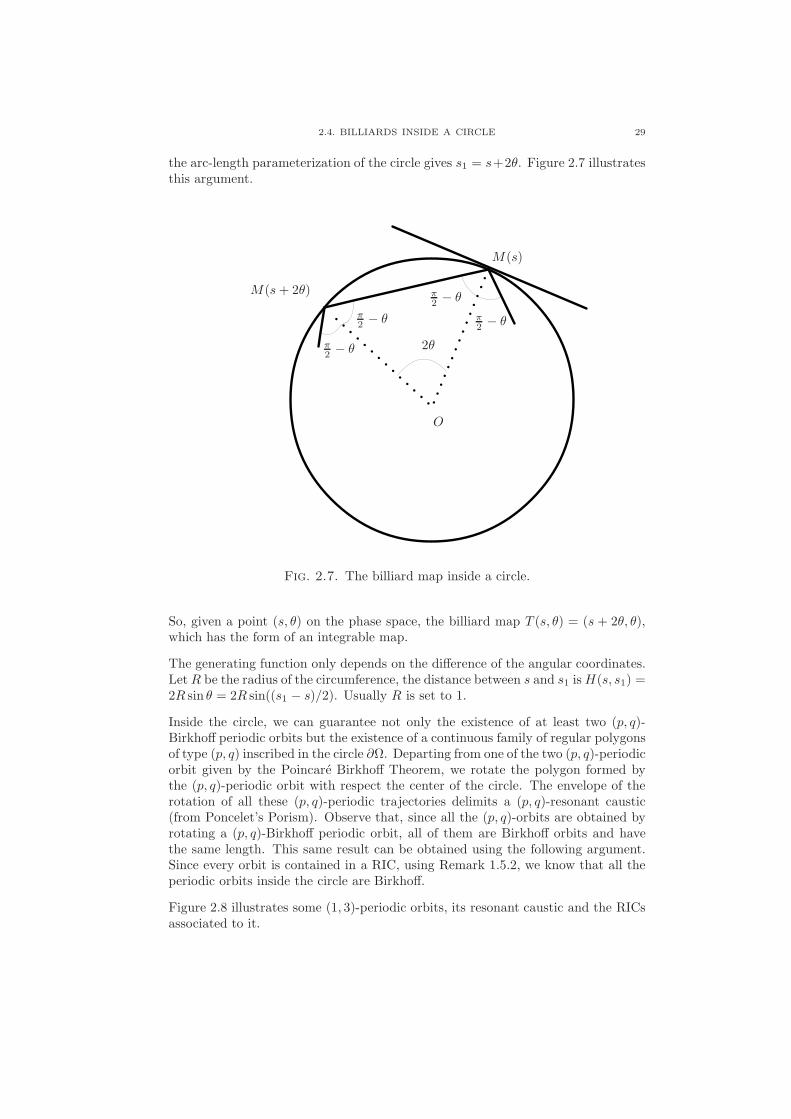
the arc-length parameterization of the circle gives s1 = s+2θ. Figure 2.7 illustratesthis argument.

π2 − θ

π2 − θ

π2 − θ

π2 − θ

2θ

M(s)

M(s+ 2θ)

O

Fig. 2.7. The billiard map inside a circle.

So, given a point (s, θ) on the phase space, the billiard map T (s, θ) = (s + 2θ, θ),which has the form of an integrable map.

The generating function only depends on the difference of the angular coordinates.LetR be the radius of the circumference, the distance between s and s1 isH(s, s1) =2R sin θ = 2R sin((s1 − s)/2). Usually R is set to 1.

Inside the circle, we can guarantee not only the existence of at least two (p, q)-Birkhoff periodic orbits but the existence of a continuous family of regular polygonsof type (p, q) inscribed in the circle ∂Ω. Departing from one of the two (p, q)-periodicorbit given by the Poincare Birkhoff Theorem, we rotate the polygon formed bythe (p, q)-periodic orbit with respect the center of the circle. The envelope of therotation of all these (p, q)-periodic trajectories delimits a (p, q)-resonant caustic(from Poncelet’s Porism). Observe that, since all the (p, q)-orbits are obtained byrotating a (p, q)-Birkhoff periodic orbit, all of them are Birkhoff orbits and havethe same length. This same result can be obtained using the following argument.Since every orbit is contained in a RIC, using Remark 1.5.2, we know that all theperiodic orbits inside the circle are Birkhoff.

Figure 2.8 illustrates some (1, 3)-periodic orbits, its resonant caustic and the RICsassociated to it.

30 2. BILLIARDS

2π

π

00

2π/3

π/3

Fig. 2.8. At left, some (1, 3)-periodic orbits. All the trajectorieshave the same incidence angle θ at each impact point. The mapis integrable and the resonant RICs are θ = constant on the phasespace, in particular θ = π/3 when the trajectories are traveledcounterclockwise and θ = 2π/3 when they are traveled clockwise.

2.5. Elliptic billiards

Let ∂Ω be an ellipse. Without loss of generality, we can consider by a translationand a similarity that, in cartesian coordinates, the boundary can be expressed as

∂Ω =

(x, y) ∈ R2 :

x2

a2+

y2

b2= 1

,

with a > b > 0. Thus, the foci are located at (c, 0) and (−c, 0), where c2 = a2 − b2.

We will not be taking the arc-length parameter s to parameterize the boundary.Instead, we will be choosing the parameterization given byM(ϕ) = (a cosϕ, b sinϕ),which is the most natural way to parameterize an ellipse. Thus, the preservedmeasure is ||M ′(ϕ)|| sin θdϕdθ.

The elliptic billiard is not an integrable map as we have defined before but it isLiouville integrable.

Definition 2.5.1. Let T be an area-preserving map. If there exists a non-constantfunction I(ϕ, θ) : T × (0, π) → R such that it is a first integral (equivalently,I T = I) we say that T is Liouville integrable.

The first integral is λ2(ϕ, θ) = (a2− b2) sin2 ϕ− ||M ′(ϕ)||2 cos2 θ+ b2 (see [2]). Theexistence of a first integral implies that the phase space is foliated by invariantcurves, λ2 = constant. In particular, if the curve λ2 = constant is not contractibleto a point, we have found a RIC. Actually, from the symmetry of the problem, wehave found two RICs. The phase space foliated by curves λ2 = constant can beseen in Figure 2.9.

2.5. ELLIPTIC BILLIARDS 31

0 π 2π

a

b

−a

−b

Fig. 2.9. Portrait phase space of an elliptic billiard. Some curvescorresponding to λ2 = constant are shown. The coordinates usedon the phase space are (ϕ, r), where r = ||M ′(ϕ)|| cos θ. In thesecoordinates, the phase space looks simpler. However, the domainis not the whole annulus, but the region between the dashed lines.This figure has been taken from [2]; thanks to R. Ramırez-Ros andP. Sanchez Casas.

As we have seen in Section 2.3, where we have found a one-to-two correspondencebetween caustics and RICs, this foliation allows us to affirm that any trajectory suchthat 0 < λ2 < b2 has a convex caustic. Also, if this caustic has a rational rotationnumber p/q, we have found that it is resonant (as we already knew from Poncelet’sPorism). Recalling Remark 1.5.2, all these (p, q)-periodic orbits are Birkhoff.

It can be proved that any convex caustic Γ on the elliptic billiard is a confocalellipse to ∂Ω. Indeed, the convex caustics can be characterized by the first integralλ2. Given λ ∈ (0, b), the corresponding convex caustic is

Γ = Cλ =

(x, y) ∈ R2 :

x2

a2 − λ2+

y2

b2 − λ2= 1

.

Observe that for λ = 0 we obtain the boundary, C0 = ∂Ω, and the rotation num-ber is ρ = ρ(0) = 0. Instead, for λ = b the ellipse obtained is degenerate, it isthe segment linking the two foci. The trajectory is then the (1,2)-periodic orbitcorresponding to the diameter. Therefore, for λ = b, ρ(b) = 1/2. The rotationnumber is a monotonically increasing function and therefore, for any p, q ∈ N suchthat gcd(p, q) = 1 and p < q/2, there exists a convex (p, q)-resonant caustic.

Also, it can be proved that the trajectories such that b2 < λ2 < a2 are in corre-spondence with nonconvex caustics which are hyperbolas with the same foci as ∂Ω.From Poncelet’s Porism, we know that all the trajectories tangent to hyperbolaswith a rational rotation number, p/q, are (p, q)-periodic orbits. None of these peri-odic orbits are Birkhoff. However, by looking at the phase space we can find some

32 2. BILLIARDS

other coordinates with which these (p, q)-periodic orbits from resonant caustics areBirkhoff. To argue it, we prefer to first introduce the following observations.

As we have seen in Section 2.2.5, on any strictly convex billiard, we can assure thatat least one (1, 2)-periodic orbit is hyperbolic, the one associated to the diameter.The (1, 2)-periodic orbit related to the width of the ellipse has impact points onthe boundary (0, b) and (0,−b). Therefore the chord length is 2b. Using the pa-rameterization given at this section, the two points correspond to impact pointsϕ = π/2 and ϕ = 3π/2 respectively and the curvature obtained at each impactpoint is κ(π/2) = κ(3π/2) = b/a2. Thus, 2b(b/a2 + b/a2) = 4b2/a2 < 4 and this(1, 2)-periodic orbit is elliptic, see condition (12).

Now, we justify which coordinates choose so that periodic orbits on contractibleinvariant curves become Birkhoff. We pick an easy example. Consider the (2, 4)-orbit on Figure 2.10. Taking a look to the phase space, we see that the angularcoordinates do not behave as a rigid rotation on the circle. However, if by symmetrywe move the two iterates of the orbits that make turns to the second elliptic point,p2 and p4, to the first one becoming p′2 and p′4, we see that the four iterates actlike a rigid rotation around the first elliptic point. This idea can be rigorouslyformalized using the Birkhoff normal form presented in Section 3.1 below.

2.5. ELLIPTIC BILLIARDS 33

p1 p3

p2

p4

p′2

p′4

0 π 2π

a

b

−a

−b

Fig. 2.10. The non-Birkhoff (2, 4)-periodic orbit is said to be a(1, 4)-Birkhoff when looking at the rotation around one of the twoelliptic fixed points on the phase space.

Chapter 3

General tools

3.1. Birkhoff normal form

Normal forms theory consists on writing a map near an invariant object in somenew coordinates such that the expression for the map in these new coordinates issimpler. One possible way to achieve this simpler form is by means of a sequenceof changes of coordinates, each one of them cancelling some terms in the expansonsof the map. This procedure does not need to be convergent. Even if it is divergent,the knowledge of the normal form up to a certain finite order gives importantinformation about the qualitative behaviour of the map.

We will be restricting ourselves to the two dimensional case. Here we quote someresults in [25, §23].

Let T : (x, y) 7→ (x1, y1) be an area-preserving analytic map defined near a fixedpoint which, without loss of generality, we will assume to be the origin. We will alsoassume that the linear terms have already been brought to a normal form. Thenour initial map has the following form,

x1 = T1(x, y) = λx+∑

k>1

T1k, y1 = T2(x, y) = µy +∑

k>1

T2k,(13)

where Tik are homogeneous polynomial in (x, y) of degree k, for i = 1, 2.

As we have seen in Subsection 2.2.5, according to Spec(DT (0)) = λ, µ, the origincan be classified as parabolic, as hyperbolic with or without reflection or as elliptic.Henceforth, we will not consider the parabolic case.

We want to determine a change of variables C : (ξ, η) 7→ (x, y) such that the map Tin the new coordinates, that is N := C−1TC, is as simple as possible. Since thelinear part of (13) is already in normal form, linear terms of the coordinate trans-formation correspond to the identity. Thus, we look for a nonlinear transformationof the form

x = C1(ξ, η) = ξ +∑

k>1

C1k, y = C2(ξ, η) = η +∑

k>1

C2k,(14)

with Cik homogeneous polynomial in (x, y) of degree k, for i = 1, 2.

35

36 3. GENERAL TOOLS

The simplest map we would like to achieve as normal form would be N(ξ, η) =(λξ, µη) which would imply to cancel all terms of order greater than one. Let ussee why this is not possible.

Relation N = C−1TC is equivalent to CN = TC and we can compare the coeffi-cients of the series. Observe that

CN = TC ⇔

C1(λξ, µη) = T1(C1(ξ, η), C2(ξ, η))C2(λξ, µη) = T2(C1(ξ, η), C2(ξ, η)).

(15)

It is easy too see that the linear terms coincide when inserting series from (13) and(14) into (15). Assume all the coefficients of all the terms of degree less than k agreein (15) and we have determined polynomials C1l and C2l for l < k. Equations (15)lead to

C1k(λξ, µη) = λC1k(ξ, η) + . . . , C2k(λξ, µη) = µC2k(ξ, η) + . . .(16)

where the terms not written down explicitly are homogeneous polynomials of de-gree k whose coefficients have already been determined. Writing C1k(ξ, η) =∑k

l=0 alξk−lηl and C2k(ξ, η) =

∑kl=0 blξ

k−lηl, we have

C1k(λξ, µη)− λC1k(ξ, η) =∑k

l=0 al(λk−lµl − λ)ξk−lηl

C2k(λξ, µη) − µC2k(ξ, η) =∑k

l=0 bl(λk−lµl − µ)ξk−lηl.

(17)

Using (17) into (16), one can see that coefficients al and bl can only be determinedif factors (λk−lµl − µ) and (λk−lµl − λ) are all different from 0.

Since our map T is area-preserving, we have relation λµ = 1 and therefore λl+1µl−λ = 0 and λlµl+1 − µ = 0 for any l. So it is clear we can not obtain a normal formas simple as we have proposed, N(ξ, η) = (λξ, µη).

The simplest expression we may achieve is a normal form of type

N(ξ, η) = (uξ, vη), u =∑

k≥0

α2k(ξη)k, v =

∑

k≥0

β2k(ξη)k.(18)

If λ is not a root of unity and the equations

∂ξC1 − ∂ηC2 = σ(ξ, η)∂ξC1∂ηC2 − ∂ξC2∂ηC1 − 1 = τ(ξ, η) − 1

(19)

are series not containing powers of ω = ξη alone, then, there exists a unique formalsubstitution C of type (14) that brings a map like (13) into the normal form (18).It is shown that C is then an area-preserving map and we also obtain the formalrelation uv = 1. Moreover, this last condition is not only necessary but also suf-ficient for (13) to be area-preserving. From this condition, one can observe thatξ1η1 = ξη and therefore the product ξη is a first integral.

With some additional hypotheses, the normal form can still be reduced a little bitmore. We assume the initial map (13) real and, again, λ is not a root of the unity.

If the origin is a hyperbolic point without reflection, there exists a unique real powerseries,

w =

∞∑

k=0

γk(ξη)k, γ0 such that λ = eγ0 ,(20)

3.2. MOSER’S TWIST THEOREM 37

such that u = ew, v = e−w, and the normal form becomes

ξ1 = ewξ, η1 = e−wη.

If the origin is a hyperbolic point with reflection, there exists a unique real powerseries w of the same form of equation (20) such that u = −ew, v = −e−w, and thenormal form becomes

ξ1 = −ewξ, η1 = −e−wη.

For the elliptic case we can also find a unique real power series w of the same formas the hyperbolic case (20) but with γ0 ∈ (−π, π) such that λ = eiγ0 and such thatu = eiw, v = e−iw, and the normal form is then

ξ1 = eiwξ, η1 = e−iwη.

To express this normal form in terms of real variables, we can apply the followinglinear transformation

ξ = r + is, η = r − is, ξ1 = r1 + is1, η1 = r1 − is1

and finally obtain

r1 = r cosw − s sinw, s1 = r sinw + s cosw, w =

∞∑

k=0

γk(r2 + s2)k,(21)

where γk, k ≥ 0, are the Birkhoff coefficients.

If there exists a non-zero Birkhoff coefficient, this normal form is an integrable twistmap, as we see at Subsection 3.2.1.

Relaxing conditions, particularly, requiring that ∂ξC1 − 1 and ∂ηC2 − 1 do notcontain powers of ω = ξη instead of asking for equations (19) to not be seriescontaining powers of ω = ξη alone, we find a unique substitution C which is nolonger area-preserving.

Once the series are computed in a formal sense, one can look for convergence of theseseries. It can be shown that in the hyperbolic case the series C1(ξ, η) and C2(ξ, η)converge in some neighbourhood of the origin. In the elliptic case, in general onehas divergence. It can be shown that in some cases convergence can occur but thereis no general method to determine whether there exists convergence or divergence.

3.2. Moser’s Twist Theorem

Moser’s Twist Theorem belongs to the KAM (Kolmogorov-Arnol’d-Moser) theory.This theory is the most efficient tool when dealing with RICs with “very irrational”rotation numbers, which, as we will see, are defined more precisely as Diophantinenumbers. Here, we will obtain RICs on a perturbative setting of an initially inte-grable area-preserving twist map.

Let T be an integrable area-preserving twist map

T : T× [a0, b0] → T× [a0, b0]

(s, r) 7→ (s+ α(r), r)

38 3. GENERAL TOOLS

twisting to the right, that is α′(r) > 0 for all r ∈ [a0, b0]. Observe that every circleT × r is a RIC. We want to study what happens to the RICs if we add someperturbative terms to T . Precisely, we want to prove the existence of infinitelymany RICs.

Consider A : (s, r) 7→ (s+ α(r) + f(s, r), r + g(s, r)), with f, g small perturbations.Consider f, g, α real analytic functions, 2π-periodic in s. In order to ensure theexistence of a RIC, the smallness condition in f and g is not sufficient. For example,consider g ≡ δ, δ small but constant, then r will increase monotonically and neverclose. A sufficient hypothesis to ensure this existence is the intersection property.

Definition 3.2.1. The map A satisfies the intersection property if for any Γ :=graphv, with v : s 7→ γ(s), Γ intersects its image, Γ ∩ A(Γ) 6= ∅.

Before stating the theorem, we simplify the setting. Consider the change of variables(s, r) 7→ (x, y) = (s, α(r)/γ), with γ = |α(b0) − α(a0)|. In the new variables, themap is

x1 = x+ γy + f(x, y),y1 = y + g(x, y),

(22)

where f and g still real analytic and 2π-periodic with respect to x.

Observe y ∈ [α(a0)/γ, α(b0)/γ] = [a, b], which is an interval of length 1. We canimpose, restricting ourselves to a narrower annulus, γ ≤ 1.

Since f , g are real analytic functions, they can be extended to a complex domainof the form D = (x, y) ∈ C2, |ℑx| < r0, y ∈ D′, where D′ is a complex neigh-bourhood of [a, b]. We may take 0 < r0 ≤ 1. Finally, we will assume that map Asatisfies the intersection property.

Definition 3.2.2. Given c0 > 0 and µ > 2, let

(23) D(c0, µ) :=

ω ∈ R :

∣∣∣ωq2π

− p∣∣∣ < c0

qµ, ∀p ∈ Z, q ∈ N

and D(µ) := ∪c0>0D(c0, µ). The numbers ω ∈ D(µ) are called Diophantine.

Observe that the Diophantine condition on (23) implies that ω is sufficiently awayof any rational number p/q. The set D(µ) has full measure in R for any µ > 2.Further information on Diophantine numbers can be found in [20, §III. A] or [4].Theorem 3.2.1 (Moser’s Twist Theorem, [25]). Under these hypotheses, for anyε > 0 there exists δ = δ(ε,D) > 0, δ not depending on γ, such that for |f |+ |g| ≤ γδin D, the map A has a RIC that can be parameterized as

x = ξ + u(ξ)y = v(ξ)

with u, v real analytic and 2π-periodic in ξ, |ℑξ| < r0/2

and such that the restriction of the application to the curve is the translation ξ 7→ξ + ω for some Diophantine rotation number ω. Also, functions u and v satisfy

|u|+ |v − γ−1ω| < ε.

In fact, there exists a RIC with rotation number ω for any ω ∈ D(c0, µ) ∩ [γ(a +s0), γ(b− s0)], for some c0 > 0, 0 < s0 < 1/4 and µ > 2.

3.2. MOSER’S TWIST THEOREM 39

The invariant curve found is related to the initial invariant curve of the integrablemap with a rotation number ω. Since ω is just chosen in order to satisfy theDiophantine condition (23), we can ensure that any RIC that has a Diophantinerotation number persists.

3.2.1. Stability criterion for area-preserving maps around an elliptic

fixed point. We know that under suitable hypotheses on the eigenvalues, wecan express an area-preserving map near an elliptic fixed point in Birkhoff co-ordinates (21) as

u1 = u cosw − v sinw +O2l+2

v1 = u sinw + v cosw +O2l+2,(24)

where w = γ0 + γl(u2 + v2)l, γl is the first non-zero Birkhoff coefficient of the

Birkhoff normal form, γl > 0, l > 0 and O2l+2 represents a power series in u and vcontaining terms of order greater or equal that 2l+ 2.

We will show that for any 0 < ε < ε0, with ε0 sufficiently small, the disk D =(u, v) s.t. u2 + v2 < ε2 contains an invariant curve surrounding (u, v) = 0. Thiscurve acts as a barrier for the dynamics and therefore we can deduce that theelliptic point is stable.

If we introduce polar coordinates, θ and r, as

u = εr1/2l cos θ, v = εr1/2l sin θ,

then, the equations (24) turn into

εr1/2l1 cos θ1 = εr1/2l cos θ cosw − εr1/2l sin θ sinw +O2l+2

εr1/2l1 sin θ1 = εr1/2l cos θ sinw + εr1/2l sin θ cosw +O2l+2,

which we can rewrite, using trigonometric relations, in coordinates (θ, r) as

θ1 = θ + w +O2l+1

r1 = r +O2l+1,

Taking into account w = γ0 + γl(u2 + v2)l = γ0 + γlε

2lr, we can still do anotherchange of variables, considering x = θ and r = y + γ0/(γlε

2l) and we get thefollowing map,

x1 = x+ γy + f(x, y)y1 = y + g(x, y),

(25)

where γ = γlε2l and f(x, y) and g(x, y) contain the terms in ε.

It is clear that we can apply Moser’s Twist Theorem to map (25). The functions fand g are real analytic and therefore can be extended to a complex domain. Also,the variable x is 2π periodic and we can consider 0 < y < 1. The intersectionproperty is easily deduced from the area-preserving property. Last condition to bechecked is |f |+ |g| < γδ(ε) and we have

|f |+ |g|γ

=O(ε2l+1)

γlε2l= O(ε).

40 3. GENERAL TOOLS

The same ideas used in this example to find stability around an elliptic fixed pointare used by Kamphorst and Pinto-de-Carvalho in [21]. There, for strictly convexbilliards, the stability of the elliptic (1,2)-periodic orbits is studied by explicitlycomputing the first Birkhoff coefficient. It only depends on the first derivatives ofthe curvature of the boundary at the impact points of the (1,2)-periodic orbits andalso the distance between them. Then, for a given strictly convex billiard, if thefirst Birkhoff coefficient is nonzero, one can assure stability of the (1,2)-periodicelliptic orbit.

3.3. Melnikov potential for perturbations of area-

preserving twist maps

Moser’s Twist Theorem requires Diophantine rotation numbers for the invariantcurves. If we have a resonant curve, it will be eventually destroyed under pertur-bation. The tool used to study the perturbed map is the Melnikov potential.

Melnikov methods are commonly used for computing the splitting of separatricesin maps and flows (see Section 4.1). A less common application of the Melnikovmethod is the one used for studying the perturbation on the surroundings of aresonant curve of an integrable twist map. This is the one we present in thissection. The geometric idea behind this method can be found in [6, §VI.] and [5,§20], and it was developed and used at [24] and [22].

Let T : T×[0, π] → T×[0, π] be an area-preserving twist map. Let H be its generat-

ing function. Consider Υ(p,q)0 a (p, q)-resonant RIC. By the Birkhoff Theorem 1.2.1,

Υ(p,q)0 = graphv := (s, v(s)), s ∈ R/ℓZ.

Consider Tε = T + O(ε) to be a perturbation of the area-preserving twist map T

and Tε to be its lift. Finally, let Hε = H + εH1 +O(ε2) be the perturbation on thegenerating function.

There exists a couple of radial curves, Υε = graph vε and Υ ∗ε = graph v∗ε close to

the initial curve, Υ(p,q)0 , such that the first graph is vertically projected onto the

second one after q iterations of map Tε.

Lemma 3.3.1 ([22]). There exist a constant η > 0 and two smooth functions vε, v∗ε :

T → [0, π] defined for ε ∈ (−ε0, ε0), ε0 > 0, such that

i. vε(s) = v(s) +O(ε) and v∗ε (s) = v(s) +O(ε), uniformly in s ∈ T;ii. T q

ε (s, vε(s)) = (s, v∗ε (s)) for all s ∈ T; and

iii. Υε = graph vε = (s, θ) : |θ − v(s)| < η and pr1Tqε (s, θ) = s + pℓ, where Υε

denotes the lift of Υε obtained when considering the lift vε of the function vεand pr1 is the projection onto the first coordinate, pr1 : R×(0, π) → R, (s, θ) 7→s.

From this result, one can easily extract the following conclusion.

3.3. MELNIKOV POTENTIAL FOR PERTURBATIONS OF AREA-PRESERVING TWIST MAPS41

Corollary 3.3.2 ([22]). The intersection of both radial curves contains all the

(p, q)-periodic orbits of Tε close to the former RIC Υ(p,q)0 . Also, the (p, q)-resonant

RIC persists if and only if both curves coincide everywhere.

Thus, we need to quantify the separation between graphs Υε and Υ ∗ε .

Lemma 3.3.3 ([22]). v∗ε (s) − vε(s) =(W

(p,q)ε

)′(s), where W

(p,q)ε : T → R is a

function whose lift is

W (p,q)ε =

q−1∑

j=0

Hε(sj(s, ε), sj+1(s, ε)), sj(s, ε) := T jε,1(s, vε(s)).

Corollary 3.3.4 ([22]). The unperturbed RIC persists if and only if(W

(p,q)ε

)′(s) ≡

0.

Definition 3.3.1. The subharmonic potential of the (p, q)-resonant RIC Υ(p,q)0 is

the function W(p,q)ε : T → R.

As any Melnikov method, it is usual to center the interest in the low order termsof the perturbative potential. Consider the expansion of the subharmonic function,

W(p,q)ε (s) = W

(p,q)0 (s) + εW

(p,q)1 (s) +O(ε2). The zero-order term of this expansion

vanishes since (W

(p,q)0

)′(s) = v∗0(s)− v0(s) = v(s) − v(s) ≡ 0.(26)

Definition 3.3.2. The first order term of the subharmonic potential, W(p,q)1 , is

called the subharmonic Melnikov potential of the (p, q)-resonant RIC Υ(p,q)0 for the

perturbation Tε.

The previous results lead to

Corollary 3.3.5 ([22]). If the subharmonic Melnikov potential is not constant,

then the (p, q)-resonant RIC Υ(p,q)0 does not persist under the perturbation Tε.

And finally, it can be proved that the subharmonic Melnikov potential can bedefined in a much simpler way.

Proposition 3.3.6 ([22]). The lift W(p,q)1 (s) is

W(p,q)1 (s) =

q−1∑

j=0

H1(sj , sj+1),(27)

where sj := T j(s, v(s)) and H(s, s1) = H0(s, s1) + εH1(s, s1) +O(ε2).

Chapter 4

Specific results of perturbative the-

ory

4.1. An example of exponentially small phenomena:

upper bound of the splitting of invariant curves

In this section we give a result on exponentially small bounds. The problem pre-sented is not directly related to the one we are interested in. Yet, since we willbe looking for exponentially small bounds, this example helps to understand thebehaviour of certain singular systems.

Before presenting the setting and results, we briefly introduce some basic definitions.Let T : U → U , U = U ⊂ R2, be an area-preserving diffeomorphism. An hyperbolicfixed point is also called a saddle point.

By the Hadamard-Perron Theorem [14, §6], a saddle point p0 has one-dimensionalstable and unstable manifolds, respectively, for δ sufficiently small,

W sloc(p0) := p ∈ U : ‖T n(p)− p0‖ < δ for n ≥ 0,

Wuloc(p0) := p ∈ U : ‖T n(p)− p0‖ < δ for n ≤ 0.

These local manifolds can be infinitely continued with the help of the iterates of Tgiving rise to the stable and unstable invariant manifolds

W s(p0) := p ∈ U : limn→∞

‖T n(p)− p0‖ = 0 =⋃

n∈Z

T n(W sloc(p0)),

Wu(p0) := p ∈ U : limn→∞

‖T n(p)− p0‖ = 0 =⋃

n∈Z

T n(Wuloc(p0)).

Each invariant manifold has two branches departing from (or arriving to) the saddlepoint. These branches depart from (or arrive to) the saddle point according to thedirection given by the eigenvectors related to the eigenvalues of the linearized systemaround the saddle point. It is clear that a branch from the stable invariant manifoldof a saddle point cannot intersect to another stable branch of the same saddle pointor another. The same is established for the unstable branches.

43

44 4. SPECIFIC RESULTS OF PERTURBATIVE THEORY

However, a stable branch can intersect with an unstable one. The points on theintersection are called homoclinic points when both branches correspond to theinvariant manifolds of the same saddle point or heteroclinic points otherwise. Itis clear that the orbits of homoclinic (heteroclinic) points contain only homoclinic(heteroclinic) points. Thus, we refer to them as homoclinic (heteroclinic) orbits.

If a branch of the unstable manifold coincides with a branch of the stable manifoldof the same saddle point, we say that this invariant curve is a separatrix, whichwe usually note by Γ. A separatrix has a fish-shape form since both backwardand forward iterates of any point in the separatrix tend to the saddle point. Theterm separatrix is due to the fact that dynamics inside and outside this fish-shapedinvariant curve have different behaviours.

Let Th : R2 → R2, h > 0, be an area-preserving map with a separatrix Γh to asaddle point p0. Suppose Spec(DTh(p0)) = e+h, e−h. Observe that this saddlepoint is weakly hyperbolic if h is small. Generically, the separatrix splits in atransverse way when introducing perturbations. Here, we consider a perturbationdepending on a parameter ε, Th,ε = Th +O(ε).

We proceed to measure the splitting using a Melnikov method. Suppose we are ableto compute the O(ε)-term of a certain splitting quantity S (for example, distancebetween the invariant manifolds), so that S = S(h, ε) = εS1(h) + O(ε2) for anyfixed h > 0. But, is it always the first term of this expansion the one dominating?What can we say about S when both h and ε are small? When h is no longer fixed,the first term may not be the most important. Then, Melnikov methods fail sinceone has to know the asymptotic behaviour of all the terms in the expansion (verydifficult) and not only the first ones. Thus, another approach has to be taken.

Next theorem gives an upper bound for the size of the splitting in a singular case.

Theorem 4.1.1 (Fontich-Simo, [11]). Let Fh : R2 → R2, h > 0, be a diffeomor-phism such that:

• Fh = Id+hF1 + hβF2, where F1 : R2 → R2, F2 : R2 × R+ → R2, β > 0 andF1(0, 0) = F2(0, 0, h) = (0, 0).

• SpecDFh(0, 0) = λ, λ−1, where λ = 1 + h+O(h2).• The system z′ = F1(z) has an homoclinic loop to the origin, γ(t).• Fh is analytic in a complex neighbourhood of γ(t), |ℑt| < d∗.

Then, for any d ∈ (0, d∗), there exists C > 0 such that the distance between theinvariant manifolds is less or equal than Ce−2πd/h as h tends to 0+.

4.2. Existence of caustics near the billiard bound-

ary

Next, we present a direct application of Moser’s Twist Theorem. This result goesback to Lazutkin [17].

4.2. EXISTENCE OF CAUSTICS NEAR THE BILLIARD BOUNDARY 45

If we recall the notation used in Section 2.3, a caustic Γ can be charaterized by theinvariant η, which is the rotation number of the diffeomorphism from Γ to itselfdefined by M 7→ M1, where M and M1 are the points on Γ that draw tangents toa point N on ∂Ω. We denote the caustic defined by the rotation number η as Γ(η).

Consider the Cantor set

D = Dη∗,c0,µ := (0, η∗) ∩ D(c0, µ),

where D(c0, µ) is the set of Diophantine numbers defined in (23), and η∗ ≪ 1. Notethat 0 ∈ D. Also recall that if a caustic Γ has a rotation number belonging tothis set, η(Γ) ∈ D, then the rotation number is poorly approximated by rationalnumbers.

Theorem 4.2.1 (Lazutkin, [17]). Let Ω be a sufficiently smooth and strictly con-vex billiard table. Then, there exists a Cantor family of smooth convex causticsΓηη∈D ∈ Ω, with limη→0+ Γη = ∂Ω, whose union has positive area.

Recalling the relations and notation between convex caustics and RICs seen atSection 2.3, the theorem can be reformulated as follows.

Theorem 4.2.2. The billiard map associated to a sufficiently smooth and strictlyconvex billiard table has two collections of RICs, Υ±

η η∈D ∈ T × (0, π), with

limη→0+ Υ−η = T × 0 and limη→0+ Υ+

η = T × π, whose union has positivearea.

Remark 4.2.1. After Douady, the minimum smoothness required is that the bound-ary ∂Ω is at least C6, [10].

To prove this result recall that the billiard map T can be extended to its boundary,where it becomes the identity map. Therefore, when θ tends to 0, the point (s, θ)tends to be stationary for all s. We want to find a family of invariant closed curvesnear this stationary curve which will be Υ−

η η∈D. The other family, Υ+η η∈D, is

directly obtained by the billiard symmetry.

First, we denote by ~x(s) the arc-length parameterization of ∂Ω, ~t(s) its tangent unit

vector and ~n(s) the unit normal vector, ~n(s) = ρ(s)~t′, ρ(s) the radius of curvatureof ∂Ω.

In a neighbourhood of the stationary curve θ = 0, we can write T as

(28)

s1 = s+ 2ρθ + (4/3)ρρ′θ2 +

((2/3)ρ2ρ′′ + (4/9)ρρ′2

)θ3 +O(θ4)

θ1 = θ − (2/3)ρ′θ2 +(−(2/3)ρρ′′ + (4/9)ρ′2

)θ3 +O(θ4),

where we have not explicitly written the dependence of the curvature radius on theparameter s, ρ = ρ(s). The explicit derivation of (28) is placed in Appendix A.

We can then introduce the coordinates ξ(s, θ) ∈ R/Z and η = η(s, θ) > 0 given by

ξ = C

∫ s

0

ρ−2/3(s)ds, η = 4Cρ1/3(s) sin(θ/2),

with C−1 =∫ L

0ρ−2/3(s)ds. These coordinates are well-defined for small incidence

angles θ. Observe that η(s, 0) ≡ 0 and also that 0 < θ ≪ 1 if and only if 0 < η ≪ 1.


In these new coordinates, for η sufficiently small, η < η∗, the billiard map becomes

ξ1 = ξ + η +O(η3) = ξ + η + η3f(ξ, η)η1 = η +O(η4) = η + η4g(ξ, η),

This setting is suitable to apply Moser’s Twist Theorem (recall Equation (22)).For f, g ≡ 0 all curves η = constant are invariant. For f, g small perturbations,if the intersection property holds, which it does because dm = constant |ξ|dξdηis preserved, the curves with η satisfying a Diophantine condition, that is η ∈ D,persist after the perturbation.

4.3. Break-up of caustics

In the previous section, we have given a criterion for the existence of caustics in theneighbourhod of the boundary ∂Ω. This criterion was based on a KAM theoremapplied on a neighbourhood of the stationary curve θ = 0. Hence, the obtainedcaustics have Diophantine rotation numbers.

Nevertheless, we are interested in periodic trajectories. When the envelope of aset of periodic trajectories defines a caustic, this caustic has a rational rotationnumber. Therefore, the previous theorem can not be used.

Let p, q ∈ N, gcd(p, q) = 1 and p < q/2. Recall, from Section 2.5, that elliptic bil-liards are Liouville integrable. Therefore any (p, q)-periodic orbit is on an invariantcurve. Following Poncelet’s Porism, these curves are foliated by (p, q)-periodic or-bits. The invariant curves not contractible to a point (the RICs) are in two-to-onecorrespondence with the resonant convex caustics, which are confocal ellipses tothe billiard boundary.

The results we will give refer to circular and elliptic billiards. We will see that,contrary to the RICs with Diophantine rotation numbers, the RICs with rationalrotation numbers do not persist under generic perturbations and therefore the reso-nant caustics are destroyed too. Recall that there will be at least two (p, q)-periodicorbits after the perturbation but the resonant caustic structure will not persist.

First we state a result focused on circular billiards. To introduce it, we need somenotation.

Consider, with out loss of generality, that the circle is centered at the origin andhas radius r0. We parameterize the circular table by M0 : T → ∂Ω ∈ R2, s 7→ r0~ns,where ~ns = (cos s, sin s).

We consider the generic perturbation Mε : T → ∂Ωε, s 7→ rε(s)~ns, where

rε(s) = r0 + εr1(s) +O(ε2).

Theorem 4.3.1 ([24]). Let∑

j∈Zrj1e

i js be the Fourier expansion of r1(s). Let

p and q be any integers, with p < q/2 and gcd(p, q) = 1. If there exists somej ∈ qZ\0, the (p, q)-resonant caustic does not persist under this perturbation.

4.4. LENGTH SPECTRUM OF CONVEX DOMAINS 47

The following result refers to elliptic billiards. As we have seen in Section 2.5, weparameterize the unperturbed elliptic boundary by M0 : (ϕ) = (c coshµ0 cosϕ, y =

c sinhµ0 sinϕ), c =√a2 − b2 and µ0 is such that a = c coshµ0 and b = c sinhµ0.

The advantage of this parameterization is that if we consider coordinates (µ, ϕ)instead of only ϕ we can parameterize any conic with the same foci than ∂Ω. Anyconfocal ellipse is determine by µ = constant while we can consider any hyperbolaby making ϕ = constant. As told, µ = µ0 parameterizes ∂Ω.

The perturbation ∂Ωε considered is similar to the one considered in the circularbilliard. The perturbation affects to µ0. Instead of being constant, it is substitutedby a smooth function µε(ϕ) = µ0 + εµ1(ϕ) + O(ε2). Hence, the parameterizationis Mε(ϕ) = (c cosh(µε(ϕ)) cosϕ, c sinh(µε(ϕ)) sinϕ).

Theorem 4.3.2 ([22]). Let µ1(ϕ) be a 2π-periodic entire function. If µ1(ϕ) isnot constant (respectively, µ1(ϕ) is not π-antiperiodic), then none of the convex(p, q)-resonant caustic ellipses with odd q (respectively, even q) persist under theperturbation µε(ϕ).

Both theorems rely on the study of the Melnikov potential for these perturbations.

4.4. Length spectrum of convex domains

Consider p, q ∈ Z, gcd(p, q) = 1, p ≤ q/2. Let Γ(p,q) be the set of all the (p, q)-orbitsat Ω. Let L(p,q) be the set of lengths of the orbits on Γ(p,q).

Definition 4.4.1. The set of numbers L = ℓN ∪ ⋃(p,q) L(p,q) is called the length

spectrum of the domain Ω.

We also denote by L(p,q) = supL(p,q) and l(p,q) = inf L(p,q). Finally, ∆(p,q) willdenote the difference on these two quantities, ∆(p,q) = L(p,q) − l(p,q).

In our work, we want to study the asymptotic behaviour of these three quantities.In this field, two results are worth to be mentioned. The first one deals with orbitswith a fixed number of turns inside ∂Ω, this is a fixed p, and with a large period, q.

Theorem 4.4.1 (Marvizi and Melrose, [18]). If the billiard table Ω is smooth andstrictly convex, then

(1) There exist coefficients cp,j such that

L(p,q), l(p,q) ≍ cp,0 +∑

j≥1

cp,jq−2j as q → ∞.

Coefficient cp,0 = pℓ and coefficient cp,1 is always negative.(2) There exist some “universal” functions gj : R

+ × Rj−1 such that

cj := c1,j =

∫ ℓ

0

gj

(κ(s), κ′′(s), . . . , κ(2j−2)(s)

), j ≥ 1,

where κ(s) is the curvature of ∂Ω parameterized by the arc-length parameter.(3) limq→∞ qk∆(p,q) = 0 for all k > 0. Equivalently, ∆(p,q) = O (q−∞).


The next result is valid for (p, q)-periodic orbits close to the (1,2)-periodic ellipticorbit on a billiard table with axial symmetries. We give the asymptotic behaviourof these orbits as p/q tends to 1/2. Recall that the definition of an elliptic periodicorbit has been given at Subsection 2.2.5.

Theorem 4.4.2 (Colin de Verdiere, [8]). Let Ω be a smooth convex domain of R2,symmetric with regard to both axis of coordinates. Assume that its shortest (1, 2)-periodic billiard trajectory is elliptic and ∂Ω is strictly convex at its endpoints.Consider in Γ(p,q) only the subset of (p, q)-periodic orbits which are close to the(1, 2)-periodic elliptic orbit. From this subset, we redefine L(p,q), l(p,q), L(p,q) and∆(p,q) as before. Then,

∆(p,q) = O(q−∞) as p/q → 1/2.

This theorem is obtained through the study of the Birkhoff normal form of the bil-liard map around its (1, 2)-periodic orbit. The non-resonance condition is necessaryto compute this normal form up to an arbitrary order.

Part 2

Goals and first results

Chapter 5

Discussion of problems to treat

5.1. Introduction to the problems

In Dynamical Systems, and more concretely, in the analytic context, the followingprinciple is generally assumed. Consider a quantity ∆ which tends asymptoticallyto zero as a certain parameter, q, tends to infinity and its asymptotic behaviouris faster than any order, that is ∆ = O(q−∞). Then, quantity ∆ is exponentiallysmall in parameter q.

This principle is not proved in general but we have already given an example inSection 4.1 where it applies: the distance between manifolds of close to the identityarea-preserving analytic maps is exponentially small in the characteristic exponent.

We have seen the results by Marvizi and Melrose and by Colin de Verdiere onthe length spectrum which predicted an asymptotic behaviour beyond all orders indifferent cases. We recall the notation and the results found.

Consider p, q ∈ N, gcd(p, q) = 1, p ≤ q/2. Let Γ(p,q) be the set of all the (p, q)-orbitsat the convex domain Ω. Let L(p,q) be the set of lengths of the orbits on Γ(p,q).The length spectrum of the domain Ω is L = ℓN ∪⋃(p,q) L(p,q) and the difference

between the maximum and the minimum length among the orbits on the set Γ(p,q)

is denoted by ∆(p,q).

On the one hand, the set Γ(1,q) approaches to the billiard boundary as q tends toinfinity. According to Marvizi and Melrose [18], ∆(1,q) turns out to be of orderO(q−∞).

On the other hand, consider only the (p, q)-periodic trajectories close to the (1, 2)-periodic elliptic orbits in billiards which are symmetric with respect to the widthand diameter. Then, Colin de Verdiere [8] found out that the same result holds,∆(p,q) = O(q−∞).

These results, together with the assumption of the principle mentioned above, leadus to search for exponentially small asymptotic behaviours of the difference oflengths among the set of (p, q)-periodic orbits under certain settings (for examplethe setting given by Marvizi and Melrose or the one by Colin de Verdiere).

51

52 5. DISCUSSION OF PROBLEMS TO TREAT

Yet, there exists another setting where to look for an exponential smallness of thedifference on the lengths of the (p, q)-periodic orbits of a billiard.

Consider an elliptic or circular billiard. We have seen that the billiard maps onthese type of billiards are Liouville integrable and the trajectories are contained ininvariant curves. We center ourselves on those curves which are RICs. Recall that,at a circular billiard, all the invariant curves are RICs while at an elliptic billiard,RICs are associated to convex caustics.

The billiard map can be restricted to each RIC and a rotation number can be as-signed to each RIC. Applying KAM theory to those RICs with Diophantine rotationnumbers, we know that the RICs will persist under small perturbations and, thus,their caustics will persist too.

Typically, as we have seen in Section 4.3, RICs with a rational rotation number p/qwill break down making the (p, q)-resonant caustic disappear. Although we will nothave a continuous family of (p, q)-periodic orbits after the perturbation, accordingto Poincare-Birkhoff Theorem, there will exist at least two (p, q)-periodic orbits.However, we will no longer be able to guarantee that ∆(p,q) = 0 on the set ofpersisting (p, q)-periodic orbits.

In analogy to Greene’s criterion [12], we believe that the difference ∆(p,q) tendexponentially to zero as p/q tends to the Diophantine rotation number of a RIC.Similar problems are studied in [9, Theorem 1.6].

5.2. Our approach

The subject presented is quite large and goes beyond the scope of a Master Thesis.In this work, we have just initiated the computations on the asymptotic behaviourof ∆(p,q) in some particular cases which we detail below.

We are interested in measuring the behaviour among all the elements on L(p,q) and,more concretely, in finding the asymptotic growth or order for the function ∆(p,q) asp/q tends to some specific rotation number whether it is 0 and we are approachingto the billiard boundary or it is an irrational number.

We take a look to Liouville integrable billiards, circular and elliptic billiards. Con-sider p, q ∈ N, p < q/2, and gcd(p, q) = 1, there always exists a (p, q)-resonantcaustic in correspondence to a RIC with rotation number p/q and its symmetric, aRIC with rotation (q − p)/p.

Henceforth, we slightly modify definitions on Γ(p,q), so that the only (p, q)-periodicorbits considered on the set Γ(p,q) are the ones tangent to a convex caustic, leavingthe (p, q)-periodic trajectories tangent to hyperbolas apart.

Recalling that the generating function of a billiard map is the length between twopoints on the billiard boundary, we can observe that the length of a (p, q)-trajectorycoincides with the definition of the subharmonic potential of the (p, q)-resonant RIC

5.2. OUR APPROACH 53

defined in Section 3.3. Thus,

∆(p,q) = maxW (p,q)ε (s) : s ∈ T −minW (p,q)

ε (s) : s ∈ T.We write the subharmonic potential as an expansion on the perturbation parameter:

W (p,q)ε (s) = W

(p,q)0 (s) + εW

(p,q)1 (s) +O(ε2).

Since the term W(p,q)0 (s) is also constant with respect to variable s (see equa-

tion (26)), we can write the difference ∆(p,q) as

∆(p,q) = ε∆(p,q)1 +O(ε2),

where ∆(p,q)1 := maxTW

(p,q)1 −minTW

(p,q)1 .

As it is usual with Melnikov methods, we will study first the behaviour of the loworder terms. Just as we discussed in Section 4.1, if q is not a fixed value, the loworder terms of this expansion may not be the dominant ones. Thus, if we wantto find asymptotic results on ∆(p,q) as p/q tends to a concrete number rotationnumber, we can not ignore the higher order terms of the expansion. Therefore, to

find an exponentially small bound, we have to deal with all the terms ∆(p,q)j for all

j > 0.

Despite this observation, our approach is focused on the Melnikov prediction for

the first order term, ∆(p,q)1 on circular and elliptic billiards.

We present the results in the next chapter.

Chapter 6

First results

6.1. Circular tables

We consider a circular billiard table, with boundary ∂Ω. Without loss of generality,we can assume

∂Ω :=(x, y) ∈ R2 : x2 + y2 = 1

.

As we have seen in Section 2.4, the billiard map is defined as T : T × [0, π] →T× [0, π], (s, θ) 7→ (s+2θ, θ), which is an integrable twist map. Therefore, followingSection 1.1, for all p, q ∈ N, p < q/2, the (p, q)-periodic orbits are set on a RICfoliated by (p, q)-periodic orbits. Geometrically, given any regular (p, q)-polygoninscribed in the circle, we obtain the rest of (p, q)-periodic orbits by rotating itwith respect to the origin. Thus, ∆(p,q) = 0.

Our aim is to measure the behaviour on the lengths among all these (p, q)-periodicorbits on a perturbed circular table, ∂Ωε. We want to study the difference of lengths

among Γ(p,q), that is ∆(p,q). In particular, we will study the first order term, ∆(p,q)1 .

We parameterize the circular boundary by the arc-length parameter, that is M0 :T → ∂Ω, s 7→ ~ns := (cos s, sin s). The generic perturbation we consider is theone already considered in Section 4.3. The perturbative parameter ε affects tothe distance to the origin at each direction. The perturbed circular boundary isdescribed as follows

Mε : T → ∂Ωε

s 7→ rε(s)~ns = (rε(s) cos s, rε(s) sin s),(29)

where rε(s) = 1 + εr1(s) +O(ε2).

As we have seen in Section 3.3, the subharmonic Melnikov potential can be com-puted as

W(p,q)1 (s) =

q−1∑

j=0

H1(sj , sj+1),

where sj is the first coordinate at the j-th iteration of the unperturbed billiard map

T at a point (s, v(s)) on the RIC Υ (p,q) = graphv with rotation number p/q.

55

56 6. FIRST RESULTS

From the study of the subharmonic Melnikov potential for the circular table and thegeneric perturbations introduced above, and as it is computed in [24], the previousformula for the subharmonic Melnikov potential can be written as

W(p,q)1 (s) = 2 sin(πp/q)

q−1∑

k=0

r1(s+ 2πkp/q) = 2q sin(πp/q)∑

j∈qZ

rj1ei js,(30)

where rj1 are the Fourier coefficients for function r1(s). That is, r1(s) =∑

j∈Zrj1e

i js.

Now, we can state an exponentially small upper bound for

∆(p,q)1 = max

T

W(p,q)1 −min

T

W(p,q)1 .

Proposition 6.1.1. Let r1(s) be a 2π-periodic analytic function in the strip S =s ∈ C : |ℑs| < ρ, for some ρ > 0. Given any ρ′ ∈ (0, ρ), there exists a constant

C = C(ρ′) such that ∆(p,q)1 ≤ Ce−ρ′q, if q ≫ 1.

Proof. From equation (30) we obtain that W(p,q)1 is 2π/q-periodic. Thus, we can

write W(p,q)1 (s) as its expansion in Fourier series,

W(p,q)1 (s) =

∞∑

n=−∞

cneinqs,

where

cn =q

2π

∫ 2π/q

0

W(p,q)1 (t)e−inqtdt.

The constant term c0 does not affect ∆(p,q)1 . Thus, we want to find an exponentially

small upper bound for the coefficients cn with n 6= 0.

Since r1 (s+ 2πk/q) is analytic in |ℑs| < ρ, for any k ∈ Z, so is W(p,q)1 (s). Note

that W(p,q)1 (s) is bounded on any imaginary strip |ℑs| ≤ ρ′ < ρ.

Then for any closed path γ in the strip |ℑs| < ρ, we have∫

γ

W(p,q)1 (t)e−inqtdt = 0.

To calculate cn, n < 0, consider the rectangle with vertices 0, 2π/q, i ρ′+2π/q, andi ρ′, with ρ′ < ρ. We then have

0 =

(∫ 2π/q

0

+

∫ i ρ′+2π/q

2π/q

+

∫ i ρ′

i ρ′+2π/q

+

∫ 0

i ρ′

)W

(p,q)1 (t)e−inqtdt.

By periodicity, the second integral cancels with the fourth. Then the first integralequals to the opposite of the third one. Thus,

2π

qcn =

∫ i ρ′+2π/q

i ρ′

W(p,q)1 (t)e−inqtdt

=

∫ 2π/q

0

W(p,q)1 (x+ i ρ′)e−inqxenρ

′qdx.

6.1. CIRCULAR TABLES 57

From equation (30),

max|ℑs|≤ρ′

|W (p,q)1 (s)| ≤ 2q sin(2πp/q) max

|ℑs|≤ρ′

|r1|.

Since the factor q sin(2πp/q) is bounded as q tends to infinity, we can find an upper

bound Kρ′ not depending on q. Thus, max|ℑs|≤ρ′ |W (p,q)1 (s)| < Kρ′ for q ≫ 1.

Hence, we obtain, for n < 0,

cn <q

2πe−|n|ρ′q

∫ 2π/q

0

Kρ′ · 1dt = Kρ′e−|n|ρ′q.

In fact, the same bound can be obtained for cn, n > 0, by taking the rectangle withvertices 0, 2π/q, −i ρ′ + 2π/q and −i ρ′.

Taking back the expression for W(p,q)1 (s), we have, for all s ∈ R,

∣∣∣W (p,q)1 (s)− c0

∣∣∣ =

∣∣∣∣∣∣∑

n6=0

cneinqs

∣∣∣∣∣∣≤∑

n>0

2Kρ′e−nρ′q

≤ 2Kρ′

e−ρ′q

1− e−ρ′q≤ 4Kρ′e−ρ′q,

where the last inequality is true by taking q such that ρ′q > ln 2.

Finally,

∆(p,q)1 = max

T

W(p,q)1 −min

T

W(p,q)1 ≤

∣∣∣maxT

W(p,q)1 − c0

∣∣∣+∣∣∣c0 −min

T

W(p,q)1

∣∣∣

≤ 8Kρ′e−ρ′q = Ce−ρ′q,

where C = 8Kρ′ . ⊓⊔

With this proposition, we have guaranteed that ∆(p,q)1 is exponentially small for

perturbations of the circular billiard of the form (29). In the next proposition, wegive an example of perturbations for which the same exponentially small behaviourholds as a lower bound.

Proposition 6.1.2. Let W(p,q)1 (s) = 2q sin(πp/q)

∑j∈qZ r

j1e

i js, where there exist

α, α ∈ R+ and m ∈ N such that

α|j|me−|j|ρ ≤ |rj1| ≤ α|j|me−|j|ρ, ∀j ∈ Z.

Then, ∆(p,q)1 ≥ Kqme−ρq, for some K ∈ R+.

Proof. Since r1(s) is real analytic, its Fourier coefficients verify that r−j1 = rj1 for

any j ∈ Z, where rj1 denotes the conjugate of the coefficient rj1.

Writing rj1 = aj1 + i bj1, with aj1, bj1 ∈ R, we have

W(p,q)1 (s) = 2q sin(πp/q)

∑

j∈qZ

(aj1 + i bj1)ei js

= 2q sin(πp/q)

a01 + 2aq1 cos(qs)− 2bq1 sin(qs) +

∑

|j|>q,j∈qZ

rj1ei js

.

58 6. FIRST RESULTS

We are now going to find an upper bound for∑

|j|>q,j∈qZ rj1e

i js. From the hypothe-

ses of the proposition, we have∣∣∣∣∣∣∑

|j|>q,j∈qZ

rj1ei js

∣∣∣∣∣∣≤ α

∑

|j|>q,j∈qZ

|j|me−|j|ρ|ei js| ≤ 2qmα∑

j≥2

jme−jρq.

Consider the function f(x) = xme−xρq. It tends to zero as x tends to infinity,f(0) = 0 and it is positive for x positive. Its unique maximum on R+ is at x∗ =m/(ρq). Then,

∣∣∣∣∣∣∑

|j|>q,j∈qZ

rj1ei js

∣∣∣∣∣∣≤ 2qmα

(f(max2, x∗) +

∫ ∞

2

f(x)dx

).

On the one hand,

f(max2, x∗) =

2me−2ρq if 2ρq ≥ m(m/(ρq))

me−m if 2ρq < m.

(31)

Observe that, since m and ρ are initially fixed, for q sufficiently large, we have

f(max2, x∗) = f(2) = O(e−2ρq).

On the other hand, ∫ ∞

2

f(x)dx =

∫ ∞

2

xme−xρqdx.

If we use the upper incomplete Gamma function, Γ(s, x) =∫∞

xts−1e−tdt, we obtain

∫ ∞

2

xme−xρqdx = (ρq)−(m+1)

∫ ∞

2ρq

tme−tdt = (ρq)−(m+1)Γ(m+ 1, 2ρq).

Using [3, §6.5.32], we obtain∫ ∞

2

xme−ρqxdx ≍ 2me−2ρq/(ρq) = O(q−1e−2ρq), as q → ∞.

Therefore, for q sufficiently large, we are able to obtain∣∣∣∣∣∣∑

|j|>q,j∈qZ

rj1ei js

∣∣∣∣∣∣≤ O(qme−2ρq).

Up to now, we know that, for all s ∈ T,

W(p,q)1 (s) ≤ 2q sin(πp/q)

((aq0 + 2aq1 cos(qs)− 2bq1 sin(qs)

)+O(qme−2ρq)

).

Next, we want to find an exponentially small lower bound for ∆(p,q)1 . We define the

function

f(s1, s2) := W(p,q)1 (s1)−W

(p,q)1 (s2), s1, s2 ∈ T.

6.1. CIRCULAR TABLES 59

Hence, ∆(p,q)1 ≥ f(s1, s2) for all s1, s2 ∈ T. Let f(s1, s2) = 2q sin(πp/q) (g(s1, s2) + h(s1, s2)),

where

h(s1, s2) :=∑

|j|>q,j∈qZ

rj1(ei js1 − ei js2 ) = O(qme−2ρq),

g(s1, s2) := 2(aq1(cos(qs1)− cos(qs2))− bq1(sin(qs1)− sin(qs2))

).

From the formulae of the sum of cosinus and sinus we obtain that

g(s1, s2) = 4 |sin (q(s1 − s2)/2)|∣∣∣aq1 sin (q(s1 + s2)/2) + bq1 cos (q(s1 + s2)/2)

∣∣∣ .

Observe that there exist s11 and s12 such that∣∣sin

(q(s11 − s12)/2

)∣∣ = 1,∣∣cos

(q(s11 + s12)/2

)∣∣ = 1,∣∣sin

(q(s11 + s12)/2

)∣∣ = 0.

Then,

g(s11, s12) = 4|bq1|.

And there also exist s21 and s22 such that∣∣sin

(q(s21 − s22)/2

)∣∣ = 1,∣∣cos

(q(s21 + s22)/2

)∣∣ = 0,∣∣sin

(q(s21 + s22)/2

)∣∣ = 1.

Then,

g(s21, s22) = 4|aq1|.

Consider s∗, s∗ ∈ T such that g(s∗, s∗) ≥ g(s1, s2) for all s1, s2 ∈ T. Thus,

g(s∗, s∗) ≥ 4maxaq1, bq1. Since

maxaq1, bq1 ≥√(

(aq1)2 + (bq1)

2)/2 = |rq1 |/

√2 ≥ αqme−ρq/

√2,

we have

g(s∗, s∗) ≥ 2√2αqme−ρq = O(qme−ρq).

Thus, the term which dominates f(s1, s2) is g(s1, s2) and

∆(p,q)1 ≥ f(s∗, s∗) ≥ 4q sin(πp/q)αqme−ρq.

Finally, as q tends to infinity, πp/q tends to zero. Thus, we use inequality 2x/π ≤sinx for x ∈ [0, π/2] to find that 2p ≤ q sin(πp/q) for q large enough. The finallower bound for q ≫ 1 is

∆(p,q)1 ≥ Kqme−ρq, K := 8αp.

⊓⊔

The hypotheses required for the proposition are not as strict as one might think.For example, the Fourier coefficients of the function

r1(s) =1

1− 2µ cos s+ cos2 s, µ ∈ (0, 1),

are rj1 = µ|j|. Since µ ∈ (0, 1), we can write µ = e−ρ, for some ρ ∈ R+. Then,

α|j|me−|j|ρ ≤ rj1 ≤ α|j|me−|j|ρ, by taking m = 0 and α ≤ 1 ≤ α.

60 6. FIRST RESULTS

It is sufficient to take derivatives of the function above to obtain examples satisfyingthe bounds of Proposition 6.1.2 with m 6= 0. Indeed,

gm(s) :=dm

dsmr1(s) =

∑gjmei js, gjm = rj1|j|m.

Also, observe that since rj1 must be in a certain interval, slight perturbations onthe Fourier coefficients of functions satisfying the hypotheses still give rise to otherfunctions satisfying the hypotheses.

6.2. Elliptic tables

We consider the elliptic billiard table

∂Ω := C0 =

(x, y) ∈ R2 :

x2

a2+

y2

b2= 1

, a > b > 0.

For all p, q ∈ N, p < q/2, the (p, q)-periodic orbits set on a RIC give rise to thesame (p, q)-resonant convex caustic. This convex caustic is a confocal ellipse whichcan be expressed as

Cλ =

(x, y) ∈ R2 :

x2

a2 − λ2+

y2

b2 − λ2= 1

for some 0 < λ < b. The parameter λ has a one-to-one correspondence withthe rotation number ρ. From Poncelet’s Porism, we know that all (p, q)-periodictrajectories have the same length.

Our aim is to measure the behaviour of the lengths of these (p, q)-periodic or-bits on a perturbed elliptic table. We want to study the difference of perturbed

lengths ∆(p,q). As a first approximation, we will study the first order term ∆(p,q)1 .

We parameterize the unperturbed elliptic boundary by

M0(ϕ) = (c coshµ0 cosϕ, c sinhµ0 sinϕ),

where c =√a2 − b2 and µ0 is such that a = c coshµ0 and b = c sinhµ0, while the

generic perturbation is parameterized as

Mε(ϕ) = (c cosh(µε(ϕ)) cosϕ, c sinh(µε(ϕ)) sinϕ),(32)

with µε(ϕ) = µ0 + εµ1(ϕ) +O(ε2).

We have seen in Section 3.3, that the subharmonic Melnikov potential can be com-puted as

W(p,q)1 (ϕ) =

q−1∑

j=0

H1(ϕj , ϕj+1),

where ϕj is the first coordinate at the j-th iteration of the unperturbed billiard

map T at a point (ϕ, v(ϕ)) on the RIC Υ (p,q) = graph v with rotation number p/q.

6.2. ELLIPTIC TABLES 61

Following [22], the previous formula for the subharmonic Melnikov potential canbe written as

W(p,q)1 (ϕ) = 2λ

q−1∑

j=0

µ1(ϕj).

The angular dynamics ϕj 7→ ϕj+1 becomes a rigid rotation using a suitable vari-able t. To define this new variable, we use Jacobian elliptic functions. The readercan find more information on these functions and the properties we use on Appen-dix B.

For a fixed p, q ∈ N, p < q/2, gcd(p, q) = 1, we have assigned a RIC with rotationnumber ρ = p/q and a convex caustic Cλ, 0 < λ < b on the unperturbed billiard ta-ble with boundary C0. Let k

2 = (a2 − b2)/(a2 − λ2). Observe that k ∈ (0, 1). Thus,

we can take k the modulus and consider K = K(k) =∫ π/2

0(1−k2 sin2 φ)−1/2dφ the

complete elliptic integral of the first kind. Finally the change of variables is givenby ϕ = am t = am(t, k) or, equivalently,

t =

∫ ϕ

0

(1− k2 sin2 φ)−1/2dφ.

The elliptic sinus and cosinus are defined by means of these variables, t and ϕ, andthe relations sn t = sinϕ and cn t = cosϕ. Next proposition characterizes the rigidangular rotation followed by any trajectory in this new variable t.

Proposition 6.2.1 ([7]). Let qj = (a cosϕj , b sinϕj) = (acn tj , bsn tj) be the j-thimpact point on C0 of a trajectory with caustic Cλ. Then, tj+1 = tj + δ, where

δ

2=

∫ ϑ/2

0

(1− k2 sin2 φ)−1/2dφ

with ϑ = 2 arcsin(λ/b) ∈ (0, π).

The modulus k is the eccentricity of the caustic Cλ. Besides,

qδ = 4Kp.(33)

This relation can be interpreted geometrically. When the trajectory makes a turnaround Cλ, the old variable ϕ increases 2π, while looking at the definition of t andK, t increases 4K. Also, while variable ϕ moves forward about p/q at each step, tmoves forward δ at each iteration.

Up to now, we have obtained a formula for the subharmonic Melnikov potentialunder any generic perturbation of the form (32) using the new variable t. Theresult in these coordinates is

W(p,q)1 (t) = 2λ

q−1∑

j=0

µ1(t+ jδ),

where µ1(t) := µ1(am t) and W(p,q)1 (t) := W

(p,q)1 (am t).

Next, we proceed to study the behaviour of ∆(p,q)1 under two concrete perturbations,

defined by µ1(ϕ) = cosr ϕ, with r = 1, 2. To state this result, we first need thefollowing notations and a new closed expression for the subharmonic Melnikovpotential in the variable t.

62 6. FIRST RESULTS

We can observe from the definition of the complete elliptic integral of the first kindthat it is an increasing function such that limk→0+ K(k) = π/2 and limk→1− K(k) =

∞. Then, we also obtain that K ′(k) := K(√

1− k2)is a decreasing function with

limk→0+ K ′(k) = ∞ and limk→1− K ′(k) = π/2. Thus, the function K ′(k)/K(k) isa positive decreasing function such that

limk→0+

K ′(k)/K(k) = ∞ and limk→1−

K ′(k)/K(k) = 0.

Therefore, for any k ∈ (0, 1) and any integer q ≥ 2, there exists a unique kq ∈ (0, k)such that

K ′(kq)

K(kq)= q

K ′(k)

K(k).(34)

For short, we will use the notations K ′ := K ′(k), K := K(k), K ′q := K ′(kq) and

Kq := K(kq).

Proposition 6.2.2. Given 0 < λ < b, let W(p,q)1 (ϕ) be the subharmonic Melnikov

potential of the caustic Cλ for the perturbed ellipse given by (32) with µ1(ϕ) =

cosr(ϕ), r = 1, 2. Let ∆(p,q)1 = maxT W

(p,q)1 −minT W

(p,q)1 . Then,

∆(p,q)1 =

4λkqK′q/(kK

′), r = 1 and odd q,0, r = 1 and even q,

2λ(kqK

′q/(kK

′))2

, r = 2 and odd q,

4λ(kq/2K

′q/2/(kK

′))2

, r = 2 and even q.

(35)

Proof. We proof each case separately. First, we study the case r = 1 and q odd.We know that

W(p,q)1 (ϕ) = 2λ

q−1∑

j=0

cosϕj .(36)

Introducing the change of coordinate above and the definition of the elliptic cosinus,we have

W(p,q)1 (t) = 2λ

q−1∑

j=0

cos(am tj) = 2λ

q−1∑

j=0

cn (tj , k) = 2λ

q−1∑

j=0

cn (t+ jδ, k).

First, we claim that

W(p,q)1 (t) = 2λ

kqK′q

kK ′cn (K ′

qt/K′, kq).(37)

The proof of this claim is the following.

First, W(p,q)1 is 4Kp/q-periodic since cn (t+ qδ, k) = cn (t+ q(4Kp/q), k) = cn (t+

4Kp, k) = cn (t, k). It is also 4K-periodic since so are all its terms. Thus, since

gcd(p, q) = 1 and q is odd, we find that gcd(4Kp/q, 4K) = 4K/q and W(p,q)1 is also

4K/q-periodic. Since all cn (t + jδ, k) are also 4K ′i -periodic and both periods are

not linearly dependent, function W(p,q)1 is an elliptic function. Its poles are set at

points t = r(2K/q) + (1 + 2s)K ′i , for r, s ∈ Z and the residues are the same onesof the elliptic cosinus multiplied by the factor 2λ, 2λ(−1)r+s+1i /k.


Now we take kq as defined in (34). Observe that function cn (u, kq) has periods 4Kq

and 4K ′qi and its residues are set at points u = r(2Kq) + (1 + 2s)K ′

qi for r, s ∈ Z

and have value (−1)r+s+1i /kq.

If we use the change of variable u = K ′qt/K

′ = qKqt/K, the function cn (K ′qt/Kq, kq)

has periods 4KqK/(qKq) = 4K/q and 4K ′qiK

′/K ′q = 4K ′i . Analogously, the sim-

ple poles are set, in terms of t at points t = (K ′/K ′q)(r(2Kq) + (1 + 2s)K ′

qi ) =r(2K/q) + (1 + 2s)K ′i for r, s ∈ Z.

Both functions, W(p,q)1 (t) and cn (K ′

qt/Kq, kq), have the same periods and have thepoles located at same places. If we rescale both functions so that the residues arethe same, we will obtain an equality between them. In particular, if we consider

function kK ′W(p,q)1 the residues become

Res(kK ′W(p,q)1 (t); 2rK/q + (1 + 2s)iK ′) = kK ′2λ

(−1)r+s+1i

k= 2λK ′(−1)r+s+1i .

Repeating the same process using the factor 2λkqK′q on function cn (K ′

qt/K′, kq),

the new residues at the simple poles are

Res(2λkqK′qcn (K

′qt/K

′, kq); r(2K/q) + (1 + 2s)K ′i ) = 2λK ′(−1)r+s+1i .

Thus, we have found two elliptic functions with the same period, location of thepoles and values of their principal part (since all poles are simple, we only needto compare their residues). Hence, their difference must be a constant. Yet, bothvanish at point t = K/q. This proves formula (37).

Next, since the elliptic cosinus oscillates between 1 and -1, from (37), the value of

∆(p,q)1 is

∆(p,q)1 = max

R

W(p,q)1 −min

R

W(p,q)1 =

2λkqK′q

kK ′− 2λkqK

′q(−1)

kK ′= 4λ

kqK′q

kK ′.

Next, let us consider r = 1 and q even. Observe that, if q is even, the (p, q)-trajectories inscribed in C0 are symmetric with respect to the origin and we obtain

ϕj+q/2 = ϕj + π. If we derive the subharmonic Melnikov potential W(p,q)1 at (36)

we obtain

(W

(p,q)1

)′(ϕ) = 2λ

q/2−1∑

j=0

(sinϕj + sin(ϕj + π))dϕj

dϕ= 0.

Therefore, W(p,q)1 is constant and ∆

(p,q)1 = 0.

We now assume r = 2 and q odd. As in case r = 1 and q odd, comparing periods,the location of the poles and the principal parts, we find that

W(p,q)1 (t) = 2λ

q−1∑

j=0

cn 2(t+ jδ, k) = 2λ

(kqKq

kK ′

)2

cn 2(K ′qt/K

′, kq) + constant .

Then, ∆(p,q)1 = 2λ

(kqK

′q/kK

′)2

(1− 0) = 2λ(kqK

′q/kK

′)2.

Finally, we consider r = 2 and q even. Since cn 2(t, k) is 2K-periodic, if we alsoconsider relation (33), we obtain that cn 2(t + (q/2)δ, k) = cn 2(t + 2Km, k) =

64 6. FIRST RESULTS

cn 2(t, k). Thus,

q−1∑

j=0

cn 2(t+ jδ, k) = 2

q/2−1∑

j=0

cn 2(t+ jδ, k).

Using the same result as the previous case, we obtain

W(p,q)1 (t) = 2λ

q−1∑

j=0

cn 2(t+jδ, k) = 2

2λ

(kq/2K

′q/2

kK ′

)2

cn 2(K ′q/2t/K

′, kq/2) + constant

.

And the corresponding first term for the maximum difference of the lengths is

∆(p,q)1 = 4λ

(kq/2Kq/2

kK ′

)2

.

⊓⊔

Proposition 6.2.2 provides a closed expression for ∆(p,q)1 using the properties of the

elliptic functions. In what follows, we compute the asymptotic behaviour of thisexpression for the different perturbations being studied, µ1(ϕ) = cosr(ϕ), r = 1, 2,as q tends to infinity and as the rotation number p/q asymptotically tends to eithera fixed irrational number or 0.

A commonly used function associated to the elliptic functions is the nome, q(k).We use it in the next propositions and it is defined as

q(k) := exp

(−πK ′(k)

K(k)

).

Notation q(k) for the nome is standard, pay attention when distinguishing q(k)from the period q of the (p, q)-periodic orbits.

Proposition 6.2.3. Let ρ∗ ∈ (0, 1/2) /∈ Q, let (pl, ql)l be a sequence such that pl <

ql/2, liml→∞ pl/ql = ρ∗, gcd(pl, ql) = 1 and ql is odd. Let ∆(pl,ql)1 be the difference

between the maximum and the minimum of the subharmonic Melnikov potential for(pl, ql)-orbits of the perturbed ellipse ∂Ωε = µ = µ0 + ε cosϕ + O(ε2). Then,

∆(pl,ql)1 is exponentially small in ql. More concretely, its asymptotic behaviour is

∆(pl,ql)1 ≍ 8πλ∗

k∗K∗qlq

ql/2∗ ,

where λ∗ ∈ (0, b) characterizes the convex caustic Cλ∗such that its rotation number

is ρ∗, k2∗ := (a2 − b2)/(a2 − λ2

∗), K∗ := K(k∗), and q∗ := q(k∗).

Proof. We want to find constants c1 6= 0, c2 ∈ R and c3 > 0 such that

∆(pl,ql)1 ≍ c1q

c2l e−c3ql as pl/ql → ρ∗.(38)

By relation (34) and Proposition 6.2.2,

∆(pl,ql)1 = 4λql

kqlKql

kK.(39)


Since pl/ql → ρ∗, the (pl, ql)-caustic, Cλl, tends to the caustic with rotation number

ρ∗, Cλ∗, and therefore k → k∗ = k(λ∗). Also, since ρ∗ ∈ (0, 1/2), λ∗ ∈ (0, b) and

k∗ ∈ (0, 1). Thus,

K ′(k)

K(k)→ K ′(k∗)

K(k∗)∈ (0,∞).(40)

Since ql → ∞, relations (34) and (40) imply that K ′ql/Kql → ∞. Therefore,

K ′ql→ ∞, kql → 0, Kql → π/2.(41)

Now, we try to find an expression for kq. From [3, §17.3.16], we obtain

kql = 4 exp

(−πK ′ql

2Kql

)exp

−πL

(√1− k2ql

)

2Kql

,

where L(k) is an auxiliary function (defined in [3, §17.3.14]) such that it tends to0 as k tends to 1 (it can be seen at [3, p.612]). Observe that, from (41), we obtainthat L tends to 0 as l tends to infinity. Then, using again relation (34) and (41)for Kql , as l → ∞, we have

kql = 4 exp

(−πK ′ql

2Kql

)exp

−πL

(√1− k2ql

)

2Kql

(42)

≍ 4 exp

(−πqlK′∗

2K∗

)= 4q

ql/2∗ ,

Putting together (39), (41) and (42) we obtain

∆(pl,ql)1 ≍ 8πλ∗

k∗K∗qlq

ql/2∗ .

⊓⊔

Observe that we have found an asymptotic behaviour for any sequence (pl, ql)l,with ql odd for all l, with (pl, ql)-periodic orbits tending to a caustic with an irra-

tional rotation number. The difference on the first order term ∆(pl,ql)1 for sequences

(pl, ql)l, with ql even for all l, is equal to 0 as it follows from Proposition 6.2.2.Thus, for any (pl, ql)l sequence satisfying gcd(pl, ql) = 1, pl/ql → ρ∗, pl < ql/2the asymptotic behaviour is different for the terms with an even ql and the termswith an odd ql.

This oscillation on the asymptotic behaviour of ∆(pl,ql)1 comes directly from the

different formulation of ∆(p,q)1 according to the parity of q at Proposition 6.2.2.

The oscillation also appears when r = 2 and also when we tend to the boundary(ρ∗ = 0) as we will see in the next propositions.

Proposition 6.2.4. Let ρ∗ ∈ (0, 1/2) /∈ Q and let (pl, ql)l be a sequence such thatpl < ql/2, liml→∞ pl/ql = ρ∗, and gcd(pl, ql) = 1. Consider the perturbed ellipse

∂Ωε = µ = µ0 + ε cos2 ϕ+O(ε2). Then, ∆(pl,ql)1 is exponentially small in ql.

66 6. FIRST RESULTS

More concretely, if ql is even, the asymptotic behaviour on ∆(pl,ql)1 is

∆(pl,ql)1 ≍ 4π2λ∗

k2∗K2∗

q2l qql/2∗

and, if ql is odd, the asymptotic behaviour on ∆(pl,ql)1 is

∆(pl,ql)1 ≍ 8π2λ∗

k2∗K2∗

q2l qql∗ ,

where λ∗, k∗, K∗ and q∗ are defined as in Proposition 6.2.3.

Proof. Consider all the terms of the sequence (pl, ql)l such that ql is even. Allthese terms form a subsequence which we redenote by (pl, ql)l. In Proposition 6.2.2,we have seen

∆(pl,ql)1 = 4λ

(kql/2K

′ql/2

kK ′

)2

.

Proceeding in the same way as in Proposition 6.2.3, we obtain

kql/2 ≍ 4 exp

(−πK ′∗

K∗

)ql/4

= 4qql/4∗ ,

Kql/2 ≍ π/2.

And finally,

∆(pl,ql)1 = 4λ

(kql/2K

′ql/2

kK ′

)2

= 4λ

(ql2

kql/2Kql/2

kK

)2

≍ 4λ∗

(ql2

4qql/4∗

π2

k∗K∗

)2

=4π2λ∗

k2∗K2∗

q2l qql/2∗ .

Now we consider the subsequence containing only ql odd. We denote it again by

(pl, ql)l. As we have seen in Proposition 6.2.2, we know∆(pl,ql)1 = 2λ

(kqlK

′ql/kK

′)2

.The asymptotic behaviour of kql and Kql is again the same as Proposition 6.2.3.Then,

∆(pl,ql)1 = 2λ

(qlkqlKql

kK

)2

≍ 2λ∗

k2∗K2∗

q2l

(4q

ql/2∗

π

2

)2=

8π2λ∗

k2∗K2∗

q2l qql∗ .

⊓⊔Proposition 6.2.5. Consider the perturbed ellipse ∂Ωr

ε = µ = µ0 + ε cosr ϕ +

O(ε2), r = 1, 2. Then, ∆(1,q)1 is exponentially small in q. More concretely, there

exists a constant c = c(a, b) > 0 such that the asymptotic behaviour of ∆(1,q)1 is

∆(1,q)1 ≍

(8π/ck∗K∗)qq/2∗ , r = 1, q odd,

0, r = 1, q even,(8π2/k2∗K

2∗)qq

q∗, r = 2, q odd,

(4π2/ck2∗K2∗)qq

q/2∗ , r = 2, q even,

where k∗, K∗ and q∗ are defined as in Proposition 6.2.3.


Proof. First, observe that in all these cases we tend to the rotation number ρ∗ = 0.Then λ∗ = 0 and k2∗ = 1 − b2/a2 6= 0. Thus, K ′

∗/K∗ 6= 0 and we obtain the sameasymptotic results for kq, Kq and K ′

q as (41).

The claim follows using the same arguments in the proofs of Propositions 6.2.3and 6.2.4 but, since λ∗ tends asymptotically to zero, it must be substituted by itsasymptotic behaviour. From [2, Proposition 10], ρ(λ) = cλ + O(λ3) as λ → 0+,with c = c(a, b) > 0. If we take ρ(λ) = 1/q and invert the function, we obtainλ = ρ−1(1/q) = 1/(cq) +O(q−3). ⊓⊔

Observe that there also exists the oscillation on the asymptotic behaviour of ∆(1,q)1

according to the parity of the terms q.

Summarizing up, in this section we have been able to prove, for a particular typeof perturbed elliptic tables, that the difference on the lengths of the (p, q)-orbitsis exponentially small in the period q as the trajectories described tend to theboundary (they are (1, q)-periodic orbits) and also as the (p, q)-trajectories tend totrajectories with a concrete irrational rotation number.

Conclusions and further problems

In this work, we have gathered the main definitions and known results about thelength spectrum on analytic strictly convex billiards.

More concretely, we have first given an overview on area-preserving twist maps andon billiards. We have also reviewed some general tools to deal with perturbationsof these maps. In particular, the Melnikov method is the one we have used on thiswork.

The initial results obtained have dealt with two special cases of strictly convex ta-bles, the circular and the elliptic ones. These tables give rise to Liouville integrablemaps whose (p, q)-periodic orbits are on resonant RICs so that all have the samelength. When perturbing the billiard boundary, the RICs break up and the maxi-mum difference on the subharmonic Melnikov potential for different (p, q)-periodicorbits is equal to ∆(p,q). We have been able to compute the asymptotic behaviourfor the first order term of ∆(p,q) as an expansion on the perturbative parameter,which happens to be exponentially small. This first step is not sufficient; boundingthe first order term is not enough when the period q is no longer fixed but tendingto infinity.

From the reviewed results on the length spectrum by Marvizi and Melrose [18] andColin de Verdiere [8], and also taking into account the application of the KAMtheory to invariant curves with Diophantine rotation number [25], we have arguedthat we expect an exponentially small behaviour on the maximum difference oflengths of the (p, q)-periodic orbits in several settings. These ideas are summarizedas the following three conjectures.

Conjecture 1. Let Ω be an analytic strictly convex table. Let ∆(1,q) be the differ-ence of lengths between the longest and the shortest (1, q)-periodic orbits approach-ing to the boundary as q tends to infinity. Then, ∆(1,q) is exponentially small in q.That is,

sup

t ∈ R : lim

q→∞etq∆(1,q) = 0

> 0.

Conjecture 2. Let Ω be an analytic strictly convex table axisymetric with respectthe two axis of coordinates. Let p, q ∈ N, p < q/2, gcd(p, q) = 1. Let ∆(p,q)

be the difference of lengths between the longest and the shortest (p, q)-periodic or-bits approaching to the elliptic (1, 2)-periodic orbit on the billiard. Then, ∆(p,q) is

69

70 CONCLUSIONS AND FURTHER PROBLEMS

exponentially small in q. That is,

sup

t ∈ R : lim

q→∞etq∆(p,q) = 0

> 0.

Conjecture 3. Let Ω be an analytic strictly convex table. Let p, q ∈ N, p < q/2,gcd(p, q) = 1. Let ∆(p,q) be the difference of lengths between the longest and theshortest (p, q)-periodic orbits approaching to a RIC with a Diophantine rotationnumber. Then, ∆(p,q) is exponentially small in q. That is,

sup

t ∈ R : lim

q→∞etq∆(p,q) = 0

> 0.

The future work focusses on proving these conjectures. This has to be done by othermethods than the ones used in this memoir. On generic analytic strictly convexbilliards, there will not be a (p, q)-resonant RIC. Also, the Melnikov approach fails.Other techniques such as using a certain normal form around the invariant objectmust be considered. The invariant object will be the static billiard boundary, theelliptic (1, 2)-periodic orbit or a RIC with a Diophantine rotation number accordingto each setting.

References

[1] Mathematical Billards. Oberwolfach Rep., 7(2):955–1016, 2010. Abstracts from the workshopheld April 4–7, 2010, Organized by S. Tabachnikov and S. Troubetzkoy.

[2] P. S. Casas and R. Ramırez-Ros. The frequency map for billiards inside ellipsoids. SIAM J.Appl. Dyn. Syst., 10:278–324, 2011.

[3] M. Abramowitz and I. A. Stegun. Handbook of Mathematical Functions with Formulas,Graphs, and Mathematical Tables, volume 55 of National Bureau of Standards Applied Math-ematics Series. For sale by the Superintendent of Documents, U.S. Government PrintingOffice, Washington, D.C., 1964.

[4] V. I. Arnol′d. Geometrical Methods in the Theory of Ordinary Differential Equations, vol-ume 250 of Grundlehren der Mathematischen Wissenschaften [Fundamental Principles ofMathematical Sciences]. Springer-Verlag, New York, second edition, 1988. Translated fromthe Russian by Joseph Szucs [Jozsef M. Szucs].

[5] V. I. Arnol′d and A. Avez. Ergodic Problems of Classical Mechanics. Translated from theFrench by A. Avez. W. A. Benjamin, Inc., New York-Amsterdam, 1968.

[6] G. D. Birkhoff. Dynamical Systems. With an addendum by Jurgen Moser. American Math-ematical Society Colloquium Publications, Vol. IX. American Mathematical Society, Provi-dence, R.I., 1966.

[7] S. Chang and R. Friedberg. Elliptical billiards and Poncelet’s theorem. J. Math. Phys.,29(7):1537–1550, 1988.

[8] Y. Colin de Verdiere. Sur les longueurs des trajectoires periodiques d’un billard. In SouthRhone seminar on geometry, III (Lyon, 1983), Travaux en Cours, pages 122–139. Hermann,Paris, 1984.

[9] A. Delshams and R. de la Llave. KAM theory and a partial justification of Greene’s criterionfor nontwist maps. SIAM J. Math. Anal., 31(6):1235–1269, 2000.

[10] R. Douady. Applications du theoreme des tores invariantes. These, Universite Paris VII, 1982.[11] E. Fontich and C. Simo. The splitting of separatrices for analytic diffeomorphisms. Ergodic

Theory Dynam. Systems, 10(2):295–318, 1990.[12] J. M. Greene. A method for determining a stochastic transition. J. Math. Phys., 20:1183–

1201, 1979.[13] E. Gutkin and A. Katok. Caustics for inner and outer billiards. Comm. Math. Phys.,

173(1):101–133, 1995.[14] A. Katok and B. Hasselblatt. Introduction to the Modern Theory of Dynamical Systems,

volume 54 of Encyclopedia of Mathematics and its Applications. Cambridge University Press,Cambridge, 1995. With a supplementary chapter by Katok and Leonardo Mendoza.

[15] O. Knill. On nonconvex caustics of convex billiards. Elem. Math., 53(3):89–106, 1998.[16] V.V. Kozlov and D.V. Treschev. Billiards: A Genetic Introduction to the Dynamics of Sys-

tems with Impacts, volume 89 of Translations of Mathematical Monographs. Amer. Math.Soc., Providence, RI, 1991.

[17] V. F. Lazutkin. Existence of caustics for the billiard problem in a convex domain. Izv. Akad.Nauk SSSR Ser. Mat., 37:186–216, 1973.

[18] S. Marvizi and R. Melrose. Spectral invariants of convex planar regions. J. Differential Geom.,17(3):475–502, 1982.

[19] J. N. Mather. Glancing billiards. Ergodic Theory Dynam. Systems, 2(3-4):397–403 (1983),1982.

71

72 REFERENCES

[20] J. D. Meiss. Symplectic maps, variational principles, and transport. Rev. Modern Phys.,64(3):795–848, 1992.

[21] S. Oliffson Kamphorst and S. Pinto de Carvalho. The first Birkhoff coefficient and the stabilityof 2-periodic orbits on billiards. Experiment. Math., 14(3):299–306, 2005.

[22] S. Pinto de Carvalho and R. Ramırez-Ros. Nonpersistence of resonant caustics in perturbedelliptic billiards. Preprint, 2011.

[23] R. Ramırez-Ros. Exponentially small separatrix splittings and almost invisible homoclinicbifurcations in some billiard tables. Phys. D, 210(3-4):149–179, 2005.

[24] R. Ramırez-Ros. Break-up of resonant invariant curves in billiards and dual billiards associ-ated to perturbed circular tables. Phys. D, 214(1):78–87, 2006.

[25] C. L. Siegel and J. K. Moser. Lectures on Celestial Mechanics. Classics in Mathematics.Springer-Verlag, Berlin, 1995. Translated from the German by C. I. Kalme, Reprint of the1971 translation.

[26] S. Tabachnikov. Billiards. Panor. Synth., (1):vi+142, 1995.[27] E. T. Whittaker and G. N. Watson. A Course of Modern Analysis. Cambridge Mathematical

Library. Cambridge University Press, Cambridge, 1996. An introduction to the general theoryof infinite processes and of analytic functions; with an account of the principal transcendentalfunctions, Reprint of the fourth (1927) edition.

Appendix A

Billiard map for a small incidence-

reflexion angle

If the incidence-reflection angle, θ, is close to 0 we can find the following approxi-mation for the billiard map T .

For 0 < θ ≪ 1, given any k > 1, there exist some coefficients α1(s),· · · ,αk(s), β2(s),· · · , βk(s) that

(43)

s1 = s+

∑kj=1 αj(s)θ

j +O(θk+1),

θ1 = θ +∑k

j=2 βj(s)θj +O(θk+1).

Besides, the error terms are uniform in s ∈ T.

In what follows, we will find coefficients α1(s), α2(s), α3(s), β2(s) and β3(s) satis-fying our claim at equation (28). This result appears in the literature, see [17] or[26, p. 44], but we have not been able to find its derivation.

We will be using the orthonormal basis formed by the unit tangent vector and theunit normal vector at the generic point s,

~t(s) = ~x′(s)

~n(s) = ρ(s)~t′(s)

‖~t(s)‖ = ‖~n(s)‖ = 1,

where ρ(s) is the radius of curvature and we recall that s is the arc-length parameter.For the sake of simplicity, we will be omitting the dependence on the arc-lengthparameter s of the curve ~x, the normal vector, ~n, the tangent vector, ~t, the radiusof curvature, ρ, and the coefficients (αj)j and (βj)j . We will specify it only if thefunction is applied to a point other than s.

Recall that a billiard map T : (s, θ) 7→ (s1, θ1) is defined according the followingequations

s1 is such that ~x(s1) = ~x+ λ(~t cos θ + ~n sin θ),(44)

θ1 is such that cos θ1 = 〈~t cos θ + ~n sin θ,~t(s1)〉.(45)

Before starting the computations, we want to observe some preliminary results.

73

74 A. BILLIARD MAP FOR A SMALL INCIDENCE-REFLEXION ANGLE

(i) Vector (~t cos θ + ~n sin θ) is a unit vector,

‖~t cos θ + ~n sin θ‖2 = ‖~t‖2 cos2 θ + 2‖〈~t, ~n〉‖ cos θ sin θ + ‖~n‖2 sin2 θ= 1 · cos2 θ + 0 + 1 · sin2 θ = 1.

(ii) ~n′ = −(1/ρ)~t.It can be deduced from the following arguments.First, since the base ~t, ~n is orthonormal, we can take derivates in the equa-tion 0 = 〈~n,~t〉 to obtain

0 = 〈~n′,~t〉+ 〈~n,~t′〉 = 〈~n′,~t〉+ 1

ρ.

Then, ~n′ = −(1/ρ)~t+ b~n, where b = 〈~n, ~n′〉.Observe that, since ~n is unitary, 0 = ∂s〈~n, ~n〉 = 2〈~n, ~n′〉 and we obtain b = 0.With this result, we are able to calculate any derivative of the curve ~x.

(iii) We will be using that θ = 0 is a stationary curve and we will initially applyTaylor at ~x(s1) around point s.We know that for θ close to 0, ∆s := s1 − s is also close to 0 and then

~x(s+∆s) = ~x+ ~x′ ·∆s+ ~x′′ · (∆s)2

2+O3,

where Oj refers to O((∆s)j) and we will use the same abbreviation in thefollowing computations.

We will first work on equation (44) to find the expression for s1. First, when takingmodulus at both sides, we can obtain the unknown quantity λ > 0,

‖~x(s+∆s)− ~x‖ = λ‖~t cos θ + ~n sin θ‖ = λ.

And using the Taylor suggested at (iii), we obtain

λ =

∥∥∥∥~x′∆s+ ~x′′ (∆s)2

2+ ~x′′′ (∆s)3

3!+O4

∥∥∥∥ .

From observation (ii), we can calculate as much derivatives as we need. These arethe ones we will be using when deducing expansions for s1 and θ1.

~x′ = ~t,~x′′ = − 1

ρ~n,

~x′′′ = ρ′

ρ2 ~n− 1ρ2~t,

~x(4) = 3ρ′

ρ3~t+ 2(ρ′)2−ρρ′′−1

ρ3 ~n and

~x(5) = −11(ρ′)2+4ρρ′′+1ρ4

~t+ b5~n,

(46)

where b5 is a function depending on s.

We can then proceed on calculating λ up to order 4 in ∆s

λ = ‖~x(s+∆s)− ~x‖ = ∆s

∥∥∥∥~t(1− 1

6ρ2(∆s)2 +

3ρ′

24ρ3(∆s)3 +O4

)+

+~n

(1

2ρ∆s− ρ′

6ρ2(∆s)2 +

2(ρ′)2 − ρρ′′ − 1

24ρ3(∆s)3 +O4

)∥∥∥∥

= ∆s

√1− 1

12ρ2(∆s)2 +

ρ′

12ρ3(∆s)3 +O4.

A. BILLIARD MAP FOR A SMALL INCIDENCE-REFLEXION ANGLE 75

where we have used that ~n is orthogonal to ~t. Using the Taylor expansion of thefunction

√1 + x near x = 0, we finally obtain

λ = ∆s

(1− (∆s)2

24ρ2+

ρ′(∆s)3

24ρ3+O4

).

We will now recall again the initial equation (44) and match the relations on thenormal direction looking for the coefficients αj , j = 1, 2, 3, that allow us to writes1 − s = ∆s = α1θ + α2θ

2 + α3θ3 + F (s, θ)θ4.

On the one hand,

〈~n, λ(~t cos θ + ~n sin θ)〉 = λ

(θ − θ3

3!+O(θ5)

).

On the other hand,

〈~n, ~x(s+∆s)− ~x〉 = ∆s

(1

2ρ∆s− ρ′

6ρ2(∆s)2 +

2(ρ′)2 − ρρ′′ − 1

24ρ3(∆s)3 +O4

).

Making the substitution ∆s = α1θ+α2θ2+α3θ

3+F (s, θ)θ4, we obtain the relations

θ :α1

2ρ= 1 ⇒ α1 = 2ρ,

θ2 :α2

2ρ− ρ′α2

1

6ρ2= 0 ⇒ α2 =

4

3ρρ′, and

θ3 :−α2

1

24ρ2− 1

6=

α3

2ρ− ρ′

6ρ22α1α2 +

2(ρ′)2 − ρρ′′ − 1

24ρ3α31

⇒ α3 =4

9ρ(ρ′)2 +

2

3ρ2ρ′′.

Therefore, we have found the following expansion for s1

s1 = s+ 2ρθ +4

3ρρ′θ2 +

(4

9ρ(ρ′)2 +

2

3ρ2ρ′′

)θ3 +O(θ4).

We will now work on the equation defining θ1, equation (45). We will proceed in a

similar way. First, we will find the expansion for ~t(s1) around s. Since we alreadyknow ∆s as an expansion of θ we will have the expression 〈~t cos θ+~n sin θ,~t(s1)〉 asan expansion on powers of θ. On the other hand, since θ1 is small for θ small, wewill expand cos θ1 around θ1 = 0. Finally, we will impose that θ1 can be written asa power series of θ and we will match both equations.

Since ~t = ~x′, we have ~t(i) = ~x(i+1). Then, using (46), we obtain

~t(s+∆s) = ~t

(1− 1

ρ2(∆s)2

2+

3ρ′

ρ3(∆s)3

6+

4ρρ′′ + 1− 11(ρ′)2

ρ4(∆s)4

24+O5

)

+~n

(1

ρ∆s− ρ′

ρ2(∆s)2

2+

2(ρ′)2 − ρρ′′ − 1

ρ3(∆s)3

6+O5

).

Then, since

〈~t cos θ + ~n sin θ,~t(s1)〉 = 〈~t,~t(s1)〉 cos θ + 〈~n,~t(s1)〉 sin θ,

76 A. BILLIARD MAP FOR A SMALL INCIDENCE-REFLEXION ANGLE

We use the series expansion for s1 that we have already found and the expansionof the trigonometric function to obtain

〈~t,~t(s1)〉 = 1− 2θ2 + (4ρ′θ3/3 + (4ρρ′′/3 + 2/3− 10(ρ′)2/9)θ4 +O5

cos θ = 1− θ2/2 + θ4/24 +O6,

〈~n,~t(s1)〉 = 2θ − 2ρ′θ2/3 + (−2ρρ′′/3 + 4(ρ′)2/9− 4/3)θ3 +O4,sin θ = θ − (θ3/6) +O5,

where, now, Oj refers to O(θj).

And finally,

〈~t cos θ+ ~n sin θ,~t(s1)〉 = 1− θ2/2 + 2ρ′θ3/3 +(2ρρ′′/3− 6(ρ′)2/9 + 1/24

)θ4 +O5.

On the other hand, cos(θ1) = 1− θ21/2 + θ41/24.

Since θ1 = θ + β2θ2 + β3θ

3 +O4,

cos(θ1) = 1− θ2/2− β2θ3 +

(1/24− β3 − β2

2/2)θ4 +O(θ5).

And we can obtain coefficients β2 and β3 from

θ0 : 1 = 1,

θ1 : 0 = 0,

θ2 : 1/2 = 1/2,

θ3 : −β2 = (2/3)ρ′ ⇒ β2 = −(2/3)ρ′,

θ4 : −β3 − (2/9)(ρ′)2 + 1/24 = (2/3)ρρ′′ − (6/9)(ρ′)2 + 1/24

⇒ β3 = −(2/3)ρρ′′ + (4/9)(ρ′)2.

And we have found

θ1 = θ − 2ρ′θ2/3 +(−2ρρ′′/3 + 4(ρ)′2/9

)θ3 +O4.

As it can be seen, this process can be done up to any k we want on the formula(43). We have computed the coefficients up to k = 3 and proved equations (28).

Appendix B

Elliptic functions

In this appendix we state the main results on elliptic functions that we have usedin the work. Books [3, §16.] and [27, §XX, XXII] are the main sources.

Definition B.1. Let f : C → C be a periodic function with periods 2ω1 and 2ω2,that is,

f(z) = f(z + 2ω1) = f(z + 2ω2) ∀z ∈ C.

If ω1, ω2 ∈ C are such that ω1/ω2 /∈ R, we say that f is a doubly-periodic function.

Definition B.2. If f : C → C is a doubly-periodic function which is holomorphicin C but in a set of poles, we say that f is an elliptic function.

Definition B.3. Let f be an elliptic function with periods 2ω1 and 2ω2, a funda-mental period-parallelogram is a parallelogram with vertices z, z+2ω1, z+2ω2 andz + 2ω1 + 2ω2, z ∈ C.

Definition B.4. A cell is a fundamental period-parallelogram such that there areneither poles nor zeros on the boundaries of the parallelogram.

Observe that if we know the values of f in a fundamental period-parallelogram,we know the value of f everywhere. We say that t, t′ ∈ C are congruent, if t′ =t+2mω1+2nω2 for some m,n ∈ Z. Then, it is clear that for any t′ ∈ C there alwaysexists t in the fundamental period-parallelogram congruent with t′ and applying thedoubly-periodicity of f we have f(t′) = f(t).

Following the same reasoning, if we specify the set of poles (or zeros) on a cell,we know the position of all the poles (zeros) on the plane. Observe that we arespecifying that the parallelogram must be a cell because we omit the problem ofhaving poles (zeros) on the boundaries of the parallelogram. In fact, this is whythe concept “cell” is defined.

Definition B.5. The set of poles (zeros) of an elliptic function in a cell is calledan irreducible set of poles (zeros).

In what follows, we describe some simple properties common to all elliptic functionsand we sketch the proofs.

Proposition B.1. The number of poles of an elliptic function in any cell is finite.

77

78 B. ELLIPTIC FUNCTIONS

Proof. Otherwise, one could construct a sequence of poles in the cell convergingto a point which, by construction, would not be isolated. Thus it would be anessential singularity. And this would contradict the fact that all singularities on anelliptic function are poles. ⊓⊔

Proposition B.2. The number of zeros of an elliptic function in any cell is finite.

Proof. We are omitting the case f equal to a constant. We apply a reasoningsimilar to the previous one to the reciprocal function. If the number of zeros of ourfunction is infinite, the number of poles of the reciprocal function is infinite. Then,there must exist an essential singularity which is also an essential singularity of theinitial function, which contradicts the fact that the function is elliptic. ⊓⊔

Proposition B.3. The sum of the residues of an elliptic function at its poles inany cell is zero.

Proof. Let f(z) be an elliptic function and B the boundary of the cell. The sumof residues at its poles inside B is S and we can compute it by

2πiS =

∫

B

f(t) dt =

(∫ z

z+2ω2

+

∫ z+2ω1

z

+

∫ z+2ω1+2ω2

z+2ω1

+

∫ z+2ω2

z+2ω1+2ω2

)f(t) dt

=

(∫ z

z+2ω2

+

∫ z+2ω1

z

)f(t) dt+

∫ z+2ω2

z

f(t+ 2ω1)dt+

∫ z

z+2ω1

f(t+ 2ω2) dt

=

(∫ z+2ω1

z

(f(t)− f(t+ 2ω1)) dt

)+

(∫ z+2ω2

z

(f(t+ 2ω2)− f(t)) dt

)

= 0.

⊓⊔

Proposition B.4. An elliptic function with no poles in a cell is a constant.

Proof. Let f(z) be an elliptic function. If it has no poles, f(z) is analytic. If it isanalytic, it is bounded in the cell and on the boundaries. Thus, it is bounded on Cand by Liouville Theorem, f(z) is constant. ⊓⊔

Proposition B.5. Two elliptic functions with the same periods, poles and principalparts differ only on a constant term.

Proof. Let f(z) and g(z) be elliptic functions. Since both functions, have sameperiods, we can find a cell were both are well defined. Since they share the polesand the principal parts, the difference f(z)−g(z) is analytic in the cell and arguingas the previous proposition, it is constant. ⊓⊔

Proposition B.6. The sum of the coordinates of an irreducible set of zeros iscongruent to the sum of the coordinates of an irreducible set of poles.

Proof. Let f(z) be an elliptic function and B the boundary of a cell. We recallthe following version of the argument principle [27, §6.31]. Let g(z) be an analytic

B. ELLIPTIC FUNCTIONS 79

function inside and on B. Then,

(47) 2πi

∫

B

g(z)f ′(z)

f(z)dt =

nz∑

i=1

rig(ai)−np∑

i=1

sig(bi),

where a1, · · · , anz are all the different zeros of f(z) in the cell, b1, · · · , bnpare all the different poles of f(z) in the cell and ri and si are the correspondingmultiplicities.

Taking g(z) = z, we are evaluating the difference between the sum of the coordinatesof an irreducible set of zeros and the sum of coordinates of an irreducible set ofpoles. Therefore, we must see that the integral at (47), with g(z) = z, is congruentto zero, that is, there exist m,n ∈ Z such that

1

2πi

∫

B

tf ′(t)

f(t)dt = 2mω1 + 2nω2.

Proceeding just as Proposition B.3 we obtain

1

2πi

∫

B

tf ′(t)

f(t)dt = =

1

2πi

(−2ω2 [log(f(t))]

z+2ω1

z + 2ω1 [log(f(t))]z+2ω2

z

)

=1

2πi(−2ω2(−n)πi + 2ω1 ·mπi ) = 2mω1 + 2nω2

for some m,n ∈ Z. ⊓⊔Proposition B.7. Let f be an elliptic function. The number of zeros of an equationf(z) = c depends only on f and it is equal to the number of poles of f .

Proof. In order to count the difference between the number of zeros and poles,we apply formula (47), with g(z) = 1 and f(z)− c. Thus, we have to compute

1

2πi

∫

B

f ′(t)

f(t)− cdt.

Taking into account that f ′(z) = f ′(z + 2ω1) = f ′(z + 2ω2) = f ′(z + 2ω1 + 2ω2),we can proceed just as the proof of Proposition B.3 and the integral equals to 0.Then, the number of zeros of funtion f(z) − c is equal to the number of poles off(z)− c. But, any pole of f(z) is a pole of f(z)− c and conversely. ⊓⊔

This result allows us to define the following concepts.

Definition B.6. The order of an elliptic function is the number of roots of theequation f(z) = c, for any c ∈ C.

Corollary B.8. The order of an elliptic function is at least 2.

Proof. An elliptic function of order 1 would have an single irreducible pole. There-fore its residue could not be zero, contradicting Proposition B.3. ⊓⊔

Therefore, the simplest elliptic functions are of order 2. They can be classified intotwo classes.

Definition B.7. An elliptic function of order 2 which has a single irreducibledouble pole is called a Weierstrassian elliptic function.


Definition B.8. An elliptic function of order 2 which its irreducible set consistson two simple poles is called a Jacobian elliptic function.

Observe that, using Proposition B.3 again, the residues at both poles in the samecell of a Jacobian elliptic function are numerically equal but opposite in sign whilethe residue at the double irreducible pole on a Weierstrassian elliptic function mustbe equal to zero.

We are interested in the Jacobian elliptic functions.

B.1. Jacobian elliptic functions

We first define all the Jacobian functions in a different way of the previous one. Itcan be seen that both ways are equivalent. In fact, we will define them with moreproperties than before, but it can be proved there are no more Jacobian ellipticfunctions than the ones defined as below.

We call k ∈ (0, 1) the modulus.

The quarter-periods are K and iK ′, where K is

(48) K = K(k) =

∫ π/2

0

dφ√1− k2 sin2 φ

and it is called the complete elliptic integral of first class and K ′ is

(49) K ′ = K ′(k) = K(√1− k2).

Proposition B.9. There exist bijections between k and K, K and K ′ and alsobetween k and K ′.

We are going to define any Jacobian elliptic functions by describing its poles anddouble-periods and some more properties that they satisfy.

Consider the parallelogram with vertices s = 0, c = K, n = iK ′ and d = K + iK ′.

Definition B.9. Let p, q ∈ s, c, d, n and p 6= q. The Jacobian elliptic functionpq u is defined by the following properties.

(i) pq has a simple zero at p and a simple pole at q.(ii) The steps from p to q (clockwise on the parallelogram) is a half-period of pq u.

Those numbers K, iK ′, K+iK ′ which differ from the one being a half-periodare only quarter-periods.

(iii) The leading term about u = 0 is u, u−1 or 1 according as u = 0 is a zero, apole or an ordinary point respectively.

From (48) and (49), it is clear that all the elliptic functions depend on the parameterk. We can make this dependence explicit, when necessary, by using the notationpq (u, k) instead of pq u.

Observe that there exist 12 types of Jacobian elliptic functions.

B.2. ELLIPTIC SINUS 81

Observe that the Jacobian elliptic functions are indeed elliptic functions in the senseof Definition B.2: we have found doubly-periodic functions (periods 4K and 4iK ′)analytic except for a set of poles. As we have stated before, there are as much polesas zeros for any Jacobian function pq u.

Note that we can choose the fundamental period-parallelogram to be s, s + 4K,s + 4iK ′ and s + 4K + 4iK ′. It is not a cell because poles or zeros can be foundon its boundaries. Nevertheless, we can infer from this definition that on each cellthere will be two poles and two zeros, and using Proposition B.7, we have thatJacobian elliptic functions are of order two.

Another property of the Jacobian elliptic functions that can be observed from thedefinition is the following.

Corollary B.10. Functions pq u with a pole or zero at the origin (that is p = sor q = s) are odd. All the other functions pq u are even.

Still, there exists another way of defining the Jacobian elliptic functions. This lastway is related to a certain type of integrals.

Definition B.10. Let k ∈ (0, 1). The incomplete elliptic integral of the first kind,which is

u =

∫ ϕ

0

dφ√1− k2 sin2 φ

, ϕ ∈ [0, 2π).

There exists a local bijection between u and ϕ.

Definition B.11. ϕ = ϕ(u) is called the amplitude, ϕ = amu.

Then, the following definitions coincide with Definition (B.9).

Definition B.12. The elliptic sinus is snu = sinϕ.

Definition B.13. The elliptic cosinus is cnu = cosϕ.

Definition B.14. dn u =√1− k2 sin2 ϕ.

Observe that with these definitions we obtain that u = K if and only if ϕ = π/2and that its name, “quarter-period”, is convenient for the definition of the ellipticsinus and cosinus.

Corollary B.11. We obtain sn (u, 0) = sinu, cn (u, 0) = cosu and dn (u, 0) = 1.And we also obtain sn (u, 1) = tanhu, cn (u, 1) = sechu and dn (u, 1) = sechu.

Next, we remark the positions of the poles and zeros of functions snu and cnu.

B.2. Elliptic sinus

- The elliptic sinus, according to its definition, has periods 2iK ′, 4(K + iK ′)and 4K.


- It has a pole at n = iK ′. The function snu is 2iK ′-periodic and 2K-antiperiodic (it follows from its definition). It is also of order two, and thus,the set of poles of snu is

iK ′ + 2KZ+ 2iK ′Z.

- Analogously, and since u = s = 0 is a zero of snu, its zeros are found in theset

2KZ+ 2iK ′Z.

- Since the elliptic sinus is a function of order two, it has two simple poles ineach cell. The residues on a cell must be zero (see Proposition B.3) and, thus,the residue on one of the poles is the opposite to the other pole of the samecell. Since the residue at pole q = iK ′ is Res(snu, iK ′) = 1/k, all the polescongruent to it have the same residue. The others have just the oppositeresidue. Thus, a pole at position 2rK + (2s+ 1)iK ′ has a residue

Res(snu; 2rK + (2s+ 1)iK ′) =(−1)r

k.

B.3. Elliptic cosinus

- The elliptic cosinus, according to its definition, has periods 2(K + iK ′), 4Kand 4iK ′.

- It has a pole at n = iK ′. It is 2(K + iK ′)-periodic and of order two. Thus,any pole of cnu belongs to the set

iK ′ + 2KZ+ 2iK ′Z.

- Analogously, since u = c = K is a zero of cnu, its zeros are found in the set

K + 2KZ+ 2iK ′Z.

- Just as we reasoned before to obtain the residues at poles of snu, we obtainthe residues at poles of cnu,

Res(cn u; 2rK + (2s+ 1)iK ′) =(−1)r+s+1i

k.