m.sc. engg (ict) admission guide database management system 4
TRANSCRIPT

2014
11/16/2014
M.Sc. Engg in ICT (BUET) Admission Test –
October, 2015
Database Management Systems
Book Text book: Database System Concept - Fifth edition Writer: Abraham Silberschatz, Henry F. Korth and
Sudarshan
Content Database Design
Entity-relationship model Relational database design
Database Management Systems Relational model File organization Indexing Query processing and optimization Transaction management Concurrency control Recovery Database Administration
Advanced Database Management Systems Object database Distributed database
Multimedia database
Introduction: Concept of database
systems Purpose of Database Systems
View of Data
Database Languages
Relational Databases
Database Design
Object-based and semi structured databases
Data Storage and Querying
Transaction Management
Database Architecture
Database Users and Administrators
Overall Structure
History of Database Systems
Database Management System
(DBMS) DBMS contains information about a particular enterprise
Collection of interrelated data
Set of programs to access the data
An environment that is both convenient and efficient to use
Database Applications:
Banking: all transactions
Airlines: reservations, schedules
Universities: registration, grades
Sales: customers, products, purchases
Online retailers: order tracking, customized recommendations
Manufacturing: production, inventory, orders, supply chain
Human resources: employee records, salaries, tax deductions
Databases touch all aspects of our lives
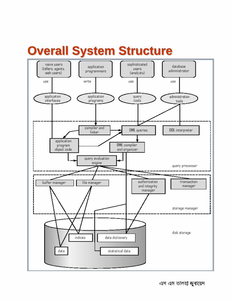
Overall System Structure

A Modern Data Architecture
Purpose of Database Systems In the early days, database applications were built directly on top of file systems
Drawbacks of using file systems to store data:
Data redundancy and inconsistency Multiple file formats, duplication of information in different files
Difficulty in accessing data Need to write a new program to carry out each new task
Data isolation — multiple files and formats
Integrity problems Integrity constraints (e.g. account balance > 0) become “buried” in
program code rather than being stated explicitly Hard to add new constraints or change existing ones
Atomicity of updates Failures may leave database in an inconsistent state with partial updates
carried out Example: Transfer of funds from one account to another should either
complete or not happen at all
Concurrent access by multiple users Concurrent accessed needed for performance Uncontrolled concurrent accesses can lead to inconsistencies
– Example: Two people reading a balance and updating it at the same time
Security problems Hard to provide user access to some, but not all, data
Database systems offer solutions to all the above problems
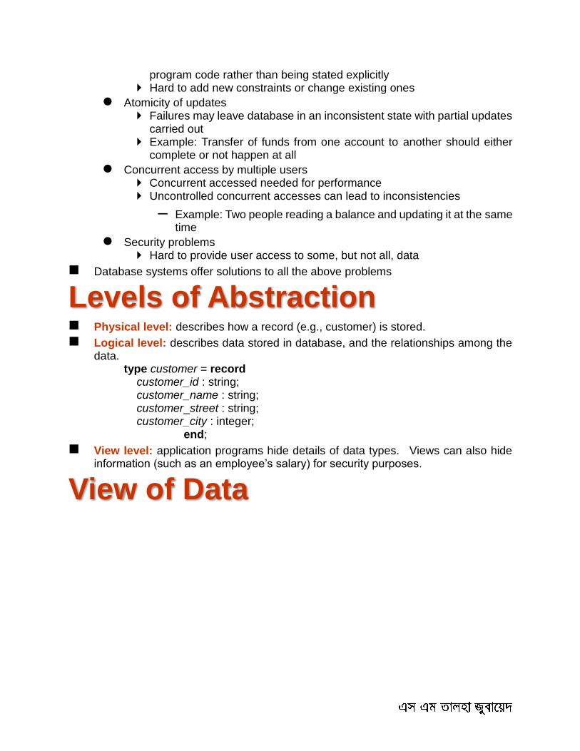
Levels of Abstraction Physical level: describes how a record (e.g., customer) is stored.
Logical level: describes data stored in database, and the relationships among the data.
type customer = record customer_id : string;
customer_name : string; customer_street : string; customer_city : integer;
end;
View level: application programs hide details of data types. Views can also hide information (such as an employee’s salary) for security purposes.
View of Data
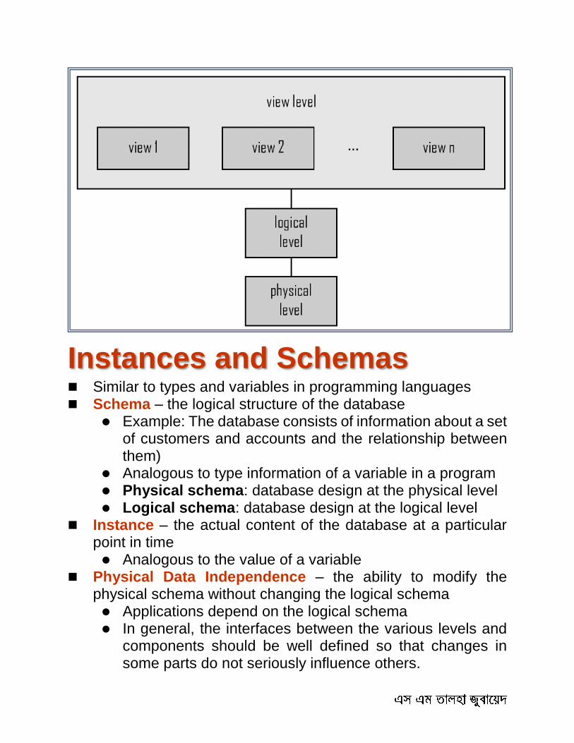
Instances and Schemas Similar to types and variables in programming languages Schema – the logical structure of the database
Example: The database consists of information about a set of customers and accounts and the relationship between them)
Analogous to type information of a variable in a program Physical schema: database design at the physical level Logical schema: database design at the logical level
Instance – the actual content of the database at a particular point in time Analogous to the value of a variable
Physical Data Independence – the ability to modify the physical schema without changing the logical schema Applications depend on the logical schema In general, the interfaces between the various levels and
components should be well defined so that changes in some parts do not seriously influence others.
Data Models A collection of tools for describing
Data
Data relationships
Data semantics
Data constraints
Relational model
Entity-Relationship data model (mainly for database design)
Object-based data models (Object-oriented and Object-relational)
Semistructured data model (XML)
Other older models:
Network model
Hierarchical model
Data Manipulation Language
(DML) Language for accessing and manipulating the data organized by the appropriate
data model
DML also known as query language
Retrieval of information
Insertion of new information
Deletion of information
Modification of information
Two classes of languages
Procedural – user specifies what data is required and how to get those data
Declarative (nonprocedural) – user specifies what data is required without specifying how to get those data
SQL is the most widely used query language
Data Definition Language
(DDL) Specification notation for defining the database schema

Example: create table account ( account-number char(10), balance integer)
DDL compiler generates a set of tables stored in a data dictionary
Data dictionary contains metadata (i.e., data about data)
Database schema
Data storage and definition language Specifies the storage structure and access methods used
Integrity constraints Domain constraints Referential integrity (references constraint in SQL) Assertions Authorization
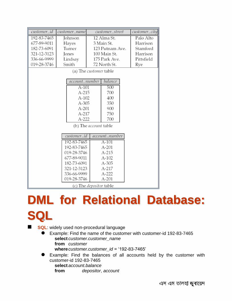
Relational Model Example of tabular data in the relational model
A Sample Relational Database
Attributes
DML for Relational Database:
SQL SQL: widely used non-procedural language
Example: Find the name of the customer with customer-id 192-83-7465 select customer.customer_name from customer where customer.customer_id = ‘192-83-7465’
Example: Find the balances of all accounts held by the customer with customer-id 192-83-7465 select account.balance from depositor, account
where depositor.customer_id = ‘192-83-7465’ and depositor.account_number = account.account_number
Application programs generally access databases through one of
Language extensions to allow embedded SQL
Application program interface (e.g., ODBC/JDBC) which allow SQL queries to be sent to a database
Database Design The process of designing the general structure of the database:
Logical Design – Deciding on the database schema. Database design requires that we find a “good” collection of relation schemas.
Business decision – What attributes should we record in the database?
Computer Science decision – What relation schemas should we have and how should the attributes be distributed among the various relation schemas?
Physical Design – Deciding on the physical layout of the database
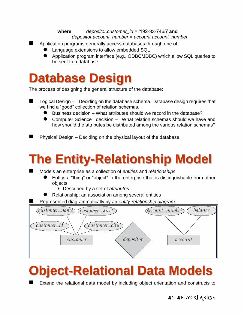
The Entity-Relationship Model Models an enterprise as a collection of entities and relationships
Entity: a “thing” or “object” in the enterprise that is distinguishable from other objects Described by a set of attributes
Relationship: an association among several entities
Represented diagrammatically by an entity-relationship diagram:
Object-Relational Data Models Extend the relational data model by including object orientation and constructs to

deal with added data types.
Allow attributes of tuples to have complex types, including non-atomic values such as nested relations.
Preserve relational foundations, in particular the declarative access to data, while extending modeling power.
Provide upward compatibility with existing relational languages.
XML: Extensible Markup
Language Defined by the WWW Consortium (W3C)
Originally intended as a document markup language not a database language
The ability to specify new tags, and to create nested tag structures made XML a great way to exchange data, not just documents
XML has become the basis for all new generation data interchange formats.
A wide variety of tools is available for parsing, browsing and querying XML documents/data
Storage Management Storage manager is a program module that provides the interface between the low-
level data stored in the database and the application programs and queries submitted to the system.
The storage manager is responsible to the following tasks:
Interaction with the file manager
Efficient storing, retrieving and updating of data
Components:
Authorization and integrity manager
Transaction manager
File manager
Buffer manager
Issues:
Storage access
File organization
Indexing and hashing
Query Processing 1. Parsing and translation 2. Optimization

3. Evaluation
Alternative ways of evaluating a given query
Equivalent expressions
Different algorithms for each operation
Cost difference between a good and a bad way of evaluating a query can be enormous
Need to estimate the cost of operations
Depends critically on statistical information about relations which the database must maintain
Need to estimate statistics for intermediate results to compute cost of complex expressions
Transaction Management A transaction is a collection of operations that performs a single logical function in
a database application
Transaction-management component ensures that the database remains in a consistent (correct) state despite system failures (e.g., power failures and operating system crashes) and transaction failures.
Concurrency-control manager controls the interaction among the concurrent transactions, to ensure the consistency of the database.

Database Architecture The architecture of a database systems is greatly influenced by the underlying computer system on which the database is running:
Centralized
Client-server
Parallel (multi-processor)
Distributed
Database Users Users are differentiated by the way they expect to interact with the system
Application programmers – interact with system through DML calls
Sophisticated users – form requests in a database query language
Specialized users – write specialized database applications that do not fit into the traditional data processing framework
Naïve users – invoke one of the permanent application programs that have been written previously
Examples, people accessing database over the web, bank tellers, clerical staff
Database Administrator Coordinates all the activities of the database system; the database administrator has
a good understanding of the enterprise’s information resources and needs.
Database administrator's duties include:
Schema definition
Storage structure and access method definition
Schema and physical organization modification
Granting user authority to access the database
Specifying integrity constraints
Acting as liaison with users
Monitoring performance and responding to changes in requirements

History of Database Systems 1950s and early 1960s:
Data processing using magnetic tapes for storage Tapes provide only sequential access
Punched cards for input
Late 1960s and 1970s:
Hard disks allow direct access to data
Network and hierarchical data models in widespread use
Ted Codd defines the relational data model Would win the ACM Turing Award for this work IBM Research begins System R prototype UC Berkeley begins Ingres prototype
High-performance (for the era) transaction processing
1980s:
Research relational prototypes evolve into commercial systems SQL becomes industrial standard
Parallel and distributed database systems
Object-oriented database systems
1990s:
Large decision support and data-mining applications
Large multi-terabyte data warehouses
Emergence of Web commerce

2000s:
XML and XQuery standards
Automated database administration

2014
11/16/2014
Relational Model Structure of Relational Databases
Fundamental Relational-Algebra-Operations
Additional Relational-Algebra-Operations
Extended Relational-Algebra-Operations
Null Values
Modification of the Database
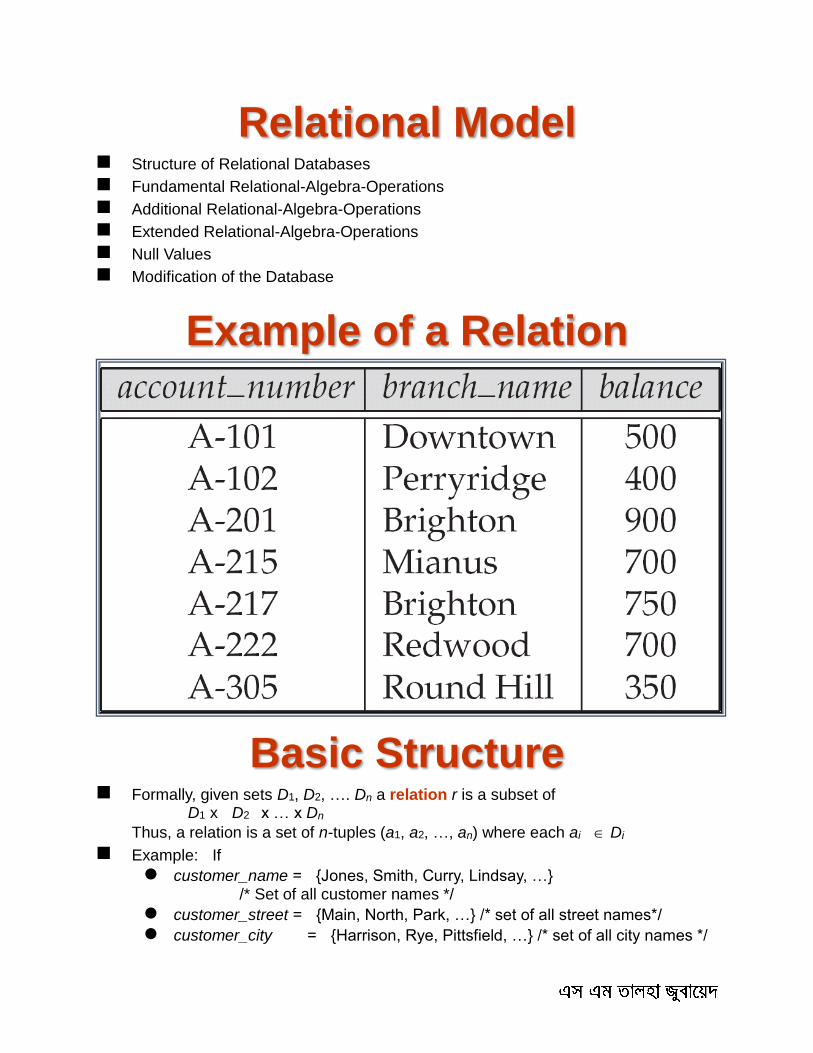
Example of a Relation
Basic Structure Formally, given sets D1, D2, …. Dn a relation r is a subset of
D1 x D2 x … x Dn
Thus, a relation is a set of n-tuples (a1, a2, …, an) where each ai Di
Example: If
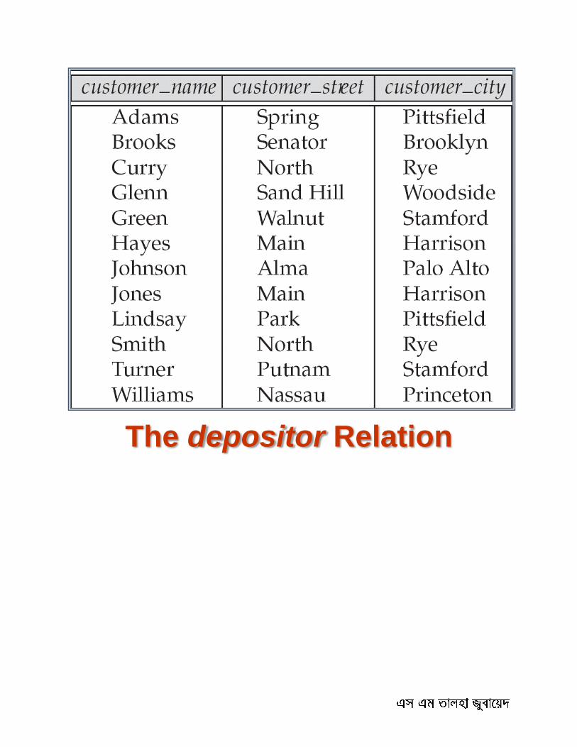
customer_name = {Jones, Smith, Curry, Lindsay, …} /* Set of all customer names */
customer_street = {Main, North, Park, …} /* set of all street names*/
customer_city = {Harrison, Rye, Pittsfield, …} /* set of all city names */
Then r = { (Jones, Main, Harrison), (Smith, North, Rye), (Curry, North, Rye), (Lindsay, Park, Pittsfield) } is a relation over
customer_name x customer_street x customer_city
Attribute Types Each attribute of a relation has a name
The set of allowed values for each attribute is called the domain of the attribute
Attribute values are (normally) required to be atomic; that is, indivisible
E.g. the value of an attribute can be an account number, but cannot be a set of account numbers
Domain is said to be atomic if all its members are atomic
The special value null is a member of every domain
The null value causes complications in the definition of many operations
We shall ignore the effect of null values in our main presentation and consider their effect later
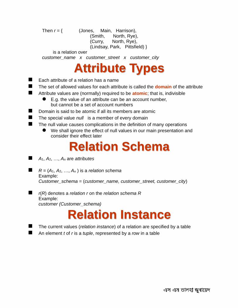
Relation Schema A1, A2, …, An are attributes
R = (A1, A2, …, An ) is a relation schema Example: Customer_schema = (customer_name, customer_street, customer_city)
r(R) denotes a relation r on the relation schema R Example: customer (Customer_schema)
Relation Instance The current values (relation instance) of a relation are specified by a table
An element t of r is a tuple, represented by a row in a table
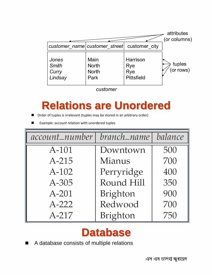
Relations are Unordered Order of tuples is irrelevant (tuples may be stored in an arbitrary order)
Example: account relation with unordered tuples
Database A database consists of multiple relations
Information about an enterprise is broken up into parts, with each relation storing one part of the information
account : stores information about accounts depositor : stores information about which customer owns which account customer : stores information about customers
Storing all information as a single relation such as bank(account_number, balance, customer_name, ..) results in repetition of information
e.g.,if two customers own an account (What gets repeated?)
the need for null values e.g., to represent a customer without an account
Normalization theory deals with how to design relational schemas
The customer Relation
The depositor Relation
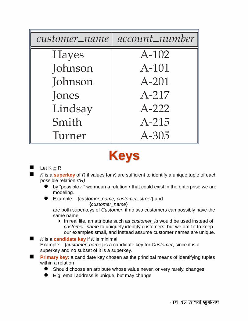
Keys Let K R
K is a superkey of R if values for K are sufficient to identify a unique tuple of each possible relation r(R)
by “possible r ” we mean a relation r that could exist in the enterprise we are modeling.
Example: {customer_name, customer_street} and {customer_name} are both superkeys of Customer, if no two customers can possibly have the same name In real life, an attribute such as customer_id would be used instead of
customer_name to uniquely identify customers, but we omit it to keep our examples small, and instead assume customer names are unique.
K is a candidate key if K is minimal Example: {customer_name} is a candidate key for Customer, since it is a superkey and no subset of it is a superkey.
Primary key: a candidate key chosen as the principal means of identifying tuples within a relation
Should choose an attribute whose value never, or very rarely, changes.
E.g. email address is unique, but may change
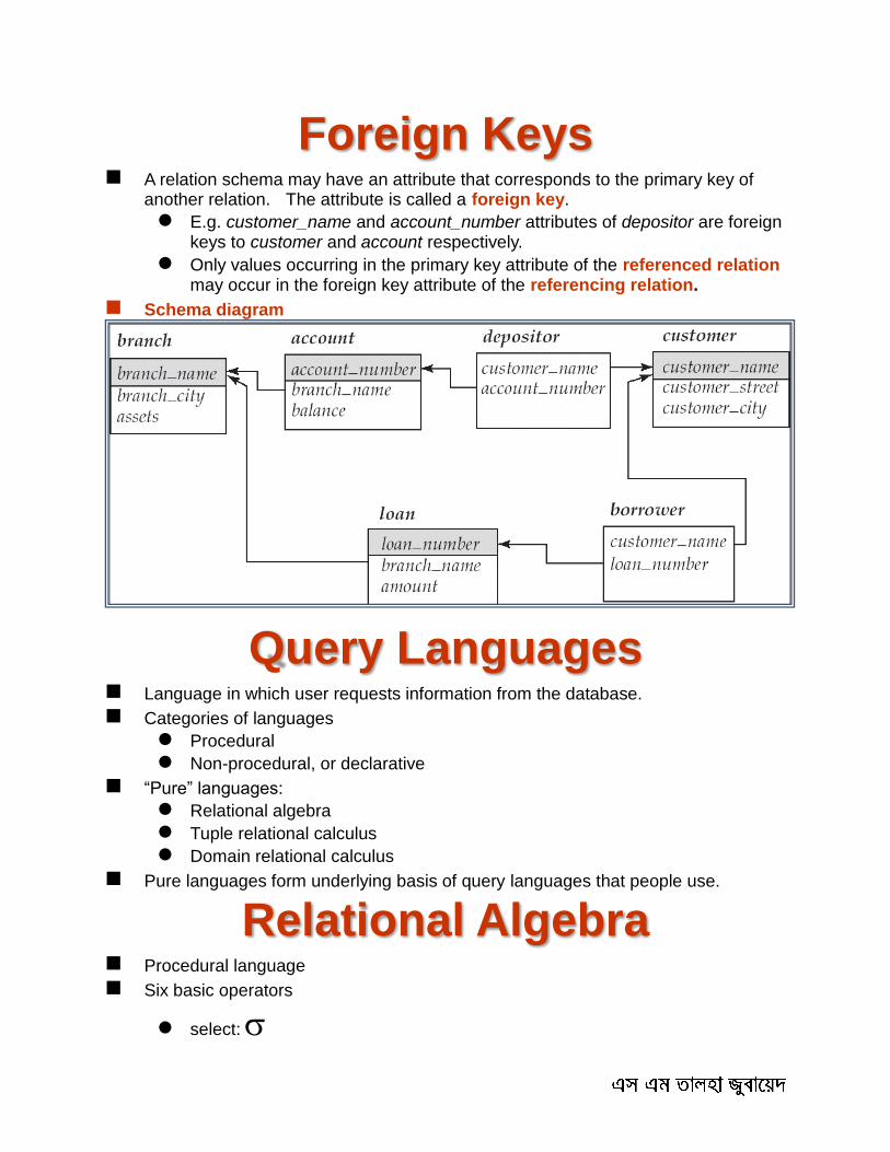
Foreign Keys A relation schema may have an attribute that corresponds to the primary key of
another relation. The attribute is called a foreign key.
E.g. customer_name and account_number attributes of depositor are foreign keys to customer and account respectively.
Only values occurring in the primary key attribute of the referenced relation may occur in the foreign key attribute of the referencing relation.
Schema diagram
Query Languages Language in which user requests information from the database.
Categories of languages
Procedural
Non-procedural, or declarative
“Pure” languages:
Relational algebra
Tuple relational calculus
Domain relational calculus
Pure languages form underlying basis of query languages that people use.
Relational Algebra Procedural language
Six basic operators
select:
project:
union:
set difference: –
Cartesian product: x
rename:
The operators take one or two relations as inputs and produce a new relation as a result.
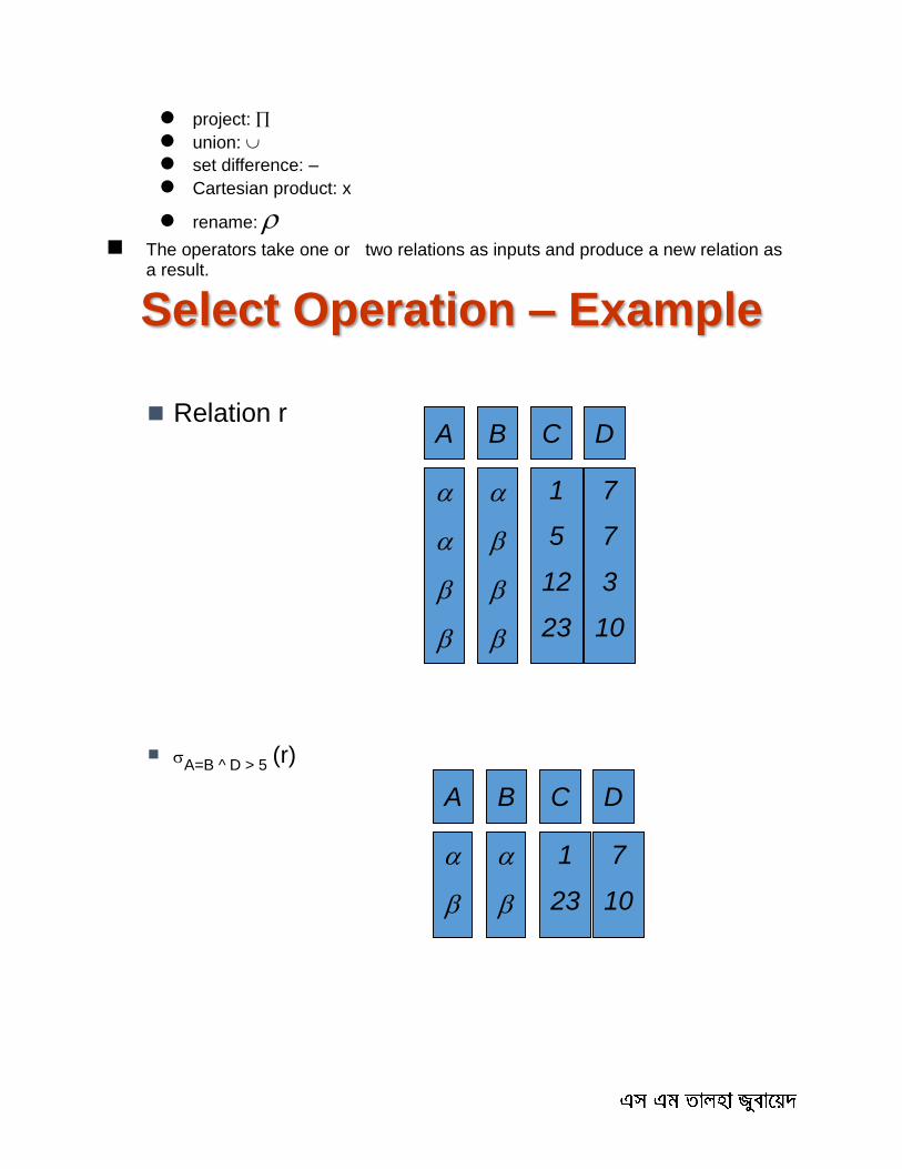
Select Operation – Example
Relation r A B C D
1
5
12
23
7
7
3
10
A=B ^ D > 5
(r)
A B C D
1
23
7
10

Select Operation Notation: p(r) p is called the selection predicate Defined as:
p(r) = {t | t r and p(t)}
Where p is a formula in propositional calculus consisting of terms and or not) Each term is one of:
<attribute> op <attribute> or <constant> where op
Example of selection:
branch_name=“Perryridge”(account)
Project Operation – Example
Project Operation Notation:
where A1, A2 are attribute names and r is a relation name.
The result is defined as the relation of k columns obtained by erasing the columns that are not listed
Duplicate rows removed from result, since relations are sets
Example: To eliminate the branch_name attribute of account
account_number, balance (account)
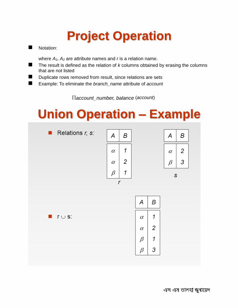
Union Operation – Example
Union Operation Notation: r s
Defined as:
r s = {t | t r or t s}
For r s to be valid. 1. r, s must have the same arity (same number of attributes) 2. The attribute domains must be compatible (example: 2nd column
of r deals with the same type of values as does the 2nd column of s)
Example: to find all customers with either an account or a loan
customer_name (depositor) customer_name (borrower)
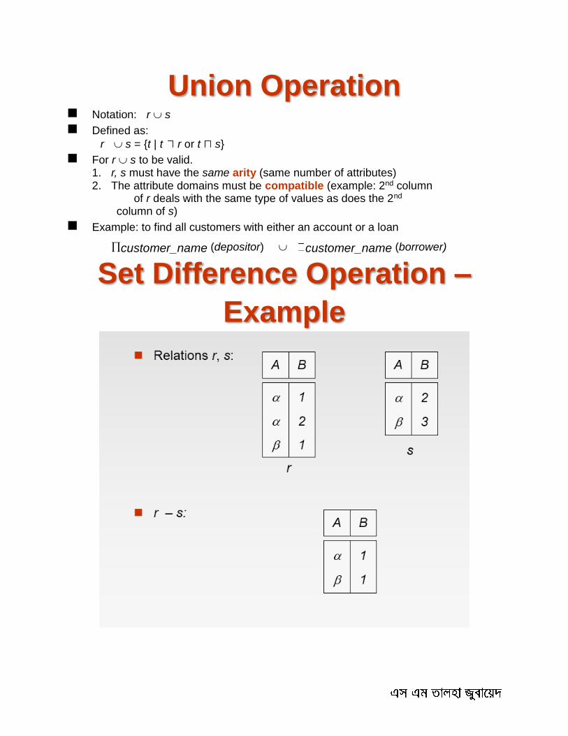
Set Difference Operation –
Example
Set Difference Operation Notation r – s
Defined as:
r – s = {t | t r and s}
Set differences must be taken between compatible relations.
r and s must have the same arity
attribute domains of r and s must be compatible
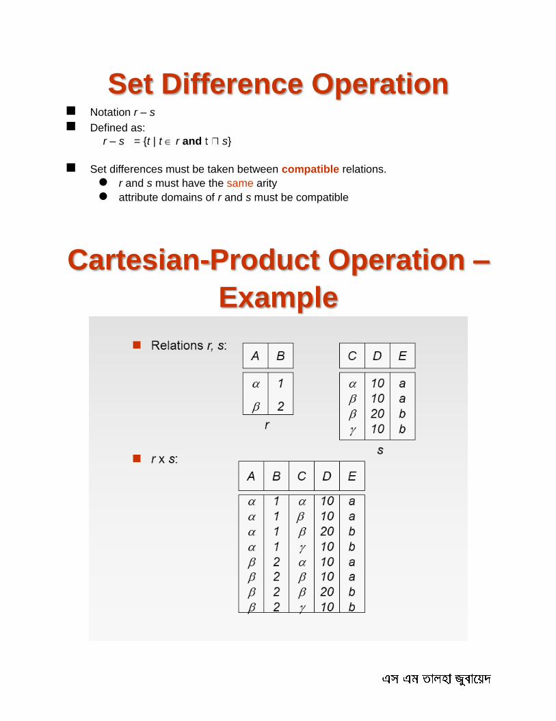
Cartesian-Product Operation –
Example
Cartesian-Product Operation Notation r x s
Defined as:
r x s = {t q | t r and q s}
Assume that attributes of r(R) and s(S) are disjoint. (That is, R S = ).
If attributes of r(R) and s(S) are not disjoint, then renaming must be used.
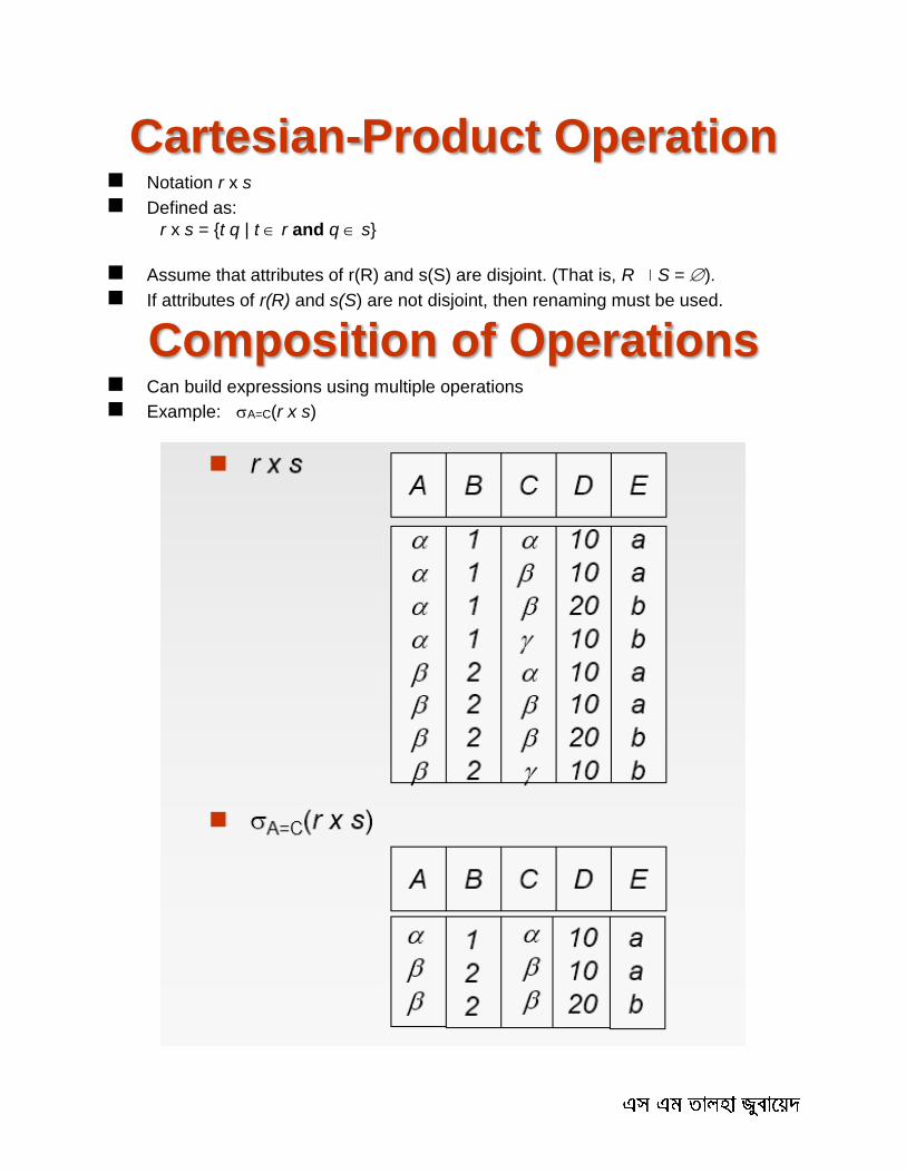
Composition of Operations Can build expressions using multiple operations
Example: A=C(r x s)

A=C(r x s)
Rename Operation Allows us to name, and therefore to refer to, the results of relational-algebra
expressions.
Allows us to refer to a relation by more than one name.
Example:
x (E)
returns the expression E under the name X
If a relational-algebra expression E has arity n, then returns the result of expression E under the name X, and with the
attributes renamed to A1 , A2 , …., An .
Banking Example branch (branch_name, branch_city, assets)
customer (customer_name, customer_street, customer_city) account (account_number, branch_name, balance) loan (loan_number, branch_name, amount) depositor (customer_name, account_number) borrower (customer_name, loan_number)
Example Queries Find all loans of over $1200
amount > 1200
(loan)

Find the loan number for each loan of an amount greater than $1200
Find the names of all customers who have a loan, an account, or both, from the bank
loan_number
(amount
> 1200
(loan))
customer_name
(borrower) customer_name
(depositor)

Find the largest account balance Strategy:
Find those balances that are not the largest
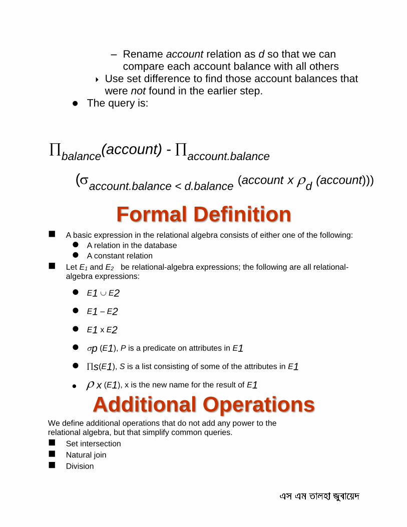
– Rename account relation as d so that we can compare each account balance with all others
Use set difference to find those account balances that were not found in the earlier step.
The query is:
Formal Definition A basic expression in the relational algebra consists of either one of the following:
A relation in the database
A constant relation
Let E1 and E2 be relational-algebra expressions; the following are all relational-algebra expressions:
E1 E2 E1 – E2 E1 x E2 p (E1), P is a predicate on attributes in E1 s(E1), S is a list consisting of some of the attributes in E1
x (E1), x is the new name for the result of E1
Additional Operations We define additional operations that do not add any power to the relational algebra, but that simplify common queries.
Set intersection
Natural join
Division
balance
(account) - account.balance
(account.balance < d.balance
(account x d (account)))
Assignment
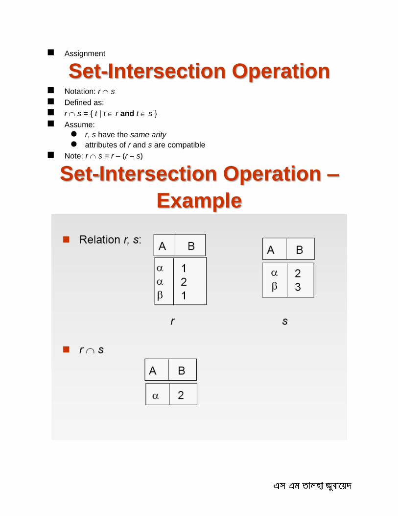
Set-Intersection Operation Notation: r s
Defined as:
r s = { t | t r and t s }
Assume:
r, s have the same arity
attributes of r and s are compatible
Note: r s = r – (r – s)
Set-Intersection Operation –
Example

Natural-Join Operation Let r and s be relations on schemas R and S respectively.
Then, r s is a relation on schema R S obtained as follows:
Consider each pair of tuples tr from r and ts from s.
If tr and ts have the same value on each of the attributes in R S, add a
tuple t to the result, where
t has the same value as tr on r
t has the same value as ts on s
Example: R = (A, B, C, D) S = (E, B, D)
Result schema = (A, B, C, D, E)
r s is defined as:
r.A, r.B, r.C, r.D, s.E (r.B = s.B r.D = s.D (r x s))
Natural Join Operation –
Example
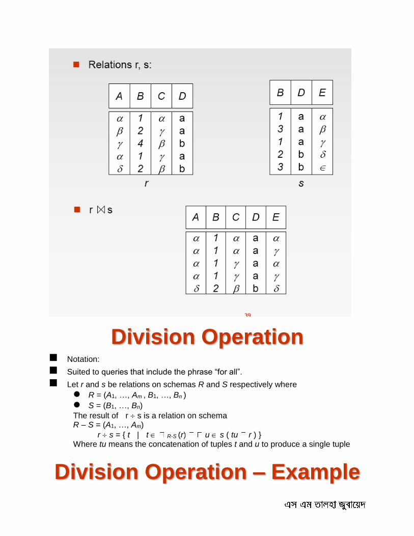
Division Operation Notation:
Suited to queries that include the phrase “for all”.
Let r and s be relations on schemas R and S respectively where
R = (A1, …, Am , B1, …, Bn )
S = (B1, …, Bn)
The result of r s is a relation on schema R – S = (A1, …, Am)
r s = { t | t R-S (r u s ( tu r ) } Where tu means the concatenation of tuples t and u to produce a single tuple
Division Operation – Example
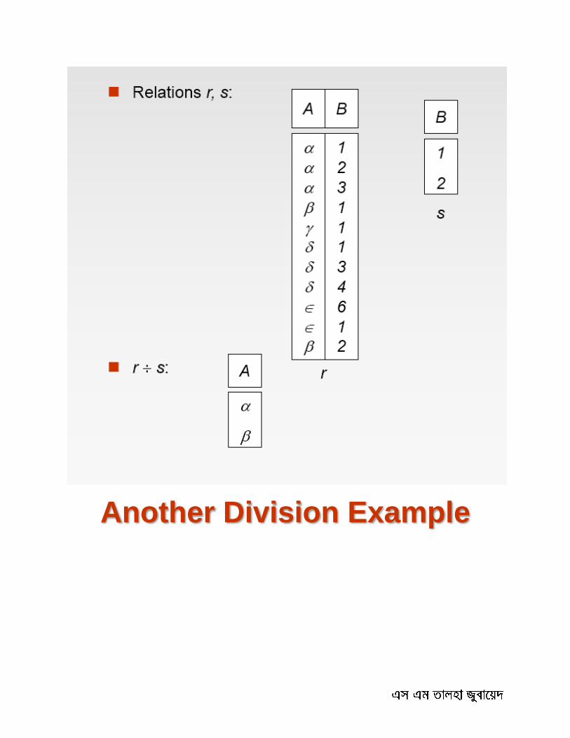
Another Division Example
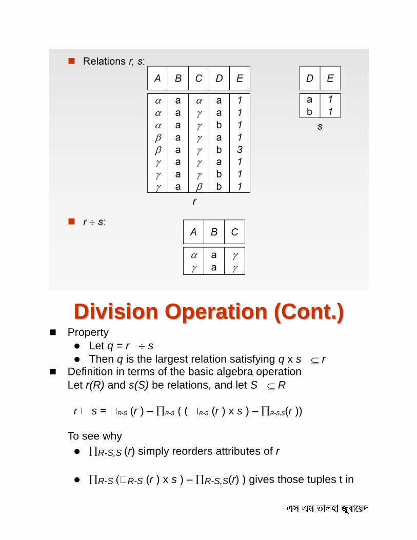
Division Operation (Cont.) Property
Let q = r s
Then q is the largest relation satisfying q x s r Definition in terms of the basic algebra operation
Let r(R) and s(S) be relations, and let S R
r s R-S (r ) – R-S R-S (r ) x s ) – R-S,S(r ))
To see why
R-S,S (r) simply reorders attributes of r
R-S R-S (r ) x s ) – R-S,S(r) ) gives those tuples t in
R-S (r ) such that for some tuple u s, tu r.
Assignment Operation The assignment operation () provides a convenient way to
express complex queries. Write query as a sequential program consisting of
a series of assignments followed by an expression whose value is displayed
as a result of the query. Assignment must always be made to a temporary relation
variable. Example: Write r s as
temp1 R-S (r )
temp2 R-S ((temp1 x s ) – R-S,S (r )) result = temp1 – temp2
May use variable in subsequent expressions.
Bank Example Queries
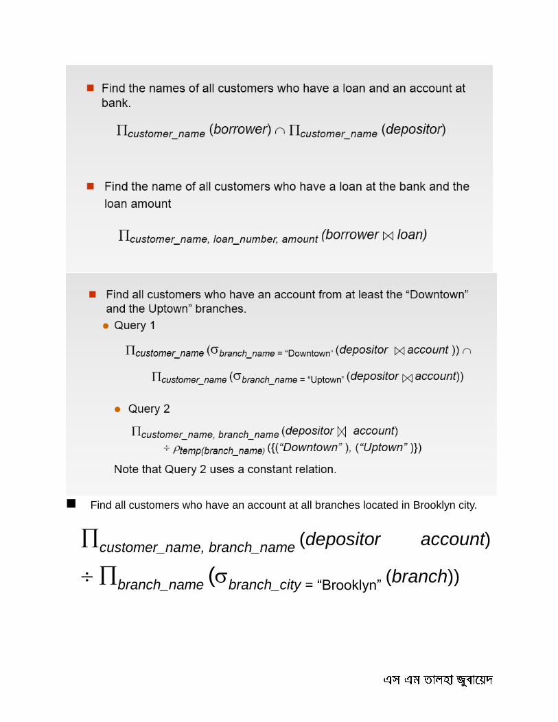
Find all customers who have an account at all branches located in Brooklyn city.
customer_name, branch_name
(depositor account)
branch_name
(branch_city = “Brooklyn”
(branch))
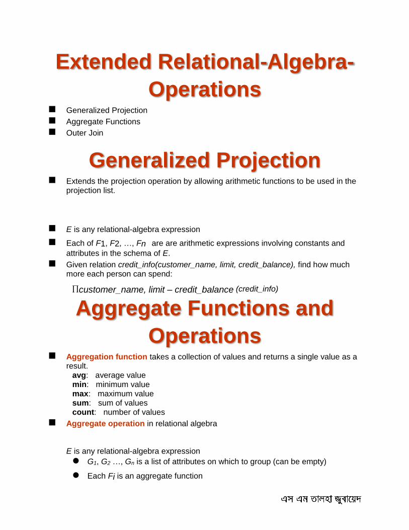
Extended Relational-Algebra-
Operations Generalized Projection
Aggregate Functions
Outer Join
Generalized Projection Extends the projection operation by allowing arithmetic functions to be used in the
projection list.
E is any relational-algebra expression
Each of F1, F2, …, Fn are are arithmetic expressions involving constants and
attributes in the schema of E.
Given relation credit_info(customer_name, limit, credit_balance), find how much more each person can spend:
customer_name, limit – credit_balance (credit_info)
Aggregate Functions and
Operations Aggregation function takes a collection of values and returns a single value as a
result. avg: average value
min: minimum value max: maximum value sum: sum of values count: number of values
Aggregate operation in relational algebra
E is any relational-algebra expression
G1, G2 …, Gn is a list of attributes on which to group (can be empty)
Each Fi is an aggregate function

Each Ai is an attribute name
Aggregate Operation –
Example
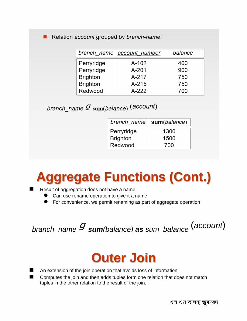
Aggregate Functions (Cont.) Result of aggregation does not have a name
Can use rename operation to give it a name
For convenience, we permit renaming as part of aggregate operation
Outer Join An extension of the join operation that avoids loss of information.
Computes the join and then adds tuples form one relation that does not match tuples in the other relation to the result of the join.
branch_name g
sum(balance) as sum_balance (account)
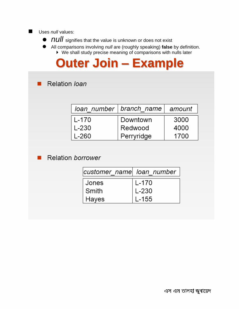
Uses null values:
null signifies that the value is unknown or does not exist
All comparisons involving null are (roughly speaking) false by definition. We shall study precise meaning of comparisons with nulls later
Outer Join – Example

Null Values It is possible for tuples to have a null value, denoted by null, for some of their
attributes
null signifies an unknown value or that a value does not exist.
The result of any arithmetic expression involving null is null.
Aggregate functions simply ignore null values (as in SQL)
For duplicate elimination and grouping, null is treated like any other value, and two nulls are assumed to be the same (as in SQL)
Comparisons with null values return the special truth value: unknown
If false was used instead of unknown, then not (A < 5) would not be equivalent to A >= 5
Three-valued logic using the truth value unknown:
OR: (unknown or true) = true, (unknown or false) = unknown (unknown or unknown) = unknown
AND: (true and unknown) = unknown, (false and unknown) = false, (unknown and unknown) = unknown
NOT: (not unknown) = unknown
In SQL “P is unknown” evaluates to true if predicate P evaluates to unknown
Result of select predicate is treated as false if it evaluates to unknown
Modification of the Database The content of the database may be modified using the following operations:
Deletion
Insertion
Updating
All these operations are expressed using the assignment operator.
Deletion A delete request is expressed similarly to a query, except instead of displaying
tuples to the user, the selected tuples are removed from the database.
Can delete only whole tuples; cannot delete values on only particular attributes
A deletion is expressed in relational algebra by:
r r – E where r is a relation and E is a relational algebra query.
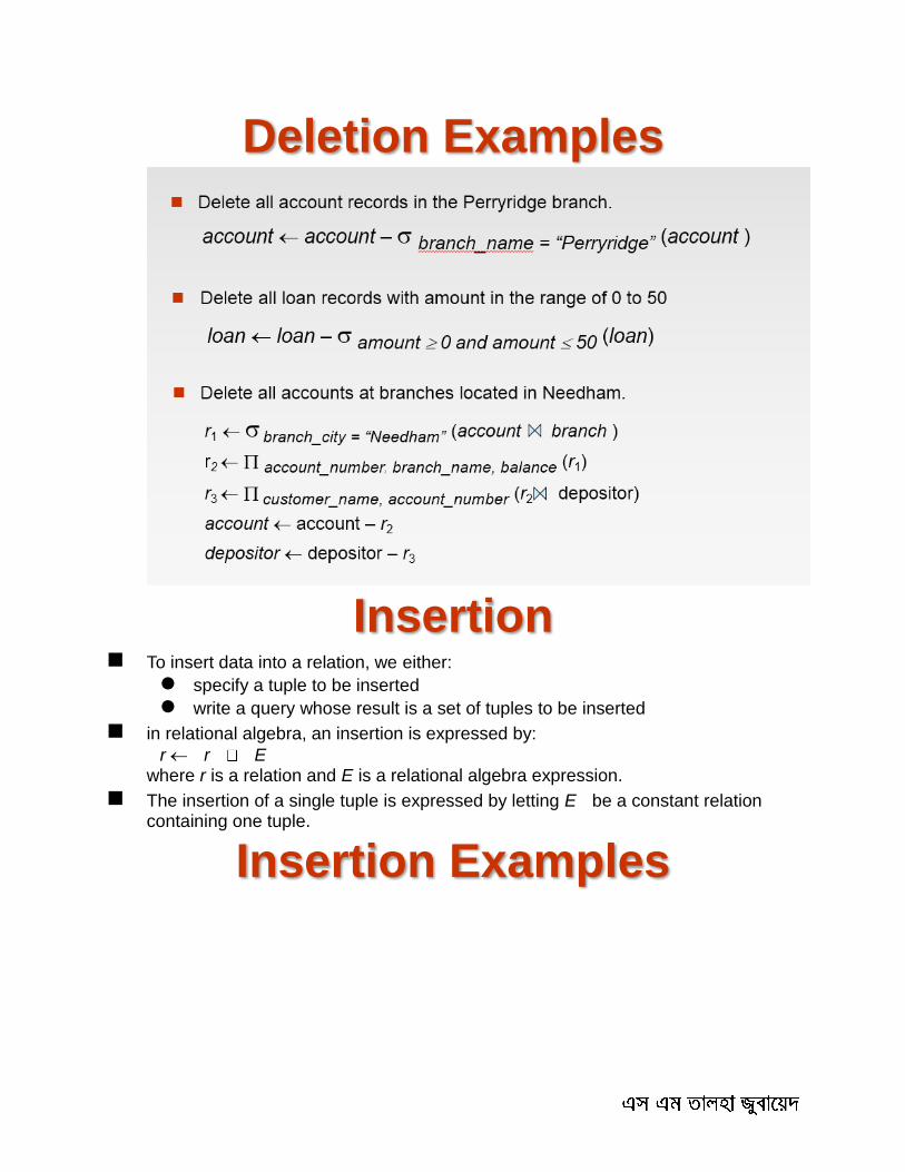
Deletion Examples
Insertion To insert data into a relation, we either:
specify a tuple to be inserted
write a query whose result is a set of tuples to be inserted
in relational algebra, an insertion is expressed by:
r r E where r is a relation and E is a relational algebra expression.
The insertion of a single tuple is expressed by letting E be a constant relation containing one tuple.
Insertion Examples
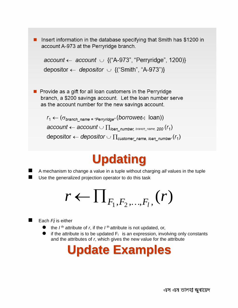
Updating A mechanism to change a value in a tuple without charging all values in the tuple
Use the generalized projection operator to do this task
)(,,,, 21rr
lFFF
Each Fi is either
the I th attribute of r, if the I th attribute is not updated, or,
if the attribute is to be updated Fi is an expression, involving only constants and the attributes of r, which gives the new value for the attribute
Update Examples

2014
11/16/2014
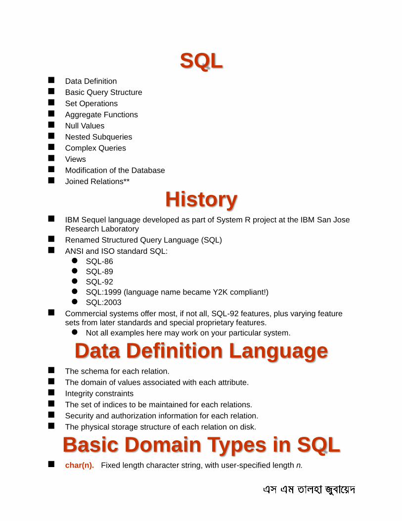
SQL Data Definition
Basic Query Structure
Set Operations
Aggregate Functions
Null Values
Nested Subqueries
Complex Queries
Views
Modification of the Database
Joined Relations**
History IBM Sequel language developed as part of System R project at the IBM San Jose
Research Laboratory
Renamed Structured Query Language (SQL)
ANSI and ISO standard SQL:
SQL-86
SQL-89
SQL-92
SQL:1999 (language name became Y2K compliant!)
SQL:2003
Commercial systems offer most, if not all, SQL-92 features, plus varying feature sets from later standards and special proprietary features.
Not all examples here may work on your particular system.
Data Definition Language The schema for each relation.
The domain of values associated with each attribute.
Integrity constraints
The set of indices to be maintained for each relations.
Security and authorization information for each relation.
The physical storage structure of each relation on disk.
Basic Domain Types in SQL char(n). Fixed length character string, with user-specified length n.
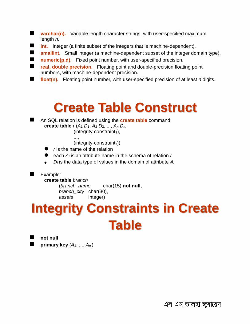
varchar(n). Variable length character strings, with user-specified maximum length n.
int. Integer (a finite subset of the integers that is machine-dependent).
smallint. Small integer (a machine-dependent subset of the integer domain type).
numeric(p,d). Fixed point number, with user-specified precision.
real, double precision. Floating point and double-precision floating point numbers, with machine-dependent precision.
float(n). Floating point number, with user-specified precision of at least n digits.
Create Table Construct An SQL relation is defined using the create table command: create table r (A1 D1, A2 D2, ..., An Dn,
(integrity-constraint1), ..., (integrity-constraintk))
r is the name of the relation
each Ai is an attribute name in the schema of relation r
Di is the data type of values in the domain of attribute Ai
Example: create table branch
(branch_name char(15) not null, branch_city char(30), assets integer)
Integrity Constraints in Create
Table not null
primary key (A1, ..., An )
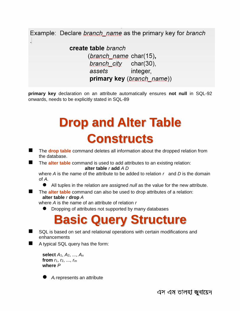
primary key declaration on an attribute automatically ensures not null in SQL-92
onwards, needs to be explicitly stated in SQL-89
Drop and Alter Table
Constructs The drop table command deletes all information about the dropped relation from
the database.
The alter table command is used to add attributes to an existing relation: alter table r add A D where A is the name of the attribute to be added to relation r and D is the domain
of A.
All tuples in the relation are assigned null as the value for the new attribute.
The alter table command can also be used to drop attributes of a relation: alter table r drop A where A is the name of an attribute of relation r
Dropping of attributes not supported by many databases
Basic Query Structure SQL is based on set and relational operations with certain modifications and
enhancements
A typical SQL query has the form: select A1, A2, ..., An from r1, r2, ..., rm where P
Ai represents an attribute
ri represents a relation
P is a predicate.
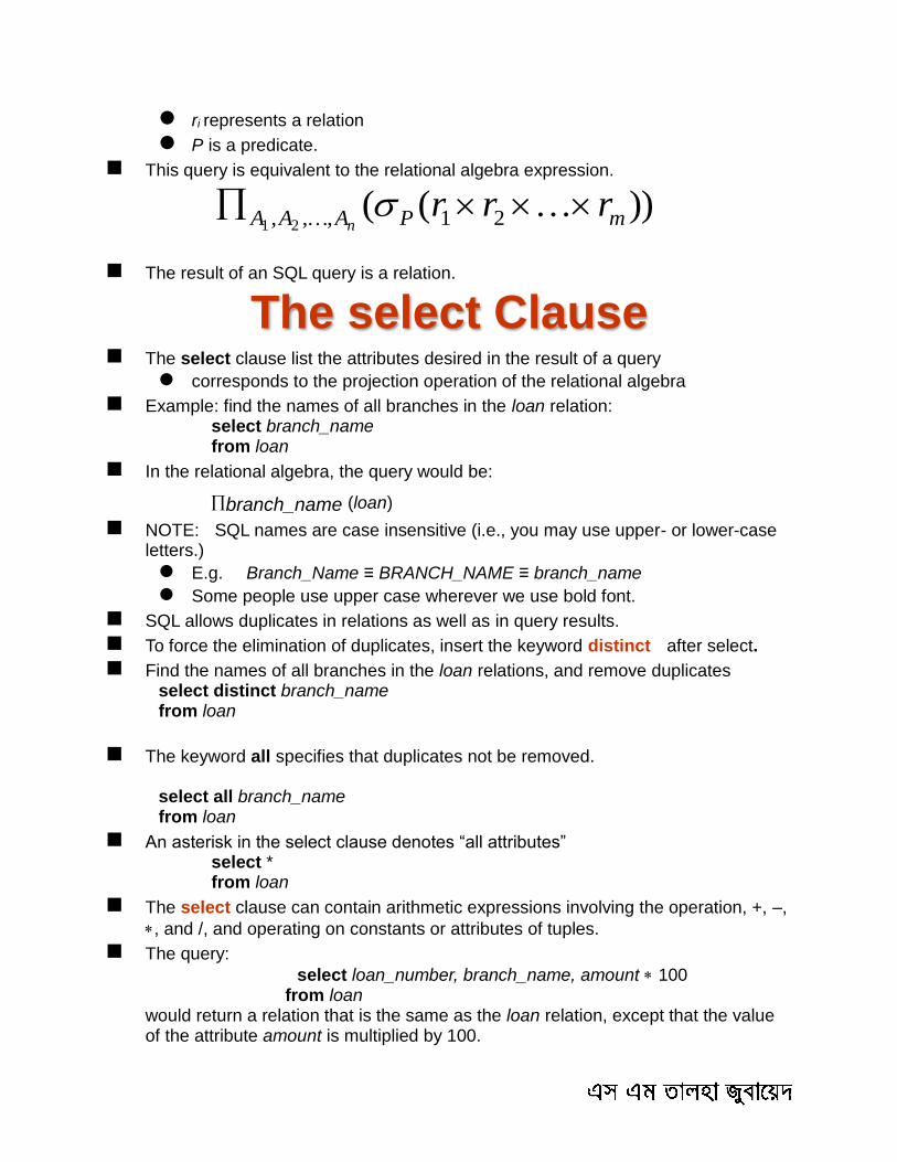
This query is equivalent to the relational algebra expression.
))(( 21,,, 21 mPAAA rrrn
The result of an SQL query is a relation.
The select Clause The select clause list the attributes desired in the result of a query
corresponds to the projection operation of the relational algebra
Example: find the names of all branches in the loan relation: select branch_name from loan
In the relational algebra, the query would be:
branch_name (loan)
NOTE: SQL names are case insensitive (i.e., you may use upper- or lower-case letters.)
E.g. Branch_Name ≡ BRANCH_NAME ≡ branch_name
Some people use upper case wherever we use bold font.
SQL allows duplicates in relations as well as in query results.
To force the elimination of duplicates, insert the keyword distinct after select.
Find the names of all branches in the loan relations, and remove duplicates select distinct branch_name
from loan
The keyword all specifies that duplicates not be removed.
select all branch_name from loan
An asterisk in the select clause denotes “all attributes” select *
from loan
The select clause can contain arithmetic expressions involving the operation, +, –,
, and /, and operating on constants or attributes of tuples.
The query:
select loan_number, branch_name, amount 100 from loan
would return a relation that is the same as the loan relation, except that the value of the attribute amount is multiplied by 100.

The where Clause The where clause specifies conditions that the result must satisfy
Corresponds to the selection predicate of the relational algebra.
To find all loan number for loans made at the Perryridge branch with loan amounts greater than $1200.
select loan_number from loan where branch_name = 'Perryridge' and amount > 1200
Comparison results can be combined using the logical connectives and, or, and not.
Comparisons can be applied to results of arithmetic expressions.
SQL includes a between comparison operator
Example: Find the loan number of those loans with loan amounts between
$90,000 and $100,000 (that is, $90,000 and $100,000)
The from Clause The from clause lists the relations involved in the query
Corresponds to the Cartesian product operation of the relational algebra.
Find the Cartesian product borrower X loan
select from borrower, loan
Find the name, loan number and loan amount of all customers
having a loan at the Perryridge branch.
select customer_name, borrower.loan_number, amount from borrower, loan where borrower.loan_number = loan.loan_number and branch_name = 'Perryridge'
The Rename Operation
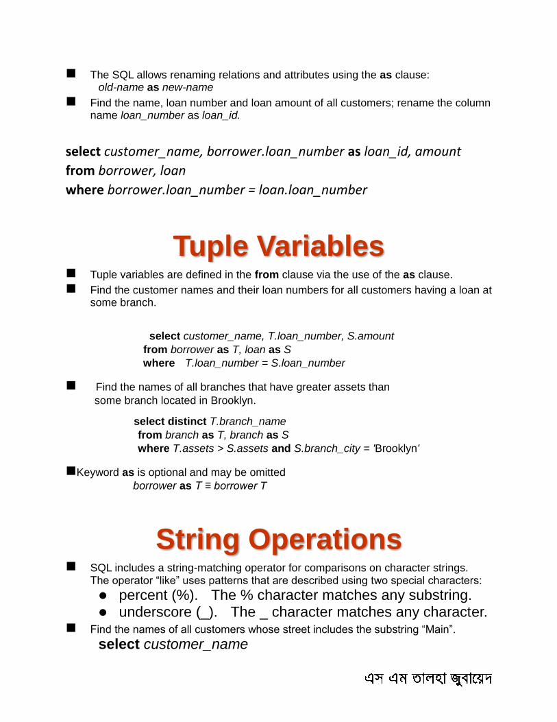
The SQL allows renaming relations and attributes using the as clause: old-name as new-name
Find the name, loan number and loan amount of all customers; rename the column name loan_number as loan_id.
select customer_name, borrower.loan_number as loan_id, amount
from borrower, loan
where borrower.loan_number = loan.loan_number
Tuple Variables Tuple variables are defined in the from clause via the use of the as clause.
Find the customer names and their loan numbers for all customers having a loan at some branch.
select customer_name, T.loan_number, S.amount
from borrower as T, loan as S
where T.loan_number = S.loan_number
Find the names of all branches that have greater assets than
some branch located in Brooklyn.
select distinct T.branch_name
from branch as T, branch as S
where T.assets > S.assets and S.branch_city = 'Brooklyn'
Keyword as is optional and may be omitted
borrower as T ≡ borrower T
String Operations SQL includes a string-matching operator for comparisons on character strings.
The operator “like” uses patterns that are described using two special characters:
percent (%). The % character matches any substring. underscore (_). The _ character matches any character.
Find the names of all customers whose street includes the substring “Main”.
select customer_name
from customer
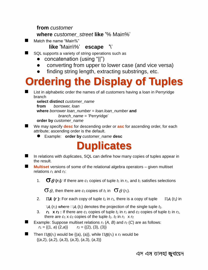
where customer_street like '% Main%' Match the name “Main%”
like 'Main\%' escape '\' SQL supports a variety of string operations such as
concatenation (using “||”) converting from upper to lower case (and vice versa) finding string length, extracting substrings, etc.
Ordering the Display of Tuples List in alphabetic order the names of all customers having a loan in Perryridge
branch select distinct customer_name
from borrower, loan where borrower loan_number = loan.loan_number and
branch_name = 'Perryridge' order by customer_name
We may specify desc for descending order or asc for ascending order, for each attribute; ascending order is the default.
Example: order by customer_name desc
Duplicates In relations with duplicates, SQL can define how many copies of tuples appear in
the result.
Multiset versions of some of the relational algebra operators – given multiset relations r1 and r2:
1. (r1): If there are c1 copies of tuple t1 in r1, and t1 satisfies selections
,, then there are c1 copies of t1 in (r1).
2. A (r ): For each copy of tuple t1 in r1, there is a copy of tuple A (t1) in
A (r1 A (t1) denotes the projection of the single tuple t1.
3. r1 x r2 : If there are c1 copies of tuple t1 in r1 and c2 copies of tuple t2 in r2, there are c1 x c2 copies of the tuple t1. t2 in r1 x r2
Example: Suppose multiset relations r1 (A, B) and r2 (C) are as follows: r1 = {(1, a) (2,a)} r2 = {(2), (3), (3)}
Then B(r1) would be {(a), (a)}, while B(r1) x r2 would be
{(a,2), (a,2), (a,3), (a,3), (a,3), (a,3)}
SQL duplicate semantics:
select A1,, A2, ..., An
from r1, r2, ..., rm
where P is equivalent to the multiset version of the expression:
))(( 21,,, 21 mPAAA rrrn
Set Operations The set operations union, intersect, and except operate on relations and
correspond to the relational algebra operations
Each of the above operations automatically eliminates duplicates; to retain all duplicates use the corresponding multiset versions union all, intersect all and except all. Suppose a tuple occurs m times in r and n times in s, then, it occurs:
m + n times in r union all s
min(m,n) times in r intersect all s
max(0, m – n) times in r except all s

Aggregate Functions These functions operate on the multiset of values of a column of a relation, and
return a value avg: average value
min: minimum value max: maximum value sum: sum of values count: number of values
Aggregate Functions – Group
By Find the number of depositors for each branch.
select branch_name, count (distinct customer_name)
from depositor, account
where depositor.account_number = account.account_number
group by branch_name
Note: Attributes in select clause outside of aggregate functions must
appear in group by list
Aggregate Functions – Having
Clause Find the names of all branches where the average account balance is more than
$1,200. select branch_name, avg (balance)
from account
group by branch_name
having avg (balance) > 1200
Note: predicates in the having clause are applied after the
formation of groups whereas predicates in the where
clause are applied before forming groups
Null Values It is possible for tuples to have a null value, denoted by null, for some of their
attributes
null signifies an unknown value or that a value does not exist.
The predicate is null can be used to check for null values.
Example: Find all loan number which appear in the loan relation with null values for amount.
select loan_number from loan where amount is null
The result of any arithmetic expression involving null is null
Example: 5 + null returns null
However, aggregate functions simply ignore nulls
More on next slide
Null Values and Three Valued
Logic Any comparison with null returns unknown
Example: 5 < null or null <> null or null = null
Three-valued logic using the truth value unknown:
OR: (unknown or true) = true, (unknown or false) = unknown (unknown or unknown) = unknown
AND: (true and unknown) = unknown, (false and unknown) = false, (unknown and unknown) = unknown
NOT: (not unknown) = unknown
“P is unknown” evaluates to true if predicate P evaluates to unknown
Result of where clause predicate is treated as false if it evaluates to unknown
Null Values and Aggregates Total all loan amounts select sum (amount )
from loan
Above statement ignores null amounts
Result is null if there is no non-null amount
All aggregate operations except count(*) ignore tuples with null values on the aggregated attributes.
Nested Subqueries SQL provides a mechanism for the nesting of subqueries.
A subquery is a select-from-where expression that is nested within another query.
A common use of subqueries is to perform tests for set membership, set comparisons, and set cardinality.
Example Query Find all customers who have both an account and a loan at the bank.
select distinct customer_name
from borrower
where customer_name in (select customer_name
from depositor )
Find all customers who have a loan at the bank but do not have
an account at the bank
select distinct customer_name
from borrower
where customer_name not in (select customer_name
from depositor )
Find all customers who have both an account and a loan at the Perryridge branch
select distinct customer_name
from borrower, loan
where borrower.loan_number = loan.loan_number and
branch_name = 'Perryridge' and
(branch_name, customer_name ) in
(select branch_name, customer_name
from depositor, account
where depositor.account_number =
account.account_number )
Note: Above query can be written in a much simpler manner. The
formulation above is simply to illustrate SQL features.
Set Comparison Find all branches that have greater assets than some branch located in Brooklyn.
select distinct T.branch_name
from branch as T, branch as S
where T.assets > S.assets and
S.branch_city = 'Brooklyn'
Same query using > some clause
select branch_name
from branch
where assets > some
(select assets
from branch
where branch_city = 'Brooklyn')
Definition of Some Clause

Example Query Find the names of all branches that have greater assets than all branches located
in Brooklyn.
select branch_name
from branch
where assets > all
(select assets
from branch
where branch_city = 'Brooklyn')
Definition of all Clause
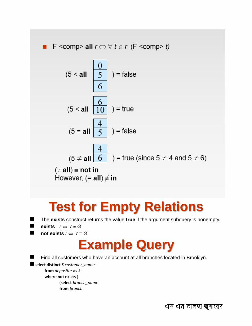
Test for Empty Relations The exists construct returns the value true if the argument subquery is nonempty.
exists r r Ø
not exists r r = Ø
Example Query Find all customers who have an account at all branches located in Brooklyn.
select distinct S.customer_name
from depositor as S
where not exists (
(select branch_name
from branch
where branch_city = 'Brooklyn')
except
(select R.branch_name
from depositor as T, account as R
where T.account_number = R.account_number and
S.customer_name = T.customer_name ))
Note that X – Y = Ø X Y
Note: Cannot write this query using = all and its variants
Test for Absence of Duplicate
Tuples The unique construct tests whether a subquery has any duplicate tuples in its
result.
Find all customers who have at most one account at the Perryridge branch. select T.customer_name from depositor as T where unique ( select R.customer_name
from account, depositor as R where T.customer_name = R.customer_name and R.account_number = account.account_number and account.branch_name = 'Perryridge')
Example Query Find all customers who have at least two accounts at the Perryridge branch. select distinct T.customer_name from depositor as T where not unique ( select R.customer_name from account, depositor as R where T.customer_name = R.customer_name and R.account_number = account.account_number and account.branch_name = 'Perryridge')
Variable from outer level is known as a correlation variable

Derived Relations SQL allows a subquery expression to be used in the from clause
Find the average account balance of those branches where the average account balance is greater than $1200.
select branch_name, avg_balance from (select branch_name, avg (balance) from account group by branch_name ) as branch_avg ( branch_name, avg_balance ) where avg_balance > 1200
Note that we do not need to use the having clause, since we compute the temporary (view) relation branch_avg in the from clause, and the attributes of branch_avg can be used directly in the where clause.
With Clause The with clause provides a way of defining a temporary view whose definition is
available only to the query in which the with clause occurs.
Find all accounts with the maximum balance with max_balance (value) as select max (balance) from account select account_number from account, max_balance where account.balance = max_balance.value
Complex Queries using With
Clause Find all branches where the total account deposit is greater than the average of the
total account deposits at all branches.
with branch_total (branch_name, value) as
select branch_name, sum (balance)
from account
group by branch_name
with branch_total_avg (value) as
select avg (value)
from branch_total
select branch_name
from branch_total, branch_total_avg
where branch_total.value >= branch_total_avg.value
Views In some cases, it is not desirable for all users to see the entire logical model (that
is, all the actual relations stored in the database.)
Consider a person who needs to know a customer’s name, loan number and branch name, but has no need to see the loan amount. This person should see a relation described, in SQL, by
(select customer_name, borrower.loan_number, branch_name
from borrower, loan where borrower.loan_number = loan.loan_number )
A view provides a mechanism to hide certain data from the view of certain users.
Any relation that is not of the conceptual model but is made visible to a user as a “virtual relation” is called a view.
View Definition A view is defined using the create view statement which has the form create view v as < query expression > where <query expression> is any legal SQL expression. The view name is
represented by v.
Once a view is defined, the view name can be used to refer to the virtual relation that the view generates.
When a view is created, the query expression is stored in the database; the expression is substituted into queries using the view.
Example Queries A view consisting of branches and their customers create view all_customer as (select branch_name, customer_name from depositor, account where depositor.account_number = account.account_number ) union (select branch_name, customer_name
from borrower, loan where borrower.loan_number = loan.loan_number )
Find all customers of the Perryridge branch select customer_name
from all_customer where branch_name = 'Perryridge'
Views Defined Using Other
Views One view may be used in the expression defining another view
A view relation v1 is said to depend directly on a view relation v2 if v2 is used in
the expression defining v1 A view relation v1 is said to depend on view relation v2 if either v1 depends directly
to v2 or there is a path of dependencies from v1 to v2 A view relation v is said to be recursive if it depends on itself.
View Expansion A way to define the meaning of views defined in terms of other views.
Let view v1 be defined by an expression e1 that may itself contain uses of view
relations.
View expansion of an expression repeats the following replacement step: repeat
Find any view relation vi in e1
Replace the view relation vi by the expression defining vi
until no more view relations are present in e1 As long as the view definitions are not recursive, this loop will terminate
Modification of the Database –
Deletion Delete all account tuples at the Perryridge branch
delete from account
where branch_name = 'Perryridge'
Delete all accounts at every branch located in the city ‘Needham’. delete from account
where branch_name in (select branch_name from branch
where branch_city = 'Needham')
Example Query Delete the record of all accounts with balances below the average at the bank.
delete from account
where balance < (select avg (balance )
from account )
Problem: as we delete tuples from deposit, the average balance changes
Solution used in SQL:
1. First, compute avg balance and find all tuples to delete
2. Next, delete all tuples found above (without recomputing avg or
retesting the tuples)
Modification of the Database –
Insertion Add a new tuple to account insert into account
values ('A-9732', 'Perryridge', 1200)
or equivalently insert into account (branch_name, balance, account_number) values ('Perryridge', 1200, 'A-9732')
Add a new tuple to account with balance set to null insert into account
values ('A-777','Perryridge', null )
Provide as a gift for all loan customers of the Perryridge branch, a $200 savings account. Let the loan number serve as the account number for the new savings account
insert into account select loan_number, branch_name, 200 from loan where branch_name = 'Perryridge' insert into depositor select customer_name, loan_number from loan, borrower where branch_name = 'Perryridge' and loan.account_number = borrower.account_number
The select from where statement is evaluated fully before any of its results are inserted into the relation (otherwise queries like insert into table1 select * from table1 would cause problems)
Modification of the Database –
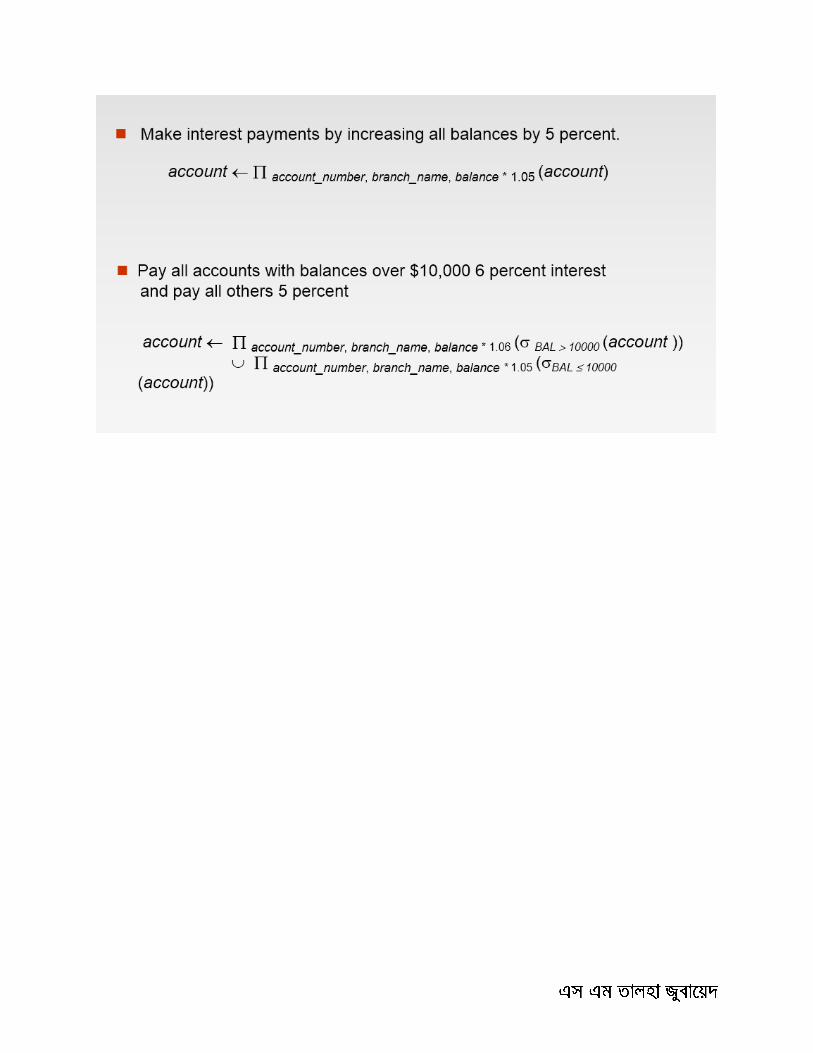
Updates Increase all accounts with balances over $10,000 by 6%, all other accounts
receive 5%.
Write two update statements: update account
set balance = balance 1.06 where balance > 10000
update account
set balance = balance 1.05
where balance 10000
The order is important
Can be done better using the case statement (next slide)
Case Statement for
Conditional Updates Same query as before: Increase all accounts with balances over $10,000 by 6%,
all other accounts receive 5%.
update account set balance = case
when balance <= 10000 then balance *1.05 else balance * 1.06 end
Update of a View Create a view of all loan data in the loan relation, hiding the amount attribute create view loan_branch as
select loan_number, branch_name from loan
Add a new tuple to branch_loan insert into branch_loan
values ('L-37‘, 'Perryridge‘) This insertion must be represented by the insertion of the tuple ('L-37', 'Perryridge', null ) into the loan relation
Some updates through views are impossible to translate into updates on the database relations
create view v as select loan_number, branch_name, amount from loan where branch_name = ‘Perryridge’
insert into v values ( 'L-99','Downtown', '23')
Others cannot be translated uniquely
insert into all_customer values ('Perryridge', 'John') Have to choose loan or account, and
create a new loan/account number!
Most SQL implementations allow updates only on simple views (without aggregates) defined on a single relation
Joined Relations** Join operations take two relations and return as a result another relation.
These additional operations are typically used as subquery expressions in the from clause
Join condition – defines which tuples in the two relations match, and what attributes are present in the result of the join.
Join type – defines how tuples in each relation that do not match any tuple in the other relation (based on the join condition) are treated.
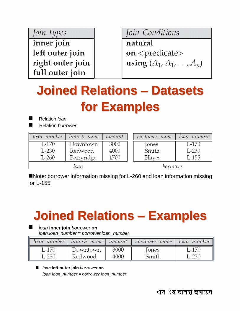
Joined Relations – Datasets
for Examples Relation loan
Relation borrower
Note: borrower information missing for L-260 and loan information missing
for L-155
Joined Relations – Examples loan inner join borrower on
loan.loan_number = borrower.loan_number
loan left outer join borrower on
loan.loan_number = borrower.loan_number
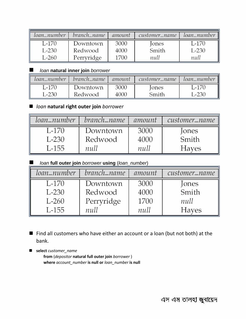
loan natural inner join borrower
loan natural right outer join borrower
loan full outer join borrower using (loan_number)
Find all customers who have either an account or a loan (but not both) at the
bank.
select customer_name
from (depositor natural full outer join borrower )
where account_number is null or loan_number is null

2014
11/16/2014

Entity-Relationship Model Entity Sets Relationship Sets Design Issues Mapping Constraints Keys E-R Diagram Extended E-R Features Design of an E-R Database Schema Reduction of an E-R Schema to Tables
Entity Sets A database can be modeled as:
a collection of entities,
relationship among entities.
An entity is an object that exists and is distinguishable from other objects. Example: specific person, company, event,
plant Entities have attributes
Example: people have names and addresses
An entity set is a set of entities of the same type that share the same properties. Example: set of all persons, companies, trees, holidays
Entity Sets customer and loan
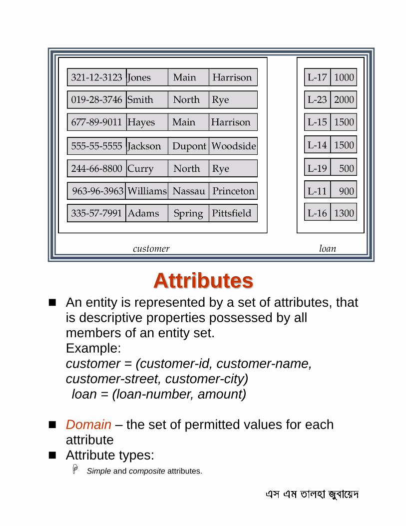
Attributes An entity is represented by a set of attributes, that
is descriptive properties possessed by all members of an entity set.
Example: customer = (customer-id, customer-name,
customer-street, customer-city) loan = (loan-number, amount)
Domain – the set of permitted values for each
attribute Attribute types:
Simple and composite attributes.

Single-valued and multi-valued attributes
E.g. multivalued attribute: phone-numbers
Derived attributes
Can be computed from other attributes
E.g. age, given date of birth
Composite Attributes
Relationship Sets A relationship is an association among several
entities Example:
Hayes depositor A-102 customer entity relationship set account entity
A relationship set is a mathematical relation
among n 2 entities, each taken from entity sets {(e1, e2, … en) | e1 E1, e2 E2, …, en
En} where (e1, e2, …, en) is a relationship Example: (Hayes, A-102) depositor
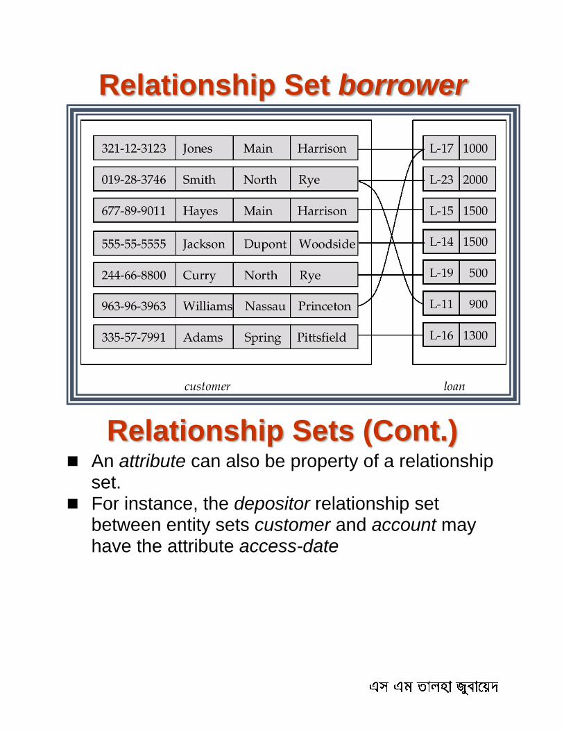
Relationship Set borrower
Relationship Sets (Cont.) An attribute can also be property of a relationship
set. For instance, the depositor relationship set
between entity sets customer and account may have the attribute access-date
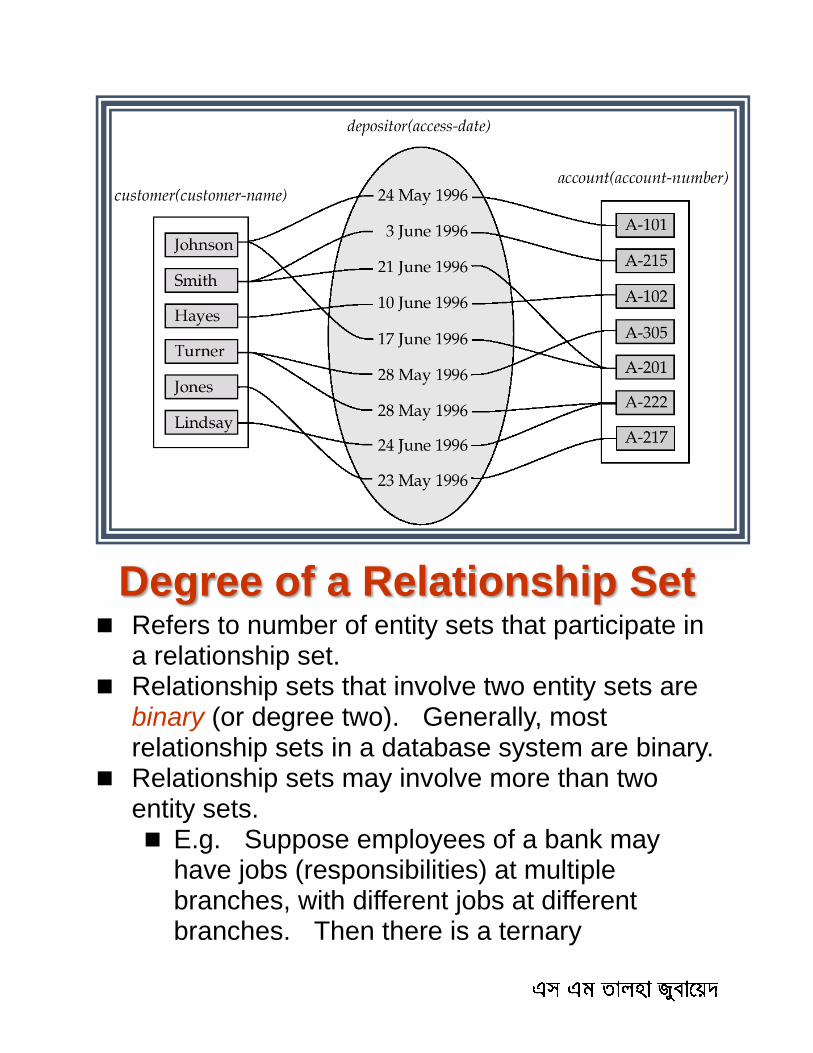
Degree of a Relationship Set Refers to number of entity sets that participate in
a relationship set. Relationship sets that involve two entity sets are
binary (or degree two). Generally, most relationship sets in a database system are binary.
Relationship sets may involve more than two entity sets. E.g. Suppose employees of a bank may
have jobs (responsibilities) at multiple branches, with different jobs at different branches. Then there is a ternary
relationship set between entity sets employee, job and branch
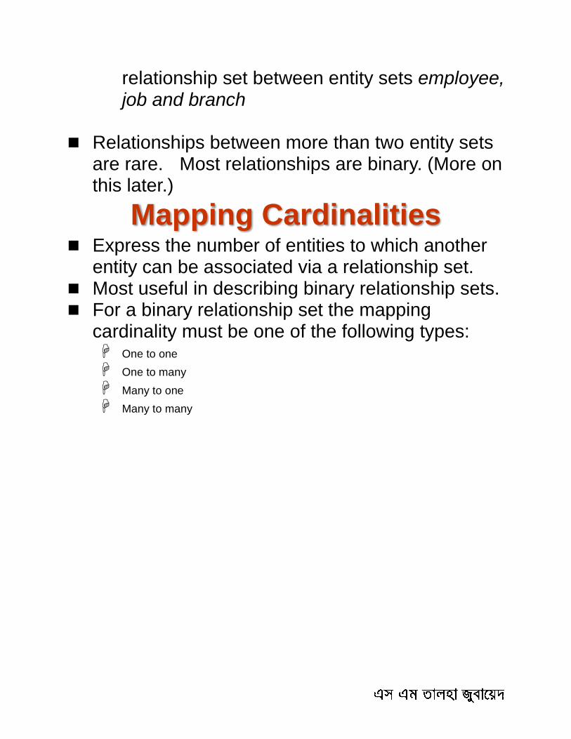
Relationships between more than two entity sets
are rare. Most relationships are binary. (More on this later.)
Mapping Cardinalities Express the number of entities to which another
entity can be associated via a relationship set. Most useful in describing binary relationship sets. For a binary relationship set the mapping
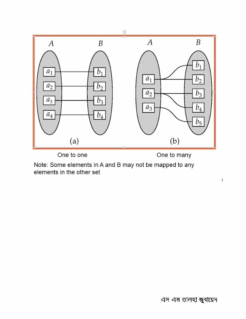
cardinality must be one of the following types: One to one
One to many
Many to one
Many to many
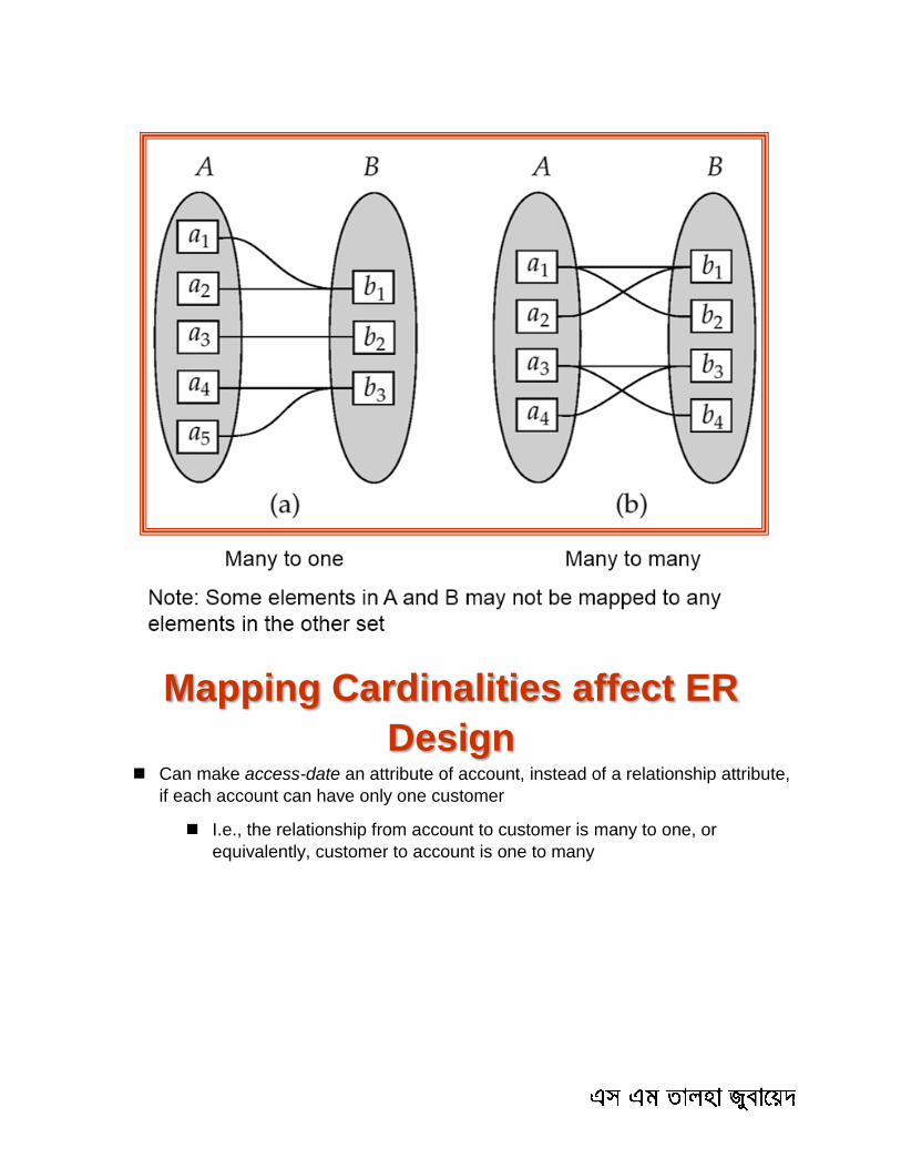
Mapping Cardinalities affect ER
Design Can make access-date an attribute of account, instead of a relationship attribute,
if each account can have only one customer
I.e., the relationship from account to customer is many to one, or
equivalently, customer to account is one to many
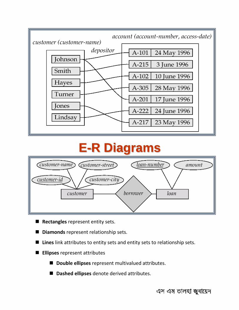
E-R Diagrams
Rectangles represent entity sets.
Diamonds represent relationship sets.
Lines link attributes to entity sets and entity sets to relationship sets.
Ellipses represent attributes
Double ellipses represent multivalued attributes.
Dashed ellipses denote derived attributes.
Underline indicates primary key attributes (will study later)
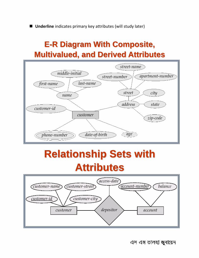
E-R Diagram With Composite,
Multivalued, and Derived Attributes
Relationship Sets with
Attributes
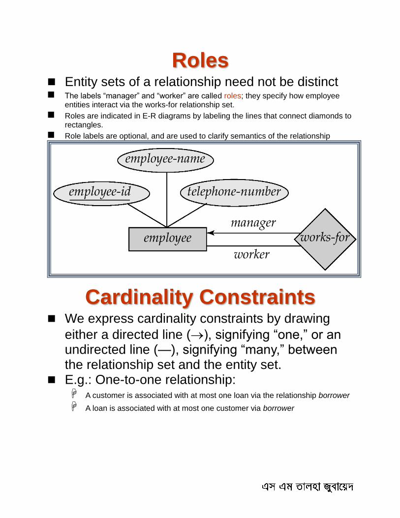
Roles Entity sets of a relationship need not be distinct
The labels “manager” and “worker” are called roles; they specify how employee entities interact via the works-for relationship set.
Roles are indicated in E-R diagrams by labeling the lines that connect diamonds to rectangles.
Role labels are optional, and are used to clarify semantics of the relationship
Cardinality Constraints We express cardinality constraints by drawing
either a directed line (), signifying “one,” or an undirected line (—), signifying “many,” between the relationship set and the entity set.
E.g.: One-to-one relationship: A customer is associated with at most one loan via the relationship borrower
A loan is associated with at most one customer via borrower
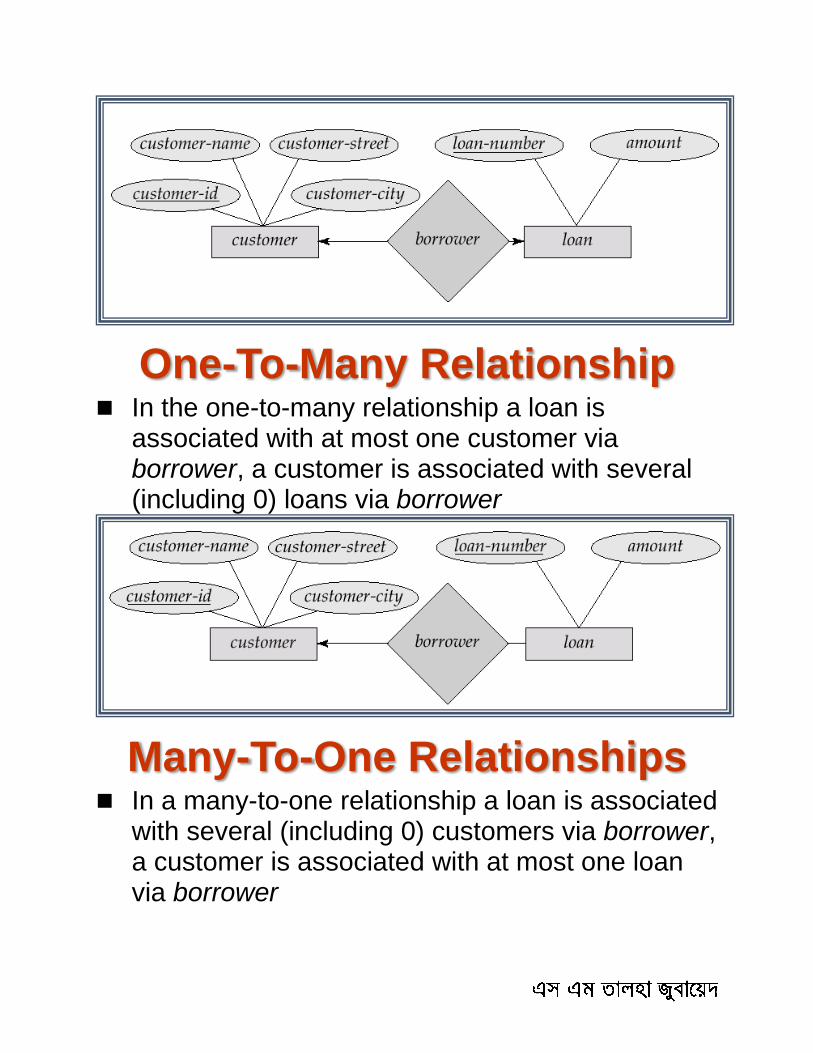
One-To-Many Relationship In the one-to-many relationship a loan is
associated with at most one customer via borrower, a customer is associated with several (including 0) loans via borrower
Many-To-One Relationships In a many-to-one relationship a loan is associated
with several (including 0) customers via borrower, a customer is associated with at most one loan via borrower
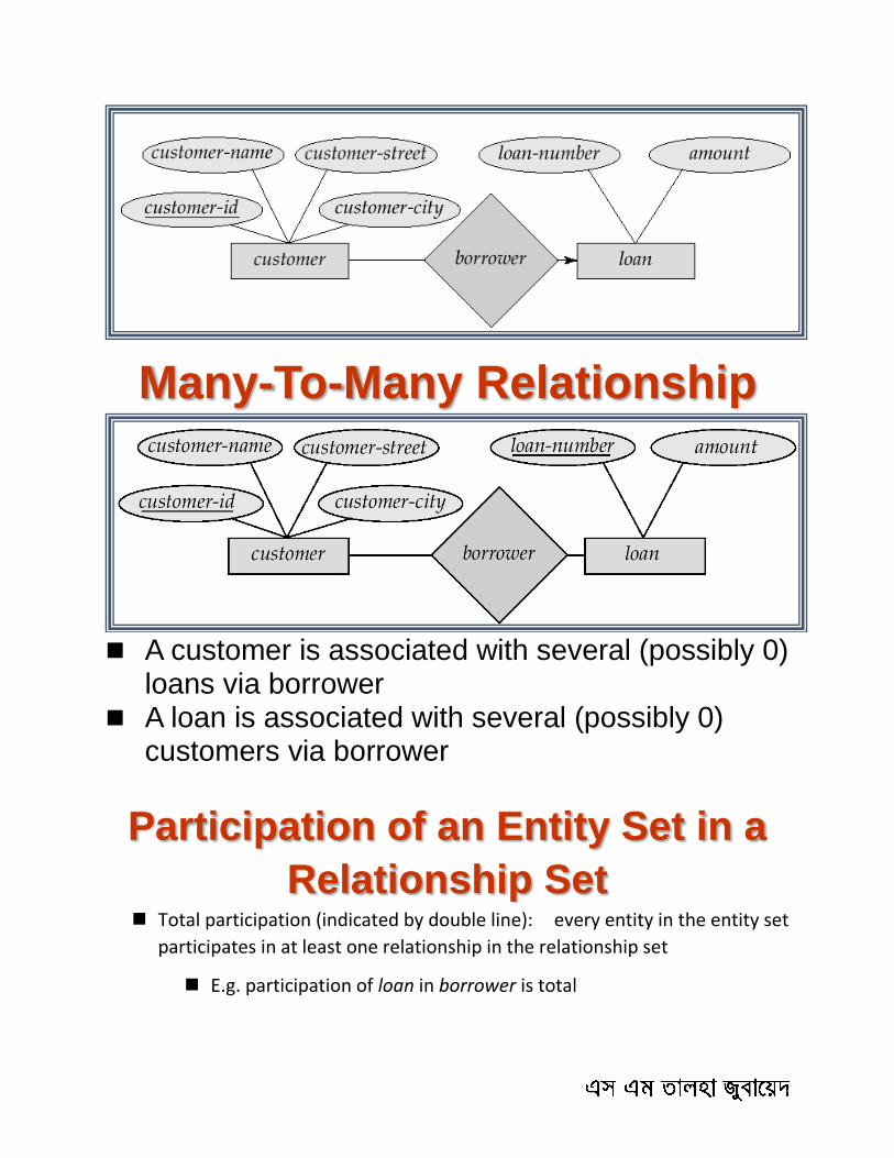
Many-To-Many Relationship
A customer is associated with several (possibly 0)
loans via borrower A loan is associated with several (possibly 0)
customers via borrower
Participation of an Entity Set in a
Relationship Set Total participation (indicated by double line): every entity in the entity set
participates in at least one relationship in the relationship set
E.g. participation of loan in borrower is total
every loan must have a customer associated to it via
borrower
Partial participation: some entities may not participate in any relationship
in the relationship set
E.g. participation of customer in borrower is partial
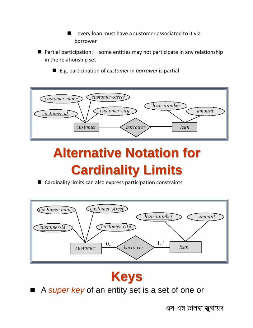
Alternative Notation for
Cardinality Limits Cardinality limits can also express participation constraints
Keys A super key of an entity set is a set of one or
more attributes whose values uniquely determine each entity.
A candidate key of an entity set is a minimal super key Customer-id is candidate key of customer
account-number is candidate key of account
Although several candidate keys may exist, one of the candidate keys is selected to be the primary key.
Keys for Relationship Sets The combination of primary keys of the
participating entity sets forms a super key of a relationship set. (customer-id, account-number) is the super key of depositor
NOTE: this means a pair of entity sets can have at most one relationship in a particular relationship set.
E.g. if we wish to track all access-dates to each account by each customer, we cannot assume a relationship for each access. We can use a multivalued attribute though
Must consider the mapping cardinality of the relationship set when deciding the what are the candidate keys
Need to consider semantics of relationship set in selecting the primary key in case of more than one candidate key
E-R Diagram with a Ternary
Relationship
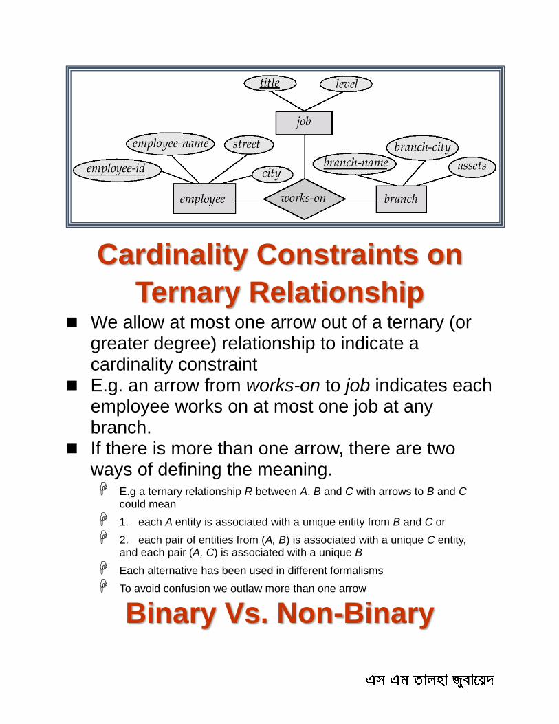
Cardinality Constraints on
Ternary Relationship We allow at most one arrow out of a ternary (or
greater degree) relationship to indicate a cardinality constraint
E.g. an arrow from works-on to job indicates each employee works on at most one job at any branch.
If there is more than one arrow, there are two ways of defining the meaning. E.g a ternary relationship R between A, B and C with arrows to B and C
could mean
1. each A entity is associated with a unique entity from B and C or
2. each pair of entities from (A, B) is associated with a unique C entity, and each pair (A, C) is associated with a unique B
Each alternative has been used in different formalisms
To avoid confusion we outlaw more than one arrow
Binary Vs. Non-Binary
Relationships Some relationships that appear to be non-binary
may be better represented using binary relationships E.g. A ternary relationship parents, relating a child to his/her father and
mother, is best replaced by two binary relationships, father and mother
Using two binary relationships allows partial information (e.g. only mother being know)
But there are some relationships that are naturally non-binary
E.g. works-on
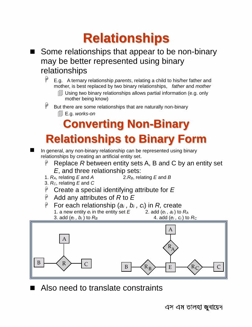
Converting Non-Binary
Relationships to Binary Form In general, any non-binary relationship can be represented using binary
relationships by creating an artificial entity set.
Replace R between entity sets A, B and C by an entity set E, and three relationship sets:
1. RA, relating E and A 2.RB, relating E and B 3. RC, relating E and C
Create a special identifying attribute for E
Add any attributes of R to E
For each relationship (ai , bi , ci) in R, create 1. a new entity ei in the entity set E 2. add (ei , ai ) to RA
3. add (ei , bi ) to RB 4. add (ei , ci ) to RC
Also need to translate constraints
Translating all constraints may not be possible
There may be instances in the translated schema that cannot correspond to any instance of R
Exercise: add constraints to the relationships RA, RB and RC to ensure that a newly created entity corresponds to exactly one entity in each of entity sets A, B and C
We can avoid creating an identifying attribute by making E a weak entity set (described shortly) identified by the three relationship sets
Design Issues Use of entity sets vs. attributes
Choice mainly depends on the structure of the enterprise being modeled, and on the semantics associated with the attribute in question.
Use of entity sets vs. relationship sets Possible guideline is to designate a relationship set to describe an action that occurs between entities
Binary versus n-ary relationship sets Although it is possible to replace any nonbinary (n-ary, for n > 2) relationship set by a number of distinct binary relationship sets, a n-ary relationship set shows more clearly that several entities participate in a single relationship.
Placement of relationship attributes
How about doing an ER design interactively on
the board?
Suggest an application to be modeled.
Specialization Top-down design process; we designate
subgroupings within an entity set that are distinctive from other entities in the set.
These subgroupings become lower-level entity sets that have attributes or participate in relationships that do not apply to the higher-level entity set.
Depicted by a triangle component labeled ISA (E.g. customer “is a” person).
Attribute inheritance – a lower-level entity set inherits all the attributes and relationship participation of the higher-level entity set to which it is linked.
Specialization Example
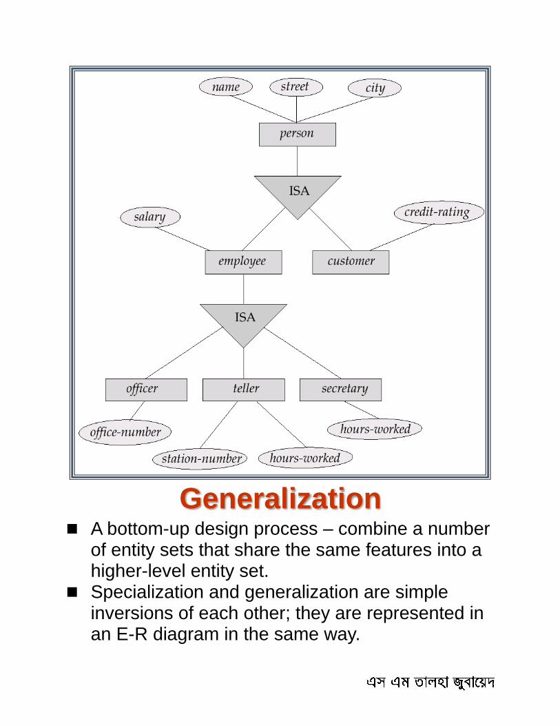
Generalization
A bottom-up design process – combine a number of entity sets that share the same features into a higher-level entity set.
Specialization and generalization are simple inversions of each other; they are represented in an E-R diagram in the same way.

The terms specialization and generalization are used interchangeably.
Specialization and
Generalization (Contd.) Can have multiple specializations of an entity set
based on different features. E.g. permanent-employee vs. temporary-
employee, in addition to officer vs. secretary vs. teller
Each particular employee would be a member of one of permanent-employee or temporary-employee,
and also a member of one of officer, secretary, or teller
The ISA relationship also referred to as superclass - subclass relationship
Design Constraints on a
Specialization/Generalization Constraint on which entities can be members of a
given lower-level entity set. condition-defined
E.g. all customers over 65 years are members of senior-citizen entity set; senior-citizen ISA person.
user-defined
Constraint on whether or not entities may belong to more than one lower-level entity set within a single generalization. Disjoint
an entity can belong to only one lower-level entity set
Noted in E-R diagram by writing disjoint next to the ISA triangle
Overlapping
an entity can belong to more than one lower-level entity set
Design Constraints on a
Specialization/Generalization
(Contd.) Completeness constraint -- specifies whether or
not an entity in the higher-level entity set must belong to at least one of the lower-level entity sets within a generalization. total : an entity must belong to one of the lower-level entity sets
partial: an entity need not belong to one of the lower-level entity sets
E-R Design Decisions The use of an attribute or entity set to represent
an object. Whether a real-world concept is best expressed
by an entity set or a relationship set. The use of a ternary relationship versus a pair of
binary relationships. The use of specialization/generalization –
contributes to modularity in the design.
E-R Diagram for a Banking
Enterprise

How about doing another ER design
interactively on the board?

Summary of Symbols Used in
E-R Notation
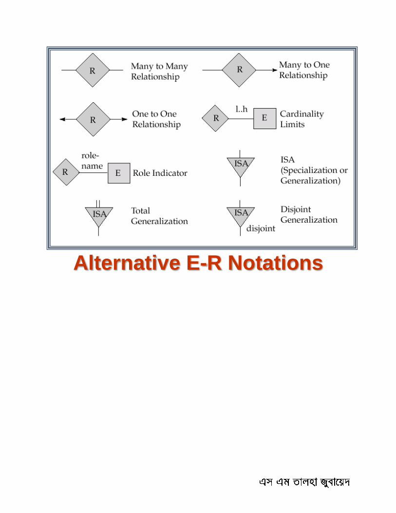
Alternative E-R Notations
UML UML: Unified Modeling Language UML has many components to graphically model
different aspects of an entire software system UML Class Diagrams correspond to E-R
Diagram, but several differences.
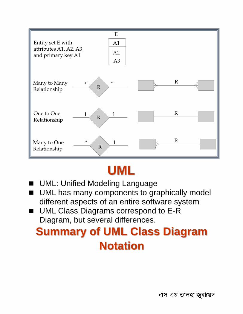
Summary of UML Class Diagram
Notation
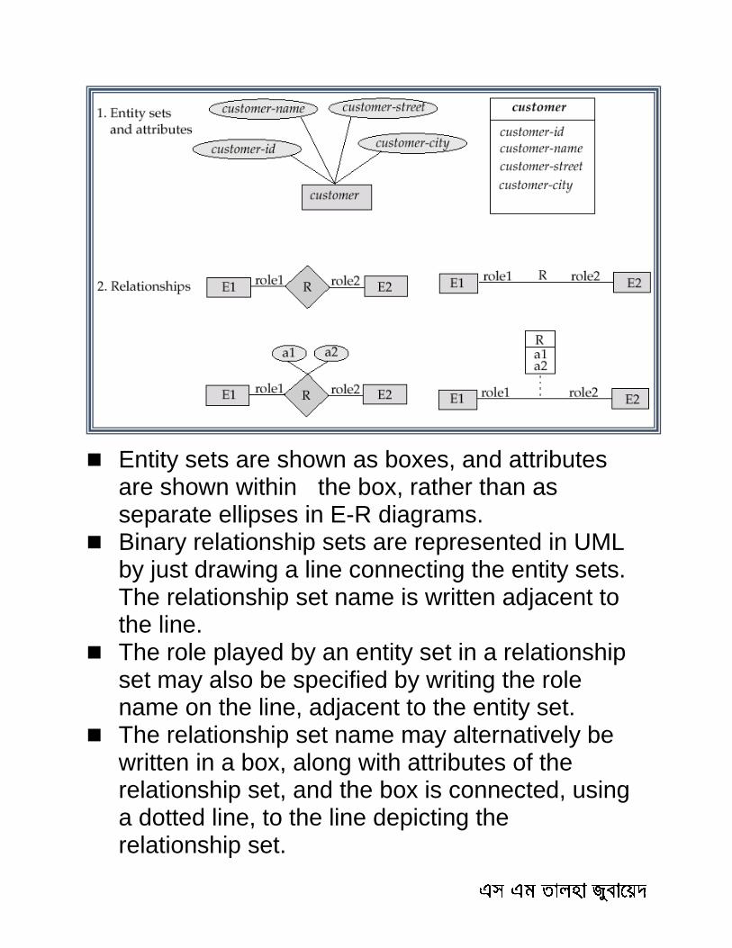
Entity sets are shown as boxes, and attributes are shown within the box, rather than as separate ellipses in E-R diagrams.
Binary relationship sets are represented in UML by just drawing a line connecting the entity sets. The relationship set name is written adjacent to the line.
The role played by an entity set in a relationship set may also be specified by writing the role name on the line, adjacent to the entity set.
The relationship set name may alternatively be written in a box, along with attributes of the relationship set, and the box is connected, using a dotted line, to the line depicting the relationship set.
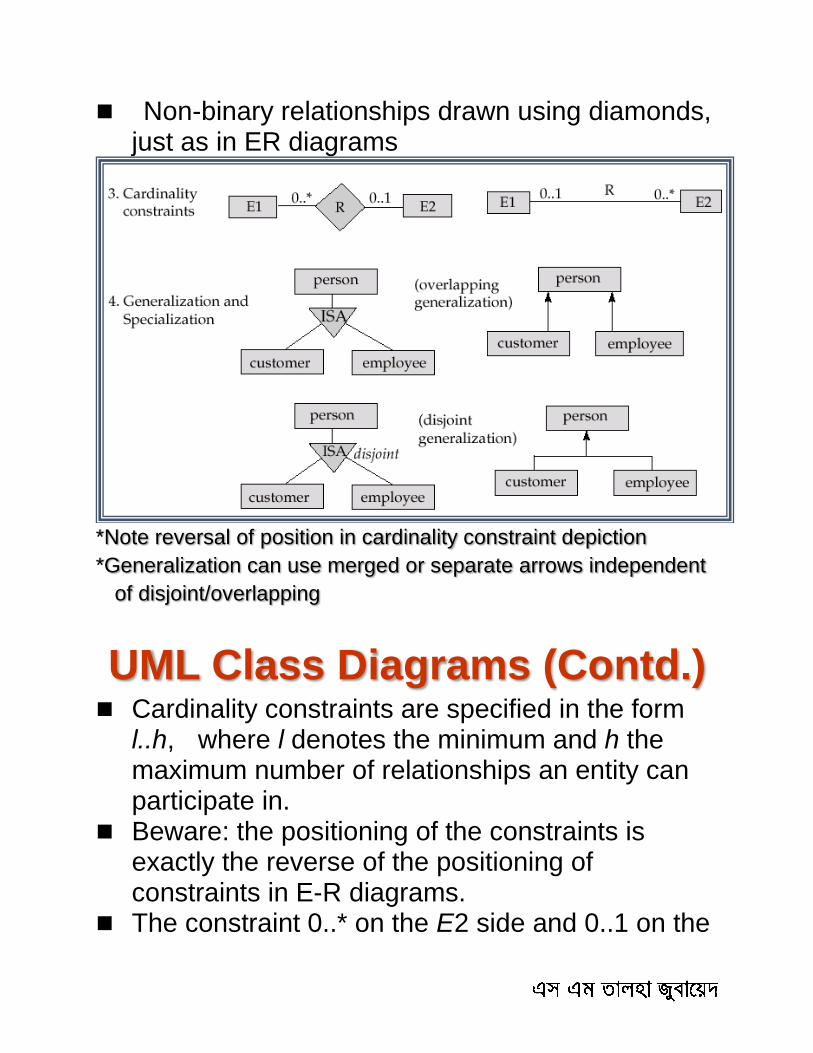
Non-binary relationships drawn using diamonds, just as in ER diagrams
*Note reversal of position in cardinality constraint depiction
*Generalization can use merged or separate arrows independent
of disjoint/overlapping
UML Class Diagrams (Contd.) Cardinality constraints are specified in the form
l..h, where l denotes the minimum and h the maximum number of relationships an entity can participate in.
Beware: the positioning of the constraints is exactly the reverse of the positioning of constraints in E-R diagrams.
The constraint 0..* on the E2 side and 0..1 on the

E1 side means that each E2 entity can participate in at most one relationship, whereas each E1 entity can participate in many relationships; in other words, the relationship is many to one from E2 to E1.
Single values, such as 1 or * may be written on edges; The single value 1 on an edge is treated as equivalent to 1..1, while * is equivalent to 0..*.
Reduction of an E-R Schema
to Tables Primary keys allow entity sets and relationship
sets to be expressed uniformly as tables which represent the contents of the database.
A database which conforms to an E-R diagram can be represented by a collection of tables.
For each entity set and relationship set there is a unique table which is assigned the name of the corresponding entity set or relationship set.
Each table has a number of columns (generally corresponding to attributes), which have unique names.
Converting an E-R diagram to a table format is the basis for deriving a relational database design from an E-R diagram.
Representing Entity Sets as
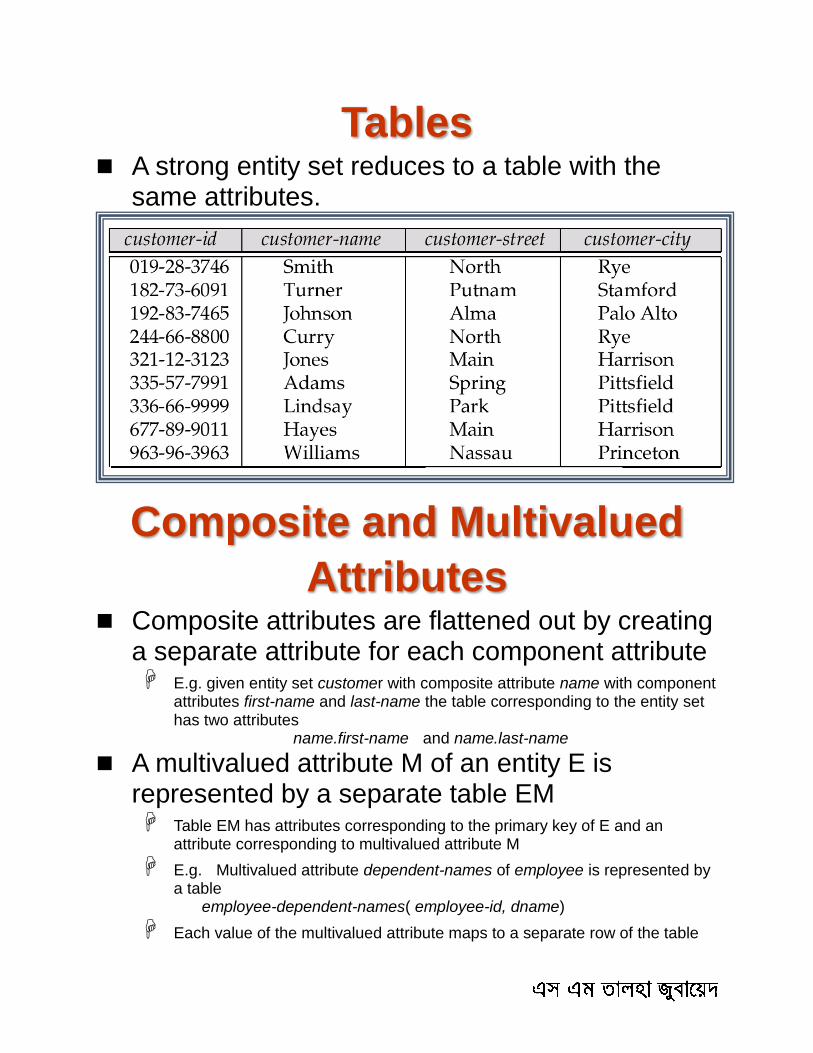
Tables A strong entity set reduces to a table with the
same attributes.
Composite and Multivalued
Attributes Composite attributes are flattened out by creating
a separate attribute for each component attribute E.g. given entity set customer with composite attribute name with component
attributes first-name and last-name the table corresponding to the entity set has two attributes name.first-name and name.last-name
A multivalued attribute M of an entity E is represented by a separate table EM Table EM has attributes corresponding to the primary key of E and an
attribute corresponding to multivalued attribute M
E.g. Multivalued attribute dependent-names of employee is represented by a table employee-dependent-names( employee-id, dname)
Each value of the multivalued attribute maps to a separate row of the table
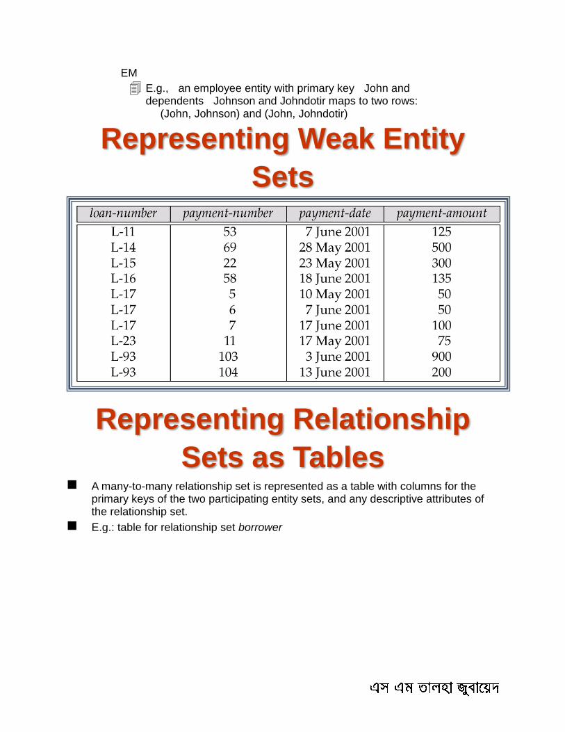
EM
E.g., an employee entity with primary key John and dependents Johnson and Johndotir maps to two rows: (John, Johnson) and (John, Johndotir)
Representing Weak Entity
Sets
Representing Relationship
Sets as Tables A many-to-many relationship set is represented as a table with columns for the
primary keys of the two participating entity sets, and any descriptive attributes of the relationship set.
E.g.: table for relationship set borrower
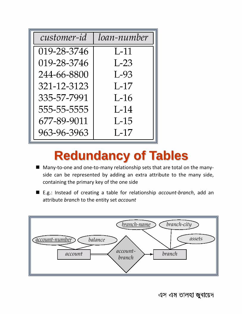
Redundancy of Tables Many-to-one and one-to-many relationship sets that are total on the many-
side can be represented by adding an extra attribute to the many side,
containing the primary key of the one side
E.g.: Instead of creating a table for relationship account-branch, add an
attribute branch to the entity set account

For one-to-one relationship sets, either side can be chosen to act as the “many” side That is, extra attribute can be added to either of the tables corresponding to
the two entity sets
If participation is partial on the many side, replacing a table by an extra attribute in the relation corresponding to the “many” side could result in null values
The table corresponding to a relationship set linking a weak entity set to its identifying strong entity set is redundant. E.g. The payment table already contains the information that would appear in
the loan-payment table (i.e., the columns loan-number and payment-number).
Representing Specialization
as Tables Method 1:
Form a table for the higher level entity Form a table for each lower level entity set,
include primary key of higher level entity set and local attributes
table table attributes
person name, street, city
customer name, credit-rating
employee name, salary
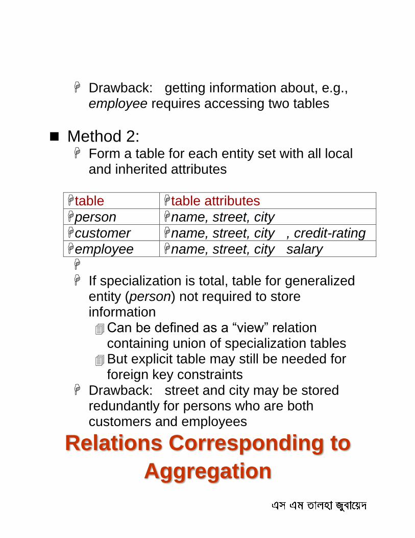
Drawback: getting information about, e.g., employee requires accessing two tables
Method 2: Form a table for each entity set with all local
and inherited attributes
table table attributes
person name, street, city
customer name, street, city , credit-rating
employee name, street, city salary If specialization is total, table for generalized
entity (person) not required to store information Can be defined as a “view” relation
containing union of specialization tables But explicit table may still be needed for
foreign key constraints Drawback: street and city may be stored
redundantly for persons who are both customers and employees
Relations Corresponding to
Aggregation

2014
11/16/2014
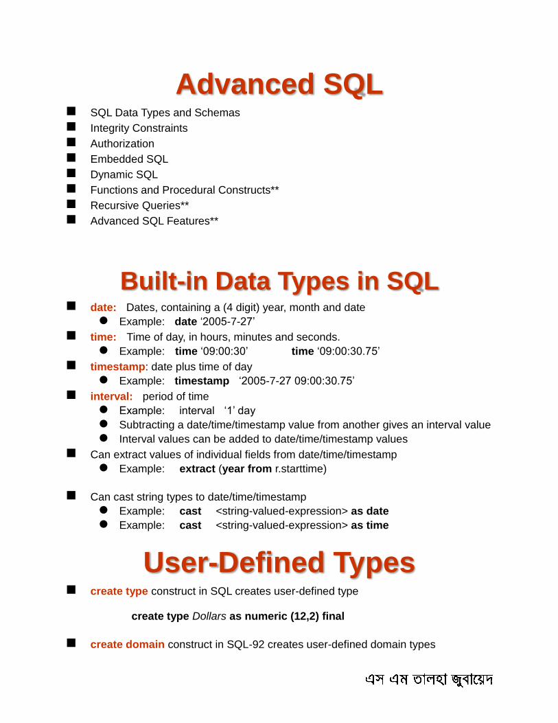
Advanced SQL SQL Data Types and Schemas
Integrity Constraints
Authorization
Embedded SQL
Dynamic SQL
Functions and Procedural Constructs**
Recursive Queries**
Advanced SQL Features**
Built-in Data Types in SQL date: Dates, containing a (4 digit) year, month and date
Example: date ‘2005-7-27’
time: Time of day, in hours, minutes and seconds.
Example: time ‘09:00:30’ time ‘09:00:30.75’
timestamp: date plus time of day
Example: timestamp ‘2005-7-27 09:00:30.75’
interval: period of time
Example: interval ‘1’ day
Subtracting a date/time/timestamp value from another gives an interval value
Interval values can be added to date/time/timestamp values
Can extract values of individual fields from date/time/timestamp
Example: extract (year from r.starttime)
Can cast string types to date/time/timestamp
Example: cast <string-valued-expression> as date
Example: cast <string-valued-expression> as time
User-Defined Types create type construct in SQL creates user-defined type
create type Dollars as numeric (12,2) final
create domain construct in SQL-92 creates user-defined domain types
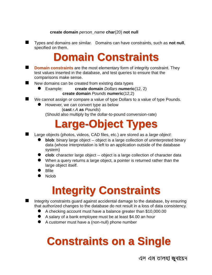
create domain person_name char(20) not null
Types and domains are similar. Domains can have constraints, such as not null, specified on them.
Domain Constraints Domain constraints are the most elementary form of integrity constraint. They
test values inserted in the database, and test queries to ensure that the comparisons make sense.
New domains can be created from existing data types
Example: create domain Dollars numeric(12, 2) create domain Pounds numeric(12,2)
We cannot assign or compare a value of type Dollars to a value of type Pounds.
However, we can convert type as below (cast r.A as Pounds) (Should also multiply by the dollar-to-pound conversion-rate)
Large-Object Types Large objects (photos, videos, CAD files, etc.) are stored as a large object:
blob: binary large object -- object is a large collection of uninterpreted binary data (whose interpretation is left to an application outside of the database system)
clob: character large object -- object is a large collection of character data
When a query returns a large object, a pointer is returned rather than the large object itself.
Bfile
Nclob
Integrity Constraints Integrity constraints guard against accidental damage to the database, by ensuring
that authorized changes to the database do not result in a loss of data consistency.
A checking account must have a balance greater than $10,000.00
A salary of a bank employee must be at least $4.00 an hour
A customer must have a (non-null) phone number
Constraints on a Single
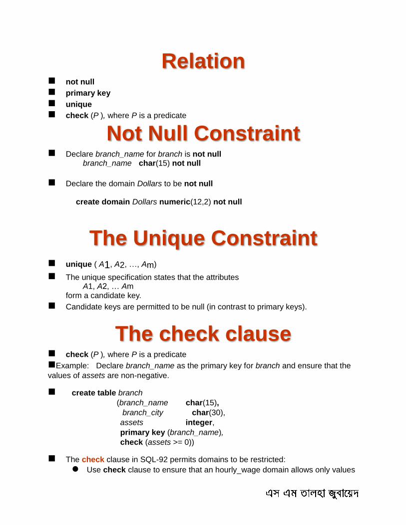
Relation not null
primary key
unique
check (P ), where P is a predicate
Not Null Constraint Declare branch_name for branch is not null branch_name char(15) not null
Declare the domain Dollars to be not null create domain Dollars numeric(12,2) not null
The Unique Constraint unique ( A1, A2, …, Am)
The unique specification states that the attributes A1, A2, … Am
form a candidate key.
Candidate keys are permitted to be null (in contrast to primary keys).
The check clause check (P ), where P is a predicate
Example: Declare branch_name as the primary key for branch and ensure that the
values of assets are non-negative.
create table branch
(branch_name char(15),
branch_city char(30),
assets integer,
primary key (branch_name),
check (assets >= 0))
The check clause in SQL-92 permits domains to be restricted:
Use check clause to ensure that an hourly_wage domain allows only values
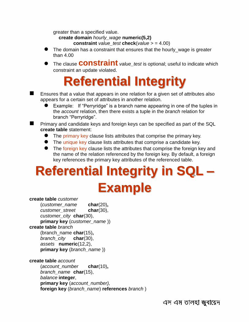
greater than a specified value. create domain hourly_wage numeric(5,2)
constraint value_test check(value > = 4.00)
The domain has a constraint that ensures that the hourly_wage is greater than 4.00
The clause constraint value_test is optional; useful to indicate which
constraint an update violated.
Referential Integrity Ensures that a value that appears in one relation for a given set of attributes also
appears for a certain set of attributes in another relation.
Example: If “Perryridge” is a branch name appearing in one of the tuples in the account relation, then there exists a tuple in the branch relation for branch “Perryridge”.
Primary and candidate keys and foreign keys can be specified as part of the SQL create table statement:
The primary key clause lists attributes that comprise the primary key.
The unique key clause lists attributes that comprise a candidate key.
The foreign key clause lists the attributes that comprise the foreign key and the name of the relation referenced by the foreign key. By default, a foreign key references the primary key attributes of the referenced table.
Referential Integrity in SQL –
Example create table customer
(customer_name char(20), customer_street char(30), customer_city char(30), primary key (customer_name ))
create table branch (branch_name char(15), branch_city char(30), assets numeric(12,2), primary key (branch_name ))
create table account
(account_number char(10), branch_name char(15), balance integer, primary key (account_number), foreign key (branch_name) references branch )
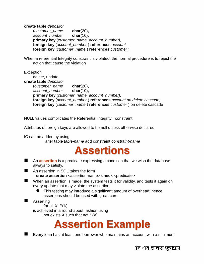
create table depositor (customer_name char(20), account_number char(10), primary key (customer_name, account_number), foreign key (account_number ) references account, foreign key (customer_name ) references customer )
When a referential Integrity constraint is violated, the normal procedure is to reject the
action that cause the violation Exception delete, update create table depositor
(customer_name char(20), account_number char(10), primary key (customer_name, account_number), foreign key (account_number ) references account on delete cascade, foreign key (customer_name ) references customer ) on delete cascade
NULL values complicates the Referential Integrity constraint Attributes of foreign keys are allowed to be null unless otherwise declared IC can be added by using alter table table-name add constraint constraint-name
Assertions An assertion is a predicate expressing a condition that we wish the database
always to satisfy.
An assertion in SQL takes the form create assertion <assertion-name> check <predicate>
When an assertion is made, the system tests it for validity, and tests it again on every update that may violate the assertion
This testing may introduce a significant amount of overhead; hence assertions should be used with great care.
Asserting for all X, P(X) is achieved in a round-about fashion using not exists X such that not P(X)
Assertion Example Every loan has at least one borrower who maintains an account with a minimum
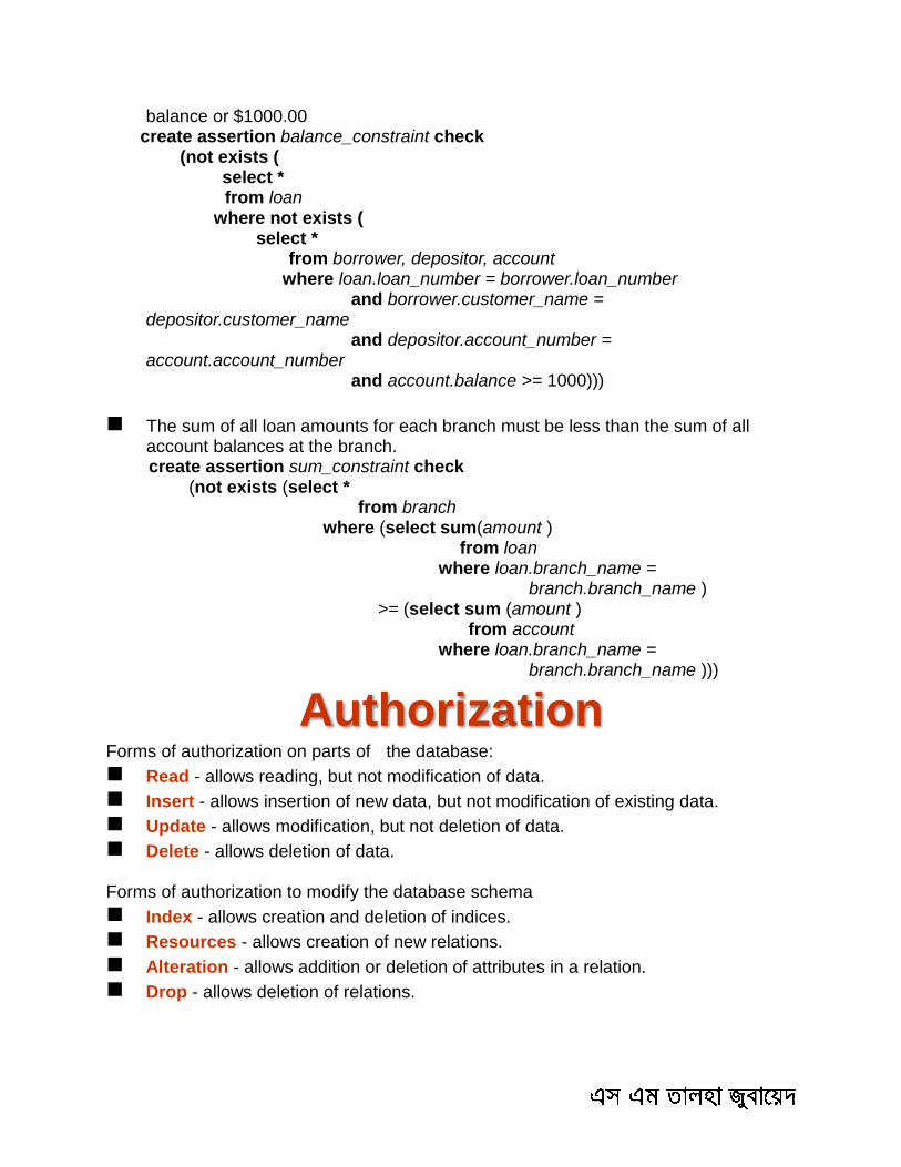
balance or $1000.00 create assertion balance_constraint check
(not exists ( select *
from loan where not exists ( select * from borrower, depositor, account where loan.loan_number = borrower.loan_number and borrower.customer_name = depositor.customer_name and depositor.account_number = account.account_number and account.balance >= 1000)))
The sum of all loan amounts for each branch must be less than the sum of all account balances at the branch.
create assertion sum_constraint check (not exists (select * from branch where (select sum(amount ) from loan where loan.branch_name = branch.branch_name ) >= (select sum (amount ) from account where loan.branch_name = branch.branch_name )))
Authorization Forms of authorization on parts of the database:
Read - allows reading, but not modification of data.
Insert - allows insertion of new data, but not modification of existing data.
Update - allows modification, but not deletion of data.
Delete - allows deletion of data. Forms of authorization to modify the database schema
Index - allows creation and deletion of indices.
Resources - allows creation of new relations.
Alteration - allows addition or deletion of attributes in a relation.
Drop - allows deletion of relations.
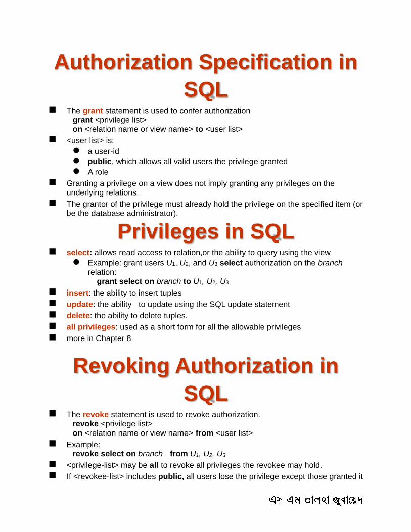
Authorization Specification in
SQL The grant statement is used to confer authorization grant <privilege list> on <relation name or view name> to <user list>
<user list> is:
a user-id
public, which allows all valid users the privilege granted
A role
Granting a privilege on a view does not imply granting any privileges on the underlying relations.
The grantor of the privilege must already hold the privilege on the specified item (or be the database administrator).
Privileges in SQL select: allows read access to relation,or the ability to query using the view
Example: grant users U1, U2, and U3 select authorization on the branch relation:
grant select on branch to U1, U2, U3
insert: the ability to insert tuples
update: the ability to update using the SQL update statement
delete: the ability to delete tuples.
all privileges: used as a short form for all the allowable privileges
more in Chapter 8
Revoking Authorization in
SQL The revoke statement is used to revoke authorization.
revoke <privilege list> on <relation name or view name> from <user list>
Example: revoke select on branch from U1, U2, U3
<privilege-list> may be all to revoke all privileges the revokee may hold.
If <revokee-list> includes public, all users lose the privilege except those granted it
explicitly.
If the same privilege was granted twice to the same user by different grantees, the user may retain the privilege after the revocation.
All privileges that depend on the privilege being revoked are also revoked.
Embedded SQL The SQL standard defines embeddings of SQL in a variety of programming
languages such as C, Java, and Cobol.
A language to which SQL queries are embedded is referred to as a host language, and the SQL structures permitted in the host language comprise embedded SQL.
The basic form of these languages follows that of the System R embedding of SQL into PL/I.
EXEC SQL statement is used to identify embedded SQL request to the preprocessor
EXEC SQL <embedded SQL statement > END_EXEC Note: this varies by language (for example, the Java embedding uses
# SQL { …. }; )
Example Query Specify the query in SQL and declare a cursor for it EXEC SQL declare c cursor for
select depositor.customer_name, customer_city from depositor, customer, account where depositor.customer_name = customer.customer_name and depositor account_number = account.account_number and account.balance > :amount
END_EXEC
The open statement causes the query to be evaluated EXEC SQL open c END_EXEC
The fetch statement causes the values of one tuple in the query result to be placed on host language variables.
EXEC SQL fetch c into :cn, :cc END_EXEC Repeated calls to fetch get successive tuples in the query result
A variable called SQLSTATE in the SQL communication area (SQLCA) gets set to ‘02000’ to indicate no more data is available
The close statement causes the database system to delete the temporary relation that holds the result of the query.
EXEC SQL close c END_EXEC

Note: above details vary with language. For example, the Java embedding defines Java iterators to step through result tuples.
Updates Through Cursors Can update tuples fetched by cursor by declaring that the cursor is for update declare c cursor for select * from account where branch_name = ‘Perryridge’ for update To update tuple at the current location of cursor c update account set balance = balance + 100 where current of c
Dynamic SQL Allows programs to construct and submit SQL queries at run time.
Example of the use of dynamic SQL from within a C program. char * sqlprog = “update account set balance = balance * 1.05 where account_number = ?” EXEC SQL prepare dynprog from :sqlprog; char account [10] = “A-101”; EXEC SQL execute dynprog using :account;
The dynamic SQL program contains a ?, which is a place holder for a value that is provided when the SQL program is executed.
JDBC JDBC is a Java API for communicating with database systems supporting SQL
JDBC supports a variety of features for querying and updating data, and for retrieving query results
JDBC also supports metadata retrieval, such as querying about relations present in the database and the names and types of relation attributes
Model for communicating with the database:
Open a connection
Create a “statement” object
Execute queries using the Statement object to send queries and fetch results
Exception mechanism to handle errors
JDBC Code public static void JDBCexample(String dbid, String
userid, String passwd) {
try { Class.forName ("oracle.jdbc.driver.OracleDriver"); Connection conn = DriverManager.getConnection(
"jdbc:oracle:thin:@aura.bell-labs.com:2000:bankdb", userid, passwd);
Statement stmt = conn.createStatement(); … Do Actual Work …. stmt.close(); conn.close(); } catch (SQLException sqle) { System.out.println("SQLException : " + sqle);
}
}
Update to database try { stmt.executeUpdate( "insert into account values
('A-9732', 'Perryridge', 1200)"); } catch (SQLException sqle) { System.out.println("Could not insert tuple. " + sqle); }
Execute query and fetch and print results ResultSet rset = stmt.executeQuery( "select branch_name, avg(balance)
from account group by branch_name");
while (rset.next()) { System.out.println(
rset.getString("branch_name") + " " +
rset.getFloat(2)); }
JDBC Code Details Getting result fields:
rs.getString(“branchname”) and rs.getString(1) equivalent if branchname is the first argument of select result.
Dealing with Null values int a = rs.getInt(“a”); if (rs.wasNull()) Systems.out.println(“Got null value”);
Procedural Extensions and Stored
Procedures SQL provides a module language
Permits definition of procedures in SQL, with if-then-else statements, for and while loops, etc.
more in Chapter 9
Stored Procedures
Can store procedures in the database
then execute them using the call statement
permit external applications to operate on the database without knowing about internal details
Functions and Procedures SQL:1999 supports functions and procedures
Functions/procedures can be written in SQL itself, or in an external programming language
Functions are particularly useful with specialized data types such as images and geometric objects Example: functions to check if polygons overlap, or to compare images
for similarity
Some database systems support table-valued functions, which can return a relation as a result
SQL:1999 also supports a rich set of imperative constructs, including
Loops, if-then-else, assignment
Many databases have proprietary procedural extensions to SQL that differ from
SQL:1999
SQL Functions Define a function that, given the name of a customer, returns the count of the
number of accounts owned by the customer. create function account_count (customer_name varchar(20))
returns integer begin declare a_count integer; select count (* ) into a_count from depositor where depositor.customer_name = customer_name return a_count; end
Find the name and address of each customer that has more than one account. select customer_name, customer_street, customer_city
from customer where account_count (customer_name ) > 1
Table Functions SQL:2003 added functions that return a relation as a result
Example: Return all accounts owned by a given customer create function accounts_of (customer_name char(20) returns table ( account_number char(10),
branch_name char(15) balance numeric(12,2))
return table (select account_number, branch_name, balance from account A where exists ( select * from depositor D where D.customer_name = accounts_of.customer_name and D.account_number = A.account_number ))
Usage select *
from table (accounts_of (‘Smith’))
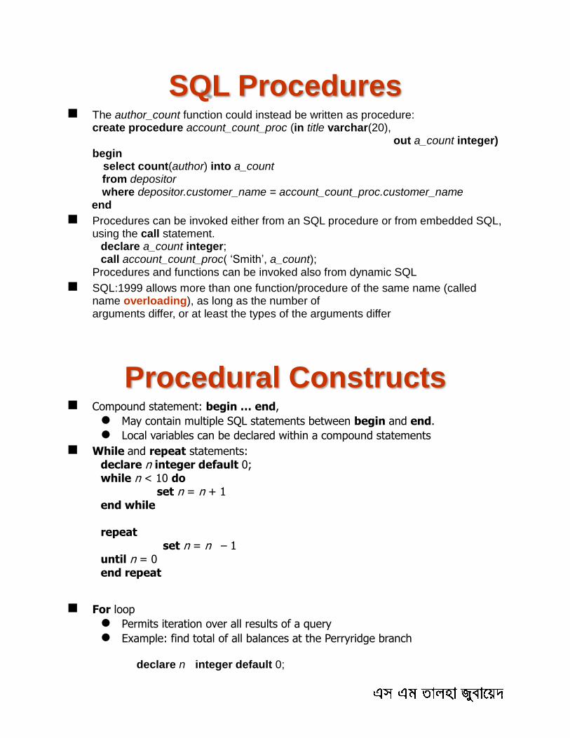
SQL Procedures The author_count function could instead be written as procedure: create procedure account_count_proc (in title varchar(20),
out a_count integer) begin
select count(author) into a_count from depositor where depositor.customer_name = account_count_proc.customer_name
end
Procedures can be invoked either from an SQL procedure or from embedded SQL, using the call statement.
declare a_count integer; call account_count_proc( ‘Smith’, a_count);
Procedures and functions can be invoked also from dynamic SQL
SQL:1999 allows more than one function/procedure of the same name (called name overloading), as long as the number of arguments differ, or at least the types of the arguments differ
Procedural Constructs Compound statement: begin … end,
May contain multiple SQL statements between begin and end.
Local variables can be declared within a compound statements
While and repeat statements: declare n integer default 0; while n < 10 do
set n = n + 1 end while
repeat
set n = n – 1 until n = 0 end repeat
For loop
Permits iteration over all results of a query
Example: find total of all balances at the Perryridge branch declare n integer default 0;

for r as select balance from account where branch_name = ‘Perryridge’ do set n = n + r.balance end for
Conditional statements (if-then-else) E.g. To find sum of balances for each of three categories of accounts (with balance <1000, >=1000 and <5000, >= 5000)
if r.balance < 1000 then set l = l + r.balance elseif r.balance < 5000 then set m = m + r.balance else set h = h + r.balance end if
SQL:1999 also supports a case statement similar to C case statement
Signaling of exception conditions, and declaring handlers for exceptions declare out_of_stock condition
declare exit handler for out_of_stock begin … .. signal out-of-stock end
The handler here is exit -- causes enclosing begin..end to be exited
Other actions possible on exception
External Language
Functions/Procedures SQL:1999 permits the use of functions and procedures written in other languages
such as C or C++
Declaring external language procedures and functions
create procedure account_count_proc(in customer_name varchar(20), out count integer) language C external name ’ /usr/avi/bin/account_count_proc’ create function account_count(customer_name varchar(20)) returns integer language C external name ‘/usr/avi/bin/author_count’
External Language Routines
(Cont.) Benefits of external language functions/procedures:
more efficient for many operations, and more expressive power
Drawbacks
Code to implement function may need to be loaded into database system and executed in the database system’s address space risk of accidental corruption of database structures security risk, allowing users access to unauthorized data
There are alternatives, which give good security at the cost of potentially worse performance
Direct execution in the database system’s space is used when efficiency is more important than security
Security with External Language
Routines To deal with security problems
Use sandbox techniques that is use a safe language like Java, which cannot be used to
access/damage other parts of the database code
Or, run external language functions/procedures in a separate process, with no access to the database process’ memory Parameters and results communicated via inter-process communication
Both have performance overheads
Many database systems support both above approaches as well as direct executing in database system address space
Recursion in SQL SQL:1999 permits recursive view definition
Example: find all employee-manager pairs, where the employee reports to the manager directly or indirectly (that is manager’s manager, manager’s manager’s manager, etc.)
with recursive empl (employee_name, manager_name ) as ( select employee_name, manager_name from manager union select manager.employee_name, empl.manager_name from manager, empl where manager.manager_name = empl.employe_name) select * from empl
This example view, empl, is called the transitive closure of the manager relation
The Power of Recursion Recursive views make it possible to write queries, such as transitive closure
queries, that cannot be written without recursion or iteration.
Intuition: Without recursion, a non-recursive non-iterative program can perform only a fixed number of joins of manager with itself This can give only a fixed number of levels of managers Given a program we can construct a database with a greater number of
levels of managers on which the program will not work
Computing transitive closure
The next slide shows a manager relation
Each step of the iterative process constructs an extended version of empl from its recursive definition.
The final result is called the fixed point of the recursive view definition.
Recursive views are required to be monotonic. That is, if we add tuples to manger the view contains all of the tuples it contained before, plus possibly more
Example of Fixed-Point
Computation
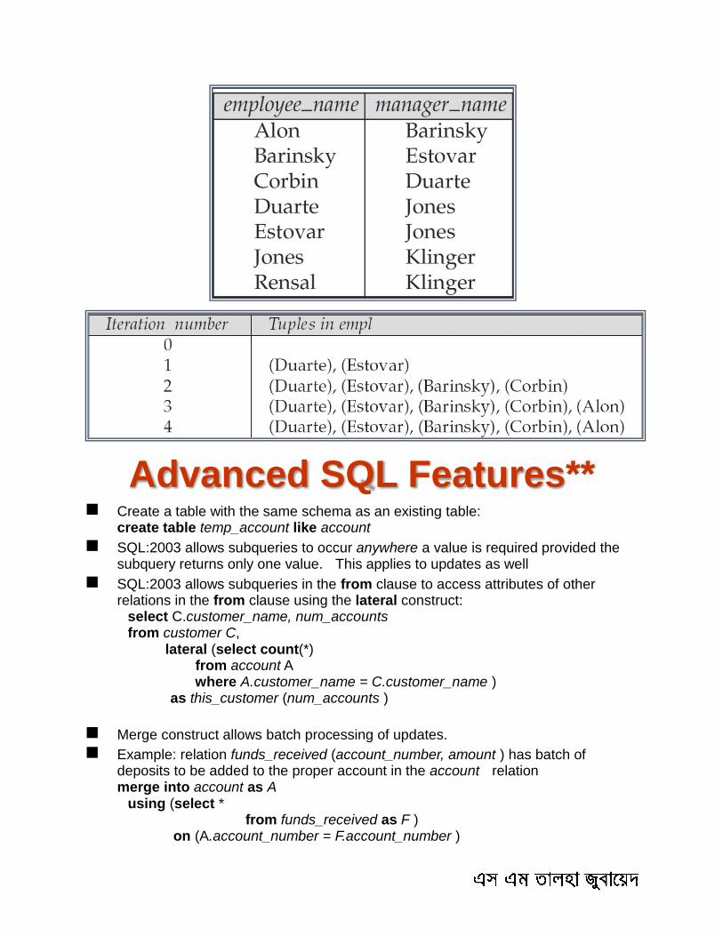
Advanced SQL Features** Create a table with the same schema as an existing table: create table temp_account like account
SQL:2003 allows subqueries to occur anywhere a value is required provided the subquery returns only one value. This applies to updates as well
SQL:2003 allows subqueries in the from clause to access attributes of other relations in the from clause using the lateral construct:
select C.customer_name, num_accounts from customer C, lateral (select count(*) from account A where A.customer_name = C.customer_name ) as this_customer (num_accounts )
Merge construct allows batch processing of updates.
Example: relation funds_received (account_number, amount ) has batch of deposits to be added to the proper account in the account relation
merge into account as A using (select * from funds_received as F ) on (A.account_number = F.account_number )

when matched then update set balance = balance + F.amount

2014
11/16/2014
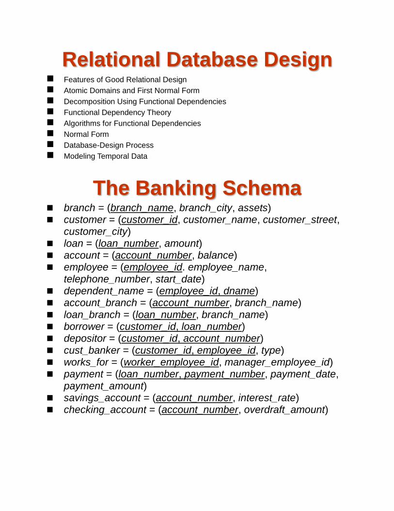
Relational Database Design Features of Good Relational Design
Atomic Domains and First Normal Form
Decomposition Using Functional Dependencies
Functional Dependency Theory
Algorithms for Functional Dependencies
Normal Form
Database-Design Process
Modeling Temporal Data
The Banking Schema branch = (branch_name, branch_city, assets) customer = (customer_id, customer_name, customer_street,
customer_city) loan = (loan_number, amount) account = (account_number, balance) employee = (employee_id. employee_name,
telephone_number, start_date) dependent_name = (employee_id, dname) account_branch = (account_number, branch_name) loan_branch = (loan_number, branch_name) borrower = (customer_id, loan_number) depositor = (customer_id, account_number) cust_banker = (customer_id, employee_id, type) works_for = (worker_employee_id, manager_employee_id) payment = (loan_number, payment_number, payment_date,
payment_amount) savings_account = (account_number, interest_rate) checking_account = (account_number, overdraft_amount)
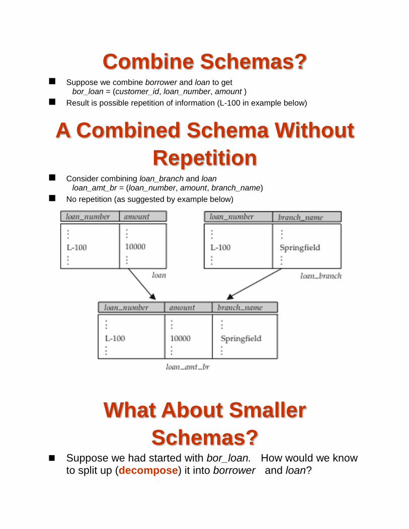
Combine Schemas? Suppose we combine borrower and loan to get
bor_loan = (customer_id, loan_number, amount )
Result is possible repetition of information (L-100 in example below)
A Combined Schema Without
Repetition Consider combining loan_branch and loan
loan_amt_br = (loan_number, amount, branch_name)
No repetition (as suggested by example below)
What About Smaller
Schemas? Suppose we had started with bor_loan. How would we know
to split up (decompose) it into borrower and loan?
Write a rule “if there were a schema (loan_number, amount), then loan_number would be a candidate key”
Denote as a functional dependency:
loan_number amount In bor_loan, because loan_number is not a candidate key, the
amount of a loan may have to be repeated. This indicates the need to decompose bor_loan.
Not all decompositions are good. Suppose we decompose employee into
employee1 = (employee_id, employee_name) employee2 = (employee_name, telephone_number,
start_date) The next slide shows how we lose information -- we cannot
reconstruct the original employee relation -- and so, this is a lossy decomposition.
A Lossy Decomposition
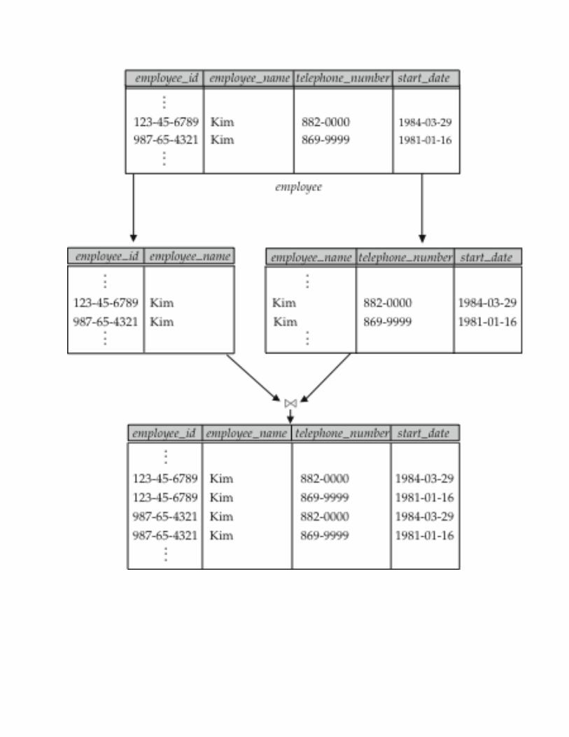
First Normal Form Domain is atomic if its elements are considered to be indivisible units
Examples of non-atomic domains: Set of names, composite attributes Identification numbers like CS101 that can be broken up into parts
A relational schema R is in first normal form if the domains of all attributes of R are atomic
Non-atomic values complicate storage and encourage redundant (repeated) storage of data
Example: Set of accounts stored with each customer, and set of owners stored with each account
Atomicity is actually a property of how the elements of the domain are used.
Example: Strings would normally be considered indivisible
Suppose that students are given roll numbers which are strings of the form CS0012 or EE1127
If the first two characters are extracted to find the department, the domain of roll numbers is not atomic.
Doing so is a bad idea: leads to encoding of information in application program rather than in the database.
Goal — Devise a Theory for
the Following Decide whether a particular relation R is in “good” form.
In the case that a relation R is not in “good” form, decompose it into a set of relations {R1, R2, ..., Rn} such that
each relation is in good form
the decomposition is a lossless-join decomposition
Our theory is based on:
functional dependencies
multivalued dependencies
Functional Dependencies Constraints on the set of legal relations.
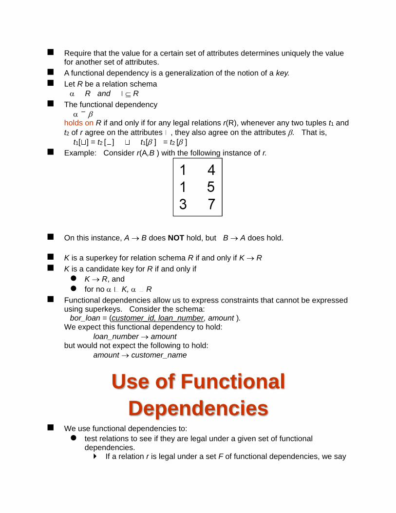
Require that the value for a certain set of attributes determines uniquely the value for another set of attributes.
A functional dependency is a generalization of the notion of a key.
Let R be a relation schema
R and R
The functional dependency
holds on R if and only if for any legal relations r(R), whenever any two tuples t1 and
t2 of r agree on the attributes , they also agree on the attributes . That is,
t1[ ] = t2 [ ] t1[ ] = t2 [ ]
Example: Consider r(A,B ) with the following instance of r.
On this instance, A B does NOT hold, but B A does hold.
K is a superkey for relation schema R if and only if K R
K is a candidate key for R if and only if
K R, and
for no K, R
Functional dependencies allow us to express constraints that cannot be expressed using superkeys. Consider the schema:
bor_loan = (customer_id, loan_number, amount ). We expect this functional dependency to hold:
loan_number amount but would not expect the following to hold:
amount customer_name
Use of Functional
Dependencies We use functional dependencies to:
test relations to see if they are legal under a given set of functional dependencies. If a relation r is legal under a set F of functional dependencies, we say
that r satisfies F.
specify constraints on the set of legal relations We say that F holds on R if all legal relations on R satisfy the set of
functional dependencies F.
Note: A specific instance of a relation schema may satisfy a functional dependency even if the functional dependency does not hold on all legal instances.
For example, a specific instance of loan may, by chance, satisfy
amount customer_name.
A functional dependency is trivial if it is satisfied by all instances of a relation
Example:
customer_name, loan_number customer_name
customer_name customer_name
In general, is trivial if
Closure of a Set of Functional
Dependencies Given a set F of functional dependencies, there are certain other functional
dependencies that are logically implied by F.
For example: If A B and B C, then we can infer that A C
The set of all functional dependencies logically implied by F is the closure of F.
We denote the closure of F by F+.
F+ is a superset of F.
Boyce-Codd Normal Form is trivial (i.e., )
is a superkey for R
Decomposing a Schema into
BCNF Suppose we have a schema R and a non-trivial dependency causes a
violation of BCNF.
We decompose R into:
• (U )
• ( R - ( - ) )
In our example,
= loan_number
= amount and bor_loan is replaced by
(U ) = ( loan_number, amount )
( R - ( - ) ) = ( customer_id, loan_number )
BCNF and Dependency
Preservation Constraints, including functional dependencies, are costly to check in practice
unless they pertain to only one relation
If it is sufficient to test only those dependencies on each individual relation of a decomposition in order to ensure that all functional dependencies hold, then that decomposition is dependency preserving.
Because it is not always possible to achieve both BCNF and dependency preservation, we consider a weaker normal form, known as third normal form.
Third Normal Form A relation schema R is in third normal form (3NF) if for all:
in F+ at least one of the following holds:
is trivial (i.e., )
is a superkey for R
Each attribute A in – is contained in a candidate key for R. (NOTE: each attribute may be in a different candidate key)
If a relation is in BCNF it is in 3NF (since in BCNF one of the first two conditions above must hold).
Third condition is a minimal relaxation of BCNF to ensure dependency preservation (will see why later).
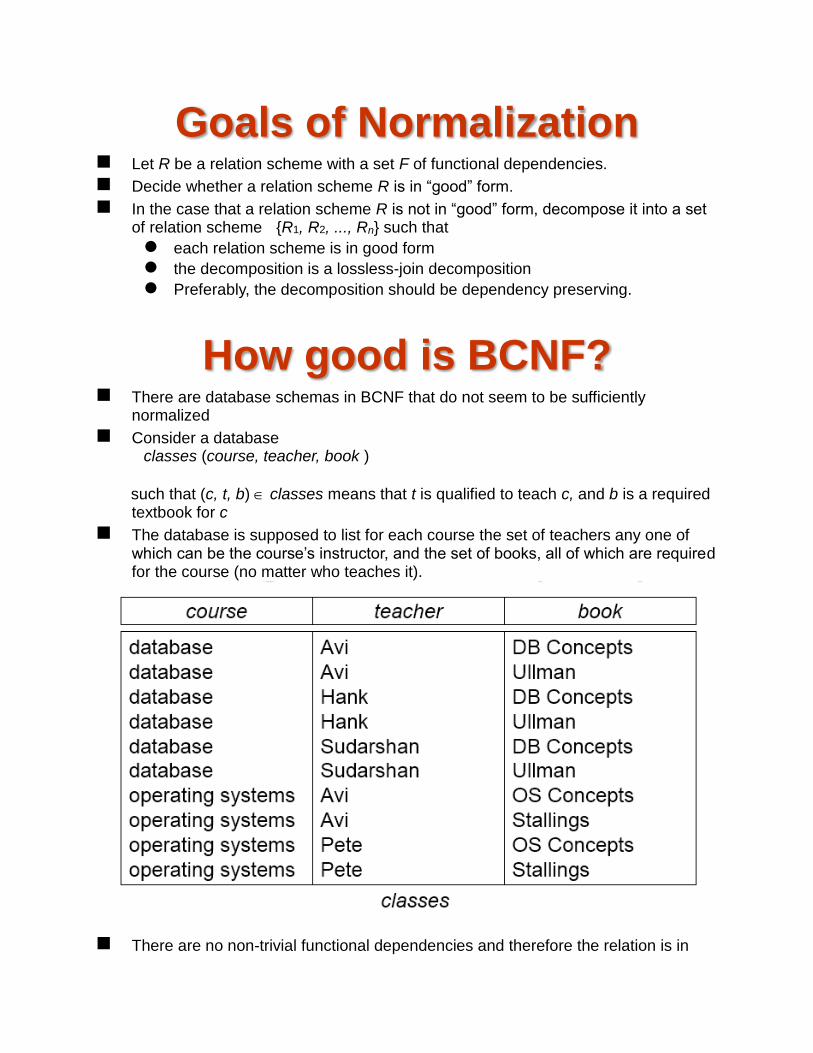
Goals of Normalization Let R be a relation scheme with a set F of functional dependencies.
Decide whether a relation scheme R is in “good” form.
In the case that a relation scheme R is not in “good” form, decompose it into a set of relation scheme {R1, R2, ..., Rn} such that
each relation scheme is in good form
the decomposition is a lossless-join decomposition
Preferably, the decomposition should be dependency preserving.
How good is BCNF? There are database schemas in BCNF that do not seem to be sufficiently
normalized
Consider a database classes (course, teacher, book )
such that (c, t, b) classes means that t is qualified to teach c, and b is a required textbook for c
The database is supposed to list for each course the set of teachers any one of which can be the course’s instructor, and the set of books, all of which are required for the course (no matter who teaches it).
There are no non-trivial functional dependencies and therefore the relation is in
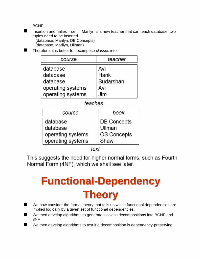
BCNF
Insertion anomalies – i.e., if Marilyn is a new teacher that can teach database, two tuples need to be inserted
(database, Marilyn, DB Concepts) (database, Marilyn, Ullman)
Therefore, it is better to decompose classes into:
Functional-Dependency
Theory We now consider the formal theory that tells us which functional dependencies are
implied logically by a given set of functional dependencies.
We then develop algorithms to generate lossless decompositions into BCNF and 3NF
We then develop algorithms to test if a decomposition is dependency-preserving

Closure of a Set of Functional
Dependencies Given a set F set of functional dependencies, there are certain other functional
dependencies that are logically implied by F.
For example: If A B and B C, then we can infer that A C
The set of all functional dependencies logically implied by F is the closure of F.
We denote the closure of F by F+.
We can find all of F+ by applying Armstrong’s Axioms:
if , then (reflexivity)
if , then (augmentation)
if , and , then (transitivity)
These rules are
sound (generate only functional dependencies that actually hold) and
complete (generate all functional dependencies that hold).
Example R = (A, B, C, G, H, I)
F = { A B
A C
CG H
CG I
B H} some members of F+
A H
by transitivity from A B and B H
AG I
by augmenting A C with G, to get AG CG
and then transitivity with CG I
CG HI
by augmenting CG I to infer CG CGI,
and augmenting of CG H to infer CGI HI, and then transitivity
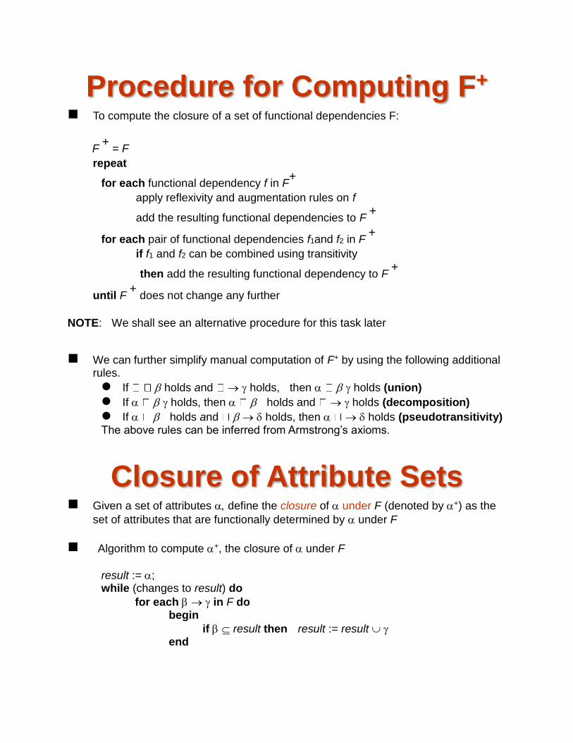
Procedure for Computing F+
To compute the closure of a set of functional dependencies F:
F +
= F
repeat
for each functional dependency f in F+
apply reflexivity and augmentation rules on f
add the resulting functional dependencies to F +
for each pair of functional dependencies f1and f2 in F +
if f1 and f2 can be combined using transitivity
then add the resulting functional dependency to F +
until F +
does not change any further
NOTE: We shall see an alternative procedure for this task later
We can further simplify manual computation of F+ by using the following additional rules.
If holds and holds, then holds (union)
If holds, then holds and holds (decomposition)
If holds and holds, then holds (pseudotransitivity) The above rules can be inferred from Armstrong’s axioms.
Closure of Attribute Sets Given a set of attributes define the closure of under F (denoted by +) as the
set of attributes that are functionally determined by under F
Algorithm to compute +, the closure of under F
result := ; while (changes to result) do
for each in F do begin
if result then result := result end
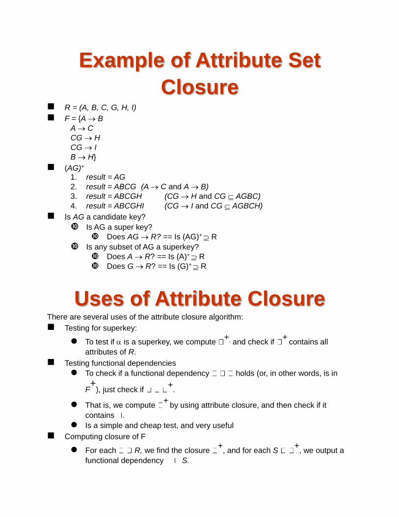
Example of Attribute Set
Closure R = (A, B, C, G, H, I)
F = {A B
A C
CG H
CG I
B H}
(AG)+ 1. result = AG
2. result = ABCG (A C and A B)
3. result = ABCGH (CG H and CG AGBC)
4. result = ABCGHI (CG I and CG AGBCH)
Is AG a candidate key?
Is AG a super key?
Does AG R? == Is (AG)+ R
Is any subset of AG a superkey?
Does A R? == Is (A)+ R
Does G R? == Is (G)+ R
Uses of Attribute Closure There are several uses of the attribute closure algorithm:
Testing for superkey:
To test if is a superkey, we compute +, and check if
+ contains all
attributes of R.
Testing functional dependencies
To check if a functional dependency holds (or, in other words, is in
F+
), just check if +
.
That is, we compute + by using attribute closure, and then check if it
contains .
Is a simple and cheap test, and very useful
Computing closure of F
For each R, we find the closure +
, and for each S +
, we output a
functional dependency S.
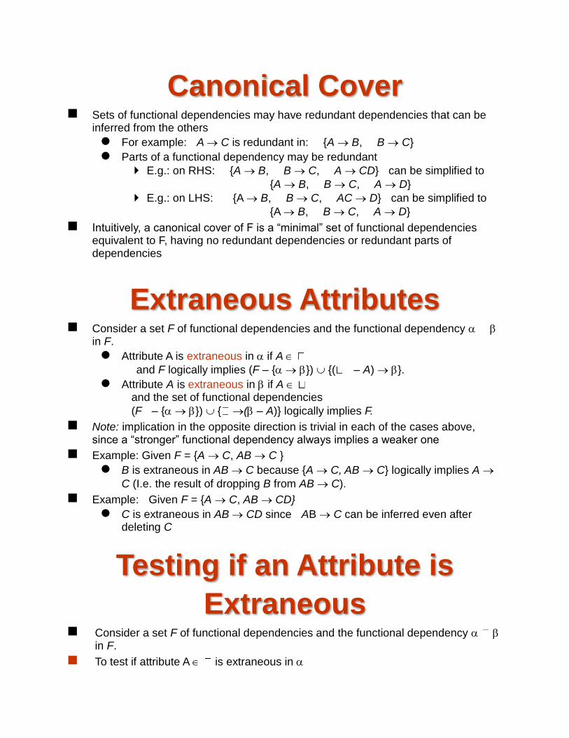
Canonical Cover Sets of functional dependencies may have redundant dependencies that can be
inferred from the others
For example: A C is redundant in: {A B, B C}
Parts of a functional dependency may be redundant
E.g.: on RHS: {A B, B C, A CD} can be simplified to
{A B, B C, A D}
E.g.: on LHS: {A B, B C, AC D} can be simplified to
{A B, B C, A D}
Intuitively, a canonical cover of F is a “minimal” set of functional dependencies equivalent to F, having no redundant dependencies or redundant parts of dependencies
Extraneous Attributes Consider a set F of functional dependencies and the functional dependency
in F.
Attribute A is extraneous in if A
and F logically implies (F – { }) {( – A) }.
Attribute A is extraneous in if A and the set of functional dependencies
(F – { }) { ( – A)} logically implies F.
Note: implication in the opposite direction is trivial in each of the cases above, since a “stronger” functional dependency always implies a weaker one
Example: Given F = {A C, AB C }
B is extraneous in AB C because {A C, AB C} logically implies A
C (I.e. the result of dropping B from AB C).
Example: Given F = {A C, AB CD}
C is extraneous in AB CD since AB C can be inferred even after deleting C
Testing if an Attribute is
Extraneous Consider a set F of functional dependencies and the functional dependency
in F.
To test if attribute A is extraneous in

compute ({} – A)+
using the dependencies in F
check that ({} – A)+
contains ; if it does, A is extraneous in
To test if attribute A is extraneous in
compute +
using only the dependencies in
F’ = (F – { }) { ( – A)},
check that +
contains A; if it does, A is extraneous in
Canonical Cover A canonical cover for F is a set of dependencies Fc such that
F logically implies all dependencies in Fc, and
Fc logically implies all dependencies in F, and
No functional dependency in Fc contains an extraneous attribute, and
Each left side of functional dependency in Fc is unique.
To compute a canonical cover for F: repeat Use the union rule to replace any dependencies in F
1 1 and 1 2 with 1 1 2
Find a functional dependency with an
extraneous attribute either in or in
If an extraneous attribute is found, delete it from until F does not change
Note: Union rule may become applicable after some extraneous attributes have been deleted, so it has to be re-applied
Computing a Canonical Cover R = (A, B, C)
F = {A BC
B C
A B
AB C}
Combine A BC and A B into A BC
Set is now {A BC, B C, AB C}
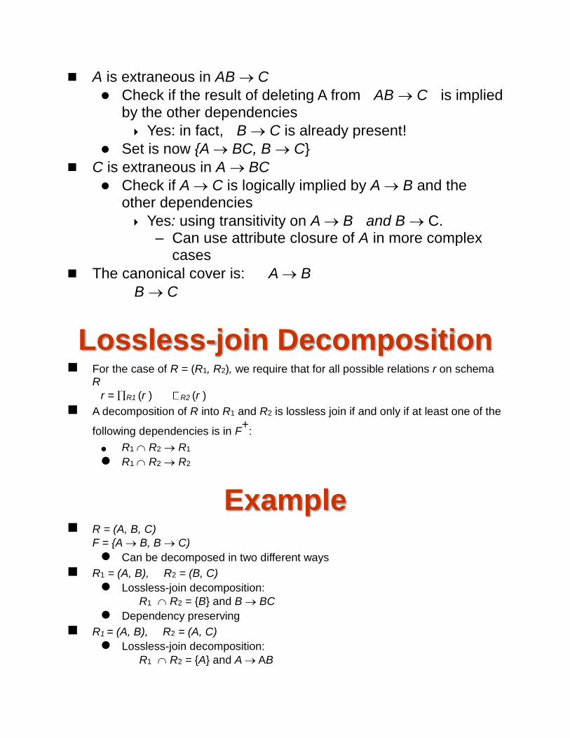
A is extraneous in AB C
Check if the result of deleting A from AB C is implied by the other dependencies
Yes: in fact, B C is already present!
Set is now {A BC, B C}
C is extraneous in A BC
Check if A C is logically implied by A B and the other dependencies
Yes: using transitivity on A B and B C. – Can use attribute closure of A in more complex
cases
The canonical cover is: A B
B C
Lossless-join Decomposition For the case of R = (R1, R2), we require that for all possible relations r on schema
R
r = R1 (r ) R2 (r )
A decomposition of R into R1 and R2 is lossless join if and only if at least one of the
following dependencies is in F+
:
R1 R2 R1
R1 R2 R2
Example R = (A, B, C)
F = {A B, B C)
Can be decomposed in two different ways
R1 = (A, B), R2 = (B, C)
Lossless-join decomposition:
R1 R2 = {B} and B BC
Dependency preserving
R1 = (A, B), R2 = (A, C)
Lossless-join decomposition:
R1 R2 = {A} and A AB
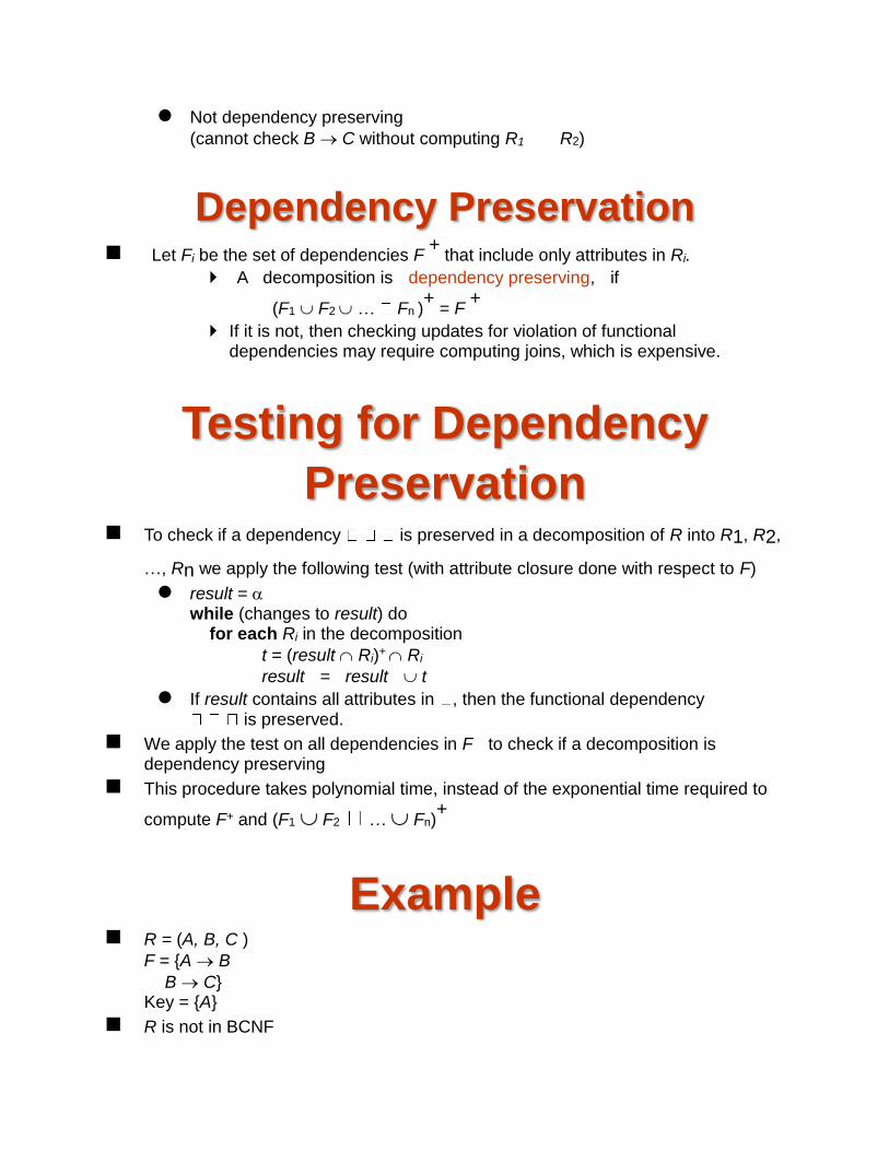
Not dependency preserving
(cannot check B C without computing R1 R2)
Dependency Preservation Let Fi be the set of dependencies F
+ that include only attributes in Ri.
A decomposition is dependency preserving, if
(F1 F2 … Fn )+
= F +
If it is not, then checking updates for violation of functional dependencies may require computing joins, which is expensive.
Testing for Dependency
Preservation To check if a dependency is preserved in a decomposition of R into R1, R2,
…, Rn we apply the following test (with attribute closure done with respect to F)
result = while (changes to result) do for each Ri in the decomposition
t = (result Ri)+ Ri
result = result t
If result contains all attributes in , then the functional dependency is preserved.
We apply the test on all dependencies in F to check if a decomposition is dependency preserving
This procedure takes polynomial time, instead of the exponential time required to
compute F+ and (F1 F2 … Fn)+
Example R = (A, B, C )
F = {A B
B C} Key = {A}
R is not in BCNF

Decomposition R1 = (A, B), R2 = (B, C)
R1 and R2 in BCNF
Lossless-join decomposition
Dependency preserving
Comparison of BCNF and 3NF It is always possible to decompose a relation into a set of relations that are in
3NF such that:
the decomposition is lossless
the dependencies are preserved
It is always possible to decompose a relation into a set of relations that are in BCNF such that:
the decomposition is lossless
it may not be possible to preserve dependencies.
Design Goals Goal for a relational database design is:
BCNF.
Lossless join.
Dependency preservation.
If we cannot achieve this, we accept one of
Lack of dependency preservation
Redundancy due to use of 3NF
Interestingly, SQL does not provide a direct way of specifying functional dependencies other than superkeys.
Can specify FDs using assertions, but they are expensive to test
Even if we had a dependency preserving decomposition, using SQL we would not be able to efficiently test a functional dependency whose left hand side is not a key.
Overall Database Design
Process We have assumed schema R is given
R could have been generated when converting E-R diagram to a set of
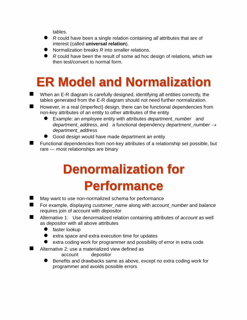
tables.
R could have been a single relation containing all attributes that are of interest (called universal relation).
Normalization breaks R into smaller relations.
R could have been the result of some ad hoc design of relations, which we then test/convert to normal form.
ER Model and Normalization When an E-R diagram is carefully designed, identifying all entities correctly, the
tables generated from the E-R diagram should not need further normalization.
However, in a real (imperfect) design, there can be functional dependencies from non-key attributes of an entity to other attributes of the entity
Example: an employee entity with attributes department_number and
department_address, and a functional dependency department_number department_address
Good design would have made department an entity
Functional dependencies from non-key attributes of a relationship set possible, but rare --- most relationships are binary
Denormalization for
Performance May want to use non-normalized schema for performance
For example, displaying customer_name along with account_number and balance requires join of account with depositor
Alternative 1: Use denormalized relation containing attributes of account as well as depositor with all above attributes
faster lookup
extra space and extra execution time for updates
extra coding work for programmer and possibility of error in extra code
Alternative 2: use a materialized view defined as account depositor
Benefits and drawbacks same as above, except no extra coding work for programmer and avoids possible errors
Other Design Issues Some aspects of database design are not caught by normalization
Examples of bad database design, to be avoided: Instead of earnings (company_id, year, amount ), use
earnings_2004, earnings_2005, earnings_2006, etc., all on the schema (company_id, earnings). Above are in BCNF, but make querying across years difficult and needs
new table each year
company_year(company_id, earnings_2004, earnings_2005, earnings_2006) Also in BCNF, but also makes querying across years difficult and
requires new attribute each year. Is an example of a crosstab, where values for one attribute become
column names Used in spreadsheets, and in data analysis tools
Modeling Temporal Data Temporal data have an association time interval during which the data are valid.
A snapshot is the value of the data at a particular point in time
Several proposals to extend ER model by adding valid time to
attributes, e.g. address of a customer at different points in time
entities, e.g. time duration when an account exists
relationships, e.g. time during which a customer owned an account
But no accepted standard
Adding a temporal component results in functional dependencies like
customer_id customer_street, customer_city not to hold, because the address varies over time
A temporal functional dependency X Y holds on schema R if the functional dependency X Y holds on all snapshots for all legal instances r (R )
In practice, database designers may add start and end time attributes to relations
E.g. course(course_id, course_title) course(course_id, course_title, start, end) Constraint: no two tuples can have overlapping valid times
– Hard to enforce efficiently
Foreign key references may be to current version of data, or to data at a point in time
E.g. student transcript should refer to course information at the time the course was taken

2014
11/16/2014

Triggers A trigger is a statement that is executed automatically by the system as a side
effect of a modification to the database.
To design a trigger mechanism, we must:
Specify the conditions under which the trigger is to be executed.
Specify the actions to be taken when the trigger executes.
Triggers introduced to SQL standard in SQL:1999, but supported even earlier using non-standard syntax by most databases.
Trigger Example Suppose that instead of allowing negative account balances, the bank deals with
overdrafts by
setting the account balance to zero
creating a loan in the amount of the overdraft
giving this loan a loan number identical to the account number of the overdrawn account
The condition for executing the trigger is an update to the account relation that results in a negative balance value.
Trigger Example in SQL:1999 create trigger overdraft-trigger after update on account
referencing new row as nrow for each row when nrow.balance < 0 begin atomic insert into borrower (select customer-name, account-number from depositor where nrow.account-number = depositor.account-number); insert into loan values (n.row.account-number, nrow.branch-name, – nrow.balance); update account set balance = 0 where account.account-number = nrow.account-number end
Triggering Events and Actions
in SQL Triggering event can be insert, delete or update
Triggers on update can be restricted to specific attributes
E.g. create trigger overdraft-trigger after update of balance on account
Values of attributes before and after an update can be referenced
referencing old row as : for deletes and updates
referencing new row as : for inserts and updates
Triggers can be activated before an event, which can serve as extra constraints. E.g. convert blanks to null.
create trigger setnull-trigger before update on r referencing new row as nrow for each row when nrow.phone-number = ‘ ‘ set nrow.phone-number = null
Statement Level Triggers Instead of executing a separate action for each affected row, a single action can be
executed for all rows affected by a transaction
Use for each statement instead of for each row
Use referencing old table or referencing new table to refer to temporary tables (called transition tables) containing the affected rows
Can be more efficient when dealing with SQL statements that update a large number of rows
External World Actions We sometimes require external world actions to be triggered
on a database update E.g. re-ordering an item whose quantity in a warehouse
has become small, or turning on an alarm light, Triggers cannot be used to directly implement external-world
actions, BUT Triggers can be used to record actions-to-be-taken in a
separate table Have an external process that repeatedly scans the table,
carries out external-world actions and deletes action from table
E.g. Suppose a warehouse has the following tables inventory (item, level ): How much of each item is in the
warehouse minlevel (item, level ) : What is the minimum desired
level of each item reorder (item, amount ): What quantity should we re-
order at a time orders (item, amount ) : Orders to be placed (read by
external process) create trigger reorder-trigger after update of amount on inventory referencing old row as orow, new row as nrow for each row when nrow.level < = (select level from minlevel where minlevel.item = orow.item) and orow.level > (select level from minlevel where minlevel.item = orow.item) begin insert into orders (select item, amount from reorder where reorder.item = orow.item) end
Triggers in MS-SQLServer
Syntax create trigger overdraft-trigger on account
for update as if inserted.balance < 0 begin insert into borrower
(select customer-name,account-number from depositor, inserted where inserted.account-number = depositor.account-number) insert into loan values (inserted.account-number, inserted.branch-name, – inserted.balance) update account set balance = 0 from account, inserted where account.account-number = inserted.account-number end
When Not To Use Triggers Triggers were used earlier for tasks such as
maintaining summary data (e.g. total salary of each department)
Replicating databases by recording changes to special relations (called change or delta relations) and having a separate process that applies the changes over to a replica
There are better ways of doing these now:
Databases today provide built in materialized view facilities to maintain summary data
Databases provide built-in support for replication
Encapsulation facilities can be used instead of triggers in many cases
Define methods to update fields
Carry out actions as part of the update methods instead of through a trigger
Authorization in SQL Forms of authorization on parts of the database:
Read authorization - allows reading, but not modification of data.
Insert authorization - allows insertion of new data, but not modification of existing data.
Update authorization - allows modification, but not deletion of data.
Delete authorization - allows deletion of data Forms of authorization to modify the database schema:
Index authorization - allows creation and deletion of indices.
Resources authorization - allows creation of new relations.
Alteration authorization - allows addition or deletion of attributes in a relation.
Drop authorization - allows deletion of relations.
Authorization and Views Users can be given authorization on views, without being given any authorization
on the relations used in the view definition
Ability of views to hide data serves both to simplify usage of the system and to enhance security by allowing users access only to data they need for their job
A combination or relational-level security and view-level security can be used to limit a user’s access to precisely the data that user needs.
View Example Suppose a bank clerk needs to know the names of the customers of each branch,
but is not authorized to see specific loan information.
Approach: Deny direct access to the loan relation, but grant access to the view cust-loan, which consists only of the names of customers and the branches at which they have a loan.
The cust-loan view is defined in SQL as follows: create view cust-loan as
select branchname, customer-name from borrower, loan where borrower.loan-number = loan.loan-number
The clerk is authorized to see the result of the query: select *
from cust-loan
When the query processor translates the result into a query on the actual relations in the database, we obtain a query on borrower and loan.
Authorization must be checked on the clerk’s query before query processing replaces a view by the definition of the view.
Authorization on Views Creation of view does not require resources authorization since no real relation is
being created
The creator of a view gets only those privileges that provide no additional
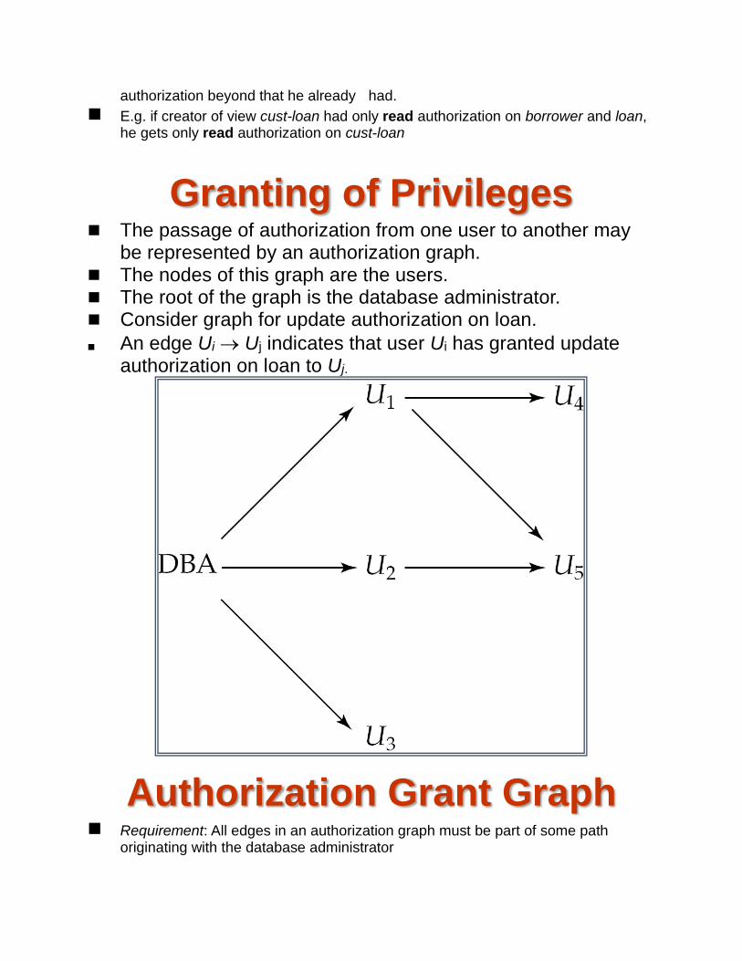
authorization beyond that he already had.
E.g. if creator of view cust-loan had only read authorization on borrower and loan, he gets only read authorization on cust-loan
Granting of Privileges The passage of authorization from one user to another may
be represented by an authorization graph. The nodes of this graph are the users. The root of the graph is the database administrator. Consider graph for update authorization on loan.
An edge Ui Uj indicates that user Ui has granted update authorization on loan to Uj.
Authorization Grant Graph Requirement: All edges in an authorization graph must be part of some path
originating with the database administrator
If DBA revokes grant from U1:
Grant must be revoked from U4 since U1 no longer has authorization
Grant must not be revoked from U5 since U5 has another authorization path from DBA through U2
Must prevent cycles of grants with no path from the root:
DBA grants authorization to U7
U7 grants authorization to U8
U8 grants authorization to U7
DBA revokes authorization from U7
Must revoke grant U7 to U8 and from U8 to U7 since there is no path from DBA to U7 or to U8 anymore.
Security Specification in SQL The grant statement is used to confer authorization grant <privilege list> on <relation name or view name> to <user list>
<user list> is:
a user-id
public, which allows all valid users the privilege granted
A role (more on this later)
Granting a privilege on a view does not imply granting any privileges on the underlying relations.
The grantor of the privilege must already hold the privilege on the specified item (or be the database administrator).
Privileges in SQL select: allows read access to relation,or the ability to query using the view
Example: grant users U1, U2, and U3 select authorization on the branch relation:
grant select on branch to U1, U2, U3
insert: the ability to insert tuples
update: the ability to update using the SQL update statement
delete: the ability to delete tuples.
references: ability to declare foreign keys when creating relations.
usage: In SQL-92; authorizes a user to use a specified domain
all privileges: used as a short form for all the allowable privileges
Privilege To Grant Privileges with grant option: allows a user who is granted a privilege to pass the privilege on
to other users.
Example: grant select on branch to U1 with grant option
gives U1 the select privileges on branch and allows U1 to grant this privilege to others
Roles Roles permit common privileges for a class of users can be specified just once by
creating a corresponding “role”
Privileges can be granted to or revoked from roles, just like user
Roles can be assigned to users, and even to other roles
SQL:1999 supports roles create role teller
create role manager
grant select on branch to teller grant update (balance) on account to teller grant all privileges on account to manager grant teller to manager grant teller to alice, bob grant manager to avi
Revoking Authorization in
SQL The revoke statement is used to revoke authorization.
revoke<privilege list> on <relation name or view name> from <user list> [restrict|cascade]
Example: revoke select on branch from U1, U2, U3 cascade
Revocation of a privilege from a user may cause other users also to lose that
privilege; referred to as cascading of the revoke.
We can prevent cascading by specifying restrict: revoke select on branch from U1, U2, U3 restrict
With restrict, the revoke command fails if cascading revokes are required.
<privilege-list> may be all to revoke all privileges the revokee may hold.
If <revokee-list> includes public all users lose the privilege except those granted it explicitly.
If the same privilege was granted twice to the same user by different grantees, the user may retain the privilege after the revocation.
All privileges that depend on the privilege being revoked are also revoked.
Limitations of SQL
Authorization SQL does not support authorization at a tuple level
E.g. we cannot restrict students to see only (the tuples storing) their own grades
With the growth in Web access to databases, database accesses come primarily from application servers. End users don't have database user ids, they are all
mapped to the same database user id All end-users of an application (such as a web application)
may be mapped to a single database user The task of authorization in above cases falls on the
application program, with no support from SQL Benefit: fine grained authorizations, such as to individual
tuples, can be implemented by the application. Drawback: Authorization must be done in application
code, and may be dispersed all over an application Checking for absence of authorization loopholes
becomes very difficult since it requires reading large amounts of application code
Audit Trails An audit trail is a log of all changes (inserts/deletes/updates) to the database along
with information such as which user performed the change, and when the change was performed.
Used to track erroneous/fraudulent updates.
Can be implemented using triggers, but many database systems provide direct support.
Application Security Data may be encrypted when database authorization provisions do not offer
sufficient protection.
Properties of good encryption technique:
Relatively simple for authorized users to encrypt and decrypt data.
Encryption scheme depends not on the secrecy of the algorithm but on the secrecy of a parameter of the algorithm called the encryption key.
Extremely difficult for an intruder to determine the encryption key.
Encryption (Cont.) Data Encryption Standard (DES) substitutes characters and
rearranges their order on the basis of an encryption key which is provided to authorized users via a secure mechanism. Scheme is no more secure than the key transmission mechanism since the key has to be shared.
Advanced Encryption Standard (AES) is a new standard replacing DES, and is based on the Rijndael algorithm, but is also dependent on shared secret keys
Public-key encryption is based on each user having two keys: public key – publicly published key used to encrypt data,
but cannot be used to decrypt data private key -- key known only to individual user, and
used to decrypt data. Need not be transmitted to the site doing encryption.
Encryption scheme is such that it is impossible or extremely hard to decrypt data given only the public key.
The RSA public-key encryption scheme is based on the hardness of factoring a very large number (100's of digits) into its prime components.
Authentication Password based authentication is widely used, but is
susceptible to sniffing on a network Challenge-response systems avoid transmission of
passwords DB sends a (randomly generated) challenge string to
user User encrypts string and returns result. DB verifies identity by decrypting result Can use public-key encryption system by DB sending a
message encrypted using user’s public key, and user decrypting and sending the message back
Digital signatures are used to verify authenticity of data E.g. use private key (in reverse) to encrypt data, and
anyone can verify authenticity by using public key (in reverse) to decrypt data. Only holder of private key could have created the encrypted data.
Digital signatures also help ensure nonrepudiation: sender cannot later claim to have not created the data
Digital Certificates Digital certificates are used to verify authenticity of public
keys. Problem: when you communicate with a web site, how do you
know if you are talking with the genuine web site or an

imposter? Solution: use the public key of the web site Problem: how to verify if the public key itself is genuine?
Solution: Every client (e.g. browser) has public keys of a few root-
level certification authorities A site can get its name/URL and public key signed by a
certification authority: signed document is called a certificate
Client can use public key of certification authority to verify certificate
Multiple levels of certification authorities can exist. Each certification authority presents its own public-key certificate signed by a
higher level authority, and Uses its private key to sign the certificate of other
web sites/authorities

2014
11/16/2014
Object-Based Databases Complex Data Types and Object Orientation
Structured Data Types and Inheritance in SQL
Table Inheritance
Array and Multiset Types in SQL
Object Identity and Reference Types in SQL
Implementing O-R Features
Comparison of Object-Oriented and Object-Relational Databases
Object-Relational Data Models Extend the relational data model by including object orientation and constructs to
deal with added data types.
Allow attributes of tuples to have complex types, including non-atomic values such as nested relations.
Preserve relational foundations, in particular the declarative access to data, while extending modeling power.
Upward compatibility with existing relational languages.
Complex Data Types Motivation:
Permit non-atomic domains (atomic indivisible)
Example of non-atomic domain: set of integers,or set of tuples
Allows more intuitive modeling for applications with complex data
Intuitive definition:
allow relations whenever we allow atomic (scalar) values — relations within relations
Retains mathematical foundation of relational model
Violates first normal form.
Example of a Nested Relation Example: library information system
Each book has
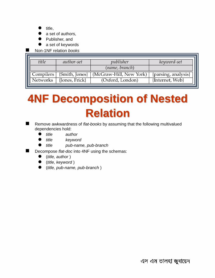
title,
a set of authors,
Publisher, and
a set of keywords
Non-1NF relation books
4NF Decomposition of Nested
Relation Remove awkwardness of flat-books by assuming that the following multivalued
dependencies hold:
title author
title keyword
title pub-name, pub-branch
Decompose flat-doc into 4NF using the schemas:
(title, author )
(title, keyword )
(title, pub-name, pub-branch )

4NF Decomposition of flat–
books
Problems with 4NF Schema 4NF design requires users to include joins in their queries.
1NF relational view flat-books defined by join of 4NF relations:
eliminates the need for users to perform joins,
but loses the one-to-one correspondence between tuples and documents.
And has a large amount of redundancy
Nested relations representation is much more natural here.
Complex Types Extensions to SQL to support complex types include:
Collection and large object types
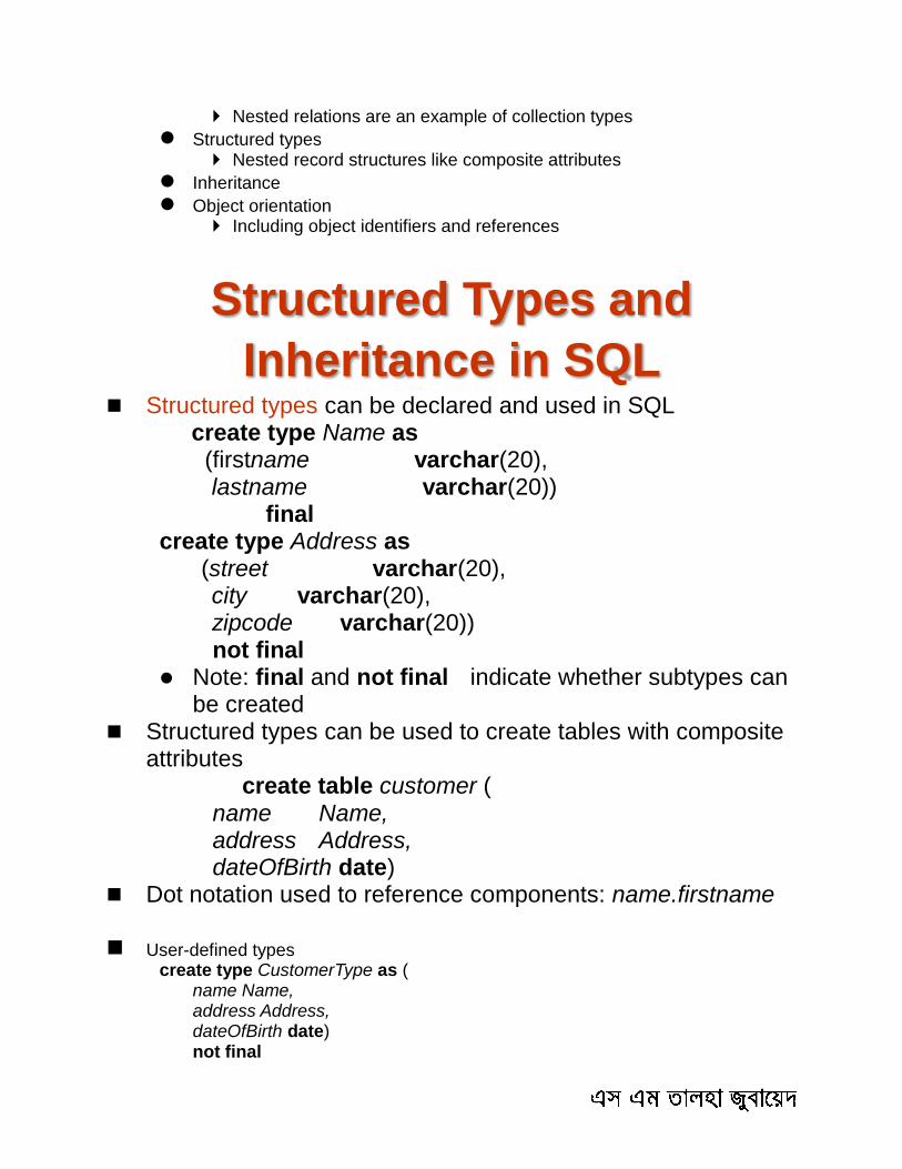
Nested relations are an example of collection types
Structured types Nested record structures like composite attributes
Inheritance
Object orientation Including object identifiers and references
Structured Types and
Inheritance in SQL Structured types can be declared and used in SQL create type Name as
(firstname varchar(20), lastname varchar(20)) final
create type Address as (street varchar(20), city varchar(20), zipcode varchar(20))
not final Note: final and not final indicate whether subtypes can
be created Structured types can be used to create tables with composite
attributes create table customer ( name Name, address Address, dateOfBirth date) Dot notation used to reference components: name.firstname
User-defined types
create type CustomerType as ( name Name, address Address, dateOfBirth date) not final
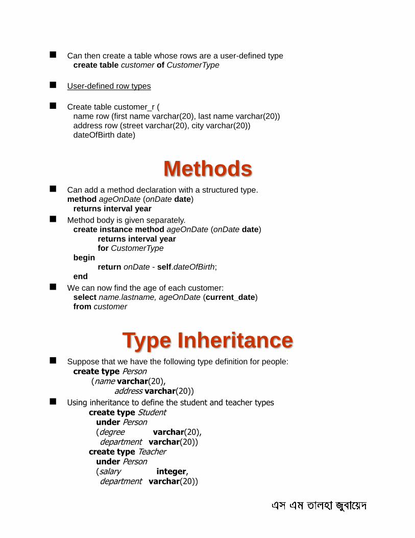
Can then create a table whose rows are a user-defined type create table customer of CustomerType
User-defined row types
Create table customer_r ( name row (first name varchar(20), last name varchar(20)) address row (street varchar(20), city varchar(20)) dateOfBirth date)
Methods Can add a method declaration with a structured type. method ageOnDate (onDate date) returns interval year
Method body is given separately. create instance method ageOnDate (onDate date) returns interval year for CustomerType begin return onDate - self.dateOfBirth; end
We can now find the age of each customer: select name.lastname, ageOnDate (current_date) from customer
Type Inheritance Suppose that we have the following type definition for people:
create type Person (name varchar(20), address varchar(20))
Using inheritance to define the student and teacher types create type Student under Person (degree varchar(20), department varchar(20)) create type Teacher under Person (salary integer, department varchar(20))
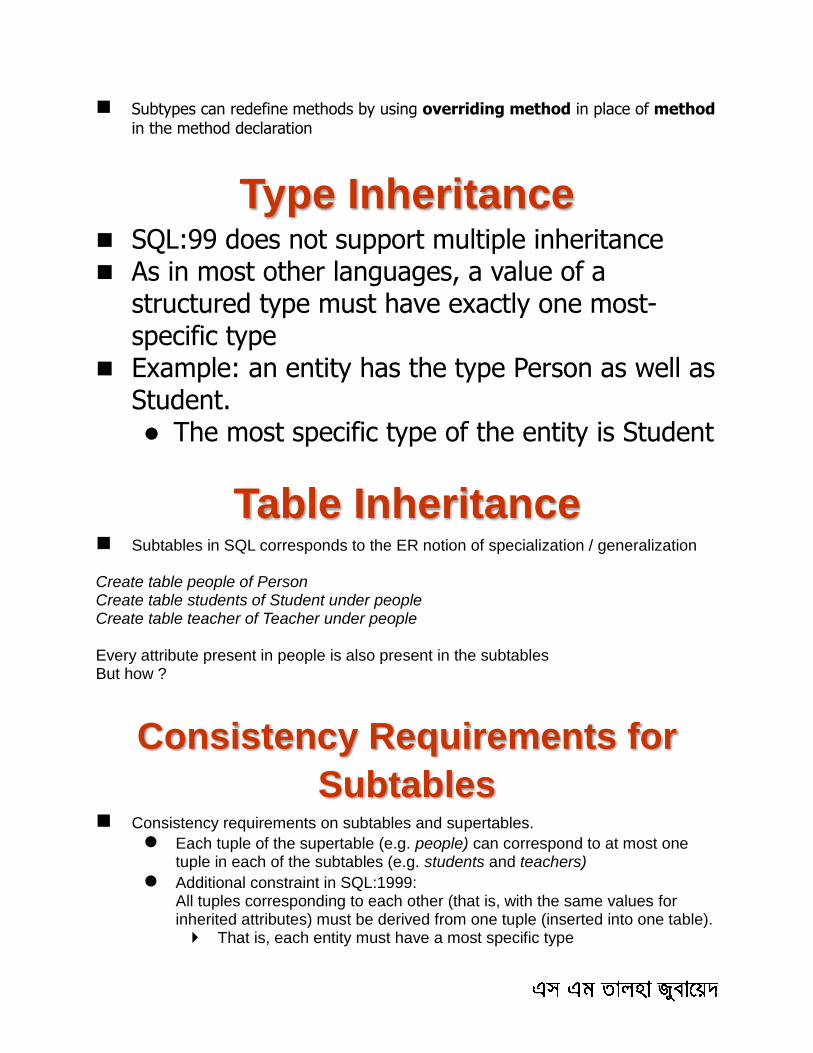
Subtypes can redefine methods by using overriding method in place of method in the method declaration
Type Inheritance SQL:99 does not support multiple inheritance As in most other languages, a value of a
structured type must have exactly one most-specific type
Example: an entity has the type Person as well as Student. The most specific type of the entity is Student
Table Inheritance Subtables in SQL corresponds to the ER notion of specialization / generalization Create table people of Person Create table students of Student under people Create table teacher of Teacher under people Every attribute present in people is also present in the subtables But how ?
Consistency Requirements for
Subtables Consistency requirements on subtables and supertables.
Each tuple of the supertable (e.g. people) can correspond to at most one tuple in each of the subtables (e.g. students and teachers)
Additional constraint in SQL:1999: All tuples corresponding to each other (that is, with the same values for
inherited attributes) must be derived from one tuple (inserted into one table). That is, each entity must have a most specific type
We cannot have a tuple in people corresponding to a tuple each in students and teachers
Array and Multiset Types in
SQL Example of array and multiset declaration: create type Publisher as
(name varchar(20), branch varchar(20)) create type Book as (title varchar(20), author-array varchar(20) array [10], pub-date date, publisher Publisher, keyword-set varchar(20) multiset )
create table books of Book Similar to the nested relation books, but with array of authors
instead of set
Creation of Collection Values Array construction array [‘Silberschatz’,`Korth’,`Sudarshan’]
Multisets
multisetset [‘computer’, ‘database’, ‘SQL’]
To create a tuple of the type defined by the books relation: (‘Compilers’, array[`Smith’,`Jones’], Publisher (`McGraw-Hill’,`New York’), multiset [`parsing’,`analysis’ ])
To insert the preceding tuple into the relation books insert into books
values (‘Compilers’, array[`Smith’,`Jones’], Publisher (`McGraw-Hill’,`New York’),
multiset [`parsing’,`analysis’ ])
Querying Collection-Valued
Attributes To find all books that have the word “database” as a keyword, select title
from books where ‘database’ in (unnest(keyword-set ))
We can access individual elements of an array by using indices
E.g.: If we know that a particular book has three authors, we could write: select author-array[1], author-array[2], author-array[3]
from books where title = `Database System Concepts’
To get a relation containing pairs of the form “title, author-name” for each book and each author of the book
select B.title, A.author from books as B, unnest (B.author-array) as A (author )
To retain ordering information we add a with ordinality clause select B.title, A.author, A.position from books as B, unnest (B.author-array) with ordinality as A (author, position )
Unnesting The transformation of a nested relation into a
form with fewer (or no) relation-valued attributes us called unnesting.
E.g. select title, A as author, publisher.name as
pub_name, publisher.branch as pub_branch,
K.keyword from books as B, unnest(B.author_array ) as
A (author ), unnest (B.keyword_set ) as K (keyword )
Object-Identity and Reference
Types Define a type Department with a field name and a field head which is a reference
to the type Person, with table people as scope: create type Department (
name varchar (20), head ref (Person) scope people)
We can then create a table departments as follows create table departments of Department
We can omit the declaration scope people from the type declaration and instead make an addition to the create table statement: create table departments of Department (head with options scope people)
Initializing Reference-Typed
Values Create table people of Person ref is person_id system generated
To create a tuple with a reference value, we can first create the tuple with a null reference and then set the reference separately:
insert into departments values (`CS’, null) update departments set head = (select p.person_id from people as p where name = `John’) where name = `CS’
User Generated Identifiers The type of the object-identifier must be specified as part of the type definition of
the referenced table, and
The table definition must specify that the reference is user generated create type Person
(name varchar(20) address varchar(20)) ref using varchar(20) create table people of Person ref is person_id user generated
When creating a tuple, we must provide a unique value for the identifier:
insert into people (person_id, name, address ) values (‘02184567’, ‘John’, `23 Coyote Run’)
We can then use the identifier value when inserting a tuple into departments
Avoids need for a separate query to retrieve the identifier: insert into departments
values(`CS’, `02184567’)
Can use an existing primary key value as the identifier: create type Person
(name varchar (20) primary key, address varchar(20)) ref from (name) create table people of Person ref is person_id derived
When inserting a tuple for departments, we can then use insert into departments
values(`CS’,`John’)
Path Expressions Find the names and addresses of the heads of all departments:
select head –>name, head –>address from departments
An expression such as “head–>name” is called a path expression
Path expressions help avoid explicit joins
If department head were not a reference, a join of departments with people would be required to get at the address
Makes expressing the query much easier for the user
Implementing O-R Features Multi-valued attributes in ER model correspont to multi-set valued attributes
Composite attributes correspond to structured types
ISA hierarchy correspond to table inheritance
Implementing O-R Features Similar to how E-R features are mapped onto relation schemas
Subtable implementation
Each table stores primary key and those attributes defined in that table or,
Each table stores both locally defined and inherited attributes
Persistent Programming
Languages Languages extended with constructs to handle persistent data
Programmer can manipulate persistent data directly
no need to fetch it into memory and store it back to disk (unlike embedded SQL)
Persistent objects:
by class - explicit declaration of persistence
by creation - special syntax to create persistent objects
by marking - make objects persistent after creation
by reachability - object is persistent if it is declared explicitly to be so or is reachable from a persistent object
Object Identity and Pointers Degrees of permanence of object identity
Intraprocedure: only during execution of a single procedure
Intraprogram: only during execution of a single program or query
Interprogram: across program executions, but not if data-storage format on disk changes
Persistent: interprogram, plus persistent across data reorganizations
Persistent versions of C++ and Java have been implemented
C++ ODMG C++ ObjectStore
Java Java Database Objects (JDO)
Comparison of O-O and O-R
Databases
Relational systems
simple data types, powerful query languages, high protection.
Persistent-programming-language-based OODBs
complex data types, integration with programming language, high performance.
Object-relational systems
complex data types, powerful query languages, high protection.
Note: Many real systems blur these boundaries
E.g. persistent programming language built as a wrapper on a relational database offers first two benefits, but may have poor performance.

2014
11/16/2014
Storage and File Structure Overview of Physical Storage Media
Magnetic Disks
RAID
Tertiary Storage
Storage Access
File Organization
Organization of Records in Files
Data-Dictionary Storage
Storage Structures for Object-Oriented Databases
Classification of Physical
Storage Media Speed with which data can be accessed
Cost per unit of data
Reliability
data loss on power failure or system crash
physical failure of the storage device
Can differentiate storage into:
volatile storage: loses contents when power is switched off
non-volatile storage: Contents persist even when power is switched off. Includes secondary and tertiary storage, as well as batter- backed
up main-memory.
Physical Storage Media Cache – fastest and most costly form of storage; volatile; managed by the
computer system hardware.
Main memory:
fast access (10s to 100s of nanoseconds; 1 nanosecond = 10–9
seconds)
generally too small (or too expensive) to store the entire database capacities of up to a few Gigabytes widely used currently Capacities have gone up and per-byte costs have decreased steadily
and rapidly (roughly factor of 2 every 2 to 3 years)
Volatile — contents of main memory are usually lost if a power failure or system crash occurs.
Flash memory
Data survives power failure
Data can be written at a location only once, but location can be erased and written to again Can support only a limited number (10K – 1M) of write/erase cycles. Erasing of memory has to be done to an entire bank of memory
Reads are roughly as fast as main memory
But writes are slow (few microseconds), erase is slower
Cost per unit of storage roughly similar to main memory
Widely used in embedded devices such as digital cameras
Is a type of EEPROM (Electrically Erasable Programmable Read-Only Memory)
Magnetic-disk
Data is stored on spinning disk, and read/written magnetically
Primary medium for the long-term storage of data; typically stores entire database.
Data must be moved from disk to main memory for access, and written back for storage Much slower access than main memory (more on this
later) direct-access – possible to read data on disk in any
order, unlike magnetic tape Capacities range up to roughly 400 GB currently
Much larger capacity and cost/byte than main memory/flash memory
Growing constantly and rapidly with technology improvements (factor of 2 to 3 every 2 years)
Survives power failures and system crashes disk failure can destroy data, but is rare
Optical storage
non-volatile, data is read optically from a spinning disk using a laser
CD-ROM (640 MB) and DVD (4.7 to 17 GB) most popular forms
Write-one, read-many (WORM) optical disks used for archival storage (CD-R, DVD-R, DVD+R)
Multiple write versions also available (CD-RW, DVD-RW, DVD+RW, and DVD-RAM)
Reads and writes are slower than with magnetic disk
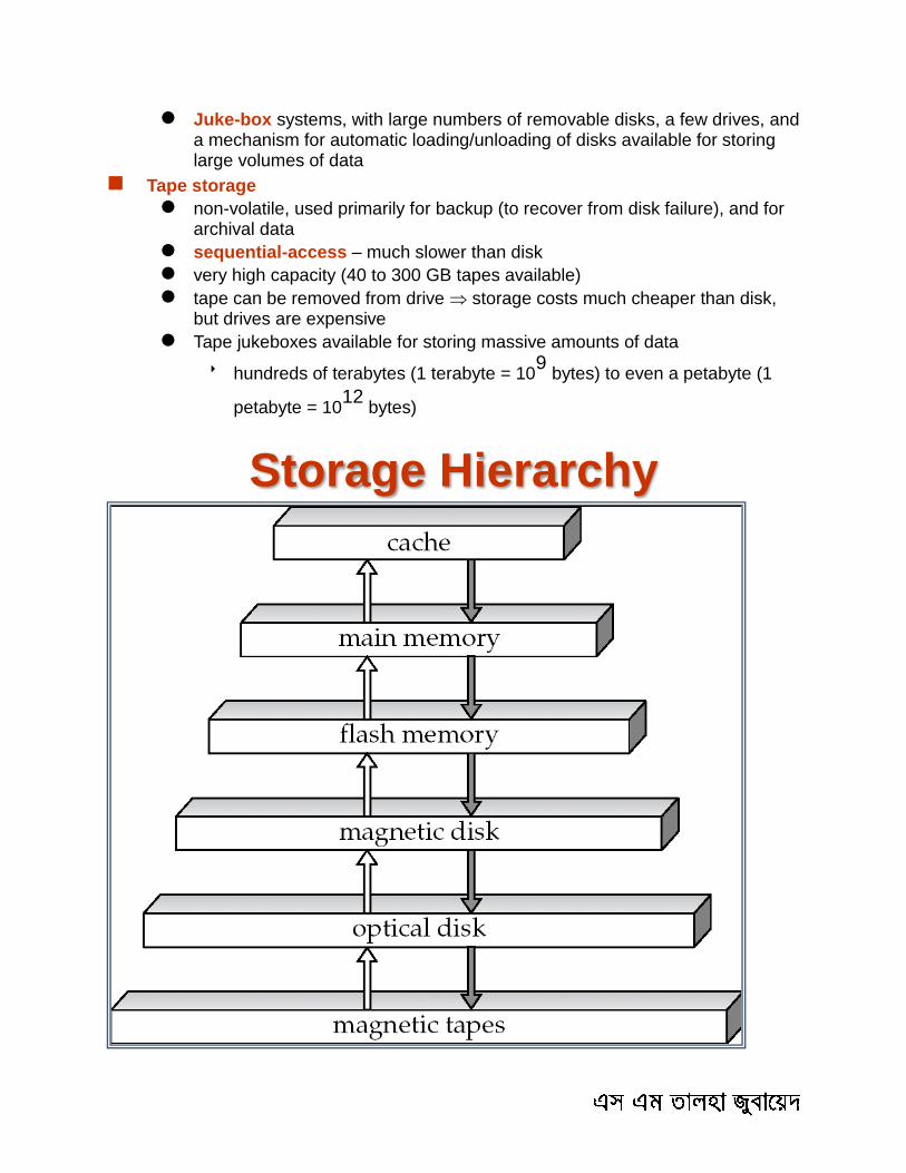
Juke-box systems, with large numbers of removable disks, a few drives, and a mechanism for automatic loading/unloading of disks available for storing large volumes of data
Tape storage
non-volatile, used primarily for backup (to recover from disk failure), and for archival data
sequential-access – much slower than disk
very high capacity (40 to 300 GB tapes available)
tape can be removed from drive storage costs much cheaper than disk, but drives are expensive
Tape jukeboxes available for storing massive amounts of data
hundreds of terabytes (1 terabyte = 109
bytes) to even a petabyte (1
petabyte = 1012
bytes)
Storage Hierarchy

primary storage: Fastest media but volatile (cache, main memory).
secondary storage: next level in hierarchy, non-volatile, moderately fast access time
also called on-line storage
E.g. flash memory, magnetic disks
tertiary storage: lowest level in hierarchy, non-volatile, slow access time
also called off-line storage
E.g. magnetic tape, optical storage
Disk Subsystem
Multiple disks connected to a computer system through a controller Controllers functionality (checksum, bad sector
remapping) often carried out by individual disks; reduces load on controller
Disk interface standards families ATA (AT adaptor) range of standards SATA (Serial ATA) SCSI (Small Computer System Interconnect) range of
standards Several variants of each standard (different speeds and
capabilities)
Performance Measures of

Disks Access time – the time it takes from when a read or write
request is issued to when data transfer begins. Consists of: Seek time – time it takes to reposition the arm over the
correct track. Average seek time is 1/2 the worst case seek time.
– Would be 1/3 if all tracks had the same number of sectors, and we ignore the time to start and stop arm movement
4 to 10 milliseconds on typical disks Rotational latency – time it takes for the sector to be
accessed to appear under the head. Average latency is 1/2 of the worst case latency. 4 to 11 milliseconds on typical disks (5400 to 15000
r.p.m.) Data-transfer rate – the rate at which data can be retrieved
from or stored to the disk. 25 to 100 MB per second max rate, lower for inner tracks Multiple disks may share a controller, so rate that
controller can handle is also important E.g. ATA-5: 66 MB/sec, SATA: 150 MB/sec, Ultra 320
SCSI: 320 MB/s Fiber Channel (FC2Gb): 256 MB/s
RAID RAID: Redundant Arrays of Independent Disks
disk organization techniques that manage a large numbers of disks, providing a view of a single disk of high capacity and high speed by using multiple disks
in parallel, and high reliability by storing data redundantly, so that
data can be recovered even if a disk fails The chance that some disk out of a set of N disks will fail is
much higher than the chance that a specific single disk will fail. E.g., a system with 100 disks, each with MTTF of
100,000 hours (approx. 11 years), will have a system MTTF of 1000 hours (approx. 41 days)
Techniques for using redundancy to avoid data loss are critical with large numbers of disks
Originally a cost-effective alternative to large, expensive disks I in RAID originally stood for ``inexpensive’’ Today RAIDs are used for their higher reliability and
bandwidth. The “I” is interpreted as independent
Improvement of Reliability via
Redundancy Redundancy – store extra information that can be used to
rebuild information lost in a disk failure E.g., Mirroring (or shadowing)
Duplicate every disk. Logical disk consists of two physical disks.
Every write is carried out on both disks Reads can take place from either disk
If one disk in a pair fails, data still available in the other Data loss would occur only if a disk fails, and its
mirror disk also fails before the system is repaired – Probability of combined event is very small
» Except for dependent failure modes such as fire or building collapse or electrical power surges
Mean time to data loss depends on mean time to failure, and mean time to repair E.g. MTTF of 100,000 hours, mean time to repair of 10
hours gives mean time to data loss of 500*106 hours (or 57,000 years) for a mirrored pair of disks (ignoring

dependent failure modes)
Improvement in Performance via
Parallelism Two main goals of parallelism in a disk system:
1. Load balance multiple small accesses to increase throughput
2. Parallelize large accesses to reduce response time. Improve transfer rate by striping data across multiple disks. Bit-level striping – split the bits of each byte across multiple
disks In an array of eight disks, write bit i of each byte to disk i. Each access can read data at eight times the rate of a
single disk. But seek/access time worse than for a single disk
Bit level striping is not used much any more Block-level striping – with n disks, block i of a file goes to
disk (i mod n) + 1 Requests for different blocks can run in parallel if the
blocks reside on different disks A request for a long sequence of blocks can utilize all
disks in parallel
RAID Levels Schemes to provide redundancy at lower cost by using disk
striping combined with parity bits Different RAID organizations, or RAID levels, have
differing cost, performance and reliability characteristics RAID Level 0: Block striping; non-redundant.
Used in high-performance applications where data lose is not critical.
RAID Level 1: Mirrored disks with block striping
Offers best write performance.
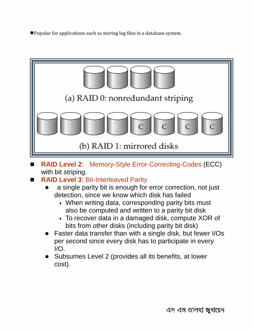
Popular for applications such as storing log files in a database system.
RAID Level 2: Memory-Style Error-Correcting-Codes (ECC) with bit striping.
RAID Level 3: Bit-Interleaved Parity a single parity bit is enough for error correction, not just
detection, since we know which disk has failed When writing data, corresponding parity bits must
also be computed and written to a parity bit disk To recover data in a damaged disk, compute XOR of
bits from other disks (including parity bit disk) Faster data transfer than with a single disk, but fewer I/Os
per second since every disk has to participate in every I/O.
Subsumes Level 2 (provides all its benefits, at lower cost).
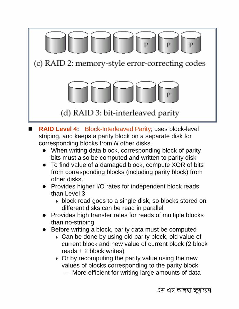
RAID Level 4: Block-Interleaved Parity; uses block-level striping, and keeps a parity block on a separate disk for corresponding blocks from N other disks. When writing data block, corresponding block of parity
bits must also be computed and written to parity disk To find value of a damaged block, compute XOR of bits
from corresponding blocks (including parity block) from other disks.
Provides higher I/O rates for independent block reads than Level 3 block read goes to a single disk, so blocks stored on
different disks can be read in parallel Provides high transfer rates for reads of multiple blocks
than no-striping Before writing a block, parity data must be computed
Can be done by using old parity block, old value of current block and new value of current block (2 block reads + 2 block writes)
Or by recomputing the parity value using the new values of blocks corresponding to the parity block
– More efficient for writing large amounts of data
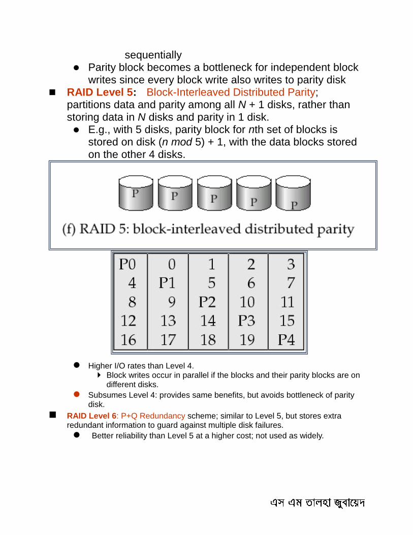
sequentially Parity block becomes a bottleneck for independent block
writes since every block write also writes to parity disk RAID Level 5: Block-Interleaved Distributed Parity;
partitions data and parity among all N + 1 disks, rather than storing data in N disks and parity in 1 disk. E.g., with 5 disks, parity block for nth set of blocks is
stored on disk (n mod 5) + 1, with the data blocks stored on the other 4 disks.
Higher I/O rates than Level 4. Block writes occur in parallel if the blocks and their parity blocks are on
different disks.
Subsumes Level 4: provides same benefits, but avoids bottleneck of parity disk.
RAID Level 6: P+Q Redundancy scheme; similar to Level 5, but stores extra redundant information to guard against multiple disk failures.
Better reliability than Level 5 at a higher cost; not used as widely.
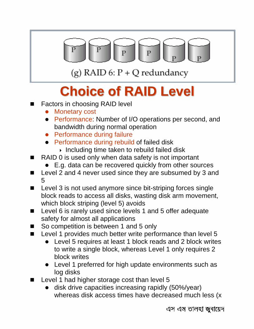
Choice of RAID Level Factors in choosing RAID level
Monetary cost Performance: Number of I/O operations per second, and
bandwidth during normal operation Performance during failure Performance during rebuild of failed disk
Including time taken to rebuild failed disk RAID 0 is used only when data safety is not important
E.g. data can be recovered quickly from other sources Level 2 and 4 never used since they are subsumed by 3 and
5 Level 3 is not used anymore since bit-striping forces single
block reads to access all disks, wasting disk arm movement, which block striping (level 5) avoids
Level 6 is rarely used since levels 1 and 5 offer adequate safety for almost all applications
So competition is between 1 and 5 only Level 1 provides much better write performance than level 5
Level 5 requires at least 1 block reads and 2 block writes to write a single block, whereas Level 1 only requires 2 block writes
Level 1 preferred for high update environments such as log disks
Level 1 had higher storage cost than level 5 disk drive capacities increasing rapidly (50%/year)
whereas disk access times have decreased much less (x

3 in 10 years) I/O requirements have increased greatly, e.g. for Web
servers When enough disks have been bought to satisfy required
rate of I/O, they often have spare storage capacity so there is often no extra monetary cost for Level 1!
Level 5 is preferred for applications with low update rate, and large amounts of data
Level 1 is preferred for all other applications
Hardware Issues Software RAID: RAID implementations done entirely in
software, with no special hardware support Hardware RAID: RAID implementations with special
hardware Use non-volatile RAM to record writes that are being
executed Beware: power failure during write can result in
corrupted disk E.g. failure after writing one block but before writing
the second in a mirrored system Such corrupted data must be detected when power is
restored – Recovery from corruption is similar to recovery
from failed disk – NV-RAM helps to efficiently detected potentially
corrupted blocks » Otherwise all blocks of disk must be read and
compared with mirror/parity block
Hot swapping: replacement of disk while system is running, without power down
Supported by some hardware RAID systems,
reduces time to recovery, and improves availability greatly
Many systems maintain spare disks which are kept online, and used as replacements for failed disks immediately on detection of failure

Reduces time to recovery greatly
Many hardware RAID systems ensure that a single point of failure will not stop the functioning of the system by using
Redundant power supplies with battery backup
Multiple controllers and multiple interconnections to guard against controller/interconnection failures
Storage Access A database file is partitioned into fixed-length storage units called blocks. Blocks
are units of both storage allocation and data transfer.
Database system seeks to minimize the number of block transfers between the disk and memory. We can reduce the number of disk accesses by keeping as many blocks as possible in main memory.
Buffer – portion of main memory available to store copies of disk blocks.
Buffer manager – subsystem responsible for allocating buffer space in main memory.
Buffer Manager Programs call on the buffer manager when they need a block from disk.
If the block is already in the buffer, buffer manager returns the address of the block in main memory
If the block is not in the buffer, the buffer manager
Allocates space in the buffer for the block
Replacing (throwing out) some other block, if required, to make space for the new block.
Replaced block written back to disk only if it was modified since the most recent time that it was written to/fetched from the disk.
Reads the block from the disk to the buffer, and returns the address of the block in main memory to requester.
Buffer-Replacement Policies Most operating systems replace the block least recently used (LRU strategy)
Idea behind LRU – use past pattern of block references as a predictor of future references
Queries have well-defined access patterns (such as sequential scans), and a database system can use the information in a user’s query to predict future references
LRU can be a bad strategy for certain access patterns involving repeated scans of data For example: when computing the join of 2 relations r and s by a nested
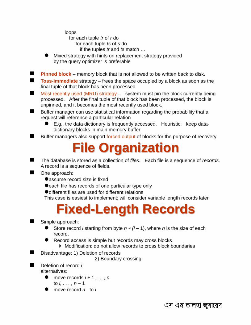
loops for each tuple tr of r do for each tuple ts of s do if the tuples tr and ts match …
Mixed strategy with hints on replacement strategy provided by the query optimizer is preferable
Pinned block – memory block that is not allowed to be written back to disk.
Toss-immediate strategy – frees the space occupied by a block as soon as the final tuple of that block has been processed
Most recently used (MRU) strategy – system must pin the block currently being processed. After the final tuple of that block has been processed, the block is unpinned, and it becomes the most recently used block.
Buffer manager can use statistical information regarding the probability that a request will reference a particular relation
E.g., the data dictionary is frequently accessed. Heuristic: keep data-dictionary blocks in main memory buffer
Buffer managers also support forced output of blocks for the purpose of recovery
File Organization The database is stored as a collection of files. Each file is a sequence of records.
A record is a sequence of fields.
One approach:
assume record size is fixed
each file has records of one particular type only
different files are used for different relations This case is easiest to implement; will consider variable length records later.
Fixed-Length Records Simple approach:
Store record i starting from byte n (i – 1), where n is the size of each record.
Record access is simple but records may cross blocks Modification: do not allow records to cross block boundaries
Disadvantage: 1) Deletion of records 2) Boundary crossing
Deletion of record i: alternatives:
move records i + 1, . . ., n to i, . . . , n – 1
move record n to i
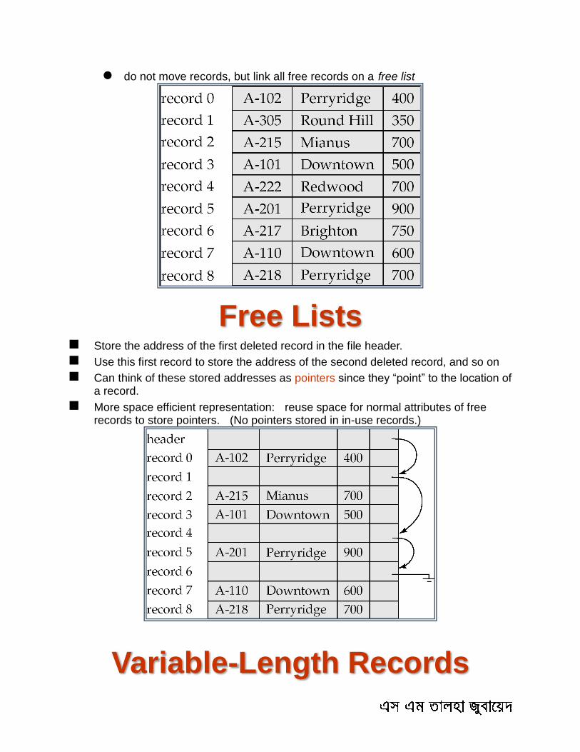
do not move records, but link all free records on a free list
Free Lists Store the address of the first deleted record in the file header.
Use this first record to store the address of the second deleted record, and so on
Can think of these stored addresses as pointers since they “point” to the location of a record.
More space efficient representation: reuse space for normal attributes of free records to store pointers. (No pointers stored in in-use records.)
Variable-Length Records
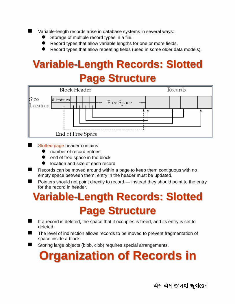
Variable-length records arise in database systems in several ways:
Storage of multiple record types in a file.
Record types that allow variable lengths for one or more fields.
Record types that allow repeating fields (used in some older data models).
Variable-Length Records: Slotted
Page Structure
Slotted page header contains:
number of record entries
end of free space in the block
location and size of each record
Records can be moved around within a page to keep them contiguous with no empty space between them; entry in the header must be updated.
Pointers should not point directly to record — instead they should point to the entry for the record in header.
Variable-Length Records: Slotted
Page Structure If a record is deleted, the space that it occupies is freed, and its entry is set to
deleted.
The level of indirection allows records to be moved to prevent fragmentation of space inside a block
Storing large objects (blob, clob) requires special arrangements.
Organization of Records in

Files Heap – a record can be placed anywhere in the file where there is space
Sequential – store records in sequential order, based on the value of the search key of each record
Hashing – a hash function computed on some attribute of each record; the result specifies in which block of the file the record should be placed
Records of each relation may be stored in a separate file. In a multitable clustering file organization records of several different relations can be stored in the same file
Motivation: store related records on the same block to minimize I/O
Sequential File Organization Suitable for applications that require sequential processing of the entire file
The records in the file are ordered by a search-key
Read in sorted order
Difficulty in insertion and deletion
Deletion – use pointer chains
Insertion –locate the position where the record is to be inserted
if there is free space insert there
if no free space, insert the record in an overflow block
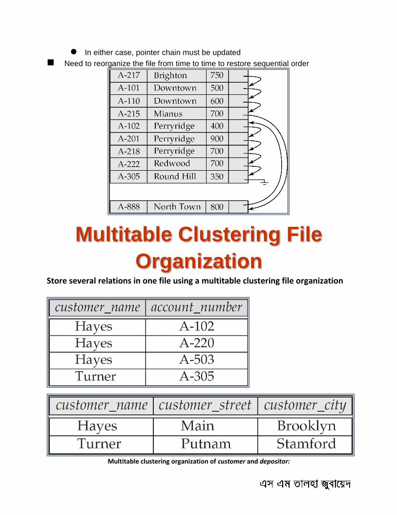
In either case, pointer chain must be updated
Need to reorganize the file from time to time to restore sequential order
Multitable Clustering File
Organization Store several relations in one file using a multitable clustering file organization
Multitable clustering organization of customer and depositor:
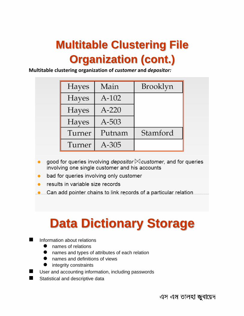
Multitable Clustering File
Organization (cont.) Multitable clustering organization of customer and depositor:
Data Dictionary Storage Information about relations
names of relations
names and types of attributes of each relation
names and definitions of views
integrity constraints
User and accounting information, including passwords
Statistical and descriptive data
number of tuples in each relation
Physical file organization information
How relation is stored (sequential/hash/…)
Physical location of relation
Information about indices
Catalog structure
Relational representation on disk
specialized data structures designed for efficient access, in memory
A possible catalog representation: Relation_metadata = (relation_name, number_of_attributes,
storage_organization, location) Attribute_metadata = (attribute_name, relation_name, domain_type, position, length) User_metadata = (user_name, encrypted_password, group) Index_metadata = (index_name, relation_name, index_type, index_attributes) View_metadata = (view_name, definition)

2014
11/16/2014

Indexing and Hashing Basic Concepts
Ordered Indices
B+-Tree Index Files
B-Tree Index Files
Static Hashing
Dynamic Hashing
Comparison of Ordered Indexing and Hashing
Index Definition in SQL
Multiple-Key Access
Basic Concepts Indexing mechanisms used to speed up access to desired data.
E.g., author catalog in library
Search Key - attribute to set of attributes used to look up records in a file.
An index file consists of records (called index entries) of the form
Index files are typically much smaller than the original file
Two basic kinds of indices:
Ordered indices: search keys are stored in sorted order
Hash indices: search keys are distributed uniformly across “buckets” using a “hash function”.
Index Evaluation Metrics Access types supported efficiently. E.g.,
records with a specified value in the attribute
or records with an attribute value falling in a specified range of values.
Access time
Insertion time
Deletion time
Space overhead
Ordered Indices In an ordered index, index entries are stored sorted on the search key value.
search-key pointer
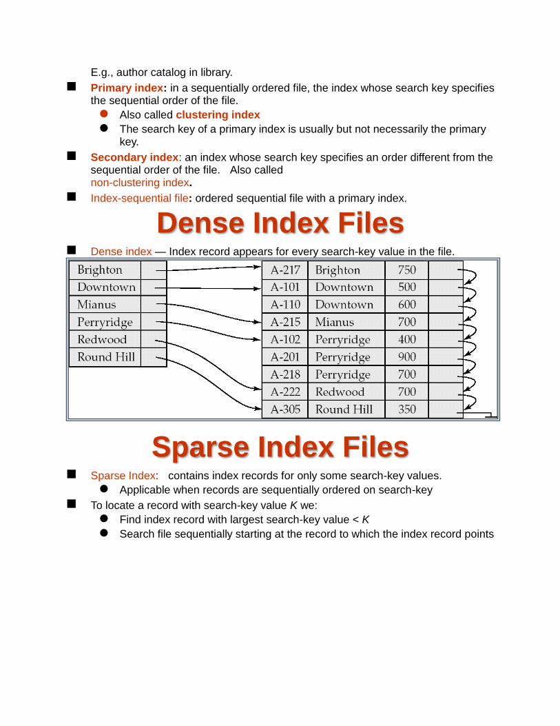
E.g., author catalog in library.
Primary index: in a sequentially ordered file, the index whose search key specifies the sequential order of the file.
Also called clustering index
The search key of a primary index is usually but not necessarily the primary key.
Secondary index: an index whose search key specifies an order different from the sequential order of the file. Also called non-clustering index.
Index-sequential file: ordered sequential file with a primary index.
Dense Index Files Dense index — Index record appears for every search-key value in the file.
Sparse Index Files Sparse Index: contains index records for only some search-key values.
Applicable when records are sequentially ordered on search-key
To locate a record with search-key value K we:
Find index record with largest search-key value < K
Search file sequentially starting at the record to which the index record points
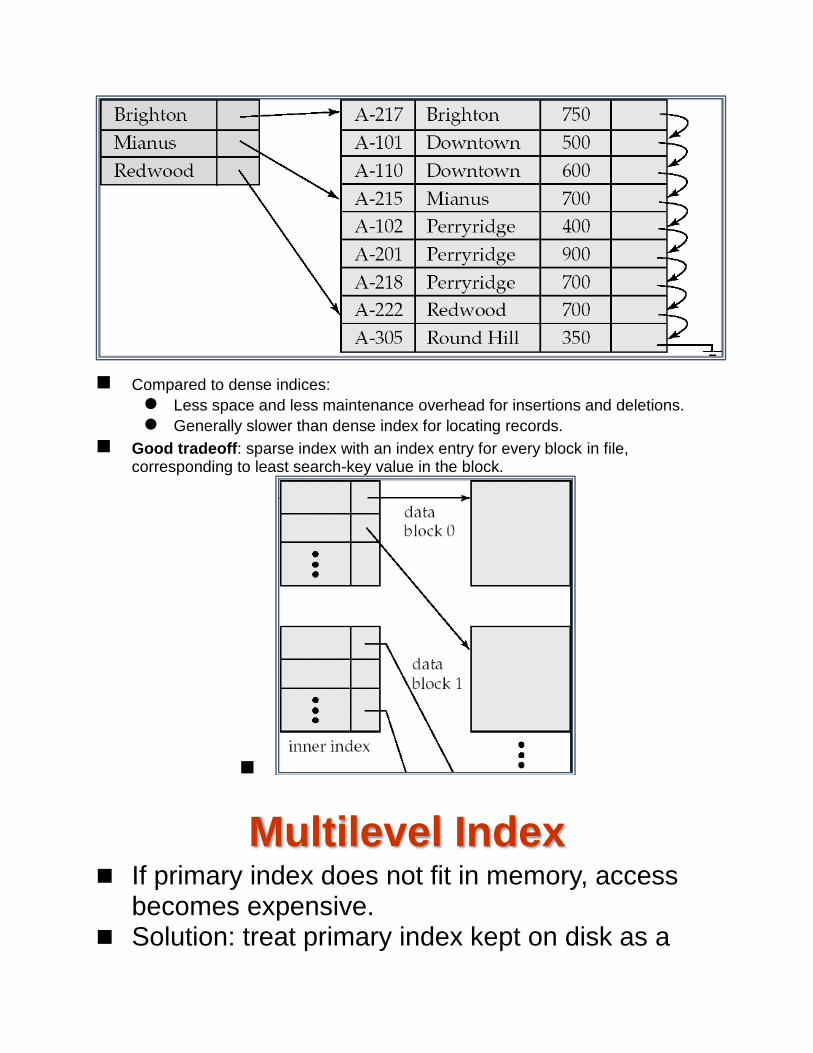
Compared to dense indices:
Less space and less maintenance overhead for insertions and deletions.
Generally slower than dense index for locating records.
Good tradeoff: sparse index with an index entry for every block in file, corresponding to least search-key value in the block.
Multilevel Index If primary index does not fit in memory, access
becomes expensive. Solution: treat primary index kept on disk as a

sequential file and construct a sparse index on it. outer index – a sparse index of primary index inner index – the primary index file
If even outer index is too large to fit in main memory, yet another level of index can be created, and so on.
Indices at all levels must be updated on insertion or deletion from the file.
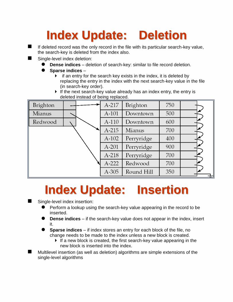
Index Update: Deletion If deleted record was the only record in the file with its particular search-key value,
the search-key is deleted from the index also.
Single-level index deletion:
Dense indices – deletion of search-key: similar to file record deletion.
Sparse indices – if an entry for the search key exists in the index, it is deleted by
replacing the entry in the index with the next search-key value in the file (in search-key order).
If the next search-key value already has an index entry, the entry is deleted instead of being replaced.
Index Update: Insertion Single-level index insertion:
Perform a lookup using the search-key value appearing in the record to be inserted.
Dense indices – if the search-key value does not appear in the index, insert it.
Sparse indices – if index stores an entry for each block of the file, no change needs to be made to the index unless a new block is created. If a new block is created, the first search-key value appearing in the
new block is inserted into the index.
Multilevel insertion (as well as deletion) algorithms are simple extensions of the single-level algorithms
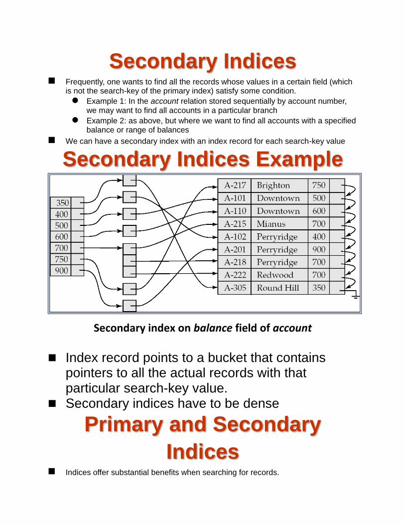
Secondary Indices Frequently, one wants to find all the records whose values in a certain field (which
is not the search-key of the primary index) satisfy some condition.
Example 1: In the account relation stored sequentially by account number, we may want to find all accounts in a particular branch
Example 2: as above, but where we want to find all accounts with a specified balance or range of balances
We can have a secondary index with an index record for each search-key value
Secondary Indices Example
Secondary index on balance field of account
Index record points to a bucket that contains pointers to all the actual records with that particular search-key value.
Secondary indices have to be dense
Primary and Secondary
Indices Indices offer substantial benefits when searching for records.

BUT: Updating indices imposes overhead on database modification --when a file is modified, every index on the file must be updated,
Sequential scan using primary index is efficient, but a sequential scan using a secondary index is expensive
Each record access may fetch a new block from disk
Block fetch requires about 5 to 10 micro seconds, versus about 100 nanoseconds for memory access
B+-Tree Index Files B+-tree indices are an alternative to indexed-sequential files.
Disadvantage of indexed-sequential files
performance degrades as file grows, since many overflow blocks get created.
Periodic reorganization of entire file is required.
Advantage of B+-tree index files:
automatically reorganizes itself with small, local, changes, in the face of insertions and deletions.
Reorganization of entire file is not required to maintain performance.
(Minor) disadvantage of B+-trees:
extra insertion and deletion overhead, space overhead.
Advantages of B+-trees outweigh disadvantages
B+-trees are used extensively
All paths from root to leaf are of the same length
Each node that is not a root or a leaf has between n/2 and n children.
A leaf node has between (n–1)/2 and n–1 values
Special cases:
If the root is not a leaf, it has at least 2 children.
If the root is a leaf (that is, there are no other nodes in the tree), it can have between 0 and (n–1) values.
B+-Tree Node Structure Typical node
Ki are the search-key values
Pi are pointers to children (for non-leaf nodes) or pointers to records or
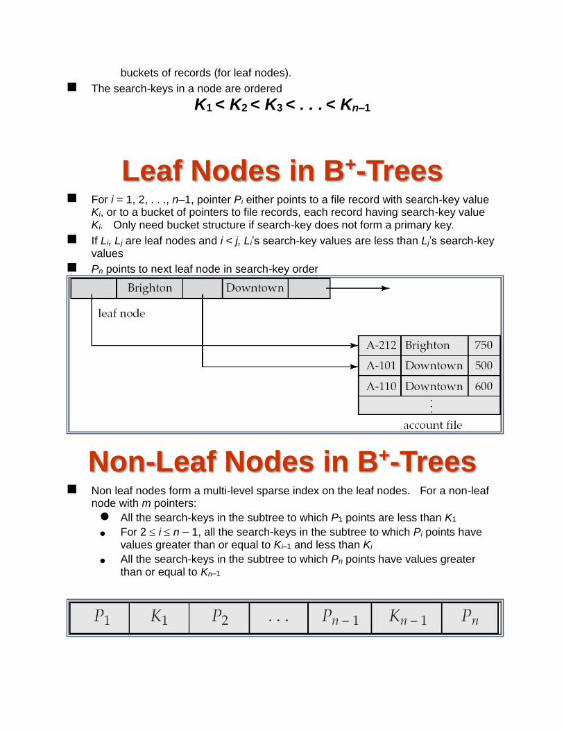
buckets of records (for leaf nodes).
The search-keys in a node are ordered
K1 < K2 < K3 < . . . < Kn–1
Leaf Nodes in B+-Trees For i = 1, 2, . . ., n–1, pointer Pi either points to a file record with search-key value
Ki, or to a bucket of pointers to file records, each record having search-key value Ki. Only need bucket structure if search-key does not form a primary key.
If Li, Lj are leaf nodes and i < j, Li’s search-key values are less than Lj’s search-key values
Pn points to next leaf node in search-key order
Non-Leaf Nodes in B+-Trees Non leaf nodes form a multi-level sparse index on the leaf nodes. For a non-leaf
node with m pointers:
All the search-keys in the subtree to which P1 points are less than K1
For 2 i n – 1, all the search-keys in the subtree to which Pi points have values greater than or equal to Ki–1 and less than Ki
All the search-keys in the subtree to which Pn points have values greater than or equal to Kn–1
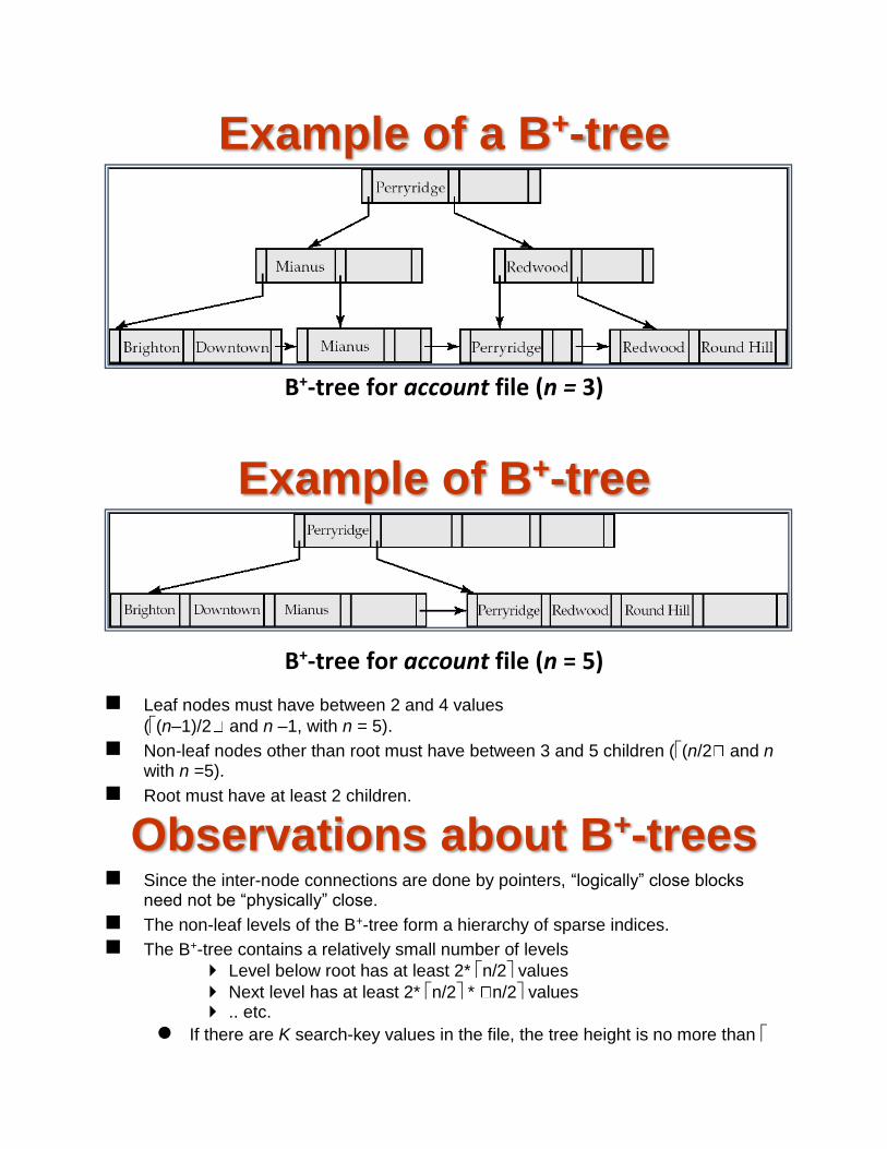
Example of a B+-tree
B+-tree for account file (n = 3)
Example of B+-tree
B+-tree for account file (n = 5)
Leaf nodes must have between 2 and 4 values
((n–1)/2 and n –1, with n = 5).
Non-leaf nodes other than root must have between 3 and 5 children ((n/2 and n with n =5).
Root must have at least 2 children.
Observations about B+-trees Since the inter-node connections are done by pointers, “logically” close blocks
need not be “physically” close.
The non-leaf levels of the B+-tree form a hierarchy of sparse indices.
The B+-tree contains a relatively small number of levels
Level below root has at least 2* n/2 values
Next level has at least 2* n/2 * n/2 values .. etc.
If there are K search-key values in the file, the tree height is no more than
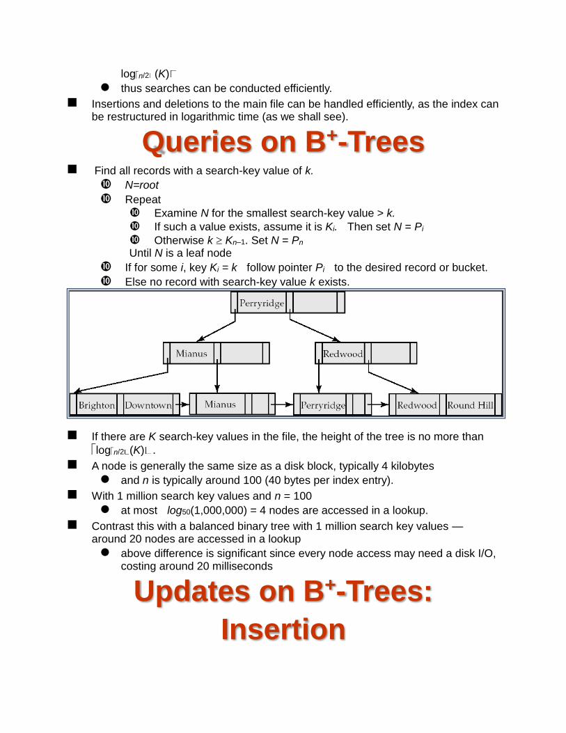
logn/2 (K)
thus searches can be conducted efficiently.
Insertions and deletions to the main file can be handled efficiently, as the index can be restructured in logarithmic time (as we shall see).
Queries on B+-Trees Find all records with a search-key value of k.
N=root
Repeat
Examine N for the smallest search-key value > k.
If such a value exists, assume it is Ki. Then set N = Pi
Otherwise k Kn–1. Set N = Pn Until N is a leaf node
If for some i, key Ki = k follow pointer Pi to the desired record or bucket.
Else no record with search-key value k exists.
If there are K search-key values in the file, the height of the tree is no more than
logn/2 (K) .
A node is generally the same size as a disk block, typically 4 kilobytes
and n is typically around 100 (40 bytes per index entry).
With 1 million search key values and n = 100
at most log50(1,000,000) = 4 nodes are accessed in a lookup.
Contrast this with a balanced binary tree with 1 million search key values — around 20 nodes are accessed in a lookup
above difference is significant since every node access may need a disk I/O, costing around 20 milliseconds
Updates on B+-Trees:
Insertion
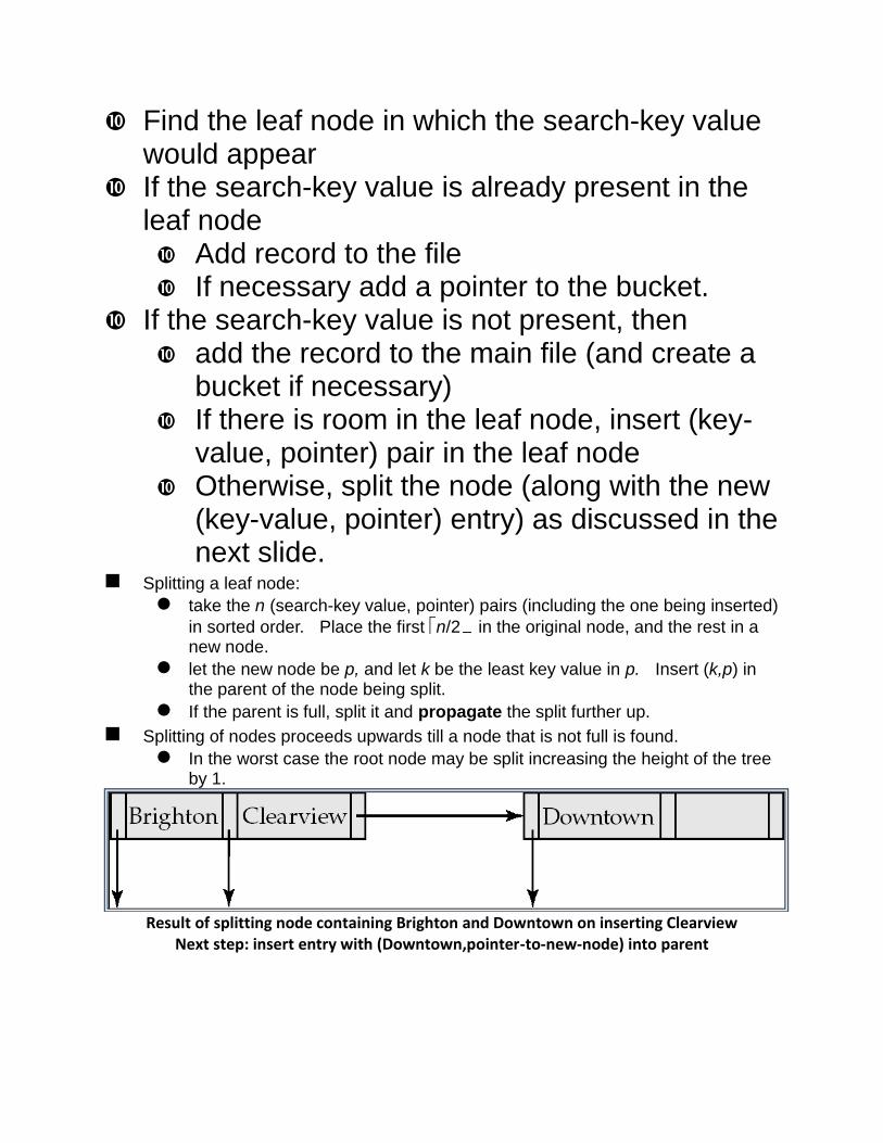
Find the leaf node in which the search-key value would appear
If the search-key value is already present in the leaf node Add record to the file If necessary add a pointer to the bucket.
If the search-key value is not present, then add the record to the main file (and create a
bucket if necessary) If there is room in the leaf node, insert (key-
value, pointer) pair in the leaf node Otherwise, split the node (along with the new
(key-value, pointer) entry) as discussed in the next slide.
Splitting a leaf node:
take the n (search-key value, pointer) pairs (including the one being inserted)
in sorted order. Place the first n/2 in the original node, and the rest in a new node.
let the new node be p, and let k be the least key value in p. Insert (k,p) in the parent of the node being split.
If the parent is full, split it and propagate the split further up.
Splitting of nodes proceeds upwards till a node that is not full is found.
In the worst case the root node may be split increasing the height of the tree by 1.
Result of splitting node containing Brighton and Downtown on inserting Clearview
Next step: insert entry with (Downtown,pointer-to-new-node) into parent

B+-Tree before and after insertion of “Clearview”
Splitting a non-leaf node: when inserting (k,p) into an already full internal node N
Copy N to an in-memory area M with space for n+1 pointers and n keys
Insert (k,p) into M
Copy P1,K1, …, K n/2-1,P n/2 from M back into node N
Copy Pn/2+1,K n/2+1,…,Kn,Pn+1 from M into newly allocated node N’
Insert (K n/2,N’) into parent N
Read pseudocode in book!
Updates on B+-Trees: Deletion Find the record to be deleted, and remove it from the main file and from the bucket
(if present)
Remove (search-key value, pointer) from the leaf node if there is no bucket or if the
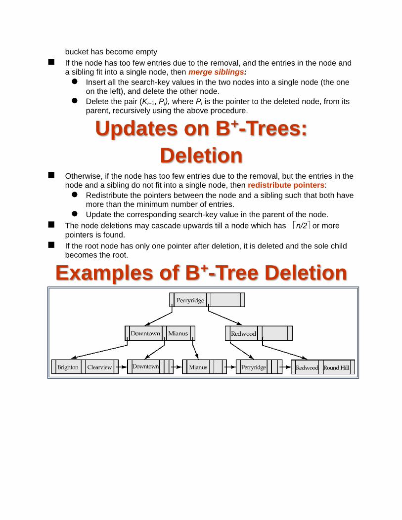
bucket has become empty
If the node has too few entries due to the removal, and the entries in the node and a sibling fit into a single node, then merge siblings:
Insert all the search-key values in the two nodes into a single node (the one on the left), and delete the other node.
Delete the pair (Ki–1, Pi), where Pi is the pointer to the deleted node, from its parent, recursively using the above procedure.
Updates on B+-Trees:
Deletion Otherwise, if the node has too few entries due to the removal, but the entries in the
node and a sibling do not fit into a single node, then redistribute pointers:
Redistribute the pointers between the node and a sibling such that both have more than the minimum number of entries.
Update the corresponding search-key value in the parent of the node.
The node deletions may cascade upwards till a node which has n/2 or more pointers is found.
If the root node has only one pointer after deletion, it is deleted and the sole child becomes the root.
Examples of B+-Tree Deletion

Before and after deleting “Downtown”
Deleting “Downtown” causes merging of under-full leaves
leaf node can become empty only for n=3!
Deletion of “Perryridge” from result of previous example
Leaf with “Perryridge” becomes underfull (actually empty, in this special case) and merged with its sibling.
As a result “Perryridge” node’s parent became underfull, and was merged with its sibling Value separating two nodes (at parent) moves into merged node Entry deleted from parent
Root node then has only one child, and is deleted
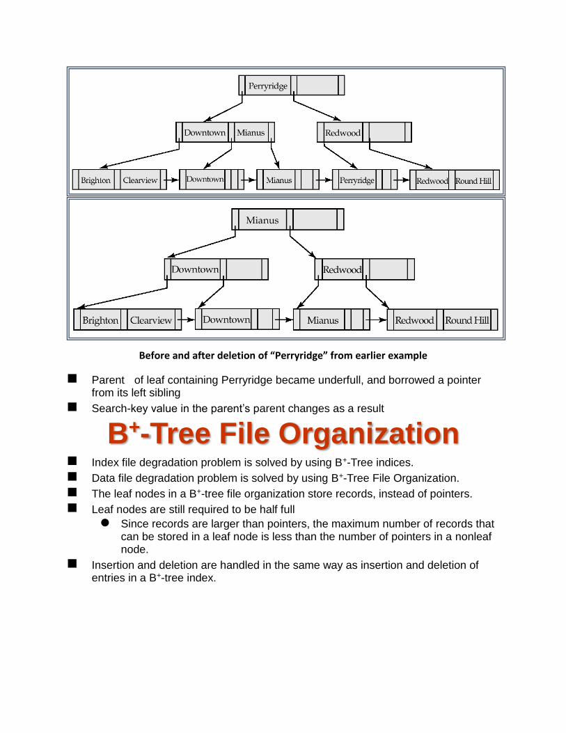
Before and after deletion of “Perryridge” from earlier example
Parent of leaf containing Perryridge became underfull, and borrowed a pointer from its left sibling
Search-key value in the parent’s parent changes as a result
B+-Tree File Organization Index file degradation problem is solved by using B+-Tree indices.
Data file degradation problem is solved by using B+-Tree File Organization.
The leaf nodes in a B+-tree file organization store records, instead of pointers.
Leaf nodes are still required to be half full
Since records are larger than pointers, the maximum number of records that can be stored in a leaf node is less than the number of pointers in a nonleaf node.
Insertion and deletion are handled in the same way as insertion and deletion of entries in a B+-tree index.
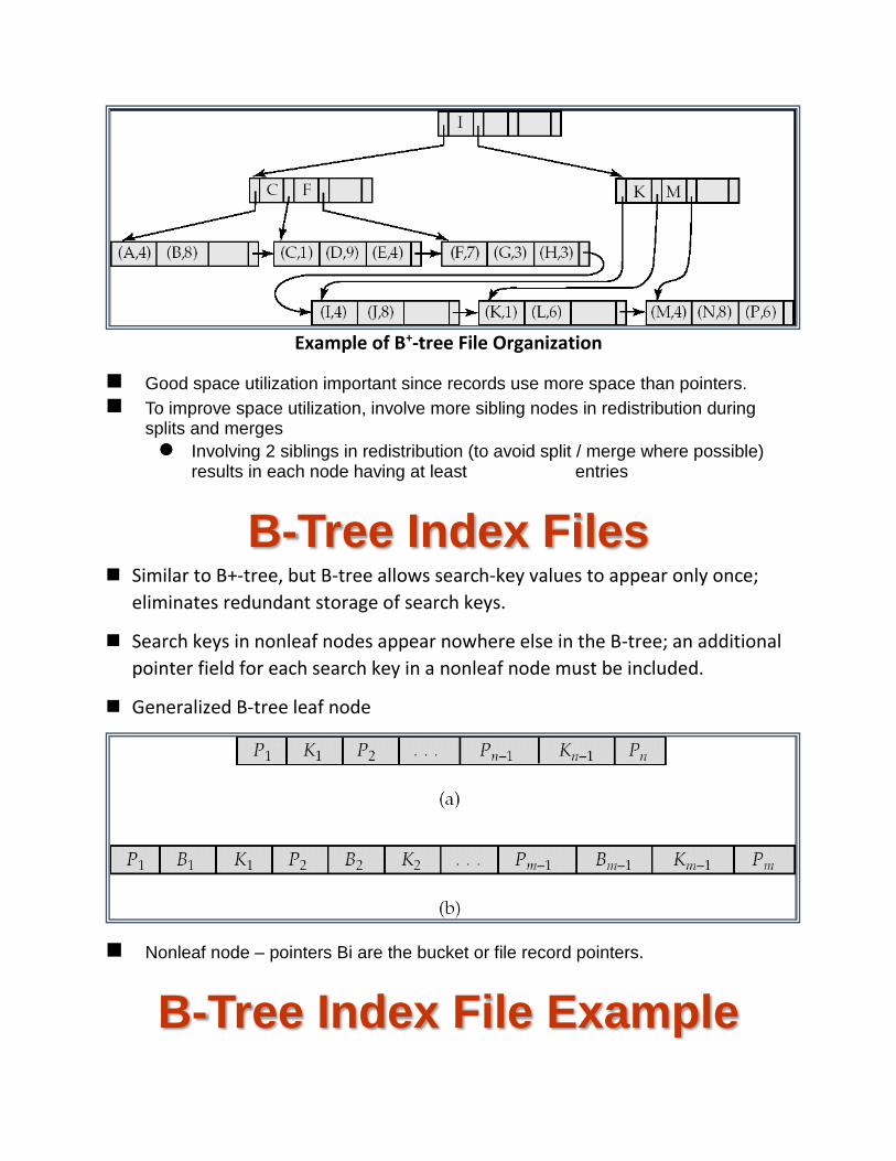
Example of B+-tree File Organization
Good space utilization important since records use more space than pointers.
To improve space utilization, involve more sibling nodes in redistribution during splits and merges
Involving 2 siblings in redistribution (to avoid split / merge where possible) results in each node having at least entries
B-Tree Index Files Similar to B+-tree, but B-tree allows search-key values to appear only once;
eliminates redundant storage of search keys.
Search keys in nonleaf nodes appear nowhere else in the B-tree; an additional
pointer field for each search key in a nonleaf node must be included.
Generalized B-tree leaf node
Nonleaf node – pointers Bi are the bucket or file record pointers.
B-Tree Index File Example

B-tree (above) and B+-tree (below) on same data
Advantages of B-Tree indices:
May use less tree nodes than a corresponding B+-Tree.
Sometimes possible to find search-key value before reaching leaf node.
Disadvantages of B-Tree indices:
Only small fraction of all search-key values are found early
Non-leaf nodes are larger, so fan-out is reduced. Thus, B-Trees typically have greater depth than corresponding B+-Tree
Insertion and deletion more complicated than in B+-Trees
Implementation is harder than B+-Trees.
Typically, advantages of B-Trees do not out weigh disadvantages.
Multiple-Key Access Use multiple indices for certain types of queries.
Example: select account_number from account where branch_name = “Perryridge” and balance = 1000
Possible strategies for processing query using indices on single attributes:
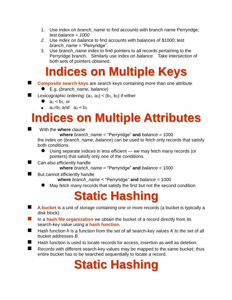
1. Use index on branch_name to find accounts with branch name Perryridge; test balance = 1000
2. Use index on balance to find accounts with balances of $1000; test branch_name = “Perryridge”.
3. Use branch_name index to find pointers to all records pertaining to the Perryridge branch. Similarly use index on balance. Take intersection of both sets of pointers obtained.
Indices on Multiple Keys Composite search keys are search keys containing more than one attribute
E.g. (branch_name, balance)
Lexicographic ordering: (a1, a2) < (b1, b2) if either
a1 < b1, or
a1=b1 and a2 < b2
Indices on Multiple Attributes With the where clause
where branch_name = “Perryridge” and balance = 1000 the index on (branch_name, balance) can be used to fetch only records that satisfy both conditions.
Using separate indices in less efficient — we may fetch many records (or pointers) that satisfy only one of the conditions.
Can also efficiently handle where branch_name = “Perryridge” and balance < 1000
But cannot efficiently handle where branch_name < “Perryridge” and balance = 1000
May fetch many records that satisfy the first but not the second condition
Static Hashing A bucket is a unit of storage containing one or more records (a bucket is typically a
disk block).
In a hash file organization we obtain the bucket of a record directly from its search-key value using a hash function.
Hash function h is a function from the set of all search-key values K to the set of all bucket addresses B.
Hash function is used to locate records for access, insertion as well as deletion.
Records with different search-key values may be mapped to the same bucket; thus entire bucket has to be searched sequentially to locate a record.
Static Hashing
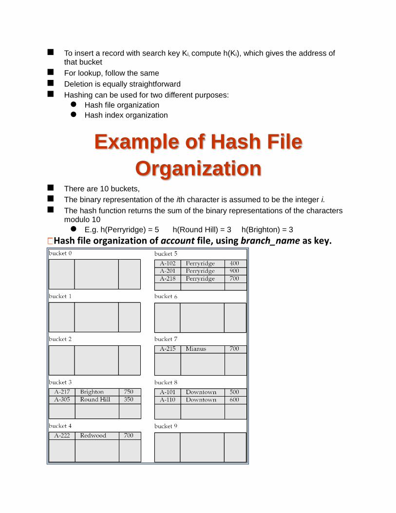
To insert a record with search key Ki, compute h(Ki), which gives the address of that bucket
For lookup, follow the same
Deletion is equally straightforward
Hashing can be used for two different purposes:
Hash file organization
Hash index organization
Example of Hash File
Organization There are 10 buckets,
The binary representation of the ith character is assumed to be the integer i.
The hash function returns the sum of the binary representations of the characters modulo 10
E.g. h(Perryridge) = 5 h(Round Hill) = 3 h(Brighton) = 3
Hash file organization of account file, using branch_name as key.
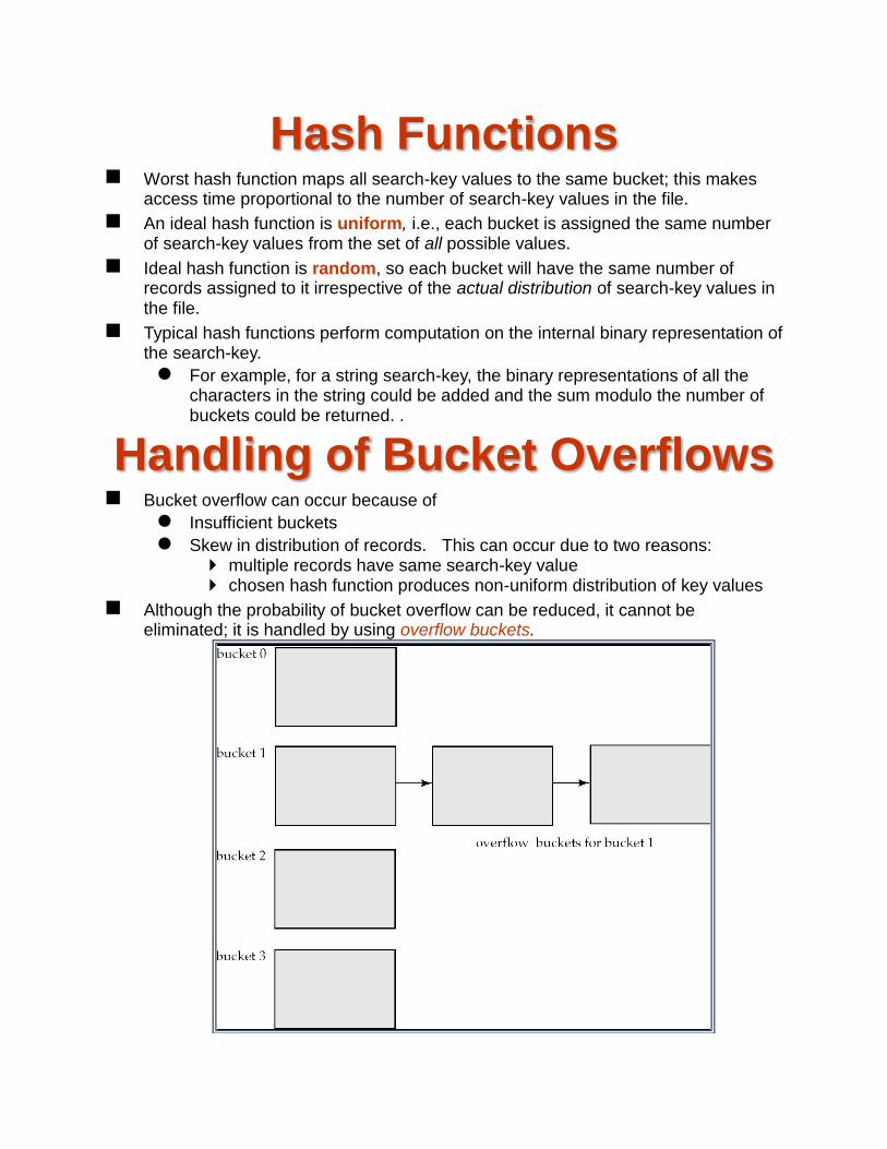
Hash Functions Worst hash function maps all search-key values to the same bucket; this makes
access time proportional to the number of search-key values in the file.
An ideal hash function is uniform, i.e., each bucket is assigned the same number of search-key values from the set of all possible values.
Ideal hash function is random, so each bucket will have the same number of records assigned to it irrespective of the actual distribution of search-key values in the file.
Typical hash functions perform computation on the internal binary representation of the search-key.
For example, for a string search-key, the binary representations of all the characters in the string could be added and the sum modulo the number of buckets could be returned. .
Handling of Bucket Overflows Bucket overflow can occur because of
Insufficient buckets
Skew in distribution of records. This can occur due to two reasons: multiple records have same search-key value chosen hash function produces non-uniform distribution of key values
Although the probability of bucket overflow can be reduced, it cannot be eliminated; it is handled by using overflow buckets.
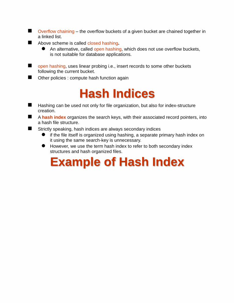
Overflow chaining – the overflow buckets of a given bucket are chained together in a linked list.
Above scheme is called closed hashing.
An alternative, called open hashing, which does not use overflow buckets, is not suitable for database applications.
open hashing, uses linear probing i.e., insert records to some other buckets following the current bucket.
Other policies : compute hash function again
Hash Indices Hashing can be used not only for file organization, but also for index-structure
creation.
A hash index organizes the search keys, with their associated record pointers, into a hash file structure.
Strictly speaking, hash indices are always secondary indices
if the file itself is organized using hashing, a separate primary hash index on it using the same search-key is unnecessary.
However, we use the term hash index to refer to both secondary index structures and hash organized files.
Example of Hash Index
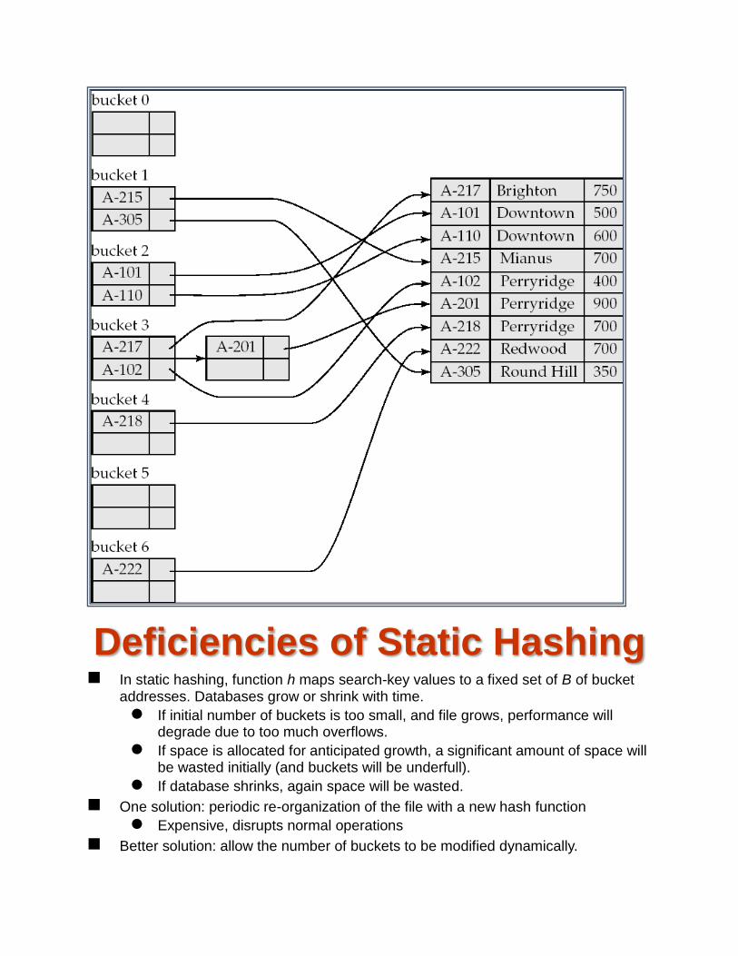
Deficiencies of Static Hashing In static hashing, function h maps search-key values to a fixed set of B of bucket
addresses. Databases grow or shrink with time.
If initial number of buckets is too small, and file grows, performance will degrade due to too much overflows.
If space is allocated for anticipated growth, a significant amount of space will be wasted initially (and buckets will be underfull).
If database shrinks, again space will be wasted.
One solution: periodic re-organization of the file with a new hash function
Expensive, disrupts normal operations
Better solution: allow the number of buckets to be modified dynamically.

Dynamic Hashing Good for database that grows and shrinks in size
Allows the hash function to be modified dynamically
Extendable hashing – one form of dynamic hashing
Hash function generates values over a large range — typically b-bit integers, with b = 32.
At any time use only a prefix of the hash function to index into a table of bucket addresses.
Let the length of the prefix be i bits, 0 i 32.
Bucket address table size = 2i. Initially i = 0
Value of i grows and shrinks as the size of the database grows and shrinks.
Multiple entries in the bucket address table may point to a bucket (why?)
Thus, actual number of buckets is < 2i
The number of buckets also changes dynamically due to coalescing and splitting of buckets.
General Extendable Hash
Structure
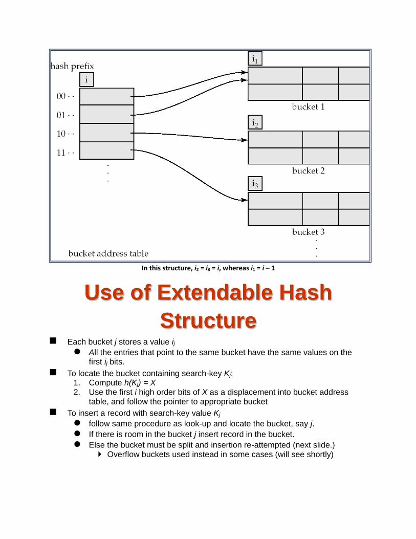
In this structure, i2 = i3 = i, whereas i1 = i – 1
Use of Extendable Hash
Structure Each bucket j stores a value ij
All the entries that point to the same bucket have the same values on the first ij bits.
To locate the bucket containing search-key Kj: 1. Compute h(Kj) = X 2. Use the first i high order bits of X as a displacement into bucket address
table, and follow the pointer to appropriate bucket
To insert a record with search-key value Kj
follow same procedure as look-up and locate the bucket, say j.
If there is room in the bucket j insert record in the bucket.
Else the bucket must be split and insertion re-attempted (next slide.) Overflow buckets used instead in some cases (will see shortly)
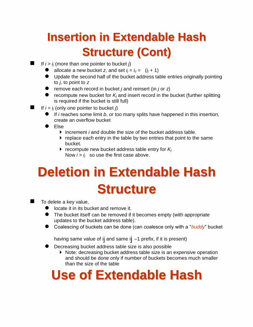
Insertion in Extendable Hash
Structure (Cont) If i > ij (more than one pointer to bucket j)
allocate a new bucket z, and set ij = iz = (ij + 1)
Update the second half of the bucket address table entries originally pointing to j, to point to z
remove each record in bucket j and reinsert (in j or z)
recompute new bucket for Kj and insert record in the bucket (further splitting is required if the bucket is still full)
If i = ij (only one pointer to bucket j)
If i reaches some limit b, or too many splits have happened in this insertion, create an overflow bucket
Else increment i and double the size of the bucket address table. replace each entry in the table by two entries that point to the same
bucket. recompute new bucket address table entry for Kj
Now i > ij so use the first case above.
Deletion in Extendable Hash
Structure To delete a key value,
locate it in its bucket and remove it.
The bucket itself can be removed if it becomes empty (with appropriate updates to the bucket address table).
Coalescing of buckets can be done (can coalesce only with a “buddy” bucket
having same value of ij and same ij –1 prefix, if it is present)
Decreasing bucket address table size is also possible Note: decreasing bucket address table size is an expensive operation
and should be done only if number of buckets becomes much smaller than the size of the table
Use of Extendable Hash
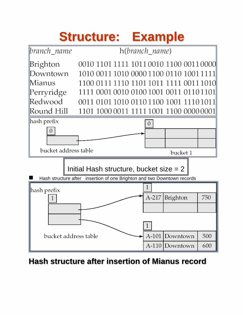
Structure: Example
Hash structure after insertion of one Brighton and two Downtown records
Hash structure after insertion of Mianus record
Initial Hash structure, bucket size = 2
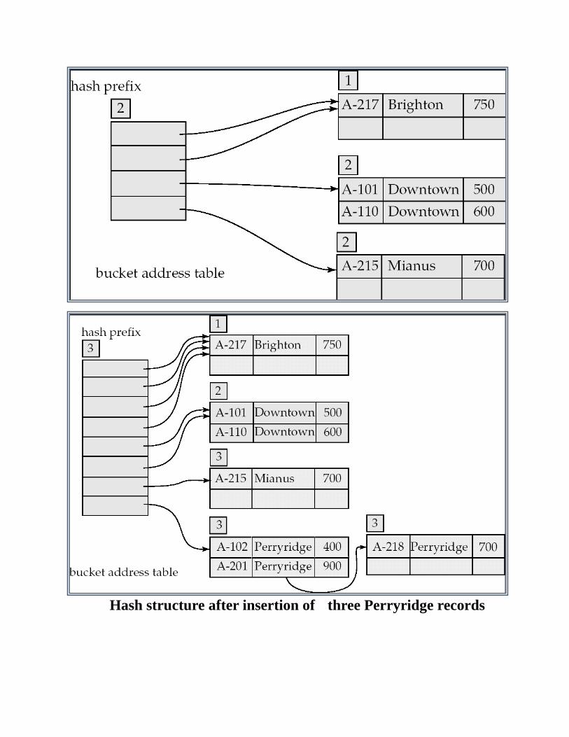
Hash structure after insertion of three Perryridge records
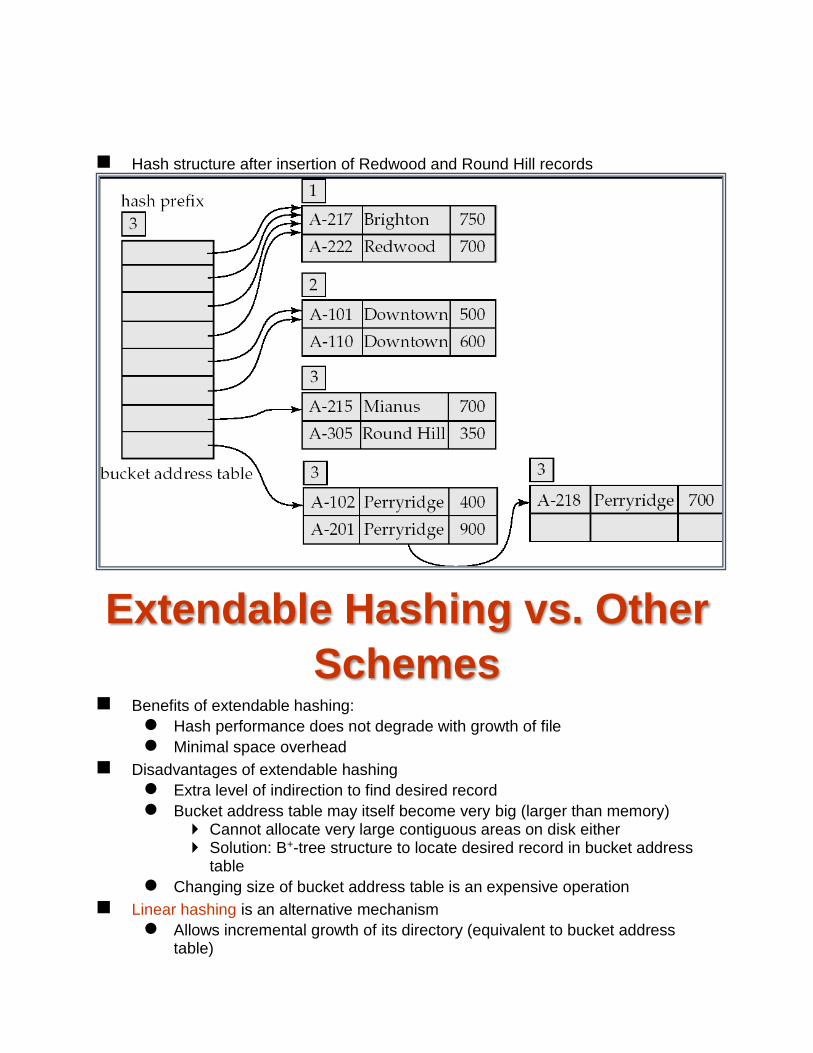
Hash structure after insertion of Redwood and Round Hill records
Extendable Hashing vs. Other
Schemes Benefits of extendable hashing:
Hash performance does not degrade with growth of file
Minimal space overhead
Disadvantages of extendable hashing
Extra level of indirection to find desired record
Bucket address table may itself become very big (larger than memory) Cannot allocate very large contiguous areas on disk either Solution: B+-tree structure to locate desired record in bucket address
table
Changing size of bucket address table is an expensive operation
Linear hashing is an alternative mechanism
Allows incremental growth of its directory (equivalent to bucket address table)
At the cost of more bucket overflows
Comparison of Ordered Indexing
and Hashing Selection of Indexing Technique: Cost of periodic re-organization
Relative frequency of insertions and deletions
Is it desirable to optimize average access time at the expense of worst-case access time?
Expected type of queries:
Hashing is generally better at retrieving records having a specified value of the key.
If range queries are common, ordered indices are to be preferred
In practice:
PostgreSQL supports hash indices, but discourages use due to poor performance
Oracle supports static hash organization, but not hash indices
SQLServer supports only B+-trees
Bitmap Indices Bitmap indices are a special type of index designed for efficient querying on
multiple keys
Records in a relation are assumed to be numbered sequentially from, say, 0
Given a number n it must be easy to retrieve record n Particularly easy if records are of fixed size
Applicable on attributes that take on a relatively small number of distinct values
E.g. gender, country, state, …
E.g. income-level (income broken up into a small number of levels such as 0-9999, 10000-19999, 20000-50000, 50000- infinity)
A bitmap is simply an array of bits
In its simplest form a bitmap index on an attribute has a bitmap for each value of the attribute
Bitmap has as many bits as records
In a bitmap for value v, the bit for a record is 1 if the record has the value v for the attribute, and is 0 otherwise

Bitmap indices are useful for queries on multiple attributes
not particularly useful for single attribute queries
Queries are answered using bitmap operations
Intersection (and)
Union (or)
Complementation (not)
Each operation takes two bitmaps of the same size and applies the operation on corresponding bits to get the result bitmap
E.g. 100110 AND 110011 = 100010 100110 OR 110011 = 110111
NOT 100110 = 011001
Males with income level L1: 10010 AND 10100 = 10000 Can then retrieve required tuples. Counting number of matching tuples is even faster
Bitmap indices generally very small compared with relation size
E.g. if record is 100 bytes, space for a single bitmap is 1/800 of space used by relation. If number of distinct attribute values is 8, bitmap is only 1% of relation
size
Deletion needs to be handled properly
Existence bitmap to note if there is a valid record at a record location
Needed for complementation
Efficient Implementation of Bitmap
Operations Bitmaps are packed into words; a single word and (a basic CPU instruction)
computes and of 32 or 64 bits at once
E.g. 1-million-bit maps can be and-ed with just 31,250 instruction
Counting number of 1s can be done fast by a trick:

Use each byte to index into a pre-computed array of 256 elements each storing the count of 1s in the binary representation Can use pairs of bytes to speed up further at a higher memory cost
Add up the retrieved counts