msc economics economic theory and applications i microeconomics · msc economics economic theory...
TRANSCRIPT

MSc Economics
Economic Theory and Applications I
Microeconomics
Dr Ken Hori, [email protected]
Birkbeck College, University of London
October 2006

Contents
1 Theory of Choice: An Axiomatic Approach 11.1 Consumer Choice . . . . . . . . . . . . . . . . . . . . . . . . . . . . . . . . . 11.2 Preference Relations . . . . . . . . . . . . . . . . . . . . . . . . . . . . . . . 21.3 Ordering of Bundles . . . . . . . . . . . . . . . . . . . . . . . . . . . . . . . 21.4 Utility Function . . . . . . . . . . . . . . . . . . . . . . . . . . . . . . . . . . 41.5 Example: Lexicographic Preference Relation . . . . . . . . . . . . . . . . . . 51.6 Appendix . . . . . . . . . . . . . . . . . . . . . . . . . . . . . . . . . . . . . 6
2 Consumer Theory 72.1 Utility Maximisation Problem . . . . . . . . . . . . . . . . . . . . . . . . . . 72.2 Expenditure Minimisation Problem . . . . . . . . . . . . . . . . . . . . . . . 102.3 Duality Theory . . . . . . . . . . . . . . . . . . . . . . . . . . . . . . . . . . 122.4 Slutsky Decomposition . . . . . . . . . . . . . . . . . . . . . . . . . . . . . . 122.5 Welfare Measurement . . . . . . . . . . . . . . . . . . . . . . . . . . . . . . 14
2.5.1 Money Metric Utility Functions . . . . . . . . . . . . . . . . . . . . . 152.5.2 Compensating and Equivalent Variations . . . . . . . . . . . . . . . 152.5.3 Consumer Surplus as an Approximation . . . . . . . . . . . . . . . . 16
2.6 Aggregation Issue . . . . . . . . . . . . . . . . . . . . . . . . . . . . . . . . . 182.7 Application: Neoclassical Model of Labour Supply . . . . . . . . . . . . . . 202.8 Example . . . . . . . . . . . . . . . . . . . . . . . . . . . . . . . . . . . . . . 212.9 Appendix . . . . . . . . . . . . . . . . . . . . . . . . . . . . . . . . . . . . . 24
2.9.1 Quasi-Concavity and Quasi-Convexity . . . . . . . . . . . . . . . . . 242.9.2 Envelope Theorem . . . . . . . . . . . . . . . . . . . . . . . . . . . . 262.9.3 Quasilinear Utility Function . . . . . . . . . . . . . . . . . . . . . . . 272.9.4 Homogeneous and Homothetic Utility Functions . . . . . . . . . . . 28
3 Producer Theory 303.1 Technology . . . . . . . . . . . . . . . . . . . . . . . . . . . . . . . . . . . . 303.2 Possible Restrictions on Technology Set . . . . . . . . . . . . . . . . . . . . 313.3 Technical Rate of Substitution . . . . . . . . . . . . . . . . . . . . . . . . . 313.4 Returns to Scale . . . . . . . . . . . . . . . . . . . . . . . . . . . . . . . . . 313.5 Profit Maximisation Problem . . . . . . . . . . . . . . . . . . . . . . . . . . 32
3.5.1 Demand and Supply Functions . . . . . . . . . . . . . . . . . . . . . 32

i
3.5.2 Profit Function . . . . . . . . . . . . . . . . . . . . . . . . . . . . . . 343.5.3 Example . . . . . . . . . . . . . . . . . . . . . . . . . . . . . . . . . . 36
3.6 Cost Minimisation Problem . . . . . . . . . . . . . . . . . . . . . . . . . . . 383.6.1 Example: Cobb-Douglas Technology . . . . . . . . . . . . . . . . . . 413.6.2 Example: Leontief Technology . . . . . . . . . . . . . . . . . . . . . 423.6.3 Example: Linear Technology . . . . . . . . . . . . . . . . . . . . . . 43
3.7 Duality . . . . . . . . . . . . . . . . . . . . . . . . . . . . . . . . . . . . . . 433.7.1 Example: Leontief Technology . . . . . . . . . . . . . . . . . . . . . 44
3.8 Aggregation . . . . . . . . . . . . . . . . . . . . . . . . . . . . . . . . . . . . 45
4 Monopoly 474.1 Monopoly Profit Maximisation . . . . . . . . . . . . . . . . . . . . . . . . . 47
4.1.1 Example: Linear Demand . . . . . . . . . . . . . . . . . . . . . . . . 484.2 Monopoly Inefficiency . . . . . . . . . . . . . . . . . . . . . . . . . . . . . . 484.3 Price Discrimination . . . . . . . . . . . . . . . . . . . . . . . . . . . . . . . 50
4.3.1 First-degree Price Discrimination . . . . . . . . . . . . . . . . . . . . 504.3.2 Second-degree Price Discrimination . . . . . . . . . . . . . . . . . . . 514.3.3 Third-degree Price Discrimination . . . . . . . . . . . . . . . . . . . 53
5 Choice under Uncertainty 545.1 Lotteries . . . . . . . . . . . . . . . . . . . . . . . . . . . . . . . . . . . . . . 545.2 Preferences over Lotteries . . . . . . . . . . . . . . . . . . . . . . . . . . . . 555.3 Example: The Demand for Insurance . . . . . . . . . . . . . . . . . . . . . . 585.4 Allais Paradox (1953) . . . . . . . . . . . . . . . . . . . . . . . . . . . . . . 595.5 Risk Aversion . . . . . . . . . . . . . . . . . . . . . . . . . . . . . . . . . . . 605.6 Example . . . . . . . . . . . . . . . . . . . . . . . . . . . . . . . . . . . . . . 625.7 Comparison of Return and Riskiness . . . . . . . . . . . . . . . . . . . . . . 635.8 Extensions . . . . . . . . . . . . . . . . . . . . . . . . . . . . . . . . . . . . . 64
5.8.1 State Dependent Utility . . . . . . . . . . . . . . . . . . . . . . . . . 645.8.2 Subjective Probability Theory . . . . . . . . . . . . . . . . . . . . . 65
5.9 Ellsberg Paradox (1961) . . . . . . . . . . . . . . . . . . . . . . . . . . . . . 65
6 General Equilibrium in a Pure Exchange Economy 676.1 Exchange . . . . . . . . . . . . . . . . . . . . . . . . . . . . . . . . . . . . . 676.2 Walrasian Equilibrium . . . . . . . . . . . . . . . . . . . . . . . . . . . . . . 686.3 Market Clearing Walrasian Equilibrium . . . . . . . . . . . . . . . . . . . . 696.4 A 2× 2 Economy . . . . . . . . . . . . . . . . . . . . . . . . . . . . . . . . . 71
6.4.1 Edgeworth Box Analysis . . . . . . . . . . . . . . . . . . . . . . . . . 716.4.2 Example . . . . . . . . . . . . . . . . . . . . . . . . . . . . . . . . . . 74
6.5 Existence of a Walrasian Equilibrium . . . . . . . . . . . . . . . . . . . . . . 766.5.1 Proof of the Existence . . . . . . . . . . . . . . . . . . . . . . . . . . 766.5.2 Convexity Issue . . . . . . . . . . . . . . . . . . . . . . . . . . . . . . 78
6.6 Uniqueness of Equilibrium . . . . . . . . . . . . . . . . . . . . . . . . . . . . 796.6.1 Example of Multiple Equilibria . . . . . . . . . . . . . . . . . . . . . 796.6.2 Gross Substitutes . . . . . . . . . . . . . . . . . . . . . . . . . . . . . 80

ii
6.6.3 Index Analysis . . . . . . . . . . . . . . . . . . . . . . . . . . . . . . 806.6.4 Regular Economy . . . . . . . . . . . . . . . . . . . . . . . . . . . . . 82
6.7 Welfare Economics . . . . . . . . . . . . . . . . . . . . . . . . . . . . . . . . 82
7 General Equilibrium with Production 877.1 Walrasian Equilibrium with Production . . . . . . . . . . . . . . . . . . . . 877.2 Example 1 . . . . . . . . . . . . . . . . . . . . . . . . . . . . . . . . . . . . . 897.3 Welfare Economics . . . . . . . . . . . . . . . . . . . . . . . . . . . . . . . . 917.4 Example 2 . . . . . . . . . . . . . . . . . . . . . . . . . . . . . . . . . . . . . 92
8 Problem Sets 968.1 Theory of Choice and Consumer Theory . . . . . . . . . . . . . . . . . . . . 96
8.2 Producer Theory and Monopoly . . . . . . . . . . . . . . . . . . . . . . . . 98
8.3 Choice Under Uncertainty . . . . . . . . . . . . . . . . . . . . . . . . . . . . 100
8.4 General Equilibrium . . . . . . . . . . . . . . . . . . . . . . . . . . . . . . . 102

1
Chapter 1
Theory of Choice: An Axiomatic
Approach
Hal Varian, Microeconomic Analysis, 3rd ed. (1992), Ch 7.1
1.1 Consumer Choice
• Economics is a study of Choices - made by individuals, firms, and government that
govern the allocation of scarce resources.
• E.g.1: Why do consumers choose to buy a car rather than a holiday?
• E.g.2: How do workers allocate time between work and leisure?
• Consumers are faced with possible consumption bundles in some setX ∈ <k+, assumed
closed and convex. They have preferences on the consumption bundles in X, which
we wish to model.
2
1.2 Preference Relations
• Building block: binary relations. A binary relation defined on a set X is a set of
ordered pairs in X.
• E.g. x is taller than y; x is as tall as y.
• Given two bundles then we have a binary relation for preferences “x is at least as good
as y”, denoted by x R y or x º y. This is called the weak preference relation.
• Can then define two induced relations: strict preference relation, “x is strictly
preferred to y”, denoted by x P y or x  y, and indifference relation, “x is
considered indifferent to y”, denoted by x ∼ y. These are “induced” as,
x  y⇔ x º y and not y º x
x ∼ y⇔ x º y and y º x
1.3 Ordering of Bundles
In order to order bundles based on the preference relation º, we require some
axioms for º,
1. Reflexive - ∀x ∈ X, x º x (trivial)
2. Complete - ∀x,y ∈ X, x º y, y º x or both, i.e. any two bundles can be compared.
3. Transitive - ∀x,y, z ∈ X, if x º y, y º z then x º z. This is necessary for any
discussion of preference maximisation, i.e. if not transitive, then there might be set
of bundles X with no best elements.
If all three axioms are satisfied, then the preference relation is called rational.
Other often assumed properties are:
4. Continuity - ∀y ∈ X, the sets {x : x º y} and {x : y º x} are closed.1 It follows
that {x : x  y} and {x : y  x} are open sets.1See Section 1.6 Appendix for the definitions.

3
{x : x º y} is a closed set as if {xi} is a sequence of consumption bundles that
are all at least as good as a bundle y, and if this sequence converges to some bundle x∗,
then x∗ must also be at least as good as y, i.e. no discontinuity in the º relation. Note
if {x : x º y} was an open set, then there may be sequences {xi} that converges to a
point on the boundary which is not in the set, i.e. the preference suddenly flips to x ≺ y.
{x : x  y} is an open set as the sequences can converges to a point on the boundary where
x º y. But it also means that if x  y, and z is a bundle close enough to x, then z must
also be strictly preferred to y. This would not be the case in a closed set if x was on the
boundary.
5. Weak monotonicity - If x ≥ y then x º y, i.e. “at least as much of everything is
at least as good.”
6. Strong monotonicity - If x ≥ y and x 6= y, then x  y, i.e. “at least as much of
every good, and strictly more of some good, is strictly better.”
7. Local Non-satiation - Given x ∈ X and ε > 0, ∃ some bundle y ∈ X with |x− y| <
ε such that y  x, i.e. one can always do a little bit better. Note strong monotonicity
implies local nonsatiation but not the other way around. This rules out “thick”
indifference curve.
8. Convexity - ∀x,y, z ∈ X, if x º z and y º z, then tx+ (1− t)y º z ∀0 ≤ t ≤ 1, i.e.
an agent prefers averages to extremes.
9. Strict Convexity - ∀x,y, z ∈ X, if x º z and y º z, then tx + (1 − t)y  z
∀0 < t < 1.
Given a preference ordering of bundles, one can then draw an indifference curve
as a set of all bundles that are indifferent to each other. If the preference is convex there
can be “flat spots”, but not if it is strictly convex. The set of all bundles on and above
an indifference curve is called the upper contour set.

4
1.4 Utility Function
A numerical representation of preferences by a function u : X → < such that
x  y⇔ u(x) > u(y)
It can be shown that if the preference ordering is complete, reflexive, transitive and contin-
uous, then it can be represented by a continuous utility function.2 It is important to note
that the function is ordinal, i.e. if u(x) represents some preferences º and f : <→ < is a
positive monotonic function3, then f(u(x)) will represent exactly the same preference, i.e.
f(u(x)) > f(u(y))⇔ x  y.
Example of the use of utility function: The marginal rate of substitution -
how much should one consume less (more) of a good if he consumes one more (less) of
another good, to keep the two consumption bundles indifferent? Let u(x1, ..., x2) be a
utility function. Then on an indifference curve,
du(x) =∂u(x)
∂xidxi +
∂u(x)
∂xjdxj = 0
Hencedxjdxi
= −∂u(x)∂xi∂u(x)∂xj
i.e. the ratio of the marginal utility. Note that MRS is independent of the ordinal utility
function chosen, i.e. it is a property of the underlying preference ordering. To see this, if
v(x) = g(u(x)) also represents the same preference ordering (i.e. g(.) is a positive monotonic
function), then
dxjdxi
= −∂v(x)∂xi∂v(x)∂xj
= −g0(u)∂u(x)∂xi
g0(u)∂u(x)∂xj
= −∂u(x)∂xi∂u(x)∂xj
On the other hand to state for example “x is twice as preferred to y”, one requires a
cardinal utility function.2Varian p.97 shows a weaker version of this with strong monotonicity as an additional condition.3A function g : < → < is a positive monotonic transformation if g is a strictly increasing function, i.e.
x > y ⇒ g(x) > g(y).

5
1.5 Example: Lexicographic Preference Relation
[Mas-Colell, Whinston and Green (1995), Microeconomic Theory, Ch 3.C]
For simplicity, assume that a set X = <2+. Define x º y if either “x1 > y1” or
“x1 = y1 and x2 ≥ y2”. This is known as the lexicographic preference relation. The
name derives from the way words are organised in a dictionary. This ordering is reflexive,
complete, transitive, strongly monotone, and strictly convex (check). Yet there is no utility
function that represents this preference ordering. The intuitive proof is as follows. With
this preference ordering, no two distinct bundles are indifferent; i.e. indifference sets are
singletons. Thus we have in X = <2+ two dimensions of distinct indifference sets. Yet each
of these indifference sets must be assigned, in an order-preserving way, a different utility
number from the one-dimensional real line. This is a mathematical impossibility. Thus no
numerical representation exists for this preference relation. So what has gone wrong? The
reason why no utility function exists for this ordering is the fact that the preferences are not
continuous. To see this, consider the sequence of bundles xn = (1/n, 0). Comparing this to
y = (0, 1), for every n we have xn º y. But limn→∞
xn = (0, 0) ≺ y, i.e. the preference ranking
flips over at the limit point. Thus this is an example that demonstrates the discontinuity
characteristic of the lexicographic preference ordering.

6
1.6 Appendix
[Hal Varian, Ch 26.4]
• An open ball of radius e ∈ <++ at x ∈<n is defined as Be(x) = {y ∈<n : |y − x| <
e}.
• Then a set of points A is an open set if ∀x ∈A, ∃ some Be(x) ∈ A. Thus the
boundary cannot be included. This is equivalent to stating that ∀x ∈A, x is in the
interior of A.
• The compliment of a set A in <n is <n\A = {y ∈<n : y /∈A}.
• Then a set A is a closed set if <n\A is an open set. Note this definition implies that
the closed set includes the {−∞,∞} points.
• A set A is bounded if ∃x ∈A and some e ∈ <++ such that A ⊂ Be(x). It can of
course be either open or closed.
• A is then compact if it is both closed and bounded, i.e. it no longer contains the
{−∞,∞} points.
• A sequence {xi} is said to converge to x∗ if ∀e ∈ <++, ∃ an integer m such that
∀i > m, xi ∈ Be(x). Thus limi→∞
xi = x∗.
• Using this idea one can have another definition for a closed set: a set A is a closed
set if every convergent sequence in A converges to a point in A. Note in an open set,
one can have sequences converging to a point on the boundary, i.e. limi→∞
xi /∈ A.
• A function f(x) is continuous at x∗ if for every sequence {xi} that converges to x∗,
we have the sequence {f(xi)} that converges to {f(x∗)}.
• A function that is continuous at every point in its domain is called a continuous
function.

7
Chapter 2
Consumer Theory
Hal Varian, Microeconomic Analysis, 3rd ed. (1992), Chs 7 - 10
2.1 Utility Maximisation Problem
Basic hypothesis: a rational consumer will always choose a most preferred bundle
from the set of affordable alternatives, i.e. bundles that satisfy the consumer’s budget
constraint. If m is the income of the consumer, and p = (p1, ..., pk) is the vector of prices
of goods 1, ..., k, then the set of affordable bundles x is given by the budget constraint
p.x ≤ m.1
Then using the utility function representation of the consumer’s preference order-
ings, the problem of choosing the most preferred bundle can be written as,
maxx≥0
u(x) such that p.x ≤ m (UMP)
We must first check if a solution exists, and if it does, whether it is unique.
Proposition 2.1 The solution exists if u(.) is continuous, and the feasible consumption
bundle set X is compact.2
1p.x is an inner product of two vectors,
p.x = p1x1 + p2x2 + ...+ pkxk
2This uses the Weierstrass’s Theorem: let f : X → < be a continuously function whose domain is a
8
More informally we require the prices to be strictly positive and the income not
to be unbounded above for the feasible set X to be compact. We know from Chapter 1
that u(.) is continuous for rational and continuous preferences. The solution is also unique
if we assume the preference to be strictly convex. Denote this solution by x∗. If preferences
satisfy local non-satiation, then we cannot have p.x∗ < m as if this is so, there must be
some bundle x close to x∗ which is preferred to x∗. Thus under this assumption we must
have p.x∗ = m, i.e. the budget constraint “binds”.
So given (p,m), (UMP) can be solved to yield a unique utility maximising con-
sumption bundle x∗(p,m). This is called the “Marshallian” or “ordinary” or “Walrasian”
or “constant income” demand function. The maximised utility attained with this op-
timal bundle is then given by u(x∗(p,m)) ≡ v(p,m). The latter function, which gives the
maximised value of utility at (p,m) (i.e. an optimal value function) is called the indirect
utility function.
Properties v(p,m) is,
1. Homogeneous of degree zero in (p,m).3 (Intuitive)
2. Non-increasing in p and non-decreasing in m.
3. Continuous at all pÀ 0, m > 0.
4. Quasi-convex in p, i.e. {p : v(p,m) ≤ k} is a convex set ∀k4. Thus the price
indifference curves are convex (see Fig 2.1).
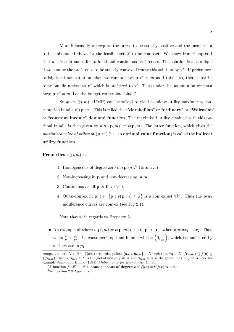
Note that with regards to Property 2,
• An example of where v(p0,m) = v(p,m) despite p0 > p is when u = ax1+ bx2. Then
when ab < p1
p2, the consumer’s optimal bundle will be
³0, mp2
´, which is unaffected by
an increase in p1.
compact subset X ⊂ <n. Then there exist points {xmin,xmax} ∈ X such that ∀x ∈ X, f(xmin) ≤ f(x) ≤f(xmax); that is, xmin ∈ X is the global min of f in X and xmax ∈ X is the global max of f in X. See forexample Simon and Blume (1994), Mathematics for Economists, Ch 30.
3A function f : <n+ → < is homogeneous of degree k if f(tx) = tkf(x) ∀t > 0.4See Section 2.9 Appendix.

9
p2 v(p,m) ≤ k lower contour set higher utility v(p,m) = k p1
Figure 2.1: Price Indifference Curves
• If preferences satisfy the local non-satiation assumption, then v(p,m) will be strictly
increasing in m. This gives a one-to-one relationship between v(p,m) and m for given
prices p. Then we can invert the function and solve for m as a function of the level of
utility, i.e. the minimal amount of income necessary to achieve utility u at prices p.
This inverse of the indirect utility function is the expenditure function investigated
in Section 2.2.
Remark 2.1 Given (p,m), the optimal bundle is chosen such that the MRS of the goods
equals the relative prices.
Proof. Intuitive. Or more technically, by solving the Lagrangian optimisation,
maxx≥0,λ
L = u(x)− λ(p.x−m) (2.1)
the first-order conditions are
∂u(x∗)
∂xi− λpi = 0 for i = 1, ..., k
Then it follows that∂u(x∗)/∂xi∂u(x∗)/∂xj
=pipj
for i, j = 1, ..., k
10
Proposition 2.2 (Roy’s Identity) For pÀ 0 and m > 0,
xi(p,m) = −∂v(p,m)/∂pi∂v(p,m)/∂m
, ∀i = 1, ..., k
Proof. Apply Envelope Theorem5 to (2.1) at x∗, i.e. u(x∗) ≡ v(p,m),
∂v(p,m)
∂pi=
∂L(x, λ)
∂pi
¯̄̄̄x(p,m) constant
= −λxi(p,m)
∂v(p,m)
∂m=
∂L(x, λ)
∂m
¯̄̄̄x(p,m) constant
= λ
Thus the ratio of the two gives xi(p,m).
2.2 Expenditure Minimisation Problem
We can look at the same problem in a different way. Suppose instead of having
(p,m) given and finding the optimal consumption bundle, we are given (p, U) i.e. the price
vector and the minimum utility level that we want attained. Then we can find the minimum
cost required to attain this,
minx≥0
p.x such that u(x) ≥ U (EMP)
Provided that the level of utility U is achievable, this problem too has a solution. And once
again if the preferences are strictly convex, the solution is unique. This optimal consumption
bundle, this time denoted h∗(p, U), is called the “Hicksian” or “compensated” demand
function. The minimum cost required to attain U is calculated by p.h∗(p, U) ≡ e(p, U) is
again an optimal value function, and is called the expenditure function.
Properties e(p, U) is,
1. Homogeneous of degree one in p, i.e. h∗(p, U) is h.g.d.0 in p. (Intuitive)
2. Non-decreasing in p (why not strictly increasing? ) and strictly increasing in U .
3. Continuous at all pÀ 0.
4. Concave in p.
5See Section 2.9 Appendix.

11
Proof of Property 4. We need to prove that e(p00, U) ≥ te(p, U)+(1−t)e(p0, U)
for 0 ≤ t ≤ 1, where p00 = tp + (1 − t)p0. As h∗(p, U) and h∗(p0, U) are the expenditure
minimising bundles at prices p and p0 respectively, we have,
p.h∗(p00, U) ≥ p.h∗(p, U)
p0.h∗(p00, U) ≥ p0.h∗(p0, U)
Multiply the former by t and the latter by 1− t, and then summing up we get,
tp.h∗(p00, U) + (1− t)p0.h∗(p00, U) ≥ te(p, U) + (1− t)e(p0, U)
But the left-hand side is {tp + (1 − t)p0}.h∗(p00, U) = p00.h∗(p00, U) = e(p00, U). Thus the
concavity is proved.
The intuition here is that as p doubles, by retaining the same consumption bundle
the expenditure will double; however one can possibly do better by choosing a more ap-
propriate consumption bundle at the new p. Thus the expenditure may increase less than
linearly.
Proposition 2.3 (Shephard’s Lemma) For pÀ 0,
hi(p, U) =∂e(p, U)
∂pi, ∀i = 1, ..., k
Proof. The Lagrangian optimisation for the EMP is,
minh≥0,λ
L = p.h+ λ(U − u(h)) (2.2)
Applying Envelope Theorem to (2.2) at h∗, i.e. p.h∗ ≡ e(p, U),
∂e(p, U)
∂pi=
∂L(h, λ)
∂pi
¯̄̄̄h(p,U) constant
= hi(p,m)

12
2.3 Duality Theory
Assuming unique solutions to the UMP and EMP, x(p,m) and h(p, U) are continu-
ously differentiable, and v(p,m) and e(p, U) are twice differentiable, the following identities
are true, demonstrating the duality property of UMP and EMP,
1. e(p, v(p,m)) ≡ m, i.e. the minimum expenditure necessary to reach utility v(p,m),
which is in turn the maximum utility attained at p and m, is m.
2. v(p, e(p, U)) ≡ U , i.e. the maximum utility from income e(p, U) is U .
3. xi(p,m) ≡ hi(p, v(p,m)), the Marshallian demand at income m is the same as the
Hicksian demand at utility v(p,m).
4. hi(p, U) ≡ xi(p, e(p, U)), the Hicksian demand at utility U is the same as the Mar-
shallian demand at income e(p, U).
2.4 Slutsky Decomposition
Proposition 2.4 The Slutsky equation is given by,
∂xj(p,m)
∂pi=
∂hj(p, U)
∂pi− ∂xj(p,m)
∂mxi(p,m) (2.3)
Proof. Use identity 4 for good j and differentiate both sides by pi,
∂hj(p, U)
∂pi=
∂xj(p,m)
∂pi+
∂xj(p,m)
∂m
∂e(p, U)
∂pi
But by Shephard’s Lemma ∂e(p,U)∂pi
= hi(p, U), which at the optimal point equals xi(p,m).
Substitution and rearranging yields (2.3).
This is another result of the Duality Theory. This holds as the optimal outcome of
the UMP is the same as that of the EMP. Note that as both the UMP and the EMP assume
given p, and hence constant m, the Slutsky equation above only holds for constant m (i.e.
not m = p.w, where w is an endowment vector). For an example of Slutsky decomposition
with price-dependent income, see Section 2.7.

13
The Slutsky equation permits an intuitive interpretation. Effectively, it allows
a notional decomposition of the effect of a change in price on Marshallian demand. An
increase in the price of any commodity, say in pi, has two effects. One, it changes the
relative price between various commodities, and two, it decreases the overall level of real
income for any consumer who purchases a positive quantity of the ith commodity. The first
leads to the substitution effect keeping the utility constant (represented by the first term
in (2.3)), and the second leads to the income effect (captured by the second term). The
minus sign for the income effect reflects the decrease in real wealth as the price increases.
Now consider the matrix of substitution terms ∂hj∂pi. This is symmetric since, using
Shephard’s Lemma again,
∂hj∂pi
=∂2e
∂pi∂pj=
∂2e
∂pj∂pi=
∂hi∂pj
The matrix is in fact negative semi-definite6 due to the concavity of the expenditure func-
tion.7 This implies that the compensated own-price effect is non-positive, i.e.
∂hi∂pi
=∂2e
∂p2i≤ 0
since negative semi-definite matrices have non-positive diagonal terms. These are properties
of “unobservable” Hicksian demands. However by using Slutsky equation we can state
that the matrixh∂xj∂pi
+∂xj∂mxi
iis also symmetric and negative semi-definite. This is now a
testable prediction. This seemingly arbitrary matrix in fact becomes useful in considering
the integrability problem. This is to say that given observed demand functions, can we
find the original utility function or the expenditure function (i.e. reversing the Roy’s Identity
or Shepherd’s Lemma)? Or more fundamentally how do we even know if a solution exists?
It turns out that the integrability condition that ensures the existence of an expenditure6A square matrix A is (see Varian Ch 26.2)
1. Positive definite if xtAx > 0 ∀x 6= 0;2. Negative definite if xtAx < 0 ∀x 6= 0;3. Positive semi-definite if xtAx ≥ 0 ∀x;4. Negative semi-definite if xtAx ≤ 0 ∀x.
7See p.55 Theorem 1.15 of Jehle and Reny 2nd ed.

14
p2
total effect = substitution effect + income effect
p1
substitution effect
Figure 2.2: Substitution and Income Effects
function that is consistent with the observed demand functions, is that this substitution
matrix is symmetric and negative semi-definite. (See Varian Ch 8.5 if interested.)
The Slutsky equation is also useful in determining the relationship between differ-
ent kind of goods. We know that the own-price substitution effect ∂hi∂pi
is non-positive. Then
for a normal good (i.e. ∂xi∂m > 0), ∂xi
∂pi< 0 unambiguously, and hence it is an ordinary
good. On the other hand for an inferior good (i.e. ∂xi∂m < 0), the sign of ∂xi
∂piis now
ambiguous. However to have ∂xi∂pi
> 0 (i.e. a Giffen good) ∂xi∂m must be negative, and hence
a Giffen good must be an inferior good.8
2.5 Welfare Measurement
Question: What is the point of Duality Theory?
Answer: For welfare analysis. For welfare measurements such as compensating and equiv-
alent variations (see below) an estimation of e(p, U) is required, but this is (and in
general EMP is) unobserved. However UMP is, and using identity 4 above, one can es-
timate the “unobservable” Hicksian demand from “observable” Marshallian demands.8Somewhat relating to this, note that for a necessary good 0 ≤ ∂xi
∂m< xi
m, i.e. the marginal increase
as one’s income increases is less than the average consumption (thus spends the extra income on somethingelse), while for a luxury good xi
m ≤ ∂xi∂m .

15
2.5.1 Money Metric Utility Functions
Consider a situation where a consumer has a choice between receiving a goods
bundle x or some income m. Given current prices p, the question is how much income,
which we will write m(p,x), would he need to be indifferent between the two. The answer
is the minimum cost required to buy a bundle z that is on the same indifference curve as
x. Thus this is the exactly the same as the EMP above with the minimum utility level U
given by u(x), and therefore the solution is
m(p,x) ≡ e(p, u(x))
This basically gives a monetary value to the utility of holding x, and is thus called the
money metric utility function.
Alternatively one could ask a question how much income μ(p;q,m) one would
need at prices p, to be as well off as having income m at prices q. It is not too difficult to
see that the solution is given by
μ(p;q,m) ≡ e(p, v(q,m))
This is called the money metric indirect utility function.
2.5.2 Compensating and Equivalent Variations
What the policy makers are interested is the welfare changes due to policy changes.
For this some measures of welfare change from (p0,m0) to (p1,m1) are required. One way
of doing this is to use compensating variation and equivalent variation which are
defined by,
v(p1,m1 − CV ) = v(p0,m0)
v(p0,m0 +EV ) = v(p1,m1)

16
http://news.bbc.co.uk/1/hi/uk/505864.stm Friday, 5 November, 1999, 17:09 GMT Can't buy me love?
Marriage can bring you as much joy as £60,000 a year, claim economists using a mathematical formula which takes into account income, personal traits and happiness levels.
It's a Sunday morning, and you are just surfacing from sleep. You turn over in bed, and put your arm around your loving, faithful partner. Life is good.
Rewind.
It's a Sunday morning, and you are just surfacing from sleep. You turn over in bed, and put your arm around your pile of £50 notes. There are 1,200 of them.
Life - apparently - is just as good.
A study by two economists claims to have found that, contrary to generations of wisdom, money can actually make you happy.
A lasting marriage brings as much happiness as having an extra £60,000 added to your pay packet, Professor Andrew Oswald of the University of Warwick and David Blanchflower of Dartmouth College in the US say.
Similarly, losing a job causes £40,000-worth of unhappiness.
The study of 100,000 people randomly sampled across the UK and US also compared satisfaction and mental well-being rates in other countries. It found there had been a decline in the number of people married (72% in the early 1970s, 55% by the late 90s). But married people said they were much happier than the unmarrieds.
Getting divorced, separated, or widowed made people much more unhappy than losing their jobs.
The happiest people were women, the highly educated, married couples, and those whose parents have not divorced, the report says. Women who co-habit are happier than those who live alone, but are not as happy as those who are married.
Happiness and satisfaction with life tend to be shaped like a U or J, it says, with high levels in youth and old age, but a drop in the 30s.
Andrew Oswald: Happily married, but not a non-financial millionaire
Note the signs assume that one is always better off in the after-change state. For example
then if a change in agricultural policy leads to a fall in price and incomes for the farmers,
the amount of compensation required can be estimated using CV at new prices. On the
other hand checking which of the possible policies make the consumers better-off can be
better analysed using EV at current prices. These estimations can be done by inverting
above definitions,
CV = e(p1, v(p1,m1))− e(p1, v(p0,m0)) = m1 − e(p1, v(p0,m0))
EV = e(p0, v(p1,m1))− e(p0, v(p0,m0)) = e(p0, v(p1,m1))−m0
2.5.3 Consumer Surplus as an Approximation
The classic tool for measuring welfare change isMarshallian consumer surplus.
If x(p) is the demand for some good as a function of its price, then the CS associated with

17
a price movement from p0 to p1 is,
CS =
Z p1
p0x(p)dp
This was first proposed by Marshall9 who used the area to the left of the market demand
curve as a welfare measure in the special case where wealth effects are absent. Let us
investigate this a little further.
Consider the case where m0 = m1 = m, and assume also that only the price of
good 1 changes from p0 to p1. Then using Shephard’s Lemma the two above variations can
be written as,
CV = m− e(p1, u0) = e(p0, u0)− e(p1, u0) =
Z p0
p1h(p, u0)dp
EV = e(p0, u1)−m = e(p0, u1)− e(p1, u1) =
Z p0
p1h(p, u1)dp
where ui = v(pi,m) for i ∈ {0, 1}. Thus the CV is the integral of the Hicksian demand
curve associated with the initial level of utility, and the EV is that associated with the final
level of utility. Hence the correct measure of welfare is an integral of the Hicksian demand
curve rather than the Marshallian. However Marshallian consumer surplus can still be used
as an approximation. We know from the Slutsky equation for own-price change that
∂hi(p, U)
∂pi=
∂xi(p,m)
∂pi+
∂xi(p,m)
∂mxi(p,m)
Thus if the good in question is a normal good (i.e. ∂xi∂m > 0), the slope of the Hicksian
demand curve ∂hi∂pi
will be less negative than that of the Marshallian demand curve ∂xi∂pi.
This implies that as shown in Figure 2.3, the Hicksian inverse demand curve ∂pi∂hi
will be
steeper than the Marshallian inverse demand curve ∂pi∂xi. It follows then that the areas to
the left of the Hicksian demand curves will bound the area to the left of the Marshallian
demand curve, and that for this normal good case,
EV > CS > CV
The relationship reverses for an inferior good. Finally in the case of a quasilinear utility
function where there is no income effect for good 1, we have h(p, u0) = x(p,m) = h(p, u1)
9Marshall, A. (1920), Principles of Economics, London: Macmillan

18
p h(p,u1) Consumer surplus p0 p1 x(p,m) h(p,u0) x
Figure 2.3: Bounds on Consumer Surplus
and hence
EV = CS = CV
In this case then the CS is an exact measure of welfare change.
2.6 Aggregation Issue
Given H consumers with income m = (m1, ...,mH), and the price vector p for
the k consumption goods, we can now calculate the individual demands xh(p,mh) =
(xh1(p,mh), ..., xhk(p,m
h)) for h = 1, ...,H. Then we can define the aggregate demand func-
tion by
X(p,m) =HXh=1
xh(p,mh)
The question is, do any of the properties described above for individual workers, such as
Roy’s Identity or Slutsky’s equation, carry through this aggregation? If that is the case then
the aggregate behaviour can be treated as it were generated by a single “representative”
consumer. It turns out though that unfortunately, the aggregate demand function will in
general possess no interesting properties other than homogeneity and continuity. This has
the implications that there is a problem for having micro underpinning on macro aggregate
theories, and also that it is hard to test consumer theories.

19
For example consider Roy’s Identity. In aggregate form what we would like is,
Xi(p,m) = −∂V/∂pi∂V/∂M
, ∀i = 1, ..., k
where V (p,m) =HPh=1
vh(p,mh) andM =HPh=1
mh. However when substituting these we get,
Xi(p,m) = −
HPh=1
∂vh/∂pi
HPh=1
∂vh/∂M
6= −HXh=1
∂vh/∂pi∂vh/∂mh
=HXh=1
xhi (p,mh)
clearly implying that Roy’s Identity does not survive aggregation in general.
Fortunately there is a necessary and sufficient condition for successful aggregation,
which is that all individual indirect utility function is of the Gorman form,
vh(p,mh) = ah(p) + b(p)mh
Then
V (p,M) =HXh=1
ah(p) + b(p)M
Try Roy’s Identity again then,
− ∂V/∂pi∂V/∂M
= −
HPh=1
∂a∂pi+ ∂b
∂piM
b(p)= −
HXh=1
∂a∂pi+ ∂b
∂pimh
b(p)= −
HXh=1
∂vh/∂pi∂vh/∂mh
and hence Xi(p,m) =HPh=1
xhi (p,mh) as desired. The point is that as can be seen from
the consumers’ demands xhi (p,mh) = 1
b(p)∂a∂pi
+ 1b(p)
∂b∂pi
mh, all consumers have the same
marginal propensity to consume good i, ∂xhi (p,mh)
∂mh = 1b(p)
∂b∂pi, which is also independent of
mh. Hence the aggregate demand function is independent of the distribution of income
but only the total income matters. Two examples of Gorman form utility functions are
quasilinear, i.e. v(p,m) = v(p)+m, and homothetic, i.e. v(p,m) = v(p)m (see Section 2.9
Appendix).

20
2.7 Application: Neoclassical Model of Labour Supply
Suppose consumption is financed out of two incomes: a labour income from H
hours worked at wage rate w, and a fixed non-labour income y. Total income is thus
m = y + wH, so that the budget constraint is now p.x = y + wH. Workers of course have
an upper limit on how many hours they can work, and this is denoted by L, i.e. 0 ≤ H ≤ L.
Now l ≡ L − H can be thought of as the total leisure time, consumed at price
w. The vector x = (x1, x2, ..., xk) on the other hand refers to consumption of goods other
than leisure, at prices p. Noting that the worker’s endowment income is now y + wL, his
optimisation problem is,
maxl,x
u(l,x) subject to wl + p.x = y + wL and 0 ≤ l ≤ L
The solution is the Marshallian demand functions l∗(w,p, y+wL) and x∗(w,p, y+wL). A
dual EMP at utility level U leads to Hicksian solutions h∗l (w,p, U) and h∗(w,p, U).
Consider then the Slutsky equations for consumption of leisure. When the price
pi of a consumption good i increases,
∂l∗
∂pi=
∂h∗l∂pi− ∂l∗
∂mxi
This is as before as the endowment income y + wL is independent of p. The endowment
income is, however, dependent on the price of leisure w: an increase in w increases the
worker’s income. Hence for l∗(w,p, y + wL) with m = y +wL,
∂l∗
∂w=
∂l∗
∂w
¯̄̄̄m constant
+∂l∗
∂m
∂m
∂w
=
µ∂h∗l∂w− ∂l∗
∂ml
¶+
∂l∗
∂mL
=∂h∗l∂w
+∂l∗
∂mH
This means that the effect of a rise in the wage on the amount of leisure taken is a sum of
a negative term (∂h∗l
∂w ) and a positive term ( ∂l∗
∂mH), assuming that leisure is a normal good.
Thus the total effect is now ambiguous. This is because on one hand a rise in the wage
rate makes leisure more expensive (lost opportunity cost of earning an income), while on
the other hand an increase in one’s income may increase the demand for leisure. This can
lead to a backward-bending labour supply curve.

21
2.8 Example
Consider the UMP
maxx1,x2
u(x1, x2) =√x1x2 subject to p1x1 + p2x2 ≤ m
Form the Lagrangian (knowing that the budget constraint will bind),
maxx1,x2,λ
L(x1, x2, λ) = x121 x
122 − λ(p1x1 + p2x2 −m)
The FOCs are
L1 =1
2x∗− 1
21 x
∗ 122 − λp1 = 0
L2 =1
2x∗ 121 x
∗− 12
2 − λp2 = 0
Lλ = −p1x∗1 − p2x∗2 +m = 0
We know that for Cobb-Douglas function with a linear constraint, the SOC is satisfied.
Now these lead to the Marshallian demands
(x∗1, x∗2) =
µ1
2
m
p1,1
2
m
p2
¶Then the indirect utility function is therefore,
v(p1, p2,m) =
µ1
2
m
p1
¶12µ1
2
m
p2
¶12
=1
2
m√p1p2
Check Roy’s Identity:
−∂v∂p1∂v∂m
= −−14mp
− 32
1 p−12
2
12p−12
1 p− 12
2
=1
2
m
p1= x∗1
Now try EMP,
minh1,h2
p1h1 + p2h2 subject toph1h2 ≥ U
The Lagrangian is this time,
minh1,h2,λ
L(h1, h2, λ) = p1h1 + p2h2 + λ(U − h121 h
122 )

22
The FOCs are
L1 = p1 − λ1
2h∗− 1
21 h
∗ 122 = 0
L2 = p2 − λ1
2h∗ 121 h
∗− 12
2 = 0
Lλ = U − h∗ 121 h
∗ 122 = 0
Which lead to the Hicksian demands
(h∗1, h∗2) =
µU
rp2p1, U
rp1p2
¶Then the expenditure function is
e(p1, p2, U) = p1U
rp2p1+ p2U
rp1p2= 2U
√p1p2
Check Shephard’s Lemma:∂e
∂p1= U
rp2p1= h∗1
We can further check the Duality identities,
m ≡ e(p1, p2, v(p1, p2,m)) = 2v(p1, p2,m)√p1p2 ⇔ v(p1, p2,m) =
1
2
m√p1p2
U ≡ v(p1, p2, e(p1, p2, U)) =1
2
e(p1, p2, U)√p1p2
⇔ e(p1, p2, U) = 2U√p1p2
x∗1 ≡ h∗1(p1, p2, v(p1, p2,m)) =1
2
m√p1p2
rp2p1=1
2
m
p1
h∗1 ≡ x∗1(p1, p2, e(p1, p2, U)) =1
2
2U√p1p2
p1= U
rp2p1
Now check Slutsky’s equation. For own-price effect on demand,
∂x∗1∂p1
= −12
m
p21∂h∗1∂p1
= −12p− 32
1 p122 U = −
1
2p−32
1 p122 ×
1
2
m√p1p2
= −14
m
p21∂x∗1∂m
x∗1 =1
2
1
p1× 12
m
p1=1
4
m
p21

23
Thus∂h∗1∂p1− ∂x∗1
∂mx∗1 = −
1
4
m
p2− 14
m
p21= −1
2
m
p21=
∂x∗1∂p1
For cross-price effect on demand,
∂x∗1∂p2
= 0
∂h∗1∂p2
=1
2p− 12
1 p− 12
2 U =1
2p− 12
1 p− 12
2 × 12
m√p1p2
=1
4
m
p1p2∂x∗1∂m
x∗2 =1
2
1
p1× 12
m
p2=1
4
m
p1p2
Thus∂h∗1∂p2− ∂x∗1
∂mx∗2 =
1
4
m
p1p2− 14
m
p1p2= 0 =
∂x∗1∂p2

24
2.9 Appendix
2.9.1 Quasi-Concavity and Quasi-Convexity
We will demonstrate the usefulness of the concepts of quasi-concavity and quasi-
convexity using Cobb-Douglas utility functions. We saw in Chapter 1 that rational and
continuous preference orderings can be represented by an ordinal utility function u(x).
This means that any positive monotonic transformation of u(x) will represent the same
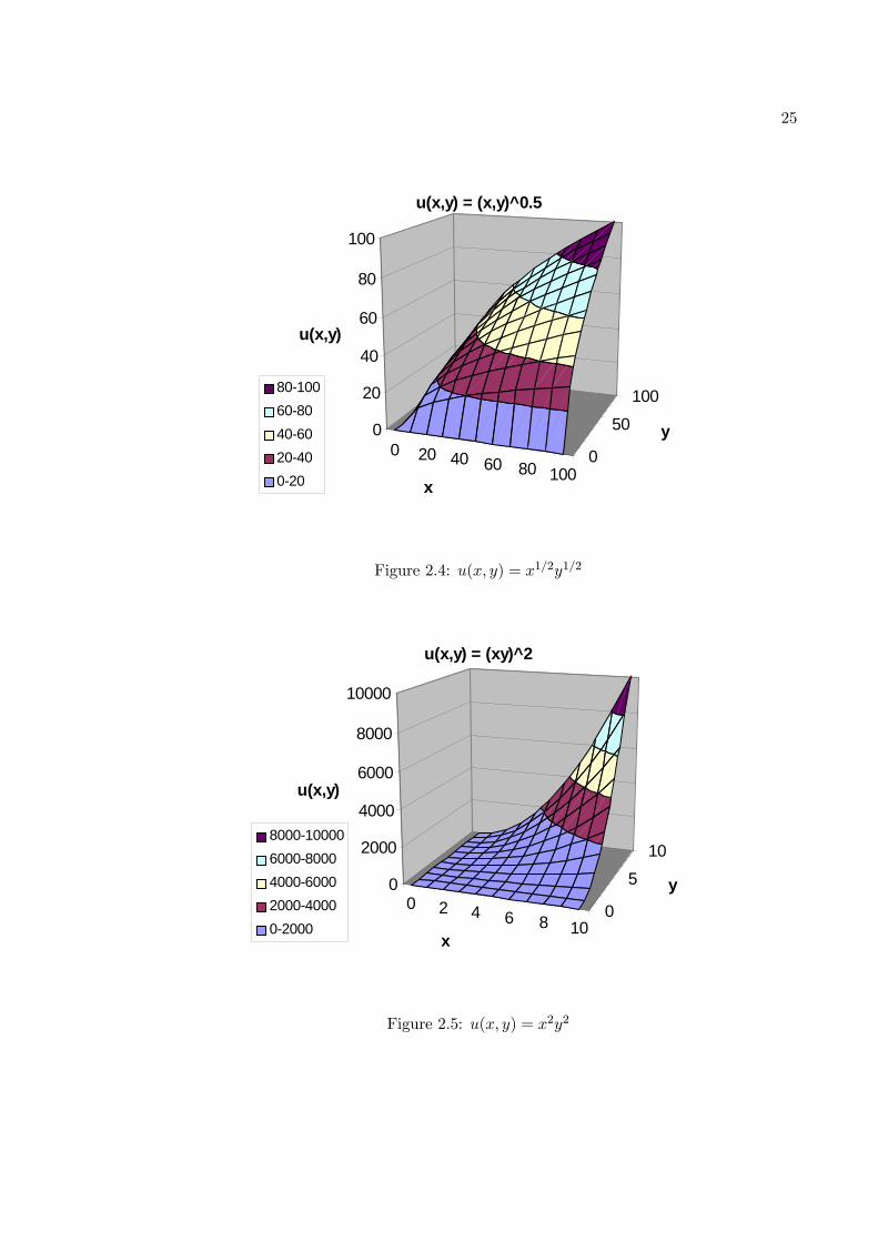
preference orderings. So consider a Cobb-Douglas utility function u(x, y) = x1/2y1/2. This
is a nice concave function on the non-negative quadrant, as shown in Figure 2.4. Now
consider the monotonic transformation g(u) = u4. The new utility function u(x, y) = x2y2
still represents the original preference orderings, but now is no longer concave (though not
convex either), as seen in Figure 2.5. What this is demonstrating is that concavity and
convexity of a function are cardinal and not ordinal properties. This is where properties of
quasi-concavity and quasi-convexity come in useful:
Definition 2.1 A function f defined on a convex subset X ⊂ <n is quasi-concave if
∀a ∈ < the upper level set
C+a ≡ {x ∈ X : f(x) ≥ a}
is a convex set. Similarly, f is quasi-convex if ∀a ∈ < the lower level set
C−a ≡ {x ∈ X : f(x) ≤ a}
is a convex set.
In our Cobb-Douglas examples the upper level sets are basically the sets of (x, y)
such that u(x, y) is greater than equal to a certain utility level, i.e. the upper contour set
of the indifference curves. As can be seen from Figures 2.4 and 2.5 that these upper level
sets are convex in both cases, i.e. the quasi-concavity property is preserved by a positive
monotonic transformation. Thus unlike concavity and convexity, quasi-concavity and quasi-
convexity are ordinal properties. Note that it is easily seen that if f(x) is concave then it
is also quasi-concave, and similarly convexity implies quasi-convexity.
25
0 20 40 60 80 1000
50
100
0
20
40
60
80
100
u(x,y)
x
y
u(x,y) = (x,y)^0.5
80-10060-8040-6020-400-20
Figure 2.4: u(x, y) = x1/2y1/2
0 2 4 6 8 100
5
10
0
2000
4000
6000
8000
10000
u(x,y)
x
y
u(x,y) = (xy)^2
8000-100006000-80004000-60002000-40000-2000
Figure 2.5: u(x, y) = x2y2

26
2.9.2 Envelope Theorem
Theorem 2.1 (Envelope Theorem for Unconstrained Optimisation) Consider the
unconstrained maximisation problem of a function u = f(x, y;φ) with respect to variables
(x, y) at a parameter value φ,
maxx,y
u = f(x, y;φ)
Given the solution (x∗, y∗) at φ, let v(φ) = f(x∗(φ), y∗(φ);φ) denote the maximum-value
function. Thendv(φ)
dφ=
∂f
∂φ
i.e. (x, y) can be treated as constants when differentiating the maximum-value function with
respect to φ.
Proof. First note that the first-order conditions of the maximisation problem are,
∂f
∂x=
∂f
∂y= 0
Now totally differentiate f(x, y;φ) with respect to the parameter φ at the optimal point
(x∗(φ), y∗(φ)),dv(φ)
dφ=
∂f
∂x
∂x∗(φ)
∂φ+
∂f
∂y
∂y∗(φ)
∂φ+
∂f
∂φ
But the first two terms disappear using the first-order conditions.
Theorem 2.2 (Envelope Theorem for Constrained Optimisation) Consider the con-
strained maximisation problem of a function u = f(x, y;φ) with respect to variables (x, y)
at a parameter value φ,
maxx,y
u = f(x, y;φ) subject to g(x, y;φ) = 0
Given the solution (x∗, y∗) at φ, let v(φ) = f(x∗(φ), y∗(φ);φ) denote the maximum-value
function. Thendv(φ)
dφ=
∂L
∂φ
where L(x, y, λ;φ) is the Lagrangian function of the problem with the multiplier λ.

27
Proof. First consider the Lagrangian optimisation,
maxx,y,λ
L = f(x, y;φ)− λg(x, y;φ)
The first-order conditions are,
Lx =∂f
∂x− λ
∂g
∂x= 0
Ly =∂f
∂y− λ
∂g
∂y= 0
Lλ = −g(x∗, y∗;φ) = 0
Now totally differentiate f(x, y;φ) with respect to the parameter φ at the optimal point
(x∗(φ), y∗(φ)),dv(φ)
dφ=
∂f
∂x
∂x∗(φ)
∂φ+
∂f
∂y
∂y∗(φ)
∂φ+
∂f
∂φ
Using the first two first-order conditions this becomes,
dv(φ)
dφ= λ
∂g
∂x
∂x∗(φ)
∂φ+ λ
∂g
∂y
∂y∗(φ)
∂φ+
∂f
∂φ
But differentiating the third first-order condition yields
∂g
∂x
∂x∗(φ)
∂φ+
∂g
∂y
∂y∗(φ)
∂φ+
∂g
∂φ= 0
Substituting this back we get
dv(φ)
dφ=
∂f
∂φ− λ
∂g
∂φ=
∂L
∂φ
keeping (x, y) constant.
2.9.3 Quasilinear Utility Function
A quasilinear utility function has the following form,
U(x0, x1, ..., xk) = x0 + u(x1, ..., xk)
i.e. it is linear in one or more (in this case good 0) of the goods. Investigate this for a
two-good case:
maxx0,x1
U(x0, x1) = x0 + u(x1) subject to x0 + p1x1 ≤ m

28
where p0 is normalised to 1. By substitution U(x0, x1) = u(x1) + m − p1x1, which has
the first-order condition u0(x1) = p1. This is independent of m; i.e. given relative prices
the consumer will consume the same amount of x1 no matter how much his income is. An
example may be one’s demand for pencils: how much would your demand change as your
income changes? It is most likely that any increases in income would go into consumption
of other goods. Diagrammatically this implies that the indifference curves are parallel in
the direction of x0, i.e. the distances between any two indifference curves are the same at
all points of the curves.
Note that, as in the first-order condition the demand of good 1 is only a function
of the price of good 1, we can write the demand function as x1(p1). The demand for good
0 is then x0 = m − p1x1(p1) from the budget constraint. Substituting this back into the
utility function then yields the indirect utility function
V (p1,m) = m− p1x1(p1) + u(x1(p1)) = v(p1) +m
where v(p1) = u(x1(p1))− p1x1(p1).
2.9.4 Homogeneous and Homothetic Utility Functions
Definition 2.2 A function u(x) is said to be homogeneous of degree k if
u(tx) = tku(x) ∀t > 0
Homogeneous functions have many useful properties. Consider the two input case:
Properties If u(x1, x2) is a once differentiable homogeneous function (i.e. of any degree
k),
1. The partial derivatives u1 and u2 are homogeneous of degree k − 1.
2. The slope of the tangent line to the level sets (i.e. the slope of the indifference
curve if u(x) is a utility function) is constant along each ray from the origin.
3. (Euler’s Theorem) For all (x1, x2),
x1∂u
∂x1(x) + x2
∂u
∂x2(x) = ku(x)

29
For proofs see Simon and Blume Ch 20.1. Property 2 implies that if u(x) is a
utility function, then the MRS is constant along rays from the origin, and that the income
elasticity of demand is identically 1.
One problem is though that homogeneity is not an ordinal property. For exam-
ple u(x1, x2) = x1x2 is clearly a homogeneous function, but even the simplest monotonic
transformation g(u(x)) = u(x) + 1 makes the resulting function v(x1, x2) = x1x2 + 1 non-
homogeneous. Instead we can define another set of functions,
Definition 2.3 A function v(x) is said to be homothetic if it is a monotone transforma-
tion of a homogeneous function, that is, if there is a monotonic transformation g(z) and a
homogeneous function u(x) such that v(x) = g(u(x)) ∀x in the domain.
Clearly then a monotonic transformation of a homothetic function is homothetic,
and hence the property is now ordinal. As we also know that the MRS is an ordinal concept
(note marginal utility is not), homothetic functions also have property that the slopes of
the indifference curves are constant along each ray from the origin. In fact the converse is
also true, i.e. if the slopes of the indifference curves are constant along each ray from the
origin, then the function is homothetic (but not necessarily homogeneous). Thus we have
another definition for homothetic functions,
Definition 2.4 A utility function v(x) is homothetic if the MRS is homogeneous of degree
zero.
Now if the MRS is constant no matter what the income level is, it implies that
the consumer will spend the same proportion of his income on each goods. This means
that his demand for each good will be linear to his income (i.e. double the income, double
the demand). Moreover if we define homotheticity by restricting the homogeneity of the
underlying function u(x) to degree 1 (as Varian does), then we know that doubling con-
sumption of each good doubles the level of utility. Thus utility will also be linear to his
income. Hence one can write the indirect utility function in the form v(p,m) = v(p)m
where v(p) = v(p, 1).

30
Chapter 3
Producer Theory
Hal Varian, Microeconomic Analysis, 3rd ed. (1992), Chs 1-6
3.1 Technology
A production plan is a list of net outputs of various goods, represented by a
vector y ∈ <n where yj is negative (positive) if the jth good serves as a net input (output).
The set of all technologically feasible production plans is the firm’s production possibility
set, which is denoted by Y ∈ <n.
Sometimes production possibilities are written in a manner which seems more
intuitive, at least for plans which involve only one output and one or more inputs. In this
case the output can be written as a scaler y and the input as a vector x, with the production
plan being (y,−x). In this case we can define an input requirement set, as the set of all
input bundles that produce at least y,
V (y) =©x ∈ <n
+ : (y,−x) ∈ Yª
The isoquant Q(y) is the set of all input bundles that produce exactly y,
Q(y) =©x ∈ <n
+ : x ∈ V (y) and x /∈ V (y0) for y0 > yª
The examples of isoquants: Cobb-Douglas Q(y) =©(x1, x2) ∈ <2+ : y = xa1x
1−a2
ª; Leontief
Q(y) =©(x1, x2) ∈ <2+ : y = min[ax1, bx2]
ª.

31
3.2 Possible Restrictions on Technology Set
1. Monotonicity - {x ∈ V (y) and x0 ≥ x} implies x0 ∈ V (y), i.e. can always produce
the same amount of output by larger inputs.
2. Convexity - V (y) is a convex set, i.e. if x,x0 ∈ V (y) then tx + (1 − t)x0 ∈ V (y)
∀0 ≤ t ≤ 1. This is equivalent to saying that the associated production function is
quasi-concave, as V (y) ={x : f(x) ≥ y} which is just the upper contour set of f(x).
3. Regularity - V (y) is a closed, non-empty set ∀y ≥ 0. Non-empty set means that
there is some conceivable way of producing any given level of output.
3.3 Technical Rate of Substitution
Technical rate of substitution describes how much more of input i one must
have to maintain the same output if input j is decreased by 1. This is just the slope of the
isoquant surface. For example for two inputs, the definition of an isoquant is f(x1, x2) ≡ y
and thus,
dy =∂f
∂x1dx1 +
∂f
∂x2dx2 = 0
ordx2dx1
= −∂f/∂x1∂f/∂x2
Thus TRS is the ratio of the marginal productivities.
3.4 Returns to Scale
A technology is said to have,
1. Constant returns to scale if f(tx) = tf(x) ∀t ≥ 0.
2. Increasing returns to scale if f(tx) > tf(x) ∀t > 1.
3. Decreasing returns to scale if f(tx) < tf(x) ∀t > 1.

32
Note the difference in the restrictions on t. Note also for IRS the PPF is convex
(or PPS is concave) and thus there is no competitive producer theory for IRS production
technologies. Alternative definitions for CRS are: ∀y ∈ Y , ty ∈ Y ∀t ≥ 0, or ∀x ∈ V (y),
tx ∈ V (ty) ∀t ≥ 0.
Example (Cobb-Douglas): y = xa1xb2 ⇒ f(tx1, tx2) = (tx1)
a(tx2)b = ta+bxa1x
b2 =
ta+bf(x1, x2). So CRS when a+ b = 1, IRS when > and DRS when <.
3.5 Profit Maximisation Problem
Here we consider a competitive, or a price-taker firm. Let (y,−x) denote
a production plan, with the associated vector of output prices p and input prices w. In
general prices may depend on the production plan, so we have p(y,−x) and w(y,−x).
However if the markets are perfectly competitive, i.e. the representative firm is too small
to affect the prices of inputs or outputs through its production plans, then p(y,−x) = p
and w(y,−x) = w.
The profits for a given production plan are the difference between revenue and
cost, i.e. p.y −w.x. The profit maximisation problem is to maximise this subject to the
technological constraints, i.e. given (p,w),
maxy,x
π(y,−x) = p.y −w.x subject to (y,−x) ∈ Y (PMP)
Note that for the one-output good case the constraint becomes simply f(x) = y. Now
for an interior solution to exist, typically it is sufficient that the technology be strictly
convex, regular, and p,w > 0. The solution (y∗(p,w),−x∗(p,w)) is the output sup-
ply and factor demand functions. The optimal value function is the profit function
π(y∗(p,w),−x∗(p,w)) = π(p,w), i.e. the maximum profit that the firm can make at prices
(p,w). We now investigate the properties of these functions.
3.5.1 Demand and Supply Functions
1. Both factor demand and supply functions are homogeneous of degree 0, i.e. x∗i (tp, tw) =
x∗i (p,w), y∗j (tp, tw) = y∗j (p,w) ∀t > 0. (Intuitive)
33
2. The factor demand curve is downward-sloping, i.e. ∂xi/∂wi < 0 ∀i.
3. The change in a firm’s demand for input i when the price of input j changes equals
the change in the firm’s demand for input j when the price of input i changes, i.e.
∂xi/∂wj = ∂xj/∂wi ∀i 6= j.
Proof of Properties 2 & 3. Let us consider a one-good output, two-good
input case, with the price of the output good normalised to p = 1. Then for the production
function f(x1, x2), the first-order conditions are,
∂f(x1(w1, w2), x2(w1, w2))
∂x1≡ w1
∂f(x1(w1, w2), x2(w1, w2))
∂x2≡ w2
i.e. marginal productivity must equal marginal cost at all input prices (w1, w2). So when
(w1, w2) change (x1, x2) must change to keep these equalities, i.e.,
f11∂x1∂w1
+ f12∂x2∂w1
= 1, f21∂x1∂w1
+ f22∂x2∂w1
= 0
f11∂x1∂w2
+ f12∂x2∂w2
= 0, f21∂x1∂w2
+ f22∂x2∂w2
= 1
or in a matrix form, ⎛⎝ f11 f12
f21 f22
⎞⎠⎛⎝ ∂x1∂w1
∂x1∂w2
∂x2∂w1
∂x2∂w2
⎞⎠ =
⎛⎝ 1 0
0 1
⎞⎠The first matrix is the Hessian matrix which we know for a regular maximum (i.e. ruling
out zero second derivative) to be symmetric negative definite. Therefore it is non-singular
and can be inverted, ⎛⎝ ∂x1∂w1
∂x1∂w2
∂x2∂w1
∂x2∂w2
⎞⎠ =
⎛⎝ f11 f12
f21 f22
⎞⎠−1
The matrix on the left-hand side is the substitution matrix, i.e. it describes how the firm
substitutes one input for another as the factor prices change, which according to this result
is simply the inverse of the Hessian matrix. Now as the inverse of a symmetric negative
definite matrix is also symmetric negative definite, we have the results that the diagonal
elements ∂x1∂w1, ∂x2∂w2
< 0, and that ∂x1∂w2
= ∂x2∂w1.
34
3.5.2 Profit Function
π(p,w) possesses some important properties that follow directly from its defin-
itions (i.e. no assumptions about convexity, monotonicity or other sorts of regularity is
necessary),
1. Non-decreasing in p, non-increasing in w. Thus if p0j ≥ pj for all outputs and w0i ≤ wi
for all inputs, then π(p0,w0) ≥ π(p,w).
2. Homogeneous of degree 1 in (p,w) for (p,w)À 0, i.e. unchanged in real terms.
3. Convex in (p,w) for (p,w) > 0, i.e. if p3 = tp1+(1− t)p2 and w3 = tw1+(1− t)w2
for 0 ≤ t ≤ 1, then π(p3,w3) ≤ tπ(p1,w1) + (1− t)π(p2,w2).
Proof. By definition of profit maximisation,
p1.y1 −w1.x1 ≥ p1.y3 −w1.x3 ⇒ tp1.y1 − tw1.x1≥tp1.y3 − tw1.x3
p2.y2 −w2.x2 ≥ p2.y3 −w2.x3 ⇒ (1− t)p2.y2 − (1− t)w2.x2≥(1−t)p2.y3 − (1− t)w2.x3
Add the two,
tπ(p1,w1) + (1− t)π(p2,w2) ≥ {tp1 + (1−t)p2}y3 − {tw1 + (1−t)w2} .x3
= π(p3,w3)
i.e. always can do at least as well with a possibility of pursuing the optimal in-
put/output choices at the extreme prices. (See Fig 3.1)
4. Continuous in (p,w) when π(p,w) is well-defined and (p,w)À 0.
Now similar to Roy’s Identity in UMP, we have the following,
Proposition 3.1 (Hotelling’s Lemma) Suppose π(p,w) is differentiable in (p,w). Let
(y∗,−x∗) be the optimal production plan at that price. Then,
yj =∂π
∂pjand − xi =
∂π
∂wi∀i, j = 1, 2, ...

35
π π(p) passive profit function py* (p*) – wx* (p*) π(p*) 0 p* p
Figure 3.1: Single output good profit function
Proof. We prove this for a one-output good case using the Envelope Theorem for
unconstrained optimisation. By substitution the PMP becomes simply
maxx
π(x) = p.f(x)−w.x
for which we obtain the factor demands x∗(p,w) and the profit function π(p,w). Now to
investigate what happens to the optimal-value function π(p,w) as the parameters (p,w)
change, the Envelope Theorem states that we can treat the choice variables x∗(p,w) as
constants, and hence,
∂π
∂p= f(x∗) = y∗
∂π
∂wi= −x∗i
Intuitively this is stating that a unit increase in pj (while keeping all other prices
constant - hence the partial derivative) has two effects: a direct effect where profit increases
by yj , and an indirect effect where the firm re-chooses the optimal production plan (y∗,−x∗).
However at the optimal point for an infinitesimal change in pj the latter effect is zero, and
thus the change in profit will equal yj . A similar argument can be made for the effect of a
change in wi.
This relationship between π(p,w) and (y,−x) allows us to state, using the already
stated properties of the profit function, the following properties for the supply and factor
36
demand functions,
1. π(p,w) is homogeneous of degree 1 in (p,w) implies that output supply and factor
demand functions are h.d.0.
2. As the matrix of the second-order derivatives (the Hessian matrix) of a convex function
is positive semi-definite, and π(p,w) is a convex function in (p,w), it follows that the
matrices of price derivatives of the supply and factor demand functions are positive
semi-definite. Moreover Hotelling’s Lemma implies that this matrix is symmetric. For
example for a two-good case,⎛⎝ ∂2π∂p21
∂2π∂p2∂p1
∂2π∂p1∂p2
∂2π∂p22
⎞⎠ =
⎛⎝ ∂y1∂p1
∂y1∂p2
∂y2∂p1
∂y2∂p2
⎞⎠which is the substitution matrix. The symmetry ∂yj
∂pk∀j, k provides the strongest
prediction of PMP. The positive semi-definiteness implies that the diagonal elements
are non-negative, i.e. an increase in own price will always weakly increases y or weakly
decrease x.
3.5.3 Example
Consider a Cobb-Douglas production function y = LaKb where a + b < 1. Then
the PMP is,
maxL,K
py −wL− rK subject to y = LaKb
By substitution this is,
maxL,K
pLaKb − wL− rK
and therefore the FOCs are,
∂
∂L: apL∗a−1K∗b − w = 0
∂
∂K: bpL∗aK∗b−1 − r = 0

37
Solving this simultaneous equations yields the factor demand functions,
L∗ =
(³ aw
´1−bµb
r
¶b
p
) 11−a−b
K∗ =
(³ aw
´aµb
r
¶1−ap
) 11−a−b
Check the properties of these factor demands. First of all they should be decreasing in their
own prices,
∂L∗
∂w= −
µ1− b
1− a− b
¶L∗
w
∂K∗
∂r= −
µ1− a
1− a− b
¶K∗
r
which for a+ b < 1 are indeed negative. Secondly the cross-price effects must be equal,
∂L∗
∂r= − 1
1− a− b
(³ aw
´1−bµb
r
¶1−ap
) 11−a−b
=∂K∗
∂w
The profit-maximising output supply function is given by,
y∗ = L∗aK∗b
=
(³ aw
´aµ b
r
¶b
pa+b
) 11−a−b
Check that this is weakly increasing in its own-price,
∂y∗
∂p=
a+ b
1− a− b
y∗
p> 0
Finally the profit function is (after a lot of fiddly maths),
π(p,w, r) = py∗ − wL∗ − rK∗
= (1− a− b)
(³ aw
´aµb
r
¶b
p
) 11−a−b
Note that this is only strictly positive for a + b < 1, i.e. PMP is only feasible for DRS
production functions.

38
Now check Hotelling’s Lemma,
∂π
∂p=
(³ aw
´aµb
r
¶b
pa+b
) 11−a−b
= y∗
∂π
∂w= −
(³ aw
´1−bµb
r
¶b
p
) 11−a−b
= −L∗
∂π
∂r= −
(³ aw
´aµb
r
¶1−ap
) 11−a−b
= −K∗
as required.
3.6 Cost Minimisation Problem
The problem with PMP is that it is only applicable if (a) the firm operates com-
petitively (i.e. the firms are price-takers), and (b) the production possibility set is convex.
CMP on the other hand permits analyses of problems such as that of a natural monopoly
operating in competitive input markets, by modelling the behaviour of the firm as that of
minimising the cost of producing a given output. The firm’s optimisation problem is given
by,
minx
w.x subject to x ∈ V (y) (CMP)
Once again we will consider a one-output good case for simplicity, in which case the con-
straint is f(x) = y for a given output y. This can be used as usual by using a Lagrangian
optimisation,
minx,λ
L(x, λ) = w.x+λ(y − f(x)) (3.1)
The FOCs are
wi − λ∂f(x∗)
∂xi= 0 ∀i = 1, ..., n
f(x∗) = y
which immediately implies that
wi
wj=
∂f(x∗)/∂xi∂f(x∗)/∂xj
∀i, j = 1, ..., n

39
i.e. the technical rate of substitution equals the price ratio, or the economic rate of
substitution - at what rate two factors can be substituted at a constant cost. This,
together with the technological constraint then yields the optimal input levels x∗(w, y)
given the required output y; and hence these are called the conditional factor demand
functions.
Now the optimal value function for the CMP is the cost function c(w, y), which
is the minimum cost required to produce the given output y at prices w. c(w, y) possesses
the following properties that follow directly from its definitions,
1. Non-decreasing in w. Thus if w0 ≥ w, then c(w0, y) ≥ c(w, y).
2. Homogeneous of degree 1 in w, i.e. c(tw, y) = tc(w, y) ∀t > 0. This is stating that the
composition of the cost minimising bundle is unchanged with a scaler multiplication of
factor prices. This follows from the fact that the conditional factor demands depend
on relative prices.
3. Concave in w, i.e. c(tw1 + (1− t)w2, y) ≥ tc(w1, y) + (1− t)c(w2, y) ∀0 ≤ t ≤ 1.
Proof. By definition of cost minimisation, where w3 = tw1 + (1− t)w2,
w1.x1 ≤ w1.x3 ⇒ tw1.x1 ≤ tw1.x3
w2.x2 ≤ w2.x3 ⇒ (1− t)w2.x2 ≤ (1− t)w2.x3
Add the two,
tc(w1, y) + (1− t)c(w2, y) ≤ {tw1 + (1−t)w2} .x3
= c(w3, y)
i.e. always can do at least as well with a possibility of pursuing the optimal input
choices at the extreme prices. (See Fig 3.2)
4. Continuous in w for wÀ 0.
Proposition 3.2 (Shephard’s Lemma) Suppose c(w, y) is differentiable in prices w for
a fixed y. Let x∗ denote the optimal input vector at that price. Then,
x∗i =∂c
∂wi∀i = 1, 2, ...

40
c passive cost function wx* (w*) c(w,y) c(w*,y) 0 w* w
Figure 3.2: Single input factor cost functoin
Proof. This time we use the Envelope Theorem for constrained optimisation.
Here our Lagrangian is given by (3.1). Thus when factor price wi changes its effect on the
cost function c(w, y) is given by,
dc(w, y)
dwi=
∂L
∂wi= x∗i
Once again this relationship between c(w, y) and x allows us to state, from the
properties of the cost function, the following properties for the cost function and the con-
ditional factor demand functions,
1. c(w, y) is non-decreasing in factor prices. This follows immediately from Shephard’s
Lemma above, where x∗i (w, y) ≥ 0.
2. c(w, y) is homogeneous of degree 1 in w ⇒ x∗i (w, y) are h.d.0.
3. c(w, y) is concave inw⇒ the matrix of price derivatives of the factor demand functions⎛⎝ ∂x1∂w1
∂x1∂w2
∂x2∂w1
∂x2∂w2
⎞⎠ =
⎛⎝ ∂2c∂w21
∂2c∂w2∂w1
∂2c∂w1∂w2
∂2c∂w22
⎞⎠is symmetric negative semi-definite. It follows then that the cross-price effects are
symmetric and the own-price effects are non-positive, i.e.
∂xi∂wj
=∂xj∂wi
∀i, j and∂xi∂wi≤ 0 ∀i

41
3.6.1 Example: Cobb-Douglas Technology
Consider the CMP for the Cobb-Douglas production function y = LaKb,
minL,K
wL+ rK subject to LaKb ≥ Y
for a given output level Y . The Lagrangian is,
minL,K
£(L,K, λ) = wL+ rK + λ(Y − LaKb)
The FOCs are,
£L = w − λaY
L∗= 0
£K = r − λbY
K∗ = 0
£λ = Y − L∗aK∗b = 0
Solving for λ yields,
λ =1
kw
aa+b r
ba+bY
1−a−ba+b where k = a
aa+b b
ba+b
Substituting this back into the first two FOCs yields the factor demand functions given Y ,
L∗ =a
k
³ rw
´ ba+b
Y1
a+b
K∗ =b
k
³wr
´ aa+b
Y1
a+b
It is easy to see that these conditional demands are homogeneous of degree 0, and that the
own-price effects are non-positive. Check the symmetry in the cross-price effects:
∂L∗
∂r=
ab
(a+ b) kw−
ba+b r−
aa+bY
1a+b =
∂K∗
∂w
The cost function is then,1
c(w, r, Y ) = wL∗ + rK∗
=
µa+ b
k
¶w
aa+b r
ba+bY
1a+b
1In Varian Ch 4.3 example the cost function (for A = 1) is given as ab
ba+b + a
b
−aa+b w
aa+b r
ba+b Y
1a+b .
One can check that this expression and ours are equivalent by substituting the expression for k.

42
Again it is easy to see that this function is both non-decreasing, and homogeneous of degree
1, in (w, r). Note that the marginal cost is then,
MC(w, r, Y ) =∂c(w, r, Y )
∂Y
=1
kw
aa+b r
ba+bY
1−a−ba+b
= λ
demonstrating that the Lagrange multiplier in the CMP is simply the marginal cost.2
Check also Shephard’s Lemma,
∂c
∂w=
a
k
³wr
´− ba+b
Y1
a+b = L∗
∂c
∂r=
b
k
³wr
´ aa+b
Y1
a+b = K∗
Finally note that unlike with the PMP example, none of the above results require
any constraints on the size of a+ b. Thus all of the results are valid whether the production
function is DRS, CRS or IRS.
3.6.2 Example: Leontief Technology
The Leontief technology is given by
f(x1, x2) = min[ax1, bx2]
The isoquants are then right-angles which are not differentiable at the corner. Thus one
cannot use the normal first-order condition to find the solution. However we know that the
firm will not waste any input with a positive price, so it must operate at the corner where
y = ax1 = bx2. Hence the conditional factor demands are
(x∗1, x∗2) =
³ya,y
b
´and the cost function is given by
c(w1, w2, y) = w1y
a+w2
y
b= y
³w1a+
w2b
´2This actually follows directly from the Envelope Theorem. For our constrained optimisation, in consid-
ering changes in the parameter y,dc(w, y)
dy=
∂L
∂y= λ

43
3.6.3 Example: Linear Technology
Consider a linear technology
f(x1, x2) = ax1 + bx2
This implies that the two input goods are perfect substitutes, and the firm will use whichever
is cheaper. Hence immediately we know that the conditional factor demands are
(x∗1, x∗2) =
⎧⎪⎪⎪⎨⎪⎪⎪⎩¡ya , 0¢if w1
a < w2b¡
0, yb¢if w1
a > w2b
{(x1, x2) : ax1 + bx2 = y; x1, x2 ≥ 0} if w1a = w2
b
The cost function is then
c(w1, w2, y) = minhw1a,w2b
iy
Here it is very important to note that this problem cannot be solved using the equality
constraint Lagrangians optimisation. The solution is a corner solution as long as w1a 6= w2
b
rather than an interior solution, and thus the FOC will not be satisfied. For this then the
Kuhn-Tucker conditions are required (see Varian p.57-8).
3.7 Duality
We have seen that given any technology, it is straightforward to derive its cost
function by simply solving the CMP. The question can be raised then as to whether this
process can be reversed, i.e. given a cost function, can we “solve for” a technology that
could have generated that cost function. If this is so then the cost function will contain
essentially the same information that the production function contains. Then any concept
defined in terms of the properties of the production function has a “dual” definition in terms
of the properties of the cost function and vice versa. This is the principle of duality.
The answer to this question is “yes, provided the technology is convex and monotonic.”
To see this define a special form of the input requirement set for a given c(w, y),
V ∗(y) = {x : w.x ≥ w.x(w, y) = c(w, y) ∀w ≥ 0}

44
x2 Boundary for the original input requirement set V(y) Boundary for the convexified and monotonised set V*(y) Isocost lines for different w x1
Figure 3.3: Non-convex Input Requirement Set V (y)
i.e. all the possible input factor combinations that would produce at least y at a cost
greater than or equal to the minimised cost function c(w, y) for all factor prices w. We can
now try and relate this input requirement set, constructed from c(w, y), to the usual input
requirement set V (y) constructed from f(x). The claim is, if V (y) represents a convex and
monotonic technology, then the two are identical. This is because for a convex, monotonic
input requirement set V (y), each point on the boundary is a cost-minimising factor demand
for some price vector w ≥ 0. If the technology is non-convex or non-monotonic, V ∗(y)
will be a convexified, monotonised version of V (y). The difference V ∗(y) − V (y) is an
area that will not be a solution to a CMP and therefore contains no economically relevant
information. Thus the cost function summarises all of the economically relevant aspects of
the firm’s technology.
3.7.1 Example: Leontief Technology
Consider a Leontief technology f(x1, x2) = min[x1, x2]. We know from Section
3.6.2 that the conditional factor demands are
(x∗1, x∗2) = (y, y)
and the cost function is given by
c(w1, w2, y) = w1x1 + w2x2 = (w1 + w2) y

45
This is the minimised cost of producing y for an input price vector (w1, w2). Conversely
if we fix the cost at c(w1, w2, y), then one can draw the isocost lines for each values of
(w1, w2) for given y (i.e. inputs (x1, x2) that can produce y at that cost when input prices
are (w1, w2)),
w1x1 + w2x2 = c(w1, w2, y)⇔ x2 =c(w1, w2, y)
w2− w1
w2x1
For our Leontief technology the isocosts are then,
x2 =(w1 + w2) y
w2− w1
w2x1 =
µw1w2+ 1
¶y − w1
w2x1
Now for a given value of y, these isocosts will pass through the point (x1, x2) = (y, y) for
all values of (w1, w2) (can check by substituting x1 = x2 = y in the equation). Also at
the extremes (w1, w2) = (0, w2) and (w1, 0) the isocosts are horizontal x2 = y and vertical
lines x1 = y respectively. Hence the boundary traced out by isocosts for different values of
(w1, w2) is a right-angle shape with the corner at (y, y), which is equivalent to the production
function min[x1, x2], as predicted.
3.8 Aggregation
Define the aggregate supply of competitive producers by the aggregate production
possibility set,
Y =FXf=1
Y f =
⎧⎨⎩y ∈ <N : y =FXf=1
yf for some yf ∈ Y f
⎫⎬⎭where yf are the production plans for firm f , and y is the associated aggregated production
plan. Then,
Proposition 3.3 An aggregate production plan y maximises the aggregate profit p.y if and
only if each firm’s production plan yf maximises its individual profit p.yf .
Proof. First check the “only if” (⇒) by contradiction. Suppose that y =PF
f=1 yf
maximises aggregate profit but some firm k could have higher profits by choosing y0k. Then

46
aggregate profits could be higher by choosing plan y0k for firm k and the same {yf} for
firms f 6= k which contradicts the fact that y is the maximising production plan.
Next check the “if” (⇐). Let {yf} for firms f = 1, ..., F be a set of profit-
maximising production plans for the individual firms. Suppose that y =PF
f=1 yf is not
profit-maximising at prices p. This means that there is some other production plan y0 =PFf=1 y
0f with y0f ∈ Y f that has higher aggregate profits,
p.FXf=1
y0f > p.FXf=1
yf ⇔FXf=1
p.y0f >FXf=1
p.yf
But for the right-hand side inequality to be valid there must be at least one firm for whom
p.y0f > p.yf . This is again a contradiction.
This implies then that, unlike Consumer Theory, for Producer Theory the predic-
tions of the theory carries through to the aggregate level.

47
Chapter 4
Monopoly
Varian Ch14
Mas-Colell, Whinston and Green Ch 12.B
4.1 Monopoly Profit Maximisation
A monopoly is a price-maker, as opposed to a competitive firm who is a price-
taker. This is because a monopoly firm can now affect the output good price by varying
its output level. Thus its maximisation problem is now,
maxy
π(y) = p(y)y − c(y)
where p(y) is the inverse demand function. The FOC is then
p(y) + p0(y)y = c0(y) (4.1)
i.e. the optimal output level is where the marginal revenue of an increase in output equals
its marginal cost. Here unlike with a competitive firm, the marginal revenue now includes
the effect of a drop in the price due to the increased output. Now this can be rewritten as,
p(y)
½1− 1
(y)
¾= c0(y)
where (y) = −pydydp is the price elasticity of demand facing the monopolist. It follows
then that at the optimal level of output, the elasticity of demand must be greater than 1,
as otherwise the marginal revenue will be a negative value.

48
4.1.1 Example: Linear Demand
Consider a downward-sloping linear demand function for a monopoly
y(p) =a
b− 1
bp where a, b > 0
The marginal revenue line is then twice as steep as the indirect demand,
p(y) = a− by
MR = a− 2by
The price elasticity of demand is:
−py
dy
dp= −
µa− by
y
¶µ−1b
¶=
a
by− 1
This is decreasing in y, and the unit elasticity occurs at y = a2b . Hence the optimal output
level for the monopoly will be less than a2b . (Can you show this diagrammatically? )
4.2 Monopoly Inefficiency
We can see immediately from (4.1) that p(ym) > c0(ym), i.e. under monopoly price
exceeds marginal cost. Thus the monopoly output is inefficient. To investigate this further,
assume for simplicity that the market demand curve x(p) is generated by maximising the
utility of a single representative consumer with a quasilinear utility function,
U(x, y) = u(x) + y
The y-good is a proxy for “everything else”, which can be most conveniently thought of as
money left over for purchasing other goods after the consumer makes the optimal expendi-
ture on the x-good. The price of y-good is normalised to 1. Solving the Lagrangian
L = {u(x) + y}− λ(px+ y −m)
⇒
⎧⎨⎩ Lx = u0(x)− λp = 0
Ly = 1− λ = 0
yields the inverse demand for good x,
u0(x) = p

49
Now consider the social welfare which is a sum of the consumer surplus and the
monopolist’s profit,
W (x) = [u(x)− p(x)x] + [p(x)x− c(x)] = u(x)− c(x)
The socially optimal level of output is then defined by
W 0(x∗) = u0(x∗)− c0(x∗) = p(x∗)− c0(x∗) = 0
However the monopoly will choose an output where
p(xm) + p0(xm)xm = c0(xm)
At this level the derivative W 0(xm) is,
W 0(xm) = p(xm)− c0(xm) = −p0(xm)xm > 0
This is positive as p0(x) < 0. Thus in a monopoly equilibrium, increasing output will
increase utility.
The welfare loss from this quantity distortion (see Fig 4.1) is known as themonopoly
deadweight loss, and is measured byZ x∗
xm
[p(x)− c0(x)]dx > 0
p MC Monopoly DWL MR D xM x
Figure 4.1: Monopoly Deadweight Loss

50
4.3 Price Discrimination
According to Pigou (1920), The Economics of Welfare, there are three classifica-
tions of price discriminations.
4.3.1 First-degree Price Discrimination
The monopoly quantity distortion is fundamentally linked to the fact that if the
monopolist wants to increase the quantity it sells, it must lower its price on all its existing
sales. In fact, if the monopolist were able to perfectly discriminate among its customers
in the sense that it could make a distinct offer to each customer, knowing the customer’s
preferences for its product, then the monopoly quantity distortion would disappear. This
is known as the first-degree price discrimination.
To see this formally, let us once again assume quasilinear utility functions ui(x)+yi
for consumer i, which is for simplicity normalised such that ui(0) = 0 ∀i. We denote the
consumers’ maximum willingness-to-pay for some consumption xi by ri(x), which is the
solution to the equation
ui(0) + yi = ui(x) + yi − ri(x)
In other words the consumers are indifferent between not consuming and consuming x and
paying ri(x). By virtue of our normalisation then, ri(x) ≡ ui(x).
Suppose then that the monopolist makes a take-it-or-leave-it offer to each consumer
i of the form (xi, ri(xi)). By the definition of ri(.) the consumer will accept the offer, allowing
the monopolist to extract a payment of exactly ui(xi) from consumer i in return for xi units
of its product, leaving the consumer with a surplus of exactly zero from consumption of the
good. Given this fact, the monopolist will choose the quantities it sells to the I consumers
(x1, ..., xI) to solve
max(x1,...,xI)≥0
IXi=1
u(xi)− c³PI
i=1 xi
´As this is equivalent to maximising the aggregate surplus in the market, the outcome is
socially optimal. Thus the Pareto efficient level of output x∗ (i.e. the competitive output
level) will be produced. In terms of wealth distribution though this may not be desirable,
51
with the monopolist capturing all the surplus from trade. This can however be corrected
through lump-sum redistribution of wealth, at least in principle.
In practice, however, there are significant constraints that prevent the monopolist
from charging fully discriminatory prices. They may include the costs of assessing sepa-
rate charges for different consumers, the monopolist’s lack of information about consumer
preferences, and the possibility of consumer resale. With these constraints the best the
monopolist can do is to name a single per-unit price.
4.3.2 Second-degree Price Discrimination
The second-degree price discrimination (also known as non-linear pricing)
occurs when prices differ depending on the number of units of the goods bought. This
is possible when consumers are heterogeneous, leading to different consumers demanding
different units of the goods at a particular price. Each consumer’s demand is, however,
private information, and therefore the monopoly has to construct a pricing scheme p(x)
that will allow the consumers to self-select.
To see this, assume two consumers with quasi-linear utility functions ui(x) + yi,
i = 1, 2. We assume consumer 2 to be the high-demand consumer, i.e. u2(x) > u1(x) and
u02(x) > u01(x) ∀x.1 Now to consume any positive amount the consumers have to be better
off in consuming than not,
u1(x1)− p(x1)x1 ≥ 0 (4.2)
u2(x2)− p(x2)x2 ≥ 0 (4.3)
These are called the participation constraints. Each consumer also must prefer his
consumption to the consumption of the other customer,
u1(x1)− p(x1)x1 ≥ u1(x2)− p(x2)x2 (4.4)
u2(x2)− p(x2)x2 ≥ u2(x1)− p(x1)x1 (4.5)
1The assumption that the consumer with the larger total willingness-to-pay also has the larger marginalwillingness-to-pay is sometimes known as the single crossing property, since it implies that any twoindifference curves for the agents can intersect at most once.

52
These are the self-selection constraints. In general for these problems, only one of the
constraints binds (i.e. the equality holds) for each consumer. So assume that (4.3) binds.
Then (4.5) implies that p(x1)x1 ≥ u2(x1). But we know that u2(x) > u1(x) ∀x and hence
this implies that p(x1)x1 > u1(x1), which contradicts (4.2). Thus (4.5) must bind for
consumer 2. Next for consumer 1 assume that (4.4) binds. As we now know that (4.5) must
bind, by adding both self-selection constraints we get,
u2(x2)− u2(x1) = u1(x2)− u1(x1)
But this contradicts our assumption that u02(x) > u01(x) ∀x. Hence (4.2) must bind for con-
sumer 1. What this implies is that the low-demand consumer will be charged his maximum
willingness-to-pay, and the high-demand consumer will be charged the highest price that will
just induce him to consume x2 rather than x1.
Now consider the monopolist’s profit-maximisation. Assuming constant marginal
cost of production,
maxx1,x2
π(x1, x2) = p(x1)x1 + p(x2)x2 − c(x1 + x2) (4.6)
Substituting our binding constraints,
π(x1, x2) = u1(x1) + [u2(x2)− u2(x1) + u1(x1)]− c(x1 + x2)
The FOCs are,
πx1 = 2u01(x1)− u02(x1)− c = 0
πx2 = u02(x2)− c = 0
The first FOC implies that u01(x1) = u02(x1) − u01(x1) + c > c, i.e. consumer 2 consumes
at a level where his marginal value for the good exceeds marginal cost. Thus the low-
demand consumes an inefficiently small amount of the good. On the other hand the second
FOC implies that the high-demand consumer consumes the socially efficient amount. Hence
the low-demand consumer is penalised in the monopolist’s self-selecting non-linear pricing
scheme that maximises its profit under second-degree price discrimination.

53
4.3.3 Third-degree Price Discrimination
The third-degree price discrimination involves different purchasers being charged
different prices, although each purchaser pays a constant price for each unit of the good
bought. This is probably the most common form of price discrimination: for example
student discount for cinema tickets.
Unlike in the second-degree price discrimination, in this case the monopolist is
able to charge different pricing schemes to different groups. Thus in comparison to (4.6),
the firm’s maximisation problem is this time,
maxx1,x2
π(x1, x2) = p1(x1)x1 + p2(x2)x2 − c(x1 + x2) (4.7)
The FOCs are,
πxi = pi(xi) + p0i(xi)xi − c = 0 , i = 1, 2
or in price elasticity term,
pi(xi)
½1− 1
i
¾= c for both i = 1, 2
It follows then that p1(x1) > p2(x2) ⇔ 1 < 2. Hence the more price elastic market is
charged the lower price. Figure 4.2 shows this diagrammatically, where more price sensitive
students are charged a lower price. This discrimination clearly relies on the monopolist’s
ability to distinguish different consumer groups.
p p Workers Students (inelastic) (elastic) pw ps MRw Dw MRs Ds x x
c
Figure 4.2: Third-degree Price Discrimination: Student Discount

54
Chapter 5
Choice under Uncertainty
Varian Ch 11
Mas-Colell, Whinston and Green Ch 6
5.1 Lotteries
Suppose lottery f yields one of two prizes: either x with probability p, or y with
probability (1− p). We then write f as:
p ◦ x⊕ (1− p) ◦ y
We make some assumptions about the consumer’s perception of the lotteries open to him:
1. 1 ◦ x ⊕ (1 − 1) ◦ y ∼ x, i.e. getting a prize with probability 1 is the same as getting
the prize for certain.
2. p ◦ x⊕ (1− p) ◦ y ∼ (1− p) ◦ y ⊕ p ◦ x, i.e. the consumer does not care the order in
which the lottery is described.
3. (Reduction of compound lotteries) q ◦ (p ◦ x⊕ (1− p) ◦ y)⊕ (1− q) ◦ y ∼ (qp) ◦
x ⊕ (1 − qp) ◦ y, i.e. a consumer’s perception of a lottery depends only on the net
probabilities of receiving the prizes.

55
5.2 Preferences over Lotteries
As with the Consumer Theory under certainty, consumers have binary preference
relation º on a set of simple lotteries L. As before then we assume,
A1. Rationality Preference º is reflexive, complete and transitive.
A2. Continuity The sets {p ∈ [0, 1] : p ◦ x⊕ (1− p) ◦ y º z} and
{p ∈ [0, 1] : z º p ◦ x⊕ (1− p) ◦ y} are closed.
Remember then the sets of strict preferences  are open, implying that a small
change in p will not suddenly invert the nature of ordering between the two lotteries. When
these two axioms are satisfied, then as before there exists a continuous utility function
U : L→ < that represents º such that, for any two simple lotteries f, g ∈ L,
f º g ⇔ U(f) ≥ U(g)
Of course U(.) is only unique up to a positive monotonic transformation. However here we
are interested in the existence of a utility function with a particular convenient property.
For this we require other axioms,
A3. Independence Axiom For any three lotteries f, g, h ∈ L such that f ∼ g and α ∈
(0, 1),
α ◦ f ⊕ (1− α) ◦ h ∼ α ◦ g ⊕ (1− α) ◦ h
i.e. mixing two lotteries with a third one does not alter the preference ordering.
The independence axiom is at the heart of the theory of choice under uncertainty.
With theory of consumer demand, there is no reason to believe that a consumer’s preference
over various bundles should be independent of the quantities of other goods he will consume
(remember compliments and substitutes). However here the decision maker’s preference
over two lotteries should be independent of the outcome of the third common lottery in the
compound lottery. This is because, in contrast to the consumer theory, the agent does not
consume f or g together with h, but rather, only instead of it. Now to prove the Expected
Utility Theorem, to avoid some technical details we will make two further assumptions,

56
A4. ∃ some best lottery b and some worst lottery w, i.e. for any f ∈ L, b º f º w.
A5. Monotonicity p ◦ b ⊕ (1 − p) ◦ w  q ◦ b ⊕ (1 − q) ◦ w ⇔ p > q, i.e. if one lottery
between the best and the worst prize is preferred to another it must be because it
gives higher probability of getting the best prize.
Theorem 5.1 (Expected Utility Theorem) If (L,º) satisfy the above axioms, there is
a utility function U defined on L that satisfies the expected utility property,
U(p ◦ x⊕ (1− p) ◦ y) = pU(x) + (1− p)U(y) (5.1)
Proof. (Varian p.175) We will show that the following numbering system of an
arbitrary lottery z is a utility function with the expected utility property (5.1):
U(z) = pz where pz is defined by z ∼ pz ◦ b⊕ (1− pz) ◦ w (5.2)
Clearly then U(b) = 1 and U(w) = 0. Indeed pz is well defined ∀b º z º w: by
continuity assumption (A2) it exists, and by monotonicity assumption (A5) it is unique.
First verify that U is a utility function. Suppose that x  y. Then,
U(x) = px such that x ∼ px ◦ b⊕ (1− px) ◦ w
U(y) = py such that y ∼ py ◦ b⊕ (1− py) ◦ w
Then by the monotonicity axiom (A5), we must have px > py, i.e. U(x) > U(y). Now check
that U has the expected utility property (5.1). To do this expand the following,
p ◦ x⊕ (1− p) ◦ y ∼ p ◦ [px ◦ b⊕ (1− px) ◦ w]⊕ (1− p) ◦ [py ◦ b⊕ (1− py) ◦ w]
∼ [ppx + (1− p)py] ◦ b⊕ [1− ppx − (1− p)py] ◦ w
∼ [pU(x) + (1− p)U(y)] ◦ b⊕ [1− {pU(x) + (1− p)U(y)}] ◦ w
The first line is simply substitution using (5.2), the second is the reduction of a compound
lottery, the third replaces pi by U(i) by the definition of U(.). Now the utility value of this
whole expression is, by (5.2) (i.e. letting z = p ◦ x⊕ (1− p) ◦ y),
U(p ◦ x⊕ (1− p) ◦ y) = pU(x) + (1− p)U(y)
57
as desired.
A utility function U : L → < with the expected utility form is called a von
Neumann-Morgenstern (v.N-M) expected utility function. It can generally be
written in the form U =P
piu(xi). The main characteristic is that here utility is additively
separable over the outcomes, and linear in the probabilities. The continuous form is given byRu(x)p(x)dx, for a probability density function p(x) on outcomes x. It follows then that,
Proposition 5.1 A utility function U : L → < has an expected utility form if and only if
it is linear, i.e.
U
ÃKXk=1
αkfk
!=
KXk=1
αkU(fk)
for any K lotteries fk ∈ L, and probabilities (α1, α2, ..., αK) ≥ 0,KPk=1
αk = 1.
It is important to note that the expected utility property is a cardinal property of
utility functions defined on the space of lotteries:
Proposition 5.2 (Uniqueness) An expected utility function is unique up to a positive
affine transformation.
Proof. First show that if U(.) is an expected utility function then so is V (.) =
aU(.) + c where a > 0,
V (p ◦ x⊕ (1− p) ◦ y) = aU(p ◦ x⊕ (1− p) ◦ y) + c
= a {pU(x) + (1− p)U(y)}+ c
= p{aU(x) + c}+ (1− p){aU(y) + c}
= pV (x) + (1− p)V (y)
Second show that any positive monotonic transform of U that has the expected utility
property must be a positive affine transform. Consider such a positive monotonic transform
T : <→ <, then,
T [U(p ◦ x⊕ (1− p) ◦ y)] = pT [U(x)] + (1− p)T [U(y)]
But the LHS is also T [pU(x) + (1 − p)U(y)]. The identity of this with the RHS is simply
the definition of a positive affine transformation.

58
5.3 Example: The Demand for Insurance
An agent has wealth w. He faces the risk of monetary loss L, which, if it occurs,
would leave her with wealth w−L. The probability of loss is known, and equals p > 0. He
can insure himself against the risk by paying a fraction π of the amount of the insurance
he buys. The agent is strictly risk-averse. The question is: how much cover will he buy?
Suppose he buys q units of cover. Two possible scenarios:
1. If no loss occurs, his final wealth is w − πq;
2. If loss occurs, his final wealth is w − πq − L+ q.
Hence the expected utility if he buys q units of cover equals
EU(q; p,w, L, π) = pu(w − πq − L+ q) + (1− p)u(w − πq)
Maximising this w.r.t. q yields the following FOC,
pu0(w − πq − L+ q)(1− π)− (1− p)u0(w − πq)π = 0
oru0(w − πq − L+ q)
u0(w − πq)=1− p
p
π
1− π
The SOC is guaranteed by the assumed risk-aversion, which implies that u(.) is concave.
Now assume that the premium charged by the insurance firm is actuarially fair,
i.e. competitive condition forces the firm’s profit to zero. Then,
(1− p)πq + p(π − 1)q = 0
This implies that π = p. Substituting this back in the FOC gives an equation that q must
satisfy,
u0(w − πq − L+ q) = u0(w − πq)
Given the strict concavity of u(.), the arguments must also equate, leading to the result
that q∗ = L, i.e. the consumer will completely insure himself against the loss L. Note that
this result depends crucially on the assumption that the consumer cannot influence the
probability of loss. If the consumer’s actions do affect the probability of loss, the insurance
firms may only want to offer partial insurance. This is an asymmetric information issue.

59
5.4 Allais Paradox (1953)
As a descriptive theory, the expected utility theorem (and by implication, its
central assumption, the independence axiom), is not without difficulties. Allais for example
pointed out in 1953 that, in considering lotteries with prizes (£5M,£1M, 0), with the
following probabilities,
f = (0, 1, 0) vs f 0 = (0.10, 0.89, 0.01)
g = (0, 0.11, 0.89) vs g0 = (0.10, 0, 0.90)
Empirical result is then f  f 0 and g0  g. However, the former implies,
U(1) > 0.1U(5) + 0.89U(1) + 0.01U(0)
⇔ 0.11U(1) > 0.1U(5) + 0.01U(0)
⇔ 0.11U(1) + 0.89U(0) > 0.1U(5) + 0.9U(0)
and thus f  f 0 ⇔ g  g0. Thus the theory is violated. There are four reactions to this
paradox:
1. Marshack and Savage (1954) - Choosing under uncertainty is a reflective activity in
which one should be ready to correct mistakes if they are proven inconsistent.
2. Allais paradox is of limited significance for economics as a whole because it involves
payoffs that are out of the ordinary and probabilities close to 0 and 1.
3. Regret Theory - The decision maker may value not only what he receives but also
what he receives compared with what he might have received by choosing differently.
For example here choosing f 0 would lead to a potential outcome, however small in
probability, of getting none, while there is no such clear-cut regret potential exists
between g and g0.
4. Independence axiom should be replaced by something weaker.

60
5.5 Risk Aversion
Consider now the case where the lottery space consists solely of gambles with
money prizes. Then for any lottery we can define its expected value. If an individual
prefers receiving the expected value for certain as opposed to the original gamble, then the
individual is said to be risk-averse. If he on the other hand prefers a gamble then he is
risk-loving, and if he is indifferent, then he is risk-neutral. Thus for wealth w,
Definition 5.1 A decision maker is a risk-averter if and only if,1Zu(w)dF (w) ≤ u
µZwdF (w)
¶∀F (.)
or more concisely, Eu(w) ≤ u(Ew). This is the Jensen’s inequality, which is a
property of a concave function. One can measure the degree of risk-aversion of a decision
maker by the concavity of the utility function,
Definition 5.2 (Arrow-Pratt Coefficient of Absolute Risk-Aversion) The risk-aversion
at w is measured by the following coefficient,
rA(w) = −u00(w)
u0(w)
The numerator is the curvature of the utility function, with the denominator pro-
viding the normalisation. Further we have the following definitions,
Definition 5.3 (Certainty Equivalent) The CE of a lottery is the value of money that,
if received for certain, would make one indifferent between holding the money and holding
the lottery, i.e.
u(CE(F, u)) =
Zu(w)dF (w) = Eu(w)
Definition 5.4 (Risk Premium) For a random income w, the risk premium π(w) is de-
fined as the maximum amount an individual is willing to pay to eliminate the risk,
u (Ew − π(w)) = Eu(w)
1Here I follow the Mas-Colell, Whinston and Green practice and distinguish between the utility functionU(.), define on lotteries, and the utility function u(.) defined on sure amounts of money. MWG call theformer the v.N-M expected utility function, and the latter the Bernoulli utility function. The terminologiesare not universal.

61
u(E[w]) E[u(w)] π wL CE E[w] wH w
Figure 5.1: Certainty Equivalent and Risk Premium
It follows then from Definition 5.3,
π(w) = Ew − CE
Using these we can state the following propositions,
Proposition 5.3 The following properties are equivalent,
1. Risk-averse.
2. u(.) is concave.
3. CE(F, u) ≤RwdF (w) ∀F (.).
4. π(w) ≥ 0 ∀w.
Furthermore one can compare the degrees of risk-aversion between individuals,
Proposition 5.4 u2(.) is more risk-averse than u1(.) if,
1. rA(w, u2) ≥ rA(w, u1) ∀w.
2. ∃ an increasing strictly concave function G(.) such that u2(w) = G(u1(w)).
3. CE(F, u2) ≤ CE(F, u1) for any F (.).
4. π(w, u2) ≥ π(w, u1) ∀w.

62
Empirically it is often seen that the coefficient of absolute risk-aversion decreases
with higher wealth. In these cases one may use a different measurement of risk-aversion,
Definition 5.5 (Arrow-Pratt Coefficient of Relative Risk-Aversion) The risk-aversion
at w can be measured by the following coefficient,
rR(w) = −u00(w)w
u0(w)
5.6 Example
Suppose the individual has a utility function over wealth u(w) =√w. Then,
rA = −−14w
− 32
12w
− 12
=1
2w
rR = rAw =1
2
Consider a gamble that yields wealth of 16 or 4 with equal probability. The expected wealth
is then,
Ew =1
2× 16 + 1
2× 4 = 10
The expected utility is,
EU =1
2×√16 +
1
2×√4 = 3
Thus the certainty equivalent is calculated as
u(CE) =√CE = 3
⇒ CE = 9
which implies that the risk premium is
π = Ew − CE = 10− 9 = 1

63
5.7 Comparison of Return and Riskiness
In comparing payoff distributions, there are two natural ways that random out-
comes can be compared: according to the level of returns and according to the dispersion of
returns. This leads to two ideas: that of a distribution F (.) yielding unambiguously higher
returns than G(.), and that of F (.) being unambiguously less risky than G(.).
Consider first the first idea. We want to attach meaning to the expression “F (.)
yields unambiguously higher returns than G(.).” At least two sensible criteria suggest them-
selves. First, we could test whether every expected utility maximiser (i.e. not necessarily
risk-averse) who values more over less prefers F (.) to G(.). Alternatively we could verify
whether, for every amount of money x, the probability of getting at least x is higher under
F (.) than under G(.). Fortunately these two criteria lead to the same concept.
Definition 5.6 (First-Order Stochastic Dominance) The distribution F (.) first-order
stochastically dominates G(.) if, for every non-decreasing function u : <→ < we have,Zu(x)dF (x) ≥
Zu(x)dG(x)
This is formally stating the first criteria. Mas-Colell et al. Proposition 6.D.1 then
shows that this is true if and only if F (x) ≤ G(x) ∀x (i.e. the second criteria). On a graph
of cumulative distributions (see Fig 5.2(1)) this implies that F (.) is uniformly below G(.).
Note that this does not imply that every possible return of F (.) is larger than G(.), neither
does it imply that the distribution with higher means first-order stochastically dominates,
as here the entire distribution matters.
Next consider the second idea. Given two distributions F (.) and G(.) with the
same mean (i.e.RxdF (x) =
RxdG(x)), we say that G(.) is riskier than F (.) if every
risk-averter prefers F (.) to G(.),
Definition 5.7 (Second-Order Stochastic Dominance) For any two distributions F (.)
and G(.) with the same mean, F (.) second-order stochastically dominates (or is less risky
than) G(.) if, for every non-decreasing concave function u : <+ → < we have,Zu(x)dF (x) ≥
Zu(x)dG(x)

64
1 1 D G(x) F(x) G(x) F(x) Area (A) ≥ Area (B) A Area (A+C) = Area (B+D) 0 x 0 x
BC
Figure 5.2: Examples of (1) First-Order and (2) Second-Order Stochastic Dominance
This time G(.) does not need to be uniformly above F (.) but,Z x
0G(t)dt ≥
Z x
0F (t)dt ∀x (5.3)
See Fig 5.2(2) for an example of this. Note that F (.) and G(.) having the same mean implies
that the areas below the two distribution functions are the same over the support [0, x],
where F (x) = G(x) = 1. Hence it is required that Area (A + C) = Area (B + D). The
condition (5.3) then further requires that Area (A) ≥ Area (B). This is an example where
G(.) is a mean-preserving spread of F (.).
5.8 Extensions
5.8.1 State Dependent Utility
This incorporates the idea that the usefulness of a good often depends on the
circumstances or the state of nature. For example the value of ice cream depends on the
weather and thus the expected utility of the consumption of ice cream may take the form
pu(h, xh) + (1 − p)u(c, xc), with h and c representing hot and cold states of nature. More
serious case may involve health insurance, with the utility of money depending on one’s
health, u(h,mh). These are all examples of state-dependent utility functions. It turns
out that the extended expected utility representation can be derived in exactly the same

65
way as above, by redefining the domain over which preferences are defined (see Mas-Colell
et al., Ch.6).
5.8.2 Subjective Probability Theory
In reality many uncertain outcomes cannot be summarised by means of numerical
objective probabilities. It would thus be very helpful if one could assert that choices are
made as if individuals held probabilistic beliefs. Even better, we would like that well-defined
probabilistic beliefs be revealed by choice behaviour. This is the intent of subjective
probability theory. By assuming that the value of money is the same across different
states (i.e. the state preferences are state uniform), then the utility of attaining a fixed
payout in state s must equal the subjective probability of that state occurring πs multiplied
by the state uniform value of the payout u(.), plus a constant βs,
us(.) = πsu(.) + βs
i.e. the utility of payouts in different states can differ only by a positive affine transforma-
tion. Normalising πs and βs such thatP
s πs = 1 yields the implied subjective probabilities.
Then once again, with the additional assumption of state uniformness of the state prefer-
ences, expected utility representation can be derived with uniquely determined probabilities.
5.9 Ellsberg Paradox (1961)
The Ellsberg paradox concerns subjective probability theory. You are told that an
urn contains 300 balls, of which 100 are red and the rest are either blue or green. Consider
the following gambles:
• Gamble A: receive $1,000 if the ball is red.
• Gamble A’: receive $1,000 if the ball is blue.
• Gamble B: receive $1,000 if the ball is not red.
• Gamble B’: receive $1,000 if the ball is not blue.

66
Empirically, A Â A0 and B Â B0. However these preferences violate standard
subjective probability theory. To see why let R be the event that the ball is red, and ¬R be
the event that the ball is not red, and define B and ¬B accordingly. Then,
p(R) = 1− p(¬R)
p(B) = 1− p(¬B)
Normalise u(0) = 0 for convenience. Then for A Â A0, p(R)u(1000) > p(B)u(1000) and
hence the subjective probabilities can be ordered,
p(R) > p(B)
However this implies that
p(¬R) < p(¬B)
and hence p(¬R)u(1000) < p(¬B)u(1000) or B ≺ B0. This paradox seems to be due to the
fact that people think that betting for or against red is “safer” than betting for or against
blue.

67
Chapter 6
General Equilibrium in a Pure
Exchange Economy
Varian Ch 17.1-7, 21.2-3
6.1 Exchange
In the partial equilibrium set up we assumed that all prices other than the price
of the good being studied are fixed. Now in the general equilibrium model all prices are
variable, and equilibrium requires that all markets clear. Thus GE theory takes account of
all of the interactions between markets, as well as the functioning of the individual markets.
To begin with we consider the case of pure exchange, which is the special case of the GE
model where all of the economic agents are consumers. Later on we will add production in
the economy. In both cases the consumers’ preferences are assumed given exogenously.
So consider an economy with a finite number of consumers and a finite number of
commodities. The consumers are indexed as i = 1, 2, ..., I , and the commodities are indexed
as n = 1, 2, ..., N . A consumption bundle for a consumer is given by an N -dimension non-
negative vector xi = (xi1, xi2, ..., xiN ) ∈ <N+ .
Each consumer i has well-behaved preferences ºi on the set of consumption bun-
dles: each commodity is a ‘good’; each consumer is locally non-satiable. Provided ºi satisfy

68
the usual condition, these preferences can be represented by a continuous utility function
Ui(xi) : <N+ → <, which is non-decreasing in each argument.
An allocation x is a list of the consumption bundles of all consumers x = (x1,x2, ...,xI),
which is a N × I matrix. The matrix describes what each agent gets of any particular com-
modity. The space of all possible allocations is denoted by X.
Each consumer has some initial endowment of the various commodities ei =
(ei1, ei2, ..., eiN) ∈ <N+ . As with allocation, the aggregate endowment is denoted as e =
(e1, e2, ..., eI).
In a pure exchange economy that has no production then, everything that is con-
sumed must come from somebody’s initial endowment. Thus for a particular allocation to
be feasible, the commodities in that allocation must be a redistribution of the aggregate
endowment. Formally, given an endowment e, an allocation is feasible if,
IXi=1
xi ≤IX
i=1
ei
The simple 2 × 2 case where there are only two consumers and two commodities can be
represented by the Edgeworth Box.
6.2 Walrasian Equilibrium
The first assumption is that with many agents, each agent behave competitively,
i.e. take prices as given, independent of his actions. Thus the market is characterised by a
price vector p = (p1, p2, ..., pN). The second assumption is that the consumers are utility
maximisers. Unlike with the Consumer Theory earlier, here the income of consumer i is the
value of his initial endowment p.ei and thus the UMP becomes,
maxxi
Ui(xi) such that p.xi ≤ p.ei (GE-UMP)
The solution to this problem is the consumer’s demand function xi(p,p.ei), i.e. demand
for each good given prices p in the economy and his initial endowment ei. However for an
arbitrary price vector p it may not be possible actually to make the desired transaction for
the simple reason that the aggregate demand,P
i xi(p,p.ei), may not equal the aggregate
69
supplyP
i ei. The prices then adjust to reach the equilibrium, that is defined below as an
outcome that is both optimal and feasible,
Definition 6.1 (Walrasian Equilibrium) A Walrasian equilibrium for the given pure
exchange consists of a pair (p∗,x∗) such that
1. At prices p∗, the bundle x∗i solves (GE-UMP) ∀i; and
2. Feasibility in all markets:IP
i=1x∗i (p
∗,p∗.ei) ≤IP
i=1ei, i.e. there is no good for which
there is positive excess demand.
The array of final consumption vectors x is known as the final consumption allo-
cation.
6.3 Market Clearing Walrasian Equilibrium
It is perhaps natural to think of an equilibrium price vector as being one that
clears all markets; that is, a set of prices for which demand equals supply in every market.
The above definition of Walrasian equilibrium however leaves the possibilities of some goods
being in the state of excess supply. This would be true if those goods are undesirable. In
this section we show that if all goods are desirable, then in fact all markets do clear in
equilibrium. To do this first define the following function,
Definition 6.2 (Aggregate Excess Demand Function) The aggregate excess demand
function is given by,
z(p) =IX
i=1
[xi(p,p.ei)− ei]
As each consumer’s demand function is continuous and homogeneous of degree
zero, the aggregate excess demand function also have these properties. Using this we can
state the following law,
Theorem 6.1 (Walras’ Law) Assuming non-satiation of preferences, for any price vector
p the value of the excess demand is identically zero, i.e.
p.z(p) ≡ 0

70
Proof. This follows from the individual consumer’s budget constraint and non-
satiation. Multiply the aggregate excess demand with p,
p.z(p) =IX
i=1
[p.xi(p,p.ei)− p.ei]
But this is zero as xi(p,p.ei) must satisfy the budget constraint p.xi = p.ei under non-
satiation ∀i = 1, ..., I .
Walras’ law says something quite obvious: if each individual satisfies his budget
constraint, so that the value of his excess demand is zero, then the value of the sum of the
excess demands must be zero. Here identically zero implies that the value of excess demand
is zero for all prices, i.e. not just for the equilibrium price vector.
Corollary 6.1 (Market Clearing) If demand equals supply in n−1 markets and pn > 0,
then demand must equal supply in the nth market.
Proof. p.z = p1z1+ ...+pn−1zn−1+pnzn. Walras’ law states that this must equal
0. Then if zi = 0 ∀z = 1, ..., n − 1, and pn > 0, it must be that zn = 0. Thus if n − 1
markets clear, then so must the nth market.
Once again Walras’ law states that if the workers are non-satiated, then the value
of aggregate demand must equal the value of aggregate supply. But does this lead to the
conclusion that the number of goods consumed equals the number of available supply (i.e.
endowment) in a Walrasian equilibrium? To investigate this see that in applying Walras’
law to Walrasian equilibrium,
Corollary 6.2 (Free goods) If p∗ is a Walrasian equilibrium and zn(p∗) < 0, then p∗n =
0, i.e. goods in excess supply at a Walrasian equilibrium must be a free good.
Proof. At Walrasian equilibrium we have z(p∗) ≤ 0. Then since prices are non-
negative, p∗.z(p∗) ≤ 0. But if for zn(p∗) < 0 we had p∗n > 0, we would have p∗.z(p∗) < 0
which would violate Walras’ law.
But we can also assume the following about individual goods,
71
Definition 6.3 (Desirability) If pn = 0 then zn(p) > 0 ∀n = 1, ..., N .
Then we have,
Proposition 6.1 If all goods are desirable, then at a Walrasian equilibrium z(p∗) = 0, i.e.
demand equals supply.
Proof. Corollary 6.2 and the desirability of individual goods imply that p∗n cannot
be zero at a WE. Thus p∗n > 0, but Walras’ law implies then that z(p∗) = 0.
Let us explain this intuitively. You have some endowment goods. You also see
prices for all the goods in the (yet-out-of-equilibrium) market. So you know what your
budget is at current prices, and you plan your consumption. As you are a non-satiated
sort of person, you plan to spend all your budget. This means that in the economy as
a whole, the aggregate planned expenditure (demand) must equal the current aggregate
value of wealth to spend (supply). This is Walras’ law. Of course at this stage some goods
may have more demand than supply, and others vice versa. To actually trade the prices
adjust to reach a feasible equilibrium, i.e. there are no goods with excess demand. If at
equilibrium some of your endowment goods are ones still in excess supply, then those unsold
goods are now worthless in terms of your spending power (i.e. free goods). However if we
additionally assume that all goods are desirable, in the sense that a zero price implies excess
demand, then actually you cannot have unsold goods. Then in equilibrium demand must
equal supply in every market.
The big questions are now: does such an equilibrium (necessarily) exist for all
economies? And if it does, is it unique for an economy? These are investigated after the
following 2× 2 example.
6.4 A 2× 2 Economy
6.4.1 Edgeworth Box Analysis
Assume an economy with two consumers A and B, and two goods 1 and 2. Their
endowments are eA = (eA1, eA2) and eB = (eB1, eB2) respectively. This economy can

72
Good 2 Good 2 B B Contract ICB Curve Budget line 2 Core Budget line 1 WE ICA e e A A Good 1 Good 1
-p1/p2
Figure 6.1: Edgeworth Box for a 2× 2 Economy
be represented by an Edgeworth Box depicted in the left-hand diagram of Fig 6.1. The
consumers’ indifference curves that go through the endowment point are shown. However
as these indifference curves are not tangent to each other, there are Pareto improving
opportunities. The locus of tangential (i.e. Pareto optimal) points is the contract curve
(or the Pareto set). The section of the contract curve between the two indifference curve
is called the core; clearly the equilibrium point(s) must lie on the core.
The right-hand diagram of Fig 6.1 depicts how the price adjusts to clear the
markets. The lines going through the endowment point are the budget lines with slope
−p1p2. The consumers individually choose the points where their indifference curves are
tangent to the budget lines. At budget line 1, good 1 is too expensive in comparison to
good 2 (i.e. the slope of the budget line is too steep) for each market to clear: there is
excess supply of good 1 and excess demand of good 2. The prices would thus adjust until
for both goods demand equals supply, which occurs at budget line 2.
But how do we find these points? One way of doing this is to use offer curves.
A consumer’s offer curve is the locus of tangencies between the indifference curves and the
budget line as the relative prices vary, i.e. the set of demanded bundles. Now first note in the
left-hand diagram of Fig 6.1, we know from the indifference curves that to Pareto improve,

73
Good 2 Good 1 B Increasing p1/p2 Decreasing p1/p2 A’s offer curve B’s offer curve e e A Good 1 Good 2
+
++ ++ +
Figure 6.2: Offer Curves for (1) Consumer A and (2) Consumer B
consumer A would need to sell some of his endowed good 1 to buy consumer B’s good 2.
So now consider first a horizontal budget line going through the endowment point. Assume
p1 to be fixed, this is the case where p2 =∞. At these prices A is unable to exchange any
of his good 1 for B’s good 2, and he would simply have to consume his endowment. Now
decrease p2 < ∞ so that the slope of the budget constraint becomes downward-sloping.
This means that A can now exchange some of his good 1 for B’s good 2, which is becoming
relatively cheaper (i.e. the substitution effect). Thus the offer curve heads north-west at
this point. However as the price of good 2 becomes even cheaper, consumer A starts feeling
richer in real term (i.e. the income effect). At some point then, 1’s income effect becomes
large enough that his offer curve starts to turn east. This is depicted in Fig 6.2(1). The offer
curve for consumer B is also shown (Fig 6.2(2)). The equilibria occur when the offer curves
intersect (Fig 6.3(1)). The slope of the budget lines at which the intersections occur are the
equilibrium prices. The fact that at least one intersection will occur is proved in the next
section. However there may be multiple equilibria; the substitution effect and the income
effect can offset or reinforce each other in ways that make it possible for more than one set
of prices to constitute an equilibrium (Fig 6.3(2)). This point will be further elaborated in
Section 6.6.

74
Good 2 Good 2 B B WE OCB WE3 OCB WE1 WE2 OCA OCA e e -p1/p2 A Good 1 A Good 1
+
++
+
Figure 6.3: Walrasian Equilibrium using Offer Curves: (1) Unique Equilibrium, (2) MultipleEquilibria
6.4.2 Example
Let consumer A and B have utility functions uA(xA1 , xA2 ) =
¡xA1¢a ¡
xA2¢1−a and
uB(xB1 , x
B2 ) =
¡xB1¢b ¡
xB2¢1−b for consumption of goods 1 and 2. Each agent has an endow-
ment of eA = (1, 0) and eB = (0, 1). The prices of the goods are given by p = (p1, p2).
Now we already know the Marshallian demand functions for Cobb-Douglas utility functions
when incomes are mA and mB; for example for A,
xA1 (p,mA) =amA
p1
xA2 (p,mA) =(1− a)mA
p2
But here mA = p1 × 1 + p2 × 0 = p1 and mB = p1 × 0 + p2 × 1 = p2. Thus,
xA1 (p) =ap1p1
= a
xA2 (p) =(1− a)p1
p2
xB1 (p) =bp2p1
xB2 (p) =(1− b)p2
p2= 1− b

75
The aggregate excess demand functions are then,
z1(p) = xA1 (p) + xB1 (p)− eA1 − eB1
= a+bp2p1− 1
z2(p) = xA2 (p) + xB2 (p)− eA2 − eB2
=(1− a)p1
p2+ (1− b)− 1
The first thing to note is that these aggregate excess demand functions are homogeneous of
degree 0 in p as,
z1(tp) = a+btp2tp1− 1 = z1(p)
z2(p) =(1− a)tp1
tp2− b = z2(p)
Check Walras’ Law,
p.z(p) = p1z1(p) + p2z2(p)
= p1
µa+
bp2p1− 1¶+ p2
µ(1− a)p1
p2− b
¶= 0
as desired. The question is now whether we can find the Walrasian equilibrium price vector
p∗ = (p∗1, p∗2) such that the markets clear. For good 1 market to clear x
A1 (p
∗) + xB1 (p∗)
should equal the aggregate endowment 1, or
a+bp∗2p∗1
= 1
⇒ p∗2p∗1=1− a
b
We know by Walras’ law the market for good 2 should also clear. Check this,
xB1 (p∗) + xB2 (p
∗) =(1− a)p∗1
p∗2+ (1− b) = 1
at p∗2p∗1= 1−a
b , i.e. the aggregate demand equals the aggregate endowment, as desired. Note
that only relative prices are determined in the equilibrium; a normal practice is to normalise
one of the prices to 1.

76
6.5 Existence of a Walrasian Equilibrium
6.5.1 Proof of the Existence
We will now use Walras’ law to prove the existence of an equilibrium. First thing
we do is to normalise prices to the following relative prices (remember the aggregate excess
demand is homogeneous of degree 0 so one can scale the prices with no effect on the outcome)
to reduce the dimension by 1,
pn =bpnPN
m=1 bpmThus
PNn=1 bpn = 1, which means that the solution p∗ of the Walrasian equilibrium belongs
to the N − 1-dimensional unit simplex,
SN−1 =
(p ∈ <N
+ :NXn=1
pn = 1
)We also use the following theorem,
Theorem 6.2 (Brouwer Fixed Point Theorem) If f : SN−1 → SN−1 is a continuous
function from the unit simplex to itself, there is some x∗ ∈ SN−1 such that x∗ = f(x∗).
Proof. We prove this for N = 2, i.e. to show that for a continuous function
f : [0, 1] → [0, 1], ∃ some x∗ ∈ [0, 1] such that x∗ = f(x∗). Consider the function g(x) =
f(x) − x. Then we want to find x∗ where g(x∗) = 0. But as 0 ≤ f(x) ≤ 1 ∀x ∈ [0, 1],
g(0) = f(0)− 0 ≥ 0 and g(1) = f(1)− 1 ≤ 0. Thus using the intermediate value theorem,
for continuous f there must be some x∗ ∈ [0, 1] such that g(x∗) = f(x∗)− x∗ = 0.
f(x) 1 0 1 x g(0) ≥ 0
g(1) ≤ 0
Brouwer Fixed Point Theorem

77
Then,
Proposition 6.2 (Existence of WE) If z : SN−1 → <N is a continuous function that
satisfies Walras’ law p.z(p) ≡ 0, then ∃ some p∗ ∈ SN−1 such that z(p∗) ≤ 0.
Proof. (Varian p.321) Define a map g : SN−1 → SN−1 by1
gn(p) =pn +max(0, zn(p))
1 +PN
m=1max(0, zn(p))for n = 1, ..., N
SincePN
n=1 gn(p) = 1, g(p) is a point in the simplex SN−1. It is also a continuous function
as z and the max function are continuous functions. Thus this satisfies the conditions for
Brouwer’s fixed point theorem and hence there is a p∗ such that p∗ = g(p∗), i.e.
p∗n =p∗n +max(0, zn(p
∗))
1 +PN
m=1max(0, zn(p∗))
It then suffices to show that p∗ is a Walrasian equilibrium. Rearranging this yields,
p∗n
NXm=1
max(0, zn(p∗)) = max(0, zn(p
∗)) ∀n
Multiplying each of these N equations by zn(p∗) and summing up over n,(NX
m=1
max(0, zn(p∗))
)(NXn=1
p∗nzn(p∗)
)=
NXn=1
zn(p∗)max(0, zn(p
∗))
But the second {.} is zero by Walras’ law, so we have,NXn=1
zn(p∗)max(0, zn(p
∗)) = 0
Now each term of this sum is greater than or equal to zero since each term is either 0 or
(zn(p∗))2. But if any term were strictly greater than zero then the equality would not hold.
Hence every term must be zero, i.e.
zn(p∗) ≤ 0 ∀n = 1, ..., N
Note for this proof of existence, desirability is not required. The only requirements
are that the excess demand function be continuous and the Walras’ law, the latter in turn
requiring non-satiation.1Intuitively g is a function that increases the price of the good if that good is in excess demand (i.e.
zn(p) > 0).

78
6.5.2 Convexity Issue
Usually in General Equilibrium, the assumption of strict convexity has been used to
assure that the demand function is well-defined (i.e. there is only a single bundle demanded
at each price) and continuous (i.e. small changes in prices give rise to small changes in
demand). Fig 6.4 depicts a situation where consumer A has non-convex indifference curves.
At price p∗ there are two points that maximise A’s utility, but supply is not equal to
demand at either point. Thus this is an example where non-convexity leads to discontinuity
in demand.
However suppose that the total supply of demand is just half way between the two
demands at p∗. If we replicate this once such that there are two agents of types A and B,
and if one of the type As demands X0A and the other X
00A, then the total demand by the
agents would in fact equal total supply. Hence Walrasian equilibrium exists in the replicated
economy. This can be generalised to many agents. Thus in a large economy in which the
scale of non-convexities is small relative to the size of the market, Walrasian equilibria can
exist.
A
B
ICB
ICA
Slope = –p*
XA” XA
’ XA” XA
’ X
p*
pSupply by B
Demand by A
Figure 6.4: Non-existence of an equilibrium with non-convex preferences

79
6.6 Uniqueness of Equilibrium
We have already seen that there can be more than one Walrasian equilibria. There
has been much research on conditions when the equilibrium will be unique, or at least those
which will limit the number of equilibria. For example it is easy to see that we want to
assume continuous differentiability of the excess demand z(p): if indifference curves have
kinks in them, there will be whole ranges of prices that are market equilibria. In this case
not only are the equilibria not unique, they are not even locally unique. One result states
that under mild assumptions the number of equilibria will be finite (Regular economy
argument) and odd (Index Theory argument). Furthermore if an economy as a whole, as
characterised by an aggregate excess demand function, has the gross substitute property
then the equilibrium will be unique. We will review these briefly in reverse order, after the
following example.
6.6.1 Example of Multiple Equilibria
(Mas-Colell, Whinston & Green, p.521) Let the utility functions be this time,
uA(xA1 , x
A2 ) = xA1 − 18
¡xA2¢−8 and uB(xB1 , xB2 ) = −18 ¡xB1 ¢−8+xB2 , with endowment allocation
of eA = (2, r) and eB = (r, 2), where r = 289 − 2 19 . Then A’s UMP Lagrangian optimisation
is,
maxx1,x2,λ
L = xA1 −1
8
¡xA2¢−8 − λ
¡p1x
A1 + p2x
A2 − 2p1 − rp2
¢The FOCs are,
1− λp1 = 0 ⇒ λ =1
p1¡xA2¢−9 − λp2 = 0 ⇒ xA2 =
µp2p1
¶− 19
p1xA1 + p2x
A2 − 2p1 − rp2 = 0 ⇒ xA1 = 2 + r
µp2p1
¶−µp2p1
¶ 89
And by symmetry,
xB1 =
µp1p2
¶− 19
xB2 = 2 + r
µp1p2
¶−µp1p2
¶ 89

80
Thus for good 1 market clearance,
2 + r
µp2p1
¶−µp2p1
¶ 89
+
µp1p2
¶− 19
= 2 + r
By substituting for r, this has three solutions p2p1= 2, 1, 12 .
6.6.2 Gross Substitutes
Definition 6.4 Two goods i and j are gross substitutes at a price vector p if ∂zj(p)∂pi
> 0
for i 6= j.
Distinguish this from the usual definition of substitutes (more precisely net sub-
stitutes) when an increase in the price of one good increases the Hicksian demand of the
other good. It is possible then that the income effect more than offsets the substitution
effect and the Marshallian demand of the substitutable good decreases. The definition of
gross substitute rules this out.
Proposition 6.3 If all goods are gross substitutes at all prices, then if p∗ is an equilibrium
price vector, it is the unique equilibrium price vector.
Proof. We prove this for the two-good case. Suppose that p∗ = (p∗1, p∗2) and
p0 = (p01, p02) are equilibrium price vectors, i.e. z1(p∗1, p
∗2) = z2(p
∗1, p
∗2) = 0 and z1(p
01, p
02) =
z2(p01, p
02) = 0. Remember that by homogeneity, these equilibrium price vectors are only
defined up to a scaler multiplication. Without loss of generality then, assume p∗1 = p01 and
p∗2 > p02 (by if necessary multiplying p∗ by p01
p∗1). Now consider lowering price p∗2 down to
p02. As the two goods are gross substitutes, this means that the demand for good 1 must
decrease. Thus z1(p0) < 0, which implies that p0 cannot be an equilibrium price vector.
6.6.3 Index Analysis
Consider again an economy with only two goods. If we choose the price of good 2
as the numeraire the problem is reduced to finding p1p2(= p1 when p2 = 1), i.e. it becomes
a one-variable problem. Then one can draw the excess demand curve z1 for good 1 as
function of its price (Fig 6.5). Walras’ law implies that when z1 equals zero (i.e. where the

81
z1 z1 0 p1 0 p1
Figure 6.5: Index Analysis: (1) multiple equilibria example, (2) unique equilibrium example
curve crosses the x-axis), we have an equilibrium. What we do know is that the desirability
assumption implies that, when the relative price of good 1 is small, the excess demand for
good 1 is positive, and when p1 is large, z1 is negative. Observing Fig 6.5 then we can state
the following,
1. There are always odd number of equilibria.
2. For there to be multiple equilibria, we require dz1dp1
> 0 for some values of p1. Note as
we know that z1 =PI
i=1(xi1 − ei1) for I workers, using Slutsky decomposition with
price-dependent endowments,
dz1dp1
=IX
i=1
dxi1dp1
=IX
i=1
dhi1dp1
+IX
i=1
dxi1dmi
(ei1 − xi1)
This is positive when the positive income effect outweighs the substitution effects, and
hence we cannot rule out non-unique Walrasian equilibrium.
3. If dz1dp1
< 0 at all equilibria, then there can only be one equilibrium. This is an applica-
tion of a much more general mathematical tool called the Index Theorem, and the
result can be generalised to k dimensions.

82
z1 0 p1
Figure 6.6: Regular Economy
6.6.4 Regular Economy
Once again consider a two-good economy with its z1 excess demand curve.
Definition 6.5 An equilibrium p∗1 is regular ifdz1(p∗1)dp1
6= 0 at the equilibrium.
Hence a regular economy rules out situation such as the solid line in Fig 6.6. Here
there is a locus of equilibria with no neighbourhood that has no other equilibrium in it. This
implies that the equilibria are not locally unique. One reassuring result, due to Debreu
(1970), is that “almost all” economies are regular (i.e. all equilibrium prices are regular), as
very small perturbation will produce a regular economy (the dotted line in Fig 6.6). This
in turn implies that the equilibria are finite, and locally unique.
6.7 Welfare Economics
Before we talk about the normative implications of Walrasian equilibria, first we
define the following concept of efficiency,2
Definition 6.6 (Pareto Efficiency) A feasible allocation x is said to be Pareto efficient
if there exists no other feasible allocation x0 such that all agents weakly prefer x0 to x, and
some agent strictly prefers x0 to x.2Strictly speaking this is the definition of strong Pareto efficiency. See Varian p.323 for the definition of
weak Pareto efficiency, and the proof that the two are equivalent when the preferences are continuous andmonotonic. Weak Pareto efficiency implies that at optimal x, you cannot make everyone better off.

83
This implies that at Pareto efficient x, you cannot make one person better off with-
out making someone else worse off. Next restate the definition of the Walrasian equilibrium
including the desirability assumption,
Definition 6.7 (Walrasian Equilibrium) A Walrasian equilibrium for the given pure
exchange consists of a pair (p∗,x∗) such that
1. If agent i prefers x0i to x∗i , it must be that p
∗.x0i > p∗.ei; and
2. All markets clear:IP
i=1x∗i =
IPi=1ei.
Now we can state the following,
Theorem 6.3 (First Theorem of Welfare Economics) If (x∗,p∗) is a Walrasian Equi-
librium, then x∗ is Pareto efficient.
Proof. Prove this by obtaining a contradiction. Suppose (x∗,p∗) is a Walrasian
Equilibrium but x∗ is not Pareto efficient. That is, suppose there is some other feasible
allocation x0 which is weakly preferred to x∗ by all agents, and strictly by some. Then,
1. Since x0 is feasible,IP
i=1p∗.x0i ≤
IPi=1p∗.ei, given non-negative prices.
2. Since x0 Pareto dominates x∗, all consumers must like x0i as much as x∗i , and some
consumers must strictly prefer x0i to x∗i . Since x
∗ is an equilibrium allocation, it follows
from the definition of equilibrium that p∗.x0i ≥ p∗.ei for all i, and p∗.x0i > p∗.ei for
some i. Summing up over i we have,
IXi=1
p∗.x0i >IX
i=1
p∗.ei
1. and 2. contradict.
Intuitively, as each Walrasian equilibrium satisfies the FOCs for utility maximisa-
tion, the MRS between goods for each consumer must be equal to the price ratios of the
goods. Since all agents face the same price ratios at a Walrasian equilibrium, it implies
that all consumers must have the same MRS. Hence their indifference curves are tangent,

84
and the outcome cannot be Pareto improved. In other words in a decentralised economy,
prices co-ordinate agents’ behaviours to attain Pareto efficiency. Note though that a market
equilibrium is not ‘optimal’ in any ethical sense, since the market equilibrium may be very
‘unfair’. Now conversely we can state that every Pareto efficient allocation is a Walrasian
equilibrium,
Theorem 6.4 (Second Theorem of Welfare Economics) Assume that preferences are
convex, continuous, non-decreasing and locally non-satiable. Let x∗ be a Pareto efficient al-
location which is strictly positive (i.e. x∗in > 0 ∀i, n). Then if we redistribute endowments
among all consumers suitably, x∗ can be obtained as a Walrasian equilibrium allocation.
The idea here is that in an Edgeworth analysis, if we pick an arbitrary Pareto
efficient allocation we know that the MRS must be equal for the two agents. Thus we can
pick a price ratio equal to this common value. Graphically we simply draw the common
tangency line separating the two indifference curves. If we then pick any point on this
tangent line to serve as an initial endowment, the agents who try to maximise preferences
on their budget sets will end up precisely at the Pareto efficient allocation. To show this
more formally, we require another theorem,
Theorem 6.5 (Separating Hyperplane Theorem) If A and B are two non-empty, dis-
joint, convex sets in <N , then there exists a linear functional p such that p.x ≥ p.y ∀x ∈ A,
y ∈ B.
Using this,
Proof. (Varian p.326 - slightly different version) Given an allocation x∗, let
Zi =©zi ∈ <N : zi Âi x
∗i
ªThis is the set of all consumption bundles that agent i prefers to x∗i . Note there is not
restriction on the set; hence ∞ is also in Zi. Then define
Z∗ =IX
i=1
Zi =
(z ∈ <N : z =
IXi=1
zi with zi ∈ Zi
)
85
i.e. the set of bundles for I consumers that strictly Pareto dominates x∗. Since each Zi is
convex from the fact that preferences are convex, Z∗ is convex as the sum of convex sets is
convex. Also let,
Z+ =
(z ∈ <N : z ≤
IXi=1
x∗i
)i.e. a set of feasible bundles given aggregate endowments. Z+ is obviously convex. Now
given that x∗ is a Pareto efficient allocation for the economy with the given endowments,
it must be that Z∗ and Z+ do not intersect. Then by the Separating Hyperplane Theorem
there exists a non-zero, N -dimensional vector (call it p) and a scaler (call it m) such that
p.z ≤ m ∀z ∈ Z+ and
p.z ≥ m ∀z ∈ Z∗
The claim is that this p, combined with x∗, forms a Walrasian equilibrium. In particular
we must have p.x∗ = m, and for any redistribution e such that p.e∗i = p.x∗i ∀i, (p,x∗)
must be a Walrasian equilibrium. In effect we have found a set of prices p which support
the allocation x∗ as an equilibrium. What is required is to ensure that p is a plausible price
vector, i.e. it is non-negative, and if agent i strictly prefers yi to xi, then p.yi > p.xi.
These follow from the monotonicity, continuity and local non-satiation assumptions of the
preferences.
Note that the convexity assumption is crucial. For example Fig 6.7 shows the case
where consumer A has a strictly concave indifference curve. Then the tangent line does not
separate the indifference curves. This means that there are no points on the line that, going
in one direction, both consumers are better off. For example consider starting from e, going
north-west towards the Pareto efficient point. In this case B will be better off, but A will be
moving down to his lower indifference curves. The same argument applies to all the points
on the north-west of the Pareto efficient point. Hence there are no points on the tangent
line, from which the Pareto efficient point can be attained as a Walrasian equilibrium.
In summary then, the FTWE states that a decentralised economy attains a Pareto
efficient outcome as a Walrasian equilibrium (the “invisible hand” argument). However

86
Good 2 B ICA PE Higher IC for A ICB e A Good 1
+
+
Figure 6.7: An example of non-convex indifference curve
not all Pareto efficient outcomes are desirable. A government may wish to pick a more
equitable point on the Parato set. The STWE states that under certain conditions this
can be achieved by simply reallocating the initial endowment distribution, and letting the
economy reach a Walrasian equilibrium again. This suggests that the issues of efficiency
and equity can be separated and need not involve a trade off. However in reality such non-
distortionary lump-sum taxes do not exist (see works by Mirrlees), and market failures such
as market power, externalities and asymmetric information mean that the Pareto efficient
outcomes may not be reached as a competitive outcome.

87
Chapter 7
General Equilibrium with
Production
Varian Ch.18.1-18.6
7.1 Walrasian Equilibrium with Production
In this chapter we consider an economy with production. This introduces three
additional features into the model, more goods to distribute, the issue of labour supply, and
profits. Consider an economy with,
1. a finite number of commodities, n = 1, 2, ..., N ,
2. a finite number of firms, j = 1, 2, ..., J ,
3. a finite number of consumers, i = 1, 2, ..., I.
As well as the consumers’ preferences, here the production function is also assumed
given exogenously. The firms are assumed to be profit-maximisers operating in competitive
markets. The profits are distributed to an individual i according to his ownership θij > 0
of the firm j. Note then,IX
i=1
θij = 1 ∀j = 1, ..., J

88
This ownership of shares, and the initial endowments of goods, are assumed exogenously
given. This ownership now adds to the value of the endowment of the consumer. Thus if
yj(p) denote the production plan (i.e. negative/positive elements are inputs/outputs, and
thus p.yj is the profit) of the jth firm at prices p, the budget constraint for consumer i is
now,
p.xi(p) =JX
j=1
θijp.yj(p) + p.ei
The consumers are assumed to be utility maximisers, and thus assuming strict convex
preferences we can derive the Marshallian demand functions xi(p) given prices p. Then the
aggregate excess demand function is given by,
z(p) =IX
i=1
xi(p)−JX
j=1
yj(p)−IX
i=1
ei
We can now repeat the exercise for the pure exchange economy. First,
Definition 7.1 (Walrasian Equilibrium) A Walrasian equilibrium for the given econ-
omy consists of a price vector p∗, an array of production plans y∗j , one for each of J firms,
and an array of consumption plans x∗, such that
1. for each individual i, the bundle x∗i (p∗) maximises utility at prices p∗ subject to the
budget constraint
p∗.x∗i (p∗) =
JXj=1
θijp∗.y∗j (p
∗) + p∗.ei
2. for each firm j, the production plan y∗j (p∗) maximises profits p∗.y∗j (p
∗) at prices p∗;
and
3. feasibility in all markets:
IXi=1
x∗i (p∗) ≤
IXi=1
ei +JX
j=1
y∗j (p∗)
i.e. this holds element by element.
Also for all prices (not necessarily equilibrium),

89
Theorem 7.1 (Walras’ Law) If z(p) is as defined above, then
p.z(p) = 0 ∀p
Proof. Substituting for z(p),
p.z(p) =IX
i=1
p.xi(p)−JX
j=1
p.yj(p)−IX
i=1
p.ei
Now using the budget constraints,
p.z(p) =IX
i=1
JXj=1
θijp.yj(p) +IX
i=1
p.ei −JX
j=1
p.yj(p)−IX
i=1
p.ei
=JX
j=1
ÃIX
i=1
θij
!p.yj(p)−
JXj=1
p.yj(p)
= 0
Thus Walras’ law holds for the same reason that it holds in the pure exchange
economy: each consumer satisfies his budget constraint, so the economy as a whole has to
satisfy an aggregate budget constraint. Thus this is only driven by the local non-satiation
assumption of individual preferences. As before then, if there is excess supply such that
zn(p) < 0, then pn = 0, i.e. it is a free good. However desirability implies that for any
commodity with pn = 0, zn(p) > 0. Thus desirability and non-satiation implies that all
markets clear exactly in a Walrasian equilibrium, i.e.
IXi=1
x∗i (p∗) =
IXi=1
ei +JX
j=1
y∗j (p∗) or z(p∗) = 0
7.2 Example 1
An economy with two goods (time, which can be consumed as leisure or supplied
as labour, and a consumption good), one firm, and I identical individuals. All agents (firms
and consumers) behave competitively. The firm has a production function f(l) = l12 where
l is labour input. Each individual has an equal share in the firm, and endowment of L

90
hours of time, and utility function u(x1, x2) = xa1x1−a2 , where x1 is leisure consumed, x2
is the amount of the consumption good consumed, and 0 < a < 1. Find the Walrasian
equilibrium.
The way to solve this is to first solve the optimisation problems of each agents (i.e.
the firm and the consumers) assuming the prices as given, and then find the equilibrium
prices that clear the markets. Thus letting (w, p) be the wage rate and the price of the
consumption good, first consider the firm’s optimisation:
maxl
pl12 − wl
The FOC is
1
2pl∗−
12 − w = 0
⇒ l∗ =³ p
2w
´2The SOC is
−14pl∗−
32 = −1
4p³ p
2w
´−3< 0 as desired
Thus the firm’s labour demand function, the output supply function and the profit function
are, respectively,
l(p,w) =³ p
2w
´2y(p,w) = l
12 =
p
2w
π(p,w) = pl12 − wl =
p2
4w
Next consider the consumers’ optimisation where the consumption bundle (x1, x2) =
(L− li, ci),
maxx1,x2
xa1x1−a2 subject to wx1 + px2 = wL+
π(p,w)
I= wL+
p2
4wI
The Marshallian demand functions are,
x1
µp,wL+
p2
4wI
¶= L− li =
a³wL+ p2
4wI
´w
x2
µp,wL+
p2
4wI
¶=
(1− a)³wL+ p2
4wI
´p

91
Thus the individual labour supply is,
li = (1− a)L− a
I
³ p
2w
´2and hence the aggregate labour supply is,
l(p,w) = (1− a)IL− a³ p
2w
´2The aggregate demand for the consumption goods is simply
c(p,w) = (1− a)
µwIL
p+
p
4w
¶Now we can find the market clearing prices. For example for labour market clear-
ance,
(1− a)IL− a³ p
2w
´2=³ p
2w
´2⇒ p
w= 2
½µ1− a
1 + a
¶IL
¾ 12
By Walras’ law the consumption goods market should also clear. Check this:
(1− a)
µwIL
p+
p
4w
¶=
p
2w
⇒ p
w= 2
½µ1− a
1 + a
¶IL
¾ 12
as desired.
7.3 Welfare Economics
We will now modify the Welfare Theorems.
Theorem 7.2 (First Theorem of Welfare Economics) If (x∗,y∗,p∗) is a Walrasian
Equilibrium, then x∗ is Pareto efficient.
Proof. (Varian p.345) Suppose not, i.e. let (x∗,y∗,p∗) be aWalrasian Equilibrium
but there exists a Pareto dominating allocation (x0,y0). Then,
1. Since x0 is feasible,IP
i=1p∗.x0i ≤
IPi=1p∗.ei +
JPj=1
p∗.y0j , given non-negative prices.

92
2. Since consumers are utility maximisers,
p∗.x0i > p∗.ei +
JXj=1
θijp∗.y0j ∀i = 1, ..., I
Summing over the consumers we have
IXi=1
p∗.x0i >IX
i=1
p∗.ei +JX
j=1
p∗.y0j
where we have usedPI
i=1 θij = 1.
1. and 2. contradict.
Theorem 7.3 (Second Theorem of Welfare Economics) Assume that preferences are
convex, continuous, non-decreasing and locally non-satiable, and the production sets are con-
vex. Let (x,y) be a strictly positive Pareto efficient ‘consumption allocation-production plan
pair’. Then (x,y) is the ‘allocation plan’ in a Walrasian equilibrium if we first redistribute
endowments and share-holdings among consumers.
Proof. Uses Separating Hyperplane Theorem as before.
7.4 Example 2
An economy consists of two non-satiated individuals (1 and 2) who supply labour
(L) and demand a consumption good (X). The individuals have identical preferences repre-
sented by the utility function Ui = Xai (1−Li)
1−a, 0 < a < 1, i = 1, 2. The two individuals
differ in their ability to produce the consumption good from a unit of labour: for each
unit of labour supplied they produce w1 and w2 respectively. The economy’s production
constraint is therefore X1 +X2 = w1L1 + w2L2.
Let us find the economy’s utility possibility frontier. This is derived by maximising
the utility of one individual subject to the production constraint and the constraint that
the other individual obtains a specified value of utility U . We will treat this as an equality-
constrained optimisation problem, and assume interior solutions whose SOCs are satisfied.
93
The Lagrangian for individual 1’s utility maximisation problem is then,
£(X1,X2, L1, L2, λ, μ) = Xa1 (1− L1)
1−a − λ£U −Xa
2 (1− L2)1−a¤
−μ [X1 +X2 − w1L1 − w2L2]
The FOCs are,
X1 : aXa−11 (1− L1)
1−a − μ = 0 (7.1)
X2 : λaXa−12 (1− L2)
1−a − μ = 0 (7.2)
L1 : − (1− a)Xa1 (1− L1)
−a + μw1 = 0 (7.3)
L2 : − λ(1− a)Xa2 (1− L2)
−a + μw2 = 0 (7.4)
λ : U −Xa2 (1− L2)
1−a = 0 (7.5)
μ : w1L1 +w2L2 −X1 −X2 = 0 (7.6)
Substituting (7.1) into (7.3) and (7.2) into (7.4) to eliminate μ yields,
L1 = 1− (1− a)X1
aw1(7.7)
L2 = 1− (1− a)X2
aw2(7.8)
Substituting these into (7.6) then yields, after simplification,
X1 = a(w1 + w2)−X2
Then we can express U1 in terms of X2 only using this and (7.7),
U1 = Xa1 (1− L1)
1−a
=
µ1− a
aw1
¶1−aX1
=
µ1− a
aw1
¶1−a{a(w1 + w2)−X2} (7.9)
But from (7.5) using (7.8),
U =
µ1− a
aw2
¶1−aX2
Inverting this for X2 and substituting into (7.8) thus yields an expression for U1 in terms
of w1, w2 and U ,
U1 =
µ1− a
aw1
¶1−a(a(w1 + w2)−
µaw21− a
¶1−aU
)

94
Thus for any values of U2 = U ,
U1 =
µ1− a
aw1
¶1−a(a(w1 + w2)−
µaw21− a
¶1−aU2
)(7.10)
which is the desired utility possibility frontier. Any point on this frontier is Pareto efficient.
Now consider the competitive equilibrium of this economy where the price of the
consumption good is normalised to 1 and the wages are given by wi. The Lagrangian for
each individual’s UMP is, for i = 1, 2,
£ = Xai (1− Li)
1−a + αi (wiLi −Xi)
It is easily seen that the Marshallian demands are,
Xi = awi
Li = a
which leads to the indirect utility function
Vi = aa(1− a)1−awai
The question is whether this competitive equilibrium lies on the utility possibility frontier.
To check this substitute for U2 in (7.10),
U1 =
µ1− a
aw1
¶1−a(a(w1 + w2)−
µaw21− a
¶1−aaa(1− a)1−awa
2
)= aa(1− a)1−awa
1
= V1
Thus the equilibrium is Pareto efficient, demonstrating the FTWE.
Now consider the question whether any points on the utility possibility frontier can
be attained as a competitive equilibrium with suitable redistribution of income by means
of this lump-sum transfer. To do this consider a lump-sum transfer Xi = wiLi − Ti with
T1 = −T2. The Lagrangians for the UMP are now,
£ = Xai (1− Li)
1−a + αi (wiLi − Ti −Xi)

95
which leads to the Marshallian demands
Xi = a(wi − Ti)
Li = a+Ti(1− a)
wi
and the indirect utility function
Vi = aa(1− a)1−a (wi − Ti)w−(1−a)i
Thus using T1 = −T2,
V1 = aa(1− a)1−a (w1 − T1)w−(1−a)1
V2 = aa(1− a)1−a (w2 + T1)w−(1−a)2
Check that this satisfies (7.10) by substituting for V2,
U1 =
µ1− a
aw1
¶1−a(a(w1 + w2)−
µaw21− a
¶1−aaa(1− a)1−a (w2 + T1)w
−(1−a)2
)= aa(1− a)1−a (w1 − T1)w
−(1−a)1
= V1
This demonstrates the STWE.

96
Chapter 8
Problem Sets
8.1 Theory of Choice and Consumer Theory
1. Verify that the lexicographic ordering is complete, transitive, strongly monotone, and
strictly convex.
2. (Class Test 2004Q1) A consumer has an income m and a utility function of the
form
u(x1, x2) = a lnx1 + (1− a) lnx2
(a) If the prices of the two goods are given by p1 and p2, derive the Hicksian demand
functions for a given utility level U .
(b) Derive the expenditure function.
(c) Using one of the Duality identities, derive the indirect utility function.
(Turn over)

97
3. (Final 2004B9) Answer both parts.
(a) Show that a consumer’s Marshallian demand functions satisfy the following re-
striction:
(i)NXi=1
pi∂xi∂pj
+ xj = 0, j = 1, ...,N
(ii)NXi=1
pi∂xi∂m
= 1
where there are N goods, pi is the price of good i, and m is the consumer’s
income.
(b) Suppose that a consumer has an endowment of various goods ω = (ω1, ..., ωN)
which can be sold at market prices p = (p1, ..., pN). Specify and briefly interpret
the Slutsky equation for this consumer.
4. (Class Test 2005Q2) Mr Watts has an income m and a utility function of the form
u(x1, x2) = x1x2
Given prices of the two goods p1 and p2, his Marshallian demand functions are given
by
x∗1(p1, p2,m) =1
2
m
p1, x∗2(p1, p2,m) =
1
2
m
p2
(a) Derive Mr Watts’s indirect utility function v(p1, p2,m), and hence his expendi-
ture function e(p1, p2, U) for a given utility level U .
(b) Now in Mr Watts’s town, the prices of goods 1 and 2 are both 1. However he
learns that in the next town the price of good 1 is 14 while the price of good 2 is
still 1. If Mr Watts’s income is £100 in his town,
(i) What is the maximum amount of income he is willing to give up to move to
the next town?
(ii) Alternatively, if he can still earn£100 in the next town, what is the minimum
pay-rise required to convince Mr Watts to stay in his town?
(c) Can you make any statement about the size of the Marshallian consumer surplus
associated with this price change?

98
8.2 Producer Theory and Monopoly
1. (Class Test 2003bQ3) Consider a firm who uses a single input to produce a single
output; its production function is given by y = xa where a ∈ (0, 1). Calculate the
profit function for this firm and verify that it is convex in p (price of the output) and
w (price of the input).
2. (Class Test 2004Q2) A firm’s cost minimisation problem is given by
minx
w.x subject to x ∈ V (y)
where x is the vector of factor inputs, w is the price vector of the factors, and V (y) is
the input requirement set for a given output y. The optimised value function of the
problem is then the cost function c(w, y).
(a) Prove that the cost function is concave in w, i.e. c(tw1 + (1 − t)w2, y) ≥
tc(w1, y) + (1− t)c(w2, y), ∀0 ≤ t ≤ 1. Illustrate this graphically.
(b) State the Shephard’s Lemma. Using this lemma and the concavity of the cost
function, what predictions can you make about the properties of the price deriv-
atives matrix of the factor input demands
⎛⎝ ∂x1∂w1
∂x1∂w2
∂x2∂w1
∂x2∂w2
⎞⎠?
3. (Final 2003C14) Answer both parts.
(a) A Leontief technology production function is
f(x1, x2) = min[ax1, bx2]
where x1 and x2 are the two inputs and a, b > 0 are parameters. Define the
corresponding input requirement set and isoquant. Is the technology monotonic?

99
(b) A competitive firm produces a single output y according to the production func-
tion y = 40z− z2 where z is the single input. The price of y is denoted by p and
the price of z is denoted by w. It is necessary that z ≥ 0.
i. What is the first-order condition for profit maximisation if z > 0? Check
the second-order condition.
ii. For what values of w and p will the profit maximising z be zero?
iii. For what values of w and p will the profit maximising z be 20?
iv. What are the output supply and input demand functions?
v. What is the profit function?
vi. What is the derivative of the profit function with respect to w?
4. A monopolist maximises its profit π(x) = p(x)x−c(x), where x is the output, and p(x)
and c(x) are the inverse demand function and the cost function respectively. In order
to capture some of the monopoly profits, the government imposes a tax on revenue of
an amount t so that the monopolist’s objective function becomes p(x)x−c(x)−tp(x)x.
Initially, the government keeps the revenue from this tax.
(a) Does this tax increase or decrease the monopolist’s output?
(b) Now the government decides to award the revenue from this tax to the consumers
of the monopolist’s product. Each consumer will receive a “rebate” in the amount
of the tax collected from his expenditures. Thus the representative consumer
who spends px receives a rebate of tpx from the government. Assuming that the
consumers’ utility function is of the quasilinear form U(x) = u(x)+y, where y is
the income spent on all other goods, show that the consumers’ inverse demands
before and after the rebate is introduced are given by,
pb(x) = u0(x)
pa(x) =u0(x)
1− t
(c) How does the monopolist’s output respond to the tax-rebate programme?

100
8.3 Choice Under Uncertainty
1. (Class Test 2002Q2(a)) Define the Arrow-Pratt coefficient of absolute risk aversion.
Show that it is invariant to positive linear transformations of the utility function.
2. (Class Test 2003bQ4) If a decision maker prefers a 10% chance of winning $5,000 to
a 20% chance of winning $2, 000, explain which of the following choices are consistent
with her preferences satisfying the independence axiom:
(i) she prefers a 70% chance of winning $2, 000 and 10% chance of winning $5, 000 to
a 90% chance of winning $2, 000;
(ii) she prefers a 90% chance of winning $2, 000 and 10% chance of winning $5, 000 to
a 20% chance of winning $5, 000 and a 70% chance of winning $2, 000;
(iii) she prefers a 10% chance of winning $2, 000 and 10% chance of winning $5, 000
to a 30% chance of winning $2, 000.
3. (Final 2005B10) Tommy has a utility function of the form u(w) =√w. He has initial
wealth of £4. He also has a lottery ticket that will be worth £12 with probability 12
and zero otherwise.
(a) Derive Tommy’s coefficients of absolute and relative risk aversion.
(b) What is the lowest price at which he would be prepared to sell the lottery ticket?
(c) Suppose that he did not have the lottery ticket. What is the maximum price he
would pay to obtain it? Why does this price differ from your answer to (b)?
(d) We also know that Sammy has a utility function of the form u(w) = w34 . Can
you state in general which of the two agents is the more risk-averse? Prove your
result using two separate methods.
(Turn over)

101
4. (Final 2006B9) In the town of Stamford there exist four prize draws A, B, C and
D, that pay out winnings of w ∈ {1, 2, 3, 4, 5} with following probabilities:
1 2 3 4 5
A 0.15 0.25 0.25 0.30 0.05
B 0.10 0.25 0.30 0.25 0.10
C 0.00 0.40 0.55 0.00 0.05
D 0.05 0.40 0.50 0.05 0.00
(a) Mary, a mother of twins, has decided to buy one of prize draw A and one of prize
draw B and give them to her sons, Jose and Rafael, for their birthday.
(i) If Jose’s utility gain from a prize payout w is given by uJ(w) = w12 , which
of the two prize draws would he prefer?
(ii) If he also has a choice of accepting a cash present instead, what is the
minimum amount of cash that he would accept instead of either of the prize
draws?
(b) It turns out that Rafael, whose utility function uR(w) is unknown, strictly prefers
the prize draw A to B. Given this information what can you say about Rafael’s
preference between prize draws C and D?
(c) Explain what is meant by First-Order Stochastic Dominance of two distributions.
Hence what can you say about Rafael’s preference ordering?
102
8.4 General Equilibrium
1. (Class Test 2003aQ2) State, and explain using the Edgeworth Box, the First Tho-
erm of Welfare Economics.
2. (Class Test 2004Q3) In a two-individual, two-good exchange economy, individual
A has utility function uA(xA1 , xA2 ) =
¡xA1¢a ¡
xA2¢1−a, 0 < a < 1, and individual B
has utility function uB(xB1 , xB2 ) = min(xB1 , x
B2 ). The endowment vectors of the two
individuals are eA = (0, 1), eB = (1, 0).
(a) Show that the aggregate excess demand functions are homogeneous of degree
zero in prices, and confirm that they satisfy Walras’ Law. (You may use the fact
that when income is m, the Marshallian demands are given by: (i) (x∗1, x∗2) =³
aa+b
mp1, ba+b
mp2
´for a Cobb-Douglas utility function u(x1, x2) = xa1x
b2; and (ii)
x∗1 = x∗2 =m
p1+p2for a minimum utility function u(x1, x2) = min(x1, x2).)
(b) By normalising p∗1 to be 1, calculate the Walrasian equilibrium prices and allo-
cation.
3. (Final 2005C12) Answer all parts of this question.
(a) Consider a competitive economy with complete markets, finite number of goods,
households and firms. Firms are profit-maximisers owned by the households.
State and prove Walras’ Law.
(b) A competitive economy with a single good consists of a single capitalist and
n identical workers. The capitalist does not work, and has utility function
uc(xc) = xc for his consumption xc of the good. Each worker has utility function
uw(xw, l) = xw − l2, where xw denotes a worker’s consumption of the good and

103
l is his labour supply. The price of the good is p, and the wage w is normalised
to equal one. There is a single competitive firm wholly owned by the capitalist,
with a production function y = l12 .
i. Find the labour demand, output supply and the profit function of the firm.
ii. Find the Marshallian demand and the labour supply of the workers.
iii. Find the equilibrium price of the good p.
iv. How does an increase in the number of workers affect worker utility in the
equilibrium?