MQJoin: Efficient Shared Execution of Main-Memory Joins

Darko Makreshanski1 Georgios Giannikis2∗

Gustavo Alonso1 Donald Kossmann1,3

1ETH Zurich 2Oracle Labs 3Microsoft Research{darkoma,alonso,donaldk}@inf.ethz.ch georgios.giannikis@oracle.com donaldk@microsoft.com

ABSTRACTDatabase architectures typically process queries one-at-a-time, ex-ecuting concurrent queries in independent execution contexts. Of-ten, such a design leads to unpredictable performance and poorscalability. One approach to circumvent the problem is to takeadvantage of sharing opportunities across concurrently runningqueries. In this paper we propose Many-Query Join (MQJoin),a novel method for sharing the execution of a join that can effi-ciently deal with hundreds of concurrent queries. This is achievedby minimizing redundant work and making efficient use of main-memory bandwidth and multi-core architectures. Compared to ex-isting proposals, MQJoin is able to efficiently handle larger work-loads regardless of the schema by exploiting more sharing oppor-tunities. We also compared MQJoin to two commercial main-memory column-store databases. For a TPC-H based workload,we show that MQJoin provides 2-5x higher throughput with signif-icantly more stable response times.

1. INTRODUCTIONIn recent years, increased connectivity and availability of in-

formation have changed the requirements for databases. Systemscatering to large user bases must provide robust performance withstrong guarantees. This, together with the trend toward real-timedata analytics, has put a strain on database architectures. Underthese circumstances, systems must be designed to provide guaran-teed response times for complete workloads, rather than the fastestperformance for individual queries. For instance, reservation sys-tems used in the airline industry need to execute hundreds of deci-sion support queries per second with tight latency guarantees whilesustaining high update rates [27].

An emerging approach to deal with such requirements is toexploit the sharing opportunities available in these workloads.Various techniques for sharing query execution have been exploredto date, ranging from exploiting common subexpressions in multi-query optimization [25], simultaneous pipelining in QPipe [15];sharing of scans in MonetDB [28], Blink [24, 23], and Crescando

∗Work done while at ETH Zurich

This work is licensed under the Creative Commons Attribution-NonCommercial-NoDerivatives 4.0 International License. To view a copyof this license, visit http://creativecommons.org/licenses/by-nc-nd/4.0/. Forany use beyond those covered by this license, obtain permission by emailinginfo@vldb.org.Proceedings of the VLDB Endowment, Vol. 9, No. 6Copyright 2016 VLDB Endowment 2150-8097/16/02.

[27]; to sharing global query plans in CJoin [9], Datapath [3], andSharedDB [12].

As one of the most expensive relational operations, efficientjoin processing is crucial for performance. Exploiting sharingopportunities in joins across multiple queries is important to sustainthroughput in highly concurrent workloads.

In this paper we present MQJoin, a method for sharing join ex-ecution that is able to efficiently exploit sharing opportunities andprovide high performance for up to hundreds of concurrent joinqueries. Similarly to CJoin [9], Datapath [3] and SharedDB [12],MQJoin shares query execution by annotating intermediate resultswith additional information. What differentiates our approach isthe use of several techniques that enables a significantly higher de-gree of sharing and an efficient use of main-memory bandwidth andCPU resources. This allows MQJoin to outperform state-of-the-artcommercial analytical main-memory databases for workloads withhigh concurrency.

To evaluate MQJoin, we first present a series of microbench-marks to illustrate the benefits and overhead of the approachwith respect to a query-at-a-time counterpart. We analyze howmuch overlap should intermediate relations of queries have sothat sharing pays off. Using an existing shared scan implemen-tation as a storage engine, we then compare MQJoin integratedinto a complete system to commercial databases and related work.Performance-wise, we compare to two leading main-memory ana-lytical databases, namely Vectorwise and another popular commer-cial database which we refer to as System X, on a TPC-H basedworkload. We show that our system outperforms its commercialcounterparts in terms of throughput when the load grows beyond60 clients. Furthermore, it provides significantly more stable andpredictable response times, having a lower 99th percentile evenfor a handful of clients. In terms of scalability we also compareto CJoin, the closest approach to ours, and show that for the StarSchema Benchmark[21] for which CJoin was designed, MQJoin isable to provide up to an order of magnitude more throughput whilemaintaining lower response times.

The main contributions of the paper are: 1) we present a methodfor sharing joins for highly concurrent workloads that supportsone order of magnitude more concurrent queries than the bestpublished result to date; 2) we provide an analysis of the impactof sharing on main-memory joins showing how to adapt existingjoin algorithms to support sharing; and 3) we validate the potentialof the idea through a comparison of a shared scan/join systemto leading main-memory analytical databases demonstrating 2-5xhigher performance.

The rest of the paper is organized as follows: Section 2 discussesrelated work on join algorithms and shared query execution sys-tems; Section 3 gives a model of the shared join execution approach

480

that we use; Section 4 explains the two-way join algorithm in de-tail; Section 5 explains how multi-way joins are handled; Section 6explains the system architecture, including integration with sharedscans; Section 7 provides extensive analysis on the effects of shar-ing and the performance of MQJoin; Section 8 concludes the paper.

2. BACKGROUND AND RELATED WORK

2.1 Main-memory Join ExecutionThe performance of a join is very important in a relational

database. Due to the availability of systems with large mainmemories, recent research has focused on optimizing in-memoryjoins. Shatdal et al. [26] proposed partitioning the relations so thatthey fit in cache to avoid high random access latencies. Manegoldet al. [20] partition the relations in two steps to avoid expensiveTLB misses during partitioning. Chen et. al [10, 11] proposesoftware prefetching techniques to hide the memory latencies ofrandom accesses. More recently, there has also been discussionson whether sort-merge join or hash-based join are better suited formodern architectures [5, 17], as well as whether it is worth to tuneto the underlying architecture [6, 7]. There is also a line of workthat optimizes main-memory joins for NUMA architectures [2].We have carefully evaluated all these results design a join that isas efficient as possible but supports shared execution.

2.2 Shared Query ExecutionSeveral techniques for shared query execution have been devel-

oped to date. Sharing execution was initially proposed in the formof multi-query optimization [25]. MQO detects and jointly exe-cutes common subexpressions in multiple queries including execu-tion of join operations. StagedDB [14] and QPipe [15] use a si-multaneous pipelining technique to share execution of queries thatarrive within a certain timeframe. Using a system based on thesetechniques, Johnson et al. [16] show that there is a trade-off be-tween sharing and parallelism. A limitation in these systems is thatthey rely on temporal overlap for sharing. Typical results showsharing for a few tens of queries [15].

Sharing data and work for scans has been shown to be effectivein various forms and use cases. MonetDB [28] optimizes diskbandwidth utilization by doing cooperative scans where queriesare dynamically scheduled according to their data requests and thecurrent status of the disk buffers. Similarly, systems like IBMUDB [18, 19] perform dynamic scan grouping and ungroupingas well as adaptive throttling of scan speeds to increase bufferlocality. Blink [24, 23], and Crescando [27] go one step furtherand answer multiple queries in one table scan, independently ofthe query predicates, thereby sharing disk bandwidth and memorybandwidth. In those systems, the degree of sharing is between afew hundred to several thousand concurrent queries.

Recently, several systems propose shared execution of complexoperations such as joins, for queries without common subexpres-sions. CJoin [9] achieves high scalability, handling up to 256 con-current queries, by using a single always-on plan of operators thatexecutes all queries. The approach is tailored to star schemas. Dat-apath [3] makes the case for a data-centric approach to analyticaldatabases, advocating a push-based model to query processing in-stead of the traditional pull-based. They work with a more generalTPC-H schema and show sharing for up to 7 concurrent queries. Apush-based, data-flow model for query processing was also used inthe Eddies project [4]. While Eddies are similar to sharing, theywere designed to provide runtime-adaptivity of query executionwhere a static query plan generation is not sufficient. They cannot provide high throughput for concurrent workloads.

SharedDB [12, 13] shows that a shared query execution systembased on a global query plan and batching can give robust per-formance for highly concurrent workloads of up to thousands ofqueries. SharedDB, however, uses single-threaded operators.

Finally, [22] integrates the approaches of CJoin and QPipe. Thiswork shows that a combination of global query plans with sharedoperators and simultaneous pipelining is better suited for highconcurrency, while traditional query execution with simultaneouspipelining is better suited for low concurrency workloads. Similarto CJoin, the authors also focus on star schema workloads.

3. SHARED JOIN MODELThis section presents a model for the input and output character-

istics of the shared join algorithm. The algorithm itself is describedin Section 4. For simplicity, this model represents only sharing oftwo-way inner-joins. Handling of other join types is described inSection 4.7, while Section 5 covers multi-way joins. Before defin-ing a shared join, we will describe a join across two relations. Wethen formally define a shared scan and then define a shared join asthe join between two shared scans.

Let R and S be two relations, and tR ∈ R and tS ∈ S be tuplesof the corresponding relations. A scan and select operation on therelation R is then defined as a function σR : R→ {>,⊥}, and theoutput of this scan is noted as σR for brevity. A join on selectionsσR, σS of the two relations is then defined as:

Definition 1: JoinσR ./ σS = { (tR, tS) |

σR(tR) ∧ σS(tS) ∧ f./(tR, tS) } �

Where f./ : R×S → {>,⊥} is the join predicate function and(tR, tS) is a concatenation of the attributes tR and tS .

A shared join for a set of queries Q = {q1, q2, . . . qn}, whereqi = σR

i ./ σSi for i ∈ {1, 2, . . . n}, is defined as the join between

the result of the shared scans σRQ, σS

Q. The result of a shared scanσRQ can be defined as:

Definition 2: Shared ScanσRQ = { (tR, (b

Rq1 , b

Rq2 , . . . b

Rqn)) |

bRqi = > ⇐⇒ σRi (tR) ∧

∃i.bRqi = > } �

Thus, a shared scan outputs intermediate relations with anextended schema that has one extra Boolean attribute bRqi for everyquery qi. The attribute bRqi for a tuple tR holds a value of true if andonly if the query qi is interested in that tuple, i.e. σR

qi(tR) = >.Furthermore, a tuple tR is output by the shared scan if at least onequery is interested in tR. The set of the attributes bRqi for all queriesqi ∈ Q is denoted as bRQ and a set of values of these attributes for aparticular tuple tR is called the set of query IDs for tR. Having theoutput of a shared scan defined, we define a shared join as the joinof the output of two shared scans or:Definition 3: Shared Join

σRQ ./ σS

Q = { (tR, tS , (bR./Sq1 , bR./S

q2 , . . . bR./Sqn ))|

bR./Sqi = > ⇐⇒(bRqi = > ∧ b

Sqi = >) ∧

∃i.bR./Sqi = > ∧ f./(tR, tS)} �

In other words, a shared join outputs a relation with extendedschema that also contains one extra attribute bR./S

qi for eachquery qi. This attribute is the result of the conjunction of thecorresponding attributes of the input relations: bRqi ∧ b

Sqi . Similarly

481

Sheet1_2

Page 1

CID Name NID Q1 Q2 Q3

⋈

1 Laura 1 1 1 0 NID Nation Q1 Q2 Q32 Noah 1 0 1 0 1 Switzerland 0 1 03 Emma 2 1 0 1 2 Germany 1 1 14 Pierre 3 1 0 1 3 France 0 1 15 Marion 3 1 0 06 Hans 2 1 1 1

CIDNID Name Nation Q1 Q2 Q31 1 Laura Switzerland 0 1 02 1 Noah Switzerland 0 1 03 2 Emma Germany 1 0 14 3 Pierre France 0 0 16 2 Hans Germany 1 1 1

Figure 1: Sample Shared Join On Attribute NID

to the shared scan, the shared join outputs only tuples for which atleast one query is interested. One thing to note is that, for this inner-join based model, queries need to share a common join predicatefunction f./ so that the join can be shared. For other join types,Section 4.7 shows examples of queries whose join can be sharedeven if they do not share any predicate.

An example for the input and output relations of a sharedjoin is shown in Figure 1. Here we show a shared join forthree queries: Q1, Q2, and Q3, on two relations Customers(CID,Name,NID) and Nations (NID,Nation) with eachquery having different predicates on each relation. The upperpart of Figure 1 shows the two input relations of the join or,in other words, the output relations of the shared scan. Asexplained previously, intermediate relations have an additionalBoolean attribute for each query, which has a value of 1 if thecorresponding tuple belongs to the query or 0 otherwise. The set ofquery IDs in this case is the set of values of all Boolean attributesfor a particular tuple. The bottom part of Figure 1 shows the outputof the shared join, where the set of query IDs of an output tuple issimply an intersection of the sets of query IDs of the matching pairof input tuples.

4. TWO-WAY JOIN ALGORITHMWe faced two key challenges when designing MQJoin: minimize

time spent per tuple and minimize the number of tuples processedfor a set of queries. To address the first challenge we combineapproaches from related work on optimizing joins with techniquesto efficiently reuse data-structures over multiple join sessions andto minimize the overhead imposed by sharing, such as handlingquery IDs. To address the second challenge we use techniquesthat schedule queries in a way that minimizes redundant work anddevelop ways to share execution of queries that require differenttypes of joins.

4.1 Algorithm OverviewFrom a high level perspective, the algorithm is a parallel hash

join running on a single multi-core machine similar to thoseavailable in the literature [6, 7, 10]. During the build step, multiplethreads consume the build relation to populate the hash table. Inthe next phase, the threads consume the probe relation and probethe hash table to find matches of tuples. Unlike a traditional hashjoin algorithm, the threads do an additional step of computing theintersection of the query ID sets of all matching pairs of tuples andfiltering out tuples with an empty intersection.

The algorithm inherits several features from recent work onmain-memory hash joins. Similarly to Blanas et al. [7], threadsduring the build step synchronize using spin-locks, where thereis one lock per hash entry in the table. Similarly to Balkesen etal. [6] we optimize the algorithm by minimizing the number ofrandom accesses per tuple. Although it was shown to be more

effective [6], we do not partition the relations to cache sizes, mostlybecause we have a row-store based system and larger tuple sizes.In particular, due to the meta-data per tuple introduced by sharing,the partitioning step would be more expensive. Instead, we reducethe latency of random accesses by applying a grouped softwareprefetching as proposed by Chen et al. [10, 11]. One novelty inour approach is the introduction of a sessionID attribute to eachhash entry to provide an efficient reset operation of the hash table.

Sheet1

Page 1

0 2 4 8 16 24 32SID Key

Buffer SpaceLck Record Ptr QID Set Ptr Next Bucket Ptr

Figure 2: Structure of a Hash Bucket

4.2 Hash Table StructureThe hash table is structured in a way that each bucket is aligned

at the 64B cacheline boundary, guaranteeing that each hash bucketlookup will access a single cacheline. The structure of a bucket isshown in Figure 2. A hash bucket consists of the following fields:Lck: Lock is used to synchronize between threads during buildingof the hash table; SID: Session Id is used to identify the last sessionwhen this hash bucket was updated. This is needed in order toreuse the memory of a hash table for multiple join cycles withoutthe need of an expensive memzero operation; Record Ptr pointsto the address in memory where the record is located. This can beeither in the buffer space of the hash bucket or somewhere else;Query ID Set Ptr points to the address in memory where the setof query IDs for the tuple are located; Next Bucket Ptr points tothe next hash bucket in cases of overflow. Each thread has its owndedicated pool of overflow buckets; Key: Join Key is typically a4 byte integer cached in the hash bucket for quick access in casethe record is stored somewhere outside; Buffer space is the extramemory located on the cacheline that is used to store the recordand/or the query ID set in cases when they are small enough.

Algorithm 1 Build Phasefor group ∈ relation do

for tuple ∈ group dobucket← COMPUTEBUCKETADDRESS(tuple)S1

PREFETCH(bucket)end forfor tuple ∈ group do

LOCKBUCKETif bucket.SID ! = currentSID then

POPULATEBUCKET(tuple, bucket)bucket.SID = currentSID

elseofbucket← GETOVERFLOWBUCKETS2

SWAPNEXTBUCKETPTRS(bucket, ofbucket)POPULATEBUCKET(tuple, ofbucket)

end ifUNLOCKBUCKET

end forend for

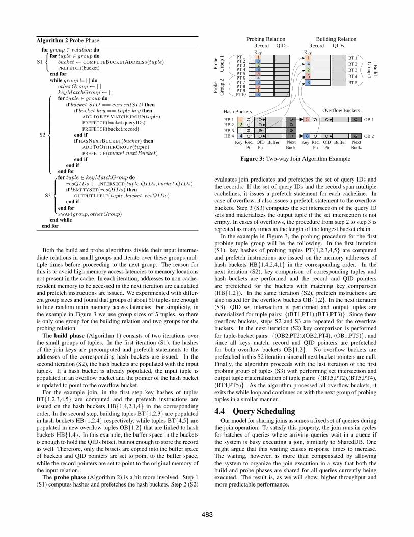
4.3 Join ProcedureNext we explain the build and probe phases of the hash join

algorithm in more detail. For clarification purposes we also providean example shown in Figure 3 and work through the example as weexplain the algorithms. The figure shows a simple setup with abuilding relation of 5 tuples, probing relation with 10 tuples andthe populated hash table.

482

Algorithm 2 Probe Phasefor group ∈ relation do

for tuple ∈ group dobucket← COMPUTEBUCKETADDRESS(tuple)S1

PREFETCH(bucket)end forwhile group != [ ] do

otherGroup← [ ]keyMatchGroup← [ ]for tuple ∈ group do

if bucket.SID == currentSID thenif bucket.key == tuple.key then

ADDTOKEYMATCHGROUP(tuple)PREFETCH(bucket.queryIDs)PREFETCH(bucket.record)

end ifS2

if HASNEXTBUCKET(bucket) thenADDTOOTHERGROUP(tuple)PREFETCH(bucket.nextBucket)

end ifend if

end forfor tuple ∈ keyMatchGroup do

resQIDs← INTERSECT(tuple.QIDs, bucket.QIDs)if !EMPTYSET(resQIDs) then

OUTPUTTUPLE(tuple, bucket, resQIDs)S3

end ifend forSWAP(group, otherGroup)

end whileend for

Both the build and probe algorithms divide their input interme-diate relations in small groups and iterate over these groups mul-tiple times before proceeding to the next group. The reason forthis is to avoid high memory access latencies to memory locationsnot present in the cache. In each iteration, addresses to non-cache-resident memory to be accessed in the next iteration are calculatedand prefetch instructions are issued. We experimented with differ-ent group sizes and found that groups of about 50 tuples are enoughto hide random main memory access latencies. For simplicity, inthe example in Figure 3 we use group sizes of 5 tuples, so thereis only one group for the building relation and two groups for theprobing relation.

The build phase (Algorithm 1) consists of two iterations overthe small groups of tuples. In the first iteration (S1), the hashesof the join keys are precomputed and prefetch statements to theaddresses of the corresponding hash buckets are issued. In thesecond iteration (S2), the hash buckets are populated with the inputtuples. If a hash bucket is already populated, the input tuple ispopulated in an overflow bucket and the pointer of the hash bucketis updated to point to the overflow bucket.

For the example join, in the first step key hashes of tuplesBT{1,2,3,4,5} are computed and the prefetch instructions areissued on the hash buckets HB{1,4,2,1,4} in the correspondingorder. In the second step, building tuples BT{1,2,3} are populatedin hash buckets HB{1,2,4} respectively, while tuples BT{4,5} arepopulated in new overflow tuples OB{1,2} that are linked to hashbuckets HB{1,4}. In this example, the buffer space in the bucketsis enough to hold the QIDs bitset, but not enough to store the recordas well. Therefore, only the bitsets are copied into the buffer spaceof buckets and QID pointers are set to point to the buffer space,while the record pointers are set to point to the original memory ofthe input relation.

The probe phase (Algorithm 2) is a bit more involved. Step 1(S1) computes hashes and prefetches the hash buckets. Step 2 (S2)

Pro

be

Gro

up 1

Probing RelationRecord QIDs

Build

Group 1

Building RelationRecord QIDs

8

12

4

14258

Hash Buckets Overflow Buckets

PT 1PT 2PT 3PT 4PT 5PT 6PT 7PT 8PT 9PT10

Key KeyBT 1BT 2BT 3BT 4BT 5

HB 1HB 2HB 3HB 4

OB 1

OB 2Key Rec.

PtrQIDPtr

NextBuck.

NextBuck.

5

8

1

5

1

8

8

8

5

4

2

Pro

be

Gro

up 2

Rec.Ptr

QIDPtr

KeyBuffer Buffer

Figure 3: Two-way Join Algorithm Example

evaluates join predicates and prefetches the set of query IDs andthe records. If the set of query IDs and the record span multiplecachelines, it issues a prefetch statement for each cacheline. Incase of overflow, it also issues a prefetch statement to the overflowbuckets. Step 3 (S3) computes the set intersection of the query IDsets and materializes the output tuple if the set intersection is notempty. In cases of overflows, the procedure from step 2 to step 3 isrepeated as many times as the length of the longest bucket chain.

In the example in Figure 3, the probing procedure for the firstprobing tuple group will be the following. In the first iteration(S1), key hashes of probing tuples PT{1,2,3,4,5} are computedand prefetch instructions are issued on the memory addresses ofhash buckets HB{1,4,2,4,1} in the corresponding order. In thenext iteration (S2), key comparison of corresponding tuples andhash buckets are performed and the record and QID pointersare prefetched for the buckets with matching key comparison(HB{1,2}). In the same iteration (S2), prefetch instructions arealso issued for the overflow buckets OB{1,2}. In the next iteration(S3), QID set intersection is performed and output tuples arematerialized for tuple pairs: {(BT1,PT1),(BT3,PT3)}. Since thereoverflow buckets, steps S2 and S3 are repeated for the overflowbuckets. In the next iteration (S2) key comparison is performedfor tuple-bucket pairs: {(OB2,PT2),(OB2,PT4), (OB1,PT5)}, andsince all keys match, record and QID pointers are prefetchedfor both overflow buckets OB{1,2}. No overflow buckets areprefetched in this S2 iteration since all next bucket pointers are null.Finally, the algorithm proceeds with the last iteration of the firstprobing group of tuples (S3) with performing set intersection andoutput tuple materialization of tuple pairs: {(BT5,PT2),(BT5,PT4),(BT4,PT5)}. As the algorithm processed all overflow buckets, itexits the while loop and continues on with the next group of probingtuples in a similar manner.

4.4 Query SchedulingOur model for sharing joins assumes a fixed set of queries during

the join operation. To satisfy this property, the join runs in cyclesfor batches of queries where arriving queries wait in a queue ifthe system is busy executing a join, similarly to SharedDB. Onemight argue that this waiting causes response times to increase.The waiting, however, is more than compensated by allowingthe system to organize the join execution in a way that both thebuild and probe phases are shared for all queries currently beingexecuted. The result is, as we will show, higher throughput andmore predictable performance.

483

The other alternative is to schedule queries immediately as theyarrive. This is common for systems that share scans such asIBM DB2 [18, 19], MonetDB [28], and is also used by CJoin [9]and Datapath [3]. The effect on join execution is that the buildand probe phases need to be executed concurrently in a pipelinefashion. The problem is in the redundant work to be done for aset of concurrently running queries, which is the first stage of thepipeline, i.e. the build phase. The effect on performance dependson the relative cost between the build and probe phases and theamount of sharing missed. The effect is further aggravated in casesof multi-way joins where there are multiple stages in the pipeline.

4.5 Query ID Set RepresentationAs mentioned previously, shared query execution introduces an

additional attribute for each intermediate tuple in the system. Thisattribute keeps information on which queries are interested in eachtuple. There are several ways to store and handle this attribute,each with advantages and disadvantages. One way to represent thisattribute is as an array of integers each of which represents the IDof the query that is interested in the tuple. The impact of this is thatthe size of the attribute is Ni · sint bytes where Ni is the numberof queries interested in the tuple and sint is the size of the integer.

Another way of representing the set of query IDs is to use a bitsetwhere each query in the system has a dedicated bit position in thebitset. For a certain tuple with a bitset B, and a query Q whose bitposition is i if the ith bit in B is 1 then the query is interested inthe tuple, and vice-versa if the bit is 0. The size of the attribute isthen the size of the bitset which is Ns

8bytes where Ns is the total

number of concurrently running queries.One factor affecting the performance trade-off between the two

methods is the ratio Avg(Ni)Ns

of average number of queries per tupleAvg(Ni) to the number of concurrent queries Ns. Bitsets workwell when this ratio is high or Ns is sufficiently low. Arrays workwell in cases where this ratio is low andNs is very high. In practice,we found that, for analytical workloads, bitsets perform better.

4.6 DiscussionMQJoin is similar to CJoin and Datapath in using bitsets to

handle the query ID set for each tuple, as well as the use of a hashbased algorithm.

An important difference to CJoin and Datapath is that in thosesystems the build and probe phases are executed concurrently. Asa result, the hash table is constantly updated for all incoming andoutgoing queries, which introduces extra work per query. In CJoin,for instance, the hash table is updated for each query individually,both when the query enters and exits the system. This works for starschemas and low concurrency cases where the effort required in thebuild phase is significantly lower than during the probe phase. InDatapath, colliding hash table entries from newly arrived querieswill be placed in the next available entry in the hash table. Thiscauses extra work to be done during probing and it is unclear howthe hash table is purged when queries finish. To minimize the workrequired for building, updating and clearing the hash table, our joinalgorithm runs in cycles, performing build and probe one after theother in each cycle. This allows us to share the build operationfor all queries that are being executed in the current cycle. At theend of each cycle we clear all data in the hash table by simplyincrementing the session ID number. This avoids replaying buildsubqueries to clear data from the hash table.

Another difference is in the micro-architectural properties of thealgorithm. SharedDB uses single-threaded join operators which isinefficient for analytical workloads on multi-core systems. Simi-larly, CJoin builds and updates the hash table in a single thread,

1. SELECT * FROM R, S WHERE R.A = S.A2. SELECT * FROM R LEFT OUTER JOIN S ON R.A = S.A3. SELECT * FROM R RIGHT OUTER JOIN S ON R.A = S.A4. SELECT * FROM R FULL OUTER JOIN S ON R.A = S.A5. SELECT * FROM R WHERE R.A IN (SELECT S.A FROM S)6. SELECT * FROM R WHERE R.A NOT IN (SELECT S.A FROM S)7. SELECT * FROM S WHERE S.A IN (SELECT R.A FROM R)8. SELECT * FROM S WHERE S.A NOT IN (SELECT R.A FROM R)

Figure 4: List of Queries Whose Join Can be Shared

which is inefficient if the build relations are not insignificantlysmall. This is another reason why CJoin is restricted to starschemas. Datapath uses a single hash table for all joins which isdivided in 64 regions with exclusive locks. To avoid contention onthese locks, it needs to update the hash table in two phases. Ouralgorithm parallelizes both build and probe phases and synchro-nizes build operations on a per bucket basis. We optimize for bothCPU and bandwidth efficiency by hiding random access latenciesthrough software prefetching and minimizing the number of ran-dom cachelines accessed per tuple. This makes the performanceof our algorithm comparable to that of the fastest published query-at-a-time join algorithms, something that none of the competingversions can do.

4.7 Sharing Execution for Other Join TypesThe algorithm we just described works for queries that require

inner joins. It can be extended to share execution for queriesthat also require (left, right, full) outer-joins and (anti) semi-joins,provided that they are all on the same equality predicate. Consider asimple schema of relations R(A int,B int) and S(A int, C int),and a shared join operator which builds the hash table with therelation S and probes with the relation R. Then consider the set ofqueries shown in Figure 4. To handle these queries, the algorithmis extended to perform additional operations on the bitsets duringprobing. These additional operations depend on the join type andcan be setting bits of individual queries to 1, conditional set to zero,or bitwise OR. This extension allows to answer queries 2, 4, 5, 6and 7. Another extension is to modify tuples’ bitsets in the hashtable during probing, and iterate over the build relation again afterprobing to output tuples which did not have a match in the probingrelation. This extension allows to answer queries 3, 4 and 8.

5. MULTI-WAY JOINSIn this section we describe how multiple join operations are

handled. As with the query-at-a-time approach, the shared joinapproach also requires an optimization decision on how to createquery plans involving multiple joins. The shared join optimizer notonly needs to decide the order of a multi-way join but also whichqueries’ execution should be shared. It can be undesirable to sharethe execution of some queries either for performance isolationreasons or if sharing would hurt overall performance.

Building such an optimizer is actually a non-trivial task and isout-of-scope of this paper. Recent work by Giannikis et al. [13] hasaddressed this problem and these techniques can also be applied toour approach. In this paper we focus on one end of the spectrum,that is to maximize sharing across all concurrent queries. While thismight not be always optimal or desirable, it provides a lower boundfor the performance of our approach. The ordering of the joins iscurrently done by hand. Next we explain how we maximize sharingfor queries with multi-way joins. The key challenge to address ishandling queries without common subplans. In this regard, we usetwo techniques: query plan equalization and global query batching.

484

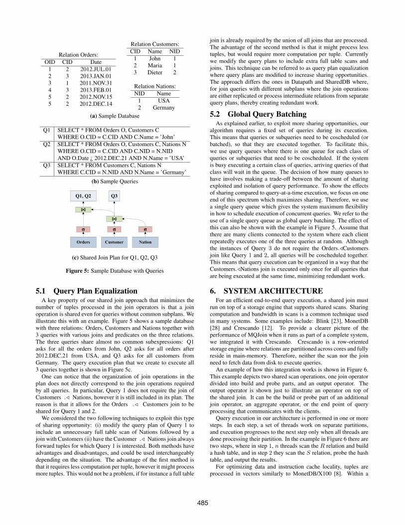
Relation Orders:OID CID Date

1 2 2012.JUL.012 3 2013.JAN.013 1 2011.NOV.314 3 2013.FEB.015 2 2012.NOV.155 2 2012.DEC.14

Relation Customers:CID Name NID

1 John 12 Maria 13 Dieter 2

Relation Nations:NID Name

1 USA2 Germany

(a) Sample Database

Q1 SELECT * FROM Orders O, Customers CWHERE O.CID = C.CID AND C.Name = ’John’

Q2 SELECT * FROM Orders O, Customers C, Nations NWHERE O.CID = C.CID AND C.NID = N.NIDAND O.Date ¿ 2012.DEC.21 AND N.Name = ’USA’

Q3 SELECT * FROM Customers C, Nations NWHERE C.CID = N.NID AND N.Name = ’Germany’

(b) Sample Queries

(c) Shared Join Plan for Q1, Q2, Q3

Figure 5: Sample Database with Queries

5.1 Query Plan EqualizationA key property of our shared join approach that minimizes the

number of tuples processed in the join operators is that a joinoperation is shared even for queries without common subplans. Weillustrate this with an example. Figure 5 shows a sample databasewith three relations: Orders, Customers and Nations together with3 queries with various joins and predicates on the three relations.The three queries share almost no common subexpressions: Q1asks for all the orders from John, Q2 asks for all orders after2012.DEC.21 from USA, and Q3 asks for all customers fromGermany. The query execution plan that we create to execute all3 queries together is shown in Figure 5c.

One can notice that the organization of join operations in theplan does not directly correspond to the join operations requiredby all queries. In particular, Query 1 does not require the join ofCustomers ./ Nations, however it is still included in its plan. Thereason is that it allows for the Orders ./ Customers join to beshared for Query 1 and 2.

We considered the two following techniques to exploit this typeof sharing opportunity: (i) modify the query plan of Query 1 toinclude an unnecessary full table scan of Nations followed by ajoin with Customers (ii) have the Customer ./ Nations join alwaysforward tuples for which Query 1 is interested. Both methods haveadvantages and disadvantages, and could be used interchangeablydepending on the situation. The advantage of the first method isthat it requires less computation per tuple, however it might processmore tuples. This would not be a problem, if for instance a full table

join is already required by the union of all joins that are processed.The advantage of the second method is that it might process lesstuples, but would require more computation per tuple. Currentlywe modify the query plans to include extra full table scans andjoins. This technique can be referred to as query plan equalizationwhere query plans are modified to increase sharing opportunities.The approach differs the ones in Datapath and SharedDB where,for join queries with different subplans where the join operationsare either replicated or process intermediate relations from separatequery plans, thereby creating redundant work.

5.2 Global Query BatchingAs explained earlier, to exploit more sharing opportunities, our

algorithm requires a fixed set of queries during its execution.This means that queries or subqueries need to be coscheduled (orbatched), so that they are executed together. To facilitate this,we use query queues where there is one queue for each class ofqueries or subqueries that need to be coscheduled. If the systemis busy executing a certain class of queries, arriving queries of thatclass will wait in the queue. The decision of how many queues tohave involves making a trade-off between the amount of sharingexploited and isolation of query performance. To show the effectsof sharing compared to query-at-a-time execution, we focus on oneend of this spectrum which maximizes sharing. Therefore, we usea single query queue which gives the system maximum flexibilityin how to schedule execution of concurrent queries. We refer to theuse of a single query queue as global query batching. The effect ofthis can also be shown with the example in Figure 5. Assume thatthere are many clients connected to the system where each clientrepeatedly executes one of the three queries at random. Althoughthe instances of Query 3 do not require the Orders./Customersjoin like Query 1 and 2, all queries will be coscheduled together.This means that query execution can be organized in a way that theCustomers./Nations join is executed only once for all queries thatare being executed at the same time, minimizing redundant work.

6. SYSTEM ARCHITECTUREFor an efficient end-to-end query execution, a shared join must

run on top of a storage engine that supports shared scans. Sharingcomputation and bandwidth in scans is a common technique usedin many systems. Some examples include: Blink [23], MonetDB[28] and Crescando [12]. To provide a clearer picture of theperformance of MQJoin when it runs as part of a complete system,we integrated it with Crescando. Crescando is a row-orientedstorage engine where relations are partitioned across cores and fullyreside in main-memory. Therefore, neither the scan nor the joinneed to fetch data from disk to execute queries.

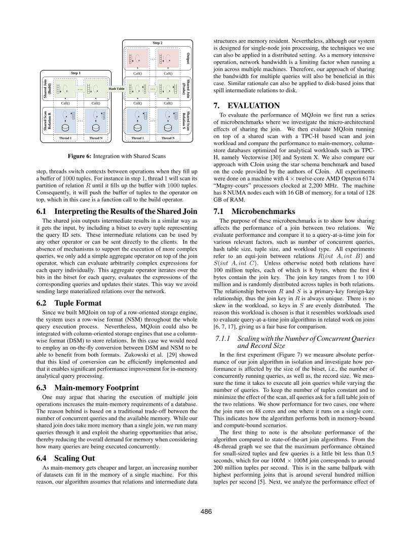
An example of how this integration works is shown in Figure 6.This example depicts two shared scan operations, one join operatordivided into build and probe parts, and an output operator. Theoutput operator is shown just to illustrate an operator on top ofthe shared join. It can be the build or probe part of an additionaljoin operator, an aggregate operator, or the end point of queryprocessing that communicates with the clients.

Query execution in our architecture is performed in one or moresteps. In each step, a set of threads work on separate partitions,and execution progresses to the next step only when all threads aredone processing their partition. In the example in Figure 6 there aretwo steps, where in step 1, n threads scan the R relation and builda hash table, and in step 2 they scan the S relation, probe the hashtable, and output the results.

For optimizing data and instruction cache locality, tuples areprocessed in vectors similarly to MonetDB/X100 [8]. Within a

485

Thread 1 Thread N Thread 1 Thread N

Step 2

Sh

ared

Jo

in

(Pro

be)

Sh

are

d J

oin

(Bu

ild

)

Step 1

Call()

Call()

Call()Call()

. . .

Call()

Call()

. . .

. . .

Ou

tpu

tS

ha

red S

can

Rela

tion

S

Sh

are

d S

can

Rel

ati

on

R

. . .. . . Hash Table

Figure 6: Integration with Shared Scans

step, threads switch contexts between operations when they fill upa buffer of 1000 tuples. For instance in step 1, thread 1 will scan itspartition of relation R until it fills up the buffer with 1000 tuples.Consequently, it will push the buffer of tuples to the operator ontop, which in this case is a function call to the build operator.

6.1 Interpreting the Results of the Shared JoinThe shared join outputs intermediate results in a similar way as

it gets the input, by including a bitset to every tuple representingthe query ID sets. These intermediate relations can be used byany other operator or can be sent directly to the clients. In theabsence of mechanisms to support the execution of more complexqueries, we only add a simple aggregate operator on top of the joinoperator, which can evaluate arbitrarily complex expressions foreach query individually. This aggregate operator iterates over thebits in the bitset for each query, evaluates the expressions of thecorresponding queries and updates their states. This way we avoidsending large materialized relations over the network.

6.2 Tuple FormatSince we built MQJoin on top of a row-oriented storage engine,

the system uses a row-wise format (NSM) throughout the wholequery execution process. Nevertheless, MQJoin could also beintegrated with column-oriented storage engines that use a column-wise format (DSM) to store relations. In this case we would needto employ an on-the-fly conversion between DSM and NSM to beable to benefit from both formats. Zukowski et al. [29] showedthat this kind of conversion can be efficiently implemented andthat it enables significant performance improvement for in-memoryanalytical query processing.

6.3 Main-memory FootprintOne may argue that sharing the execution of multiple join

operations increases the main-memory requirements of a database.The reason behind is based on a traditional trade-off between thenumber of concurrent queries and the available memory. While ourshared join does take more memory than a single join, we run manyqueries through it and exploit the sharing opportunities that arise,thereby reducing the overall demand for memory when consideringhow many queries are being executed concurrently.

6.4 Scaling OutAs main-memory gets cheaper and larger, an increasing number

of datasets can fit in the memory of a single machine. For thisreason, our algorithm assumes that relations and intermediate data

structures are memory resident. Nevertheless, although our systemis designed for single-node join processing, the techniques we usecan also be applied in a distributed setting. As a memory intensiveoperation, network bandwidth is a limiting factor when running ajoin across multiple machines. Therefore, our approach of sharingthe bandwidth for multiple queries will also be beneficial in thiscase. Similar rationale can also be applied to disk-based joins thatspill intermediate relations to disk.

7. EVALUATIONTo evaluate the performance of MQJoin we first run a series

of microbenchmarks where we investigate the micro-architecturaleffects of sharing the join. We then evaluate MQJoin runningon top of a shared scan with a TPC-H based scan and joinworkload and compare the performance to main-memory, column-store databases optimized for analytical workloads such as TPC-H, namely Vectorwise [30] and System X. We also compare ourapproach with CJoin using the star schema benchmark and basedon the code provided by the authors of CJoin. All experimentswere done on a machine with 4× twelve-core AMD Opteron 6174“Magny-cours” processors clocked at 2,200 MHz. The machinehas 8 NUMA nodes each with 16 GB of memory, for a total of 128GB of RAM.

7.1 MicrobenchmarksThe purpose of these microbenchmarks is to show how sharing

affects the performance of a join between two relations. Weevaluate performance and compare it to a query-at-a-time join forvarious relevant factors, such as number of concurrent queries,hash table size, tuple size, and workload type. All experimentsrefer to an equi-join between relations R(int A, int B) andS(int A, int C). Unless otherwise noted both relations have100 million tuples, each of which is 8 bytes, where the first 4bytes contain the join key. The join key ranges from 1 to 100million and is randomly distributed across tuples in both relations.The relationship between R and S is a primary-key foreign-keyrelationship, thus the join key in R is always unique. There is noskew in the workload, so keys in S are evenly distributed. Thereason this workload is chosen is that it resembles workloads usedto evaluate query-at-a-time join algorithms in related work on joins[6, 7, 17], giving us a fair base for comparison.

7.1.1 Scaling with the Number of Concurrent Queriesand Record Size

In the first experiment (Figure 7) we measure absolute perfor-mance of our join algorithm in isolation and investigate how per-formance is affected by the size of the bitset, i.e., the number ofconcurrently running queries, as well as, the record size. We mea-sure the time it takes to execute all join queries while varying thenumber of queries. To keep the number of tuples constant and tominimize the effect of the scan, all queries ask for a full table join ofthe two relations. We show performance for two cases, one wherethe join runs on 48 cores and one where it runs on a single core.This indicates how the algorithm performs both in memory-boundand compute-bound scenarios.

The first thing to note is the absolute performance of thealgorithm compared to state-of-the-art join algorithms. From the48-thread graph we see that the maximum performance obtainedfor small-sized tuples and few queries is a little bit less than 0.5seconds, which for our 100M × 100M join corresponds to around200 million tuples per second. This is in the same ballpark withhighest performing joins that is around several hundred milliontuples per second [5]. Next, we analyze the performance effect of

486

0

0.5

1

1.5

2

2.5

3

0 200 400 600 800 1000 0

10

20

30

40

50

60E

xec

uti

on

Tim

e (s

)

Cy

cles

per

Ou

tpu

t T

up

le

Query Scaling - 48 Threads

0

10

20

30

40

50

60

70

0 200 400 600 800 1000 0

200

400

600

800

1000

1200

1400

Ex

ecu

tio

n T

ime

(s)

Cy

cles

per

Ou

tpu

t T

up

leNumber of Queries

Query Scaling - Single Thread

8B Tup.64B Tup.

128B Tup.256B Tup.

Figure 7: Performance of a 100M×100M MQJoin for VariousNumber of Queries and Record Size

bitset and record size. Dealing with bitsets is an important source ofoverhead as it is not present in query-at-at-time join algorithms. Wenote that the difference in performance of sharing join execution foraround 500 concurrent queries instead of 1 is in general small andat most a factor of 2, the main reason being that 500 bits can stillbe accommodated in a single cacheline of 64 bytes.

The overhead of dealing with larger record sizes is also impor-tant, since queries might be interested in different attributes requir-ing for larger records to be projected and processed by the join op-erators. Similarly to the bitset size, the results show that increasingthe record sizes from 8 bytes to a cacheline size of 64 bytes has amarginal overhead. Enlargening the records to sizes bigger than acacheline of up to 256 bytes, however, adds a significant overheadand performance starts degrading linearly with the record size asmore non-cache resident memory has to be accessed per probe op-eration. To avoid this type of overhead several techniques can beused. One way is to employ standard techniques used in currentdatabases to avoid processing large records in the join such as datacompression and late materialization. Another way is to compressindividual records and have record-specific projection using onlythe attributes that are of interest to the queries the record belongs to.This technique prevents the increase in record size at the expense ofhaving more complex data dependent code. In our case, we foundthat such techniques are not necessary, since for the workloads weused the tuples did not exceed 64 bytes. And as mentioned before,the impact on performance in this case is negligibly small.

7.1.2 Effect of Hash Table SizeThe join is an operation which scales supralinear with relation

size. Typical breaking points are when the hash table no longer fitsin cache or no longer fits in main memory. When sharing a join theinput relations are a union of all relations required by the queries.Thus, knowing how exactly does a join scale with the size of a hashtable is important to understand the effect of sharing the join.

0

1

2

3

4

5

6

7

8

103

104

105

106

107

108C

ycl

es p

er P

robe

Oper

atio

n Relation Size Scaling - 48 Threads

L3 Cache

0

50

100

150

200

250

300

103

104

105

106

107

108C

ycl

es p

er P

robe

Oper

atio

n

Size of Build Relation (Tuples)

Relation Size Scaling - Single Thread

L3 Cache

Query-at-a-time JoinMQJoin - 1 Query

MQJoin - 512 Queries

Figure 8: Probe Performance versus Build Relation Size

In this paper we focus on main-memory databases. Thus, weconsider only the cases when a hash table fits in main-memory.We vary the size of relation R from 1,000 tuples to 100 milliontuples which covers the cases from when the hash table fits in L1

cache until it is much larger than L3 cache. As before, we measureperformance of full table joins for a join on 1 core and 48 cores.Since the size of the build relation is not constant, we only measurethe performance of the probe operation. We take measurements for3 different join cases. The first one is a query-at-a-time join forwhich we used our join algorithm without sharing support. Thesecond one is a shared join with only few queries (< 64). Finally,the third one is a shared join with 512 queries which is alreadyenough to feel the impact of the bitset size.

The most important thing to get from these graphs is the ratiobetween the lowest performance of the shared join and the highestperformance of a query-at-a-time join. The reason this is importantis that it depicts a worst-case scenario where the hash tables ofeach individual query fits in cache, but the union of all hash tablesdoes not fit in cache. The highest ratio in this case is around 6,which means in the worst case a probe operation will cost 6 timesmore for a shared join. However, it is important to note that sincethis corresponds to shared execution of 512 concurrent queries, theextra cost is compensated by the sharing.

Another observation to make is that the single-threaded caseis less sensitive to hash table size, and does not experience aperformance drop as the hash-table grows larger than the L3 cache.This means that the software prefetching technique we use is able tosuccessfully hide the large random main memory access latencieswhich occur when each hash table access is a cache miss.

7.1.3 Effects of Sharing the JoinIn the following experiment we illustrate the effect of sharing

the join for queries with predicates. We vary the selectivity aswell as the location of the predicates and we measure how muchtime it would take to execute a set of queries if they were to be

487

0.001

0.01

0.1

1

Ex

ecu

tio

n T

ime

(s)

Predicate on Build Relation

Predicate on Both Relations

Qu

ery

-at-

a-ti

me

Join

Predicate on Random Relation

0.001

0.01

0.1

1

1 10 100

Ex

ecu

tio

n T

ime

(s)

Number of Queries1 10 100

Number of Queries1 10 100

Sh

ared

Jo

in

Number of Queries

Predicate Selectivity:0.0001% 0.01% 1% 100%

Figure 9: Performance of MQJoin versus Query-at-a-time Join

executed with a shared join or one by one with a query-at-a-timejoin. We consider three types of queries with predicates: onewhere all queries have a predicate on one of the relations; onewhere all queries have predicates on both relations; and one wherehalf of the queries have a predicate on one relation and the otherhalf have a predicate on the other relation. We use the defaultrelations R and S both with 100 million tuples. A selectivity ofa predicate of, for instance 0.001% on relation R, means that thatquery selects randomly around 1,000 tuples from R. To avoidmeasuring the effects from scanning and evaluation of predicates,the input relations are precomputed both for the shared join and thequery-at-at-time join. Results are shown in Figure 9.

One important thing to emphasize from these results is that theexecution time of the shared join has a ceiling. This represents thepoint where the union of all tuples is the whole relation and thusshared join does a full table join. The performance then is constantuntil the size of the bitset gets high enough to make an impact.

For the first type of queries where all predicates are on onerelation a shared join almost always performs better than a query-at-a-time approach. This is true even in the cases when thepredicates are mutually exclusive for all queries, making the outputrelations mutually exclusive as well. The benefit in this case comesfrom sharing the probe relation, where every probing tuple is sharedfor all queries.

For the second type of queries where each query has a predicateon both relations we can see that a shared join is only beneficialif there are some common tuples between the queries. Due tothe randomness of the predicates in this setup, only the querieswith lower selectivity predicates share tuples as the number ofqueries increase. As the bitsets increase with more queries, theperformance of the shared join will suffer. However, if there are nocommon tuples between queries then the bitset will contain mostlyzeros so it will be easily compressible.

While the previous two cases were interesting to point out, weexpect that a realistic workload will consist of more diverse sets ofqueries. The worst case scenario for shared join is when there aretwo queries one with a predicate on one relation, while the other hasa predicate on the other relation. The shared join in this case will doa full table join, and the number of queries in this case required for

the shared join to do better than the query-at-at-time join dependsthe impact of the size of the hash table on the join, which is whatwe saw in Figure 8.

7.2 TPC-H BenchmarkThe TPC-H benchmark suite [1] consists of 22 analytical queries

most of which require heavy scans and joins on large portions ofdata. As we focus only on the scan and join operations of thequeries we took the TPC-H queries and extracted their scan and joinsubqueries. In order to avoid sending large materialized relationsover the network we included simple SUM aggregate on top of everyquery. To ensure that all attributes are projected during the joins asrequired in the original queries, we added all necessary attributes tothe SUM aggregate expression. For instance the transformed versionof Query 9 is shown in Listing 1

Listing 1: Transformed SQL version of Query 9SELECT SUM(

p s s u p p l y c o s t + l e x t e n d e d p r i c e + l d i s c o u n tl q u a n t i t y + s n a t i o n k e y + o t o t a l p r i c e )

FROM l i n e i t e m , p a r t , s u p p l i e r , p a r t s u p , o r d e r sWHERE l o r d e r k e y = o o r d e r k e yAND l p a r t k e y = p p a r t k e yAND l s u p p k e y = s s u p p k e yAND l p a r t k e y = p s p a r t k e yAND l s u p p k e y = p s s u p p k e yAND p name LIKE ’%[COLOR]% ’ ;

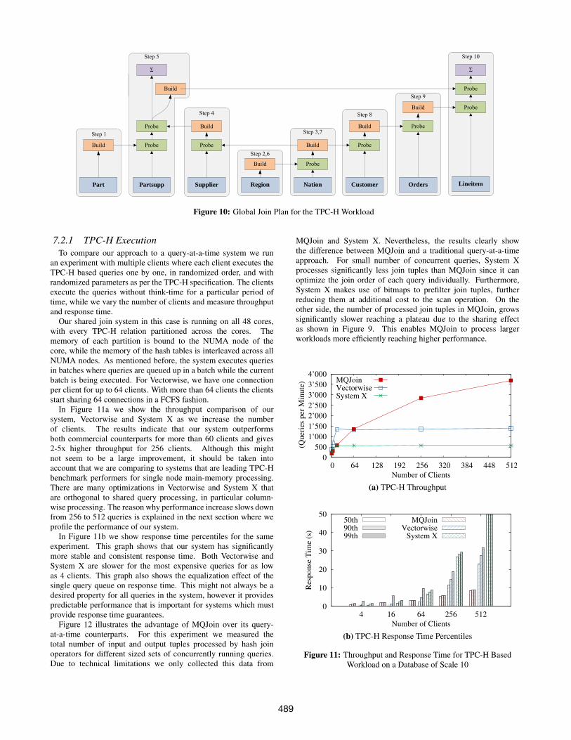
Furthermore, we removed any queries that required no joins,queries that contain more complex predicates which our sharedscan implementation does not yet support, and queries that requiredjoins other than equi-joins, which are not currently supported byour system. The final set of queries include 13 query templatesthat contained the scan and join subqueries of the following TPC-Hqueries: 2, 3, 5, 7, 8, 9, 10, 11, 14, 16, 17, 19, 20. For comparison,related work uses a smaller subset of TPC-H. Both QPipe andDatapath work with only 8 queries. The global operator plan that isused to process these queries is shown in Figure 10. This plan wascreated as described in Section 5 to maximize sharing for a batchof queries. The scale of the TPC-H data used was 10.

488

Lineitem

Probe

Probe

Σ

Step 10

Orders

Probe

Build

Step 9

Customer

Probe

Build

Step 8

Step 3,7

Nation

Probe

Build

Region

Build

Step 2,6

Partsupp

Probe

Probe

Build

Step 5

Σ

Part

Build

Step 1

Supplier

Probe

Build

Step 4

Figure 10: Global Join Plan for the TPC-H Workload

7.2.1 TPC-H ExecutionTo compare our approach to a query-at-a-time system we run

an experiment with multiple clients where each client executes theTPC-H based queries one by one, in randomized order, and withrandomized parameters as per the TPC-H specification. The clientsexecute the queries without think-time for a particular period oftime, while we vary the number of clients and measure throughputand response time.

Our shared join system in this case is running on all 48 cores,with every TPC-H relation partitioned across the cores. Thememory of each partition is bound to the NUMA node of thecore, while the memory of the hash tables is interleaved across allNUMA nodes. As mentioned before, the system executes queriesin batches where queries are queued up in a batch while the currentbatch is being executed. For Vectorwise, we have one connectionper client for up to 64 clients. With more than 64 clients the clientsstart sharing 64 connections in a FCFS fashion.

In Figure 11a we show the throughput comparison of oursystem, Vectorwise and System X as we increase the numberof clients. The results indicate that our system outperformsboth commercial counterparts for more than 60 clients and gives2-5x higher throughput for 256 clients. Although this mightnot seem to be a large improvement, it should be taken intoaccount that we are comparing to systems that are leading TPC-Hbenchmark performers for single node main-memory processing.There are many optimizations in Vectorwise and System X thatare orthogonal to shared query processing, in particular column-wise processing. The reason why performance increase slows downfrom 256 to 512 queries is explained in the next section where weprofile the performance of our system.

In Figure 11b we show response time percentiles for the sameexperiment. This graph shows that our system has significantlymore stable and consistent response time. Both Vectorwise andSystem X are slower for the most expensive queries for as lowas 4 clients. This graph also shows the equalization effect of thesingle query queue on response time. This might not always be adesired property for all queries in the system, however it providespredictable performance that is important for systems which mustprovide response time guarantees.

Figure 12 illustrates the advantage of MQJoin over its query-at-a-time counterparts. For this experiment we measured thetotal number of input and output tuples processed by hash joinoperators for different sized sets of concurrently running queries.Due to technical limitations we only collected this data from

MQJoin and System X. Nevertheless, the results clearly showthe difference between MQJoin and a traditional query-at-a-timeapproach. For small number of concurrent queries, System Xprocesses significantly less join tuples than MQJoin since it canoptimize the join order of each query individually. Furthermore,System X makes use of bitmaps to prefilter join tuples, furtherreducing them at additional cost to the scan operation. On theother side, the number of processed join tuples in MQJoin, growssignificantly slower reaching a plateau due to the sharing effectas shown in Figure 9. This enables MQJoin to process largerworkloads more efficiently reaching higher performance.

0

500

1’000

1’500

2’000

2’500

3’000

3’500

4’000

0 64 128 192 256 320 384 448 512

Thro

ughput

(Q

uer

ies

per

Min

ute

)

Number of Clients

MQJoinVectorwiseSystem X

(a) TPC-H Throughput

0

10

20

30

40

50

4 16 64 256 512

Res

ponse

Tim

e (s

)

Number of Clients

50th90th99th

MQJoinVectorwise

System X

(b) TPC-H Response Time Percentiles

Figure 11: Throughput and Response Time for TPC-H BasedWorkload on a Database of Scale 10

489

0

200

400

600

800

1000

1200

1400

64 128 192 256 320 384 448 512

Num

ber

of

Pro

cess

ed

Join

Tuple

s (M

illi

on)

Number of Queries

MQJoinSystem X

Figure 12: Number of Tuples Processed in Join Operations inMQJoin vs System X

7.2.2 Performance ProfilingIn the performance results in the previous experiment the through-

put no longer increased for MQJoin after a certain point. In thefollowing experiment we show the reason behind this. Figure 13shows the breakdown of CPU time spent in our system per opera-tor class while varying the number of concurrently running queries.The concurrent queries are a multiple of the set of 13 TPC-H basedqueries with randomized parameter values. The results shows that,as the number of queries in the batch increase, the scan operatorstake most of the CPU time. The reason for this is that, as shownpreviously, a shared join scales almost constantly with the numberof queries as soon as the point of doing full table joins is reached.On the other hand, scaling the evaluation of predicates is more dif-ficult and depends on workload parameters such as complexity andselectivity of the predicates.

7.2.3 Workload PropertiesSince we are running a workload with hundreds of concurrent

queries, it is important to understand the amount of overlap in thequeries and its effect on performance. For this reason we performedboth a static analysis of each of the 13 query templates and adynamic analysis on the workload as it is being executed in thesystem. The results show little overlap in the amount of data queriesare interested in and demonstrates the reason why MQJoin is ableto benefit from sharing opportunities in this case.

Table 1 shows the summary from the static workload analysiswith two key properties for each of the 13 query templates. Thenumber of possible predicate parameters indicate how many uniquequeries there are in a certain workload. For the largest workloadof 512 concurrent clients, this corresponds to around 40 queryinstantiations per template. As the table shows, only 3 of the 13templates have less than 40 possible parameter values, the smallest

0

1

2

3

4

5

6

64 128 192 256 320 384 448 512

CP

U T

ime

per

Core

(s)

Number of Queries

ScanJoin

Aggregate

Figure 13: CPU Time spent per Operator Class for TPC-HBased Workload

Table 1: Workload Properties: Selectivity and Number ofPossible Parameters per Query Template

Select. #Param. Select. #Param.

Q2 0.08% 1250 Q11 4% 25Q3 0.465% 155 Q14 0.277% 60Q5 4% 25 Q16 2% 3750Q7 0.064% 625 Q17 0.1% 1000Q8 0.0053% 18750 Q19 0.0028% 250Q9 5.26% 92 Q20 0.043% 2300Q10 4.16% 24

one having 24. The rest have many more possible parameter values,meaning that even in a set of 512 concurrent queries, the expectedamount of identical queries will be marginally small.

The selectivity values show the combined selectivity of thepredicates for each query template. The results show that themajority of the queries have a selectivity of less than 1 percent,which indicates possibly little overlap in the data of interest evenfor several hundred queries. This is confirmed by the results of ourdynamic workload analysis shown in Figure 14. In this experimentwe measured the average number of queries per tuple for differenttypes of intermediate results. The solid red line corresponds tothe intermediate results, which are the output of join operators andinput to aggregate operators. The very small amount of queries pertuple of around 1.4 for 100 queries and 2.6 for 400 queries confirmsthe small overlap in data mentioned before.

Unlike the output, the input to the join operators contains a largeroverlap in data with an average of 120 queries per tuple for 400concurrent queries. For this case we measured the average numberof queries per tuple in the intermediate results that are the outputof scan operators and input to join operators. As is also shown inFigure 14, the majority of this overlap comes from full table scans.This experiment demonstrates the benefits of sharing join executioneven for queries with a disjoint set of predicates, since there is stilla large overlap in the data that needs to be processed.

7.3 Comparison to CJoinAs the closest related work, we also compare our approach to

CJoin [9]. We use the same Star Schema Benchmark [21] workloadused to test CJoin. The data set has a scale of 100 and we use threeworkload types. The first two come from the same workload usedin the CJoin paper with the predicates on the dimension relationsset to 1% and 10% respectively. The third one uses the queries andselectivity as defined by the Star Schema Benchmark specification.We do not use queries 1.1, 1.2 and 1.3 as they contain predicateson the fact relation which is not supported by CJoin. Since wedo not support a group by operation, we used a corresponding

0

20

40

60

80

100

120

64 128 192 256 320 384 448 512

Num

ber

of

Quer

ies

per

Tuple

Number of Concurrent Queries

Join OutputScan Output

Scan Output (w/o Full Table Scans)

Figure 14: Amount of Data Overlap in Intermediate Results

490

1

10

100

1’000

10’000

1 10 100 1000

Med

ian

Res

po

nse

Tim

e (s

)

Number of Clients

1

10

100

1’000

10’000

100’000

1e+06

1 10 100 1000

Th

rou

gh

pu

t (Q

uer

ies

/ H

ou

r)

Number of Clients

MQJoin1% Selectivity

10% SelectivitySSB Predicates

CJoin

1% Selectivity10% SelectivitySSB Predicates

Figure 15: MQJoin and CJoin Performance for Star Schema Benchmark Dataset of Scale 100

sum operation for CJoin as well. To avoid any disk accesses forCJoin, we placed the underlying Postgres instance in a temporaryin-memory file system. For both systems, we varied the number ofclients and measured response time and throughput. Clients issuequeries one after another without think-time.

The results are shown in Figure 15. The first thing to noteis the large performance difference between the two systems.One reason is that CJoin was designed with a disk-resident factrelation in mind, and was run on a smaller machine with 8 cores.Although Postgres resides fully in main-memory, the streamingof the fact relation from Postgres to CJoin becomes a bottleneckand is not able to supply the CJoin operator running on 40+cores. Nevertheless, the main conclusion to draw from these resultscomes from the relative performance of the two systems as thenumber of clients increases. CJoin’s performance starts degradingsignificantly sooner as a result of missed sharing opportunities.Since CJoin updates the hash tables for each query as the queryarrives to the system, it misses out on sharing the build operation forconcurrent queries. As the number of clients increase, updating thehash tables becomes a bottleneck. The per query cost of buildingand updating the hash table is also a relevant factor. As shown in theresults, workloads with less selective or more complex predicateson the dimension relations aggravate the problem. It is also for thisreason why CJoin is suitable only in a star schema scenario.

8. CONCLUSIONSThis paper presented an algorithm that exploits the sharing

potential of join execution up to a very high level to meet thedemands of such workloads. The goal is achieved by usingtechniques that minimize redundant work across concurrent queriesand efficiently use the hardware resources such as CPU andmemory bandwidth. The resulting method handles significantlylarger workloads than the state-of-the-art and outperforms leadingmain-memory analytical databases by providing higher throughputand more stable and predictable response times.

9. REFERENCES[1] TPC-H Benchmark.

http://www.tpc.org/tpch/spec/tpch2.17.0.pdf.[2] M.-C. Albutiu, A. Kemper, and T. Neumann. Massively Parallel Sort-merge

Joins in Main Memory Multi-core Database Systems. PVLDB,5(10):1064–1075, June 2012.

[3] S. Arumugam, A. Dobra, C. M. Jermaine, N. Pansare, and L. Perez. TheDataPath System: a Data-centric Analytic Processing Engine for Large DataWarehouses. In Proc. SIGMOD 2010, pages 519–530, 2010.

[4] R. Avnur and J. M. Hellerstein. Eddies: Continuously Adaptive QueryProcessing. In Proc. SIGMOD 2000, pages 261–272, 2000.

[5] C. Balkesen, G. Alonso, J. Teubner, and M. T. Ozsu. Multi-core, main-memoryjoins: Sort vs. hash revisited. PVLDB, 7(1):85–96, 2013.

[6] C. Balkesen, J. Teubner, G. Alonso, and M. T. Ozsu. Main-memory hash joinson multi-core CPUs: Tuning to the underlying hardware. In Proc. ICDE 2013,pages 362–373, 2013.

[7] S. Blanas, Y. Li, and J. M. Patel. Design and Evaluation of Main Memory HashJoin Algorithms for Multi-core CPUs. In Proc. SIGMOD 2011, pages 37–48,2011.

[8] P. A. Boncz, M. Zukowski, and N. Nes. MonetDB/X100: Hyper-PipeliningQuery Execution. In Proc. CIDR 2005, pages 225–237, 2005.

[9] G. Candea, N. Polyzotis, and R. Vingralek. A scalable, predictable join operatorfor highly concurrent data warehouses. PVLDB, 2(1):277–288, Aug. 2009.

[10] S. Chen, A. Ailamaki, P. B. Gibbons, and T. C. Mowry. Improving Hash JoinPerformance Through Prefetching. In Proc. ICDE 2004, pages 116–, 2004.

[11] S. Chen, A. Ailamaki, P. B. Gibbons, and T. C. Mowry. Improving Hash JoinPerformance Through Prefetching. ACM Trans. Database Syst., 32(3), Aug.2007.

[12] G. Giannikis, G. Alonso, and D. Kossmann. SharedDB: Killing one ThousandQueries with One Stone. PVLDB, 5(6):526–537, Feb. 2012.

[13] G. Giannikis, D. Makreshanski, G. Alonso, and D. Kossmann. SharedWorkload Optimization. PVLDB, 7(6):429–440, Feb. 2014.

[14] S. Harizopoulos and A. Ailamaki. StagedDB: Designing Database Servers forModern Hardware. In In IEEE Data, pages 11–16, 2005.

[15] S. Harizopoulos, V. Shkapenyuk, and A. Ailamaki. QPipe: a SimultaneouslyPipelined Relational Query Engine. In Proc. SIGMOD 2005, pages 383–394,2005.

[16] R. Johnson, S. Harizopoulos, N. Hardavellas, K. Sabirli, I. Pandis, A. Ailamaki,N. G. Mancheril, and B. Falsafi. To Share or Not to Share? In Proc. VLDB2007, pages 351–362, 2007.

[17] C. Kim, T. Kaldewey, V. W. Lee, E. Sedlar, A. D. Nguyen, N. Satish,J. Chhugani, A. Di Blas, and P. Dubey. Sort vs. Hash Revisited: Fast JoinImplementation on Modern Multi-core CPUs. PVLDB, 2(2):1378–1389, Aug.2009.

[18] C. A. Lang, B. Bhattacharjee, T. Malkemus, S. Padmanabhan, and K. Wong.Increasing Buffer-Locality for Multiple Relational Table Scans throughGrouping and Throttling. In Proc. ICDE 2007, pages 1136–1145, 2007.

[19] C. A. Lang, B. Bhattacharjee, T. Malkemus, and K. Wong. IncreasingBuffer-locality for Multiple Index Based Scans through Intelligent Placementand Index Scan Speed Control. In Proc. VLDB 2007, pages 1298–1309.

[20] S. Manegold, P. Boncz, and M. Kersten. Optimizing Main-Memory Join onModern Hardware. IEEE Trans. on Knowl. and Data Eng., 14(4):709–730, July2002.

[21] P. O’Neil, B. O’Neal, and X. Chen. Star Schema Benchmark.http://www.cs.umb.edu/˜poneil/StarSchemaB.PDF.

[22] I. Psaroudakis, M. Athanassoulis, and A. Ailamaki. Sharing Data and Workacross Concurrent Analytical Queries. PVLDB, 6(9):637–648, July 2013.

[23] L. Qiao, V. Raman, F. Reiss, P. J. Haas, and G. M. Lohman. Main-memory ScanSharing for Multi-core CPUs. PVLDB, 1(1):610–621, Aug. 2008.

[24] V. Raman, G. Swart, L. Qiao, F. Reiss, V. Dialani, D. Kossmann, I. Narang, andR. Sidle. Constant-Time Query Processing. In Proc. ICDE 2008, pages 60–69,2008.

[25] T. K. Sellis. Multiple-query Optimization. ACM Trans. Database Syst.,13(1):23–52, Mar. 1988.

[26] A. Shatdal, C. Kant, and J. F. Naughton. Cache Conscious Algorithms forRelational Query Processing. In Proc. VLDB 1994, pages 510–521, 1994.

[27] P. Unterbrunner, G. Giannikis, G. Alonso, D. Fauser, and D. Kossmann.Predictable Performance for Unpredictable Workloads. PVLDB, 2(1):706–717,Aug. 2009.

[28] M. Zukowski, S. Heman, N. Nes, and P. Boncz. Cooperative Scans: DynamicBandwidth Sharing in a DBMS. In Proc. VLDB 2007, pages 723–734, 2007.

[29] M. Zukowski, N. Nes, and P. Boncz. DSM vs. NSM: CPU PerformanceTradeoffs in Block-oriented Query Processing. In Proc. DaMoN 2008, pages47–54, 2008.

[30] M. Zukowski, M. van de Wiel, and P. Boncz. Vectorwise: A VectorizedAnalytical DBMS. In Proc. ICDE 2012, pages 1349–1350, 2012.

491