mpls traffic engineering recovery mechanisms
TRANSCRIPT

CHAPTER 5
....,... '.......~~?0I\~.,,'~s~l~~i~iïÎ~.~...
MPLS Traffic EngineeringRecovery Mechanisms
Multi-Protocol Label Switching (MPLS) traffc engineering (TE) has encounteredan ineluctable success during the past years, which led to the development of a richset of MPLS TE recovery techniques.
This chapter starts with a refresher of the MPLS TE technology, followed bythe motivation for deploying such a technology in a data network. The recoverytechnques are then examined with the objective to provide a detailed description oftheir mode of operation and their respective pros and cons, the type of the networkdesign they preferably apply to, and aspects of design that operators fid importantfor deployment in their network.
Furthermore, various properties of each recovery technique are analyzed.
These properties are of the utmost importance when choosing a particular recoverytechnque in a network: the recovery time, the impact on scalabilty, the abilityto provide some quality-of-service (QoS) guarantees along the alternate path, andthe technique effciency with respect to the amount of bandwidth dedicated torecovery path. These are just a subset of the aspects covered for each recovery
technque.This chapter covers the default restoration mode of operation of MPLS TE, as
well as the global and local protection recovery schemes. A rich set of examples areprovided. throughout this chapter that ilustrate the mode of operation and howthose various recovery techniques can be deployed in a network. An entire section isdevoted to a complete set of case studies that show how an operator can use thoseMPLS recovery techniques to satisfy a set of recovery objectives while respectingnetwork constraints. It is worth highlighting that most of these case studies areinspired by existing or foreseen deployment scenarios. After a summary section, this
297
~ CHAPTER 5 MPLS Traffc Engineering Recovery Mechanisms
fist part of this chapter concludes with the standardization aspects of the MPLS TErecovery techniques. Then, the second part ofthis chapter is devoted to some advancedtopics of MPLS recovery. The aim of those two sections is to cover in detail thesignaling aspects of MPLS local protection (Section 5.14) and the interesting topicof the backup path computation (Section 5.15) and may be skipped by the readerwithout alterig the good understanding of the MPLS recovery techniques. Finallythis chapter concludes with a section that describes various related topics of research.
5.1 MPLS Traffic Engineering Refresher
In this section, we first provide a brief refresher on the notion of traffc engineering.Then the terminology specific to MPLS TE is shown through an example, and afterhaving reviewed the main components of MPLS TE, we detail the motivation fordeploying MPLS TE in a network.
5.1.1 Traffic Engineering in Data Networks
One of the major challenges of network design has always been traffc engineering;that is, how to route the traffc so network resources are effciently used. The term"efficiently" requires some explanations though. An obvious objective of networkdesign is to avoid congestion. If the network is fully congested, traffc engineeringcannot really help and the network has to be upgraded (i.e., bandwidth and/orswitchig/routing capacities must be added). On the other hand, if some regions ofthe network are congested while others have spare capacity, then trying to alleviatethe congestion spots by rerouting some flows along an alternate path (where
capacity is available) certainly helps.In other words, TE defies how flows should be routed to effciently use
network resources. Even in the absence of congestion, a more optimal traffc loadbalance may help increase the QoS. For instance, suppose that some links are usedat 60% capacity (on the average), which strictly speaking cannot be considered acongested link whereas other links are loaded at 10%. It is worth noting that delay-sensitive traffc traversing a link loaded at 60% may experience some undesirabledelay and jitter, especially without queuing mechanisms. Thus, achieving a bettertraffc load balance with the objective of minimizing the average link utilizationmight be another motivation for TE.
Traffc engineering is not per se specific to MPLS. Various network types havebeen using TE methods like public voice networks, A TM, Frame Relay, and InternetProtocol (IP).
The Classic Fish Problem
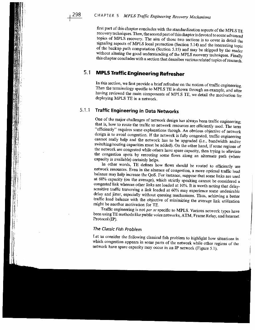
Let us consider the following classical fish problem to highlight how situations inwhich congestion appears in some parts of the network while other regions of thenetwork have spare capacity may occur in an IP network (Figure 5.1).

5.1 MPLS Traffc Engineering Refresher ~.""" ~ .~. - '". ~ A. _..._-_.~. ,,- ~-- - .
, - Path North: R3-R4-RS-R8
- Path South: R3-R4-RS-R8
Routing Decision
Based on the IPDestination Address All Links Have a Metric = 1
Figure 5.1 The classic "fish problem."
Figure S.L depicts two IP routers Rl and R2 sending traffc to the routerR8 (and beyond). Both Rl and R2 wil compute the shortest path to reach R8using a routing protocol like Open Shortest Path First (OSPF) or IntermediateSystem to Intermediate System (IS-IS). Because all the links have an equal metric ofi, the flows from Rl and R2 to R8 wil both follow the same path ("north"). If
thesum of their traffc exceeds the bandwidth capacity of the path "north" (R3-R4-RS), this will result in some congestion, although some capacity is stil availablealong the path "south." Changing the link metric in this case wil not help becauseIP routing protocols base their routing decision on the IP destination address. Sowhether a packet whose destination is R8 is received from Rl or R2, it wil be
routed by R3 along the same path. Another option in this very simple case is to setup the link metric so the north and south paths have an equal cost to use loadbalancing, but real networks are more complicated, and if other nodes areconnected to routers R4, RS, R6, and R7, load balancing becomes much morechallenging to achieve.
That said, TE with IP routing is of course possible and has already been
discussed in Chapter 4.One solution to obtain better resource utilization is to use tunneling techniques
between source(s) and destination(s) so intermediate nodes do not participate in therouting decision. ATM was extensively used to reach that goal; ATM permanentvirtual circuits (PVCs)/switched virtual circuits (SVCs) are established betweenswitches with characteristics based on the traffic requirements of each circuit(e.g., bandwidth and QoS). ATM PVCs/SVCs are routed based on the networkresources and link costing using off-line or on-line path computation methods (e.g.,Private Network-Network Interface (PNNIJ). Then, once a packet (encapsulated inATM cells) is routed onto an ATM PVC, it strictly follows the ATM PVC path.
~ CHAPTER 5 MPLS Traffc Engineering Recovery Mechanisms
!,f¡",,
:1
~ r i
i~
i~
Although relatively efficient to improve network bandwidth usage, there are severalsignificant drawbacks with this approach:
. An additional layer (A TM) has to be managed and maintained in the
network (A TM), which implies additional cost in terms of equipment andnetwork operation.
. The number of routing adjacencies maintained by each router is potentiallyvery high because every router has a number of routing neighbors equal tothe number of routers in the mesh, which introduces some routing protocolscalability limitations. Indeed, a mesh ofn routers requires for each of themto maintain n adjacencies and the route computation (shortest path first(SPFJ) is also increased signifcantly.
This is where MPLS TE comes into play. MPLS TE is also a "tunneling"mechanism using TE Label Switch Paths (TE LSPs; the termnology TE LSP isdetailed hereafter), which are established between pair of routers.
Each TE LSP has its own set of constraints-like bandwidth, affiities, andrerouting constraints, to mention a few-and the network topology and resourcesare taken into account along with the set of constraints to compute the TE LSPpath that satisfies the set of requirements. Different path computation methods canbe used to achieve that objective: distributed (each router is responsible for thecomputation of its TE LSP path) or centralized (an off-lie tool performs the pathcomputation of all the TE LSPs in the network). Then once a TE LSP is established,IP packets are routed onto the TE LSP and strictly follow the computed path;intermediate routers do not make any routing decision.
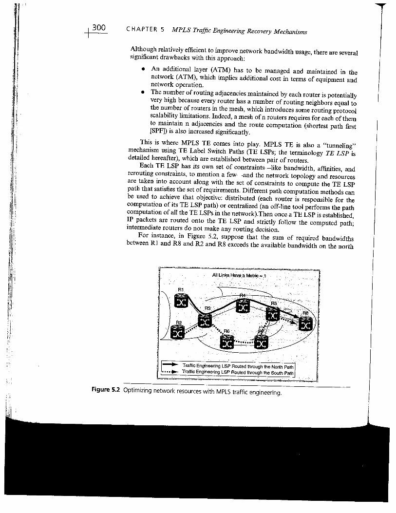
For instance, in Figure 5.2, suppose that the sum of required bandwidthsbetween Rl and R8 and R2 and R8 exceeds the available bandwidth on the north
. ",... ".""~ _. '..a
~ Traffic Engineering LSP Routed through the North Path
, . . .. ~ Traffic Engineering LSP Routed through the South Path
~. n ~_._'. _. '-'---"~,",' '~'-~"--"." -,,_.. .-, ~._.
Figure 5.2 Optimizing network resources with MPLS traffic engineering.
5.1 MPLS Traffc Engineering Refresher ~path (R3-R4-R5). By using MPLS TE, once the TE LSP between Rl and R8 isestablished, R2 figures out that the bandwidth available on the north path isnot sufficient to accommodate its traffc demand and selects the south path(R2-R3-R6-R 7-R5-R8) to establish its TE LSP. This allows better network resourceutilization and avoids traffc congestion.
Note that compared to the previous case with an A TM overlay network, justone layer is required (IP/MPLS). Moreover, routers are not required to maintainrouting adjacencies over TE LSP. It is important to note that MPLS TE is a controlplane reservation protocol, so this is fundamentally a Call Admission Control(CAC) mechanism. In other words, when a TE LSP is set up, no particularresources in the data plane are reserved. The purpose of MPLS TE is to ensurethat a TE LSP is not routed along a path where other TE LSPs have already
reserved the bandwidth. For instance, on an OC3 link, if three TE LSPs havealready been reserved a total bandwidth of 120 Mbps, the remaining available
bandwidth (not already reserved in the control plane) is 35 Mbps and a TE LSPrequiring more than 35 Mbps will have to be routed along another path. This is incontrast to IP in which IP packets are routed along the shortest path without
considering the traffc flow and available resources along this path.
.
5.1.2 Terminology
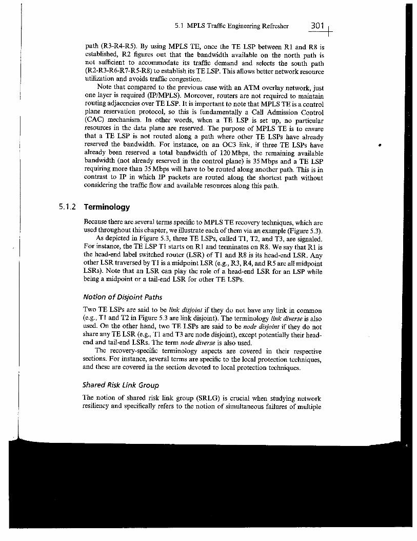
Because there are several terms specifc to MPLS TE recovery techniques, which areused throughout this chapter, we ilustrate each of them via an example (Figure 5.3).
As depicted in Figure 5.3, three TE LSPs, called Tl, T2, and T3, are signaled.For instance, the TE LSP Tl starts on Rl and termnates on R8. We say that Rl isthe head-end label switched router (LSR) of Tl and R8 is its head-end LSR. Anyother LSR traversed by Tl is a midpoint LSR (e.g., R3, R4, and R5 are all midpointLSRs). Note that an LSR can play the role of a head-end LSR for an LSP whilebeing a midpoint or a tail-end LSR for other TE LSPs.
Notion of Disjoint Paths
Two TE LSPs are said to be link disjoint if they do not have any link in common(e.g., Tl and T2 in Figure 5.3 are link disjoint). The terminology link diverse is alsoused. On the other hand, two TE LSPs are said to be node disjoint if they do notshare any TE LSR (e.g., Tl and T3 are node disjoint), except potentially their head-end and tail-end LSRs. The term node diverse is also used.
The recovery-specifc terminology aspects are covered in their respectivesections. For instance, several terms are specifc to the local protection techniques,and these are covered in the section devoted to local protection techniques.
Shared Risk Link Group
The notion of shared risk link group (SRLG) is crucial when studying networkresiliency and specifically refers to the notion of simultaneous failures of multiple
~ CHAPTER 5 MPLS Traffc Engineering Recovery Mechanisms
. .."' -J- .~--~ - ~ ,,' - '.-n -.-.. ~ ..
TE LSP(Taffc ËngineeringLabel Swiched Path)
Head'End LSR
Mid-Point LSÀ
Figure 5.3 Illustration of MPLS traffic engineering recovery.
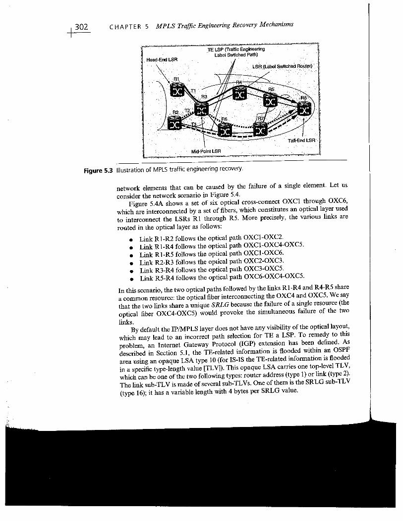
network elements that can be caused by the failure of a single element. Let usconsider the network scenario in Figure 5.4.
Figure 5.4A shows a set of six optical cross-connect OXCi through OXC6,which are interconnected by a set of fibers, which constitutes an optical
layer used
to interconnect the LSRs R1 through R5. More precisely, the various links arerouted in the optical layer as follows:
. Link RI-R2 follows the optical path OXC1-0XC2.
. Link RI-R4 follows the optical path OXC1-0XC4-0XC5.
. Link RI-R5 follows the optical path OXCI-OXC6.
. Link R2-R3 follows the optical path OXC2-0XC3.
. Link R3-R4 follows the optical path OXC3-0XC5.
. Link R5-R4 follows the optical path OXC6-0XC4-0XC5.
In this scenario, the two optical paths followed by the links RI-R4 and R4-R5 sharea common resource: the optical fiber interconnecting the OXC4 and OXC5. We saythat the two links share a unique SRLG because the failure of a single resource (theoptical fiber OXC4-0XC5) would provoke the simultaneous failure of the twolinks.
By default the IP/MPLS layer does not have any visibility of the optical layout,
which may lead to an incorrect path selection for TE a LSP. To remedy to thisproblem, an Internet Gateway protocol (IGP) extension has been defied. Asdescribed in Section 5.1, the TE-related information is flooded within an OSPFarea using an opaque LSA type 10 (for IS-IS the TE-related information is floodedin a specific type-length value (TL V)). This opaque LSA carries one top-level TL V,which can be one of the two following types: router address (type 1) or link (type 2).The link sub-TLV is made of several sub-TLVs. One of them is the SRLG sub-TLV
(type 16); it has a variable length with 4 bytes per SRLG value.

5.1 MPLS Traffc Engineering Refresher l2~ . w. - - .. .... .. .."- . .~.~.~ -. -,',~'-'-..,..
Shared Risk Link Group
. Optical Layer
OXC2 OXC3
OXC6
- ..-.---_..., -.- ,-, -_.~
Figure 5.4 Shared risk link group.
~ Important notes:
. A link may belong to multiple SRLGs.
. The IGP extensions allow carrying the SRLG values. On the other hand,having the knowledge of the underlying opticallSONET-SDH topology isnot always possible. Indeed, an operator may rely on another carrier toprovide optical lambda, and in that case, the SP does not always have theknowledge of the actual physical path and the potential SRLG. Moreover,an optical path may be dynamic and so its path may change over the time.This requires updating the SRLG value each time a change occurs if theSRLG changes also.
Notion of SRLG disjoint: A TE LSP is said to be SRLG disjoint from a link L or anode R if and only if its path does not include any link or node that is part of theSRLG of that L or R. For instance, back Figure 5.4, a TE LSP T1 following thepath RI-R2-R3-R4 is SRLG disjoint from the link RI-R4. Two TE LSPs are saidto be SRLG disjoint if the respective set of links they traverse do not have anySRLG in common.
5.1.3 MPLS Traffic Engineering Components
The aim of this section is to review the main components of MPLS TE:
1. Configuration of TE LSP on head-end LSR: The first step consists of config-uring the TE LSPs' attributes on the head-end LSR. Various attributes can beconfigured like the destination (address of the tail-end LSR), the requiredbandwidth, the required protection/restoration, the affnities, and others.
'i IIIi i¡¡
i f
!
!¡:
I:, ,¡ :
~ CHAPTER 5 MPLS Traffc Engineering Recovery Mechanisms
2. Topology and resource information distribution: To compute a path obeyingthe set of specified constraint(s), the head-end LSR needs to gather top-ology and resource information. Note that this applies only to situations inwhich the TE LSPs path is dynamically computed by each LSR (alsoreferred to as distributed or on-line path computation) by contrast withcentralized or offline path computation in which the LSPs' path is computedby an off-line tool. In such a case, the topology and resource information isdistributed by a lin state routing protocol (OSPF or IS-IS) with
TE extensions that reflect links characteristics and reservation states. TETLVs have been defied and are carred within an LSP for IS-IS and TEopaque LSA type 10 for OSPF to flood the reservation states and otherparameters.
3. TE LSP computation: As already stated, the computation of aTE LSP pathcan either be performed by an off-line tool or on-line. In the former case, anexternal tool simultaneously computes all the TE LSPs paths according tothe network resources. In the latter case, every router (LSR) uses its resourceand topology database (IS-IS or OSPF), takes into account the set ofrequirements of the TE LSP, and computes the shortest path satisfying theset of constraints usually using a constraint shortest path first (CSPF)algorithm. Various types of CSPFs can be used.
4. TE LSP setup: Once the path of aTE LSP has been computed, the head-endLSR signals the TE LSP by means of the Resource Reservation Protocol(RSVP) signaling protocol with the corresponding set of extensions defiedin (RSVP-TEl For instance, in Figure 5.3, Rl computes a path for the LSPT1: Rl-R3-R4-R5-R8 based on Tl's attributes and the network andresources topology information disseminated by the routing protocol.Once Tl's path is computed, Tl is signaled by RSVP-TE. TE LSPs arethen signaled, maintained (refreshed) and potentially torn down using vari-ous RSVP messages: Path, Resv, Path Error, Path Tear, Reservation Error,Resv Confation, and Resv Tear. Also, various new objects have beendefied in (RSVP-TE) for the purpose of MPLS TE, for example, to allocatelabels to TE LSPs that will then be used in the MPLS data plane. Note thatlabels are assigned in the upstream direction using RSVP messages (Resvmessage) and intermediate LSRs are programmed accordingly. Forinstance, when the TE LSP Tl is signaled, labels are assigned by LSRs inthe upstream direction: R8 provides a label to R5, R5 provides a label to R4,and so on.
Note: It is worth mentioning that RSVP has often been criticized for its scalabilty,in particular the number of states required in the network. As a matter of fact,currently deployed networks can handle thousands of RSVP TE reservations (TELSPs) on a single router without any problem. Moreover, various protocolenhancements have been defied (see (REFRESH-REDUCTION)) to furtherincrease the scalability, if needed. Finally, MPLS TE can be deployed with multiplelevels of hierarchies, if required, in very large networks.

5.1 MPLS Traffc Engineerig Refresher ~5. Packet forwarding: Once a TE LSP is set up, the head-end LSR can
update its routing table and start using TE LSP to forward IP packets.A label of 32 bits is pushed onto the IP packet, which is then label switchedacross the network (intermediate routers do not make any routing decision).
5.1.4 Notion of Preemption in MPLS Traffic Engineering
There is one interesting property called "preemption" defined in MPLS TE, whichdeserves to be slightly elaborated in the chapter because upon network elementfailure, preemption mechanisms may be triggered. (RSVP- TE) defines the notionof preemption or priority for a TE LSP. This parameter is signaled in theSESSION-ATTRIBUTE object of the RSVP TE Path message (more precisely,the RFC defies two priorities known as the "setup" and "holding" priorities,which define the priority of a TE LSP with respect to taking and holding resources,respectively).
When a new TE LSP is signaled, an LSR considers the admission of thisnewly signaled TE LSP by comparing the requested bandwidth with the bandwidthavailable at the priority specified in the setup priority. If the requested bandwidthis available but this requires preempting other TE LSPs having a lowerpriority, then the newly signaled TE LSP is admitted and one or more TE LSPswith a lower priority are preempted. Note that the selection of the set oflower priority TE LSPs to be preempted is a local decision and is generallyimplementation specifc. More details of preemption policies can be found in(pREEMPTION-POL).
The preemption process implies the set of followig actions for each preemptedTE LSP:
. The corresponding local RSVP states are cleared and the traffc is no longerforwarded.
. Messages are sent both upstream (RSVP Path Error message) and
downstream (RSVP Resv Error) so all the states corresponding to thepreempted TE LSP are cleared along its path. Then the head-LSR LSR ofa preempted TE LSP intiates a TE reroute procedure as detailed earlier toreroute the TE LSP along another path.
This means that hard preemption is by nature a disruptive mode. So the concept ofsoft preemption has been introduced in (SOFT-PREEMPTION) and proposes adifferent mode of preemption. If a TE LSP must be preempted to accommodate ahigher priority TE LSP requests, the preempting LSR performs the followingactions:
. The preempting LSP signals to the respective head-end LSR the need toreroute the TE LSP in a nondisruptive fashion (so-called "make beforebreak" procedure).
. The local states of the soft preempted TE LSP are not cleared and no RSVPPath Error/RSVP Error messages are sent.

~ CHAPTER 5 MPLS Traffc Engineering Recovery Mechanisms
Hence, the preempting node keeps forwarding the traffc of a soft preempted TELSP for a certain period. This gives a chance for the soft preempted TE LSPs head-end LSR to reroute their TE LSPs along an alternate path without disrupting traffcflow.
It is worth pointing out that this implies to temporary provoke reservationoverbooking on some links because until the soft preempted TE LSPs are reroutedby their respective head-end LSR, the sum of admitted bandwidth is higher than themaxium allowed. Note that some algorithms can be carefully designed to preempthard preemptabié2 TE LSPs first. Moreover, appropriate MPLS Diffserv mecha-nisms can be used to make sure that high-priority traffc is served adequately.
5.1.5 Motivations for Deploying MPLS Traffic Engineering
Once the concept of TE and the main components of MPLS TE have beenreviewed, it is time to highlight the various motivations for deploying MPLS TEin a network.
1. Bandwidth optimization: As pointed out in Section 5.1, MPLS TE can bedeployed to achieve better network resource utiliation, usually referred toas bandwidth optimization.
2. Strict QoS guarantees: Another motivation for deploying MPLS TE in anetwork is to enforce strict QoS guarantees for various service types includ-ing sensitive traffic flows like voice, video, and circuit emulation. As alreadymentioned, MPLS TE acts on the control plane and as such takes care of therouting decision. For instance, consider a network with a single class ofservice (CoS), MPLS TE allows an operator to reduce the average andmaximum link utilization. Hence, a direct implication is that the probabilityof traffc queuing delay is decreased, which correlates with a better QoS.
Another example is the case of a network with multiple classes of service.Making sure that appropriate treatment of sensitive flows is performed inthe data plane requires various mechanisms like marking, queuing, andcongestion avoidance in the data plane. In such networks, MPLS TE willallow control over the proportion of high-priority traffc versus medium-and low-priority traffc on a per-link basis, which wil increase the QoS.
Although this has already been highlighted, to provide QoS guaranteesbetween two nodes, specific actions must be taken in the IP/MPLS dataplane, implementing the Differentiated Services (Diffserv) modeL. Indeed,MPLS TE is responsible for finding a path obeying a set of constraints, butonce the packets are sent onto that TE LSP, each node along the path has toserve the packet appropriately according to the required CoSo
3. Fast recovery: Several mechanisms for MPLS TE are described throughoutthis chapter, allowing for fast recovery along with other requirements likeQoS protection during failure. Those mechanisms have been generating a
62The hard/soft preemptable property of a TE LSP is explicitly signaled in RSVP Path message.
5.2 Analysis of the Recovery Cycle l2growing interest for MPLS TE, and the sole interest for fast convergence,even if bandwidth optimization or strict QoS guarantees are not required,may justify the deployment of MPLS TE. Several large networks havedeployed MPLS TE to benefit from the set of fast recovery mechanisms.
The aim of the previous short paragraph was to introduce the motivation ofdeploying MPLS TE in a network: bandwidth optimization, strict QoS guarantees,and fast recovery. They are of course nonexclusive. For example, consider an IP/MPLS network where the resource utilization is not optimal and fast recovery isdesired. Then MPLS TE with, for instance, any fast recovery technique described inthis chapter can be deployed. Another example is an IP/MPLS network where strictQoS guarantees are required for the voice traffc, for instance, as well as fastrecovery for the virtual private networking (VPN) traffc and the voice traffc.Finally, as already pointed out, MPLS TE can be deployed for the sole motivationof benefiting from fast recovery. Consider an overprovisioned network in whichneither bandwidth optimization nor strict QoS guarantees are necessary (QoSguarantee is achieved by overprovisioning), but fast recovery is a must. ThenMPLS TE is a good candidate for its fast recovery property.
5.2 Analysis of the Recovery Cycle
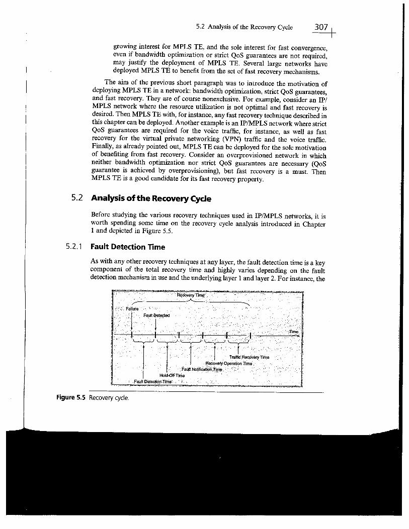
Before studying the various recovery techniques used in IP/MPLS networks, it isworth spending some time on the recovery cycle analysis introduced in Chapter1 and depicted in Figure 5.5.
5.2.1 Fault Detection Time
As with any other recovery techniques at any layer, the fault detection time is a keycomponent of the total recovery time and higWy varies depending on the faultdetection mechanism in use and the underlying layer i and layer 2. For instance, the
Figure 5.5 Recovery cycle.
~ CHAPTER 5 MPLS Traffc Engineering Recovery Mechanisms
fault detection time can vary from a few tens of milliseconds when two LSRs areinterconnected via a SONET/SDH VC or an opticallightpath to a few hundreds ofmillseconds or seconds when hello mechanisms are required. (Section 4.3 in Chap-ter 4 has been entirely devoted to the important aspects of failure profie and faultdetections aspects.)
5.2.2 Hold-Off Timer
A hold-off timer can be very useful if the underlying layer has a recovery scheme.Those aspects of multilayer protection/restoration strategies are covered in detail inChapter 6. In a nutshell, consider, for instance, a multilayer network where fastrecovery mechanisms are implemented both at the optical layer and at the MPLSlayer. Then, when the failure occurs, one should generally avoid any racing condi-tions where both recovery mechanisms simultaneously try to perform a reroutealong an alternate path. In that case, a bottom-up timer-based approach can beadopted, in which the MPLS layer wil wait for a hold-off timer to expire beforetrying to perform a reroute, to give the optical layer a chance to restore the failedresources. If the optical layer does not succeed in restoring the failed resource beforethe hold-off timer expires, the MPLS recovery mechanism wil be triggered torestore the failed resource at the MPLS layer (the interlayer recovery mechanismsare more extensively discussed in Chapter 6).
5.2.3 Fault Notification Time
To perform traffc recovery, an LSR must first be informed of the failure. As we wilsee in this chapter, depending on the MPLS TE recovery mechanism used, thetraffc recovery may be performed on the node imediately upstream to the failureor on the head-end LSR (the LSR originating the TE LSP); we call the faultindication signal (FIS) the signal of the failure to the node in charge of performngthe traffc recovery. Hence, once the fault has been detected by an LSR R, the PIS ispropagated until reaching an LSR that has the ability to reroute the TE LSPaffected by the failure. The fault notifcation time (time for the PIS to be receivedby the node in charge of the traffic recovery) wil vary depending on whether therecovery technque is local or global, as shown in Chapter i, Section 1.54.
It is usually desirable to guarantee through appropriate scheduling on thevarious LSRs that the PIS receives the proper QoS, to mimie and guaranteethe fault notifcation time. For instance, as mentioned in Chapter 4, the IGPflooding should be prioritized. In addition, IGP and RSVP messages should bequeued appropriately and of course should never be dropped in the case of conges-tion. Refer to Chapter 4, Section 4.5, for further details on QoS mechanisms.
RSVP Reliable Messaging
As we saw in the Chapter 4, IGP updates are always sent in reliable mode; this isinherent to link state routing protocols. By contrast, RSVP messages are sent bydefault in nonreliable mode. So a loss of a Path Error message (which is used to
5.2 Analysis of the Recovery Cycle ~report an LSP failure to upstream nodes) may significantly increase the faultnotification time, especially if the IGP has not been tuned to provide fast notifica-tion (see Chapter 4 for details). (REFRESH-REDUCTION) proposes a mechanismto send RSVP messages in reliable mode.
Two additional RSVP objects are defined: the MESSAGE-ID and the MES-SAGE-ID-ACK objects. Each RSVP message sent in reliable mode contains aunique MESSAGE-ID object and is acknowledged by a MESSAGE-ID-ACKobject (note that it may be piggybacked to any other RSVP messages or toan RSVP acknowledgment message). The retransmission of a nonacknowledgedmessage for which an explicit acknowledgment had been requested is based onan exponential back-off procedure; when an LSR has to send a message inreliable mode, it inserts a MESSAGE-ID object in the RSVP message and sets aparticular flag in the MESSAGE-ID header called the ACK-Desired flag.Upon receiving the RSVP message, a neighboring LSR will send back anRSVP message containing a MESSAGE-ID-ACK object. When the message isacknowledged, the transmission procedure is termnated. If the sending LSR doesnot receive any acknowledgment before a dynamic timer has elapsed, the messageis retransmitted. The dynamic timer Tk is exponentially increased until a maxiumvalue is reached. Tk is fist set to an initial retransmission value (generally a
short value).
For example, let us suppose that a message is sent for the first time, and Tk = Tlis set to initial timer (the recommended value is 500ms).
. If the message is not acknowledged after Tl, then it is retransmitted.Otherwise the procedure is stopped.
. Then Tk is set to Tk-¡* (1+delta) (the recommended value for delta is 1).
. The maximum value for k is set to a fied value (k = 3 is recommended).
In sumary, the sending LSR waits 500ms and then retransmits the message,then waits for the 500ms*2, then 500ms*4 with exponential increased waitingtimes. If the maxium retransmission value is set to 3, the message is no longerretransmitted after three trials.
5.2.4 Recovery Operation Time
Any recovery technique involves a set of actions to be completed. This includespotential synchronization between network elements to coordinate.
5.2.5 Traffic Recovery Time
The traffc recovery time represents the time between the last recovery action and
the time the traffc is completely recovered. Each component described earlier isanalyzed for the various recovery techniques described in this chapter. We just sawa brief description of each phase of the recovery cycle.
There are multiple types of MPLS TE recovery techniques (Table 5.1):
~ CHAPTER 5 MPLS Traffc Engineering Recovery Mechanisms
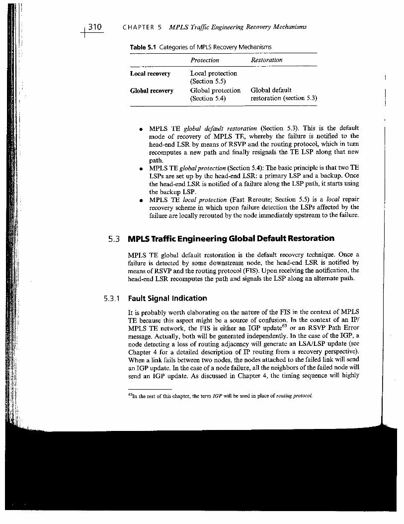
Table 5.1 Categories of MPLS Recovery Mechanisms
Protection Restoration
Local recovery Local protection(Section 5.5)Global protection(Section 5.4)
Global defaultrestoration (section 5.3)
Global recovery
. MPLS TE global default restoration (Section 5.3). This is the defaultmode of recovery of MPLS TE, whereby the failure is notified to thehead-end LSR by means of RSVP and the routing protocol, which in turnrecomputes a new path and fially resignals the TE LSP along that newpath.
. MPLS TE global protection (Section 5.4): The basic principle is that two TELSPs are set up by the head-end LSR: a priary LSP and a backup. Oncethe head-end LSR is notified of a failure along the LSP path, it starts usingthe backup LSP.
. MPLS TE local protection (Fast Reroute; Section 5.5) is a local repairrecovery scheme in which upon failure detection the LSPs affected by thefailure are locally rerouted by the node imediately upstream to the failure.
5.3 MPLS Traffic Engineering Global Default Restoration
MPLS TE global default restoration is the default recovery technique. Once afailure is detected by some downstream node, the head-end LSR is notifed bymeans of RSVP and the routing protocol (FIS). Upon receiving the notifcation, thehead-end LSR recomputes the path and signals the LSP along an alternate path.
5.3.1 Fault Signal Indication
It is probably worth elaborating on the nature of the PIS in the context of MPLSTE because this aspect might be a source of confusion. In the context of an IP/MPLS TE network, the PIS is either an IGP update63 or an RSVP Path Errormessage. Actually, both wil be generated independently. In the case of the IGP, anode detecting a loss of routing adjacency will generate an LSA/LSP update (seeChapter 4 for a detailed description of IP routing from a recovery perspective).
When a link fails between two nodes, the nodes attached to the failed link will sendan IGP update. In the case of a node failure, all the neighbors of the failed node willsend an IGP update. As discussed in Chapter 4, the timing sequence wil highly
63In the rest of this chapter, the term IGP wil be used in place of routing protocol.
5.3 MPLS Traffc Engineering Global Default Restoration ~depend on the failure detection time and IGP parameter tuning. Moreover, everynode detecting a failure wil also generate an RSVP Path Error message sent to eachhead-end LSR having a TE LSP traversing the failed resource. For instance, inFigure 5.3, if the link R3-R4 fails, as soon as the node R3 detects the link failure, itsends a notification (RSVP Path Error message) to Rl, the head-end LSR of T1because T1 traverses the failed link. In addition, an IGP update wil be sent by boththe nodes R3 and R4 to reflect the new topology. Again, the timing sequencedepends on the IGP tuning (see Chapter 4). Usually, the RSVP Path Error messageis received by the head-end LSRs within a few tens of milliseconds so generallybefore the IGP update, but regardless of which FIS is fist received, the head-endLSR wil get notified. As pointed out in Section 5.2, the FIS delivery is of the utmostimportance with MPLS global default restoration, because it triggers the reroutingof the affected LSPs by the head-end LSR.
5.3.2 Mode of Operation
When a TE LSP is configured on a head-end LSR, its set of attributes is specifed:destination (IP address of the tail-end LSR), bandwidth, priority, protection!restoration requirements, and other MPLS TE parameters. As far as the recoveryis concerned, an important parameter is the TE LSP path. As mentioned in Section5.1, the path of aTE LSP can be computed in either a distributed or a centralizedfashion. In the former case, the configuration does not specify any particular pathand the head-end LSR dynamically computes the LSP path, taking into account theconstraints and available resources in the network. In the latter case, the path forthe TE LSP is statically configured on the head-end LSR. Some MPLS TE imple-mentations allow the configuration of both options with an order of preference.
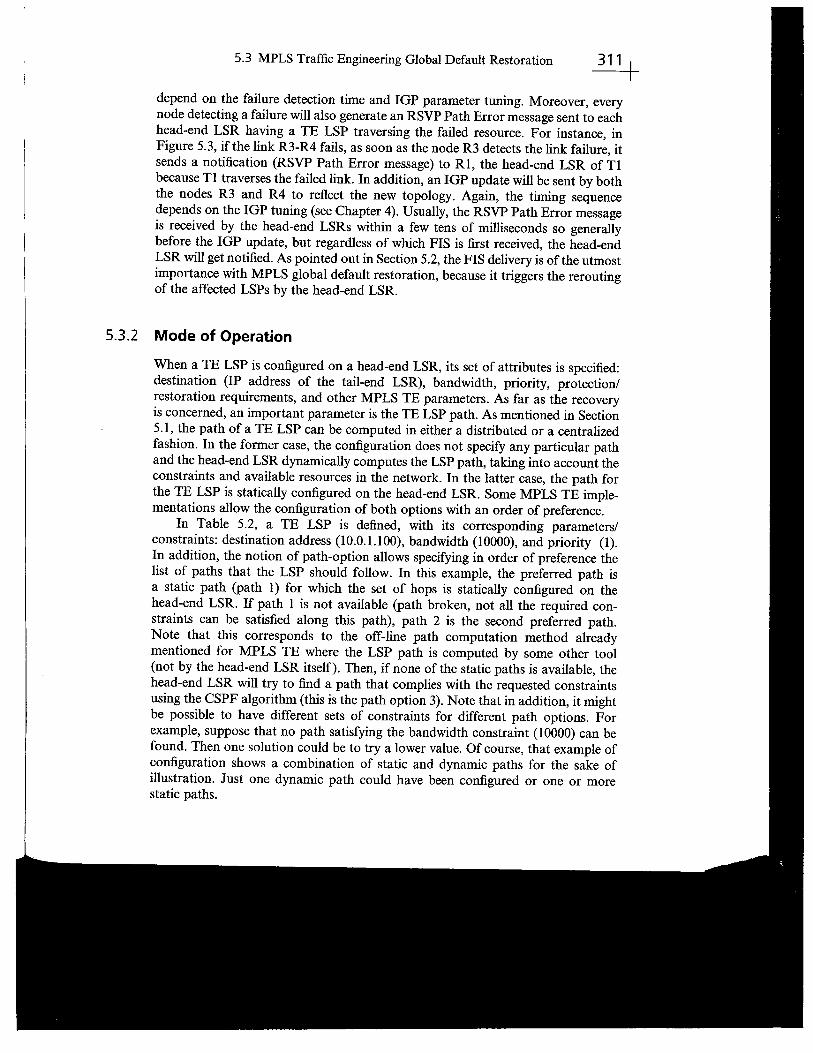
In Table 5.2, a TE LSP is defined, with its corresponding parameters/constraints: destination address (10.0. I. 00), bandwidth (10000), and priority (1).In addition, the notion of path-option allows specifying in order of preference the
list of paths that the LSP should follow. In this example, the preferred path isa static path (path I) for which the set of hops is statically configured on the
head-end LSR. If path 1 is not available (path broken, not all the required con-straints can be satisfied along this path), path 2 is the second preferred path.
Note that this corresponds to the ofT-line path computation method alreadymentioned for MPLS TE where the LSP path is computed by some other tool(not by the head-end LSR itself). Then, if none of the static paths is available, thehead-end LSR will try to fid a path that complies with the requested constraintsusing the CSPF algorithm (this is the path option 3). Note that in addition, it mightbe possible to have different sets of constraints for different path options. Forexample, suppose that no path satisfying the bandwidth constraint (10000) can befound. Then one solution could be to try a lower value. Of course, that example ofconfiguration shows a combination of static and dynamic paths for the sake ofilustration. Just one dynamic path could have been confgured or one or morestatic paths.
F CHAPTER 5 MPLS Traffc Engineering Recovery Mechanisms
Table 5.2 An example of MPLS Traffic Engineering TE LSP Configuration
interface Tunnellip unnumbered LoopbackO
no ip directed-broadcasttunnel destination 10.0.1.00tunnel mode mpls traffc-engtunnel mpls traffc-eng priority 1 itunel mpls traffc-eng bandwidth 10000
tunnel mpls traffc-eng record-routetunel mpls traffic-eng path-option i explicit name pathltunnel mpls traffic-eng path-option 2 explicit name path2tunel mpls traffic-eng path-option 3 dynamic
Path 1 = p92.170.14.2, 192.170.10.1, 192.170.4.5)
Path2 = p92.170.13.2, 192.170.17.1, 192.170.20.5)
Recovery Cycle with Global Default Restoration
The mode of operation of global default restoration is relatively simple: When thehead-end LSR is informed of the link/node failure, if an alternate path is specifed,the head-end LSR wil check to see whether the configured path satisfies theconstraints for the TE LSP. If so, the TE LSP is reestablished along that path. Ifno preconfgured path is specifed on the head-end router and if configued as such,then it triggers a new path computation for the set of affected TE LSPs, callng theCSPF process (this exactly corresponds to the example in Table 5.2: If a notifcationis received reporting that path 1 is unavailable, the head-end LSR tries to determinewhether it can use path 2, and if path 2 is not valid for some reason, it tries tocompute a path itself).
Note 1: Various existing MPLS TE implementations allow relaxing con-straint(s) upon failure, which might sometimes be necessary. A slightly morecomplicated example could be given in which for each path option, a set ofdifferent constraints is specifed. For instance, consider a network with rela-tively high link utilization in terms of bandwidth reservation; a major nodefailure may cause the inability for several TE LSPs to find an alternative path.In this case, one of the options is to relax some constraints, like the bandwidthconstraint so the TE LSP can be routed. There is one undesirable side effectthough: Allowing a TE LSP to be rerouted as a 0 bandwidth TE LSP impliesthat traffc will flow over this tunnel without any CAC. Thus, no bandwidth canbe guaranteed in this case. There are also various constraints aTE LSP can beconfigured to support. Bandwidth is just one of them. Another example isaffiities. This allows, for instance, to ensure some TE LSPs will avoid particu-lar network resources, using some bit masks. This can be seen as color. As an
"ii~
,.11"!i~
';Iir!
i';,i
il.i
:~ j
Iii'1\ii
¡riIi
'ii!i ~
":;
~i
~!:;:
I''."I;
~ .
,',Ii'
CI:
'.,
f"ii,

5.3 MPLS Traffic Engineering Global Default Restoration --example, some network links might be colored in red (with red meaning "highpropagation delay" or "poor quality"). This affiity link property is propa-gated through IGP TE extensions (see (OSPF-TE) and (IS-IS-TED. This way, aTE LSP carrying very sensitive traffc like voice-over-IP (VoIP) wil be config-ured so red links are excluded from the path selection. In such a case, a majornetwork failure may imply for the affected TE LSP to be non-reroutablewithout crossing one or several red links. In this case, it might be desirable torelax the affnity constraint.
Note 2: A large proportion of deployed MPLS TE networks rely on distributedcomputation in which no static path is confgured; in this case, just a dynamicpath is configured and the head-end just recomputes a new path based on theLSP constraints and its knowledge of the network and resource topology
information provided by the IGP.
A usual question is: What is the CSPF duration time? And the systematic
answer is: That depends. Indeed, the CSPF duration time is a function of thenetwork size and the CSPF algorithm in use. Finding the shortest constraint pathin a very large network obviously requires more time than in a small network.Furthermore, the CSPF complexity may be variable depending on the algorithm inuse. Finally, the router CPU should also be taken into account. That said, in anorder of magnitude, an average CSPF computation time using a classic CSPFalgorithm on a network with hundreds of nodes rarely exceeds a few milliseconds.It is worth noting that one CSPF must be triggered per affected TE LSP. Indeed, ifN LSPs starting on a head-end LSR Rl traverse a failed link, Rl wil have tocompute a new path for each of them.
Once a new path has been found and computed, the TE LSP is signaled alongthe new path. The fial operation before any traffc can be routed over the newly
signaled TE LSP consists of updating the routing table for the destinations that canbe reached via the TE LSP.
5.3.3 Recovery Time
Providing hard numbers is not a realistic exercise because a signifcant number offactors influence the rerouting time, but we describe the different components of therecovery cycle with global default restoration through an example. Figure 5.6 showsthe different steps of the recovery cycle with MPLS TE global default restoration.
Step 1: The link R3-R4 fails, and an FIS (RSVP and IGP update) is sent to thehead-end LSR. As already pointed out, the sequence timing of IGP update andthe RSVP Path Error depends of many factors. The receipt of one of them issuffcient for the head-end LSR to be notified of the failure.Step 2: The FIS is sent to the head-end LSR. Note that the propagation delaymight be nonnegligible and is made up of two components: the propagationdelay (on wide area networks; this can be on the order of tens of millisecondsand can become as large as 100 ms between two continents where the opticalpath can be very long) and the queuing and processing delays for the PIS to

~ CHAPTER 5 MPLS Traffic Engineering Recovery Mechanisms
New Path Comp~tation '
(I For the Set qf AffeGied. TE LSPs . T1:(D,
Figure 5.6 Event scheduling in the case of link/node failure with MPLS TE reroute.
reach the head-end router. As mentioned in Section 5.2, an appropriatemarking and scheduling in the forwarding path is highly recommended toensure that the queuing and processing delays are both minimized.Step 3: Upon receiving the failure notification, the head-end LSR (Rl in thisexample) tries to fid an alternate path satisfying the set of constraints for eachTE LSP affected by the failure.Step 4: The TE LSP is signaled along the new path. The RSVP signaling set uptime is also made of several components: the propagation delay along the path(round trip) and the queuing and processing delays at each hop in both direc-tions (upstream and downstream).Step 5: The routing table of Rl is updated to use the newly signaled LSP.
In conclusion, because the different components of the recovery time are highlydependent of the network characteristics, the resulting recovery time may vary froma few milliseconds to hundreds of miliseconds, sometimes a few seconds. TestingMPLS traffic reroute in a lab made of a few routers will probably result in a veryshort convergence time (a few milliseconds); indeed, the propagation delays arenegligible, as is the FIS processing delay. The CSPF computation is also very shortbecause the network size is limited, and finally the set up time will also be negligible.In contrast, a network with 1000 nodes, links with high propagation delays, andhundreds of TE LSPs to reroute wil require a much more significant amount oftime to converge.
5.4 MPLS Traffic Engineering Global Path Protection
MPLS TE global path protection (also usually referred to as path protection) is aglobal 1:1 protection recovery mechanism. As defied in Chapter i, Section 1.5.4,this implies that the head-end LSR performs the rerouting (global recovery) and apresignaled backup LSP is used (protection) if the protected LSP fails.
5.4 MPLS Traffc Engineering Global Path Protection ~5.4.1 Mode of Operation
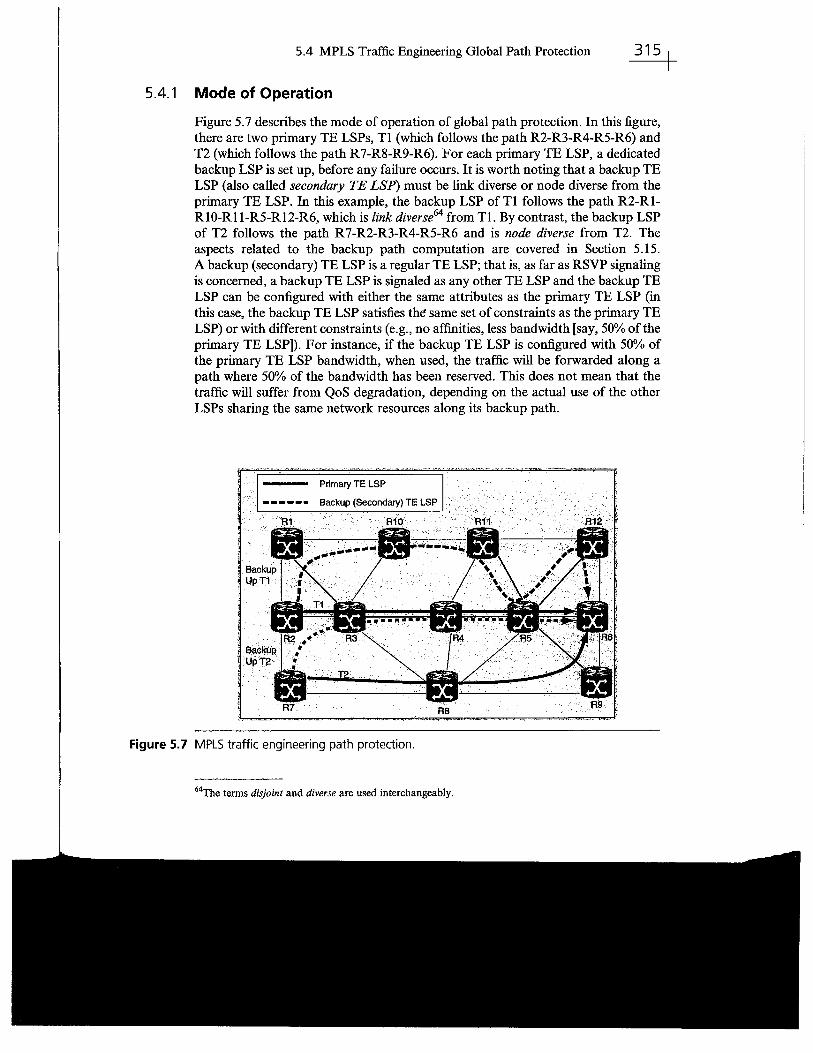
Figure 5.7 describes the mode of operation of global path protection. In this figure,there are two primary TE LSPs, T1 (which follows the path R2-R3-R4-R5-R6) andT2 (which follows the path R7-R8-R9-R6). For each primary TE LSP, a dedicatedbackup LSP is set up, before any failure occurs. It is worth noting that a backup TELSP (also called secondary TE LSP) must be link diverse or node diverse from thepriary TE LSP. In this example, the backup LSP of T1 follows the path R2-Rl-R10-Rll-R5-R12-R6, which is link diverse64 from Tl. By contrast, the backup LSPof T2 follows the path R7-R2-R3-R4-R5-R6 and is node diverse from T2. Theaspects related to the backup path computation are covered in Section 5.15.A backup (secondary) TE LSP is a regular TE LSP; that is, as far as RSVP signalingis concerned, a backup TE LSP is signaled as any other TE LSP and the backup TELSP can be configured with either the same attributes as the primary TE LSP (inthis case, the backup TE LSP satisfies the' same set of constraints as the priary TELSP) or with different constraints (e.g., no affinities, less bandwidth (say, 50% ofthepriary TE LSPD. For instance, if the backup TE LSP is confgued with 50% ofthe priary TE LSP bandwidth, when used, the traffic will be forwarded along apath where 50% of the bandwidth has been reserved. This does not mean that thetraffc wil suffer from QoS degradation, depending on the actual use of the otherLSPs sharing the same network resources along its backup path.
.'.'.''',-- -.,.. -"- ._,.--_. . '" ~ -'-'''_.
-, .~-.~. --" r- -,
Figure 5.7 MPLS traffic engineering path protection.
~e terms disjoint and diverse are used interchangeably.
!
~"": i~ ~ CHAPTER 5 MPLS Traffc Engineering Recovery Mechanisms
The mode of operation is quite straightforward: Once the failure is detected bysome downstream node, an FIS is sent to the head-end LSR of each affected LSP
(by affected LSP, we mean each LSP traversing the failed resource).Note that all the aspects related to the FIS delivery described in Section 5.3
identically apply here because both the global default restoration and the globalpath protection rely on the FIS delivery to trigger an LSP recovery.
Then upon receiving the FIS, the head-end LSR imediately switches thetraffc onto the backup TE LSP and updates its routing table accordingly.
5.4.2 Recovery Time
Compared to global default restoration, no routing computation has to bedone "on the fly" to find an alternate route for the failed TE LSP. Moreover,with global path protection, the backup tunnel is already signaled, so no signalinground is required to set up the backup TE LSP. It is important to note that thesavig in convergence time is predominately provided by the pre signaling of theTE LSP.
5.5 MPLS Traffic Engineering Local Protection
,I
.I!
.'1,\
iil
i II"II!'!
,:1
Mter a brief section introduction to the specifc terminology used for MPLS TElocal protection, we describe the principle and mode of operation of two localprotection techniques called MPLS TE Fast Reroute. The last section describestwo deployment strategies of local protection recovery techniques. Note that theterms MPLS TE local protection and Fast Reroute are used interchangeablythroughout this chapter.
5.51 Terminology
,i j
" I
. i
We begin this section by defiing the termnology specifc to MPLS TE FastReroute through an example (Figure 5.8).
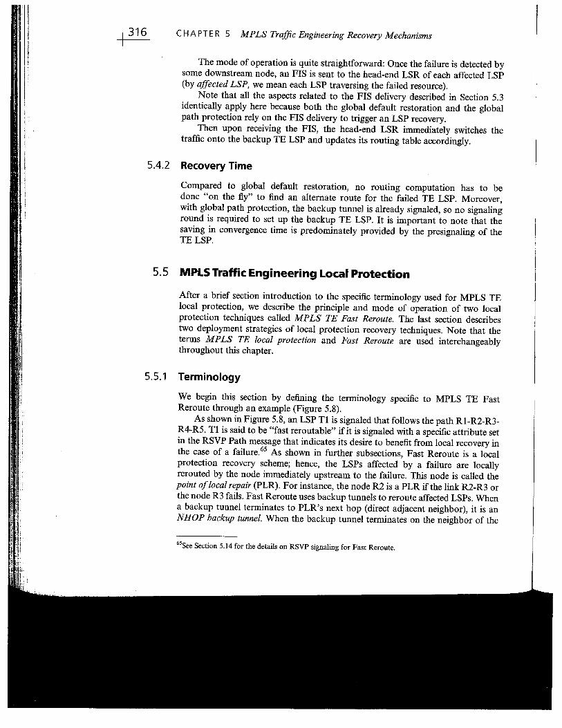
As shown in Figure 5.8, an LSP T1 is signaled that follows the path RI-R2-R3-R4-R5. T1 is said to be "fast reroutable" if it is signaled with a specifc attribute setin the RSVP Path message that indicates its desire to benefit from local recovery inthe case of a failure.65 As shown in further subsections, Fast Reroute is a localprotection recovery scheme; hence, the LSPs affected by a failure are locallyrerouted by the node imediately upstream to the failure. This node is called thepoint of local repair (PLR). For instance, the node R2 is a PLR if the link R2-R3 orthe node R3 fails. Fast Reroute uses backup tunnels to reroute affected LSPs. Whena backup tunnel terminates to PLR's next hop (direct adjacent neighbor), it is anNHOP backup tunnel. When the backup tunnel termnates on the neighbor of the
'i Hj ';
i
H
¡¡
65See Section 5.14 for the detais on RSVP signaling for Fast Reroute.
5.5 MPLS Traffc Engineering Local Protection ~If:)
3
J
e
e
ge
e
Figure 5.8 Terminology (MPLS local protection).
~
.1
se
y 5.5.2
PLR's neighbor, the backup tunnel is an NNHOP backup tunnel. Back to ourexample, Bl is an NHOP backup tunnel of the PLR R2 and B2 is an NNHOPbackup tunnel of R2. The node where the backup tunnel termnates is called themerge point (MP); hence, R4 is the MP of B2. Finally, a fast-reroutable LSP is saidto be protected at a node R if there exists a backup tunnel that can be used in thecase of a failure. T1 is protected at R2 by Bland B2.
The termnology of detour merge point uséd in one Fast Reroute technique(one-to-one protection) is discussed in Section 5.14.
Principles of Local Protection Recovery Techniques
t
We use the generic term MPLS TE Fast Reroute or Fast Reroute to describe localprotection techniques. There are two techniques of Fast Reroute (both are localprotection techniques) that are described in this chapter:
. Facility backup (also referred to as bypass)
. One-to-one backup (also referred to as detour)
t1
.1
Y
e
r
Although the terminology might appear diffcult to understand, the termnologyused in this section is in line with the corresponding standardized documents.
Both methods described are local repair techniques using local protection:
. Local: In the case of a link or node failure, a TE LSP is rerouted by the node
that is immediately upstream to the failed link or node. Compared to theglobal default restoration and global path protection where the TE LSP isrerouted by the head-end LSR, in the case of local protection, the protectedLSP is rerouted at the closest location upstream to the failure. This presentsthe very significant advantage of eliminating the need for the FIS to bereceived by the head-end LSR to reroute the affected TE LSP along analternate path.
1
1
e

~ CHAPTER 5 MPLS Traffc Engineering Recovery Mechanisms
. Protection: As seen in the Chapter 1, with protection recovery mechanisms,
a backup resource is preallocated and signaled before the failure. With bothlocal protection recovery methods (facilty backup and one-to-one backup),the backup LSPs are established before the failure occurs. When a failureoccurs and is detected, every protected TE LSP traversing the failed re-source (usually referred to as affected TE LSP) is rerouted over a backupTE LSP without having to compute a backup path "on the fly."
Although both methods are local repair techniques, they significantly differ interms of backup LSPs. With facility backup, a single (or a very limited number of)backup LSP(s) is used to protect all the fast-reroutable TE LSPs from the failure ofa link or node, which is a major benefit of the MPLS label stacking property. Bycontrast, the one-to-one backup creates a separate backup LSP for each protectedTE LSP at each hop. More details about their respective scalability are provided inSection 5.5.8.
To ease the understanding on each local protection technique, the followingapproach is followed: First, a quick overview of each local protection method isprovided via an example. Then each method is described in detail in subsequentsubsections.
5.5.3 Local Protection: One-to-One Backup
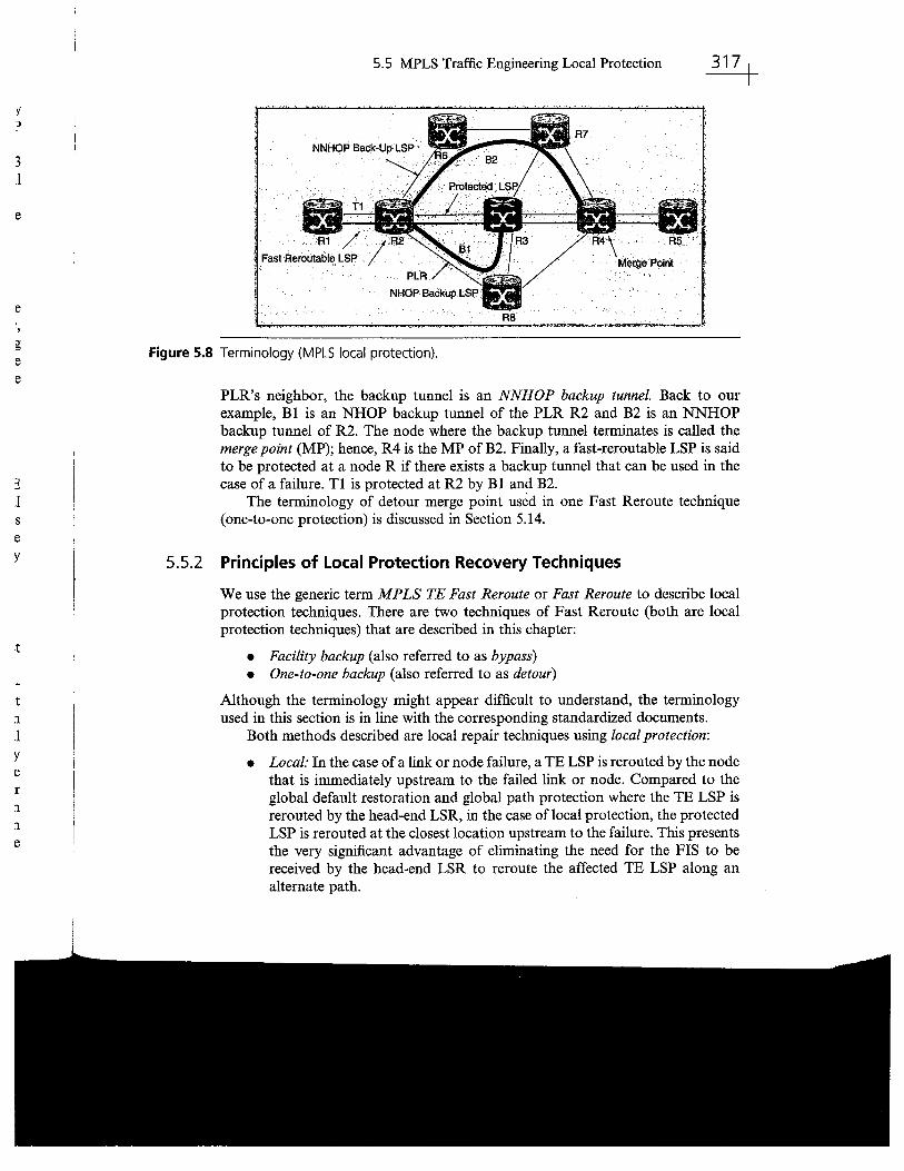
As depicted in Figure 5.9, with one-to-one backup, at each hop, one backup LSP(called a Detour LSP) is created for each fast-reroutable TE LSP. So, for instance,at the node R3, to protect the set of fast-reroutable TE LSPs Tl, T2, and T3, thefollowing set of backup TE LSPs are set up:
. One Detour LSP DI for the protected TE LSP Tl, following the pathR3-RIO-RI1-R5-R6
Figure 5.9 Illustration of the Detour LSP with one-to-one backup.
-... -~. ~,,-, .-- '-." .._-"
Fi
5.5 MPLS Traffc Engineering Local Protection ~. One Detour LSP D2 for the protected TE LSP T2, following the path
R3-R8-R5-R9. One Detour LSP D3 for the protected TE LSP T3, following the path
R3-RIO-RI1-RI2
Note that this only protects the fast-reroutable TE LSPs Tl, T2, and T3 against afailure of the link R3-R4 and the node R4. Similarly, each node along the fast-reroutable TE LSP paths wil perform the same operation.
At each PLR along the fast-reroutable TE LSP path, a local backup tunnelcalled Detour LSP that avoids the protected resource and terminates on the tail-endLSR for the fast-reroutable TE LSP is set up. In the previous example, for thefast-reroutable TE LSP Tl, R3 sets up a Detour LSP DI originated at R3 andterminated at R6 that avoids both the link R3-R4 and the node R4.
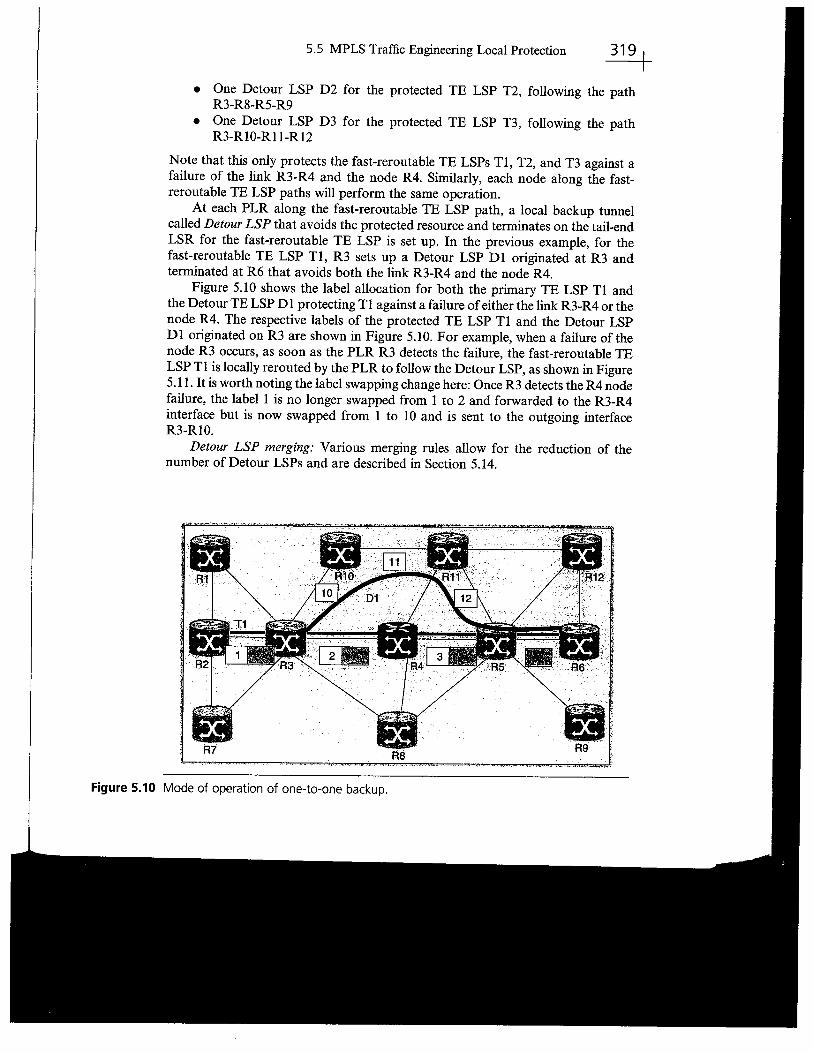
Figure 5.10 shows the label allocation for both the primary TE LSP Tl andthe Detour TE LSP D 1 protecting Tl against a failure of either the link R3- R4 or thenode R4. The respective labels of the protected TE LSP Tl and the Detour LSPDI originated on R3 are shown in Figure 5.10. For example, when a failure of thenode R3 occurs, as soon as the PLR R3 detects the failure, the fast-reroutable TELSP Tl is locally rerouted by the PLR to follow the Detour LSP, as shown in Figure5.11. It is worth noting the label swapping change here: Once R3 detects the R4 nodefailure, the label i is no longer swapped from 1 to 2 and forwarded to the R3-R4interface but is now swapped from i to 10 and is sent to the outgoing interfaceR3-RIO.
Detour LSP merging: Various merging rules allow for the reduction of thenumber of Detour LSPs and are described in Section 5.14.
RS.""~~ -~-...~"...- ~ - ,.- ~ ~ ,,~
Figure 5.10 Mode of operation of one-to-one backup.

~5.5.4
CHAPTER 5 MPLS Traffic Engineering Recovery Mechanisms
Local Protection: "Facility Backup"
By contrast with one-to-one backup, with facility backup, just one backup tunnel perNHOP is required to protect against a link failure and one NNHOP backup tunnel isrequired to protect against a node failure. Of course, an NNHOP protects against notonly a node failure (the bypassed node) but also the link between the immediatelyupstream node and the bypassed node. As discussed later, there are some benefits insetting up both NHOP and NNHOP backup tunnels. More accurately, a small set ofbackup tunnels may be required if bandwidth protection must be guaranteed (seeSection 5.15 for more details on bandwidth protection), but the key point is that thenumber of required backup tunnels is not a function of the number ofTE LSPs in theMPLS network, which is a crucial property to preserve scalability.
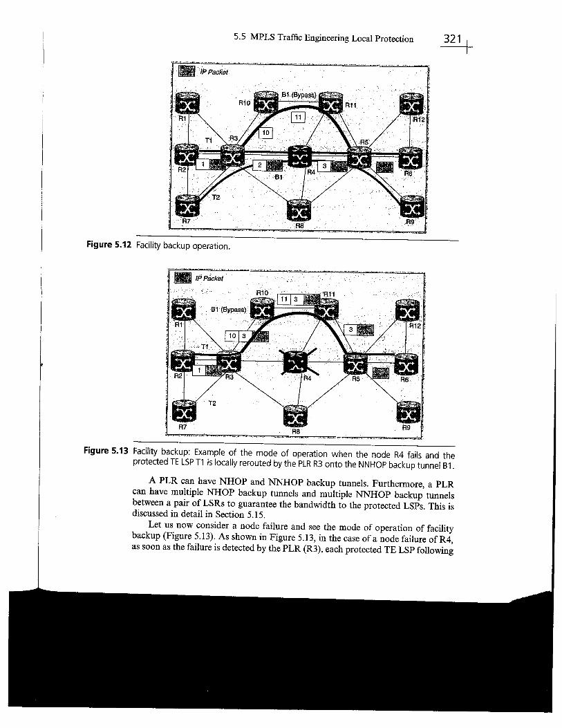
In Figure 5.12, a single NNHOP backup tunnel (bypass) is confgured on R3(PLR) to protect any fast reroutable TE LSP traversing the node R3 and followigthe R3-R4-R5 path against a failure of the link R3-R4 or the node R4 (indeed, thesame NNHOP backup tunnel can be used in both failure scenarios). R5 is the mergepoint. Hence, for instance, the two fast-reroutable TE LSPs Tl and T2 are pro-tected by the NNHOP bypass tunnel Bl that follows the path R3-RIO-Rll-R5.
Let us now consider a fast-reroutable TE LSP T1 that follows the path R2-R3-R4-R5-R6. As shown in Figue 5.12, the corresponding labels are distributed inRSVP Resv messages (R5 distributes the label "3" to R4, R4 distributes the label "2"to R3, R3 distributes the label "i" to R2). In this example, a bypass tunnel Bl
starting at the PLR R3 is also set up to protect against a link failure of
the link R3-R4and a node failure ofR4. The corresponding labels are depicted in Figure 5.12.
Note: In the case of an NHOP backup tunnel, this is often referred to as MPLS TEFast Reroute link protection. When the backup tunnel is an NNHOP backup tunnel,this is usually called MPLS TE Fast Reroute node protection.
Figure 5.11 One-to-one backup: Example of the mode of operation when the node R4 fails and theprotected TE LSP Tl is locally rerouted by the PLR R3 onto its Detour LSP Dl.
5.5 MPLS Traffc Engineering Local Protection B4-, ."~ - ,._. .~. - .-
~ i- LP Packet
,,"._- -..".,'...., --,. -~---.,-' ~ '.
Figure 5.12 Facility backup operation.
Figure 5.13 Facility backup: Example of the mode of operation when the node R4 fails and theprotected TE LSP Tl is locally rerouted by the PLR R3 onto the NNHOP backup tunnel 81.
A PLR can have NHOP and NNHOP backup tunnels. Furthermore, a PLRcan have multiple NHOP backup tunnels and multiple NNHOP backup tunnelsbetween a pair of LSRs to guarantee the bandwidth to the protected LSPs. This isdiscussed in detail in Section 5.15.
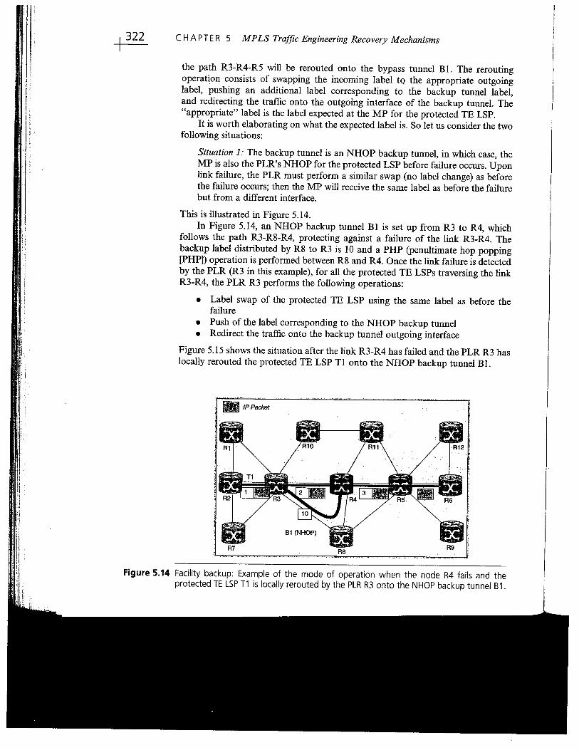
Let us now consider a node failure and see the mode of operation of facilitybackup (Figure 5.13). As shown in Figure 5.13, in the case of a node failure of R4,as soon as the failure is detected by the PLR (R3), each protected TE LSP following
, ~.- - ~ ~
~ CHAPTER 5 MPLS Traffc Engineering Recovery Mechanisms
i ;
II. i .
the path R3-R4-R5 wil be rerouted onto the bypass tunnel Bl. The reroutingoperation consists of swapping the incoming label tQ the appropriate outgoinglabel, pushing an additional label corresponding to the backup tunnel label,and redirecting the traffc onto the outgoing interface of the backup tunnel. The"appropriate" label is the label expected at the MP for the protected TE LSP.
It is worth elaborating on what the expected label is. So let us consider the twofollowing situations:
Situation 1: The backup tunnel is an NHOP backup tunnel, in which case, theMP is also the PLR's NHOP for the protected LSP before failure occurs. Uponlink failure, the PLR must perform a similar swap (no label change) as beforethe failure occurs; then the MP will receive the same label as before the failurebut from a different interface.
This is ilustrated in Figure 5.14.
In Figure 5.14, an NHOP backup tunnel BI is set up from R3 to R4, whichfollows the path R3-R8-R4, protecting against a failure of the link R3-R4. Thebackup label distributed by R8 to R3 is 10 and a PHP (penultimate hop popping(PHP)) operation is performed between R8 and R4. Once the link failure is detectedby the PLR (R3 in this example), for all the protected TE LSPs traversing the linkR3-R4, the PLR R3 performs the following operations:
. Label swap of the protected TE LSP using the same label as before the
failure. Push of the label corresponding to the NHOP backup tunnel. Redirect the traffc onto the backup tunnel outgoing interface
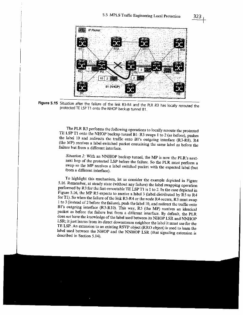
Figure 5.15 shows the situation after the link R3-R4 has failed and the PLR R3 haslocally rerouted the protected TE LSP T1 onto the NHOP backup tunnel Bl.
.. /P Packet
. .'-"--,- -,
Figure 5.14 Facility backup: Example of the mode of operation when the node R4 fails and theprotected TE LSP Tl is locally rerouted by the PLR R3 onto the NHOP backup tunnel Bl.
5.5 MPLS Traffc Engineerig Local Protection 4
Figure 5.15 Situation after the failure of the link R3-R4 and the PLR R3 has locally rerouted the
protected TE LSP Tl onto the NHOP backup tunnel B 1.
., ,-,,-- - .,'
The PLR R3 performs the following operations to locally reroute the protectedTE LSP Tl onto the NHOP backup tunnel Bl: R3 swaps i to 2 (as before), pushesthe label 10 and redirects the traffc onto Bl's outgoing interface (R3-R8). R4(the MP) receives a label-switched packet containing the same label as before thefailure but from a different interface.
Situation 2: With an NNHOP backup tunnel, the MP is now the PLR's next-next hop of the protected LSP before the failure. So the PLR must perform aswap so the MP receives a label switched packet with the expected label (butfrom a different interface).
To highlight this mechanism, let us consider the example depicted in Figure5.16. Remember, at steady state (without any failure) the label swapping operationperformed by R3 for the fast-reroutable TE LSP Tl is 1 to 2. In the case depicted inFigure 5.16, the MP R5 expects to receive a label 3 (label distributed by R5 to R4for Tl). So when the failure of the link R3-R4 or the node R4 occurs, R3 must swapi to 3 (instead of 2 before the failure), push the label 1 0, and redirect the traffc ontoBI's outgoing interface (R3-RlO). This way, R5 (the MP) receives an identicalpacket as before the failure but from a different interface. By default, the PLRdoes not have the knowledge of the label used between its NHOP LSR and NNHOPLSR; it just learns from its direct downstream neighbor the label it must use for theTE LSP. An extension to an existing RSVP object (RRO object) is used to learn thelabel used between the NHOP and the NNHOP LSR (that signaling extension isdescribed in Section 5.14).

~ CHAPTER 5 MPLS Traffc Engineering Recovery Mechanisms
- . '", "'",': .-~-..~. ~."" .p..4 .
. ~ IP Packet~ -'''"-O"",!,,,,'-,''C-...n..,..-". _. .'. ,~, ,,c-. -,..""4'~' . -'-"", ",.
B1 (Bypass) IIY "12
R7
103 J
~r/~II R9R8--,'" ,,-..~.., ~, -,. - , ., "'- - -" ,~_. ..-.,.-" v --~ ~'.. _. -. '~,,--,-.,
Figure 5.16 Situation after the failure of the link R3-R4 and the PLR R3 has locally rerouted theprotected TE LSP Tl onto the NNHOP backup tunnel B 1.
~ Important notes:
Note 1: An identical operation is performed for every protected LSP reroutedonto the same backup tunnel; indeed, with facility backup, the same backupLSP is used for all the rerouted TE LSPs that intersect the backup tunnel onboth the PLR and the MP.
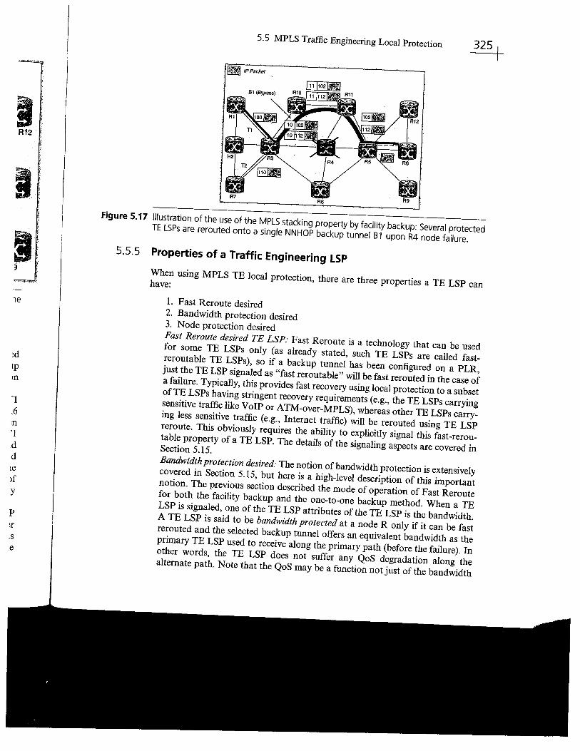
This is illustrated in Figure 5.17. This figure shows two primary tunnels T1and T2 that used to follow the paths RI-R3-R4-R5-R6 and R7-R3-R4-R5-R6before the failure. The labels in use are 100 (between Rl and R3), 101 (betweenR3 and R4), 102 (between R4 and R5) and PHP (between R5 and R6) for T1and 110 (between R7 and R3), ILL (between R3 and R4), 112 (between R4 andR5) and PHP between R5 and R6. Because both T1 and T2 intersect at R3 andR5, the same NNHOP backup tunnel Bl can be used in the case offailure of
thelink R3-R4 or node R4. This is of course a very important scaling property offacility backup that uses MPLS stacking. Note also that the same propertyapplies to NHOP backup tunnels.Note 2: In both cases (NHOP and NHOP bypass tunnels), no additional RSVPstates are created along the backup paths for the rerouted TE LSPs. In otherwords, the LSRs along the backup path do not "see" the rerouted TE LSPs asfar as the control plane is concerned. This is also a crucial property for thescalability properties of this solution.
5.5 MPLS Traffc Engineering Local Protection ql- IP Packet ~
IR12
II
Figure 5.17 Illustration of the use of the MPLS stacking property by facility backup: Several protectedTE LSPs are rerouted onto a single NNHOP backup tunnel B 1 upon R4 node failure.
5.55 Properties of a Traffic Engineering LSP;)
When using MPLS TE local protection, there are three properties a TE LSP canhave:
1. Fast Reroute desired
2. Bandwidth protection desired3. Node protection desiredFast Reroute desired TE LSP: Fast Reroute is a technology that can be usedfor some TE LSPs only (as already stated, such TE LSPs are called fast-reroutable TE LSPs), so if a backup tunnel has been confgured on a PLR,just the TE LSP signaled as "fast reroutable" wil be fast rerouted in the case ofa failure. Typically, this provides fast recovery using local protection to a subsetofTE LSPs having stringent recovery requirements (e.g., the TE LSPs carryingsensitive traffc like VoIP or ATM-over-MPLS), whereas other TE LSPs carry-ing less sensitive traffc (e.g., Internet traffc) wil be rerouted using TE LSPreroute. This obviously requires the ability to explicitly signal this fast-rerou-table property of a TE LSP. The details of the signaling aspects are covered inSection 5.15.Bandwidth protection desired: The notion of bandwidth protection is extensivelycovered in Section 5.15, but here is a high-level description of this importantnotion. The previous section described the mode of operation of Fast Reroutefor both the facilty backup and the one-to-one backup method. When a TELSP is signaled, one of the TE LSP attributes of the TE LSP is the bandwidth.A TE LSP is said to be bandwidth protected at a node R only if it can be fastrerouted and the selected backup tunnel offers an equivalent bandwidth as theprimary TE LSP used to receive along the primary path (before the failure). Inother words, the TE LSP does not suffer any QoS degradation along thealternate path. Note that the QoS may be a function not just of the bandwidth
ie
~d
ipin
'1
.6
:n
'1
ddie
)f
y
pT;s
e
~ CHAPTER 5 MPLS Traffic Engineering Recovery Mechanisms
i
i
but also of the propagation delay or jitter. Section 5.15 details how backuppaths can be computed to provide such guarantees. When signaled, a protectedTE LSP can explicitly request bandwidth protection.Node protection desired: In some cases, also further discussed in Section 5.15, itmight not be possible for a PLR to fid both an NHOP and an NNHOPbackup tunnel offering full bandwidth protection. For example, let us considerthe simple case of three routers Rl, R2, and R3 connected in a row, and theRl-R2 link bandwidth is 20 Mbps and the R2-R3 link is 10 Mbps. Thenthe PLR may try to fid an NHOP backup tunnel with 20 Mbps worth ofbandwidth and an NNHOP backup tunnel with min(20,10) = 10 Mbps worthof bandwidth. Suppose that no such NNHOP backup tunnel can be found butjust an NNHOP backup tunnel of 5 Mbps. Then as new TE LSPs requesting forbandwidth protection are signaled, it may happen that no NNHOP backuptunnel offering bandwidth protection can be found. In this case, having anadditional signaled parameter explicitly requesting node protection is desirableand can be used as a tie break. So if the PLR has two requests for bandwidthprotection and cannot select an NNHOP backup tunnel for both of thembecause of insufficient bandwidth on the NNHOP backup tunnel, it can pref-erably select the NNHOP backup tunnel for the TE LSP having expresseda desire to get node protection in addition to bandwidth protection. Such aparameter has been standardized in (FAST-REROUTE) and is described inSection 5.15.
:j
H,1
it~ ':Il '.
~ ¡ :1
';.,
¡ ~.ij,
. ~ !
. ~ ;:''1J~, -j
II! i
I~ I
. 11
!iii
ili1'1:l i
Notion of Class of Recovery
The various TE LSP recovery requirements mentioned earlier allow an operatorto defie multiple CoRs and assign a different CoR to each TE LSP according toits recovery requirements. For instance, very sensitive traffic like voice-over-IP/MPLS or ATM-over-MPLS could be routed over protected TE LSPs withbandwidth and node protection. In the case of a link or node failure, those TELSPs would be very quickly rerouted, while maintaining an equivalent QoS. On theother hand, MPLS VPNs traffc could be routed onto protected TE LSPs withoutbandwidth protection. Finally the less sensitive traffc could be routed over non-protected TE LSPs.
Defining multiple classes of recovery provides the two following benefits:
. The set of rerouting operations can be prioritized. Indeed, every LSR
wil preferably start to recover the TE LSPs that belong to the highestCoR.
. When bandwidth protection is required, this implies reserving some backupcapacity in the network. With multiple CoRs, the amount of backupcapacity is limted to the set of TE LSPs that belong to the CoR forwhich bandwidth protection is required. This allows to signficantly opti-mie the required backup capacity.

5.5 MPLS Traffc Engineering Local Protection ~5.5.6 Notification of Tunnel Locally Repaired
As described earlier, upon detection of a link/node failure, the PLR imediatelystarts rerouting the set of protected TE LSPs over their respective backup tunnels(bypass tunnels or Detour LSPs). This may result in following a suboptimal end-to-end path. Consequently, in addition to performng the local reroute, the PLR sendsa specific RSVP Path Error message for each rerouted TE LSP to their respectivehead-end LSR to indicate that a local reroute has occurred. This type of RSVP PathError is sometimes qualifed as nondisruptive because no RSVP states are cleared; itserves as a pure indication to the head-end LSR. The receipt of such of message willthen trigger a reoptimization on the head-end LSR for the affected TE LSP. Indeed,as previously mentioned MPLS TE Fast Reroute is a temporary network recoverymechanism; the protected TE LSPs are quickly and locally rerouted onto backuptunnels using a local protection technique, but the path followed by the reroutedflows might no longer be optimaL. This is ilustrated in Figure 5.18.
In Figure 5.18, a protected TE LSP, Tl, following the path RO-RI-R2-R8 is setup. At router Rl (PLR), Tl is protected by an NHOP backup tunnel Bl againsta failure of the link RI-R2 (Bl follows the path Rl-R3-R4-R5-R2). When the linkRl-R2 fails, upon detecting the link failure, the PLR (Rl) reroutes the LSP Tlonto Bl and sends a Path Error "tunnel locally repaired" to TI's head-endLSR (RO). As you can see in Figure 5.18, the path followed by Tl is not optimal(RO-RI-R3-R4-R5-R2-R8). The receipt of the Path Error triggers a reoptimiationon RO, which in turn reroutes the TE LSP Tl along the path RO-R3-R4-R5-R2-R8,which is more optimal than the path followed by the rerouted flows during failure(RO-RI-R3-R4-R5-R2-R8). In this example, we assume that all the links have the
LSP1Path Once Rerouted
R6 R7 R8
Figure 5.18 Notification of local repair followed by head-end reoptimization,
~ CHAPTER 5 MPLS Traffc Engineering Recovery Mechanisms
same metric. Of course, the TE LSP reoptimization should always be performedusing the "make before break" procedure, avoiding any traffc disruption.
The head-end wil also be informed of the link failure via the receipt of an IGPupdate from one of the routers adjacent to the failed link. Either upon the receipt ofan RSVP Path Error notify message "tunnel locally repaired" or an IGP update,the head-end triggers a TE LSP reoptimization.
Case of a Multiarea (OSPF) or Multilevel (15-/5) Network
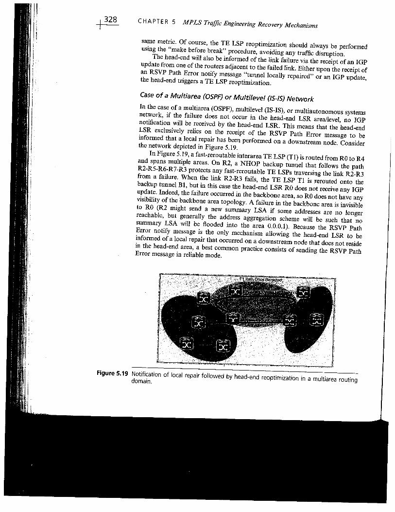
In the case of a multiarea (OSPF), multilevel (IS-IS), or multiautonomous systemsnetwork, if the failure does not Occur in the head-end LSR area/evel, no IGPnotification wil be received by the head-end LSR. This means that the head-endLSR exclusively relies on the receipt of the RSVP Path Error message to beinormed that a local repair has been performed on a downstream node. Considerthe network depicted in Figure 5.19.
In Figure 5.19, a fast-reroutable Interarea TE LSP (TI) is routed from RO to R4and spans multiple areas. On R2, a NHOP backup tunnel that follows the pathR2-R5-R6-R7-R3 protects any fast-reroutable TE LSPs traversing the link R2-R3from a failure. When the link R2-R3 fails, the TE LSP Tl is rerouted onto thebackup tunnel Bl, but in this case the head-end LSR RO does not receive any IGPupdate. Indeed, the failure occurred in the backbone area, so RO does not have anyvisibility of the backbone area topology. A failure in the backbone area is invisibleto RO (R2 might send a new sumary LSA if some addresses are no longerreachable, but generally the address aggregation scheme will be such that nosumary LSA will be flooded into the area 0.0.0.1). Because the RSVP PathError notify message is the only mechanism allowing the head-end LSR to beinformed of a local repair that occurred on a downstream node that does not residein the head-end area, a best common practice consists of sending the RSVP PathError message in reliable mode.
Figure 5.19 Notification of local repair followed by head-end reoptimization in a multiarea routingdomain.
5.5 MPLS Traffc Engineering Local Protection ~d 5.5.7
P,f3~,
Signaling Extensions for MPLS Traffic Engineering Local
Protection
IS
Pdie 5.5.8:r
4h3
ie
P
y.e
:r0hie
.e
h
By contrast with MPLS global default protection and MPLS TE global protection,which do not require any signaling protocol extensions beyond those of RSVP TEdefied in (RSVP-TEl for the signaling of MPLS TE LSP, MPLS TE loçal protec-tion (Fast Reroute) requires several signaling extensions. Although they areundoubtedly important, their detailed understanding is not a prerequisite to grasphow local protection works. Consequently, the signaling aspects of Fast Rerouteare covered in detail in Section 5.14.
Two Strategies for Deploying MPLS Traffic Engineering for FastRecovery
As mentioned in Section 5.1, there might be several motivations for deployingMPLS TE:
. Bandwidth optimization: So that the network resources are used in a more
effcient way. This also helps in providing better QoS.. Providing strict QoS guaranties to some specifc traffic flows.
. Fast recovery.
In some networks, there might be an interest in MPLS TE for its fast recoveryproperty only. In other words, bandwidth optimation and/or strict QoS guaran-tees are not required, but the operator would like to benefit from the fast recoveryproperty of Fast Reroute without tuning its IGP parameters as described in
Chapter 4. This section proposes two strategies for deploying MPLS TE when theonly objective is to get fast recovery by using Fast Reroute.
For instance, consider an underutilized (or overprovisioned) network. Such anetwork does not require any bandwidth optimation because it is not congested.Also, depending on the network load, QoS guarantees could rely on the simpleassumption that no link is congested and the link loads are very low. In such asituation, MPLS TE is not required, and paths computed by the routing protocolare perfectly satisfactory. However, such a network may require fast recovery oflink or node failures, making Fast Reroute a good candidate. Because Fast Rerouterequires TE LSPs, the solution includes deploying TE LSPs but in a quite specifcway, which we descabe in this section.
There are two strategies for deploying MPLS TE when the sole objective of theoperator is to use Fast Reroute:
i. With a full mesh of unconstrained TE LSPs2. With one-hop unconstrained TE LSPs
g
Network Design with a Full Mesh of Unconstrained TE LSPs
A simple and effcient strategy is to deploy a full mesh of unconstrained TELSPs. An unconstrained TE LSP is an LSP without any constraint. For instance,
~ CHAPTER 5 MPLS Traffc Engineering Recovery Mechanisms
the required bandwidth is 0, and no affnities are defined. The only property ofsuch a TE LSP is to be fast reroutable. Indeed, the objective is not to use thetraffc engineering property of MPLS TE (in the sense of "traffc engineer" theflows across the network). So the available bandwidth and other TE link-relatedinformation are stil flooded by the IGP TE extensions but will never change.
When a head-end LSR computes a path for an unconstrained TE LSP, thesame CSPF algorithm is used as with any other TE LSP, but the obviousoutcome is that the TE LSP wil follow the IGP shortest path. In other words,the traffc routed onto unconstrained TE LSPs wil follow the same paths asIP routed traffc, but in the case of link and/or node failures, fast-reroutableTE LSPs wil be rerouted by MPLS TE Fast Reroute, which was the initialobjective.
Network Design with Unconstrained One-Hop TE LSPs
If the requirement is to use Fast Reroute for link protection only, then exactly oneprimary unconstrained TE LSP plus one single NHOP backup tunnel are requiredfor every link to protect.
The idea is to set up a one-hop tunnel following the same path as the link toprotect. One way of achieving this is to set up an unconstrained TE LSP. This waythe CSPF algorithm wil just follow the most direct path between the head-end LSRand the tail-end LSR (the next hop of the head-end LSR in this case). Note that inthis case the PLR node is also the head-end LSR. Then the one hop primary TELSP must be confgured so that all the traffc follows the TE LSP.
It is important to note that because the TE LSP is a one-hop LSP, if PHP isused, no label is added once the traffic is routed over the priary TE LSP. Such astrategy is depicted in Figure 5.20.
In the example shown in Figure 5.20, the objective is to protect the link R2-R3.So a single-hop tunnel (Tl) is configured from R2 to R3 and all the traffic is routedonto this one-hop priary TE LSP through this link. Tl has no constraint, so thisTE LSP follows the path R2-R3. An NHOP backup tunnel BI is confguredbetween R2-R3 with the constraint of being diversely routed from the protectedlink and follows the path R2-R8-R3. As discussed in Section 5.15, additionalconstraints may be added to also provide bandwidth protection. In the case offailure of the link R2-R3, the PLR (R2) wil trigger Fast Reroute and all the trafficthat used to be routed over the lik R2-R3 wil be rerouted over Bl, following thepath R2-R8-R3. Then the priary TE LSP Tl wil be rerouted (reoptimed) and
wil follow the new shortest path between R2 and R3. Finally, the routing protocolwil be informed of the link failure and wil recompute a new path, which mayornot follow Bl's path.
The same configuration has to be repeated for each link to protect using FastReroute. Note that if the link R2-R3 is protected using a SONET/SDH protectedVCs, Fast Reroute may also be used to protect against a router interface failure onthe R2 or R3 side. In that case, one must ensure that both mechanisms are not
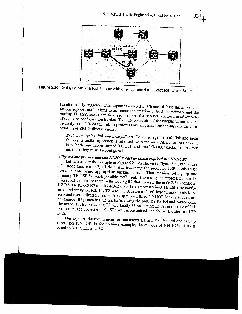
5.5 MPLS Traffc Engineering Local Protection ~
H8
Figure 5.20 Deploying MPLS TE Fast Reroute with one-hop tunnel to protect against link failure.
simultaneously triggered. This aspect is covered in Chapter 6. Existing implemen-tations support mechanisms to automate the creation of both the primary and thebackup TE LSP, because in this case their set of attributes is known in advance toalleviate the configuration burden. The only constraint of the backup tunnel is to bediversely routed from the link to protect (some implementations support the com-putation of SRLG-diverse paths).
Protection against link and node failures: To guard against both link and nodefailures, a similar approach is followed, with the only difference that at eachhop, both one unconstrained TE LSP and one NNHOP backup tunnel pernext-next hop must be confgured.
Why are one primary and one NNHOP backup tunnel required per NNHOP?Let us consider the example in Figure 5.21. As shown in Figure 5.21, in the case
of a node failure of R3, all the traffc traversing the protected LSR needs to bererouted onto some appropriate backup tunnels. That requires setting up onepriary TE LSP for each possible traffic path traversing the protected node. InFigure 5.21, there are three paths leaving R2 that traverse the node R3 to consider:R2-R3-R4, R2-R3-R 7 and R2-R3-R8. So three unconstrained TE LSPs are config-ured and set up on R2: Tl, T2, and T3. Because each of these tunnels needs to bererouted over a diversely routed backup tunnel, three NNHOP backup tunnels areconfgured: Bl protecting the traffc following the path R2-R3-R4 and routed ontothe tunnel Tl, B2 protecting T2, and fially B3 protecting T3. As in the case oflink
protection, the protected TE LSPs are unconstrained and follow the shortest IGPpath.
This explains the requirement for one unconstrained TE LSP and one backuptunnel per NNHOP. In the previous example, the number of NNOPs of R2 isequal to 3: R 7, R3, and R8.
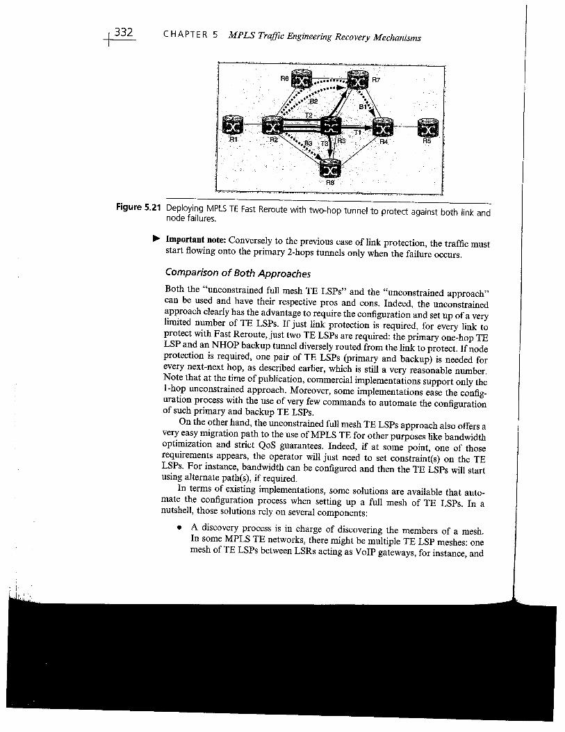
~ CHAPTER 5 MPLS Traffc Engineering Recovery Mechanisms
Figure 5.21 Deploying MPLS TE Fast Reroute with two-hop tunnel to protect against both link andnode failures.
~ Important note: Conversely to the previous case of link protection, the traffic muststart flowing onto the primary 2-hops tunnels only when the failure occurs.
Comparison of Both Approaches
Both the "unconstrained full mesh TE LSPs" and the "unconstrained approach"can be used and have their respective pros and cons. Indeed, the unconstrainedapproach clearly has the advantage to require the configuration and set up of a verylimited number of TE LSPs. If just link protection is required, for every link toprotect with Fast Reroute, just two TE LSPs are required: the primary one-hop TELSP and an NHOP backup tunnel diversely routed from the link to protect. Ifnodeprotection is required, one pair of TE LSPs (primary and backup) is needed forevery next-next hop, as described earlier, which is stil a very reasonable number.Note that at the time of publication, commercial implementations support only thel-hop unconstrained approach. Moreover, some implementations ease the config-uration process with the use of very few commands to automate the confguationof such primary and backup TE LSPs.
On the other hand, the unconstrained full mesh TE LSPs approach also offers avery easy migration path to the use of MPLS TE for other purposes like bandwidthoptimation and strict QoS guarantees. Indeed, if at some point, one of thoserequirements appears, the operator wil just need to set constraint(s) on the TELSPs. For instance, bandwidth can be configured and then the TE LSPs wil startusing alternate path(s), if required.
In terms of existing implementations, some solutions are available that auto-mate the configuration process when setting up a full mesh of TE LSPs. In anutshell, those solutions rely on several components:
. A discovery process is in charge of discovering the members of a mesh.In some MPLS TE networks, there might be multiple TE LSP meshes: onemesh ofTE LSPs between LSRs acting as VoIP gateways, for instance, and
5.6 Another MPLS Traffc Engineering Recovery Alternative ~another full mesh of TE LSPs between routers carrying the Internet traffic.Each TE mesh has its own set of characteristics in terms of bandwidth,priority, and protection/restoration, to mention just a few requirements.Then each router uses an IGP extension (OSPF or IS-IS) to advertise that itis a member of one or multiple TE meshes. This mechanism allows everyrouter to discover all the other routers that belong to the same TE mesh.
. Then, once a router has discovered all the routers that belong to the same
mesh, it can use a "template" (where the constraints specific to that par-ticular mesh are locally specified) to set up the mesh of TE LSPs. Note thatin this particular context of using MPLS TE for fast recovery only, thetemplate is very restricted because the primary TE LSPs are unconstrained.
In terms of IGP, both methods are equivalent. The TE-related information isflooded by the IGP but wil never changed because the TE LSPs are unconstrainedand never reserve bandwidth.
5.6 Another MPLS Traffic Engineering Recovery Alternative
Another MPLS TE recovery alternative has been proposed but never got anytraction in the industry because of severe limitations: 1 + 1 packet protection
whose principle is to pennanently bridge the IP/MPLS traffic over two diverselyrouted TE LSPs. The traffc bridging is made on the head-end LSR, and thedecision to switch the traffic is performed by the tail-end LSR, which permanentlycompares the two identical received flows from the primary and secondary TELSPs. When a failure occurs in the network, the traffic received from one of theTE LSPs is affected. Once the tail-end LSR detects the failure, it switches to thesecondary TE LSP. Note that such a mechanism is also called a single-endedprotocol because the switching decision process is made by a single entity (the tail-end LSR in this case) without requiring any signaling exchange between the nodes.A failure may be a traffc interruption, an unaccptable error rate, or any other kindof defects. Once the tail-end LSR has performed the switch, it can either decide tostay indefinitely on this TE LSP and start using the other TE LSP (once restored) inthe case of failure of the currently selected TE LSP or decide to switch back to theoriginal TE LSP, once restored.
Although this mechanism is simple and effcient in terms of recovery time, it hastwo major drawbacks that drastically limit its applicability:
. The amount of traffic forwarded in the network is doubled for each TE LSPprotected with this 1 + 1 mechanism. This is a serious issue because itbasically implies at least66 a bandwidth wastage of 50%.
66This technique implies at least a bandwidth wastage of 50% because one of the constraints of the
backup TE LSP is to be disjoint from the protected TE LSP, which usually means that it will follow alonger path.
~ CHAPTER 5 MPLS Traffc Engineering Recovery Mechanisms
. The failure discovery at the tail-end LSR usually requires some hardware
changes and thus equipment replacement, which can also be expensive.
For those reasons, such a mechanism has never been implemented or deployed butis just mentioned here for the sake of completeness in describing MPLS TE recoverytechniques.
5.7 Load Balancing
Load balancing is a technique to forward the traffc from a source to a destinationacross multiple paths. With equal load balancing, the traffc is balanced across
multiple equal-cost paths. lOP, like OSPF or IS-iS, pedorms equal
load balancing.This can be done on a per-packet basis (packets are sent along N equal-cost pathsusing a round-robin algorithm) or via some more sophisticated technques avoidingpacket reordering described in Chapter 4. With MPLS TE, both equal and unequalload balancing are supported. For instance, if there are two TE LSPs, Tl and T2between two LSRs, LSRl and LSR2, with respective bandwidth Bwl and Bw2,then LSRl can decide to balance the traffc whose destination is LSR2 (or beyond)in proportion to the respetive bandwidths Bwl and Bw2. Usually load balancing inMPLS TE-enabled networks is used when a single path obeying the set of con-straints cannot be found between two LSRs. For instance, a TE LSP of B Mbps isrequired and no path with the required amount of bandwidth is available. Then thesolution is to set up N LSPs so the sum of their bandwidth is equal to B. Anotherconstraint can be added when the path computation of the set of N LSPs isperformed like path diversity (the set of network elements traversed by the TELSPs are disjoint).
Strctly speakig, load balancing is not an MPLS TE recovery technque, so whydedicate a section to it?
Because a positive side effect of load balancing is that when the flow between twopoints is balanced across multiple paths, the probabilty of simultaneous failures ofall those paths is reduced compared to a single path, especially if those paths areexplicitly diversely routed. Hence, the overall availability is increased. Ths propertyhas been used by some operators to reduce the impact of network failure on specificflows.
Let us ilustrate that statement through the example in Figure 5.22. In this case,strictly speaking, the network availability is not increased but the impact of anetwork element failure on the traffc flows between two points is reduced.
In Figure 5.22, the two POPs of Sevila and Barcelona are made of two VoIPgateways and one LSR connected to the core of the network. The VoIP traffc iscarred onto TE LSPs. In this case, even if all the traffc between LSR i and LSR2could be carried onto a single TE LSP, two diversely routed TE LSPs are estab-lished between LSRl and LSR2 (with the same bandwidth or different bandwidths)and the traffc is balanced onto those two TE LSPs. In the case of a network failure,
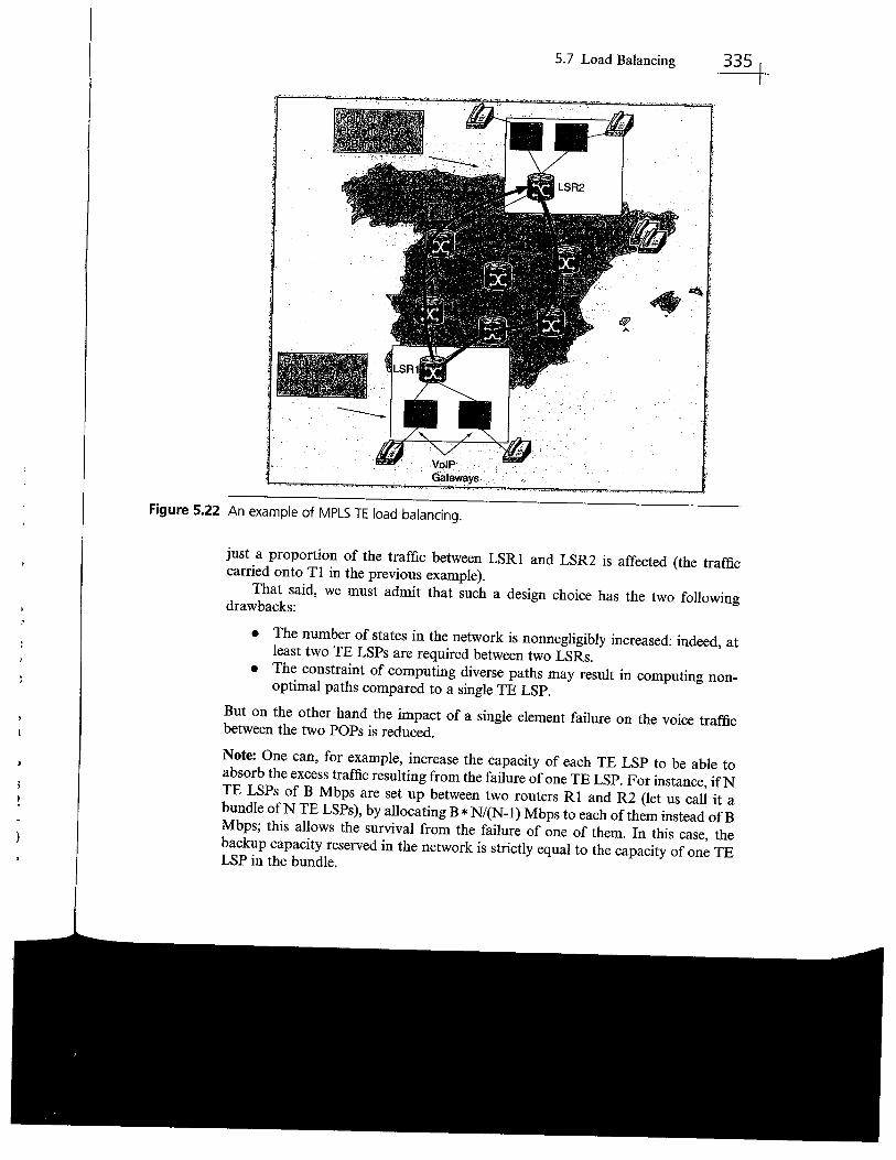
5.7 Load Balancing ~
Figure 5.22 An example of MPLS TE load balancing.
'. '" '
~....l!"
- -~. -'."- -- .- ,_. .- ,'. - ~ . - -
just a proportion of the traffic between LSRI and LSR2 is affected (the trafficcarred onto TI in the previous example).
That said, we must admit that such a design choice has the two followingdrawbacks:
. The number of states in the network is nonnegligibly increased: indeed, atleast two TE LSPs are required between two LSRs.
. The constraint of computing diverse paths may result in computing non-
optimal paths compared to a single TE LSP.
But on the other hand the impact of a single element failure on the voice traffcbetween the two POPs is reduced.
Note: One can, for example, increase the capacity of each TE LSP to be able toabsorb the excess traffc resulting from the failure of one TE LSP. For instance, ifNTE LSPs of B Mbps are set up between two routers Rl and R2 (let us call it abundle ofN TE LSPs), by allocating B * N/(N-l) Mbps to each of them instead ofBMbps; this allows the survival from the failure of one of them. In this case, thebackup capacity reserved in the network is strictly equal to the capacity of one TELSP in the bundle.
e CHAPTER 5 MPLS Traffc Engineering Recovery Mechanisms
5.8 Comparison of Global and Local Protection
As previously described in Chapter 1, the evaluation of a recovery mechanismrequires the consideration of several parameters: scope of recovery (link, node,SRLG), recovery time, guaranteed bandwidth, backup capacity requirements, stateoverhead, scalability, reordering, additive latency and jitter, signaling requirements,stability, and others. Throughout this chapter, we saw several MPLS TE recoverytechnques, so the natural question that comes to mind is, which one to use. Althoughthere is no unique answer because each network has its own constraint and require-ments, the aim of this section is to provide a comparisòn of the global protection andlocal protection technques with a particular focus on three key performance aspects:
. The recovery time
. The state overhead, which is directly correlated to the scalability
. The abilty to perform bandwidth sharing when bandwidth protection is
required
5.8.1 Recovery Time
With global protection, rerouting is performed by the head-end LSR, which meansthat this requires for the head-end LSR to receive the failure notifcation to reroute theaffected traffc onto their respective backup paths (whose paths have been precom-puted and signaled). So in terms of recovery time, the delta between global and localprotection is the failure indication signal propagation time to the head-end LSR. Howlarge this delta is higWy depends on the network characteristics. Thus, for instance,a network confed to a small country generally implies short propagation delays(less than 10 ms); on the other hand, an international network may easily experiencemuch longer propagation delays. . . up to a few hundreds of milliseconds. In thatcase, convergence of a few tens of miiseconds requires the use of local protectiontechniques. Furthermore, queuing delays to process the control plane notification(RSVP and/or IGP) messages can be reduced via the use ofQoS mechanisms.
Note that in terms of recovery time, the two local protection schemes describedearlier (i.e., "one-to-one" and "facility backup") are equivalent; they both rely onlocal protection where fast-reroutable TE LSPs are locally rerouted on presignaledbackup tunnels and then reoptirned by their respective head-end LSR.
In sumary, as far as the recovery time is concerned, the key diference betweenlocal and global protection is in the failure propagation notification time to the head-end LSR which, in the case of global protection is made of incompressible propaga-tion delays and queuing delays that can be reduced by means of QoS mechanisms.
5.8.2 Scalabilty
Scalabilty is undoubtedly one of the major aspects to consider when evaluating arecovery mechanism, and to that respect, global path protection, one-to-onebackup, and facility backup local protection differ very signifcantly.
5.8 Comparison of Global and Local Protection lEScalability is a relatively generic term that requires clarication in this context.
Protection mechanisms require setting up backup tunnels before any failure toprovide fast convergence (by contrast with global default restoration, the backuppath is already computed and signaled). The confguration of backup tunnels can befacilitated via an automatic process, but setting up backup tunnels in a network isnot entirely cost free. Although the scalability of RSVP is very high, in largenetworks, the number of backup tunnels can be signcant as shown below,
which requires to potentially handle a large number of states on routers. Moreover,the troubleshooting task is even more complicated for the team in charge ofoperating the network. So scalabilty is considered in terms of number of requiredbackup tunnels in this context.
Let us evaluate the number of required backup tunnels with global pathprotection, Fast Reroute facility backup, and one-to-one, based on the followingassumptions:
D: network diameter (average number of hops between a head-end LSR and atail-end LSR)C: degree of connectivity (average number of
neighbors)L: total number of links to be protected with Fast Reroute67N: total number of nodes (LSRs)T: total number of protected TE LSPs in the MPLS networkBu: number of backup tunels requiredK number of class of recovery (as mentioned in Section 5.5.5, there might beseveral classes ofTE LSPs, each requirig different CoR. In this case, each CoRhas a dedicated set of backup tunnels)S: average number of splits (as discussed in Section 5.15, in some cases wherebandwidth protection is required and backup bandwidth is a very scarceresource, more than one backup tunnel per protected link/node may berequied if a single backup tunnel with enough bandwidth cannot be found)
Note: Realistic assumptions for Sand K are as follows:
. S.: 4: Generally S wil very rarely exceed 3. In a network where bandwidth
protection is required but backup capacity is not a very scarce resource S = 1.If bandwidth protection is not required, then S = 1.
. Also K .: 3.
M: number of meshes in the network (e.g., there may be multiple meshes ofTELSPs in a network serving diferent pUrposes: one mesh for the voice traffc andone mesh for the data traffc).
It follows that
-. L .: N * C (because some links may not be protected by Fast Reroute)
-. T = M * N * (N-1) (assuming a full mesh TE deployment)
67Some links may be protected via other means like SONET/SDH and optical protection/restoration.