moving beyond simple examples: assessing the …llobet/multidim2.pdfmoving beyond simple examples:...
TRANSCRIPT

Moving Beyond Simple Examples: Assessing theIncremental Value Rule within Standards∗
Anne Layne-FarrarCharles River Associates
Gerard LlobetCEMFI
July 26, 2013
Abstract
This paper presents a model of patent licensing in a standard setting contextwhen patented technologies are heterogeneous in multiple dimensions. The modelallows us to assess a policy proposal put forth in the literature: that an incre-mental value pricing rule should define Fair, Reasonable, and Non-Discriminatory(FRAND) patent licensing within standard setting organizations as it replicates theex ante efficient competition outcome. We find that when patented technologiesmust be weighed on numerous factors, and not simply one-dimensional cost-savings,there is unlikely to be a single incremental value that can be agreed upon by allrelevant parties. Furthermore, ex ante competition fails to select the efficient tech-nologies by penalizing the more versatile ones. These results cast some doubt onthe usefulness of the incremental value as a precise benchmark for FRAND.
JEL codes: L15, L24, O31, O34.keywords: Intellectual Property, Standard Setting Organizations, FRAND, Patent Li-censing, Incremental Value.
∗We benefited from comments by Guillermo Caruana and Andres Zambrano. We thank Qualcommfor financial support of the research behind this paper. We also thank Tim Simcoe, Marc Rysman, andan anonymous reviewer for their thoughtful suggestions. The ideas and opinions in this paper, as wellas any errors, are exclusively the authors’. Comments should be sent to [email protected] [email protected].
1

1 Introduction
Standard Setting Organizations (SSOs) are crucial in industries where different firms have
come to rely on product and service interoperability standards for their operations. Their
role is to coordinate the activities of a large variety of participants so that disparate and
competing firms can market products that all share a common platform or functionality.
From pure technology providers to final good producers to integrated players, firms that
participate in an SSO tend to have very different interests. Thus, one of the roles of
SSOs is to offer a forum for constructive cooperation, where otherwise competing firms
can work together to select technologies that will determine standards that can be broadly
implemented in products and services. One of the common SSO rules aimed at fostering
this constructive cooperation among a diverse membership is the request for firms that
believe they hold patents on the technologies selected for a standard to commit to license
(preferably at the time the standard is drafted) those patents to potential implementers
under Fair, Reasonable, and Non-Discriminatory (FRAND) terms.
Recent competition policy cases have brought attention to these licensing commit-
ments, which are commonly viewed as contracts between patent holding members and
the SSO (Brooks and Geradin, 2011). In the continuing search to bring greater clar-
ity and specificity to the concept of FRAND licensing within standard setting contexts,
economists have proposed – and policymakers have readily latched onto – the idea of
incremental value pricing. One early proposal to extend the idea of incremental value
pricing to patent licensing is found in the influential paper by Swanson and Baumol
(2005). This benchmark is based on the idea that after a technology has been selected as
part of the standardization effort and it becomes “essential” for the practice of a standard
(standard essential patents, or SEPs) its developer could gain market power through the
standardization process, which by definition eliminates alternatives. In order to coun-
2
teract this additional market power the SSO should aim to restore the ex-ante result.
That is, to replicate the result of a fictitious auction among competing technologies to be
selected, before standardization occurs. In that auction the licensing price would corre-
spond to the contribution to the commercial value that the selected technology engenders
over the best alternative.1 This ex post evaluation of the different technologies is con-
sistent with the incremental value rule used in other contexts (Farrell and Katz, 2005)
and it is the one that the FTC has in mind when calling upon courts to cap reasonable
royalty damages at “the incremental value of the patented invention over the next-best
alternative” (FTC, 2011). It defines incremental value in relation to the price that could
be commanded during the standard setting phase, assuming all R&D has been invested
and patents are in hand, with these existing technologies competing during standard
setting.
The question of how, exactly, to define “incremental value” is a pivotal one if the
proposals to base FRAND upon it are to move beyond mere proposals. Consider the case
of technologies that differ only in the cost of production. The cost differential between
two technologies translates ex-ante into a technology price that can be set through an
SSO auction, or any form of bargaining that takes place during standard setting, and
hence is able to capture competition among technologies. With a bit of detective work,
a one-dimensional cost-saving increment could also be used ex post (during a standard’s
commercialization), for capping reasonable royalties in any court or agency review of
disputed standard essential patents bound by FRAND commitments, as recommended in
the FTC (2011) IP Report. As long as the difference between two patented technologies
can be reduced to a single dollar amount, either production cost savings or increased
product price, this approach would provide a measure of incremental value.2
1They also argue that this price should incorporate costs like those associated with licensing or theongoing costs of R&D.
2This implementation abstracts from important aspects such as the incentives for firms to invest inR&D or participate in an SSO when they anticipate that their innovation will be licensed according to its
3
Unfortunately, in the context of SSOs, the interpretation of technology “quality” dif-
ferentials as one-dimensional dollar differences is unlikely to provide a framework rich
enough to analyze how an incremental-value rule could be implemented since the same
technology might mean different things to different potential licensees. The goal of this
paper is to understand how heterogeneity in the technologies that innovators may pro-
vide and the different valuation that their users may have affect the equilibrium licensing
agreements. Our model departs from the typical framework described above in two di-
rections. First, we consider technology quality in a broad sense, beyond one-dimensional
dollar differences as we make clear below. We evaluate the not-uncommon situation in
which different technologies imply different trade-offs among their characteristics for dif-
ferent SSO members. Technologies differ in their stand-alone value, understood in the
usual sense of raising the valuation of all consumers uniformly or reducing production
costs in a constant amount, and their versatility, understood as how suitable the technol-
ogy is for consumers that might use it for heterogeneous purposes. Second, we recognize
that neither SSO members nor the ultimate downstream consumers purchasing products
that implement standards is a monolithic group. Instead, different parties are likely to
place different “incremental values” on the same technology.
Our results show that, albeit intuitive, the much advertised properties of the incre-
mental value rule are not robust to considering innovations that are heterogeneous in
multiple dimensions. We show that incremental-value pricing loses the appealing prop-
erty of being just a function of technological differences. Instead, it becomes a function
of specific features of the industry such as the degree of heterogeneity of the uses of the
final product and the degree of competition in the final market. Furthermore, we show
that the ex-ante outcome, which is used as a justification for incremental value pricing,
incremental value. Indeed, Layne-Farrar et al. (2013) show that once these effects are considered incre-mental value pricing is inefficient even in this simple context since it discourages firms from participatingin the SSO.
4

is unlikely to be a good benchmark for the efficient arrangement that an SSO should aim
to achieve in the first place.
The two sources of heterogeneity we describe in our model are typical of most SSOs.
Interoperability standards cover complex products (computers, the internet, mobile phones)
whose contributing technologies typically cannot be evaluated solely on a one-dimensional
cost-savings basis. Instead, these technologies are more likely to compete on multiple di-
mensions, like transmission speed versus accuracy, software complexity versus hardware
cost, and so forth. Furthermore, the final users of the products created by firms that
make use of these technologies have heterogeneous preferences for the trade-offs that
these technologies entail.
An example of these multidimensional trade-offs is the debate in the early days of the
Wireless LAN standardization process, that gave rise to the current Wi-Fi technology.
In the late 1990s two different standardization efforts emerged. As Negus and Petrick
(2009) discuss, the OpenAir proposal emphasized interoperability between the offerings
of different providers intended for a variety of uses, from high-powered office deployments
to less demanding home uses. As such, this standard was highly versatile, though costly
in light of the high end applications it covered. The alternative HomeRF standardization
effort focused solely on the less-demanding home wireless LAN, and hence pursued low
costs by sharing components with cordless phones and targeting home users that valued
simplicity. Even within the SSO that pursued a versatile wireless solution capable of high
end needs, there were still important trade-offs to be made. One camp wanted robust
wireless that could be used indoors, meaning an emphasis on the so-called multipath
problem of signals bouncing off of solid surfaces and arriving at the destination out of
sync. Others within the SSO were more concerned with outdoor transmission, and hence
focused on transmission speeds.
Our model captures trade-offs of these sorts by considering a setup in which inno-
5
vators compete to sell their technology to downstream firms that use it to provide a
good in the final market. Downstream producers face heterogeneous consumers that may
choose between their products. Different technologies provide different value to the fi-
nal product but may also help in making the product appealing to a wider or narrower
set of consumers. We characterize the technology choice and the equilibrium royalties
that emerge under ex ante competition, the benchmark that the incremental value rule
is meant to replicate. As expected, when we focus on the value (or cost savings) di-
mension the model is analogous to that presented by Swanson and Baumol (2005) and
envisioned by the FTC (2011) IP Report. When we introduce the second dimension,
the versatility of the technology, we find that the notion of “incremental value” becomes
considerably more complicated. Abstracting from downstream competition we analyze
how the trade-offs between the characteristics that firms face change depending on the
characteristics of the market they serve, making the second dimension of the incremental
value (versatility/adaptability) market-specific.
Once we introduce competition, we characterize the equilibrium royalty that would
emerge under ex-ante competition among different technologies. Not very surprisingly,
this royalty takes into account not only the difference in stand-alone value among tech-
nologies, but also includes differences in their versatility. Interestingly, as opposed to
what a standard notion of the incremental value would suggest, the equilibrium royalty
price is lower for more versatile technologies, since they engender more competition in
the final market, reducing the willingness to pay of downstream producers. As a result,
technologies that are worse from a social point of view in both dimensions (lower value
and less versatility) and under a strict application of the incremental value rule would
command a lower royalty price would often be chosen.3 The previous results are robust
3The “excess of inertia” concept for the adoption of de facto standards, introduced in the literatureby Farrell and Saloner (1985) has similar implications. In that case users do not switch to a superiortechnology due to a lack of coordination. Here, however, firms may not adopt a better technology becausethey are afraid of the fiercer competition it might entail. In both cases, however, social welfare is reduced
6
to the existence of network effects as well as the possibility that firms adopt more than
one technology.
This paper contributes to the literature that analyzes the properties of the incremen-
tal value pricing. Farrell et al. (2007) supports the Swanson and Baumol (2005) logic,
proposing that a patent’s “incremental value” provides an upper bound (a cap) on the
licensing fees that patent owners participating in SSOs can obtain. Mariniello (2011) also
takes the incremental value concept as a key element in his proposed test for determin-
ing whether actual licensing rates assessed after the standard is set meet patent holders’
FRAND commitments, although he proposes that a patent’s “incremental value” pro-
vides a benchmark for ex post analysis and not a strict cap on allowable licensing rates.4
Neither Farrell et al. (2007) nor Mariniello (2011) provide a precise definition of “incre-
mental value” in relation to patented technology, but instead both rely more generally
on the notion of aggregate value added (such as cost savings in Farrell et al. (2007)).
Although less directly related, our work builds on the long literature on patent licens-
ing. Earlier models, summarized in Kamien (1992), study the optimal contract that a
monopolist may offer to various downstream competitors. More recent papers such as
Muto (1993) and Hernandez-Murillo and Llobet (2006) discuss the effect of the hetero-
geneity in the use that downstream firms can make of the innovation over the optimal
contract that the innovator offers. Schmidt (2009) and Rey and Salant (2012) also allow
for downstream heterogeneity and study the effect of licensing complementary patents on
the number of producers and competition in the final good market.
Although our paper does not model SSOs operations directly, it is also related to
the debate over the strategic behavior of firms in these organizations (Lerner and Tirole,
as a result.4Epstein et al. (2012) provide a qualitative discussion of a number of practical difficulties with an
incremental value cap, including the likelihood that different buyers will have different valuations fordifferent technologies, rendering the notion of a single incremental value over the next best alternativeunachievable.
7
2006) and how firms that contribute technology should be compensated in order to avoid
potential hold-up problems (Ganglmair et al., 2011).
Finally, we note the large literature on auctions that develops scoring rules in order to
express multi-dimensional attributes as single numbers. For example, Asker and Cantillon
(2008) develop a model in which suppliers submit offers on all dimensions of a good –
they consider price and the level of non-monetary attributes – where those offers are
evaluated using a scoring rule. While multiple dimensions can be reduced to a single one
using a scoring function, this reduction is only possible for attributes that can be rank
ordered, such as the “non-monetary” quality “levels” that Asker and Cantillon (2008)
consider. In the context of our model, however, the value that final good producers place
on the different dimensions of a technology depend on how they may affect downstream
competition. As a result, it might be the case that a technology that has higher quality
in both dimensions, and it is therefore more efficient, is not selected by downstream
producers. This feature rules out scoring functions as a criterion on which the incremental
value rule could be based.
The remainder of this paper proceeds as follows. In Section 2 we present the basic
model which the following sections build upon. In section 3, we develop the licensing
model for patented technologies that differ on at least two dimensions, where the down-
stream licensee is a monopolist. The model explicitly accounts for heterogeneity in the
uses of the technology and different firms face consumers with heterogeneous preferences
for multiple dimensions of the product. Section 4 introduces competition in the final mar-
ket. Section 5 adds network effects to better capture the cooperative standard-setting
environment. Section 6 concludes with a discussion of the policy implications of our
analysis.
8
2 The Basic Model
Consider a market where there are two upstream and two downstream firms. We denote
the upstream firms as innovators 1 and 2, and the downstream firms as producers A
and B. Downstream firms are competitors in a linear city of length one. Producer A is
located at 0 and producer B is located at 1. These downstream firms can sell products
that differ in two dimensions: the valuation that consumers assign to the good, v, and the
transportation cost of delivering the product to the consumer, α. As a result, a consumer
located at point x on the line facing prices pA and pB would obtain utility as follows:
U(x) =
{vA − αAx− pA if buying from A,vB − αB(1− x)− pB if buying from B.
We interpret v as the stand-alone “value” of the product and α as its “specificity.”5
We refer to technologies with a lower value of α as being more versatile, since this at-
tribute is related to how broad the market for the product is. We assume that consumers
are distributed according to the distribution function Φ(x). In most of the paper this
distribution will be assumed to be uniform between 0 and 1.
Upstream firms possess an innovation that downstream firms can embed in their final
products. For simplicity, we assume that the quality of the final good is determined
exclusively by this innovation, so that if upstream firm i = {1, 2} has an innovation with
attributes (vi, αi), this will also be the value of the product that the downstream producer
that licenses it will offer. We normalize the consumer valuation of a product when the
downstream firm does not adopt any of the innovations to 0.
Upstream innovators offer their technology at a per-unit royalty ri for i = 1, 2. Again
for simplicity, we assume that downstream producers have no marginal cost of production
aside from the royalty paid to the upstream innovator.
5Throughout the paper we will refer to (stand-alone) value as this vertical characteristic of the product.As it is usually the case, the results can be easily reinterpreted in terms of cost savings.
9

The timing of the model is as follows. In the first stage upstream innovators simulta-
neously choose the royalties that they offer to downstream producers. Downstream firms
then choose the innovation that maximizes their profits, anticipating the outcome that
will arise in the last stage of the game when they set their final prices, which is also done
simultaneously.
In order to analyze this model we will proceed in two steps. In the next section we
analyze the case in which there is only one downstream firm. This assumption allows us
to discuss how the choice of technologies changes with the level of heterogeneity among
consumers. In the following section we then discuss the equilibrium with multiple down-
stream firms, which allows us to assess the effects of competition. In section 5 we show
that results are qualitatively unchanged once we introduced network effects.
3 Downstream Monopolistic Producer
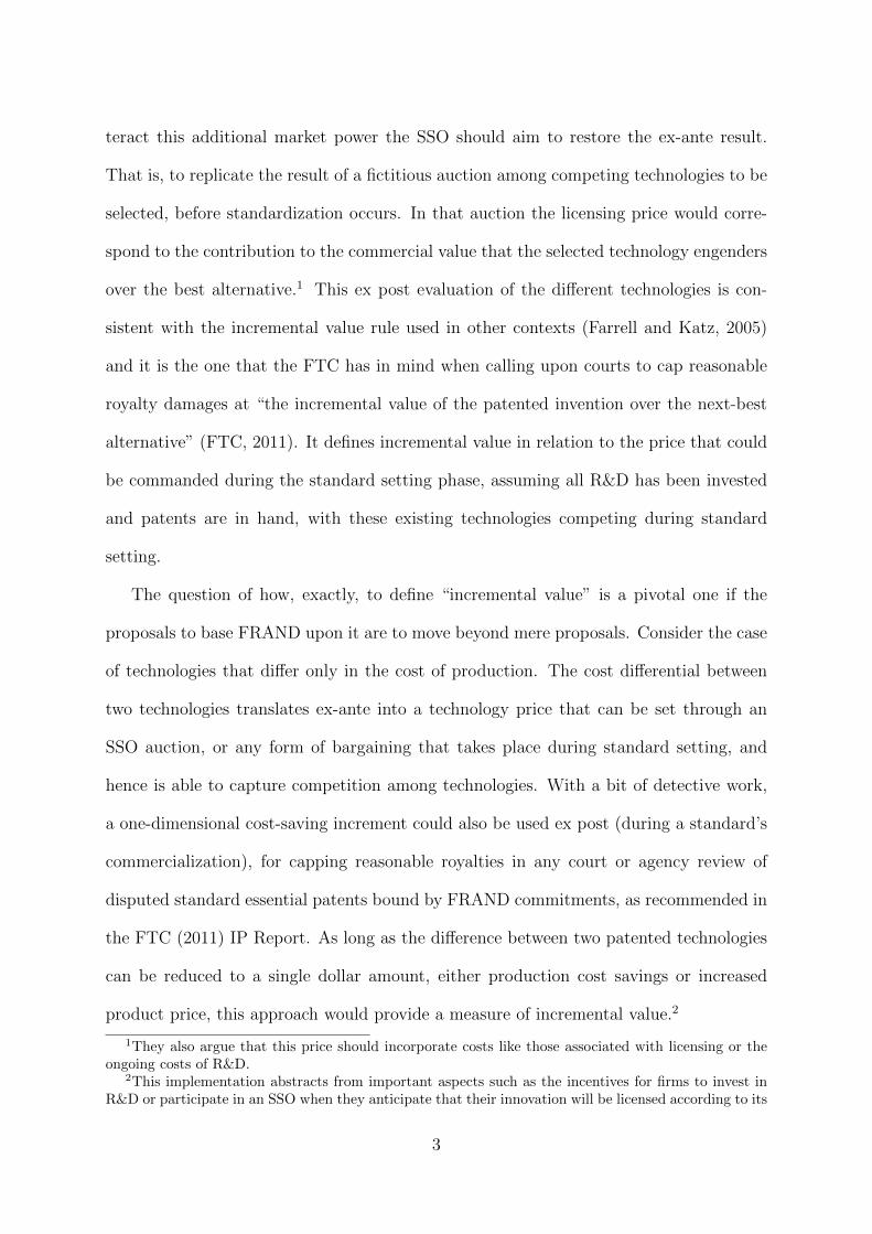
Consider the situation in which only firm A is present in the final market. In that case,
consumers will buy if their utility is positive. Let’s assume that the consumer location
x is distributed according to Φ(x) = xγ. The parameter γ ∈ [0, 1] can be interpreted as
a measure of how important heterogeneity among consumers is. In particular, if γ = 0
all consumers are homogeneous and their utility is v − p. As γ grows this heterogeneity
becomes more important. When γ = 1 consumers are uniformly distributed along the
unit line. The structure of the game is described in Figure 1.
In the second stage, if firm A obtains the technology from innovator i, demand arises
from consumers located at x ≤ x∗ ≡ vi−pAαi
, so that
DA(pA) = Φ
(vi − pAαi
)=
(vi − pAαi
)γ.
The previous demand is decreasing in the price and increasing in the value and versatility
10

I1 I2
A
0 1x∗
r1r2
pA
Figure 1: Structure of the game.
of the technology. This downstream producer will maximize profits according to
maxpA
(pA − ri)(vi − pAαi
)γ.
This expression leads to a monopoly price
p∗A = pM = max
{vi + γriγ + 1
, vi − αi}.
The first term arises in the interior solution, in which not all consumers buy. When
ri ≤ vi − 1+γγαi the royalty is sufficiently low so that the market is fully covered. In
order to simplify the exposition we rule out the corner solution by assuming that vi ≤ αi
so that in equilibrium not all consumers would buy even at a price 0. This assumption
implies that the versatility dimension is sufficiently important so that consumer decisions
are not driven entirely by the vertical dimension.
Under the previous assumption, profits from licensing the technology of firm i can, in
turn, be written as
ΠMA (i) =
(γ
αi
)γ (vi − ri1 + γ
)1+γ
.
As expected, profits for the downstream monopolist will be increasing in the versatility
of the technology (a low αi) and the stand-alone value vi.
11

In the first stage, given royalties r1 and r2 the downstream firm will choose the tech-
nology that leads to the highest profits. The following proposition characterizes the
equilibrium royalty rates that emerge as a result of the competition among innovators.
Proposition 1. Suppose that vi
αγ
1+γi
≥ vj
αγ
1+γj
. Then technology i will be adopted by the
downstream firm. The equilibrium royalties will be r∗j = 0 and
r∗i = vi −(αiαj
) γ1+γ
vj.
The technology chosen is efficient. That is, it coincides with the technology chosen in the
First Best.
The previous result emphasizes the fact that whether a technology is superior to the
other or not depends on its combination of attributes, both play a role. If a technology
is superior in both dimensions (i.e. a higher v and a lower α) that technology will be
adopted by any downstream monopolist. In many realistic situations, however, we expect
each technology to involve a trade-off between the two dimensions; one will have a higher
value and the other will be more versatile. Proposition 1 suggests that the resolution of
this trade-off, which determines the innovation that should command a positive royalty,
can be obtained by redefining the measure of value as vi
αγ
1+γi
.
The redefined expression for value, however, is endogenous to the characteristics of
the downstream buyer, through the parameter γ. An immediate consequence is that if
we consider different downstream monopolists that operate in different markets and face
different demands they will also have different preferences for the technologies. These
differences might be such that one manufacturer prefers technology 1 while the other
prefers technology 2. The reason is that differences in the parameter γ imply different
weights in the trade-off between the two technologies. In particular, if γ is high the
versatility becomes more important since consumers are more heterogeneous in their
12

tastes. Thus, a downstream firm that faces a higher value of γ will tend to choose the
more versatile technology.
Interestingly, that redefinition of value provides the right assessment about the tech-
nology that maximizes social welfare. So, even though market power downstream reduces
social welfare through higher prices, it does not bias the technology that the firm decides
to adopt. A proper benchmark for the optimal royalty should consider not only the
differences in this redefined valuation but also in the characteristics of the market that
licensees serve.6 A generalization of the ex-ante auctions proposed by Swanson and Bau-
mol (2005) using scoring auctions, for example, would implement the socially optimal
allocation. Of course, the weights in this auction should be market specific.
Trivially, standardization on a unique technology occurs in the case of a downstream
monopolist. In the rest of the paper we consider the situation in which there is down-
stream competition. In that case standardization will arise and become optimal when
network effects are large. For this reason, in the next section we consider the case in
which network effects are absent (or they are very weak) so that standardization might
not occur. In section 5 we discuss the opposite case in which strong network effects
are present resulting in standardization and a relevant role for SSOs in deciding among
different technologies.
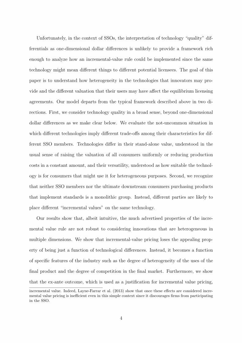
4 Downstream Competition
With the foundation laid in the simple downstream monopoly case, we now turn to the
case in which two producers, A and B, located at the two extremes of a linear city
compete in the final market. As in the previous case we will assume that innovator
6Of course, if both technologies have the same versatility the one with the highest value will beadopted. The resulting royalty for the “winning” firm will be r∗i = vi − vj , independent of the charac-teristics of the market. In other words, as the standard interpretation of the incremental value theoryindicates, if innovations differ only in the stand-alone value in equilibrium its creator will (and should inthis model) charge a royalty equal to the technology’s incremental value over the next best alternative.
13
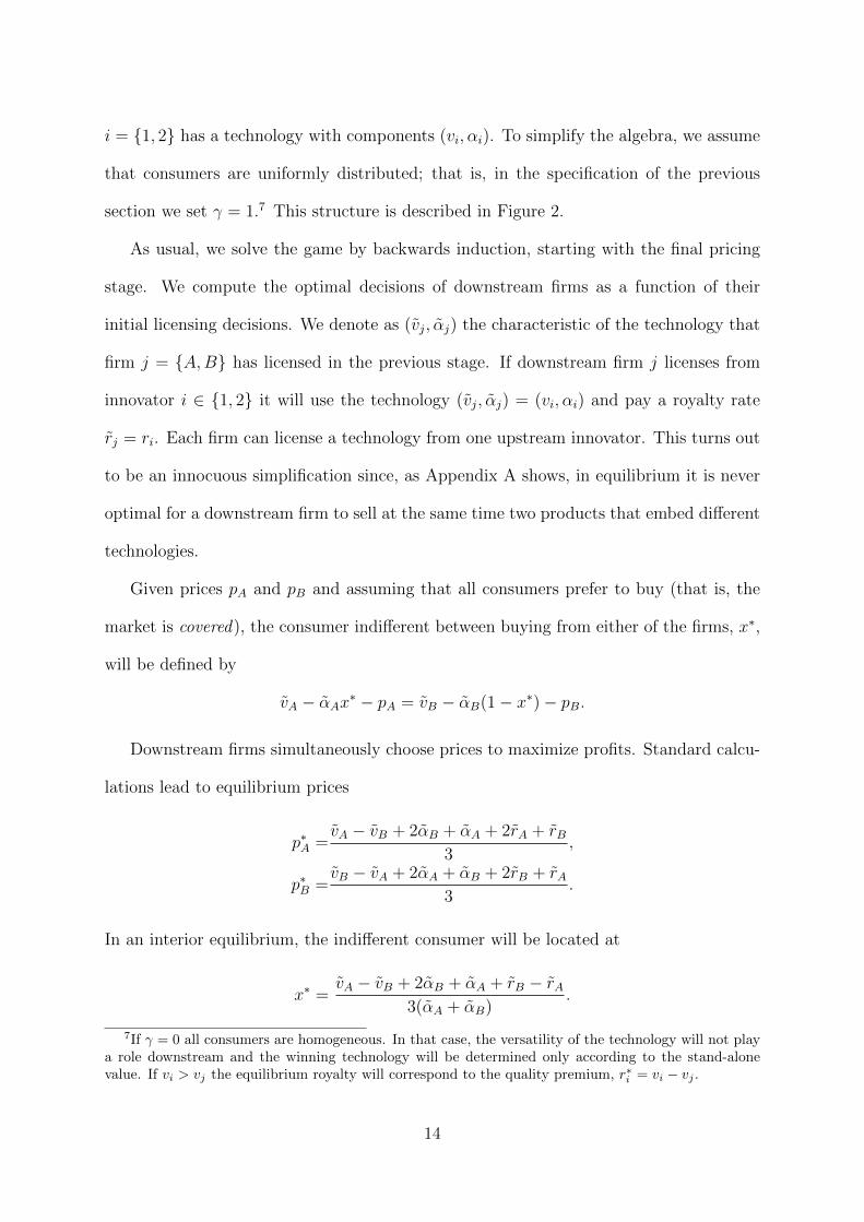
i = {1, 2} has a technology with components (vi, αi). To simplify the algebra, we assume
that consumers are uniformly distributed; that is, in the specification of the previous
section we set γ = 1.7 This structure is described in Figure 2.
As usual, we solve the game by backwards induction, starting with the final pricing
stage. We compute the optimal decisions of downstream firms as a function of their
initial licensing decisions. We denote as (vj, αj) the characteristic of the technology that
firm j = {A,B} has licensed in the previous stage. If downstream firm j licenses from
innovator i ∈ {1, 2} it will use the technology (vj, αj) = (vi, αi) and pay a royalty rate
rj = ri. Each firm can license a technology from one upstream innovator. This turns out
to be an innocuous simplification since, as Appendix A shows, in equilibrium it is never
optimal for a downstream firm to sell at the same time two products that embed different
technologies.
Given prices pA and pB and assuming that all consumers prefer to buy (that is, the
market is covered), the consumer indifferent between buying from either of the firms, x∗,
will be defined by
vA − αAx∗ − pA = vB − αB(1− x∗)− pB.
Downstream firms simultaneously choose prices to maximize profits. Standard calcu-
lations lead to equilibrium prices
p∗A =vA − vB + 2αB + αA + 2rA + rB
3,
p∗B =vB − vA + 2αA + αB + 2rB + rA
3.
In an interior equilibrium, the indifferent consumer will be located at
x∗ =vA − vB + 2αB + αA + rB − rA
3(αA + αB).
7If γ = 0 all consumers are homogeneous. In that case, the versatility of the technology will not playa role downstream and the winning technology will be determined only according to the stand-alonevalue. If vi > vj the equilibrium royalty will correspond to the quality premium, r∗i = vi − vj .
14

I1 I2
A B
0 1x∗
r1r1 r2
r2
pA pB
Figure 2: Structure of the game.
Equilibrium profits are obtained as
Π∗A = (p∗A − rA)x∗ =(vA − vB + 2αB + αA + rB − rA)2
9(αA + αB), (1)
Π∗B = (p∗B − rB)(1− x∗) =(vB − vA + 2αA + αB + rA − rB)2
9(αB + αA). (2)
We can now turn to the first stage, where we will consider the case in which innovators
compete to have their innovation adopted by one or more downstream competitors and the
case of an SSO that decides to standardize a unique technology. We will restrict ourselves
to the case in which an innovator offers the same royalty to the two downstream firms.
Furthermore, in order to reduce the number of cases that may emerge we will assume
that the second firm produces a (completely) versatile technology. That is, we assume
that the technology firm 2 owns generates the same value to all final consumers regardless
of x, which implies that α2 = 0. As a result, when at least one downstream firm adopts
the technology of firm 2 the market will be covered, as postulated above.
An important difference between this case and the one we discussed in the previous
section is that the willingness to pay of a downstream producer now will depend not only
on the technology that it licenses but also on the technology licensed by the competitor
in the final market. In particular, when downstream producers choose their technology
15
independently we need to consider three cases depending on the technology adopted by
the competitor. Specifically, both firms could license the (versatile) technology from
innovator 2, both firms could license a (specific) technology from innovator 1 or, finally,
each firm could license a different technology. In this last case, without loss of generality,
we assume that firm B licenses the (versatile) technology of firm 2.
4.1 The Pricing Equilibrium
If both firms license the technology from innovator 2 they will both produce a good
that consumers regard as homogeneous due to the zero transportation cost (α2 = 0).
Thus, equilibrium prices of the final good converge to marginal cost, p∗A = p∗B = r2, and,
consequently, downstream producers make zero profits, Π∗A = Π∗B = 0. Similarly, if both
downstream producers license the technology of firm 1, their profits, according to (1) and
(2), correspond to
Π∗A = Π∗B =α1
2.
Finally, the third and last case is the equilibrium in which downstream producer A licenses
from innovator 1 and producer B licenses from innovator 2. From (1) and (2) we can
write the profits of downstream firms as
Π∗A =(v1 − v2 + α1 + r2 − r1)2
9α1
,
Π∗B =(v2 − v1 + 2α1 + r1 − r2)2
9α1
.
The previous expression requires firm demands to be well-defined so that
x∗ =v1 − v2 + α1 + r2 − r1
3α1
∈ [0, 1]. (3)
This condition will be satisfied if
v1 − v2 + α1 ≥ r1 − r2 ≥ v1 − v2 − 2α1. (4)
16
4.2 Technology Choice
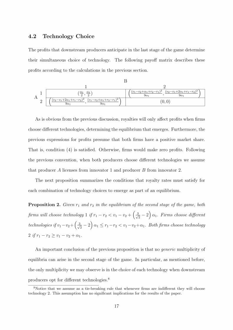
The profits that downstream producers anticipate in the last stage of the game determine
their simultaneous choice of technology. The following payoff matrix describes these
profits according to the calculations in the previous section.
A
B1 2
1 (α1
2, α1
2)
((v1−v2+α1+r2−r1)2
9α1, (v2−v1+2α1+r1−r2)2
9α1
)2
((v2−v1+2α1+r1−r2)2
9α1, (v1−v2+α1+r2−r1)2
9α1
)(0, 0)
As is obvious from the previous discussion, royalties will only affect profits when firms
choose different technologies, determining the equilibrium that emerges. Furthermore, the
previous expressions for profits presume that both firms have a positive market share.
That is, condition (4) is satisfied. Otherwise, firms would make zero profits. Following
the previous convention, when both producers choose different technologies we assume
that producer A licenses from innovator 1 and producer B from innovator 2.
The next proposition summarizes the conditions that royalty rates must satisfy for
each combination of technology choices to emerge as part of an equilibrium.
Proposition 2. Given r1 and r2 in the equilibrium of the second stage of the game, both
firms will choose technology 1 if r1 − r2 < v1 − v2 +(
3√2− 2)α1. Firms choose different
technologies if v1−v2+(
3√2− 2)α1 ≤ r1−r2 < v1−v2+α1. Both firms choose technology
2 if r1 − r2 ≥ v1 − v2 + α1.
An important conclusion of the previous proposition is that no generic multiplicity of
equilibria can arise in the second stage of the game. In particular, as mentioned before,
the only multiplicity we may observe is in the choice of each technology when downstream
producers opt for different technologies.8
8Notice that we assume as a tie-breaking rule that whenever firms are indifferent they will choosetechnology 2. This assumption has no significant implications for the results of the paper.
17
This proposition also sheds some light on the characteristics of the technology that
facilitates the licensing to downstream producers. It is easy to observe that, as opposed
to the case of a downstream monopolist, there might be situations in which technology 2
is preferable for society because it provides a higher dollar value and greater versatility
than technology 1 and yet in equilibrium it is not adopted. In particular, if the value
difference is small, v1 < v2 < v1 + α1, downstream competitors will not be willing to
adopt the technology 2 even if it is offered at the same royalty rate as technology 1.
The reason is that the use of the versatile technology implies fiercer competition with the
other downstream producer, which leads to lower prices for the final product. As a result,
the royalty that innovator 1 can charge is decreasing in the versatility of technology 1
(i.e, decreasing in α1); the more versatile is technology 1 the less sheltered downstream
firms are from competition if they switch to that technology, and the lower must be r1.
The previous proposition allows us to compute the sales of products embedding each
technology. For innovator 1, downstream demand for its technology, denoted as D1(r1, r2)
can be written as
D1(r1, r2) =
0 if r1 > v1 − v2 + α1 + r2,v1−v2+2α1+r2−r1
3α1∈ (0, 1) if v1 − v2 +
(3√2− 2)α1 + r2 ≤ r1 < v1 − v2 + α1 + r2,
1 otherwise.
whereas the demand for innovator 2, D2(r2, r1), can be derived as
D2(r2, r1) =
0 if r2 > v2 − v1 −
(3√2− 2)α1 + r1,
v2−v1+2α1+r1−r23α1
∈ (0, 1) if v2 − v1 −(
3√2− 2)α1 + r1 ≤ r2 < v2 − v1 − α1 + r1,
1 otherwise.
This demand is induced by the number of downstream firms that choose each technol-
ogy and their pricing behavior. Licensing the technology to downstream producers is just
instrumental to reach final consumers. As a result, the induced demand functions turn
out to be discontinuous. In particular, consider a situation in which each downstream
producer licenses the technology from a different innovator. As developer 2 raises r2 its
licensee raises the price, reducing sales and profits. However, at the point in which the
18

royalty is such that the licensee is indifferent between obtaining a license from firm 1 or
2, characterized by
r2 = v2 − v1 −(
3√2− 2
)α1 + r1, (5)
it is still selling a positive quantity that leads to profits α1
2. Thus, a slightly higher royalty
means that the innovator 2 goes from selling a strictly positive amount to 0 and innovator
1 from selling to part of the market, x∗, to the whole market. Hence the discontinuity.9
4.3 Equilibrium Royalties
Upstream innovators choose the royalty that maximizes their expected profits,
ri ∈ arg maxri
riDi(ri, rj) for i = 1, 2 and j 6= i. (6)
Once we replace the expression for the demand we see that the equilibrium in the first
stage when firms share the market can take two forms. Depending on parameter values
there is an interior solution in which firms sell to a share of the market or a situation in
which the discontinuity of the demand plays a role. The next lemma states the necessary
conditions for those two equilibria to exist.
Lemma 1. In an equilibrium in which downstream firm A licenses from innovator 1 and
downstream firm B licenses from innovator 2 the resulting royalties are
r∗1 =v1 − v2 + 4α1
3,
r∗2 =v2 − v1 + 5α1
3,
if −4α1 ≤ v1 − v2 ≤ −(
921/4− 5)α1 and
r∗1 =3(
1− 2−14
)α1,
r∗2 =v2 − v1 + (5− 3× 234 )α1,
9Notice that this discontinuity does not occur when r2 is low in order to license to both downstreamproducers. The reason is that the value of r2 for which both downstream producers want to license fromdeveloper 2 is one in which they make zero profits from using the other technology, which occurs if underthat technology they already obtain 0 sales.
19

if −(
921/4− 5)α1 ≤ v1 − v2 < (5− 3× 2
34 )α1.
This lemma shows that the two technologies can be used in equilibrium in two different
royalty-rate configurations. First, if the stand-alone value of technology 2 is sufficiently
high, compared to technology 1, both upstream producers will choose the royalty that
results from the interior solution to (6). No firm will benefit from undercutting its
competitor. Second, if the difference in stand-alone value v1 − v2 is sufficiently high the
interior solution will not be the equilibrium royalties. At those royalty rates innovator
1 will be interested in undercutting innovator 2 in order to attract downstream firm B
and as a result serve the whole market. This occurs because demand for both firms is
discontinuous. Innovator 2 can prevent innovator 1 from serving the whole market by
lowering the royalty r2. The second part of the previous lemma describes the equilibrium
in which innovator 2 chooses the highest value of r2 which does not trigger a royalty by
innovator 1 that steals all the market. The royalty r1 is obtained as the best response to
that r2, using (6).10
When the stand-alone value of one of the technologies is notably higher than the one
of the competitor that firm grabs the whole market in equilibrium. The royalty rate that
emerges in that case is the result of limit pricing: the highest possible royalty that does
not allow the competitor to lower its royalty and attract at least one of the downstream
producers. The next proposition characterizes the equilibrium in the first stage.
Proposition 3 (Equilibrium Royalties). Assume that α1 ≤ 2v23√2−1 so that the market
is always covered in equilibrium. When downstream producers choose their technology
independently, four possible equilibria may exist depending on the difference v1 − v2.
1. If v1−v2 ≤ −4α1, only upstream producer 2 licenses its technology. The equilibrium
10Innovator 2 will never find it optimal to undercut innovator 1 in order to lure downstream producerA. The reason is that, as pointed out before, this producer anticipates that if both downstream firmsuse the same (homogeneous) technology profits will be 0.
20

royalties correspond to
r∗1 =0,
r∗2 =v2 − v1 − α1.
2. If −4α1 ≤ v1 − v2 ≤ −(
921/4− 5)α1 each innovator sells to only one downstream
firm and sets royalties
r∗1 =v1 − v2 + 4α1
3,
r∗2 =v2 − v1 + 5α1
3.
3. If −(
921/4− 5)α1 ≤ v1 − v2 ≤ (5 − 3 × 2
34 )α1 each innovator sells to only one
downstream firm and sets royalties
r∗1 =3(
1− 2−14
)α1,
r∗2 =v2 − v1 + (5− 3× 234 )α1.
4. If v1 − v2 > (5 − 3 × 234 )α1 only upstream producer 1 licenses its technology. The
equilibrium royalties correspond to
r∗1 =v1 − v2 +
[3√2− 2
]α1,
r∗2 =0.
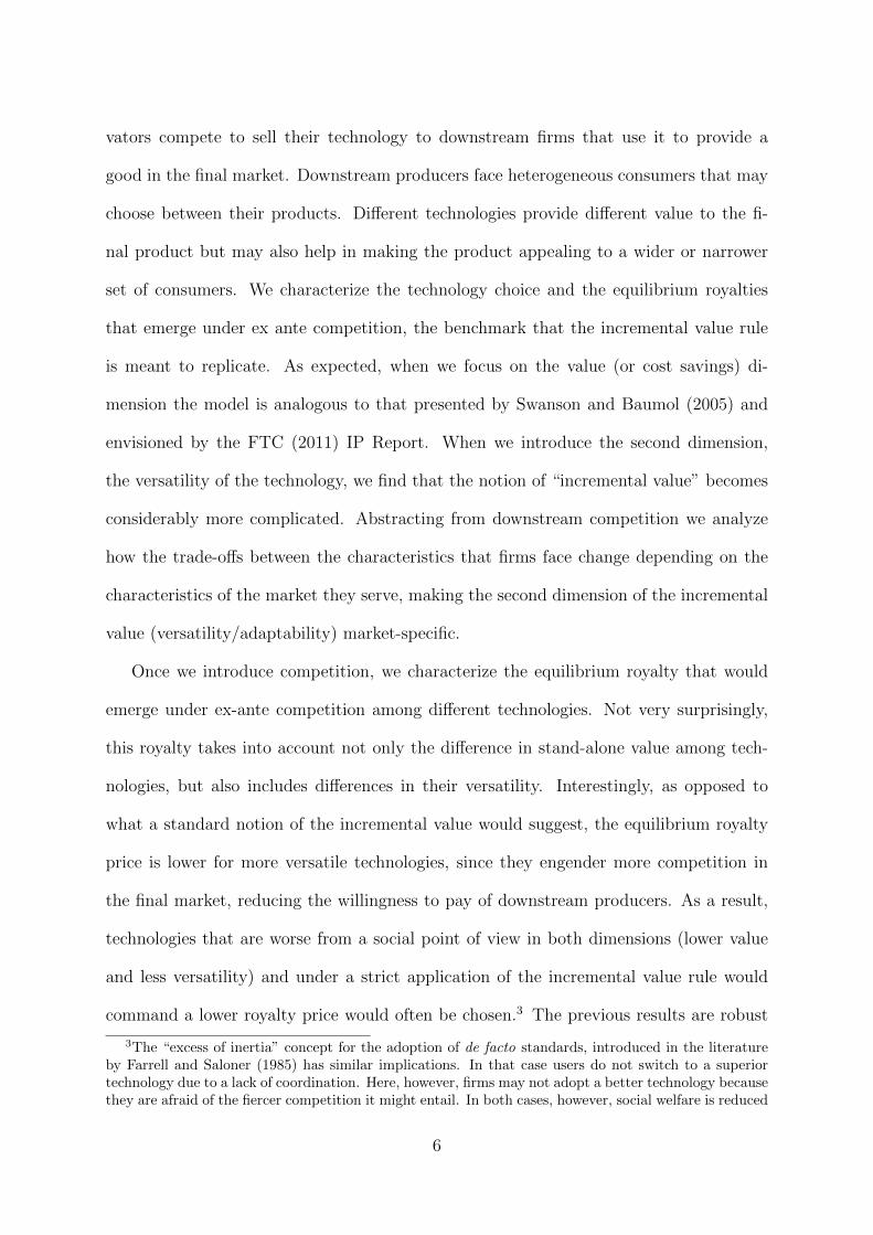
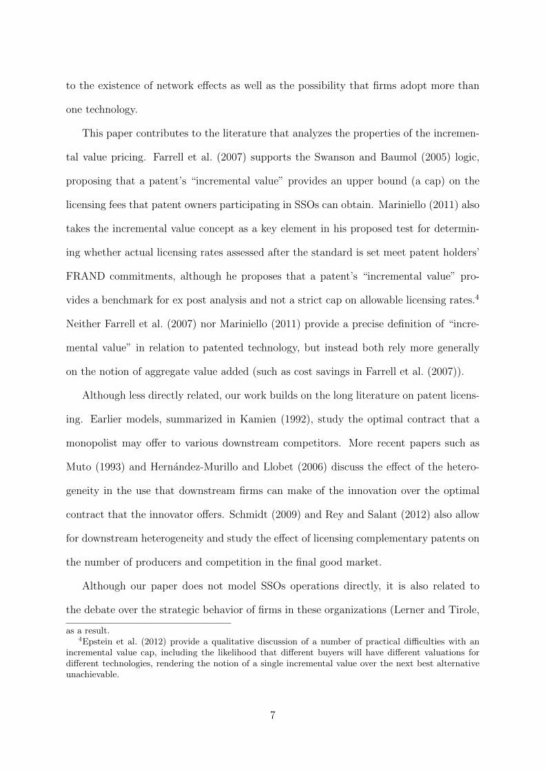
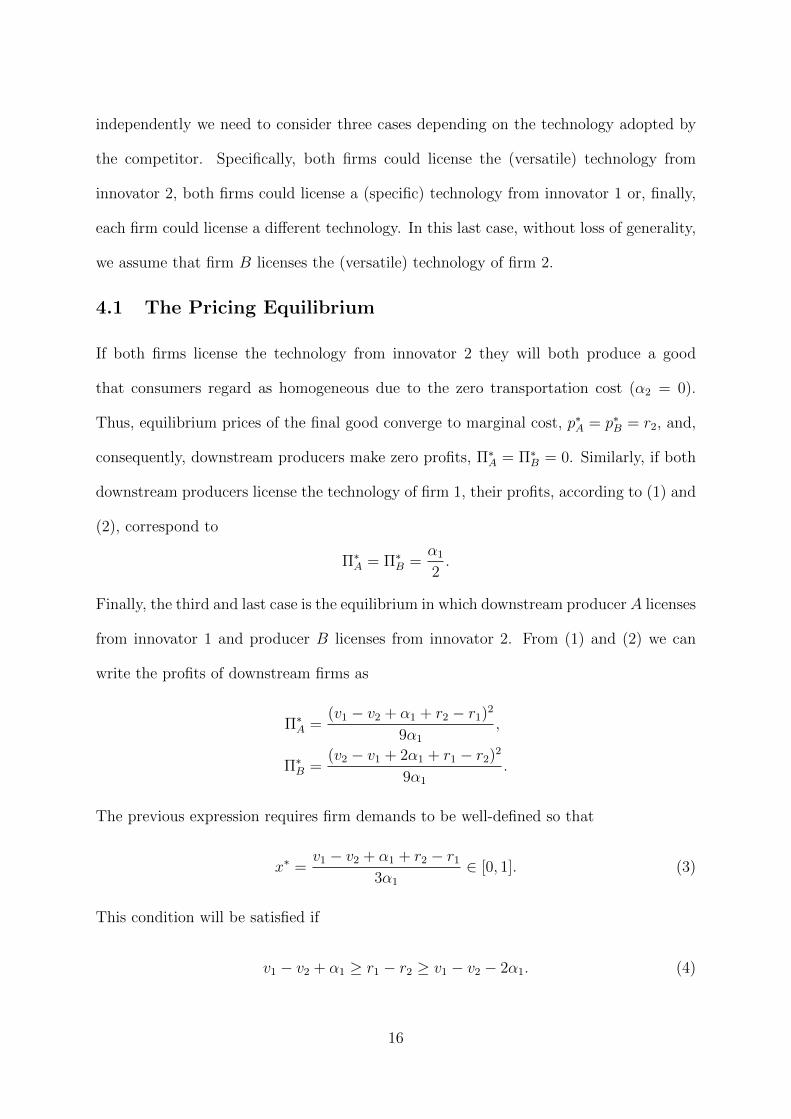
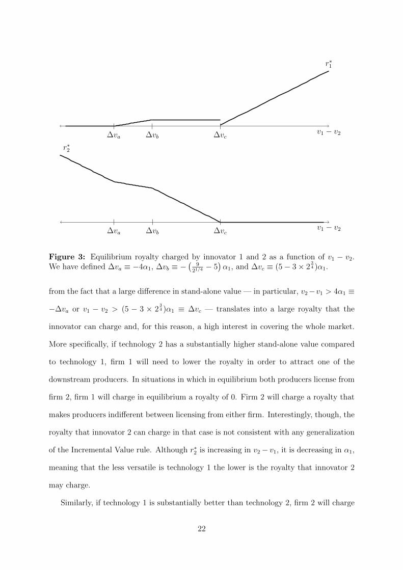
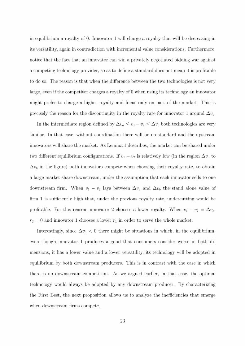
The characteristics of the equilibrium royalty rate in Proposition 3 can be better ex-
plained using Figure 3. This figure represents the equilibrium royalty that both upstream
firms charge as a function of the difference in the stand-alone value of both innovations.
As expected, the royalty that each innovator can charge is, for the most part, increasing
in its stand-alone value advantage with respect to the competitor.
The proposition shows that when one of the technologies has a much higher stand-
alone value that technology will be the only one used in equilibrium. This result arises
21
v1 − v2
r∗1
∆va ∆vb ∆vc
v1 − v2
r∗2
∆va ∆vb ∆vc
Figure 3: Equilibrium royalty charged by innovator 1 and 2 as a function of v1 − v2.We have defined ∆va ≡ −4α1, ∆vb ≡ −
(9
21/4− 5)α1, and ∆vc ≡ (5− 3× 2
34 )α1.
from the fact that a large difference in stand-alone value — in particular, v2−v1 > 4α1 ≡
−∆va or v1 − v2 > (5 − 3 × 234 )α1 ≡ ∆vc — translates into a large royalty that the
innovator can charge and, for this reason, a high interest in covering the whole market.
More specifically, if technology 2 has a substantially higher stand-alone value compared
to technology 1, firm 1 will need to lower the royalty in order to attract one of the
downstream producers. In situations in which in equilibrium both producers license from
firm 2, firm 1 will charge in equilibrium a royalty of 0. Firm 2 will charge a royalty that
makes producers indifferent between licensing from either firm. Interestingly, though, the
royalty that innovator 2 can charge in that case is not consistent with any generalization
of the Incremental Value rule. Although r∗2 is increasing in v2− v1, it is decreasing in α1,
meaning that the less versatile is technology 1 the lower is the royalty that innovator 2
may charge.
Similarly, if technology 1 is substantially better than technology 2, firm 2 will charge
22
in equilibrium a royalty of 0. Innovator 1 will charge a royalty that will be decreasing in
its versatility, again in contradiction with incremental value considerations. Furthermore,
notice that the fact that an innovator can win a privately negotiated bidding war against
a competing technology provider, so as to define a standard does not mean it is profitable
to do so. The reason is that when the difference between the two technologies is not very
large, even if the competitor charges a royalty of 0 when using its technology an innovator
might prefer to charge a higher royalty and focus only on part of the market. This is
precisely the reason for the discontinuity in the royalty rate for innovator 1 around ∆vc.
In the intermediate region defined by ∆va ≤ v1− v2 ≤ ∆vc both technologies are very
similar. In that case, without coordination there will be no standard and the upstream
innovators will share the market. As Lemma 1 describes, the market can be shared under
two different equilibrium configurations. If v1 − v2 is relatively low (in the region ∆va to
∆vb in the figure) both innovators compete when choosing their royalty rate, to obtain
a large market share downstream, under the assumption that each innovator sells to one
downstream firm. When v1 − v2 lays between ∆va and ∆vb the stand alone value of
firm 1 is sufficiently high that, under the previous royalty rate, undercutting would be
profitable. For this reason, innovator 2 chooses a lower royalty. When v1 − v2 = ∆vc,
r2 = 0 and innovator 1 chooses a lower r1 in order to serve the whole market.
Interestingly, since ∆vc < 0 there might be situations in which, in the equilibrium,
even though innovator 1 produces a good that consumers consider worse in both di-
mensions, it has a lower value and a lower versatility, its technology will be adopted in
equilibrium by both downstream producers. This is in contrast with the case in which
there is no downstream competition. As we argued earlier, in that case, the optimal
technology would always be adopted by any downstream producer. By characterizing
the First Best, the next proposition allows us to analyze the inefficiencies that emerge
when downstream firms compete.
23

Proposition 4 (First Best). Assume α1 ≤ 2v23√2−1 . In the First Best the market is covered.
Both producers adopt technology 2 if and only if v2 − v1 ≥ 0. Each producer adopts a
different technology if(
1− 1√2
)α1 < v2 − v1 < 0. Otherwise, both producers choose
technology 1.
Notice that as opposed to the equilibrium solution, technology 2 is always uniquely
adopted when it is superior in both dimensions to technology 1, indicating that down-
stream competition biases the decisions towards technology 1 if that allow firms to set
higher downstream prices. Furthermore, in contrast with the equilibrium outcome, in
the First Best technology 2 is sometimes used by one of the firms even if its stand-alone
value is lower.
Finally, we can compare the previous two technology adoption benchmarks with what
would occur if downstream producers, together, chose which technologies to adopt. This
behavior assumes that firms coordinate only in the technology that will be sponsored
while allowing producers to compete in the sale of the final product.11 In particular, we
assume that an SSO maximizes the profits of its members, in this case the downstream
producers.12 As the next proposition shows, technology 1 is preferred by the both down-
stream producers for a large region of parameters. This region includes not only the case
in which under independent negotiation both firms select different technologies but also
some values for which both firms choose technology 2.
Proposition 5. If v1 ≥ v2−α1 an SSO that maximizes producer profits will always adopt
technology 1 for all its members. The equilibrium royalties would be r∗2 = 0 and
r∗1 =
{v1 − 3
2α1 if v2 ≥ 5
2α1,
v1 − v2 − 114α1 + 3
4
√8α1v2 + 5α2
1 otherwise.
11Notice that since network effects are absent in this section it may not necessarily lead to an agreementaround a unique technology.
12In the model, to the extent that an SSO maximized the profits of all upstream and downstreamproducers it will lead to the first best allocation, since market power in the linear city does not generatea dead-weight loss through higher than optimal prices. Nevertheless, in many informal fora and SSOs,downstream producers (the implementers) comprise a higher proportion of the membership.
24

Notice that the previous result implies a standardization around technology 1 in spite
of the fact that consumer utility does not depend on the technology that defines the
products other consumers purchase. Instead, the reason for the previous result is that
under joint technological negotiation the power of innovator 1 is reinforced, since there is
no threat that potential licensees unilaterally deviate and license technology 2 when v2
is sufficiently high. The SSO might be willing to accept a higher royalty if its members
can pass through the increase in the marginal cost in the form of higher product prices,
without affecting sales much (as is the case in the linear city model for which quantity
stays constant when valuation is high). The alternative of switching to technology 2 is
less appealing due to the fiercer competition it engenders.
5 Network Effects
One of the reasons why SSOs emerge is the need to standardize the technologies underly-
ing the products that firms sell in order to benefit from the network effects that enhance
the valuation consumers place on the product. The model in the previous section did
not include those effects, and for this reason, downstream firms had little incentive to
coordinate their technology adoption decisions. The lack of network effects led to a region
in which both technologies could coexist if they had similar stand-alone values.
In this section we take the opposite extreme view and assume that network effects
are so large that the product is valuable to consumers if and only if all of them purchase
a product that embeds the same technology. In particular, we assume that a consumer
located at a distance x from the downstream firm obtains a utility vi − αi − x − pi
when buying from producer i for i = A,B if all consumers buy a product that uses the
same technology, and 0 otherwise. Notice that this implies that technologies 1 and 2 are
incompatible.
Previous calculations indicate that in the second stage, after royalties have been set,
25

downstream firms anticipate that if both firms choose technology 2 their profits will be
0. The extreme network effects that we assume here also imply that profits will be 0 if
downstream producers choose different technologies.13
To the extent that innovator 1 chooses a royalty that guarantees positive profits to
downstream producers, it will be their (weakly) dominant strategy to adopt technology 1.
In our previous calculations, when both downstream producers chose technology 1 their
profits were equal to Πi = α1
2. These profits, as it is common in the linear city model, were
obtained by assuming that the indifferent consumer obtained a strictly positive utility
from buying. In other words, we assumed that v1 was sufficiently large for the market to
be covered. Under the network effects assumed in this section, technology 1 is relevant to
the extent that even the consumer furthest away from each of the downstream producers
— that is, the consumer located at x = 12
— enjoys positive utility at a price of 0, or
v1 ≥ α1
2. In that case we denote the technology as viable. The next proposition shows
that whenever technology 1 is viable it will be chosen in equilibrium.
Proposition 6. With extreme network effects technology 1 is chosen if and only if it is
viable, v1 ≥ α1
2. In that case equilibrium royalties will be r∗1 = v1 − α1
2and r∗2 ≥ 0.
Some comments about the previous proposition are in order. Developer 1 finds it
optimal to raise the royalty rate r1 up to the point in which the indifferent consumer
in the final market obtains 0 utility. Interestingly, this also implies that downstream
producers choose a price p∗i = r∗1 and obtain 0 profits. The reason is that if they raised
the price, some consumers would obtain negative utility from buying, resulting in the
loss of the network effects and no equilibrium sales. This result is a consequence of the
complementarity that the network effects introduce in the purchasing decision of all final
13Results would be essentially unchanged if we assumed that network effects arose from the technologyadoption of firms. Instead, if network effects only operated by increasing the utility that consumersenjoyed (depending on how many other consumers bought a product with the same technology), profitsfrom choosing different technologies could still be positive and regions in which both technologies coexistin equilibrium might still be possible, just as in the benchmark model.
26

consumers.
It is also important to point out that in equilibrium the royalty that firms will charge
will be independent of the value of the technology that developer 2 brings to the table.
Downstream competition also implies that any positive royalty rate for innovator 2 will be
inconsequential to the equilibrium, since in no circumstances its technology will be chosen.
Furthermore, if downstream developers could cooperatively choose a unique technology,
while still competing in the final market, the result would be unchanged.
Corollary 1. If downstream producers choose the technology cooperatively and compete
in the final market the results are identical as if firms chose technology independently.
In contrast, the First Best will factor in the characteristics of the technologies in both
dimensions and balance them optimally. Thus, technology 1 should only be chosen to the
extent that its stand-alone value is sufficiently higher to compensate its lower versatility
compared to technology 2.
Proposition 7. Under extreme network effects it is socially optimal that both firms adopt
technology 1 as opposed to technology 2 if and only if v1 ≥ v2 + α1
2.
Comparing this case to the one in the previous section we observe that competition
operates in the same way, reducing the range of values under which the versatile tech-
nology 2 will emerge in equilibrium. Under network effects, the bias is stronger, because
adoption of technology 2 by one of the producers implies Bertrand competition, since
the competitor has to adopt the same technology, and this hinders the adoption of this
technology in the first place.
6 Policy Implications for the Incremental Value Rule
The literature on FRAND licensing has focused thus far on appropriate benchmarks for
determining whether or not a particular licensing offer made by the holder of a standard
27
essential patent satisfies the FRAND commitment to an SSO. It is in this context that
the traditional pricing theory of “incremental value” has been proposed. The policy
motivation for the proposal is clear: making FRAND assessments more precise so that
ex post licensing terms and conditions are appropriately tied to the value the patented
technology provides to the standard and do not include any element of holdup derived
from market power gained through the standard setting process. But in the quest for more
transparent rules for FRAND licensing, we must keep in mind the real world complexities
that such rules must operate within. The model we develop above addresses one such
complexity: the common incidence that technologies considered for inclusion in a standard
must be evaluated on multiple dimensions, at least some of which cannot be easily reduced
to an ordinal measure. We find that multi-dimension technologies involving either-or
trade-offs introduce a number of difficulties for implementing an incremental value rule
for FRAND licensing.
Multiple dimensions are not problematic in themselves, as a large literature demon-
strates how scoring functions can be employed to express those dimensions within a single,
easily compared index (Asker and Cantillon, 2008). And in the simplest version of our
model, presented in section 3 we show that a scoring function could work to aggregate
multiple dimensions of a technology when the firms licensing that technology do not face
any downstream competition. Specifically, in section 3 we find that while a downstream
monopoly restricts the quantity sold in the final market it does not alter the choice of
technologies upstream, which depend on a score of the different dimensions. This score
can be understood as a generalization of the incremental value rule, which would account
not only for the traditional value enhancement or “cost savings” aspect typically used in
discussions of applying the rule to patent licensing, but also for more complex aspects
of the technology that affect the characteristics of the final products, such as the ability
of downstream implementers to adapt the technology so as to target their products to
28
narrow market niches. Even here, however, the scoring function is not straightforward,
though, as the scoring function contains an endogenous variable, γ.14
Downstream competition, however, changes things radically. Whereas more versatile
(non-specific) technologies tend to benefit a larger proportion of consumers, the fiercer
competition that such technologies induce for licensees reduces the technologies’ appeal
to firms that sell in the final market. The example in which no network effects are
present in the market, developed in section 4, illustrates the strategic side of technology
choices made in cooperative standard setting. The mismatch in incentives surrounding
technology choice is apparent from a comparison of Proposition 3 which defines the profit
maximizing choices downstream firms will make depending on the relative comparison of
the value enhancement aspect of the two technologies and Proposition 4, which defines
the First Best technology choice from a social perspective. This last proposition shows
that to achieve the social optimum, the versatile technology 2 should be used whenever
it is (at least) as good in terms of the stand-alone value dimension as the differentiated
technology 1. In the equilibrium solution, however, it is clear that firms are reluctant to
adopt technology 2 unless it yields an increase in value sufficiently large to “overcome”
the competitive disadvantage motivated by its higher versatility.
The presence of network effects, considered in section 5, makes implementing firms’
strategic choices even more apparent. In the limit case we consider, the versatile technol-
ogy 2 is never used as long as the differentiable technology 1 is viable. As some degree of
network effects are a likely explanation for emergence of cooperative interoperability stan-
dards, the results in section 4 likely understate the extent to which strategic competitive
concerns affect technology choices within SSOs.
These results suggest that in the presence of competition, imposing any sort of rule
14The other difficulty that emerges is how, exactly, to measure the “cost savings” or “price enhancing”aspect of a given technology, regardless of the presence of any other dimensions that must be comparedas well in order to determine an “increment”.
29
based on some sort of score of the value dimension of a given technology is unlikely
to reach an efficient outcome. In fact, the imposition of an incremental value rule for
FRAND licensing is likely to tilt technology adoption towards those that soften down-
stream competition. In our benchmark example, a rule that rewarded technology 2 for
its higher versatility would lead to a lower adoption of that technology as compared to
ex ante equilibrium technology choices: the equilibrium in which both firms adopt the
versatile technology 2 – when v1 − v2 ≤ −4α1 in Proposition 3 – provides a royalty r∗2
that is lower than v2 − v1 and that is actually increasing, rather than decreasing, in the
versatility of the other technology.
Under the circumstances we study in this paper, there is little room for a competi-
tion agency to improve on outcomes. Consider first the case of downstream monopolies.
Absent the concern about intensified competition in the downstream market that comes
from the more versatile technology, downstream monopolists freely choose to license the
more versatile technology as long as the difference in the stand-alone value dimension for
the narrower technology is not too large; this outcome matches the First Best (see Propo-
sition 1). Hence there is nothing for an agency to improve upon in this case. However,
when downstream markets are competitive (which is often the goal and the realization
for cooperative standard setting), agencies would be faced with the task of recreating
not only the rank ordering of the technologies considered during the development of a
standard in terms of any measurable value enhancements or “cost savings” (the v di-
mensions), but also in terms of any strategic dimensions of the competing technologies
(the α dimensions). SSO meeting minutes and other documentation may contain con-
temporaneous comparisons of competing technological solutions on observable measures
(e.g., transmission speed or bit error rates), but those records are unlikely to contain any
information on the strategic elements of product differentiation.
Moreover, even for technologies that compete solely on definable characteristics, those
30
characteristics may often involve trade-offs that pit one member’s preference set against
another’s. For example, reliability versus cost is a common trade-off across many technol-
ogy fields – technology A may involve “cost savings” as compared to technology B, but
B is viewed as considerably more “reliable” than A. Looking solely at the “cost savings”
dimension would be misleading for any “incremental value” calculation. But since “cost
savings” move inversely with “reliability” under this trade-off, combining both dimensions
in a scoring function is unlikely to be helpful either: such an index would simply suggest
the midpoint compromise, with moderate cost and moderate reliability, whereas product
markets may be more likely to dictate a solution closer to one or the other extreme.
Firms implementing the same standard but in different end products are likely to view
trade-offs of this sort quite differently. An SSO vote is likely to accurately reflect the ma-
jority view of these trade-offs, but recreating that complex comparison ex post, say with
a constructed scoring function, is likely to be difficult at best. Such information should
of course be collected when feasible, as it could nonetheless inform FRAND assessments,
but the hope for a formulaic incremental value calculation strikes us as unrealistic.
When private concerns, such as end product differentiation and market competition,
are included in the calculus as well, we could even find that one firm’s “benefit” is
another firm’s “detriment.” In this case, an ex post scoring function would be entirely
unworkable. Nor are we likely to uncover information of this sort in any forensic dig
through SSO documents, though individual firm records may be informative nonetheless.
We might think that private benefits should be excluded, in the interest of social good,
from any “incremental value” calculation for a FRAND assessment, but if the task is
to determine what licensing fees are reasonable for a particular implementer to pay for
access to a FRAND-encumbered patent, then private value is very much relevant.15
15Private value is embedded in the Georgia-Pacific factors that guide reasonable royalty assessmentsin patent infringement cases in US courts.
31
References
Asker, J., and Cantillon, E., 2008, “Properties of scoring auctions,” RAND Journal
of Economics, 39: 69–85.
Brooks, R. G., and Geradin, D., 2011, “Taking Contracts Seriously: The Meaning
of the Voluntary Commitment to License Essential Patents on ”Fair and Reasonable”
Terms,” in S. Anderman and A. Ezrachi, eds., Intellectual Property and Compe-
tition Law New Frontiers.
Epstein, R., Kieff, F. S., and Spulber, D. F., 2012, “The FTC, IP, and SSOs:
Government Hold-Up Replacing Private Coordination,” Journal of Competition Law
and Economics, 8: 1–46.
Farrell, J., Hayes, J., Shapiro, C., and Sullivan, T., 2007, “Standard Setting,
Patents and Hold-up,” Antitrust Law Journal, 74: 603–670.
Farrell, J., and Katz, M. L., 2005, “Competition Or Predation? Consumer Coordi-
nation, Strategic Pricing And Price Floors In Network Markets,” Journal of Industrial
Economics, 53: 203–231.
Farrell, J., and Saloner, G., 1985, “Standardization, Compatibility, and Innova-
tion,” RAND Journal of Economics, 16: 70–83.
FTC, 2011, “The Evolving IP Market Place: Aligning Patent Notice and Remedies with
Competition,” Technical report, U.S. Federal Trade Commission.
Ganglmair, B., Froeb, L. M., and Werden, G. J., 2011, “Patent Hold-Up and An-
titrust: How a Well-Intentioned Rule Could Retard Innovation,” Journal of Industrial
Economics, forthcoming.
Hernandez-Murillo, R., and Llobet, G., 2006, “Patent licensing revisited: Het-
erogeneous firms and product differentiation,” International Journal of Industrial Or-
ganization, 24: 149–175.
Kamien, M. I., 1992, “Patent Licensing,” in R. Aumann and S. Hart, eds., Handbook
of Game Theory, volume 1, chapter 11, Elsevier, 1 edition.
32
Layne-Farrar, A., Llobet, G., and Padilla, J. A., 2013, “Payments and Par-
ticipation: The Incentives to Join Cooperative Standard Setting Efforts,” Journal of
Economics and Management Strategy.
Lerner, J., and Tirole, J., 2006, “A Model of Forum Shopping,” American Economic
Review, 96: 1091–1113.
Mariniello, M., 2011, “Fair, Reasonable and Non-Discriminatory (FRAND) terms: a
challenge for Competition Authorities,” Competition Law and Economics, forthcom-
ming.
Muto, S., 1993, “On Lincensing Policies in bertrand Competition,” Games and Eco-
nomic Behavior.
Negus, K. J., and Petrick, A., 2009, “History of Wireless Local Area Networks
(WLANs) in the Unlicensed Bands,” Info, 11: 36–56.
Rey, P., and Salant, D., 2012, “Abuse of Dominance and Licensing of Intellectual
Property,” IDEI Working Papers 712, Institut d’conomie Industrielle (IDEI), Toulouse,
URL http://ideas.repec.org/p/ide/wpaper/25793.html.
Schmidt, K., 2009, “Complementary Patents and Market Structure,” Discussion Papers
274, SFB/TR 15 Governance and the Efficiency of Economic Systems, Free University
of Berlin, Humboldt University of Berlin, University of Bonn, University of Mannheim,
University of Munich, URL http://ideas.repec.org/p/trf/wpaper/274.html.
Swanson, D. G., and Baumol, W. J., 2005, “Reasonable and Nondiscriminatory
(RAND) Royalties, Standards Selection, and Control of Market Power,” Antitrust Law
Journal, 73.
33

Appendix
A The Licensing of Multiple Technologies
Consider an extension of our basic model in which final good producers can license the
technology from both upstream developers if they choose to do so and sell one product
with each of them. Assume that the timing of the model remains unchanged: Initially
developers set their royalty rates. Downstream producers first simultaneously choose
which products to sell and later they simultaneously set their prices.
Suppose that in the final period a firm, say firm A, has licensed the innovations both
of firm 1 and 2. It is easy to see that in order for the products that embed each of the
innovations to be sold at the same time consumers located close to producer A (at a low
value of x) should buy the product that embeds innovation 1 and consumers further away
from the location of firm A should buy the other product. That is, if we denote as piA
the price of the product that embeds innovation i = 1, 2, then the indifferent consumer
will be characterized by
v1 − α1xA − p1A = v2 − p2A, (7)
so that consumers at x < xA prefer the product that embeds innovation 1.
We now solve for the different combinations of products that can emerge in the final
stage. Our first result shows that in equilibrium it will never be the case that at least one
downstream firm sells the two products and both firms offer the product that embeds the
innovation developed by upstream firm 2.
Lemma 2. When downstream producers can sell more than one product, if in equilibrium
one firm sells both products, the competitor will sell only product 1.
Thus, the previous result suggests that the only case in which firms might sell multiple
products in equilibrium corresponds to the situation in which one of the firms sells two
products, say firm A, and the other (firm B) sells only the product that embeds the
technology of firm 1. If the three products are sold in equilibrium, following the previous
arguments, we will have that consumers between 0 and xA (as defined in equation (7))
buy product 1 from firm A. Consumers between xA and xB buy product 2 from firm A
and consumers between xB and 1 buy from firm B, where xB is defined as
v1 − α1(1− xB)− p1B = v2 − p2A. (8)
34
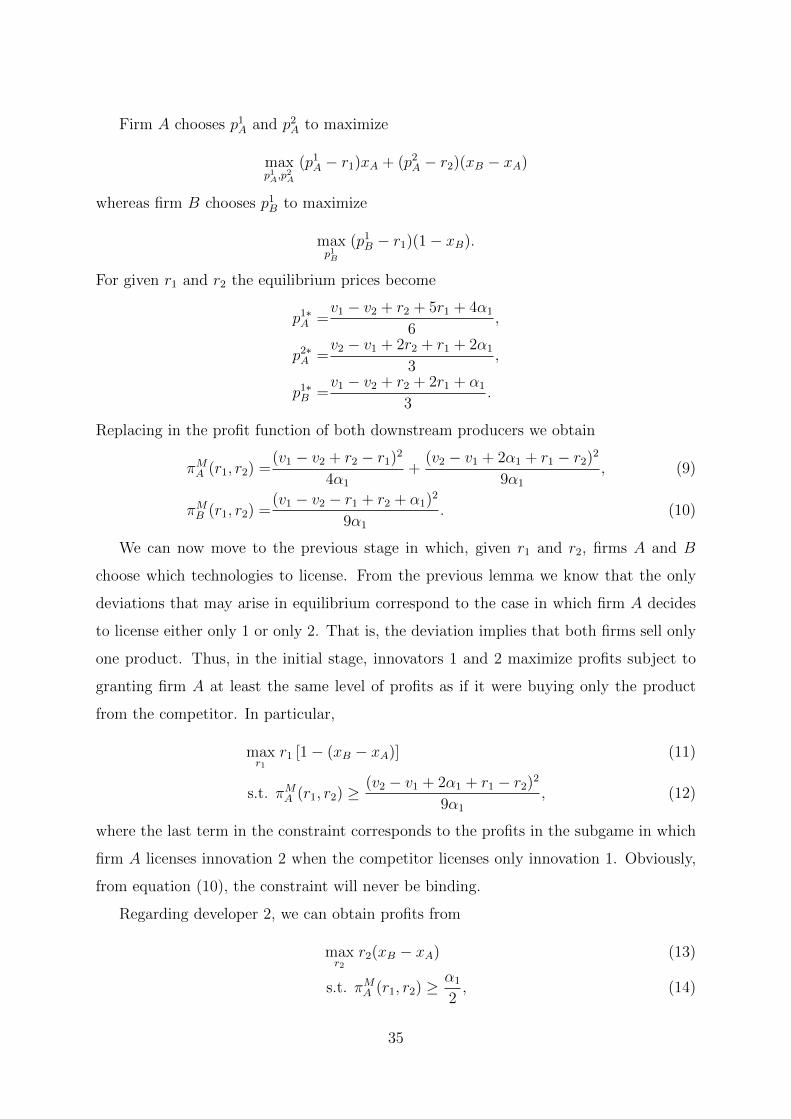
Firm A chooses p1A and p2A to maximize
maxp1A,p
2A
(p1A − r1)xA + (p2A − r2)(xB − xA)
whereas firm B chooses p1B to maximize
maxp1B
(p1B − r1)(1− xB).
For given r1 and r2 the equilibrium prices become
p1∗A =v1 − v2 + r2 + 5r1 + 4α1
6,
p2∗A =v2 − v1 + 2r2 + r1 + 2α1
3,
p1∗B =v1 − v2 + r2 + 2r1 + α1
3.
Replacing in the profit function of both downstream producers we obtain
πMA (r1, r2) =(v1 − v2 + r2 − r1)2
4α1
+(v2 − v1 + 2α1 + r1 − r2)2
9α1
, (9)
πMB (r1, r2) =(v1 − v2 − r1 + r2 + α1)
2
9α1
. (10)
We can now move to the previous stage in which, given r1 and r2, firms A and B
choose which technologies to license. From the previous lemma we know that the only
deviations that may arise in equilibrium correspond to the case in which firm A decides
to license either only 1 or only 2. That is, the deviation implies that both firms sell only
one product. Thus, in the initial stage, innovators 1 and 2 maximize profits subject to
granting firm A at least the same level of profits as if it were buying only the product
from the competitor. In particular,
maxr1
r1 [1− (xB − xA)] (11)
s.t. πMA (r1, r2) ≥(v2 − v1 + 2α1 + r1 − r2)2
9α1
, (12)
where the last term in the constraint corresponds to the profits in the subgame in which
firm A licenses innovation 2 when the competitor licenses only innovation 1. Obviously,
from equation (10), the constraint will never be binding.
Regarding developer 2, we can obtain profits from
maxr2
r2(xB − xA) (13)
s.t. πMA (r1, r2) ≥α1
2, (14)
35

where the last term in the constraint corresponds to the profits in the subgame in which
firm A decides to license only innovation 1.
The next proposition shows that there is no combination of the royalties that satisfies
the previous condition while, at the same time, it guarantees a positive market share for
all products.
Lemma 3. There is no equilibrium in which one firm licenses both technologies and the
competitor licenses only technology 1 and all products have a positive market share.
An immediate consequence, that we summarize in the following proposition, is that
even when firms can create products that embed innovations from both firms they will
choose not to do it.
Proposition 8. In equilibrium each downstream firm will sell a unique product even if
there are no costs of adopting more than one.
The reason is that by adopting a second product (typically from innovator 2) they
make competition fiercer not only with the other firm but also with the other product
that they might be selling. Of course, this result could change if by selling an additional
product, downstream firms not only stole sales from other products in the market but
they also attracted new consumers to the market.
B Proofs
In this section we include the proof of the results of this paper.
Proof of Proposition 1: The downstream producer will prefer the technology of
innovator i over innovator j if πMA (i) ≥ πMA (j). This condition is satisfied if
vi
αγ
1+γ
i
− ri
αγ
1+γ
i
≥ vi
αγ
1+γ
j
− rj
αγ
1+γ
j
.
Bertrand competition among technology producers implies that in equilibrium one of the
firms, say firm j, will set a royalty equal to 0. In that case firm i will optimally set a
positive royalty if and only ifvi
αγ
1+γ
i
≥ vj
αγ
1+γ
j
.
36

Using the previous expressions and replacing r∗j = 0 we obtain the maximum royalty that
firm i can charge and, therefore, the optimal one as
r∗i = vi −(αiαj
) γ1+γ
vj.
In the First Best, social welfare arising from the choice of technology i can be computed
as
W =
∫ viai
0
(vi − αix)γxγ−1dx =vγ+1i
αγi
1
1 + γ,
and the result is immediate.
Proof of Proposition 2: For an equilibrium in which both downstream firms license
technology 1 it has to be that the deviation, choose technology 2, leads to lower profits.
Comparing profits in the different alternatives, it is immediate that lower profits arise
when r1− r2 < v1− v2 +(
3√2− 2)α1. Similarly, for an equilibrium in which both down-
stream producers choose technology 2 it has to be the case that by choosing technology
1 they obtain no demand. This condition implies that r1 − r2 ≥ v1 − v2 + α1. These
two conditions are mutually exclusive meaning that the two equilibria cannot coexist. If
neither condition is satisfied the equilibrium in which firms choose different technologies
arises.
Proof of Lemma 1: The first order condition that determines the solution to the
problem of both upstream producers in the text (equation (6)) leads to reaction functions
rR1 (r2) =v1 − v2 + r2 + α1
2,
rR2 (r1) =v2 − v1 + r1 + 2α1
2.
The intersection of both reaction functions determines the interior solution for the equi-
librium royalty r∗1 = v1−v2+4α1
3and r∗2 = v2−v1+5α1
3. Notice, however, that this result
requires that 4α1 ≥ v2 − v1 ≥ −5α1. These are the same conditions that guarantee that
the indifferent consumer, x∗, lies between 0 and 1.
We now analyze the incentives for an innovator to undercut the competitor. In par-
ticular, consider a given r2. Profits for innovator 1 when the market is shared correspond
to
Π∗1(r2) = maxr1
r1x∗ =
(v1 − v2 + α1 + r2)2
12α1
,
37
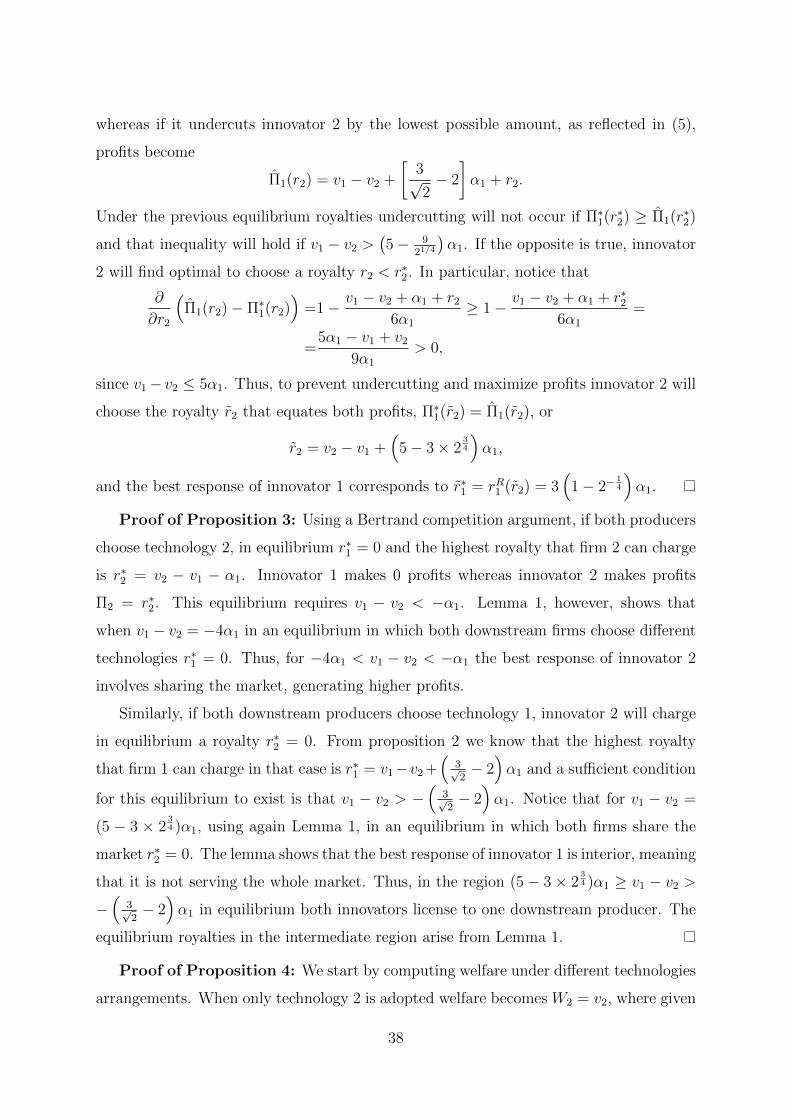
whereas if it undercuts innovator 2 by the lowest possible amount, as reflected in (5),
profits become
Π1(r2) = v1 − v2 +
[3√2− 2
]α1 + r2.
Under the previous equilibrium royalties undercutting will not occur if Π∗1(r∗2) ≥ Π1(r
∗2)
and that inequality will hold if v1 − v2 >(5− 9
21/4
)α1. If the opposite is true, innovator
2 will find optimal to choose a royalty r2 < r∗2. In particular, notice that
∂
∂r2
(Π1(r2)− Π∗1(r2)
)=1− v1 − v2 + α1 + r2
6α1
≥ 1− v1 − v2 + α1 + r∗26α1
=
=5α1 − v1 + v2
9α1
> 0,
since v1− v2 ≤ 5α1. Thus, to prevent undercutting and maximize profits innovator 2 will
choose the royalty r2 that equates both profits, Π∗1(r2) = Π1(r2), or
r2 = v2 − v1 +(
5− 3× 234
)α1,
and the best response of innovator 1 corresponds to r∗1 = rR1 (r2) = 3(
1− 2−14
)α1.
Proof of Proposition 3: Using a Bertrand competition argument, if both producers
choose technology 2, in equilibrium r∗1 = 0 and the highest royalty that firm 2 can charge
is r∗2 = v2 − v1 − α1. Innovator 1 makes 0 profits whereas innovator 2 makes profits
Π2 = r∗2. This equilibrium requires v1 − v2 < −α1. Lemma 1, however, shows that
when v1 − v2 = −4α1 in an equilibrium in which both downstream firms choose different
technologies r∗1 = 0. Thus, for −4α1 < v1 − v2 < −α1 the best response of innovator 2
involves sharing the market, generating higher profits.
Similarly, if both downstream producers choose technology 1, innovator 2 will charge
in equilibrium a royalty r∗2 = 0. From proposition 2 we know that the highest royalty
that firm 1 can charge in that case is r∗1 = v1−v2 +(
3√2− 2)α1 and a sufficient condition
for this equilibrium to exist is that v1 − v2 > −(
3√2− 2)α1. Notice that for v1 − v2 =
(5 − 3 × 234 )α1, using again Lemma 1, in an equilibrium in which both firms share the
market r∗2 = 0. The lemma shows that the best response of innovator 1 is interior, meaning
that it is not serving the whole market. Thus, in the region (5− 3× 234 )α1 ≥ v1 − v2 >
−(
3√2− 2)α1 in equilibrium both innovators license to one downstream producer. The
equilibrium royalties in the intermediate region arise from Lemma 1.
Proof of Proposition 4: We start by computing welfare under different technologies
arrangements. When only technology 2 is adopted welfare becomes W2 = v2, where given
38

the assumption of α2 = 0 the result does not change regardless of whether one firm or
both adopt it.
When both firms adopt different technologies – for example, firm A adopts technology
1 and firm B technology 2 – the market is always covered. Product A is assigned to those
consumers located at x such that v1−α1x > v2. Welfare in this case can be computed as
W12 =
∫ v1−v2α1
0
(v1 − α1x)dx+ v2
(1− v1 − v2
α1
)= v2 +
(v1 − v2)2
2α1
,
with v1 > v2 > v1 − α1.
Finally, if both downstream firms adopt technology 1 the market will be covered if
and only if v1 >α1
2. As a result, social welfare can be computed as
W1 =
{v21α1
if v1 ≤ α1
2,
v1 − α1
4otherwise.
Obviously, if v2 ≥ v1 the unique adoption of technology 2 is optimal. It is immediate that
W2 ≥ W12 and that W2 > W1 if v1 >α1
2. When v1 <
α1
2, notice that since α1 ≤ 2
3√2−1v2
we have that
W2 = v2 ≥3√
2− 1
2α1 >
α1
4≥ W1.
If v2 < v1 we have that W12 > W2. Furthermore, v1 > v2 ≥ 3√2−12
α1 implies that
W1 = v1 − α1
4. It is immediate that W12 > W1 if and only if v2 > v1 −
(1− 1√
2
)α1.
Proof of Proposition 5: First notice that, from the point of view of both down-
stream producers, choosing technology 2 by firms will never be optimal since it would
lead to aggregate profits of 0. If both firms chose different technologies their joint profits
would be
Π1A + Π2
B =(v1 + 2α1 + r2 − r1)2
9α1
+(v2 − v1 + α1 + r1 − r2)2
9α1
,
where v1− v2−2α−1 ≤ r1− r2 ≤ v1− v2 +α1 for both firms to have positive sales under
this technology configuration. It is easy to see that the previous function is a parabola,
with a minimum at v1 − v2 − α1
2. Both extremes constitute the maximum and are equal
and imply profits of α1.
If both firms choose technology 1 and v1 is sufficiently high so that the indifferent
consumer always obtains positive utility, the equilibrium price will be pi = α1 + r∗i for
i = A,B. The indifferent consumer, located at 1/2, will obtain utility
U
(1
2
)= v1 −
α1
2− (α1 + r∗1).
39
If r∗1 ≤ v1 − 32α1 both downstream firms make profits of Π1
i = α1
2so that total profits are
α1, dominating the case in which firms choose different technologies. For royalty rates
r1 ∈(v1 − 3
2α1, v1 + α1
)joint profits of downstream firms correspond to v1 − α1
2− r1
which decrease at a rate of 1 with r1 and the market is still covered in equilibrium.
We now show that in equilibrium both firms license technology 1 as long as v1 −
v2 + α1 > 0. First suppose that v2 ≥ 52α1 so that v1 − 3
2α1 ≥ v1 − v2 + α1. In that
case, r∗1 = v1 − v2 + α1 and r∗2 = 0. A higher r1 will lead to an equilibrium with two
technologies where the market share of the licensee of technology 1 would be 0.
If v2 <52α1 so that v1 − 3
2α1 < v1 − v2 + α1, innovator 1 can raise r1 and still induce
higher profits for the licensee than what they could obtain by relying on two technologies.
Equating both expressions for profits we obtain that such a move is profitable as long as
r1 ≤ v1 − v2 −11
4α1 +
3
4
√8α1v2 + 5α2
1,
which leads to the equilibrium stated in the text.
Proof of Proposition 6: If both downstream producers choose technology 1 and
face a royalty r1 their profits will be defined, for i = A,B, as
Πi = maxpi
(pi − r1)v1 − piα1
,
if all consumers buy,v1 − pAα1
+v1 − pBα1
= 1
and 0 otherwise. If the constraint is not binding, we obtain that in equilibrium p∗A =
p∗B = p∗ = r1 +α1. If v1− α1
2−p∗ < 0 firms must lower their price in order to guarantee a
positive utility to the consumer located at 12. The highest possible royalty that developer
1 could charge while the market remains covered is r∗1 = v1 − α1
2. In this case, each
producer is indifferent between setting pi = r∗1 and covering the market or deviating to
another price.
As mentioned in the text, to the extent that downstream developers obtain positive
profits by choosing technology 1 it is a weakly dominant strategy for both downstream
producers to choose that technology.
Proof of Proposition 7: The expression for social welfare when both producers
adopt technology 1, W1, and both producers adopt technology 2, W2, are derived in
40

Proposition 4 as
W2 =v2
W1 =v1 −α1
4.
where, given the network effects, in the case of technology 1 it is always optimal that the
market is covered. The direct comparison of these expressions leads to the result in the
proposition.
Proof of Lemma 2: In order to prove the previous result we will show that an
allocation in which each firm sells both products or one in which one firm sells both
products and the other sells only product 2 will not arise in equilibrium.
Regarding the latter, suppose first that one firm, say firm A sells both products and
firm B sells only the product that embeds the technology from firm 2. From equation
(7), firm B will only sell if the price for its product p2B is lower or equal than p2A. Since
firm B only sells product 2 it is a dominant strategy to undercut firm A as long as
p2A > r2. Thus, in equilibrium firm A will either sell only the product that embeds the
technology of firm 1 or will choose p2A = p2B = r2. Notice that the first case is equivalent
to firm A not offering product 2 at all. Thus, for the candidate equilibrium to exist it
has to be that p2A = r2. In the previous stage, when firms choose which products to
sell, firm A compares offering both products with, among other options, offering only
product 1. Clearly, the second option is preferred since otherwise first firm A meets more
competition for product 1, while not benefiting from the sale of product 2. Thus, this
candidate equilibrium cannot arise.
Suppose now that both firms license the technology from both upstream producers in
order for each firm to sell both products. According to equation (7), it has to be the case
that consumers located at x ≤ xA buy product 1 from downstream producer A. We can
define xB in a symmetric way. As a result, we conclude that consumers at x ≥ xB ≥ xA
buy product 1 from producer B. Consumers at x ∈ (xA, xB) buy product 2. Thus, at
any price greater than r2 one of the firms will have incentives to undercut the competitor
for the product embedding innovation 2, since it will sell to all consumers between xA
and xB and have a negligible impact on the indifferent consumers themselves. Thus, the
standard Bertrand competition argument will lead to p2A = p2B = r2.
From the previous argument, the indifferent consumer between buying product 1 from
41

firm A and buying product 2, x∗A, corresponds to
v1 − α1x∗A − p1A = v2 − r.
Thus, the price for product 1 that maximizes profits for firm A can be obtained from
maxp1A
(p1A − r1)v1 − v2 − p1A + r2
α1
,
or p1∗A = v1−v2+r2+r12
and lead to profits of π12A = (v1−v2+r2−r1)2
4α1. Notice that for this
equilibrium to exist x∗A = x∗B ≤ 12
implying that v1 − v2 + r2 − r1 ≤ α1.
Moving to the previous stage, suppose now that A has adopted both innovations and
B is considering whether to adopt only innovation 1 or adopting 1 and 2. If firm B adopts
only 1, profits are identical to those of equation (10). The comparison with the profits
when both firms sell both products show that the selling of both products leads to higher
profits if
v1 − v2 + r2 − r1 ≥ 2α1,
which is a contradiction with x∗A = x∗B ≤ 12.
Proof of Lemma 3: The constraint in the problem of developer 2, equation (14),
implies that either
r2 − r1 ≤ v2 − v1 +8− 3
√10
13α1
or
r2 − r1 ≥ v2 − v1 +8 + 3
√10
13α1.
For the solution to lead to positive market share it has to be that 0 < xA < xB < 1. In
particular
xA =v1 − v2 + r2 − r1
2α1
> 0 =⇒ r2 − r1 > v2 − v1,
xB =v2 − v1 − r2 + r1 + 2α1
3α1
< 1 =⇒ r2 − r1 > v2 − v1 − α1,
xA > xB =⇒ r2 − r1 < v2 − v1 +4
5α1.
Since the second condition is implied by the first, we have that for all products to have
a positive market share it has to be that v2 − v1 < r2 − r1 < v2 − v1 + 45α1, and this is
incompatible with the two conditions above, since 8−3√10
13< 0 and 8+3
√10
13> 4
5.
Proof of Proposition 8: Immediate from Lemma 2 and 3.
42