motivation: why inverse problems? - compute.dtu.dkpcha/airtoolsii/tutorial/dublinday1.pdf · 0 20...

DIAS 006 – Discrete Inverse Problems – Day 1 1

Motivation: Why Inverse Problems?

Example: from measurements of the magnetic field on the surface,

we determine the activity magnetization the volcano.

⇒Measurements Reconstruction

on the surface inside the volcano


Another Example: the Hubble Space Telescope

For several years, the HST produced blurred images.


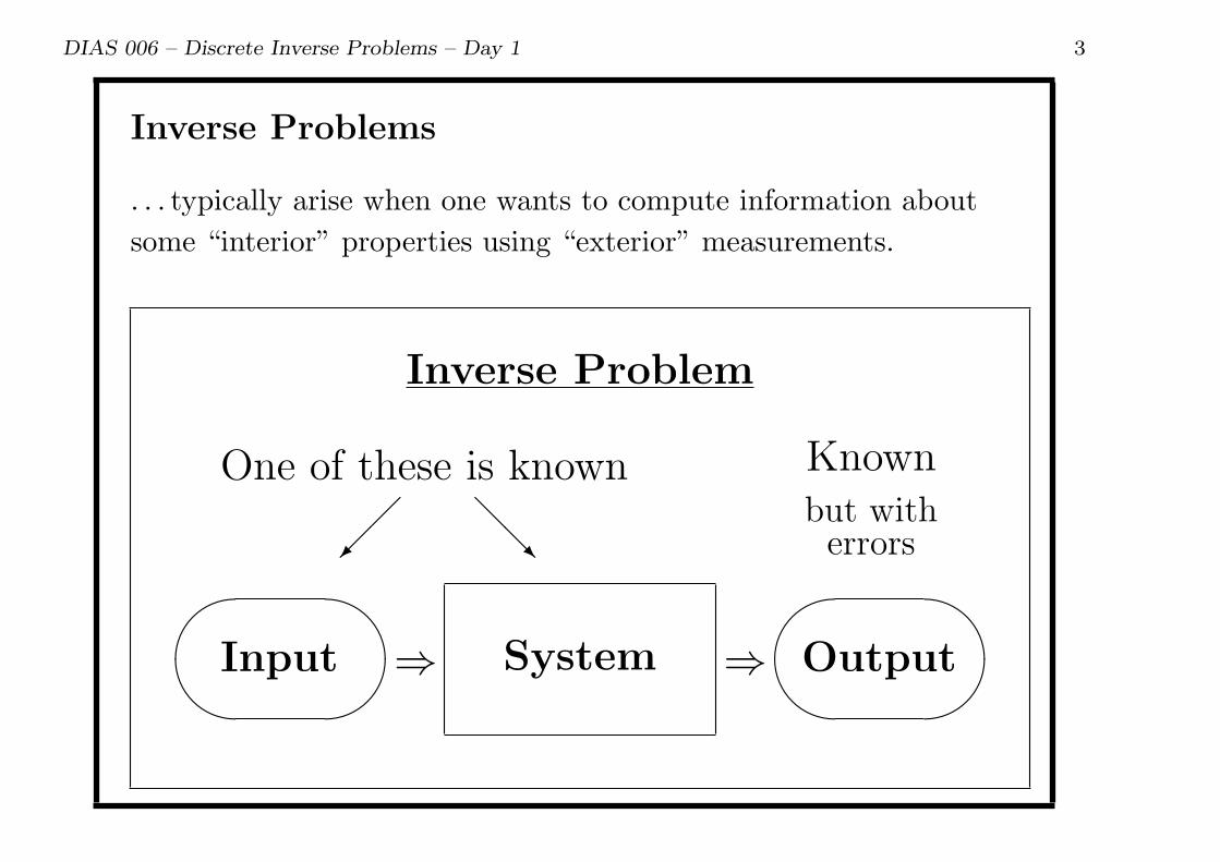
Inverse Problems

. . . typically arise when one wants to compute information about

some “interior” properties using “exterior” measurements.

System

'&

$%Input

'&

$%Output⇒ ⇒

Knownbut witherrors

One of these is known

@@R

Inverse Problem


Inverse Problems: Examples

A quite generic formulation:∫Ω

input × system dΩ = output

Image restoration

scenery → lens → image

Tomography

X-ray source → object → damping

Seismology

seismic wave → layers → reflections


Discrete Ill-Posed Problems

Our generic ill-posed problem:

A Fredholm integral equation of the first kind∫ 1

0

K(s, t) f(t) dt = g(s) , 0 ≤ s ≤ 1 .

Definition of a discrete ill-posed problem (DIP):

1. a square or over-determined system of linear algebraic

equations

Ax = b or minx

∥Ax− b∥2

2. whose coefficient matrix A has a huge condition number, and

3. comes from the discretization of an inverse/ill-posed problem.


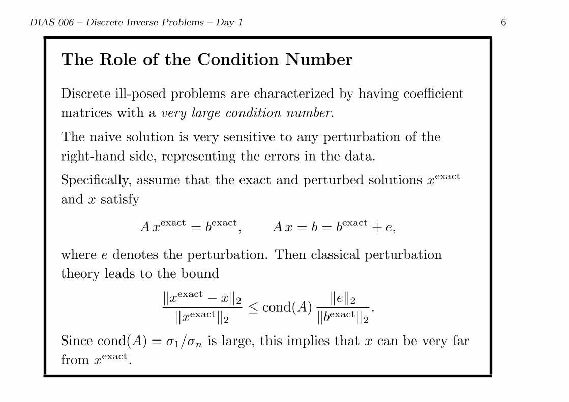
The Role of the Condition Number

Discrete ill-posed problems are characterized by having coefficient

matrices with a very large condition number.

The naive solution is very sensitive to any perturbation of the

right-hand side, representing the errors in the data.

Specifically, assume that the exact and perturbed solutions xexact

and x satisfy

Axexact = bexact, A x = b = bexact + e,

where e denotes the perturbation. Then classical perturbation

theory leads to the bound

∥xexact − x∥2∥xexact∥2

≤ cond(A)∥e∥2

∥bexact∥2.

Since cond(A) = σ1/σn is large, this implies that x can be very far

from xexact.


Computational Issues

The plots below show solutions x to the 64× 64 DIP Ax = b.

0 20 40 60−1

−0.5

0

0.5

1x 10

16 Gaussian elimination

0 20 40 60

0

0.5

1

1.5

2

Truncated SVD

TSVD solution

Exact solution

• Standard numerical methods (x = A\b) produce useless results.

• Specialized methods (this course) produce “reasonable” results.


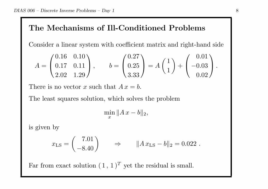
The Mechanisms of Ill-Conditioned Problems

Consider a linear system with coefficient matrix and right-hand side

A =

0.16 0.10

0.17 0.11

2.02 1.29

, b =

0.27

0.25

3.33

= A

(1

1

)+

0.01

−0.03

0.02

.

There is no vector x such that Ax = b.

The least squares solution, which solves the problem

minx

∥Ax− b∥2,

is given by

xLS =

(7.01

−8.40

)⇒ ∥AxLS − b∥2 = 0.022 .

Far from exact solution ( 1 , 1 )T yet the residual is small.


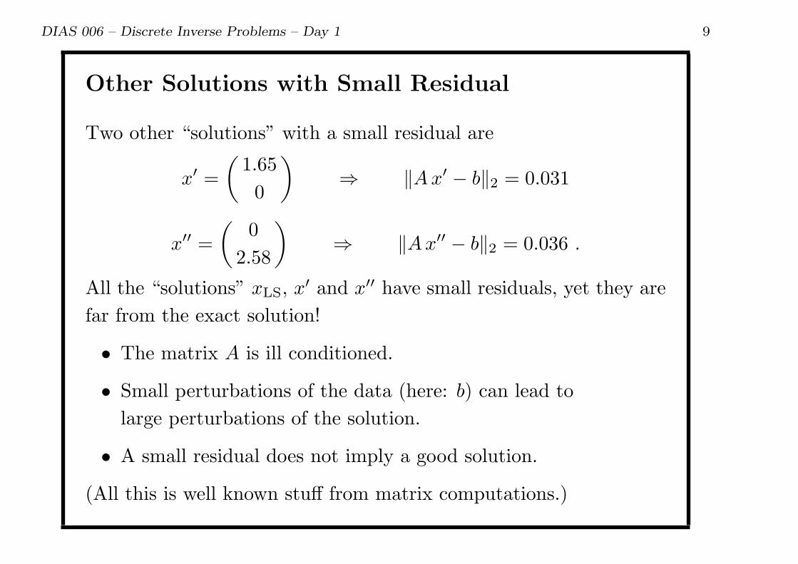
Other Solutions with Small Residual

Two other “solutions” with a small residual are

x′ =

(1.65

0

)⇒ ∥Ax′ − b∥2 = 0.031

x′′ =

(0

2.58

)⇒ ∥Ax′′ − b∥2 = 0.036 .

All the “solutions” xLS, x′ and x′′ have small residuals, yet they are

far from the exact solution!

• The matrix A is ill conditioned.

• Small perturbations of the data (here: b) can lead to

large perturbations of the solution.

• A small residual does not imply a good solution.

(All this is well known stuff from matrix computations.)


Stabilization!

It turns out that we can modify the problem such that the solution

is more stable, i.e., less sensitive to perturbations.

Example: enforce an upper bound on the solution norm ∥x∥2:

minx

∥Ax− b∥2 subject to ∥x∥2 ≤ δ .

The solution xδ depends in a nonlinear way on δ:

x0.1 =

(0.08

0.05

), x1 =

(0.84

0.54

)

x1.385 =

(1.17

0.74

), x10 =

(6.51

−7.60

).

By supplying the correct additional information we can compute

a good approximate solution.


Inverse Problems → Ill-Conditioned Problems

Whenever we solve an inverse problem on a computer, we face

difficulties because the computational problems are ill conditioned.

The purpose of my lectures are:

1. To explain why ill-conditioned computations always arise when

solving inverse problems.

2. To explain the fundamental “mechanisms” underlying the ill

conditioning.

3. To explain how we can modify the problem in order to stabilize

the solution.

4. To show how this can be done efficiently on a computer.

Regularization methods is at the heart of all this.


Inverse Problems are Ill-Posed Problems

Hadamard’s definition of a well-posed problem (early 20th century):

1. the problem must have a solution,

2. the solution must be unique, and

3. it must depend continuously on data and parameters.

If the problem violates any of these requirements, it is ill posed.

Condition 1 can be fixed by reformulating/redefining the solution.

Condition 2 can be “fixed” by additional requirements to the

solution, e.g., that of minimum norm.

Condition 3 is harder to “fix” because it implies that

• arbitrarily small perturbations of data and parameters can

produce arbitrarily large perturbations of the solution.


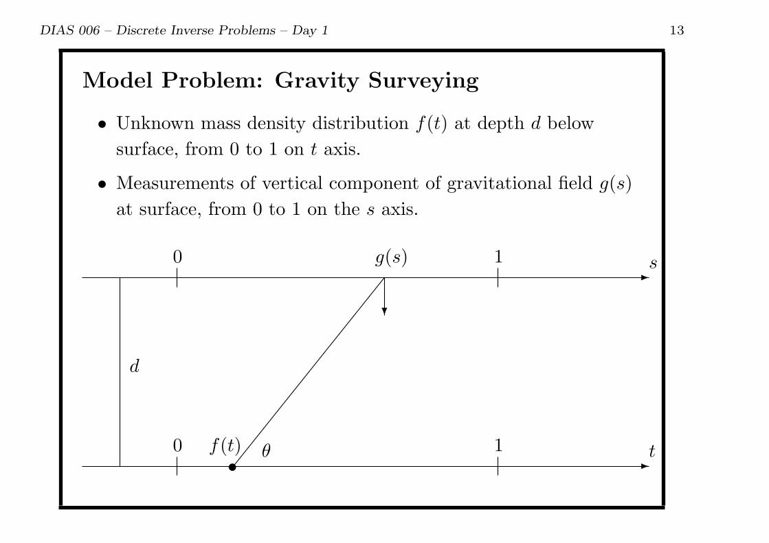
Model Problem: Gravity Surveying

• Unknown mass density distribution f(t) at depth d below

surface, from 0 to 1 on t axis.

• Measurements of vertical component of gravitational field g(s)

at surface, from 0 to 1 on the s axis.

-0 1 s

-0 1 t

d

f(t)•

?

g(s)

θ


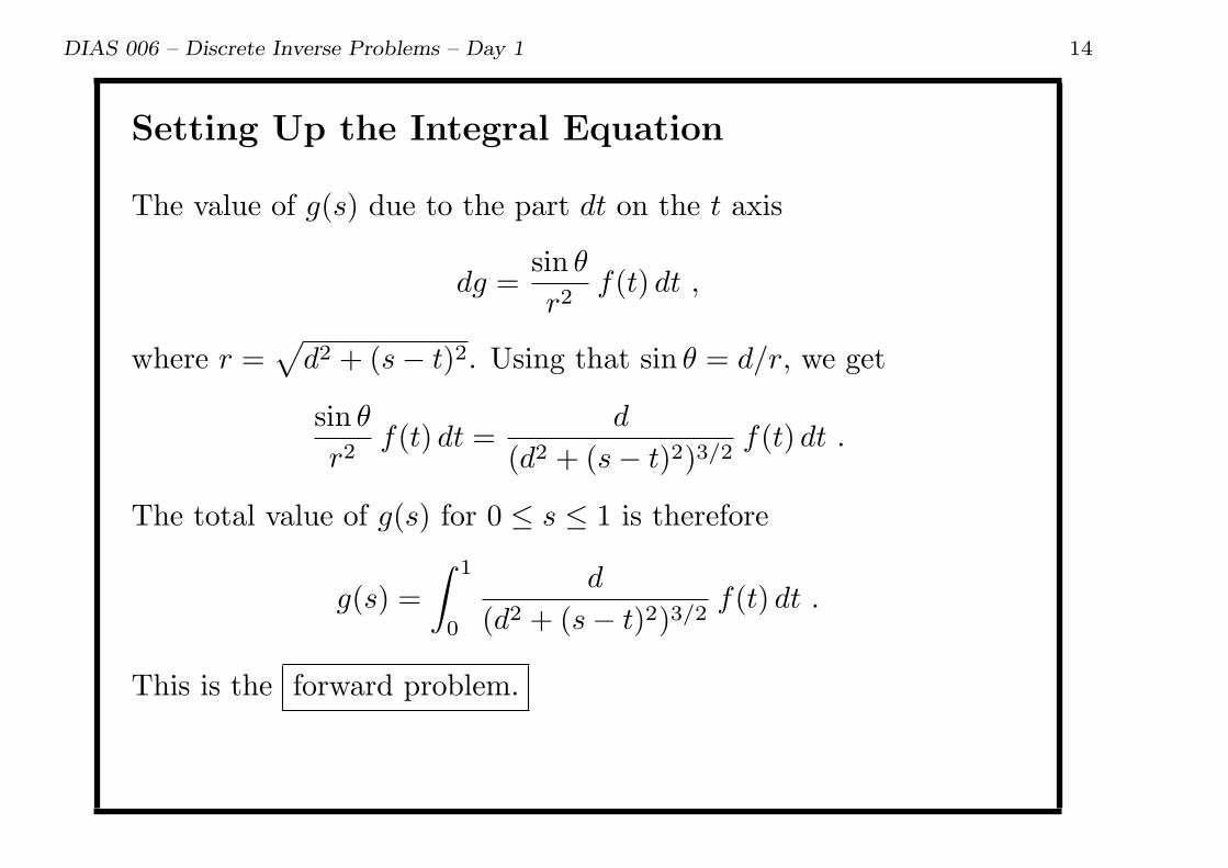
Setting Up the Integral Equation

The value of g(s) due to the part dt on the t axis

dg =sin θ

r2f(t) dt ,

where r =√d2 + (s− t)2. Using that sin θ = d/r, we get

sin θ

r2f(t) dt =

d

(d2 + (s− t)2)3/2f(t) dt .

The total value of g(s) for 0 ≤ s ≤ 1 is therefore

g(s) =

∫ 1

0

d

(d2 + (s− t)2)3/2f(t) dt .

This is the forward problem.


Our Integral Equation

Fredholm integral equation of the first kind:∫ 1

0

d

(d2 + (s− t)2)3/2f(t) dt = g(s) , 0 ≤ s ≤ 1 .

The kernel K, which represents the model, is

K(s, t) = h(s− t) =d

(d2 + (s− t)2)3/2,

and the right-hand side g is what we are able to measure.

From K and g we want to compute f , i.e., an inverse problem.


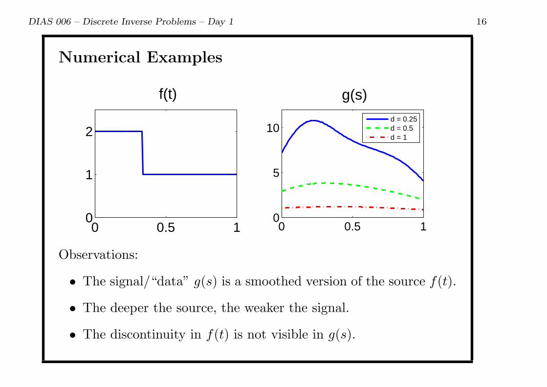
Numerical Examples

0 0.5 10

1

2

f(t)

0 0.5 10

5

10

g(s)

d = 0.25d = 0.5d = 1

Observations:

• The signal/“data” g(s) is a smoothed version of the source f(t).

• The deeper the source, the weaker the signal.

• The discontinuity in f(t) is not visible in g(s).


Fredholm Integral Equations of the First Kind

Our generic inverse problem:∫ 1

0

K(s, t) f(t) dt = g(s), 0 ≤ s ≤ 1 .

Here, the kernel K(s, t) and the right-hand side g(s) are known

functions, while f(t) is the unknown function.

In multiple dimensions, this equation takes the form∫Ωt

K(s, t) f(t) dt = g(s), s ∈ Ωs .

An important special case: K(s, t) = h(s− t) → deconvolution:∫ 1

0

h(s− t) f(t) dt = g(s), 0 ≤ s ≤ 1

(and similarly in more dimensions).


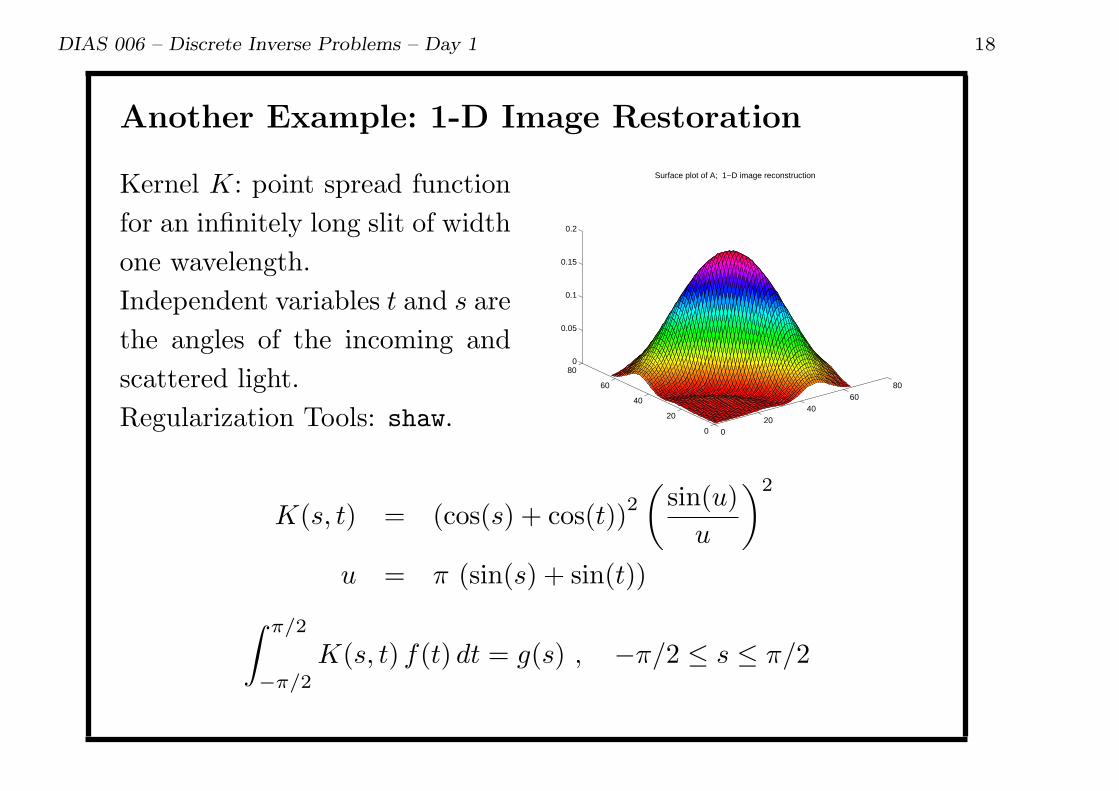
Another Example: 1-D Image Restoration

Kernel K: point spread function

for an infinitely long slit of width

one wavelength.

Independent variables t and s are

the angles of the incoming and

scattered light.

Regularization Tools: shaw.0

2040

6080

0

20

40

60

800

0.05

0.1

0.15

0.2

Surface plot of A; 1−D image reconstruction

K(s, t) = (cos(s) + cos(t))2

(sin(u)

u

)2

u = π (sin(s) + sin(t))∫ π/2

−π/2

K(s, t) f(t) dt = g(s) , −π/2 ≤ s ≤ π/2


Yet Another Example: Second Derivative

Kernel K: Green’s function for

the second derivative

K(s, t) =

s(t− 1) , s < t

t(s− 1) , s ≥ t

0

0.5

1

0

0.2

0.4

0.6

0.8

1−0.25

−0.2

−0.15

−0.1

−0.05

0

t

Plot of K(s,t) − second derivate problem

s

Regularization Tools: deriv2.

Not differentiable across the line t = s.∫ 1

0

K(s, t) f(t) dt = g(s) , 0 ≤ s ≤ 1

Solution:

f(t) = g′′(t) , 0 ≤ t ≤ 1 .


The Riemann-Lebesgue Lemma

Consider the function

f(t) = sin(2πp t) , p = 1, 2, . . .

then for p → ∞ and “arbitrary” K we have

g(s) =

∫ 1

0

K(s, t) f(t) dt → 0 .

Smoothing: high frequencies are damped in the mapping f 7→ g.

Hence, the mapping from g to f must amplify the high frequencies.

Therefore we can expect difficulties when trying to reconstruct

f from noisy data g.


Illustration of the Riemann-Lebesgue Lemma

Gravity problem with f(t) = sin(2πp t), p = 1, 2, 4, and 8.

0 0.5 1−1

−0.5

0

0.5

1

fp(t)

0 0.5 1−1

−0.5

0

0.5

1

gp(s)

p = 1p = 2p = 4p = 8

Higher frequencies are dampen more than low frequencies.


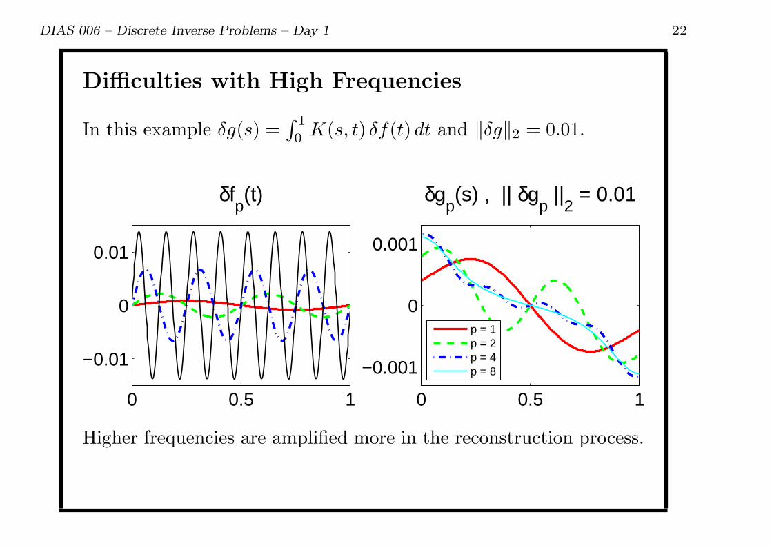
Difficulties with High Frequencies

In this example δg(s) =∫ 1

0K(s, t) δf(t) dt and ∥δg∥2 = 0.01.

0 0.5 1

−0.01

0

0.01

δfp(t)

0 0.5 1

−0.001

0

0.001

δgp(s) , || δg

p ||

2 = 0.01

p = 1p = 2p = 4p = 8

Higher frequencies are amplified more in the reconstruction process.


Why do We Care?

Why bother about these (strange) issues?

• Ill-posed problems model a variety of real applications:

– Medical imaging (brain scanning, etc.)

– Geophysical prospecting (search for oil, land-mines, etc.)

– Image deblurring (astronomy, CSIa, etc.)

– Deconvolution of instrument’s response.

• We can only hope to compute useful solutions to these

problems if we fully understand their inherent difficulties . . .

• and how these difficulties carry over to the discretized problems

involved in a computer solution,

• and how to deal with them in a satisfactory way.aCrime Scene Investigation.


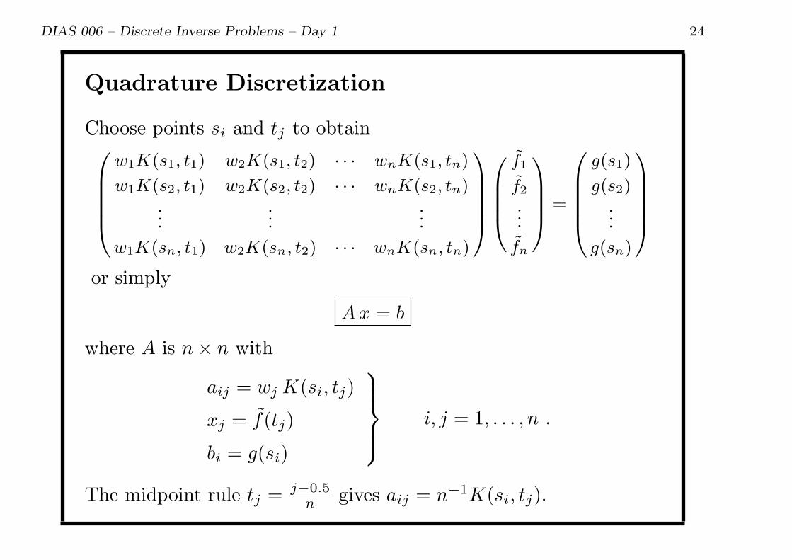
Quadrature Discretization

Choose points si and tj to obtainw1K(s1, t1) w2K(s1, t2) · · · wnK(s1, tn)

w1K(s2, t1) w2K(s2, t2) · · · wnK(s2, tn)...

......

w1K(sn, t1) w2K(sn, t2) · · · wnK(sn, tn)

f1

f2...

fn

=

g(s1)

g(s2)...

g(sn)

or simply

Ax = b

where A is n× n with

aij = wj K(si, tj)

xj = f(tj)

bi = g(si)

i, j = 1, . . . , n .

The midpoint rule tj =j−0.5

n gives aij = n−1K(si, tj).


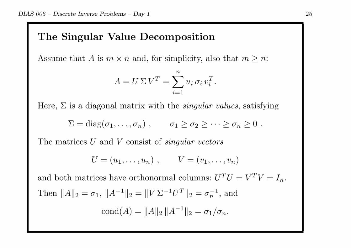
The Singular Value Decomposition

Assume that A is m× n and, for simplicity, also that m ≥ n:

A = U ΣV T =n∑

i=1

ui σi vTi .

Here, Σ is a diagonal matrix with the singular values, satisfying

Σ = diag(σ1, . . . , σn) , σ1 ≥ σ2 ≥ · · · ≥ σn ≥ 0 .

The matrices U and V consist of singular vectors

U = (u1, . . . , un) , V = (v1, . . . , vn)

and both matrices have orthonormal columns: UTU = V TV = In.

Then ∥A∥2 = σ1, ∥A−1∥2 = ∥V Σ−1UT ∥2 = σ−1n , and

cond(A) = ∥A∥2 ∥A−1∥2 = σ1/σn.


SVD Software for Dense Matrices

Software package Subroutine

ACM TOMS HYBSVD

EISPACK SVD

IMSL LSVRR

LAPACK GESVD

LINPACK SVDC

NAG F02WEF

Numerical Recipes SVDCMP

Matlab svd, ssvd

Reg. Tools csvd

Complexity of SVD algorithms: O(mn2).


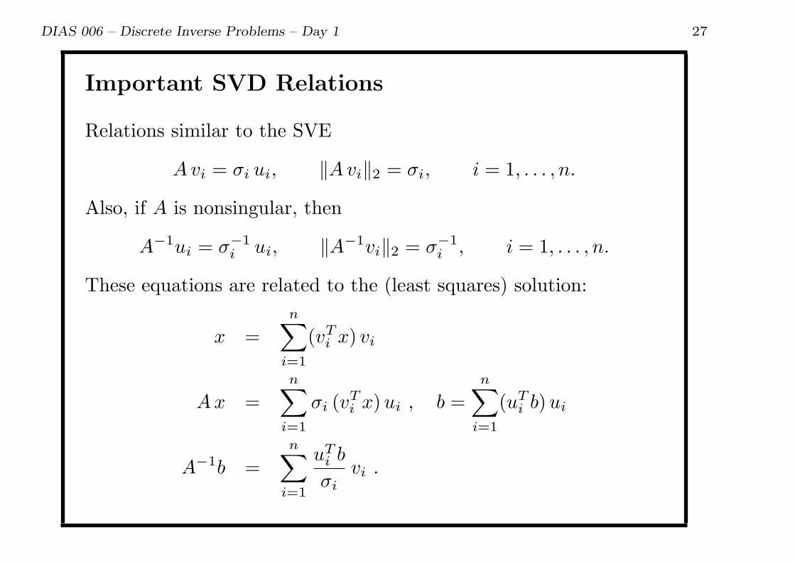
Important SVD Relations

Relations similar to the SVE

Avi = σi ui, ∥Avi∥2 = σi, i = 1, . . . , n.

Also, if A is nonsingular, then

A−1ui = σ−1i ui, ∥A−1vi∥2 = σ−1

i , i = 1, . . . , n.

These equations are related to the (least squares) solution:

x =

n∑i=1

(vTi x) vi

Ax =n∑

i=1

σi (vTi x)ui , b =

n∑i=1

(uTi b)ui

A−1b =n∑

i=1

uTi b

σivi .


What the SVD Looks Like

The following figures show the SVD of the 64× 64 matrix A,

computed by means of csvd from Regularization Tools:

>> help csvd

CSVD Compact singular value decomposition.

s = csvd(A)

[U,s,V] = csvd(A)

[U,s,V] = csvd(A,’full’)

Computes the compact form of the SVD of A:

A = U*diag(s)*V’,

where

U is m-by-min(m,n)

s is min(m,n)-by-1

V is n-by-min(m,n).

If a second argument is present, the full U and V are returned.


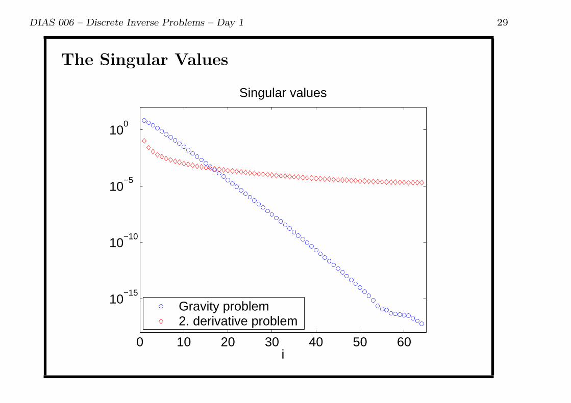
The Singular Values

0 10 20 30 40 50 60

10−15

10−10

10−5

100

i

Singular values

Gravity problem2. derivative problem


The Left and Right Singular Vectors

0 20 40 60−0.2

0

0.2

u1

0 20 40 60−0.2

0

0.2

u2

0 20 40 60−0.2

0

0.2

u3

0 20 40 60−0.2

0

0.2

u4

0 20 40 60−0.2

0

0.2

u5

0 20 40 60−0.2

0

0.2

u6

0 20 40 60−0.2

0

0.2

u7

0 20 40 60−0.2

0

0.2

u8

0 20 40 60−0.2

0

0.2

u9


Some Observations

• The singular values decay gradually to zero.

• No gap in the singular value spectrum.

• Condition number cond(A) = “∞.”

• Singular vectors have more oscillations as i increases.

• In this problem, # sign changes = i− 1.

The following pages: Picard plots with increasing noise.


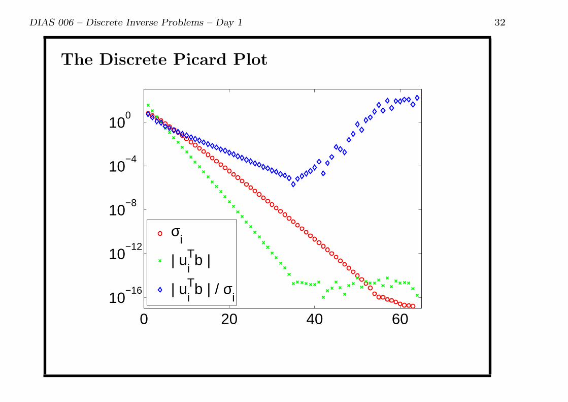
The Discrete Picard Plot

0 20 40 6010

−16

10−12

10−8

10−4

100

σi

| uiTb |

| uiTb | / σ

i


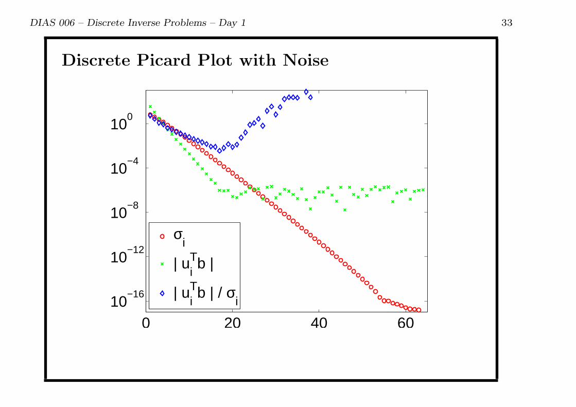
Discrete Picard Plot with Noise

0 20 40 6010

−16

10−12

10−8

10−4

100

σi

| uiTb |

| uiTb | / σ

i


Discrete Picard Plot – More Noise

0 12 24

10−4

10−2

100

102

σi

| uiTb |

| uiTb | / σ

i


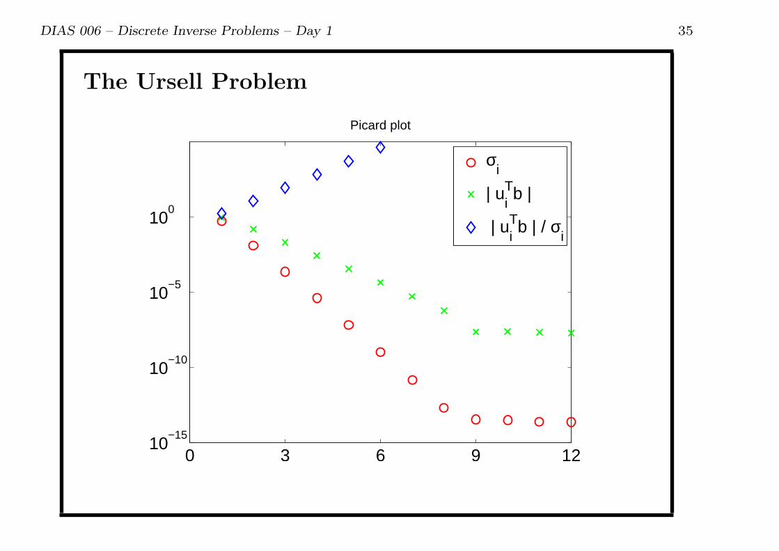
The Ursell Problem

0 3 6 9 1210

−15

10−10

10−5

100

Picard plot

σi

| uiTb |

| uiTb | / σ

i


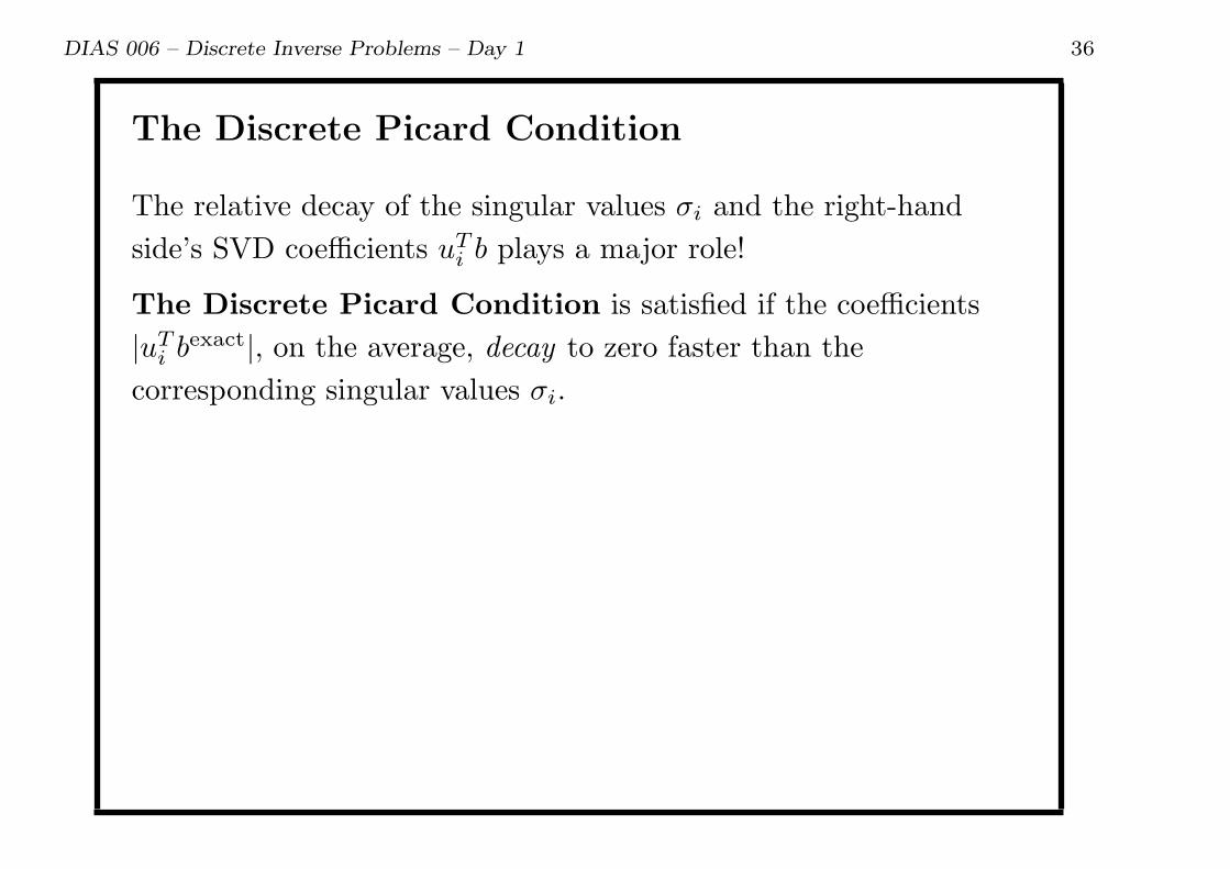
The Discrete Picard Condition

The relative decay of the singular values σi and the right-hand

side’s SVD coefficients uTi b plays a major role!

The Discrete Picard Condition is satisfied if the coefficients

|uTi b

exact|, on the average, decay to zero faster than the

corresponding singular values σi.


Noisy Problems

Real problems have noisy data! Recall that we consider problems

Ax = b or minx ∥Ax− b∥2

with a very ill-conditioned coefficient matrix A,

cond(A) ≫ 1.

Noise model:

b = bexact + e, where bexact = Axexact .

The ingredients:

• xexact is the exact (and unknown) solution,

• bexact is the exact data, and

• the vector e represents the noise in the data.


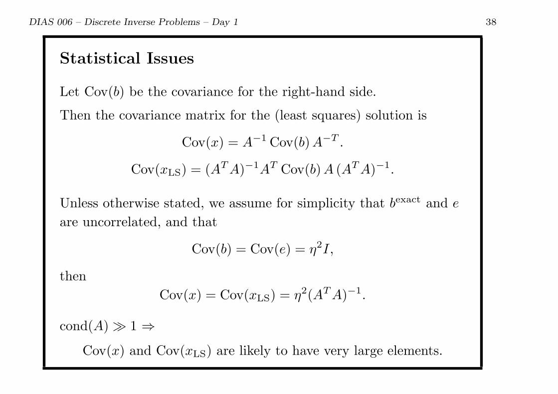
Statistical Issues

Let Cov(b) be the covariance for the right-hand side.

Then the covariance matrix for the (least squares) solution is

Cov(x) = A−1 Cov(b)A−T .

Cov(xLS) = (ATA)−1AT Cov(b)A (ATA)−1.

Unless otherwise stated, we assume for simplicity that bexact and e

are uncorrelated, and that

Cov(b) = Cov(e) = η2I,

then

Cov(x) = Cov(xLS) = η2(ATA)−1.

cond(A) ≫ 1 ⇒

Cov(x) and Cov(xLS) are likely to have very large elements.


The Story So Far

• Inverse problems are ill posed: they are very sensitive to

perturbations of the data.

• Discretization → a matrix problem Ax = b.

• The singular value decomposition, SVD, is a powerful tool to

analyze discrete inverse problems.

• The discrete Picard condition gives information about the

existence of a meaningful solution.

• The troublemakers: the large condition number cond(A) and

the noise in the right-hand side.


Matrix Problems

From now on, the coefficient matrix A is allowed to have more rows

than columns, i.e.,

A ∈ Rm×n with m ≥ n.

For m > n it is natural to consider the least squares problem

minx ∥Ax− b∥2.

When we say “naive solution” we either mean the solution A−1b

(when m = n) or the least squares solution (when m > n).

We emphasize the convenient fact that the naive solution has

precisely the same SVD expansion in both cases:

xnaive =n∑

i=1

uTi b

σivi.


Naive Solutions are Useless

0 0.5 1−0.1

0

0.1

0.2cond(A) = 4979, ||e||

2 = 5e−5

0 0.5 10

0.5

1

1.5

cond(A) = 3.4e9, ||e||2 = 1e−7

0 0.5 10

0.5

1

1.5

cond(A) = 2.5e16, ||e||2 = 0

Exact solutions (blue smooth lines) together with the naive

solutions (jagged green lines) to two test problems.

Left: deriv2 with n = 64.

Middle and right: gravity with n = 32 and n = 53.


Need For Regularization

Discrete ill-posed problems are characterized by having coefficient

matrices with a very large condition number.

The naive solution is very sensitive to any perturbation of the

right-hand side, representing the errors in the data.

Specifically, assume that the exact and perturbed solutions xexact

and x satisfy

Axexact = bexact, A x = b = bexact + e,

where e denotes the perturbation. Then classical perturbation

theory leads to the bound

∥xexact − x∥2∥xexact∥2

≤ cond(A)∥e∥2

∥bexact∥2.

Since cond(A) = σ1/σn is large, this implies that x can be very far

from xexact.


Rn = spanv1, . . . , vn Rm = spanu1, . . . , um

•Exact sol.: xexact

•bexact = Axexact

-

b = bexact + e@@R

+Naive sol.: xnaive

⋆xk (TSVD)

∗ xλ (Tikhonov)


Regularization Methods → Spectral Filtering

Almost all the regularization methods treated in this course

produce solutions which can be expressed as a filtered SVD

expansion of the form

xreg =

n∑i=1

φiuTi b

σivi,

where φi are the filter factors associated with the method.

These methods are called spectral filtering methods because the

SVD basis can be considered as a spectral basis.


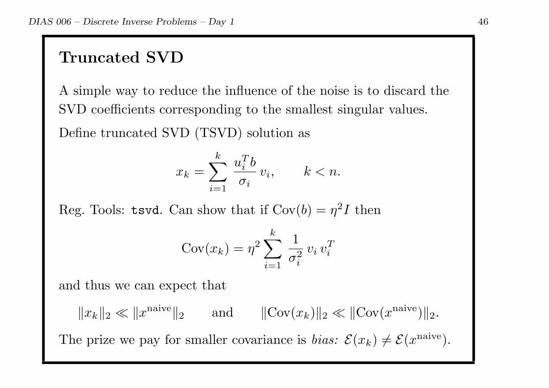
Truncated SVD

A simple way to reduce the influence of the noise is to discard the

SVD coefficients corresponding to the smallest singular values.

Define truncated SVD (TSVD) solution as

xk =k∑

i=1

uTi b

σivi, k < n.

Reg. Tools: tsvd. Can show that if Cov(b) = η2I then

Cov(xk) = η2k∑

i=1

1

σ2i

vi vTi

and thus we can expect that

∥xk∥2 ≪ ∥xnaive∥2 and ∥Cov(xk)∥2 ≪ ∥Cov(xnaive)∥2.

The prize we pay for smaller covariance is bias: E(xk) = E(xnaive).


Truncated SVD Solutions

0 32 640

0.5

1

k = 2

0 32 640

0.5

1

k = 4

0 32 640

0.5

1

k = 6

0 32 640

0.5

1

k = 8

0 32 640

0.5

1

k = 10

0 32 640

0.5

1

k = 12

0 32 640

0.5

1

k = 14

0 32 640

0.5

1

k = 16

0 32 640

0.5

1

Exact solution


The Truncation Parameter

Note: the truncation parameter k in

xk =k∑

i=1

uTi b

σivi

is dictated by the coefficients uTi b, not the singular values!

Basically we should choose k as the index i where |uTi b| start to

“level off” due to the noise.


Discrete Tikhonov Regularization

Minimization of the residual takes the form

minx

∥Ax− b∥2 , A ∈ Rm×n ,

where A and b are obtained by discretization of the integral eq.

We also introduce a smoothing norm

Ω(x) = ∥x∥2

that penalizes a large solution norm.

The resulting discrete Tikhonov problem is thus

minx∥Ax− b∥22 + λ2 ∥x∥22

.

Regularization Tools: tikhonov.


Tikhonov Solutions

0 32 640

0.5

1

λ = 10

0 32 640

0.5

1

λ = 2.6827

0 32 640

0.5

1

λ = 0.71969

0 32 640

0.5

1

λ = 0.19307

0 32 640

0.5

1

λ = 0.051795

0 32 640

0.5

1

λ = 0.013895

0 32 640

0.5

1

λ = 0.0037276

0 32 640

0.5

1

λ = 0.001

0 32 640

0.5

1

Exact solution


Efficient Implementation

The original formulation

min∥Ax− b∥22 + λ2 ∥x∥22

.

Two alternative formulations

(ATA+ λ2I)x = AT b

min

∥∥∥∥( A

λ I

)x−

(b

0

)∥∥∥∥2

The first shows that we have a linear problem. The second shows

how to solve it stably:

• treat it as a least squares problem,

• utilize any sparsity or structure.


SVD and Tikhonov Regularization

We can write the discrete Tikhonov solution xλ in terms of the

SVD of A as

xλ =n∑

i=1

σ2i

σ2i + λ2

uTi b

σivi =

n∑i=1

ϕ[λ]i

uTi b

σi.

The filter factors are given by

ϕ[λ]i =

σ2i

σ2i + λ2

,

and their purpose is to dampen the components in the solution

corresponding to small σi.


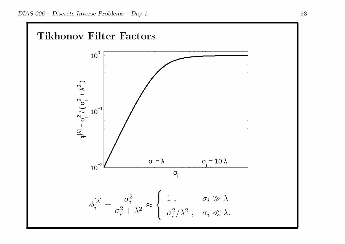
Tikhonov Filter Factors

10−2

10−1

100

σi

φ[λ] =

σi2 /

( σ i2 +

λ2 )

σi = λ σ

i = 10 λ

ϕ[λ]i =

σ2i

σ2i + λ2

≈

1 , σi ≫ λ

σ2i /λ

2 , σi ≪ λ.


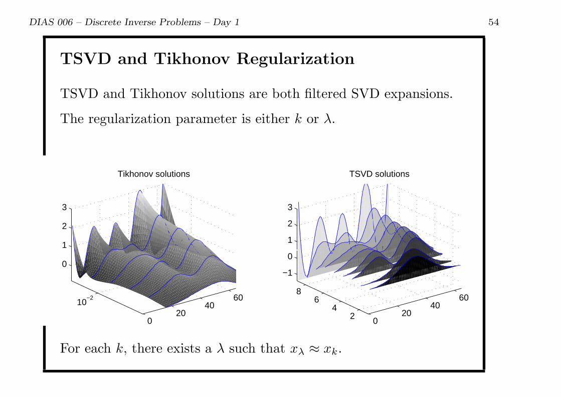
TSVD and Tikhonov Regularization

TSVD and Tikhonov solutions are both filtered SVD expansions.

The regularization parameter is either k or λ.

020

406010

−2

0

1

2

3

Tikhonov solutions

020

4060

24

68

−1

0

1

2

3

TSVD solutions

For each k, there exists a λ such that xλ ≈ xk.


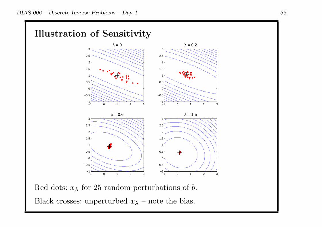
Illustration of Sensitivity

−1 0 1 2 3−1

−0.5

0

0.5

1

1.5

2

2.5

3λ = 0

−1 0 1 2 3−1

−0.5

0

0.5

1

1.5

2

2.5

3λ = 0.2

−1 0 1 2 3−1

−0.5

0

0.5

1

1.5

2

2.5

3λ = 0.6

−1 0 1 2 3−1

−0.5

0

0.5

1

1.5

2

2.5

3λ = 1.5

Red dots: xλ for 25 random perturbations of b.

Black crosses: unperturbed xλ – note the bias.


The L-Curve for Tikhonov Regularization

Plot of ∥xλ∥2 versus ∥Axλ − b∥2 in log-log scale.

10−1

100

101

100

101

102

103

Residual norm || A xλ − b ||2

Sol

utio

n no

rm ||

xλ ||

2

λ = 1λ = 0.1

λ = 1e−4

λ = 1e−5


The Story So Far

• The purpose of regularization is to suppress the influence of the

noise, while still achieving an approximation to the exact

solution.

• This is done by filtering the SVD components, e.g., by

– a sharp filter → truncated SVD

– a smooth filter → Tikhonov.

This works because it is mainly the “high-frequency” SVD

components that are affected by the noise.

• The discrete Picard condition ensures that the “low-frequency”

SVD components are approximated well.

• The L-curve provides a means for displaying the tradeoff

between solution norm and residual norm (over- versus

under-smoothing).


Choosing the Regularization Parameter

At our disposal: several regularization methods, based on filtering

of the SVD components.

Often fairly straightforward to “eyeball” a good TSVD truncation

parameter from the Picard plot.

Need: a reliable and automated technique for choosing the regu-

larization parameter, such as k (for TSVD) or λ (for Tikhonov).

1. Perspectives on regularization

2. The discrepancy principle

3. Generalized cross validation (GCV)

4. The L-curve criterion

5. The NCP method


Once Again: Tikhonov Regularization

Focus on Tikhonov regularization; the ideas carry over to many

other methods.

Recall that the Tikhonov solution xλ solves the problem

minx

∥Ax− b∥22 + λ2∥x∥22

,

and that it is formally given by

xλ = (ATA+ λ2I)−1AT b = A#λ b,

where A#λ = (ATA+ λ2I)−1AT is a “regularized inverse.”

Our noise model

b = bexact + e

where bexact = Axexact and e is the error.


Classical and Pragmatic Parameter-Choice

Assume we are given the problem Ax = b with b = bexact + e, and

that we have a strategy for choosing the regularization parameter λ

as a function of the “noise level” ∥e∥2.

Then classical parameter-choice analysis is concerned with the

convergence rates of

xλ → xexact as ∥e∥2 → 0 and λ → 0 .

The typical situation in practice is different:

• The norm ∥e∥2 is not known, and

• the errors are fixed (not practical to repeat the measurements).

The pragmatic approach to choosing the regularization parameter

is based on the forward/prediction error, or the backward error.


An Example (Image of Io, a Moon of Saturn)

Exact Blurred

λ too large λ ≈ ok λ too small


Perspectives on Regularization

Problem formulation: balance fit (residual) and size of solution.

xλ = argmin∥Ax− b∥22 + λ2∥x∥22

Cannot be used for choosing λ.

Forward error: balance regularization and perturbation errors.

xexact − xλ = xexact −A#λ (b

exact + e)

=(I −A#

λ A)xexact −A#

λ e .

Backward/prediction error: balance residual and perturbation.

bexact −Axλ = bexact −AA#λ (b

exact + e)

=(I −AA#

λ

)bexact −AA#

λ e .


More About the Forward Error

The forward error in the SVD basis:

xexact − xλ = xexact − V Φ[λ] Σ−1 UT b

= xexact − V Φ[λ] Σ−1 UTAxexact − V Φ[λ] Σ−1 UT e

= V(I − Φ[λ]

)V Txexact − V Φ[λ] Σ−1 UT e.

The first term is the regularization error:

∆xbias = V(I − Φ[λ]

)V Txexact =

n∑i=1

(1− φ

[λ]i

)(vTi x

exact) vi,

and we recognize this as (minus) the bias term.

The second error term is the perturbation error:

∆xpert = V Φ[λ] Σ−1 UT e.


Regularization and Perturbation Errors – TSVD

For TSVD solutions, the regularization and perturbation errors

take the form

∆xbias =n∑

i=k+1

(vTi xexact) vi, ∆xpert =

k∑i=1

uTi e

σivi.

We use the truncation parameter k to prevent the perturbation

error from blowing up (due to the division by the small singular

values), at the cost of introducing bias in the regularized solution.

A “good” choice of the truncation parameter k should balance

these two components of the forward error (see next slide).

The behavior of ∥xk∥2 and ∥Axk − b∥2 is closely related to these

errors – see the analysis in §5.1.


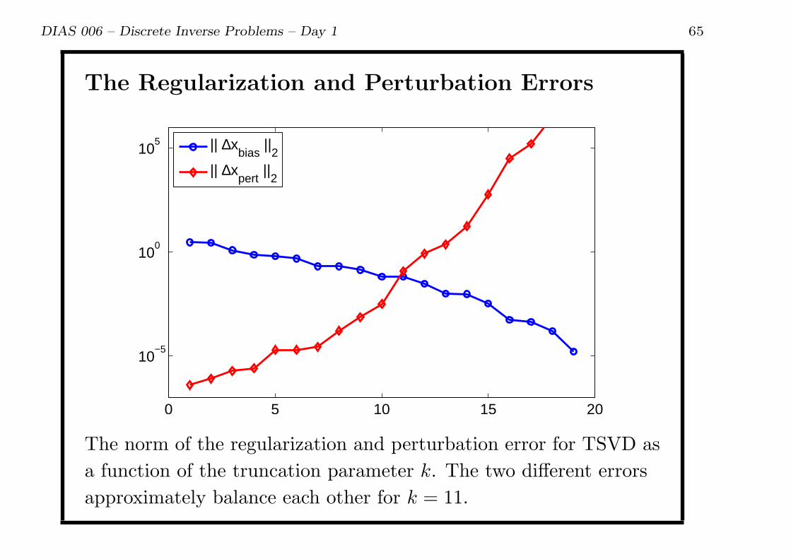
The Regularization and Perturbation Errors

0 5 10 15 20

10−5

100

105

|| ∆xbias

||2

|| ∆xpert

||2

The norm of the regularization and perturbation error for TSVD as

a function of the truncation parameter k. The two different errors

approximately balance each other for k = 11.


The TSVD Residual

Let kη denote the index that marks the transition between

decaying and flat coefficients |uTi b|.

Due to the discrete Picard condition, the coefficients |uTi b|/σi will

also decay, on the average, for all i < kη.

k < kη : ∥Axk − b∥22 ≈kη∑

i=k+1

(uTi b)

2 +(n− kη)η2 ≈

kη∑i=k+1

(uTi b

exact)2

k > kη : ∥Axk − b∥22 ≈ (n− k) η2.

For k < kη the residual norm decreases steadily with k.

For k > kη it decreases much more slowly.

The transition between the two types of behavior occurs at k = kη

when the regularization and perturbation errors are balanced.


The Discrepancy Principle

Recall that E(∥e∥2) ≈ n1/2η.

We should ideally choose k such that ∥Axk − b∥2 ≈ (n− k)1/2 η.

The discrepancy principle (DP) seeks to combine this:

Assume we have an upper bound δe for the noise level, then solve

∥Axλ − b∥2 = τ δe , where ∥e∥2 ≤ δe

and τ is some parameter τ = O(1). See next slide.

A statistician’s point of view. Write xλ = A#λ b and assume

Cov(b) = η2I; choose the λ that solves

∥Axλ − b∥2 =(∥e∥22 − η2 trace(AA#

λ ))1/2

.

Note that the right-hand side now depends on λ.

Both versions of the DP are very sensitive to the estimate δe.


Illustration of the Discrepancy Principle

0 5 10 15 2010

−7

10−6

10−5

10−4

10−3

k

|| A xk − b ||

2

|| e ||2

(n−kη)1/2 η

The choice ∥Axk − b∥2 ≈ (n− kη)1/2η leads to a too large value of

the truncation parameter k, while the more conservative choice

∥Axk − b∥2 ≈ ∥e∥2 leads to a better value of k.


The L-Curve for Tikhonov Regularization

Recall that the L-curve is a log-log-plot of the solution norm

versus the residual norm, with λ as the parameter.

10−1

100

101

100

101

102

103

Residual norm || A xλ − b ||2

Sol

utio

n no

rm ||

xλ ||

2

λ = 1λ = 0.1

λ = 1e−4

λ = 1e−5


Parameter-Choice and the L-Curve

Recall that the L-curve basically consists of two parts.

• A “flat” part where the regularization errors dominates.

• A “steep” part where the perturbation error dominates.

The optimal regularization parameter (in the pragmatic sense)

must lie somewhere near the L-curve’s corner.

The component bexact dominates when λ is large:

∥xλ∥2 ≈ ∥xexact∥2 (constant)

∥b−Axλ∥2 increases with λ.

The error e dominates when λ is small:

∥xλ∥2 increases with λ−1

∥b−Axλ∥2 ≈ ∥e∥2 (constant.)


The L-Curve Criterion

The flat and the steep parts of the L-curve represent solutions that

are dominated by regularization errors and perturbation errors.

• The balance between these two errors must occur near the

L-curve’s corner.

• The two parts – and the corner – are emphasized in log-log

scale.

• Log-log scale is insensitive to scalings of A and b.

An operational definition of the corner is required.

Write the L-curve as

(log ∥Axλ − b∥2 , log ∥xλ∥2)

and seek the point with maximum curvature.


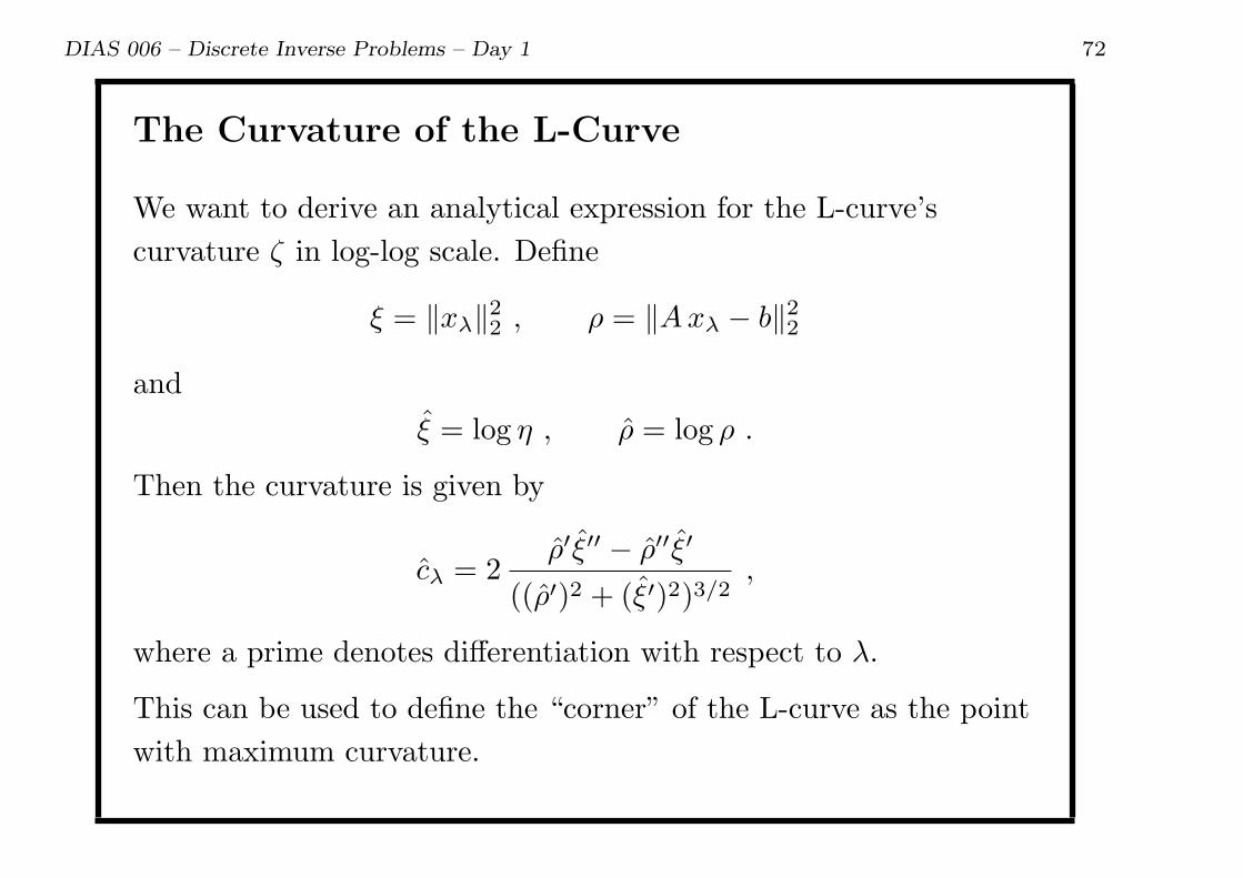
The Curvature of the L-Curve

We want to derive an analytical expression for the L-curve’s

curvature ζ in log-log scale. Define

ξ = ∥xλ∥22 , ρ = ∥Axλ − b∥22

and

ξ = log η , ρ = log ρ .

Then the curvature is given by

cλ = 2ρ′ξ′′ − ρ′′ξ′

((ρ′)2 + (ξ′)2)3/2,

where a prime denotes differentiation with respect to λ.

This can be used to define the “corner” of the L-curve as the point

with maximum curvature.


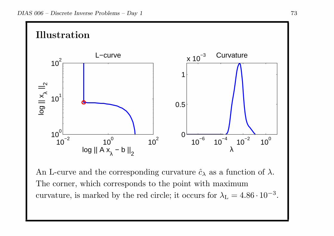
Illustration

10−2

100

102

100

101

102

L−curve

log || A xλ − b ||2

log

|| x λ ||

2

10−6

10−4

10−2

100

0

0.5

1

x 10−3

λ

Curvature

An L-curve and the corresponding curvature cλ as a function of λ.

The corner, which corresponds to the point with maximum

curvature, is marked by the red circle; it occurs for λL = 4.86 · 10−3.


The Prediction Error

A different kind of goal: find the value of λ or k such that Axλ or

Axk predicts the exact data bexact = Axexact as well as possible.

We split the analysis in two cases, depending on k:

k < kη : ∥Axk − bexact∥22 ≈ k η2 +

kη∑i=k+1

(uTi b

exact)2

k > kη : ∥Axk − bexact∥22 ≈ k η2.

For k < kη the norm of the prediction error decreases with k.

For k > kη the norm increases with k.

The minimum arises near the transition, i.e., for k ≈ kη. Hence it

makes good sense to search for the regularization parameter that

minimizes the prediction error. But bexact is unknown . . .


(Ordinary) Cross-Validation

Leave-one-out approach:

skip ith element bi and predict this element.

A(i) = A([1: i− 1, i+ 1:m], : )

b(i) = b([1: i− 1, i+ 1:m])

x(i)λ =

(A(i)

)#λb(i) (Tikh. sol. to reduced problem)

bpredicti = A(i, : )x(i)λ (prediction of “missing” element.)

The optimal λ minimizes the quantity

C(λ) =m∑i=1

(bi − bpredicti

)2.

But λ is hard to compute, and depends on the ordering of the data.


Generalized Cross-Validation

Want a scheme for which λ is independent of any orthogonal

transformation of b (incl. a permutation of the elements).

Minimize the GCV function

G(λ) =∥Axλ − b∥22

trace(Im −AA#λ )

2

where

trace(Im −AA#λ ) = m−

n∑i=1

φ[λ]i .

Easy to compute the trace term when the SVD is available.

For TSVD the trace term is particularly simple:

m−n∑

i=1

φ[λ]i = m− k .


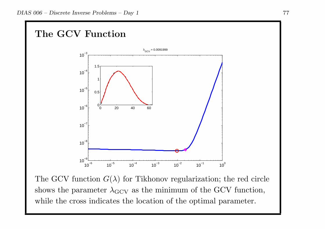
The GCV Function

10−6

10−5

10−4

10−3

10−2

10−1

100

10−9

10−8

10−7

10−6

10−5

10−4

10−3

λGCV

= 0.0091999

0 20 40 600

0.5

1

1.5

The GCV function G(λ) for Tikhonov regularization; the red circle

shows the parameter λGCV as the minimum of the GCV function,

while the cross indicates the location of the optimal parameter.


Occasional Failure

Occasional failure leading to a too small λ; more pronounced for

correlated noise.

10−6

10−5

10−4

10−3

10−2

10−1

100

10−9

10−8

10−7

10−6

10−5

10−4

10−3

λGCV

= 0.00045723

0 20 40 600

0.5

1

1.5


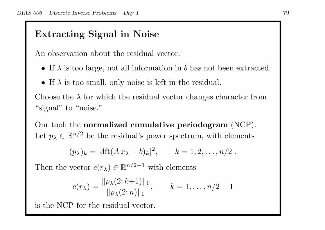
Extracting Signal in Noise

An observation about the residual vector.

• If λ is too large, not all information in b has not been extracted.

• If λ is too small, only noise is left in the residual.

Choose the λ for which the residual vector changes character from

“signal” to “noise.”

Our tool: the normalized cumulative periodogram (NCP).

Let pλ ∈ Rn/2 be the residual’s power spectrum, with elements

(pλ)k = |dft(Axλ − b)k|2, k = 1, 2, . . . , n/2 .

Then the vector c(rλ) ∈ Rn/2−1 with elements

c(rλ) =∥pλ(2: k+1)∥1∥pλ(2:n)∥1

, k = 1, . . . , n/2− 1

is the NCP for the residual vector.


NCP Analysis

0 64 1280

0.5

1White noise

0 64 1280

0.5

1LF noise

0 64 1280

0.5

1HF noise

Left to right: 10 instances of white-noise residuals, 10 instances of

residuals dominated by low-frequency components, and 10

instances of residuals dominated by high-frequency components.

The dashed lines show the Kolmogorov-Smirnoff limits

±1.35 q−1/2 ≈ ±0.12 for a 5% significance level, with q = n/2− 1.


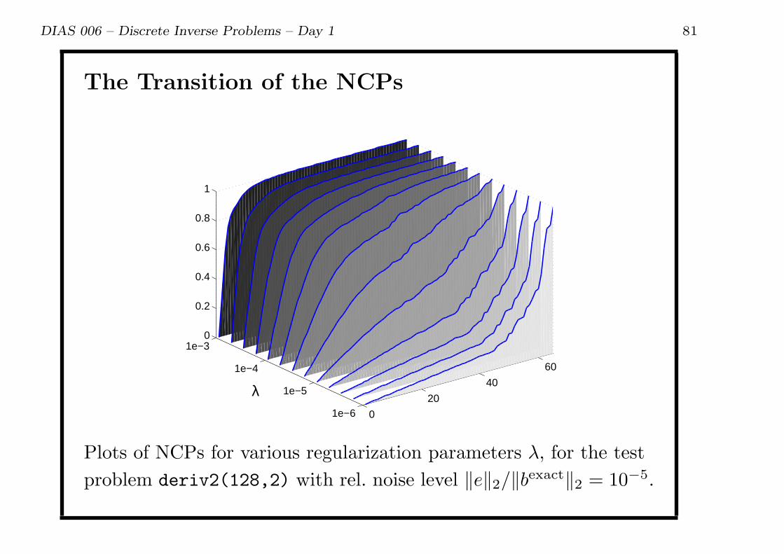
The Transition of the NCPs

0

20

40

60

1e−6

1e−5

1e−4

1e−30

0.2

0.4

0.6

0.8

1

λ

Plots of NCPs for various regularization parameters λ, for the test

problem deriv2(128,2) with rel. noise level ∥e∥2/∥bexact∥2 = 10−5.


Implementation of NCP Criterion

Two ways to implement a pragmatic NCP criterion.

• Adjust the regularization parameter until the NCP lies solely

within the K-S limits.

• Choose the regularization parameter for which the NCP is

closest to a straight line cwhite = (1/q, 2/q, . . . , 1)T .

The latter is implemented in Regularization Tools.


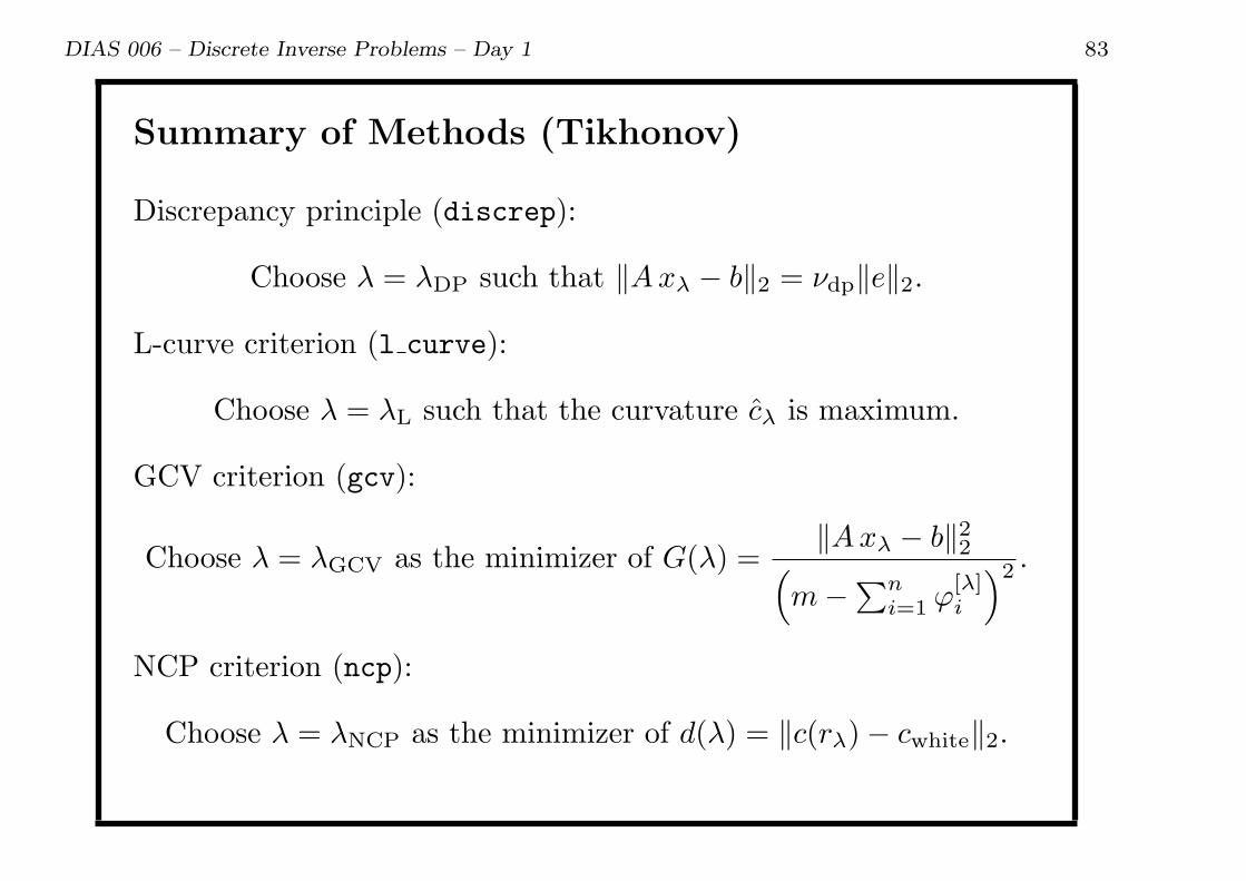
Summary of Methods (Tikhonov)

Discrepancy principle (discrep):

Choose λ = λDP such that ∥Axλ − b∥2 = νdp∥e∥2.

L-curve criterion (l curve):

Choose λ = λL such that the curvature cλ is maximum.

GCV criterion (gcv):

Choose λ = λGCV as the minimizer of G(λ) =∥Axλ − b∥22(

m−∑n

i=1 φ[λ]i

)2 .

NCP criterion (ncp):

Choose λ = λNCP as the minimizer of d(λ) = ∥c(rλ)− cwhite∥2.


Comparison of Methods

To evaluate the performance of the four methods, we need the

optimal regularization parameter λopt:

λopt = argminλ∥xexact − xλ∥2.

This allows us to compute the four ratios

RDP =λDP

λopt, RL =

λL

λopt, RGCV =

λGCV

λopt, RNCP =

λNCP

λopt,

one for each parameter-choice method, and study their

distributions via plots of their histograms (in log scale).

The closer these ratios are to one, the better, so a spiked histogram

located at one is preferable.


First Example: gravity

0.001 0.01 0.1 1 10 1000

50

100

150

200

250Discrep. Pr.

0.01 1 1000

100

200

0.001 0.01 0.1 1 10 1000

50

100

150

200

250L−curve

0.001 0.01 0.1 1 10 1000

50

100

150

200

250GCV

0.001 0.01 0.1 1 10 1000

50

100

150

200

250NCP

η = 10−4 η = 10−2


Second Example: shaw

0.001 0.01 0.1 1 10 1000

50

100

150Discrep. Pr.

0.01 1 1000

50

100

150

0.001 0.01 0.1 1 10 1000

50

100

150L−curve

0.001 0.01 0.1 1 10 1000

50

100

150GCV

0.001 0.01 0.1 1 10 1000

50

100

150NCP

η = 10−4 η = 10−2


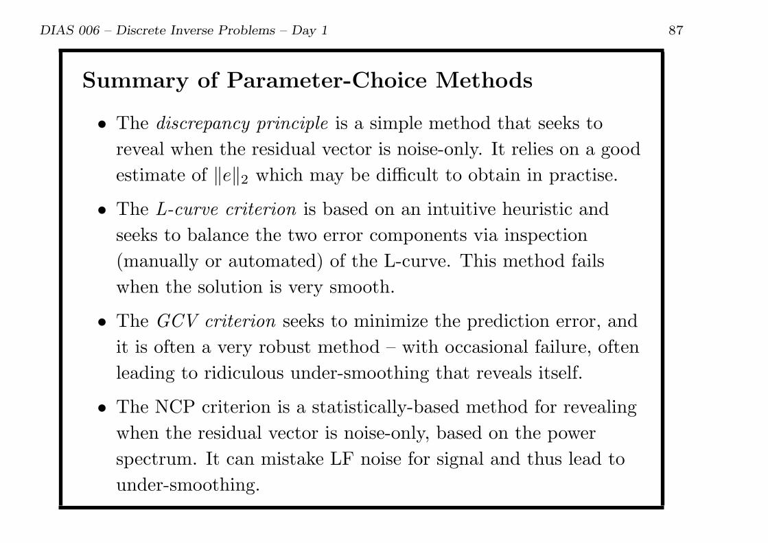
Summary of Parameter-Choice Methods

• The discrepancy principle is a simple method that seeks to

reveal when the residual vector is noise-only. It relies on a good

estimate of ∥e∥2 which may be difficult to obtain in practise.

• The L-curve criterion is based on an intuitive heuristic and

seeks to balance the two error components via inspection

(manually or automated) of the L-curve. This method fails

when the solution is very smooth.

• The GCV criterion seeks to minimize the prediction error, and

it is often a very robust method – with occasional failure, often

leading to ridiculous under-smoothing that reveals itself.

• The NCP criterion is a statistically-based method for revealing

when the residual vector is noise-only, based on the power

spectrum. It can mistake LF noise for signal and thus lead to

under-smoothing.

motivation: why inverse problems? - compute.dtu.dkpcha/airtoolsii/tutorial/dublinday1.pdf · 0 20...

Documents