motivation using feyncalc in your research … using feyncalc in your research summary and outlook...

MotivationUsing FeynCalc in your research

Summary and outlook

One-loop calculations with FeynCalc

Vladyslav Shtabovenko

in collaboration with R. Mertig and F. Orellana

Technische Universität München

IMPRS Young Scientist Workshop atRingberg Castle 2015

Physik-Department T30f

Physik-Department T30f (TUM) FeynCalc 1 / 27


Summary and outlook

Outline

1 MotivationQFT AutomationFeynCalc

2 Using FeynCalc in your research1-loop calculationsExample: Schwinger’s triumph

3 Summary and outlook



Summary and outlookQFT AutomationFeynCalc

WhatAutomation of QFT ≈ automatic symbolic or numeric evaluation ofFeynman diagramsThis talks: only symbolics

WhyFeynman diagrams → theoretical predictions for experimental observables:cross-sections, decay rates etc.Experiments are becoming more precise → theorists must reduce errors intheir predictions to keep up.Leading order (LO) in perturbation theory is mostly not enough, need togo at least to NLO or even higherNeed to evaluate hundreds, thousands or even millions of FeynmandiagramsImpossible to do by pen and paper!




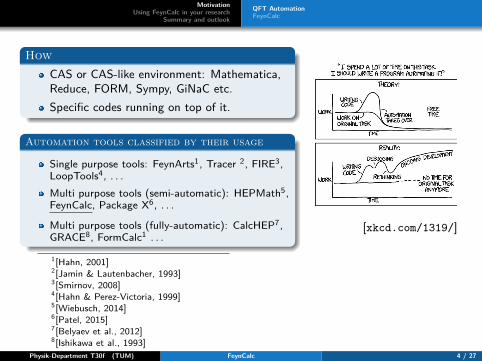
HowCAS or CAS-like environment: Mathematica,Reduce, FORM, Sympy, GiNaC etc.Specific codes running on top of it.

Automation tools classified by their usage

Single purpose tools: FeynArts1, Tracer 2, FIRE3,LoopTools4, . . .Multi purpose tools (semi-automatic): HEPMath5,FeynCalc, Package X6, . . .

Multi purpose tools (fully-automatic): CalcHEP7,GRACE8, FormCalc1 . . .

[xkcd.com/1319/]

1[Hahn, 2001]2[Jamin & Lautenbacher, 1993]3[Smirnov, 2008]4[Hahn & Perez-Victoria, 1999]5[Wiebusch, 2014]6[Patel, 2015]7[Belyaev et al., 2012]8[Ishikawa et al., 1993]


xkcd.com/1319/



FeynCalc is a Mathematica package for algebraic QFTcalculations

[Mertig et al., 1991]Suitable for evaluating both single expression and fullFeynman diagrams

Features

Extensive typesetting for better readability(using Mathematica’s TraditionalForm output)Tools for frequently occurring tasks like Lorentz index contraction, SU(N) algebra,Dirac matrix manipulation and traces, etc.(Contract, SUNSimplify, SUNTrace, DiracSimplify, DiracTrace,DiracEquation, DiracReduce, Schouten )Passarino-Veltman reduction of one-loop amplitudes to standard scalar integrals(OneLoop, OneLoopSimplify, TID, Tdec, PaVeReduce, ScalarProductCancel,FeynAmpDenominatorSimplify, FCLoop* )General tools for non-commutative algebra(DotSimplify, DotExpand, DeclareNonCommutative,UnDeclareNonCommutative, Commutator, Anticommutator)The calculation can be organized in many different ways (flexibility)




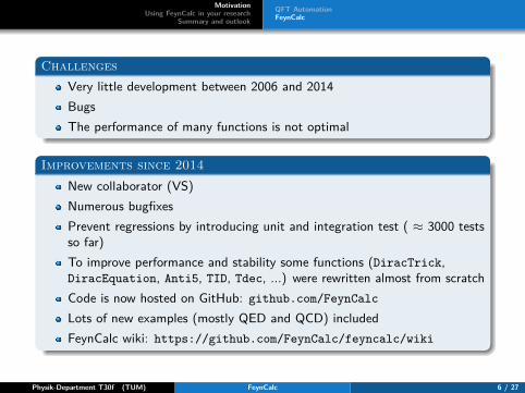
ChallengesVery little development between 2006 and 2014BugsThe performance of many functions is not optimal

Improvements since 2014New collaborator (VS)Numerous bugfixesPrevent regressions by introducing unit and integration test ( ≈ 3000 testsso far)To improve performance and stability some functions (DiracTrick,DiracEquation, Anti5, TID, Tdec, ...) were rewritten almost from scratchCode is now hosted on GitHub: github.com/FeynCalc

Lots of new examples (mostly QED and QCD) includedFeynCalc wiki: https://github.com/FeynCalc/feyncalc/wiki


github.com/FeynCalc

https://github.com/FeynCalc/feyncalc/wiki


Summary and outlook1-loop calculationsExample: Schwinger’s triumph

Ingredients of a 1-loop calculation in dimensional regularization (DR)∫d4 l

(2π)4(lµ lν)

l2 −m2 → µD−4∫

dDl(2π)D

(lµlν)l2 −m2

Simplification of the Dirac algebra (XFeynCalc)Reduction of tensor integrals to scalar integrals

Cancellation of scalar products and (XFeynCalc)Tensor decomposition (XFeynCalc)

Further simplification of scalar integralsPartial fractioning (XFeynCalc)IBP reduction (usually requires external tools )

Evaluation of master integrals (requires external tools)




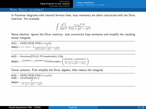
Why Dirac algebra?In Feynman diagrams with internal fermion lines, loop momenta are often contracted with the Diracmatrices. For example, ∫

dDl(2π)D

γνγµlν lµ

l2((l + p)2 −m2)

Naive solution: Ignore the Dirac matrices. Just uncontract loop momenta and simplify the resultingtensor integrals

In[1]:= GSD[l].GSD[l] FAD[l,{l+p,m}]Out[1]:= (γ · l).(γ · l)

1([l2]) ([(l + p)2 − m2])

In[2]:= Uncontract[%%,l]//FCLoopIsolate[#,{l}]&

Out[2]:= γ$AL$2494(1)

.γ$AL$2494(2)FCGV(LoopInt)

(l$AL$2494(1)l$AL$2494(2)

l2. ((l + p)2 − m2)

)Clever solution: First simplify the Dirac algebra, then reduce the integrals

In[3]:= GSD[l].GSD[l] FAD[l,{l+p,m}];In[4]:= DiracSimplify [%,l ]

Out[4]:=l2

l2. ((l + p)2 − m2)




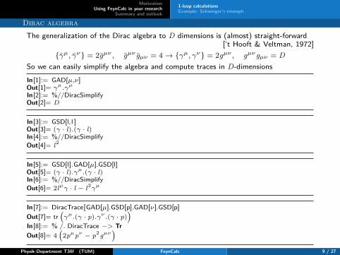
Dirac algebraThe generalization of the Dirac algebra to D dimensions is (almost) straight-forward

[’t Hooft & Veltman, 1972]{γµ, γν} = 2gµν , gµν gµν = 4→ {γµ, γν} = 2gµν , gµνgµν = D

So we can easily simplify the algebra and compute traces in D-dimensions

In[1]:= GAD[µ,ν]Out[1]= γ

µ.γ

µ

In[2]:= %//DiracSimplifyOut[2]= D

In[3]:= GSD[l,l ]Out[3]= (γ · l).(γ · l)In[4]:= %//DiracSimplifyOut[4]= l2

In[5]:= GSD[l].GAD[µ].GSD[l]Out[5]= (γ · l).γµ

.(γ · l)In[6]:= %//DiracSimplifyOut[6]= 2lµ

γ · l − l2γ

µ

In[7]:= DiracTrace[GAD[µ].GSD[p].GAD[ν].GSD[p]Out[7]= tr

(γ

µ.(γ · p).γν

.(γ · p))

In[8]:= % /. DiracTrace −> TrOut[8]= 4

(2pµpν − p2gµν

)Physik-Department T30f (TUM) FeynCalc 9 / 27



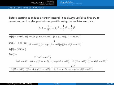
Cancelling scalar products

Before starting to reduce a tensor integral, it is always useful to first try tocancel as much scalar products as possible using the well-known trick

l · k = 12 (l + k)2 − 1

2 l2 − 12k2

In[1]:= SPD[l, p1] FVD[l, µ] FAD[{l, m0}, {l + p1, m1}, {l + p2, m2}]

Out[1]= lµ(l · p1)1

([l2 − m02]) ([(l + p1)2 − m12]) ([(l + p2)2 − m22])

In[2]:= SPC[#,l]

Out[2]=lµ(m02 − m12

)2 (l2 − m02) . ((l − p1)2 − m12) . ((l − p2)2 − m22)

−lµ

2 (l2 − m02) . ((l − p2)2 − m22)

−lµ

2 (l2 − m12) . ((l − p1 + p2)2 − m22)+

p1µ

2 (l2 − m12) . ((l − p1 + p2)2 − m22)




Passarino Veltman reduction

Passarino-Veltman reduction is the standard technique for the tensordecomposition of loop integrals.

[t’Hooft & Veltman, 1979][Passarino & Veltman, 1979]

Lorentz covariance allows us to rewrite any tensor integral as a linearcombination of all allowed Lorentz structuresThese structures are made of metric tensors and external momentaThey are also multiplied by scalar coefficients. These coefficients (akaPassarino-Veltman coefficient functions) can be computed either analyticallyor numerically.




∫dDl

(2π)Dlµlν

[l2 −m2][(l + p)2 −m2] = gµνB00 + pµpνB11

Contracting with gµν and pµpν we obtain a linear system of scalar equations∫dDl

(2π)Dl2

[l2 −m2][(l + p)2 −m2] = DB00 + p2B11∫dDl

(2π)D(l · p)2

[l2 −m2][(l + p)2 −m2] = p2B00 + p4B11

Solving this system we can determine the coefficients B00 and B11.




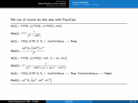
We can of course do this also with FeynCalc

In[1]:= FVD[l, µ] FVD[l, ν] FAD[{l, m0}]

Out[1]= lµlν 1[l2 − m02]

In[2]:= TID[1/(I Pi^2) %, l , UsePaVeBasis −> True]

Out[2]=m02A0

(m02)

gµν

D

In[3]:= FVD[l, µ] FAD[{l, m0}, {l + p1, m1}]

Out[3]:= lµ 1([l2 − m02]) ([(l + p1)2 − m12])

In[4]:= TID[1/(I Pi^2) %, l , UsePaVeBasis −> True, PaVeAutoReduce −> False]

Out[4]:= p1µB1(p12

,m02,m12

)




also for more complicated integrals

In[1]:= FVD[l, µ] FVD[l, ν] FVD[l , ρ] FAD[{l, m0}, {l + p1, m1}, {l + p2, m2}]

Out[1]= lµlν lρ 1([l2 − m02]) ([(l + p1)2 − m12]) ([(l + p2)2 − m22])

In[2]:= TID[1/(I Pi^2) %, l , UsePaVeBasis −> True, PaVeAutoReduce −> False]

Out[2]=(p1µgνρ + p1ν gµρ + p1ρgµν

)C001

(p12

,−2(p1 · p2) + p12 + p22, p22

,m02,m12

,m22)

+(p2µgνρ + p2ν gµρ + p2ρgµν

)C002

(p12

,−2(p1 · p2) + p12 + p22, p22

,m02,m12

,m22)

+p1µp1νp1ρC111(p12

,−2(p1 · p2) + p12 + p22, p22

,m02,m12

,m22)

+(p1νp1ρp2µ + p1µp1ρp2ν + p1µp1νp2ρ

)×C112

(p12

,−2(p1 · p2) + p12 + p22, p22

,m02,m12

,m22)

+(p1ρp2µp2ν + p1νp2µp2ρ + p1µp2νp2ρ

)×C122

(p12

,−2(p1 · p2) + p12 + p22, p22

,m02,m12

,m22)

+p2µp2νp2ρC222(p12

,−2(p1 · p2) + p12 + p22, p22

,m02,m12

,m22)




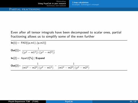
Partial fractioning

Even after all tensor integrals have been decomposed to scalar ones, partialfractioning allows us to simplify some of the even further

In[1]:= FAD[{p,m1},{p,m2}]

Out[1]=1

([p2 − m12]) ([p2 − m22])

In[2]:= Apart2[%]//Expand

Out[2]=1

(m12 − m22) (p2 − m12)−

1(m12 − m22) (p2 − m22)




As long as the kinematics inside the loop integral is general, we can write it interms of the 4 Passarino Veltman basis integrals A0, B0, C0 and D0.

In[1]:= ClearScalarProducts ;ScalarProduct[p1, p2] = 2 M^2;ScalarProduct[p1, p1] = M^2;ScalarProduct[p2, p2] = M^2;FVD[l, \[Mu]] FAD[{l, m0}, {l + p1, m1}, {l + p2, m2}];

Out[1]:= lµ 1([l2 − m02]) ([(l + p1)2 − m12]) ([(l + p2)2 − m22])

In[2]:= TID[%, l] // Isolate [#, FeynAmpDenominator] & //ReplaceAll[#, FeynAmpDenominator[x__] :>FRH[FeynAmpDenominator[x]]]&

Out[2]:=KK(147)

6M4 (l2 − m02) . ((l − p1)2 − m12) . ((l − p2)2 − m22)

+KK(141)

6M4 (l2 − m12) . ((l − p1)2 − m02)+

KK(143)6M4 (l2 − m02) . ((l − p1)2 − m12)

−KK(141)

6M4 (l2 − m22) . ((l − p2)2 − m02)−

KK(143)6M4 (l2 − m22) . ((l − p1 + p2)2 − m12)




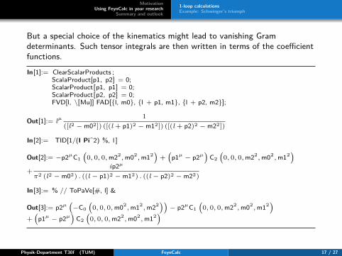
But a special choice of the kinematics might lead to vanishing Gramdeterminants. Such tensor integrals are then written in terms of the coefficientfunctions.

In[1]:= ClearScalarProducts ;ScalaProduct[p1, p2] = 0;ScalarProduct[p1, p1] = 0;ScalarProduct[p2, p2] = 0;FVD[l, \[Mu]] FAD[{l, m0}, {l + p1, m1}, {l + p2, m2}];

Out[1]:= lµ 1([l2 − m02]) ([(l + p1)2 − m12]) ([(l + p2)2 − m22])

In[2]:= TID[1/(I Pi^2) %, l ]

Out[2]:= −p2µC1(

0, 0, 0,m22,m02

,m12)

+(p1µ − p2µ

)C2(

0, 0, 0,m22,m02

,m12)

+ip2µ

π2 (l2 − m02) . ((l − p1)2 − m12) . ((l − p2)2 − m22)

In[3]:= % // ToPaVe[#, l] &

Out[3]:= p2µ(

−C0(

0, 0, 0,m02,m12

,m22))

− p2µC1(

0, 0, 0,m22,m02

,m12)

+(p1µ − p2µ

)C2(

0, 0, 0,m22,m02

,m12)




Feyncalc can algebraically simplify many standalone QFT expressions. Whatabout Feynman diagrams?

Generating Feynman diagramsFeynCalc itself can’t generate any diagrams⇒ Use FeynArtsSome objects in FeynCalc and FeynArts have same names (e.g.FourVector) which leads to issues⇒ Patch FeynArts to rename conflicting objectsThe output of FeynArts is incompatible with FeynArtsConvert it to FeynCalc via FCPrepareFAAmp




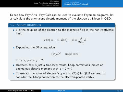
To see how FeynArts+FeynCalc can be used to evaluate Feynman diagrams, letus calculate the anomalous electric moment of the electron at 1-loop in QED.

g-2: Short reminderg is the coupling of the electron to the magnetic field in the non-relativisticlimit

V (x) = −~µ · ~B(x), ~µ = g2me

~S

Expanding the Dirac equation

(iγµDµ −me)ψ = 0

in 1/me yields g = 2.However, this is just a tree-level result. Loop corrections induce ananomalous electric moment with g − 2 6= 0To extract the value of electron’s g − 2 to O(α) in QED we need toconsider the 1-loop correction to the electron-photon vertex.




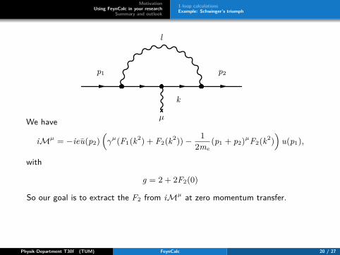
p1

l

p2

k

µWe have

iMµ = −ieu(p2)(γµ(F1(k2) + F2(k2))− 1

2me(p1 + p2)µF2(k2)

)u(p1),

with

g = 2 + 2F2(0)

So our goal is to extract the F2 from iMµ at zero momentum transfer.




We start with loading FeynCalc and FeynArts

In[1]:= $LoadFeynArts=True;<<FeynCalc‘$FAVerbose=0;

Then we use FeynArts to generate our diagram

In[2]:= topVertex = CreateTopologies[1, 1 −> 2, ExcludeTopologies −> {Tadpoles, WFCorrections}];

In[3]:= diagsVertex = InsertFields [topVertex, {F[2, {1}]} −> {V[1], F[2, {1}]}, InsertionLevel−> {Classes}, Model −> "SM", ExcludeParticles −> {S[1], S[2], S[3], V[3], V [2]}];

In[4]:= Paint[ diagsVertex , ColumnsXRows −> {2, 1}, Numbering −> None]




Next step is to convert the output of FeynArts into input for FeynCalc

In[5]:= ampVertex = Total@Map[ReplaceAll[#, FeynAmp[_, _, amp_, ___] :> amp] &,Apply[List , FCPrepareFAAmp[ CreateFeynAmp[diagsVertex, Truncated −> False,PreFactor −> −1], UndoChiralSplittings −> True]]] /.{InMom1 −> p1, OutMom2 −> p2, OutMom1 −> k, LoopMom1 −> q} /.k −> p1 − p2 /. q −> q + p1;Out[5]:=

−(

igLor2Lor3ε

∗Lor1(p1 − p2)(ϕ(p2,ME)

).(

iELγLor3).(γ ·(p2 + q

)+ ME

).(

iELγLor1).(

γ ·(p1 + q

)+ ME

).(

iELγLor2).(ϕ(p1,ME)

))/(

(p1 + q)2 − ME2).(

(p2 + q)2 − ME2).q2

after which we set up the kinematics, convert the obtained amplitude into aD-dimensional one and chop off the polarization vector

In[6]:= ClearScalarProducts ;In[7]:= ScalarProduct[p1, p1] = ME^2;In[8]:= ScalarProduct[p2, p2] = ME^2;In[9]:= ScalarProduct[k, k] = 0;In[10]:= ScalarProduct[p1, p2] = ME^2;In[11]:= ampVertex1 = (ampVertex // ChangeDimension[#, D] &)//ReplaceAll[#, Pair [Momentum[Polarization[___], ___], ___] :> 1] &;




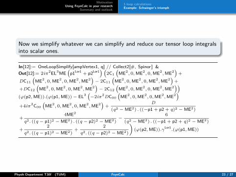
Now we simplify whatever we can simplify and reduce our tensor loop integralsinto scalar ones.

In[12]:= OneLoopSimplify[ampVertex1, q] // Collect2[#, Spinor ] &Out[12]:= 2iπ2EL3ME

(p1Lor1 + p2Lor1

)(2C1(ME2

, 0,ME2, 0,ME2

,ME2)

+DC11

(ME2

, 0,ME2, 0,ME2

,ME2)

− 2C11(ME2

, 0,ME2, 0,ME2

,ME2)

++DC12

(ME2

, 0,ME2, 0,ME2

,ME2)

− 2C12(ME2

, 0,ME2, 0,ME2

,ME2))

(ϕ(p2,ME)).(ϕ(p1,ME)) − EL3(

−2iπ2DC00(ME2

, 0,ME2, 0,ME2

,ME2)

+4iπ2C00(ME2

, 0,ME2, 0,ME2

,ME2)

+D

(q2 − ME2) . ((−p1 + p2 + q)2 − ME2)

+4ME2

q2. ((q − p1)2 − ME2) . ((q − p2)2 − ME2)−

6(q2 − ME2) . ((−p1 + p2 + q)2 − ME2)

+2

q2. ((q − p1)2 − ME2)+

2q2. ((q − p2)2 − ME2)

)(ϕ(p2,ME)).γLor1.(ϕ(p1,ME))




Remember that to extract F2(0) we need to look only at the piece proportional to(p1 + p2)µ. So let us drop the γµ-piece

In[13]:= ampVertex3 = ampVertex2 // ReplaceAll[#,FCI[GAD[Lor1]] :> 0] & // DotSimplifyOut[13]:= 2iπ2EL3ME

(p1Lor1 + p2Lor1

)(2C1(ME2

, 0,ME2, 0,ME2

,ME2)

+DC11

(ME2

, 0,ME2, 0,ME2

,ME2)

− 2C11(ME2

, 0,ME2, 0,ME2

,ME2)

++DC12

(ME2

, 0,ME2, 0,ME2

,ME2)

− 2C12(ME2

, 0,ME2, 0,ME2

,ME2))

(ϕ(p2,ME)).(ϕ(p1,ME))

The Passarino-Veltman coefficient functions C1,C11 and C12 that appear in theresult can be analytically evaluated using other packages (e.g. Package X). Here wejust substitute their values

In[14]:= ampVertex4 = ampVertex3 /. {PaVe[1, {ME^2, 0, ME^2}, {0, ME^2, ME^2}, OptionsPattern[]] −> 1/(32 Pi^4 ME^2),PaVe[1, 1, {ME^2, 0, ME^2}, {0, ME^2, ME^2}, OptionsPattern[]] −> −(1/(96 Pi^4 ME^2)),PaVe[1, 2, {ME^2, 0, ME^2}, {0, ME^2, ME^2}, OptionsPattern[]] −> −(1/(192 Pi^4 ME^2))}

Out[14]:= 2iπ2EL3ME(

332π4ME2 −

D64π4ME2

)(p1Lor1 + p2Lor1

)(ϕ(p2,ME)).(ϕ(p1,ME))

As expected, F2(0) is free of any divergences. So we can safely do the limit D → 4




In[15]:= ampVertex5 = ampVertex4 // ChangeDimension[#, 4] & // ReplaceAll[#, D −> 4] &

Out[15]:=iEL3

(p1Lor1 + p2Lor1

)(ϕ(ME, p2)

).(ϕ(ME, p1

))

16π2ME

What we obtained so far is nothing else than ie2me

(p1 + p2)µF2(0)u(p2)u(p1).

Dividing by the numerical prefactor and substituting e2 = 4π2α yields

In[16]:= (ampVertex5/((I EL)/(2 ME))) // ReplaceAll [#, {EL^2 −> AlphaFS 4 \[Pi], Spinor[__].Spinor[__] :> 1, FCI[FV[p1, _] + FV[p2, _]] :> 1}] &

Out[16]:=α

2π

In[17]:= N[1/137 1/(2 Pi)]Out[17]:= 0.00116171

so that

F2(0) = α

2πand

g − 22 = α

2π +O(α2)

which was one of the greatest triumphs of QED in the last century[Schwinger, 1948]



Summary and outlook

What I learned while developing FeynCalc

General recommendationsUse a version control system (e.g. git, mercurial)Use a testing framework to prevent regressions (e.g. MUnit forMathematica, pyunit for Python, CppUnit for C++)

Mathematica specific recommendationsHave a look at Wolfram WorkbenchRead at least one book about Mathematica programming



Summary and outlook

SummaryFeynCalc is a Mathematica package for algebraic calculations in QFT andsemi-automatic evaluation of Feynman diagramsAfter a long period of low-activity the active development has beenrestarted 2014The upcoming FeynCalc 9.0 will include numerous bug fixes but alsoperformance enhancements and new features

TODOs:More regression and integration tests (goal: full code coverage)More worked out examplesFinish the manualStable interfaces to other useful software tools for symbolic/numericevaluation


Backup

Issues with γ5

There is no unique way to handle γ5 = iγ0γ1γ2γ3 in DRIn D-dimensions, the relations

{γ5, γµ} = 0

and

tr(γ5γµγνγργσ) 6= 0

cannot be simultaneously satisfied.In other words, there is a conflict between the anticommutativity of γ5 andthe cyclicity property of Dirac traces that involve and odd number of γ5

[Chanowitz et al., 1979][Jegerlehner, 2001]


Backup

Issues with γ5

We can stick to the anticommuting γ5 in D-dimensions. This is fine, aslong as we have only traces with an even number of γ5.⇒ Naive dimensional regularization (NDR)To compute traces with an odd number of γ5 unambiguously, we need anadditional prescription⇒ Kreimer’s prescription

[Kreimer, 1990]⇒ Larin-Gorishny-Akyeampong-Delburgo prescription

[Larin, 1993]Or we can accept that γ5 is a purely 4-dimensional object and thereforedoesn’t anitcommute with D-dimensional Dirac matrices

[’t Hooft & Veltman, 1972][Breitenlohner & Maison, 1977]

⇒ Breitenlohner-Maison- t’Hooft Veltman scheme (BMHV)


Backup

By default, FeynCalc works with an anticommuting γ5

In[1]:= GAD[µ,ν,ρ].GA[5].GAD[σ,τ ,κ].GA[5]Out[1]= γ

µ.γ

ν.γ

ρ.γ

5.γ

σ.γ

τ.γ

κ.γ

5

In[2]:= %//DiracSimplifyOut[2]= −γµ

.γν.γ

ρ.γ

σ.γ

τ.γ

κ

Trying to compute a chiral trace in the naive scheme produces an error message:In[1]:= DiracTrace[GAD[µ,ν,ρ,σ,τ ,κ].GA[5]]Out[1]= tr

(γ

µ.γ

ν.γ

ρ.γ

σ.γ

τ.γ

κ.γ

5)

In[2]:= % /. DiracTrace −> Tr


Backup

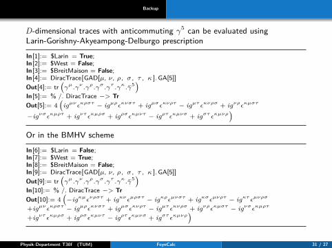
D-dimensional traces with anticommuting γ5 can be evaluated usingLarin-Gorishny-Akyeampong-Delburgo prescription

In[1]:= $Larin = True;In[2]:= $West = False;In[3]:= $BreitMaison = False;In[4]:= DiracTrace[GAD[µ, ν, ρ , σ , τ , κ ]. GA[5]]Out[4]:= tr

(γ

µ.γ

ν.γ

ρ.γ

σ.γ

τ.γ

κ.γ

5)

In[5]:= % /. DiracTrace −> TrOut[5]:= 4

(igµν

εκρστ − igµρ

εκνστ + igµσ

εκνρτ − igµτ

εκνρσ + igνρ

εκµστ

−igνσε

κµρτ + igντε

κµρσ + igρσε

κµντ − igρτε

κµνσ + igστε

κµνρ)

Or in the BMHV scheme

In[6]:= $Larin = False;In[7]:= $West = True;In[8]:= $BreitMaison = False;In[9]:= DiracTrace[GAD[µ, ν, ρ , σ , τ , κ ]. GA[5]]Out[9]:= tr

(γ

µ.γ

ν.γ

ρ.γ

σ.γ

τ.γ

κ.γ

5)

In[10]:= % /. DiracTrace −> TrOut[10]:= 4

(−igκµ

ενρστ + igκν

εµρστ − igκρ

εµνστ + igκσ

εµνρτ − igκτ

εµνρσ

+igµνε

κρστ − igµρε

κνστ + igµσε

κνρτ − igµτε

κνρσ + igνρε

κµστ − igνσε

κµρτ

+igντε

κµρσ + igρσε

κµντ − igρτε

κµνσ + igστε

κµνρ)


Backup

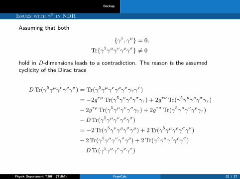
Issues with γ5 in NDR

Assuming that both

{γ5, γµ} = 0,Tr{γ5γµγνγργσ} 6= 0

hold in D-dimensions leads to a contradiction. The reason is the assumedcyclicity of the Dirac trace

D Tr(γ5γµγνγργσ) = Tr(γ5γµγνγργσγτγτ )

= −2gτµ Tr(γ5γνγργσγτ ) + 2gτν Tr(γ5γµγργσγτ )− 2gτρ Tr(γ5γµγνγσγτ ) + 2gτσ Tr(γ5γµγνγργτ )−D Tr(γ5γµγνγργσ)= −2 Tr(γ5γνγργσγµ) + 2 Tr(γ5γµγργσγν)− 2 Tr(γ5γµγνγσγρ) + 2 Tr(γ5γµγνγργσ)−D Tr(γ5γµγνγργσ)


Backup

Issues with γ5 in NDR

Using that Tr(γ5γµγν) = 0 we have

D Tr(γ5γµγνγργσ) = (8−D) Tr(γ5γµγνγργσ)

or

(4−D) Tr(γ5γµγνγργσ) = 0.

This implies that Tr(γ5γµγνγργσ) is zero for all D 6= 4.But if we demand the trace to be meromorphic in D, then the above traceshould be zero also for D = 4,Hence, we cannot recover the 4-dimensional Dirac algebra at D = 4.


Backup

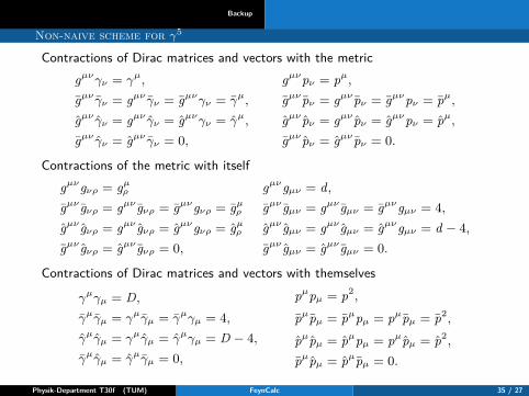
Non-naive scheme for γ5

In the Breitenlohner-Maison-’t Hooft-Veltman scheme we are dealing withmatrices in D, 4 and D-4 dimensions. Many identities of the BMHV algebra canbe proven by by decomposing Dirac matrices into two pieces

dim(γµ) = d,dim(γµ) = 4,dim(γµ) = d − 4.

γµ = γµ + γµ,

gµν = gµν + gµν ,pµ = pµ + pµ.

(Anti)commuatators between γ’s in different dimensions

{γµ, γν} = 2gµν ,{γµ, γν} = {γµ, γν} = 2gµν ,{γµ, γν} = {γµ, γν} = 2gµν ,{γµ, γν} = 0{γµ, γ5} = [γµ, γ5] = 0,{γµ, γ5} = {γµ, γ5} = 2γµγ5 = 2γ5γµ.


Backup

Non-naive scheme for γ5

Contractions of Dirac matrices and vectors with the metricgµνγν = γµ,

gµν γν = gµν γν = gµνγν = γµ,

gµν γν = gµν γν = gµνγν = γµ,

gµν γν = gµν γν = 0,

gµνpν = pµ,gµν pν = gµν pν = gµνpν = pµ,gµν pν = gµν pν = gµνpν = pµ,gµν pν = gµν pν = 0.

Contractions of the metric with itselfgµνgνρ = gµρgµν gνρ = gµν gνρ = gµνgνρ = gµρgµν gνρ = gµν gνρ = gµνgνρ = gµρgµν gνρ = gµν gνρ = 0,

gµνgµν = d,gµν gµν = gµν gµν = gµνgµν = 4,gµν gµν = gµν gµν = gµνgµν = d − 4,gµν gµν = gµν gµν = 0.

Contractions of Dirac matrices and vectors with themselves

γµγµ = D,γµγµ = γµγµ = γµγµ = 4,γµγµ = γµγµ = γµγµ = D − 4,γµγµ = γµγµ = 0,

pµpµ = p2,

pµpµ = pµpµ = pµpµ = p2,

pµpµ = pµpµ = pµpµ = p2,

pµpµ = pµpµ = 0.


Backup

Larin’s scheme

Larin-Gorishny-Akyeampong-Delburgo prescription allows one to useanticommuting γ5 in D-dimensions but compute the chiral traces, such, that theresult is expected to be equivalent with the BMHV scheme, if we have only oneaxial-vector current. The prescription is essentially

Anticommute γ5 to the right inside the trace

Replace γµγ5 with − i6ε

µαβσγαγβγσ

Treat εµαβσ as if it were D-dimensional, i.e.εµαβσεµαβσ = −D(D3 − 6D2 + 11D − 6) instead of −24.


Backup

Schouten’s identity

In an n-dimensional space, a totally antisymmetric tensor with n + 1 indicesvanishes. For example, eijkl = 0 if i,j,k and l are Cartesian indices that run from1 to 3, because no matter how you choose the values of the indices, you willalways have at least two indices with the same value.

4D space

εµνρσpτ + ενρστpµ + ερστµpν + εστµνpρ + ετµνρpσ = 0

εµνρσgτκ + ενρστgµκ + ερστµgνκ + εστµνgρκ + ετµνρgσκ = 0

3D space

εijkpl − εjklpi + εkljpj − εlijpk = 0

εijkglm − εjklpim + εkljgjm − εlijgkm = 0


Backup

Definitions of the PaVe scalar integrals (LoopTools convention)

A0(m0) = µ4−D(4π)4−D

2

∫dDqiπ D

2

1q2 −m2

0

B0(p1,m0,m1) = µ4−D(4π)4−D

2

∫dDqiπ D

2

1(q2 −m2

0)((q + p1)2 −m21)

C0(p1, p2,m0,m1,m2)

= µ4−D(4π)4−D

2

∫dDqiπ D

2

1(q2 −m2

0)((q + p1)2 −m21)((q + p1 + p2)2 −m2

2)

D0(p1, p2, p3,m0,m1,m2,m3)

= µ4−D(4π)4−D

2

∫dDqiπ D

2

1(q2 −m2

0)((q + p1)2 −m21)((q + p1 + p2)2 −m2

2)

× 1((q + p1 + p2 + p3)2 −m2

3)


Backup

Normalization of the PaVe scalar integrals

Passarino-Veltman scalar functions are normally related to the text bookintegrals by a factor of (16π2)/i, e.g.

µ4−D∫

dDq(2π)D

1q2 −m2

0= i

16π2 A0(m0)

To see this observe that1

(2π)D = 116π2

12D−4πD−2 = 1

16π24

4−D2

πD−2 = 116π2

(4π)4−D

2

πD2

However, in FeynCalc the PaVe functions are normalized as

µ4−D 1iπ2

∫dDq(. . .). Hence, we have

A0,FC (m0) = (2π)D−4A0(m0) = (2π)D

iπ2 µ4−D∫

dDq(2π)D

1q2 −m2

0

On the other hand, if the prefactor 1(2π)D is implicit (i.e. it is understood but

not written down explicitly) in the calculation, then it is enough to perform thereplacement

A0,FC (m0)→ 1iπ2 µ

4−D∫

dDq(2π)D

1q2 −m2

0Physik-Department T30f (TUM) FeynCalc 39 / 27

Backup

Belyaev, A., Christensen, N. D., & Pukhov, A. (2012).CalcHEP 3.4 for collider physics within and beyond the Standard Model.

Breitenlohner, P. & Maison, D. (1977).Dimensional renormalization and the action principle.Communications in Mathematical Physics, 52, 11–38.

Chanowitz, M., Furman, M., & Hinchliffe, I. (1979).The axial current in dimensional regularization.Nuclear Physics B, 159(1-2), 225–243.

Hahn, T. (2001).Generating Feynman Diagrams and Amplitudes with FeynArts 3.Comput.Phys.Commun., 140, 418–431.

Hahn, T. & Perez-Victoria, M. (Comput.Phys.Commun.118:153-165,1999).Automatized One-Loop Calculations in 4 and D dimensions.Comput.Phys.Commun., 118:153-165,1999.

Ishikawa, T. et al. (1993).GRACE manual: Automatic generation of tree amplitudes in StandardModels: Version 1.0.Jamin, M. & Lautenbacher, M. E. (1993).


Backup

TRACER version 1.1.Computer Physics Communications, 74(2), 265–288.

Jegerlehner, F. (Eur.Phys.J.C18:673-679,2001).Facts of life with gamma(5).Eur.Phys.J.C, 18:673-679,2001.

Kreimer, D. (1990).The γ5-problem and anomalies — A Clifford algebra approach.Phys. Lett. B, 237(1), 59–62.

Larin, S. A. (1993).The renormalization of the axial anomaly in dimensional regularization.Phys. Lett. B, 303, 113–118.

Mertig, R., Böhm, M., & Denner, A. (1991).Feyn Calc - Computer-algebraic calculation of Feynman amplitudes.Computer Physics Communications, 64(3), 345–359.

Passarino, G. & Veltman, M. (1979).One Loop Corrections for e+ e- Annihilation Into mu+ mu- in theWeinberg Model.Nucl.Phys., B160, 151.


Backup

Patel, H. H. (2015).Package-X: A Mathematica package for the analytic calculation of one-loopintegrals.

Schwinger, J. (1948).On Quantum-Electrodynamics and the Magnetic Moment of the Electron.Phys. Rev., 73(4), 416–417.

Smirnov, A. V. (2008).Algorithm FIRE – Feynman Integral REduction.JHEP, 0810:107,2008.

t’Hooft, G. & Veltman, M. (1979).Scalar one-loop integrals.Nuclear Physics B, 153, 365–401.

Wiebusch, M. (2014).HEPMath: A Mathematica Package for Semi-Automatic Computations inHigh Energy Physics.

’t Hooft, G. & Veltman, M. (1972).Regularization and renormalization of gauge fields.Nuclear Physics B, 44(1), 189–213.


motivation using feyncalc in your research … using feyncalc in your research summary and outlook...

Documents