HAL Id: hal-01489043https://hal.archives-ouvertes.fr/hal-01489043

Submitted on 16 Mar 2017

HAL is a multi-disciplinary open accessarchive for the deposit and dissemination of sci-entific research documents, whether they are pub-lished or not. The documents may come fromteaching and research institutions in France orabroad, or from public or private research centers.

L’archive ouverte pluridisciplinaire HAL, estdestinée au dépôt et à la diffusion de documentsscientifiques de niveau recherche, publiés ou non,émanant des établissements d’enseignement et derecherche français ou étrangers, des laboratoirespublics ou privés.

Motion Discontinuity-Robust Controller for SteerableMobile Robots

Mohamed Sorour, Andrea Cherubini, Philippe Fraisse, Robin Passama

To cite this version:Mohamed Sorour, Andrea Cherubini, Philippe Fraisse, Robin Passama. Motion Discontinuity-RobustController for Steerable Mobile Robots. IEEE Robotics and Automation Letters, IEEE 2017, 2 (2),pp.452-459. �10.1109/LRA.2016.2638466�. �hal-01489043�

Motion Discontinuity-Robust Controller for Steerable Mobile Robots

Mohamed Sorour1,2, Andrea Cherubini1, Philippe Fraisse1, and Robin Passama1

Abstract— Steerable wheeled mobile robots (SWMR) areable to perform arbitrary 3D planar trajectories, only afterinitializing the steer joint vector to the proper values. Theserobots employ fully steerable conventional wheels. Hence, theyhave higher load carrying capacity than their holonomic coun-terparts, and as such are preferable for industrial applications.Industrial setups nowadays are being prepared for the emergingfield of human-robot collaboration/cooperation. Such field ishighly dynamic, due to fast moving human workers, sharingthe operation space. This imposes the need for human safe tra-jectory generators, that can lead to frequent halts in motion, re-planning, and to sudden, discontinuous changes in the positionof the robot’s instantaneous center of rotation (ICR). Indeed,this requires steer joint reconfiguration to the newly computedtrajectory. This issue is almost ignored in the literature, andmotivates this work. The authors propose a new ICR-basedkinematic controller, that is capable of handling discontinuityin commanded velocity, while respecting the maximum jointperformance limit. This is done by formulating a quadraticoptimization problem with linear constraints in the 2D ICRspace. The controller is also robust against representation andkinematic singularities. It has been tested successfully on theNeobotix-MPO700 industrial mobile robot.

Index Terms— Steerable Wheeled Mobile Robots, Pseudo-omni Mobile Robots, Nonholonomic Omnidirectional WheeledMobile Robots, Kinematic Control.

I. INTRODUCTION

Steerable wheeled mobile robots gain mobility by employ-ing fully steerable wheels, having two active joints, one forsteering, and another for driving. Despite having only one de-gree of mobility (DOM) (defined here as the instantaneouslyaccessible degrees of freedom DOF), corresponding to therotation about the instantaneous center of rotation (ICR),such robots can perform complex 3D planar trajectories. Thiscan be done only after orienting the wheels to the properangles, depending on the trajectory to be performed. Fullyomnidirectional robots, on the other hand, employing eithercastor, Swedish or omni wheels, have 3DOM and, as such,can instantaneously track any desired trajectory. However,this type of wheels has limited load carrying capacity, andmay cause vibration during robot motion. For these reasons,SWMR are the preferred choice for industrial setups.

Due to their wide use in the industry, many researchefforts have been made to enhance their performance, againstkinematic (ICR at the steering joint axis) and representation(from the mathematical model) singularities. The latter havebeen solved, in the case of SWMR with three or more wheels,by using the 3D Cartesian velocity in deriving the kinematicmodel [1]. The former was addressed as a constraint to robotmotion in [2], or by using repulsive potential fields in [3],[4], [5]. However, reduction in robot maneuverability, by

1Interactive Digital Human group IDH, Laboratory for Computer Sci-ence , Micro-electronics and Robotics LIRMM, University of Mont-pellier CNRS, 860 rue Saint Priest, 34090 Montpellier, France.firstname.lastname@lirmm.fr

2PSA Peugeot-Citroen, Velizy Villacoublay, France.

employing these methods, is not acceptable, and attemptswere made to deal with kinematic singularity by handlingthe maximum joint limits [6] and by changing coordinatesystem [7]. Steering mechanical limits were also studied in[5] and [8]. Simulations in [7] do not indicate the behaviorof the steer joints in terms of respecting the velocity limits atkinematic singularity, while in [6], it is shown that the steerrate will saturate and keep operating at the maximum limit.

On the other hand, to the best of the authors knowledge,no thorough investigation has been conducted on the issueof reorienting the wheels, once discontinuity in the robottrajectory occurs. Usually, steer reconfiguration is performedin a manual fashion, depending on the test trajectory. Thisis found in the literature under various designations, e.g.”initial phase” in [1], and ”open-loop starting procedure”in [2]. Although an ICR-based controller is the most suitedto handle such cases, the work in [6] and [9] is limited by theassumption of continuous and differentiable desired signal,whereas in [5] the singularities imposed by the ICR-basedmodel are handled by reducing the robot maneuverability.

Such situation - discontinuity in robot motion - is morelikely to happen nowadays, in the emerging field of human-robot collaboration. Mobile robots working in the vicinityof fast moving human workers, will usually encounter dis-continuity in the online computed trajectory. In case of staticobstacles, the online planner can be less restricted in the formof the output trajectory, so that smooth behavior can alwaysbe expected. Instead, here, sudden appearance of an activeworker can result in prohibiting motion, and re-routing tofollow other trajectories. In such cases, the state of the artwill fail to provide proper solutions.

In this work, we propose a kinematic control frameworkthat is:

1) robust against trajectory discontinuity,2) capable of handling kinematic singularity,3) compliant with the maximum steer joint limits in terms

of velocity and acceleration (or jerk, seamlessly).The framework consists of two decoupled kinematic con-trollers: a Cartesian-velocity based controller, and an ICR-based one. The former is used to control the drive rate ”wheelspeed”, employing a Cartesian space kinematic model. Thelatter controls the steering rate, while respecting the maxi-mum steer joint limits, by using optimization to locate the”next sample time” ICR coordinates. The developed 3DCartesian space kinematic model is free from representa-tional singularity, while the kinematic singularities are beinghandled in the 2D ICR space controller. The benefit of usingseparate kinematic controllers for the drive and steering rates,is does not require mapping the 2D ICR-coordinate space tothe 3D Cartesian space, hence avoids associated singularitiesand inconveniences. Thanks to the formulated optimizationproblem, discontinuity in robot velocity trajectory is handled,while respecting the steer joint limits.

In the following, section II presents the Cartesian spacekinematic model. The velocity discontinuity robust controlleris detailed in section III. Experiments are depicted in sectionIV. Conclusions are finally given in section V.

II. KINEMATIC MODEL

The kinematic model presented in this section (detailed inprevious work by the authors [10]) is inspired by the pioneerwork of Muir [11], Campion [12], Betourne [13] and Low etal. [14]. The schematic of a SWMR is shown in Fig. 1 for a4 wheeled robot. However, the model is generic for SWMRwith number of wheels N ≥ 3.

A. Cartesian Space 3D Model Formulation

Let FI = (oI ,xI ,yI , zI) be the inertial frame, Fb =(ob,xb,yb, zb) the mobile base frame, with origin ob locatedat the base geometric center, Fhi = (ohi,xhi,yhi, zhi) theith hip frame (i = 1, . . . , N ), attached to the fixed part of thesteering joint, and related to the base frame by a fixed trans-formation matrix, and Fsi = (osi,xsi,ysi, zsi) the steeringframe, attached to the movable part. The hip and steeringframes share the same origin, with relative orientation βi(the steering angle). Frame Fwi = (owi,xwi,ywi, zwi) isattached to (but not rotating with) the ith wheel, assignedsuch that xwi points along the heading of the wheel, whichrotates about ywi by the driving angle φi. All the frameshave the z axis pointing upwards. Let the mobile base posew.r.t. the inertial frame define the 3D task space coordinatesξ =

[x y θ

]T. A left superscript is added to indicate

the frame in which the pose is expressed, for instance Iξand bξ denote the robot pose, expressed in the inertial andbase frames respectively. In the sequel, the left superscriptis omitted in case of vectors expressed in the base frame tolighten the notation, unless otherwise specified.

Considering the ith wheel velocity vci =[vti vni 0

]Tat the ground contact point oci (expressed in the wheel frameFwi), with vti and vni respectively the ith tangential andnormal velocities, it can be shown that [10]:

vti = f(βi)bξ + dβi − rwφi, (1)

vni = g(βi)bξ, (2)

f(βi) =[c(βi) s(βi) d− hyic(βi) + hxis(βi)

],

g(βi) =[−s(βi) c(βi) hxic(βi) + hyis(βi)

],

where hxi = ±b and hyi = ±a denote the position of the ithhip frame origin ohi in the base frame, c(∗) and s(∗) shorthand cos(∗) and sin(∗) respectively. The parameters d and rware the steerable wheel offset and radius respectively. Settingvti = 0 and vni = 0, (1) and (2) represent the rolling withno slipping and the no lateral skidding kinematic constraints,respectively. The no skidding constraint imposes restrictionson the robot motion (the wheel cannot move sideways), andforces the existence of a unique ICR point, around which thebase frame and all wheels must rotate. From such constraint,we construct the kinematic constraint matrix G(β) as:

G(β)N×3 =[g(β1)T ... g(βN )T

]T. (3)

𝒙𝑏

𝒚𝑏

𝑜𝑏

𝒙𝑤2

𝑜𝑤1

𝑜ℎ1, 𝑜𝑠1

2𝑏

𝑜𝑤𝑖

𝑜𝑐𝑖

𝒙𝑤𝑖 𝒚𝑤𝑖

𝒗𝑡𝑖

𝒗𝑛𝑖

𝒛𝑤𝑖

𝒙𝑤3

𝒙𝑤4

𝒙𝐼

𝒚𝐼

𝑜𝐼

𝜑1

𝛽1

𝒙ℎ1

𝒚ℎ1

𝒙𝑠1 𝒚𝑠1

𝒙𝑤1 𝒚𝑤1 𝑑

𝑟𝑤

2𝑎

Fig. 1: Schematic model of a four wheeled SWMR.

Equation (2) is differentiated w.r.t time, rearranged to eval-uate the required steer joint rate when vni = 0 as:

βi =−g(βi)ξdg(βi)d(βi)

ξ. (4)

Then, the wheel drive rate is obtained from (1), when vti =0:

φi =1

rwf(βi)ξ +

d

rwβi. (5)

Equations (4) and (5) represent the SWMR inverse actuationkinematic model (IAKM).

B. Odometry Model

In order to compute the task space velocity response fromthe joint space velocity measurements, we need the odometrymodel, or the forward actuation kinematic model (FAKM):

ξ = F+(d)(β)(rw

ˆφ− dˆβ), (6)

F (β)N×3 =[f(β1)T ... f(βN )T

]T,

where the hat symbol ˆ indicates a measurement value andF+(d)(∗) denotes the damped pseudo-inverse of F (∗), evalu-

ated using [15] and [16]:

F+(d)(∗) = (F T (∗)F (∗) + δ2I3×3)−1F T (∗),

with δ ∈ R the damping factor. We use the dampedpseudo-inverse to overcome algorithmic singularities, occur-ring when the mobile base moves with null angular velocity(all steer angles identical), as in such case, F (β) loses rank.

𝑰𝑪𝑹∗

𝑰𝑪𝑹 ∗

𝝃 ∗

Mapping the 3D Cartesian Space

Commands to the 2D ICR Space

ICR-Point Velocity

Controller

INVERSE ACTUATION

MODEL

STEERABLE WHEELED

MOBILE ROBOT

HIGH LEVEL

PERCEPTION/ TASK CONTROLLER

Steer Configuration to ICR Point Coordinates

𝑰𝑪𝑹𝑐𝑢𝑟𝑟

𝝃 𝑟𝑒𝑓

𝝃 𝐼 𝝃

𝑏

FORWARD ACTUATION

MODEL 𝑰 − 𝑮𝑟𝑒𝑓(𝑑)

+ 𝑮𝑟𝑒𝑓

𝜷 𝑟𝑒𝑓 𝜷𝑟𝑒𝑓

𝝃 ∗

QP Optimization to Obtain a

Feasible 𝑰𝑪𝑹𝑛𝑒𝑥𝑡

Respecting the Joint Limits

ICR Point to Steer Joint Coordinates

𝑰𝑪𝑹𝑛𝑒𝑥𝑡

𝝋 𝑟𝑒𝑓

3D Cartesian Space Velocity

Controller

𝝃 𝑟𝑒𝑓(𝑖𝑛𝑖𝑡) 𝑹

𝐼𝑏

𝜷

𝜷 𝜷 , 𝝋

Kinematic Singularity Treatment 𝑰𝑪𝑹𝑟𝑒𝑓

Fixing Numeric Issues

Section III.A

Section III.B

Section III.C

Section III.D

Section III.E

𝜷𝑛𝑒𝑥𝑡

Fig. 2: Proposed control framework.

III. DISCONTINUITY ROBUST ICR-POINT CONTROLLER

In this section, we present our control framework forinjecting the steer joint initialization in the trajectory per-formed by SWMR, and for handling run-time trajectorydiscontinuities, which ”depending on the application” can beoften necessary, especially in human robot interaction tasks.

The whole framework is depicted in Fig. 2. The desired3D Cartesian space robot motion (ξ∗, and ξ∗) is generatedby a high level perception controller (out of the scope ofthis work). This is then mapped to the 2D ICR space, andthe output desired ICR motion (ICR∗, and ˙ICR

∗) is fed

to the ICR velocity controller, along with the current ICRcoordinates ICRcurr. The output reference signal ICRref

is then used by an optimization algorithm to decide the”next sample time” ICR coordinates ICRnext that willminimize the quadratic cost error: ‖ICRref − ICRnext‖22while respecting the joint performance limits formulated aslinear constraints. We use the ICRref rather than ICR∗ inthe cost function in order to obtain smooth behavior since itis error dependant. The corresponding steer joint referencesignal βref is then evaluated (while fixing the numeric issuesinvolved) and differentiated, to obtain the βref that is sent tothe robot low level controller. At the same time, a decoupledrobot twist controller is implemented, the initial output ofwhich ξref(init) is projected onto the null space of the”next sample time” robot configuration (represented by thekinematic constraint matrix G(βref )), to obtain the feasiblecontrol signal ξref . The reference wheel rate φref is thenobtained using the IAKM in (5). The colored blocks in Fig.(2) are detailed in each of the following subsections.

A. ICR Velocity ControllerIn Fig. 2, the desired base frame motion is the output

of the high level perception block. As shown in Fig. 3, thecorresponding desired ICR coordinates, expressed in baseframe, ICR∗ =

[X∗ Y ∗

]T, are usually evaluated using:

X∗ = −y∗/θ∗, Y ∗ = x∗/θ∗.

However, this formula is singular in pure translation motion.Alternatively, here we propose to use:

X∗ = R∞ tanh

(( −y∗

θ∗ + sign(θ∗)δ1

)/R∞

),

Y ∗ = R∞ tanh

(( x∗

θ∗ + sign(θ∗)δ1

)/R∞

),

(7)

sign(θ∗) =

{+1, ∀θ∗ ≥ 0

−1, ∀θ∗ < 0,

with R∞ a large positive scalar representing the radius ofcurvature when the ICR point is very far. R∞ should bechosen carefully, to avoid numerical instability. On the otherhand, δ1 is an infinitesimally small positive scalar value.Equation (7) is both singularity free, and provides boundedICR∗ components thanks to the tanh() function. Similarly,the desired ICR velocity, ˙ICR

∗can be computed using:

X∗ = Vmax tanh

((−y∗θ∗ + y∗θ∗

(θ∗)2

+ δ1

)/Vmax

),

Y ∗ = Vmax tanh

(( x∗θ∗ − x∗θ∗(θ∗)

2+ δ1

)/Vmax

),

(8)

where Vmax limits ˙ICR∗.

On the other hand, the current ICR coordinatesICRcurr =

[Xcurr Ycurr

]Tare computed using the

current ”measured” steer joint configuration, β. We assumethat this configuration corresponds to a unique valid ICRpoint, i.e., that the low level robot controller properly tracksthe reference steer rate βref , and as such the measured steerjoint values correspond to a ”unique” ICRcurr. We usethe pair of steer joints with the biggest angular differenceas depicted in Fig. 3 for numeric robustness, whose indexesi, j ∈ {1, . . . , N} are given by:

[i, j] =

maxi,j

(∣∣∣βi − βj∣∣∣) , ∀∣∣∣βi − βj∣∣∣ ≤ π/2

maxi,j

(∣∣∣βi − βj∣∣∣− π) , ∀∣∣∣βi − βj∣∣∣ > π/2,

then,

Ycurr =

R∞c(βi), ∀βi < βthhxi−hxj+hyit(βi)−hyjt(βj)

t(βi)−t(βj), otherwise

,

Xcurr =

{R∞s(βi), ∀βi < βthhxi − (Ycurr − hyi)t(βi), otherwise

,

(9)

where βth is a small threshold value, and t(∗) short-handsthe tan(∗) function. The result of (9) is saturated to ±R∞to obtain Xcurr and Ycurr. Finally, the ICR-Point Velocity

𝒙𝑏

𝒚𝑏

𝑜𝑏

𝐼𝐶𝑅

𝑋𝐼𝐶𝑅

𝑌𝐼𝐶𝑅 𝜃

𝒗 =𝑥 𝑦

=𝑌𝐼𝐶𝑅𝜃

−𝑋𝐼𝐶𝑅𝜃

𝛿𝛽13 𝛿𝛽23

𝛿𝛽34

𝛿𝛽14

𝛿𝛽12

𝛿𝛽24

𝑥

𝑦

Fig. 3: Relation between the 3D Cartesian velocity space and the 2DICR coordinate space. The steer joint pair with the biggest angulardifference δβij = |βi − βj | is used to compute ICRcurr .

Controller is formulated as:˙ICRref = ˙ICR

∗+ λICRerr,

ICRerr = ICR∗ − ICRcurr,(10)

where λ is a positive scalar proportional gain, and ICRerr

is the error between the desired and current ICR coordinates.

B. Kinematic Singularity TreatmentKinematic singularity occurs whenever the ICR point

approaches any of the steering axes (where Yref ≈ hyi, andXref ≈ hxi ), since evaluating the singular steer angle using:

βi = arctan 2(Yref − hyi, Xref − hxi

)− π/2,

will result in undefined value. In such case, the steering rategrows unbounded. This is handled in the literature eitherby constraining the robot velocity space [2], [3], [4], [5],so that the ICR never passes by any steering axis, or bysaturating the steer rate at singularity [6]. In previous work,we developed a method to dampen such effect: the steer rateslows down, and is zeroed, as the ICR approaches and thenreaches the steer axis [10]. However, it cannot be appliedhere, as we do steer joint control in the 2D ICR space.

Instead, here, we construct a singularity zone (circle withfixed radius Rzone) around each steering axis (the 2nd steerjoint zone in Fig. 4). If the ICR enters the circle, ICRref

is set on the opposite side, along the straight line normal tothe singular wheel. Thanks to this approach, the motion ofthe singular joint is minimal. The ICRref is modified as:

Xref = Xcurr + 2Rzone cos(βs + π/2),

Yref = Ycurr + 2Rzone sin(βs + π/2),(11)

with Rzone, the zone radius, and βs, the singular steer angle.

C. Optimization to obtain a feasible ICRThe reference control signal ICRref obtained from (10)

is error driven. Whenever trajectory discontinuity occurs,or when sending the initial motion commands where theerror is maximum, excessive joint velocity/acceleration isrequired. This corresponds to an ICR reference point thatis far from the current one. In this section, a quadratic

𝒙𝑏

𝒚𝑏

𝑜𝑏

𝐼𝐶𝑅𝑐𝑢𝑟𝑟

𝑅𝑧𝑜𝑛𝑒

𝐼𝐶𝑅𝑟𝑒𝑓

𝐼𝐶𝑅 𝑐𝑢𝑟𝑟

Fig. 4: ICR point approaching the singularity zone (in red) of the2nd steer joint. ICR motion direction is indicated by the top arrow.

programming optimization is formulated to determine thebest feasible ”next sample time” ICR coordinates ICRnext

among a feasible set. Such set is constructed by formulatingthe maximum and minimum ”next sample time” steer anglesas linear constraints depending on the current steer jointstate and on its maximum performance (here, velocity andacceleration) limits. Then, ICRnext will replace ICRref

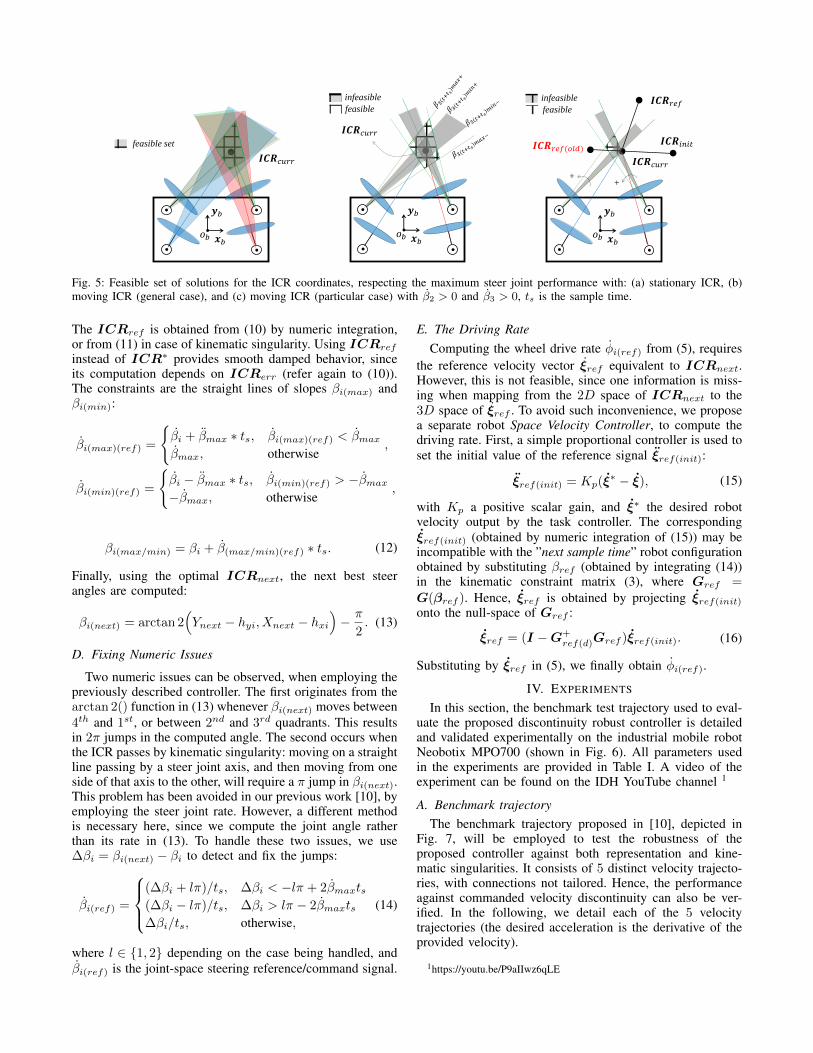
in computing the steer joint commands.Fig. 5 shows the feasible change, in one sample time

period ts, in each of the steer joints (in positive and negativedirections) based on: 1. the ICRcurr, and 2. the maximumsteer joint velocity and acceleration. Indeed, the feasibleset of ICRnext is within the intersection of the extremefeasible changes of all steer joints. The feasible region forICRnext shown in Fig. 5.a corresponds to a stationaryICRcurr, which can move arbitrarily in any direction withinthe indicated feasible set. Instead, Fig. 5.b depicts the caseof moving ICRcurr (i.e., ˙ICRcurr 6= 0). In such case,the maximum steering deceleration constraints (shown inFig. 5.b as βi(t+ts)min+ and βi(t+ts)min− for minimumchange in steer angle in positive and negative directions,respectively) will apply, to further restrict the feasible set,dividing it into four regions based on the current steer ratedirection. Figure 5.c shows a particular case of Fig. 5.bwhere β2 > 0 and β3 > 0. Also, the case of discontinuouschange in the desired motion trajectory is depicted, wherea new reference ICR point ICRref appeared while theICRcurr is following an old one ICRref(old). Thanks tothis approach, discontinuity in velocity command can behandled seamlessly with the same formulation, and no steerjoint reconfiguration is needed.

All cases can be addressed by formulating a quadratic opti-mization problem, subject to linear constraints, to minimizethe error between the ICR reference signal ICRref andthe best feasible ICR at the next sample time ICRnext =[Xnext Ynext

]T, being also the decision variable:

minimizeICRnext

‖ICRref − ICRnext‖22subject to (−1)qi(min)Ai(min)(ICRnext − hi) ≥ 0,

(−1)qi(max)+1Ai(max)(ICRnext − hi) ≤ 0,

where ‖∗‖22 is the squared Euclidean norm, Ai(max/min) =[cot(βi(max/min)) 1

], hi =

[hxi hyi

]T, and qi(max/min)

is a parameter indicating the βi(max/min) quadrature:

qi(max/min) =

{0, if βi(max/min) ∈ 1st ∨ 4thquadrant,1, if βi(max/min) ∈ 2nd ∨ 3rdquadrant.

𝒙𝑏

𝒚𝑏

𝑜𝑏

𝑰𝑪𝑹𝑐𝑢𝑟𝑟

infeasible

feasible

𝒙𝑏

𝒚𝑏

𝑜𝑏

𝑰𝑪𝑹𝑐𝑢𝑟𝑟

feasible set

𝒙𝑏

𝒚𝑏

𝑜𝑏

𝑰𝑪𝑹𝑐𝑢𝑟𝑟

infeasible

feasible

+ +

𝑰𝑪𝑹𝑟𝑒𝑓

𝑰𝑪𝑹𝑟𝑒𝑓(𝑜𝑙𝑑) 𝑰𝑪𝑹𝑖𝑛𝑖𝑡

Fig. 5: Feasible set of solutions for the ICR coordinates, respecting the maximum steer joint performance with: (a) stationary ICR, (b)moving ICR (general case), and (c) moving ICR (particular case) with β2 > 0 and β3 > 0, ts is the sample time.

The ICRref is obtained from (10) by numeric integration,or from (11) in case of kinematic singularity. Using ICRref

instead of ICR∗ provides smooth damped behavior, sinceits computation depends on ICRerr (refer again to (10)).The constraints are the straight lines of slopes βi(max) andβi(min):

βi(max)(ref) =

{βi + βmax ∗ ts, βi(max)(ref) < βmaxβmax, otherwise

,

βi(min)(ref) =

{βi − βmax ∗ ts, βi(min)(ref) > −βmax−βmax, otherwise

,

βi(max/min) = βi + β(max/min)(ref) ∗ ts. (12)

Finally, using the optimal ICRnext, the next best steerangles are computed:

βi(next) = arctan 2(Ynext − hyi, Xnext − hxi

)− π

2. (13)

D. Fixing Numeric Issues

Two numeric issues can be observed, when employing thepreviously described controller. The first originates from thearctan 2() function in (13) whenever βi(next) moves between4th and 1st, or between 2nd and 3rd quadrants. This resultsin 2π jumps in the computed angle. The second occurs whenthe ICR passes by kinematic singularity: moving on a straightline passing by a steer joint axis, and then moving from oneside of that axis to the other, will require a π jump in βi(next).This problem has been avoided in our previous work [10], byemploying the steer joint rate. However, a different methodis necessary here, since we compute the joint angle ratherthan its rate in (13). To handle these two issues, we use∆βi = βi(next) − βi to detect and fix the jumps:

βi(ref) =

(∆βi + lπ)/ts, ∆βi < −lπ + 2βmaxts(∆βi − lπ)/ts, ∆βi > lπ − 2βmaxts∆βi/ts, otherwise,

(14)

where l ∈ {1, 2} depending on the case being handled, andβi(ref) is the joint-space steering reference/command signal.

E. The Driving RateComputing the wheel drive rate φi(ref) from (5), requires

the reference velocity vector ξref equivalent to ICRnext.However, this is not feasible, since one information is miss-ing when mapping from the 2D space of ICRnext to the3D space of ξref . To avoid such inconvenience, we proposea separate robot Space Velocity Controller, to compute thedriving rate. First, a simple proportional controller is used toset the initial value of the reference signal ξref(init):

ξref(init) = Kp(ξ∗ − ξ), (15)

with Kp a positive scalar gain, and ξ∗ the desired robotvelocity output by the task controller. The correspondingξref(init) (obtained by numeric integration of (15)) may beincompatible with the ”next sample time” robot configurationobtained by substituting βref (obtained by integrating (14))in the kinematic constraint matrix (3), where Gref =G(βref ). Hence, ξref is obtained by projecting ξref(init)onto the null-space of Gref :

ξref = (I −G+ref(d)Gref )ξref(init). (16)

Substituting by ξref in (5), we finally obtain φi(ref).

IV. EXPERIMENTS

In this section, the benchmark test trajectory used to eval-uate the proposed discontinuity robust controller is detailedand validated experimentally on the industrial mobile robotNeobotix MPO700 (shown in Fig. 6). All parameters usedin the experiments are provided in Table I. A video of theexperiment can be found on the IDH YouTube channel 1

A. Benchmark trajectoryThe benchmark trajectory proposed in [10], depicted in

Fig. 7, will be employed to test the robustness of theproposed controller against both representation and kine-matic singularities. It consists of 5 distinct velocity trajecto-ries, with connections not tailored. Hence, the performanceagainst commanded velocity discontinuity can also be ver-ified. In the following, we detail each of the 5 velocitytrajectories (the desired acceleration is the derivative of theprovided velocity).

1https://youtu.be/P9aIIwz6qLE

Fig. 6: Photograph of the Neobotix MPO700 industrial SWMR.

1) Parabolic ICR position profile: This test excites steerjoint motion in the vicinity of kinematic singularity, to checkif it will respect the joint limits. A parabolic ICR-pointmotion with vertex at one of the steering axes is used, andimplemented smoothly using a constant velocity profile: x∗ = 0.5 ∗ (2y + hx2)2 + hy2

y∗ = Tc4b(yi = 0, yf = −hx2, ti = 2, tf = 6, t)

θ∗ = 0.5.(17)

Here, Tc4b is a 4th order trajectory, taking initial velocity yi,final velocity yf , initial time ti, final time tf , and currenttime t as arguments:

Tc4b =

a0 + a1δt1 + a2δt

21 + a3δt

31 + a4δt

41, ti ≤ t < t1

a5, t1 ≤ t < t2

a0 + a1δt3 + a2δt23 + a3δt

33 + a4δt

43, t2 ≤ t < tf .

Coefficients a0 ... a5, are computed by setting the initial andfinal acceleration/jerk (boundary conditions) to zero, δt1 =t− ti, δt2 = t− t1, and δt3 = t− t2, while t1 = ti + 0.1 ∗(tf − ti), and t2 = tf − 0.1 ∗ (tf − ti). Before employingthe velocity profile in (17), the following velocity commandis applied, to guarantee that the parabolic ICR profile startsat the correct initial condition:

ξ∗ = 0.5 ∗[h2x2 + hy2 0 1

]T, 0 ≤ t < 2.

2) ICR point at kinematic singularity: This test reveals thebehavior of the steer joint exactly at kinematic singularity.Will it respect the maximum steer joint performance limits?Will it keep operating at the maximum limits or move at”low” velocity? The latter is preferable, in terms of energyconsumption and hardware safety. We used:

ξ∗ = 0.5 ∗[hy1 −hx1 1

]T, 6 ≤ t < 8.

TABLE I: Robot and Controller parameters used in the experiments.

a 0.19m b 0.24m d 0.045mrw 0.09m δ 0.001 R∞ 10m

δ1 1−9 Vmax 10m/s βth 0.005rad.

λ 3.7 Rzone 0.015m βmax 2rad./s

βmax 25rad./s2 ts 25ms Kp 2

𝒙𝑏

𝒚𝑏

𝑜𝑏

𝐼𝐶𝑅 ③ ICR at infinity

① Parabolic

ICR passing by

the steer axis

② ICR at the

steer axis

④ Straight ICR

profile between

steering axes

⑤ Zero base

frame velocity

Fig. 7: Schematic model of the 5 benchmark test trajectories.

3) Pure linear motion: Tests the robustness against repre-sentational singularity in ICR-based models and controllers,that usually employ θ in the denominator, by sending ”zeroangular velocity” and arbitrary linear velocity var:

ξ∗ =[var1 var2 0

]T, 8 ≤ t < 10.

4) Straight line motion of the ICR between steering axes:Consists in moving the ICR along a straight line connectingany two steering axes (i.e., six straight lines for the 4 SWMR).This tests the performance of Cartesian space kinematicmodels, developed using only two steerable wheels, sincean ICR motion on the line connecting them will result inundefined motion for the other steering joints. This test isrealized by the following command sequence:

ξ∗ = 0.5 ∗[hy1 −hx1 1

]T, 10 ≤ t < 12,

ξ∗ = 0.5 ∗[hy2 −hx2 1

]T, 12 ≤ t < 14,

ξ∗ = 0.5 ∗[hy3 −hx3 1

]T, 14 ≤ t < 16,

ξ∗ = 0.5 ∗[hy4 −hx4 1

]T, 16 ≤ t < 18,

ξ∗ = 0.5 ∗[hy2 −hx2 1

]T, 18 ≤ t < 20,

ξ∗ = 0.5 ∗[hy1 −hx1 1

]T, 20 ≤ t < 22,

ξ∗ = 0.5 ∗[hy4 −hx4 1

]T, 22 ≤ t < 24,

ξ∗ = 0.5 ∗[hy3 −hx3 1

]T, 24 ≤ t < 26,

ξ∗ = 0.5 ∗[hy1 −hx1 1

]T, 26 ≤ t < 28.

5) Zero Velocity: Tests the robustness against representa-tion singularity in Cartesian velocity based models employ-ing x, y, and θ in the denominator of (4). We use:

ξ∗ =[0 0 0

]T, 28 ≤ t < 30.

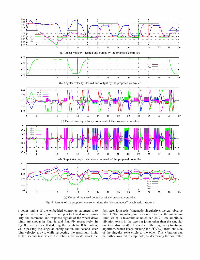
B. Results and DiscussionApplying the benchmark test trajectory shown in Fig. 8a

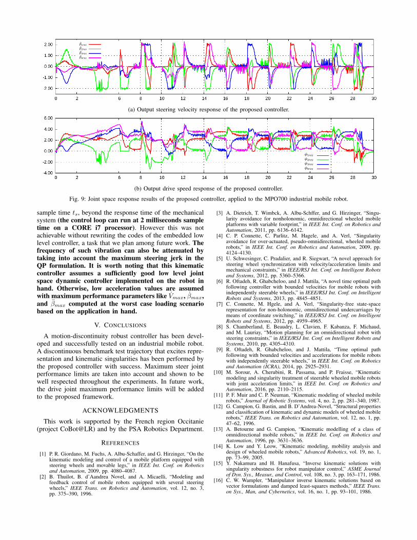
and Fig. 8b to the proposed controller, we obtain the steerjoint velocity and acceleration commands in Fig. 8c andFig. 8d, respectively. As shown, these commands respectthe maximum joint performance limits. The correspondingCartesian space velocity is also shown in Fig. 8a and Fig.8b, where a deviation from the trajectory is autonomouslyperformed to accommodate for the ”planned discontinuity”.When implemented on the Neobotix-MPO700, the steer jointvelocity response is obtained as in Fig. 9a, showing someovershoot due to imperfect embedded controller. However,

𝑥 ∗ 𝑦 ∗ 𝑥 𝑟𝑒𝑓

𝑥 𝑟𝑒𝑓

(a) Linear velocity: desired and output by the proposed controller.

𝜃 ∗

𝜃 𝑟𝑒𝑓

(b) Angular velocity: desired and output by the proposed controller.

𝛽 1𝑟𝑒𝑓

𝛽 2𝑟𝑒𝑓

𝛽 3𝑟𝑒𝑓

𝛽 4𝑟𝑒𝑓

(c) Output steering velocity command of the proposed controller.

𝛽 1𝑟𝑒𝑓

𝛽 2𝑟𝑒𝑓

𝛽 3𝑟𝑒𝑓

𝛽 4𝑟𝑒𝑓

(d) Output steering acceleration command of the proposed controller.

𝜑 1𝑟𝑒𝑓

𝜑 2𝑟𝑒𝑓 𝜑 3𝑟𝑒𝑓

𝜑 4𝑟𝑒𝑓

(e) Output drive speed command of the proposed controller.

Fig. 8: Results of the proposed controller along the “discontinuous” benchmark trajectory.

a better tuning of the embedded controller parameters, toimprove the response, is still an open technical issue. Simi-larly, the command and response signals of the wheel drivejoints are shown in Fig. 8e and Fig. 9b, respectively. InFig. 8c, we can see that during the parabolic ICR motion,while passing the singular configuration, the second steerjoint velocity grows, while respecting the maximum limit.In the second test where the robot must rotate about the

first steer joint axis (kinematic singularity), we can observethat: 1. The singular joint does not rotate at the maximumlimit, which is favorable as noted earlier, 2. Low amplitudevibration exists in the steering joints other than the singularone (see also test 4). This is due to the singularity treatmentalgorithm, which keeps pushing the ICRref from one sideof the singular zone circle to the other. This vibration canbe further lowered in amplitude, by decreasing the controller

𝛽 1𝑟𝑒𝑠

𝛽 2𝑟𝑒𝑠 𝛽 3𝑟𝑒𝑠

𝛽 4𝑟𝑒𝑠

(a) Output steering velocity response of the proposed controller.

𝜑 1𝑟𝑒𝑠 𝜑 2𝑟𝑒𝑠 𝜑 3𝑟𝑒𝑠 𝜑 4𝑟𝑒𝑠

(b) Output drive speed response of the proposed controller.

Fig. 9: Joint space response results of the proposed controller, applied to the MPO700 industrial mobile robot.

sample time ts, beyond the response time of the mechanicalsystem (the control loop can run at 2 milliseconds sampletime on a CORE i7 processor). However this was notachievable without rewriting the codes of the embedded lowlevel controller, a task that we plan among future work. Thefrequency of such vibration can also be attenuated bytaking into account the maximum steering jerk in theQP formulation. It is worth noting that this kinematiccontroller assumes a sufficiently good low level jointspace dynamic controller implemented on the robot inhand. Otherwise, low acceleration values are assumedwith maximum performance parameters like Vmax, βmax,and βmax computed at the worst case loading scenariobased on the application in hand.

V. CONCLUSIONS

A motion-discontinuity robust controller has been devel-oped and successfully tested on an industrial mobile robot.A discontinuous benchmark test trajectory that excites repre-sentation and kinematic singularities has been performed bythe proposed controller with success. Maximum steer jointperformance limits are taken into account and shown to bewell respected throughout the experiments. In future work,the drive joint maximum performance limits will be addedto the proposed framework.

ACKNOWLEDGMENTS

This work is supported by the French region Occitanie(project CoBot@LR) and by the PSA Robotics Department.

REFERENCES

[1] P. R. Giordano, M. Fuchs, A. Albu-Schaffer, and G. Hirzinger, “On thekinematic modeling and control of a mobile platform equipped withsteering wheels and movable legs,” in IEEE Int. Conf. on Roboticsand Automation, 2009, pp. 4080–4087.

[2] B. Thuilot, B. d’Aandrea Novel, and A. Micaelli, “Modeling andfeedback control of mobile robots equipped with several steeringwheels,” IEEE Trans. on Robotics and Automation, vol. 12, no. 3,pp. 375–390, 1996.

[3] A. Dietrich, T. Wimbck, A. Albu-Schffer, and G. Hirzinger, “Singu-larity avoidance for nonholonomic, omnidirectional wheeled mobileplatforms with variable footprint,” in IEEE Int. Conf. on Robotics andAutomation, 2011, pp. 6136–6142.

[4] C. P. Connette, C. Parlitz, M. Hagele, and A. Verl, “Singularityavoidance for over-actuated, pseudo-omnidirectional, wheeled mobilerobots,” in IEEE Int. Conf. on Robotics and Automation, 2009, pp.4124–4130.

[5] U. Schwesinger, C. Pradalier, and R. Siegwart, “A novel approach forsteering wheel synchronization with velocity/acceleration limits andmechanical constraints,” in IEEE/RSJ Int. Conf. on Intelligent Robotsand Systems, 2012, pp. 5360–5366.

[6] R. Oftadeh, R. Ghabcheloo, and J. Mattila, “A novel time optimal pathfollowing controller with bounded velocities for mobile robots withindependently steerable wheels,” in IEEE/RSJ Int. Conf. on IntelligentRobots and Systems, 2013, pp. 4845–4851.

[7] C. Connette, M. Hgele, and A. Verl, “Singularity-free state-spacerepresentation for non-holonomic, omnidirectional undercarriages bymeans of coordinate switching,” in IEEE/RSJ Int. Conf. on IntelligentRobots and Systems, 2012, pp. 4959–4965.

[8] S. Chamberland, E. Beaudry, L. Clavien, F. Kabanza, F. Michaud,and M. Lauriay, “Motion planning for an omnidirectional robot withsteering constraints,” in IEEE/RSJ Int. Conf. on Intelligent Robots andSystems, 2010, pp. 4305–4310.

[9] R. Oftadeh, R. Ghabcheloo, and J. Mattila, “Time optimal pathfollowing with bounded velocities and accelerations for mobile robotswith independently steerable wheels,” in IEEE Int. Conf. on Roboticsand Automation (ICRA), 2014, pp. 2925–2931.

[10] M. Sorour, A. Cherubini, R. Passama, and P. Fraisse, “Kinematicmodeling and singularity treatment of steerable wheeled mobile robotswith joint acceleration limits,” in IEEE Int. Conf. on Robotics andAutomation, 2016, pp. 2110–2115.

[11] P. F. Muir and C. P. Neuman, “Kinematic modeling of wheeled mobilerobots,” Journal of Robotic Systems, vol. 4, no. 2, pp. 281–340, 1987.

[12] G. Campion, G. Bastin, and B. D’Andrea-Novel, “Structural propertiesand classification of kinematic and dynamic models of wheeled mobilerobots,” IEEE Trans. on Robotics and Automation, vol. 12, no. 1, pp.47–62, 1996.

[13] A. Betourne and G. Campion, “Kinematic modelling of a class ofomnidirectional mobile robots,” in IEEE Int. Conf. on Robotics andAutomation, 1996, pp. 3631–3636.

[14] K. Low and Y. Leow, “Kinematic modeling, mobility analysis anddesign of wheeled mobile robots,” Advanced Robotics, vol. 19, no. 1,pp. 73–99, 2005.

[15] Y. Nakamura and H. Hanafusa, “Inverse kinematic solutions withsingularity robustness for robot manipulator control,” ASME Journalof Dyn. Sys., Measur., and Control, vol. 108, no. 3, pp. 163–171, 1986.

[16] C. W. Wampler, “Manipulator inverse kinematic solutions based onvector formulations and damped least-squares methods,” IEEE Trans.on Sys., Man, and Cybernetics, vol. 16, no. 1, pp. 93–101, 1986.