Motion Coordination with Distributed Information

Sonia Martınez Jorge Cortes Francesco Bullo

Think globally, act locallyRene J. Dubos, 1972

Introduction

Motion coordination is a remarkable phenomenon in biological systems and an extremelyuseful tool in man-made groups of vehicles, mobile sensors and embedded robotic systems.Just like animals do, groups of mobile autonomous agents need the ability to deploy overa given region, assume a specified pattern, rendezvous at a common point, or jointly movein a synchronized manner. These coordination tasks are typically to be achieved with littleavailable communication between the agents, and therefore, with limited information aboutthe state of the entire system.

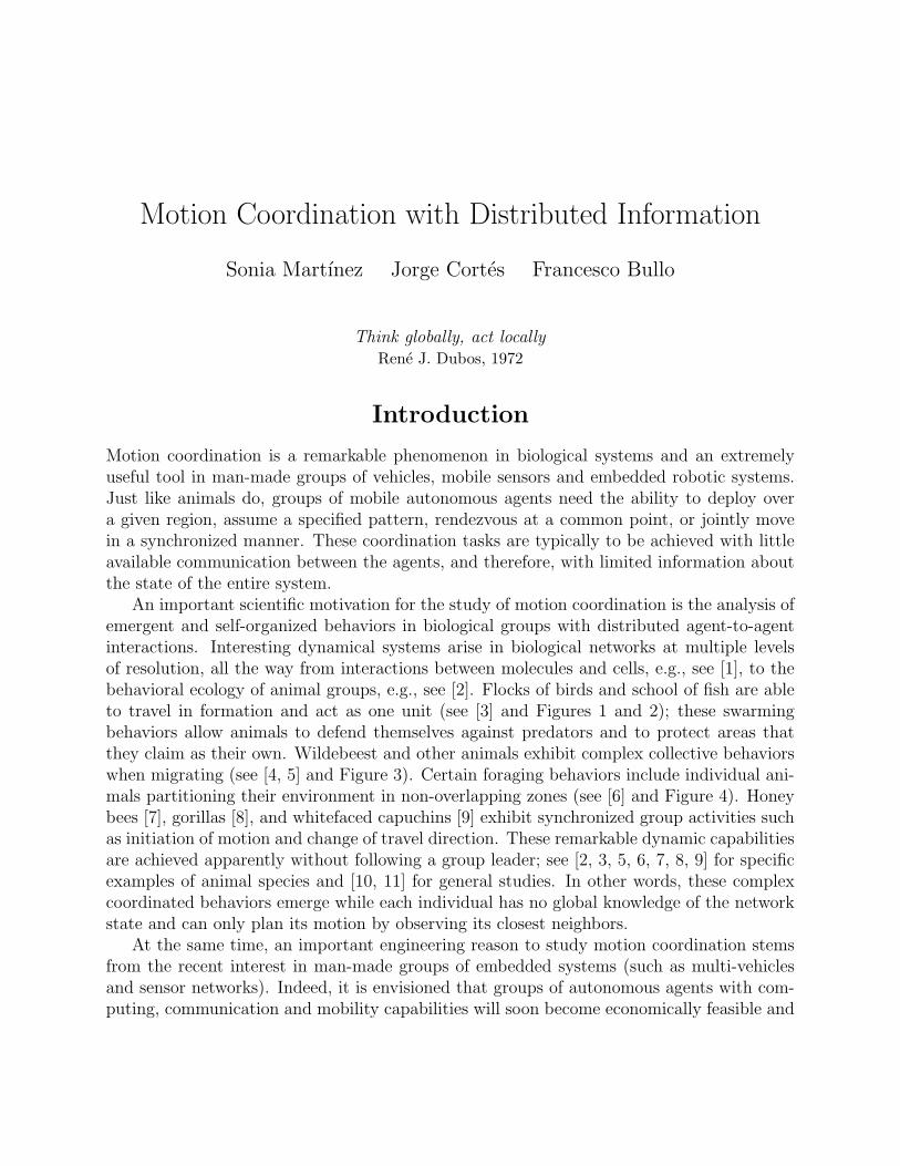
An important scientific motivation for the study of motion coordination is the analysis ofemergent and self-organized behaviors in biological groups with distributed agent-to-agentinteractions. Interesting dynamical systems arise in biological networks at multiple levelsof resolution, all the way from interactions between molecules and cells, e.g., see [1], to thebehavioral ecology of animal groups, e.g., see [2]. Flocks of birds and school of fish are ableto travel in formation and act as one unit (see [3] and Figures 1 and 2); these swarmingbehaviors allow animals to defend themselves against predators and to protect areas thatthey claim as their own. Wildebeest and other animals exhibit complex collective behaviorswhen migrating (see [4, 5] and Figure 3). Certain foraging behaviors include individual ani-mals partitioning their environment in non-overlapping zones (see [6] and Figure 4). Honeybees [7], gorillas [8], and whitefaced capuchins [9] exhibit synchronized group activities suchas initiation of motion and change of travel direction. These remarkable dynamic capabilitiesare achieved apparently without following a group leader; see [2, 3, 5, 6, 7, 8, 9] for specificexamples of animal species and [10, 11] for general studies. In other words, these complexcoordinated behaviors emerge while each individual has no global knowledge of the networkstate and can only plan its motion by observing its closest neighbors.

At the same time, an important engineering reason to study motion coordination stemsfrom the recent interest in man-made groups of embedded systems (such as multi-vehiclesand sensor networks). Indeed, it is envisioned that groups of autonomous agents with com-puting, communication and mobility capabilities will soon become economically feasible and

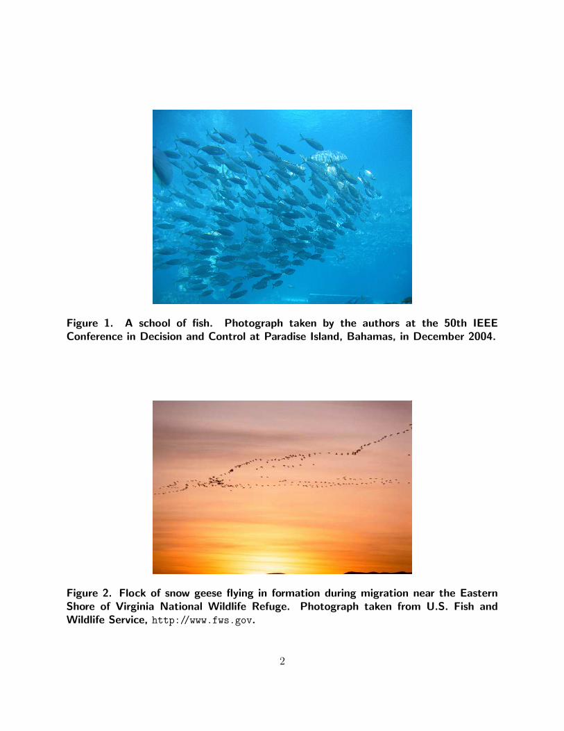
Figure 1. A school of fish. Photograph taken by the authors at the 50th IEEEConference in Decision and Control at Paradise Island, Bahamas, in December 2004.

Figure 2. Flock of snow geese flying in formation during migration near the EasternShore of Virginia National Wildlife Refuge. Photograph taken from U.S. Fish andWildlife Service, http://www.fws.gov.

2

Figure 3. Aerial photograph of a large wildebeest herd during the migration season onthe Serengeti National Park, Tanzania. Photograph taken from [4].

CENTROIDAL VORONOI TESSELLATIONS 649

Fig.2.2 A top-viewphotograph,usinga polarizing�lter,of theterritoriesof themale Tilapiamossambica;eachisa pitduginthesandbyitsoccupant.The boundariesoftheterritories,therimsofthepits,forma patternofpolygons.The breedingmalesare theblack�sh,whichrange in sizefrom about 15cm to 20cm. The gray �sh are thefemales,juveniles,andnonbreedingmales.The �shwitha conspicuousspotinitstail,intheupper-rightcorner,isa Cichlasomamaculicauda.Photographand captionreprinted from G. W. Barlow,HexagonalTerritories, Animal Behavior,Volume 22,1974,by permissionofAcademicPress,London.

As anexampleofsynchronoussettlingforwhich theterritoriescanbevisualized,considerthemouthbreeder�sh(Tilapiamossambica).Territorialmalesofthisspeciesexcavatebreedingpitsinsandybottomsby spittingsandaway fromthepitcenterstowardtheirneighbors.Fora highenoughdensity of�sh,thisreciprocalspittingresultsinsandparapetsthatarevisibleterritorialboundaries.In[3],theresultsofa controlledexperimentweregiven.Fishwereintroducedintoa largeoutdoorpoolwitha uniformsandybottom.Afterthe�shhad establishedtheirterritories,i.e.,afterthe�nalpositionsofthebreedingpitswereestablished,theparapetsseparatingtheterritorieswerephotographed.InFigure2.2,theresultingphotographfrom[3]isreproduced.The territoriesareseentobepolygonaland,in[27,59],itwasshownthattheyareverycloselyapproximatedby a Voronoitessellation.

A behavioralmodelforhow the�shestablishtheirterritorieswasgiven in[22,23,60].When the�shentera region,they�rstrandomlyselectthecentersoftheirbreedingpits,i.e.,thelocationsatwhich theywillspitsand.Theirdesiretoplacethepitcentersasfaraway aspossiblefromtheirneighborscausesthe�shtocontinuouslyadjustthepositionofthepitcenters.Thisadjustmentprocessismodeledasfollows.The�sh,intheirdesiretobeasfarawayaspossiblefromtheirneighbors,tendtomovetheirspittinglocationtowardthecentroidoftheircurrentterritory;subsequently,theterritorialboundariesm ustchangesincethe�sharespittingfromdi�erentlocations.Sinceallthe�shareassumedtobe ofequalstrength,i.e.,theyallpresumablyhave

Figure 4. Territorial behavior of fish. Top-view photograph of the territories of themale Tilapia mossambica; each is a pit dug in the sand by its occupant. The boundariesof the territories, the rims of the pits, form a pattern of polygons. The breeding malesare the black fish, which range in size from about 15cm to 20cm. The gray fish are thefemales, juveniles, and nonbreeding males. Photograph and caption taken from [6].

3

perform a variety of spatially-distributed sensing tasks such as search and rescue, surveil-lance, environmental monitoring, and exploration.

As a consequence of this growing interest, the research activity on cooperative con-trol has increased tremendously over the last few years. A necessarily incomplete list ofworks on distributed, or leaderless, motion coordination includes [12, 13, 14] on patternformation, [15, 16, 17] on flocking, [18] on self-assembly, [19] on swarm aggregation, [20] ongradient climbing, [21, 22, 23, 24] on deployment and task allocation, [25, 26, 27, 28] onrendezvous, [29, 30] on cyclic pursuit, [31] on vehicle routing and [32, 33, 34] on consen-sus. Heuristic approaches to the design of interaction rules and emergent behaviors havebeen thoroughly investigated within the literature on behavior-based robotics; see for exam-ple [35, 36, 37, 38].

The objective of this paper is to illustrate ways in which systems theory helps us analyzeemergent behaviors in animal groups and design autonomous and reliable robotic networks.We present and survey some recently-developed theoretical tools for modeling, analysis anddesign of motion coordination. We pay special attention to the following issues:

(i) in what sense is a coordination algorithm spatially distributed? To arrive at a satis-factory notion, we will resort to the concept of proximity graph from computationalgeometry [39]. Proximity graphs of different type model agent-to-agent interactionsthat depend only on the agents’ location in space. This is the case for example inwireless communication or in communication based on line-of-sight. Thus, the notionof proximity graph allows us to model the information flow between mobile agents;

(ii) how can we mathematically express motion coordination tasks? This is an importantquestion if we are interested in providing analytical guarantees for the performance ofcoordination algorithms. We will discuss various aggregate objective functions fromgeometric optimization for tasks such as deployment (via a class of multi-center func-tions that encode area-coverage, detection likelihood, and visibility coverage), ren-dezvous (via the diameter of convex hull function), cohesiveness, and agreement (viathe so-called Laplacian potential from algebraic graph theory). We also discuss theirsmoothness properties and identify their extreme points via nonsmooth analysis;

(iii) what tools are available to assess the performance of coordination algorithms? We willdiscuss a combination of system-theoretic and linear algebraic tools that are helpful inestablishing stability and convergence of motion coordination algorithms. This includesmethods from circulant and Toeplitz tridiagonal matrices and a recently-developed ver-sion of the LaSalle Invariance Principle for non-deterministic discrete-time dynamicalsystems;

(iv) finally, how can we design distributed coordination algorithms? We will build uponthe tools introduced earlier and present various approaches. A first approach is basedon the design of gradient flows: here we are typically given a coordination task tobe performed by the network and a proximity graph as communication constraint. Asecond approach is based on the analysis of emergent behaviors: in this case a notion

4

of neighboring agents and an interaction law between them is usually given. A thirdapproach is based on the identification of meaningful local objective functions whoseoptimization helps the network achieve the desired global task. The last and fourthapproach relies on the composition of basic behaviors. We apply these approaches tonumerous examples of coordination algorithms proposed in the literature.

Making sense of distributed

Our first goal is to provide a formally accurate notion of spatially distributed coordinationalgorithms. Roughly speaking, one would characterize an algorithm as distributed, as op-posed to centralized, if it relies on local information (instead of on global knowledge). Onecan find precise notions of distributed algorithms for networks with fixed topology in theliterature of automata theory and parallel computing [40]. Here, however, we are interestedin ad-hoc networks of mobile agents, where the topology changes dynamically, and thesedefinitions are not completely applicable. This motivates our current effort to arrive at asatisfactory definition of spatially distributed algorithms. In doing so, we will borrow thenotion of proximity graph from computational geometry. Before getting into this, let usrecall some basic geometric notions.

Basic geometric notions

A partition of a set S is a collection of subsets of S with disjoint interiors and whose unionis S. We denote by F(S) the collection of finite subsets of S. Given S ⊂ R

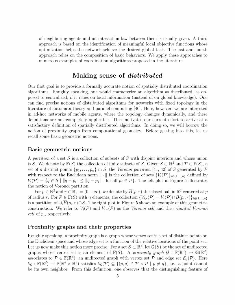
2 and P ∈ F(S), aset of n distinct points {p1, . . . , pn} in S, the Voronoi partition [41, 42] of S generated by Pwith respect to the Euclidean norm ‖ · ‖ is the collection of sets {Vi(P)}i∈{1,...,n} defined byVi(P) = {q ∈ S | ‖q − pi‖ ≤ ‖q − pj‖ , for all pj ∈ P}. The left plot in Figure 5 illustratesthe notion of Voronoi partition.

For p ∈ R2 and r ∈ R+ = (0, +∞), we denote by B(p, r) the closed ball in R

2 centered at pof radius r. For P ∈ F(S) with n elements, the collection {Vi,r(P) = Vi(P)∩B(pi, r)}i∈{1,...,n}

is a partition of ∪iB(pi, r)∩S. The right plot in Figure 5 shows an example of this geometricconstruction. We refer to Vi(P) and Vi,r(P) as the Voronoi cell and the r-limited Voronoicell of pi, respectively.

Proximity graphs and their properties

Roughly speaking, a proximity graph is a graph whose vertex set is a set of distinct points onthe Euclidean space and whose edge set is a function of the relative locations of the point set.Let us now make this notion more precise. For a set S ⊂ R

d, let G(S) be the set of undirectedgraphs whose vertex set is an element of F(S). A proximity graph G : F(Rd) → G(Rd)associates to P ∈ F(Rd), an undirected graph with vertex set P and edge set EG(P). HereEG : F(Rd) → F(Rd × R

d) satisfies EG(P) ⊆ {(p, q) ∈ P × P | p 6= q}, i.e., a point cannotbe its own neighbor. From this definition, one observes that the distinguishing feature of

5

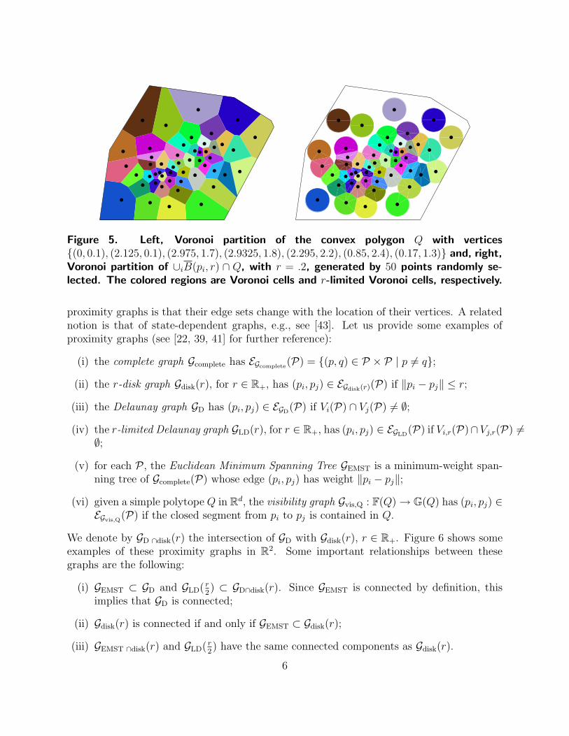
Figure 5. Left, Voronoi partition of the convex polygon Q with vertices{(0, 0.1), (2.125, 0.1), (2.975, 1.7), (2.9325, 1.8), (2.295, 2.2), (0.85, 2.4), (0.17, 1.3)} and, right,Voronoi partition of ∪iB(pi, r) ∩ Q, with r = .2, generated by 50 points randomly se-lected. The colored regions are Voronoi cells and r-limited Voronoi cells, respectively.

proximity graphs is that their edge sets change with the location of their vertices. A relatednotion is that of state-dependent graphs, e.g., see [43]. Let us provide some examples ofproximity graphs (see [22, 39, 41] for further reference):

(i) the complete graph Gcomplete has EGcomplete(P) = {(p, q) ∈ P × P | p 6= q};

(ii) the r-disk graph Gdisk(r), for r ∈ R+, has (pi, pj) ∈ EGdisk(r)(P) if ‖pi − pj‖ ≤ r;

(iii) the Delaunay graph GD has (pi, pj) ∈ EGD(P) if Vi(P) ∩ Vj(P) 6= ∅;

(iv) the r-limited Delaunay graph GLD(r), for r ∈ R+, has (pi, pj) ∈ EGLD(P) if Vi,r(P)∩Vj,r(P) 6=

∅;

(v) for each P , the Euclidean Minimum Spanning Tree GEMST is a minimum-weight span-ning tree of Gcomplete(P) whose edge (pi, pj) has weight ‖pi − pj‖;

(vi) given a simple polytope Q in Rd, the visibility graph Gvis,Q : F(Q) → G(Q) has (pi, pj) ∈

EGvis,Q(P) if the closed segment from pi to pj is contained in Q.

We denote by GD ∩disk(r) the intersection of GD with Gdisk(r), r ∈ R+. Figure 6 shows someexamples of these proximity graphs in R

2. Some important relationships between thesegraphs are the following:

(i) GEMST ⊂ GD and GLD( r2) ⊂ GD∩disk(r). Since GEMST is connected by definition, this

implies that GD is connected;

(ii) Gdisk(r) is connected if and only if GEMST ⊂ Gdisk(r);

(iii) GEMST ∩disk(r) and GLD( r2) have the same connected components as Gdisk(r).

6

PSfrag replacements

Delaunay

r-disk

Delaunay ∩ disk

r-lim. Delaunay

Gabriel

EMSTRel. Neigh.

x

y

z

PSfrag replacements

Delaunay

r-diskDelaunay ∩ disk

r-lim. Delaunay

Gabriel

EMSTRel. Neigh.

x

y

z

PSfrag replacements

Delaunay

r-diskDelaunay ∩ disk

r-lim. DelaunayGabriel

EMSTRel. Neigh.

x

y

z

PSfrag replacements

Delaunay

r-diskDelaunay ∩ disk

r-lim. Delaunay

GabrielEMST

Rel. Neigh.

x

y

z

Figure 6. From left to right, 2r-disk, Delaunay, r-limited Delaunay and EuclideanMinimum Spanning Tree graphs in R

2 for the point set in Figure 5, with r = .2.

In the case of graphs with a fixed topology, it is typical to alternatively describe the edgeset by means of the sets of neighbors of the individual graph vertices. Likewise, one canassociate to each proximity graph G, the set of neighbors map NG : R

d × F(Rd) → F(Rd)defined by

NG(p,P) = {q ∈ P | (p, q) ∈ EG(P ∪ {p})}.

Given p ∈ Rd, we will use the shorthand notation NG,p(P) = NG(p,P).

It is often the case that, if an agent has the information about the location of its neighborsdefined according to certain proximity graph, then it can compute its set of neighbors withrespect to a different proximity graph. For instance, if an agent knows the position of itsneighbors in the complete graph (i.e., of every other agent in the network), then it is clearthat it can compute its set of neighbors with respect to any proximity graph. Let us formalizethis idea. Given G1 and G2, we say that G1 is spatially distributed over G2 if, for all p ∈ P ,

NG1,p(P) = NG1,p

(NG2,p(P)

).

If G1 is spatially distributed over G2, then G1(P) ⊂ G2(P) for all P ∈ F(Rd). The converseis in general not true. For instance, GLD( r

2) is spatially distributed over Gdisk(r). On the

other hand, GD ∩disk is a subgraph of Gdisk, but it is not spatially distributed over it (see [22]for further details). Next, we build up on this discussion to provide a notion of spatiallydistributed map.

Spatially distributed maps

We are now ready to provide a formally accurate notion of spatially distributed map. Tosimplify the exposition, we will not distinguish notationally between a tuple in (p1, . . . , pn) ∈(Rd)n and its associated point set {p1, . . . , pn} ∈ F(Rd); we shall denote both quantities by P .The interested reader is referred to [28] for a detailed treatment in this regard.

Consider a map T : (Rd)n → Y n, with Y a given set. Let us denote by Tj the jthcomponent of T . We will say that T is spatially distributed over a proximity graph G ifthe jth component Tj evaluated at (p1, . . . , pn) can be computed with only the knowledge ofthe vertex pj and the neighboring vertices in G({p1, . . . , pn}). In mathematical terms, thisis expressed as follows:

7

The map T : (Rd)n → Y n is spatially distributed over G if there exist a mapT : R

d × F(Rd) → Y , with the property that, for all (p1, . . . , pn) ∈ (Rd)n and all

j ∈ {1, . . . , n}, one has Tj(p1, . . . , pn) = T (pj,NG,pj({p1, . . . , pn})).

According to this definition, a proximity graph G1 is spatially distributed over a proximitygraph G2 if and only if the set of neighbors map NG1 is spatially distributed over G2. Later,when discussing various coordination algorithms, we will characterize them as being spatiallydistributed with regards to appropriate proximity graphs.

Encoding coordination tasks

Our second goal is to develop mathematically sound methods to express motion coordinationtasks. In the following, we argue that aggregate behaviors of the entire mobile network canbe typically quantified by means of appropriately defined objective functions. Using toolsfrom geometric optimization, we will show how to encode various network objectives intolocational optimization functions. We will also pay special attention to the smoothnessproperties of these functions and the spatially distributed character of their gradients.

Aggregate objective functions for deployment

Loosely speaking, the deployment problem consists of placing a network of mobile agentsinside an environment of interest in order to achieve maximum coverage of it. Of course,“coverage” can be defined in many possible ways, as we illustrate in the following discussion.

Let Q ⊂ Rd be a simple convex polytope. A density function φ : Q → R+ is a bounded

measurable function. One can regard φ as a function measuring the probability that someevent takes place over the environment. A performance function f : R+ → R is a non-increasing and piecewise differentiable function with finite jump discontinuities. This func-tion describes the utility of placing an agent at a certain distance from a location in theenvironment. To illustrate this notion, consider a sensing scenario in which the agents areequipped with acoustic sensors that take measurements of sounds originating in the envi-ronment. Because of noise and loss of resolution, the ability to detect a sound originatingat a point q from the ith sensor at the position pi degrades with the distance ‖q − pi‖. Thisability is measured by the performance function f .

Given a density function φ and a performance function f , we are interested in maximizingthe expected value of the coverage performance provided by the group of agents over any pointin Q. To this end, let us define the function H : Qn → R by

H(P ) =

∫

Q

maxi∈{1,...,n}

f(‖q − pi‖)φ(q)dq. (1)

Note that H is an aggregate objective function since it depends on all the locations p1, . . . , pn.It will be of interest to find local maxima for H.

8

Different choices of performance function give rise to different aggregate objective func-tions with particular features. We now examine some important cases (let us remind thereader that {Vi(P )}i∈{1,...,n} and {Vi,R(P )}i∈{1,...,n} denote the Voronoi partition and thelimited-range Voronoi partition of Q generated by P ∈ (Rd)n, respectively):

Distortion problem: If f(x) = −x2, then H takes the form

HC(P ) = −n∑

i=1

∫

Vi(P )

‖q − pi‖2φ(q)dq = −

n∑

i=1

J(Vi(P ), pi),

where J(W, p) denotes the polar moment of inertia of the set W ⊂ Q about the point p.In signal compression −HC is referred to as the distortion function and is relevantin many disciplines including facility location, numerical integration, and clusteringanalysis, see [44].

Area problem: For a set S, let 1S denote the indicator function, 1S(q) = 1, if q ∈ S, and1S(q) = 0, if q 6∈ S. If f = 1[0,R], then H corresponds to the area, measured accordingto φ, covered by the union of the n balls B(p1, R), . . . , B(pn, R); that is,

Harea,R(P ) = areaφ(∪ni=1B(pi, R)) ,

where areaφ(S) =∫

Sφ(q)dq.

Mixed distortion-area problem: If f(x) = −x2 1[0,R](x) + b · 1(R,+∞)(x), for b ≤ −R2,then H takes the form

HR(P ) = −n∑

i=1

J(Vi,R(P ), pi) + b areaφ(Q \ ∪ni=1B(pi, R)) .

Aggregate objective functions for visibility-based deployment

Given a simple non-convex polytope Q in Rd and p ∈ Q, let S(p) = {q ∈ Q | [q, p] ⊂ Q}

denote the visible region in Q from the location p (here [q, p] is the closed segment from q top). Define

Hvis(P ) =

∫

Q

maxi∈{1,...,n}

1S(pi)(q)dq.

Roughly speaking, the function Hvis measures the amount of area of the non-convex polygonQ which is visible from any of the agents located at p1, . . . , pn. Therefore, it is of interestto find local maxima of Hvis. Note that one can also extend the definition of Hvis usinga density function φ : Q → R+, so that more importance is given to some regions of theenvironment being visible to the network (for instance, doors) than others.

9

Figure 7. Visible area to the network of a nonconvex environment, or equivalently,value of the function Hvis, at a given configuration (left, blue-colored region) and theunderlying visibility graph (right).

Aggregate objective functions for consensus

Let us consider a setup based on a fixed graph instead of a proximity graph. Let G =({1, . . . , n}, E) be an undirected graph with n vertices. The graph Laplacian matrix Lassociated with G (see, for instance, [45]) is defined by L = ∆ − A, where ∆ is the degreematrix and A is the adjacency matrix of the graph. The Laplacian matrix has some usefulproperties: it is symmetric, positive semi-definite and has λ = 0 as an eigenvalue witheigenvector (1, . . . , 1)T . More importantly, the graph G is connected if and only if rank(L) =n − 1, i.e., the eigenvalue 0 has algebraic multiplicity one. Following [32], we define thedisagreement function or Laplacian potential ΦG : R

n → R+ associated with G by

ΦG(x) = xT Lx =1

2

∑

(i,j)∈E

(xj − xi)2 .

For i ∈ {1, . . . , n}, the variable xi is associated with the agent pi. The variable xi mightrepresent physical quantities including heading, position, temperature, or voltage. Twoagents pi and pj are said to agree if and only if xi = xj. It is clear that ΦG(x) = 0 if and onlyif all neighboring nodes in the graph G agree. If, in addition, the graph G is connected, thenall nodes in the graph agree and a consensus is reached. Therefore, ΦG(x) is a meaningfulfunction that quantifies the group disagreement in a network.

Note that achieving consensus is a network coordination problem that does not necessarilyrefer to physical variables such as spatial coordinates or velocities. In what follows weconsider two “spatial versions” of consensus, that we refer to as rendezvous and cohesiveness.

Aggregate objective function for rendezvous

Roughly speaking, rendezvous means agreement over the location of the agents in a network.Let us define this notion more precisely. Recall that the convex hull co(S) of a set S ⊂ R

d

10

is the smallest convex set containing S. Additionally, the diameter of a set S is defined by

diam(S) = sup{‖p − q‖ | p, q ∈ S}.

With these two ingredients, we can now define the function Vdiam = diam ◦ co : (Rd)n → R+

by

Vdiam(P ) = diam(co(P )) = max{‖pi − pj‖ | i, j ∈ {1, . . . , n}}.

If diag((Rd)n) = {(p, . . . , p) ∈ (Rd)n | p ∈ Rd} denotes the diagonal set of (Rd)n, it is clear

that Vdiam(P ) = 0 if and only if P ∈ diag((Rd)n). Therefore, the set of global minima of Vdiam

corresponds to the network configurations where the agents rendezvous. One can also showthat Vdiam = diam ◦ co : (Rd)n → R+ is locally Lipschitz and invariant under permutationsof its arguments.

Aggregate objective functions for cohesiveness

Let us consider one final example of aggregate objective function that encodes a motioncoordination task. Let h : R+ → R be a continuously differentiable function satisfying thefollowing conditions: (i) limR→0+ h(R) = +∞, (ii) there exists R0 ∈ R+ such that h is convexon (0, R0) and concave on (R0, +∞), (iii) h achieves its minimum at all the points in theinterval [R∗, R

′∗] ⊂ (0, R0), and (iv) there exists R1 ≥ R0 such that h(R) = c for all R ≥ R1.

Figure 8 gives a particular example of a function h with these features.

PSfrag replacements

R∗ R′∗ R0 R1

Figure 8. Sample function h : R+ → R in the definition of the aggregate objectivefunctions for cohesiveness.

Let G be a proximity graph. Define the aggregate objective function

Hcohe,G(P ) =∑

(pi,pj)∈EG(P )

h(‖pi − pj‖) .

The minima of Hcohe,G correspond to “cohesive” network configurations. Specifically, forn ∈ {2, 3}, configurations that achieve the minimum value of Hcohe,G have all neighboring

11

agents’ locations within a distance contained in the interval [R∗, R′∗]. This objective function

and its variations have been employed over different proximity graphs in a number of works inthe literature ([19] and [20] over the complete graph, [16] over the r-disk graph) to guaranteecollision avoidance and cohesiveness of the mobile network.

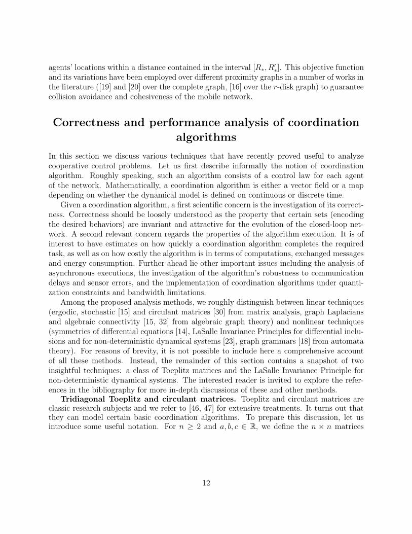
Correctness and performance analysis of coordination

algorithms

In this section we discuss various techniques that have recently proved useful to analyzecooperative control problems. Let us first describe informally the notion of coordinationalgorithm. Roughly speaking, such an algorithm consists of a control law for each agentof the network. Mathematically, a coordination algorithm is either a vector field or a mapdepending on whether the dynamical model is defined on continuous or discrete time.

Given a coordination algorithm, a first scientific concern is the investigation of its correct-ness. Correctness should be loosely understood as the property that certain sets (encodingthe desired behaviors) are invariant and attractive for the evolution of the closed-loop net-work. A second relevant concern regards the properties of the algorithm execution. It is ofinterest to have estimates on how quickly a coordination algorithm completes the requiredtask, as well as on how costly the algorithm is in terms of computations, exchanged messagesand energy consumption. Further ahead lie other important issues including the analysis ofasynchronous executions, the investigation of the algorithm’s robustness to communicationdelays and sensor errors, and the implementation of coordination algorithms under quanti-zation constraints and bandwidth limitations.

Among the proposed analysis methods, we roughly distinguish between linear techniques(ergodic, stochastic [15] and circulant matrices [30] from matrix analysis, graph Laplaciansand algebraic connectivity [15, 32] from algebraic graph theory) and nonlinear techniques(symmetries of differential equations [14], LaSalle Invariance Principles for differential inclu-sions and for non-deterministic dynamical systems [23], graph grammars [18] from automatatheory). For reasons of brevity, it is not possible to include here a comprehensive accountof all these methods. Instead, the remainder of this section contains a snapshot of twoinsightful techniques: a class of Toeplitz matrices and the LaSalle Invariance Principle fornon-deterministic dynamical systems. The interested reader is invited to explore the refer-ences in the bibliography for more in-depth discussions of these and other methods.

Tridiagonal Toeplitz and circulant matrices. Toeplitz and circulant matrices areclassic research subjects and we refer to [46, 47] for extensive treatments. It turns out thatthey can model certain basic coordination algorithms. To prepare this discussion, let usintroduce some useful notation. For n ≥ 2 and a, b, c ∈ R, we define the n × n matrices

12

Tridn(a, b, c) and Circn(a, b, c) by

Tridn(a, b, c) =

b c 0 . . . 0a b c . . . 0...

. . .. . .

. . ....

0 . . . a b c

0 . . . 0 a b

, Circn(a, b, c) = Tridn(a, b, c) +

0 . . . . . . 0 a

0 . . . . . . 0 0...

. . .. . .

. . ....

0 0 . . . 0 0c 0 . . . 0 0

.

Loosely speaking, we refer to Tridn and Circn as tridiagonal Toeplitz and circulant, respec-tively. These matrices appear in coordination problems where the communication networkhas the chain or the ring topology. For instance, the chain and the ring topology play an im-portant role in rendezvous problems [48] and in cyclic pursuit [29, 30] problems, respectively.In Figure 9, we illustrate two algorithms in which the control action of each agent dependson the location of its clockwise and counterclockwise neighbors. For both algorithms, the

umid

d coun

terclock

wise

dclockwise

pi+1

pi−1

pi

umid,V

Figure 9. Clockwise and counterclockwise neighbors of an agent in a network evolvingin S

1. Control laws such as “go towards the midpoint of the locations of the clockwiseand counterclockwise neighbors” (umid), or “go towards the midpoint of the Voronoisegment of the agent” (umid,V) give rise to linear dynamical systems described bycirculant matrices. In the closed-loop system determined by umid,V , the agents achieve auniform distribution along S

1. Oscillations instead persist when the law umid is adopted.

resulting linear dynamical system is determined by a circulant matrix.An important feature of tridiagonal Toeplitz and circulant matrices is that their eigen-

values and their dependency on n can be explicitly computed. The importance of this pointis illustrated by the following two example results from [48]. First, in certain rendezvousproblems, the closed-loop discrete-time trajectory x : N0 = N ∪ {0} → R

n satisfies

x(` + 1) = Tridn(a, b, c) x(`), x(0) = x0.

For the relevant case where a = c 6= 0 and |b| + 2|a| = 1, one can show not only thatlim`→+∞ x(`) = 0, but more importantly, that the maximum time required for ‖x(`)‖2 ≤

13

ε‖x0‖2 is of order n2 log ε−1, for ε ∈ (0, 1). Second, in deployment problems of the typedepicted in Figure 9, the closed-loop discrete-time trajectory y : N0 → R

n satisfies

y(` + 1) = Circn(a, b, c) y(`), y(0) = y0.

For the relevant case where a ≥ 0, c ≥ 0, b > 0, and a + b + c = 1, one can showthat lim`→+∞ y(`) = yave1, where yave = 1

n1T y0, and that the maximum time required for

‖y(`)− yave1‖2 ≤ ε‖y0 − yave1‖2 is again of order n2 log ε−1. (Here 1 = (1, . . . , 1)T .) The keypoint in these two examples is that stability and time complexity can be both establishedwhenever the tridiagonal Toeplitz and circulant structure is present.

LaSalle Invariance Principle for non-deterministic dynamical systems. Froma mathematical viewpoint, once a coordination algorithm for a networked control system isdesigned, or a particular interaction law modeling a biological behavior is identified, whatwe have is a set of coupled dynamical systems to analyze. Of course, the couplings betweenthe various dynamical systems change as the topology of the mobile network changes, andthis makes things intriguing and complicated at the same time. For instance, one oftenfaces issues such as discontinuity and non-smoothness of the vector fields modeling the evo-lution of the network. Other times, non-determinism arises because of asynchronism (forexample, to simplify the analysis of an algorithm, the asynchronous, deterministic evolutionof a mobile network may be subsumed into a larger set of synchronous, non-deterministicevolutions, see e.g., [26]), design choices when devising the coordination algorithm (at eachtime instant throughout the evolution, each agent may choose among multiple possible con-trol actions, as opposed to a single one, e.g., [22]) or communication, control and sensorerrors during the execution of the coordination algorithm (e.g., [25, 28]). Here we brieflysurvey a recently-developed LaSalle Invariance Principle for non-deterministic discrete-timedynamical systems.

Let P(Rd) denote the collection of subsets of Rd. For d ∈ N, let T : R

d → P(Rd) \ ∅ bea set-valued map (note that a map from R

d to Rd can be interpreted as a singleton-valued

map). A trajectory of T is a sequence {pm}m∈N0 ⊂ Rd with the property that

pm+1 ∈ T (pm) , m ∈ N0 .

In other words, given any initial p0 ∈ Rd, a trajectory of T is computed by recursively setting

pm+1 equal to an arbitrary element in T (pm). Therefore, T induces a non-deterministicdiscrete-time dynamical system [22, 49].

In order to study the stability of this type of discrete-time dynamical systems, we needto introduce a couple of new notions. According to [49], T is closed at p ∈ R

d if for all pairsof convergent sequences pk → p and p′k → p′ such that p′k ∈ T (pk), one has p′ ∈ T (p). Inparticular, every map T : R

d → Rd continuous at p ∈ R

d is closed at p. A set C is weaklypositively invariant with respect to T if, for any initial condition p0 ∈ C, there exists at leasta trajectory of T starting at p0 that remains in C, or equivalently, if there exists p ∈ T (p0)such that p ∈ C. Finally, a function V : R

d → R is non-increasing along T on W ⊂ Rd

if V (p′) ≤ V (p) for all p ∈ W and p′ ∈ T (p). We are ready to state the following resultfrom [22], see also [50].

14

Theorem 1 (LaSalle Invariance Principle for closed set-valued maps) Let T be a set-valuedmap closed at p, for all p ∈ W ⊂ R

d, and let V : Rd → R be a continuous function non-

increasing along T on W . Assume the trajectory {pm}m∈N0 of T takes values in W and isbounded. Then there exists c ∈ R such that

pm −→ M ∩ V −1(c) ,

where M is the largest weakly positively invariant set in {p ∈ W | ∃p′ ∈ T (p) with V (p′) =V (p)}.

Designing emergent behaviors

In this section, we elaborate on the role played by the tools introduced in the previous sectionsfor the design and analysis of motion coordination algorithms. We do not enter into technicaldetails throughout the discussion, but rather refer to various works for further reference. Ourintention is to provide a first step toward the establishment of a rigorous systems-theoreticapproach to motion coordination algorithms for a variety of spatially-distributed tasks.

Given a network of identical agents equipped with motion control and communicationcapabilities, the following subsections contain various approaches to the study of distributedand coordinated motions. Loosely speaking, a first approach is based on the design ofgradient flows : here a coordination task and a proximity graph are typically specified togetherwith a proximity graph imposing a communication constraint. A second approach is basedon the analysis of emergent behaviors : in this case a notion of neighboring agents and aninteraction law between them is usually given. A third approach is based on the identificationof meaningful local objective functions whose optimization helps the network achieve thedesired global task. Finally, the last and fourth approach relies on the composition of basicbehaviors.

Designing the coordination algorithm from the aggregate objective

function

The first step of this approach consists of identifying a global and aggregate objective func-tion which is relevant to the desired coordination task. Once this objective function isdetermined, one analyzes its differentiable properties and computes its (generalized) gradi-ent. With this information, it is possible to characterize its critical points, i.e. the desirednetwork configurations. The next step is to identify those proximity graphs that allow thecomputation of the gradient of the objective function in a spatially distributed manner. Ifany of these proximity graphs can be determined with the capabilities of the mobile network,then a control law for each agent simply consists of following the gradient of the aggregateobjective function. By the LaSalle Invariance Principle, such a coordination algorithm auto-matically guarantees convergence of the closed-loop network trajectories to the set of criticalpoints.

15

Example 1 (Distortion and area problems): The coordination algorithms for the distortionproblem and for the area problem proposed in [22] are examples of this approach. GivenQ a simple convex polygon in R

2 and R > 0, one can prove that the functions HC andHarea,R are locally Lipschitz on Qn and differentiable on Qn \ {(p1, . . . , pn) ∈ (R2)n | pi =pj for some i, j ∈ {1, . . . , n}, i 6= j}, with

∂HC

∂pi

(P ) = 2 M(Vi(P )) · (CM(Vi(P )) − pi) , (2a)

∂Harea,R

∂pi

(P ) =

∫

arc(Vi,R(P ))

nB(pi,R) φ , (2b)

where nB(p,R)(q) denotes the unit outward normal to B(p,R) at q ∈ ∂B(p,R) and, for eachi ∈ {1, . . . , n}, arc(∂Vi,R(P )) denotes the union of the arcs in ∂Vi,R(P ). The symbols M(W )and CM(W ) denote, respectively, the mass and the center of mass with respect to φ ofW ⊂ Q. The critical points P ∈ Qn of HC satisfy pi = CM(Vi(P )) for all i ∈ {1, . . . , n}.Such configurations are usually referred to as centroidal Voronoi configurations, see [44]. Thecritical points P ∈ Qn of Harea,R have the property that each pi is a local optimum for thearea covered by Vi,R = Vi ∩ B(pi, R) at fixed Vi. We will refer to such configurations asarea-centered Voronoi configurations.

From equation (2a) it is clear that the gradient of HC is spatially distributed over GD,whereas from equation (2b) one deduces that the gradient of Harea,R is spatially distributedover GLD(R). The gradient flows of HC and of Harea,R correspond to the coordination al-gorithms “move-toward-the-centroid of own Voronoi cell” and “move in the direction of the(weighted) normal to the boundary of own cell,” respectively. Figures 10 and 12 show anexample of the execution of these algorithms. Figures 11 and 13 illustrate the adaptiveproperties of these algorithms with respect to agent arrivals and departures. �

Figure 10. Distortion problem: 20 mobile agents in a convex polygon follow thegradient of HC (cf. equation (2a)). The density function φ (represented by means ofits contour plot) is the sum of four Gaussian functions. The left (respectively, right)figure illustrates the initial (respectively, the final) locations and Voronoi partition.The central figure illustrates the gradient descent flow.

16

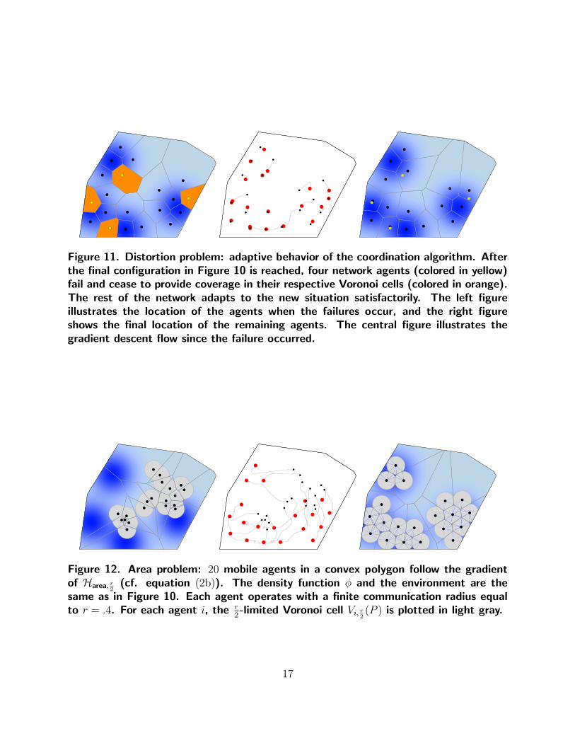
Figure 11. Distortion problem: adaptive behavior of the coordination algorithm. Afterthe final configuration in Figure 10 is reached, four network agents (colored in yellow)fail and cease to provide coverage in their respective Voronoi cells (colored in orange).The rest of the network adapts to the new situation satisfactorily. The left figureillustrates the location of the agents when the failures occur, and the right figureshows the final location of the remaining agents. The central figure illustrates thegradient descent flow since the failure occurred.

Figure 12. Area problem: 20 mobile agents in a convex polygon follow the gradientof Harea, r

2(cf. equation (2b)). The density function φ and the environment are the

same as in Figure 10. Each agent operates with a finite communication radius equalto r = .4. For each agent i, the r

2-limited Voronoi cell Vi, r

2(P ) is plotted in light gray.

17

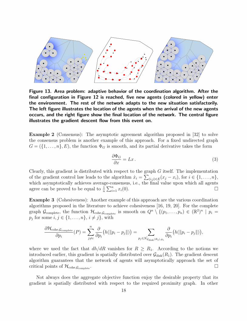
Figure 13. Area problem: adaptive behavior of the coordination algorithm. After thefinal configuration in Figure 12 is reached, five new agents (colored in yellow) enterthe environment. The rest of the network adapts to the new situation satisfactorily.The left figure illustrates the location of the agents when the arrival of the new agentsoccurs, and the right figure show the final location of the network. The central figureillustrates the gradient descent flow from this event on.

Example 2 (Consensus): The asymptotic agreement algorithm proposed in [32] to solvethe consensus problem is another example of this approach. For a fixed undirected graphG = ({1, . . . , n}, E), the function ΦG is smooth, and its partial derivative takes the form

∂ΦG

∂x= Lx . (3)

Clearly, this gradient is distributed with respect to the graph G itself. The implementationof the gradient control law leads to the algorithm xi =

∑(i,j)∈E(xj − xi), for i ∈ {1, . . . , n},

which asymptotically achieves average-consensus, i.e., the final value upon which all agentsagree can be proved to be equal to 1

n

∑n

i=1 xi(0). �

Example 3 (Cohesiveness): Another example of this approach are the various coordinationalgorithms proposed in the literature to achieve cohesiveness [16, 19, 20]. For the completegraph Gcomplete, the function Hcohe,Gcomplete

is smooth on Qn \ {(p1, . . . , pn) ∈ (R2)n | pi =pj for some i, j ∈ {1, . . . , n}, i 6= j}, with

∂Hcohe,Gcomplete

∂pi

(P ) =n∑

j 6=i

∂

∂pi

(h(‖pi − pj‖)

)=

∑

pj∈NGdisk(R1),pi

∂

∂pi

(h(‖pi − pj‖)

),

where we used the fact that dh/dR vanishes for R ≥ R1. According to the notions weintroduced earlier, this gradient is spatially distributed over Gdisk(R1). The gradient descentalgorithm guarantees that the network of agents will asymptotically approach the set ofcritical points of Hcohe,Gcomplete

. �

Not always does the aggregate objective function enjoy the desirable property that itsgradient is spatially distributed with respect to the required proximity graph. In other

18

words, given an available information flow, the corresponding gradient algorithm can notalways be computed. If this is the case, a possible approach is the following: (i) considerconstant-factor approximations of the objective function, (ii) identify those approximationswhose gradient is spatially distributed with respect to an appropriate proximity graph, and(iii) implement as coordination algorithm the one that makes each agent follow the gradientof the approximation.

Example 4 (Mixed distortion-area problem): The coordination algorithm proposed in [22]for the distortion problem falls into the situation described in the previous paragraph. Sincethe gradient of HC is spatially distributed over GD (cf. (2a)), and this graph is not spatiallydistributed over the r-disk graph, the coordination algorithm “move-toward-the-centroidof own Voronoi cell” is not implementable over a network with limited-range interactions.Instead, one can try to compute constant-factor approximations of HC. Indeed, for r ∈ R+,one has that (i) for β = r2/(2 diam Q)2,

H r2(P ) ≤ HC(P ) ≤ β H r

2(P ) < 0 , (4)

and (ii) the partial derivative of H r2

with respect to the position of the ith agent is

∂H r2

∂pi

(P ) = 2 M(Vi, r

2(P )

)·(

CM(Vi, r

2(P )

)− pi

)−

(r2

4+ b

) ∫

arc(∂Vi, r2(P ))

nB(pi,r2) φ ,

where we recall that arc(∂Vi, r2(P )) denotes the union of the arcs in ∂Vi, r

2(P ). Clearly, the

gradient of H r2

is spatially distributed over GLD( r2), and therefore, the coordination algorithm

based on the corresponding gradient control law is implementable over a network with r-limited interactions. Figure 14 illustrates the execution of this algorithm. �

Figure 14. Mixed distortion-area problem: 20 mobile agents in a convex polygon followthe gradient of H r

2. The density function φ and the environment are the same as in

Figure 10. Each agent operates with a finite radius r = .5. From the constant-factorapproximation (4), the absolute error is less than or equal to (β − 1)H r

2(Pfinal) ≈ 2.89,

where Pfinal denotes the final configuration of this execution. The percentage error inthe value of the HC at Pfinal with respect to the execution in Figure 10 is approximatelyequal to 4.24%.

19

Analyzing the coordinated behavior emerging from basic interac-

tion laws

This approach consists of devising a simple control law, typically inspired by some sortof heuristic, that implemented over each agent of the network would reasonably performthe desired task. Once this is done, one should (i) check that the resulting coordinationalgorithm is spatially distributed with regards to some appropriate proximity graph, and (ii)characterize its asymptotic convergence properties. One way of doing the latter is by findingan aggregate objective function that encodes the desired coordination task and by showingthat this function is optimized along the execution of the coordination algorithm.

Example 5 (Move-away-from-closest-neighbor): Consider the coordination algorithm stud-ied in [23] where each agent moves away from its closest neighbor (see Figure 15). This simpleinteraction law is spatially distributed over GD. One can prove that along the evolution ofthe network, the aggregate cost function

HSP(P ) = mini6=j∈{1,...,n}

{12‖pi − pj‖, dist(pi, ∂Q)

}, (5)

is monotonically non-decreasing. This function corresponds to the non-interference problem,where the network tries to maximize the coverage of the domain in such a way that the variouscommunication radius of the agents do not overlap or leave the environment (because ofinterference). Under appropriate technical conditions, one can show that the critical pointsof HSP are configurations where each agent is at the incenter of its own Voronoi region(recall that the incenter set of a polygon is the set of centers of the maximum-radius spherescontained in the polygon). �

Figure 15. Non-interference problem: “move-away-from-closest-neighbor” algorithmfor 16 mobile agents in a convex polygon. The left (respectively, right) figure illustratesthe initial (respectively, final) locations and Voronoi partition. The central figure illus-trates the network evolution. For each agent i, the ball of maximum radius containedin Vi(P ) and centered at pi is plotted in light gray.

Example 6 (Flocking): Consider the coordination algorithm analyzed in [15] for the flock-ing problem. Roughly speaking, flocking consists of agreeing over the direction of motion

20

by the agents in the network. Let G be a proximity graph. Now, consider the coordinationalgorithm where each agent performs the following steps: (i) detects its neighbors’ (accord-ing to G) heading; (ii) computes the average of its neighbors’ heading and its own heading,and (iii) updates its heading to the computed average. Clearly, this algorithm is spatiallydistributed over G. Moreover, assuming that G remains connected throughout the evolution,one can show that the agents asymptotically acquire the same heading. �

Designing the coordination algorithm from local objective functions

This approach has common elements with the two approaches presented previously. Now, inorder to derive a control law for each specific agent, one assumes that the neighboring agentsof that agent, or some spatial structure attributed to it, remain fixed. One then definesa local objective function, which is somehow related with the global aggregate objectivefunction encoding the desired coordination task, and devises a control law to optimize it. Thespecific control strategy might be heuristically derived or arise naturally from the gradientinformation of the local objective function. Once the coordination algorithm is set up, itshould be checked that it is spatially distributed and its asymptotic convergence propertiesshould be characterized.

Example 7 (Non-interference problem): Consider the aggregate objective function HSP

defined in equation (5). Consider the alternative expression,

HSP(P ) = mini∈{1,...,n}

smVi(P )(pi) ,

where smW (p) is the distance from p to the boundary of the convex polygon W , i.e., smW (p) =dist(p, ∂W ). Now, for i ∈ {1, . . . , n}, consider smVi(P ) as a local objective function. Assumingthat the Voronoi cell Vi(P ) remains fixed, then one can implement the (generalized) gradientascent of smVi(P ) as the control law for the agent pi. One can show [23] that this interactionlaw precisely corresponds to the strategy “move-away-from-closest-neighbor” discussed inExample 5. A related strategy consists of each agent moving toward the incenter of itsown Voronoi cell. The latter strategy can also be shown to make HSP monotonically non-decreasing and to enjoy analogous asymptotic convergence properties. �

Example 8 (Worst-case problem): Consider the aggregate objective function

HDC(P ) = maxq∈Q

{min

i∈{1,...,n}‖q − pi‖

}= max

i∈{1,...,n}lgVi(P )(pi) ,

where lgW (p) is the maximum distance from p to the boundary of the convex polygon W ,i.e., lgW (p) = maxq∈W ‖q − pi‖. Now, for i ∈ {1, . . . , n}, consider lgVi(P ) as a local objectivefunction. Assuming that the Voronoi cell Vi(P ) remains fixed, then one can implementthe (generalized) gradient descent of lgVi(P ) as the control law for the agent pi. One canshow [23] that this interaction law precisely corresponds to the strategy “move-toward-the-furthest-away-vertex-in-own-cell.” A related strategy consists of each agent moving toward

21

the circumcenter of its own Voronoi cell (recall that the circumcenter of a polygon is the centerof the minimum-radius sphere that contains it). Both strategies can be shown to make HDC

monotonically non-increasing and enjoy similar asymptotic convergence properties. Theseideas can be combined in other settings with different capabilities of the mobile agents, e.g.,in higher dimensional spaces (see Figure 16). �

Figure 16. Worst-case scenario: “move-toward-the-circumcenter” algorithm for 12mobile agents. Each agent illuminates a vertical cone with a fixed and common as-pect ratio. Each agent determines its Voronoi region within the planar polygon (thesame as in Figure 15) and then moves its horizontal position toward the circumcenterof its Voronoi cell and its vertical position to the minimal height spanning its ownVoronoi cell. The left (respectively, right) figure illustrates the initial (respectively,final) locations.

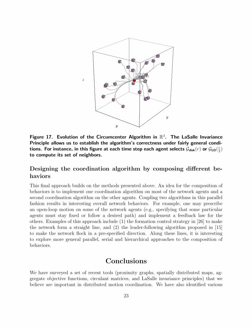
Example 9 (Rendezvous): Let G be a proximity graph. Consider the Circumcenter Al-gorithm over G, where each agent performs the following steps: (i) detects its neighborsaccording to G; (ii) computes the circumcenter of the point set comprised of its neighborsand of itself, and (iii) moves toward this circumcenter while maintaining connectivity withits neighbors. In order to maintain connectivity, the allowable motion of each agent is con-veniently restricted (see [25, 26, 28] for further details).

Note that with step (ii), assuming that all other agents remain fixed, each agent mini-mizes the local objective function given by the maximum distance from the agent to all itsneighbors in the proximity graph G. By construction, this coordination algorithm is spatiallydistributed over the proximity graph G. Moreover, one can prove that the evolution of theaggregate objective function Vdiam is monotonically non-increasing along the execution of theCircumcenter Algorithm. Using the LaSalle Invariance Principle for closed algorithms, onecan indeed characterize the asymptotic correctness properties of the Circumcenter Algorithmover G. See Figure 17 for an illustration of its execution. �

22

PSfrag replacements

xx

y

z

Figure 17. Evolution of the Circumcenter Algorithm in R3. The LaSalle Invariance

Principle allows us to establish the algorithm’s correctness under fairly general condi-tions. For instance, in this figure at each time step each agent selects Gdisk(r) or GLD( r

2)

to compute its set of neighbors.

Designing the coordination algorithm by composing different be-

haviors

This final approach builds on the methods presented above. An idea for the composition ofbehaviors is to implement one coordination algorithm on most of the network agents and asecond coordination algorithm on the other agents. Coupling two algorithms in this parallelfashion results in interesting overall network behaviors. For example, one may prescribean open-loop motion on some of the network agents (e.g., specifying that some particularagents must stay fixed or follow a desired path) and implement a feedback law for theothers. Examples of this approach include (1) the formation control strategy in [26] to makethe network form a straight line, and (2) the leader-following algorithm proposed in [15]to make the network flock in a pre-specified direction. Along these lines, it is interestingto explore more general parallel, serial and hierarchical approaches to the composition ofbehaviors.

Conclusions

We have surveyed a set of recent tools (proximity graphs, spatially distributed maps, ag-gregate objective functions, circulant matrices, and LaSalle invariance principles) that webelieve are important in distributed motion coordination. We have also identified various

23

approaches to the design of coordination algorithms and shown the wide applicability ofthe proposed tools in these approaches, see Table 1. We believe that the coming years willwitness an intense development of the field of distributed coordination and of its practicaluse in applications for multiple vehicles and sensor networks.

Agent motiondirection

Formal description Distributedinfo

Lyapunovfunction

Asymptoticconvergence

Ref.

centroid ofVoronoi cell

pi = CM(Vi(P )) − pi Voronoineighbors

HC centroidal Voronoiconfigurations

[21]

weighted aver-age normal ofr2-limited Voronoi

cell

pi =∫

arc(∂Vi, r2(P ))

nB(pi,r2) φ r-disk

neighborsHarea, r

2area-centeredVoronoi configu-rations

[22]

average of neigh-bors

pi =∑

j∈NG(i)(pj − pi) neighborsin fixed G

ΦG Consensus [32]

away from closestneighbor

pi = Ln(∂ smVi(P ))(P ) Voronoineighbors

HSP Incenter Voronoiconfigurations

[23]

furthest-away ver-tex in Voronoi cell

pi = −Ln(∂ lgVi(P ))(P ) Voronoineighbors

HDC CircumcenterVoronoi configu-rations

[23]

circumcenter ofneighbors’ andown position

pi(t+1) = pi(t)+λ∗i ·

(CC(Mi) − pi)r-diskneighbors

Vdiam rendezvous [25]

Table 1. Summary of example algorithms. In the interest of brevity, we refer to thecorresponding references for the notation employed.

Acknowledgments

This material is based upon work supported in part by ONR YIP Award N00014-03-1-0512and NSF SENSORS Award IIS-0330008. Sonia Martınez’s work was supported in part by aFulbright Postdoctoral Fellowship from the Spanish Ministry of Education and Science.

References

[1] M. B. Miller and B. L. Bassler, “Quorum sensing in bacteria,” Annual Review of Mi-crobiology, vol. 55, pp. 165–199, 2001.

[2] A. Okubo, “Dynamical aspects of animal grouping: swarms, schools, flocks and herds,”Advances in Biophysics, vol. 22, pp. 1–94, 1986.

[3] J. K. Parrish, S. V. Viscido, and D. Grunbaum, “Self-organized fish schools: an exami-nation of emergent properties,” Biological Bulletin, vol. 202, pp. 296–305, 2002.

24

[4] A. R. Sinclair, The African Buffalo, A Study of Resource Limitation of Population.Chicago, IL: The University of Chicago Press, 1977.

[5] S. Gueron and S. A. Levin, “Self-organization of front patterns in large wildebeestherds,” Journal of Theoretical Biology, vol. 165, pp. 541–552, 1993.

[6] G. W. Barlow, “Hexagonal territories,” Animal Behavior, vol. 22, pp. 876–878, 1974.

[7] T. D. Seeley and S. C. Buhrman, “Group decision-making in swarms of honey bees,”Behavioral Ecology and Sociobiology, vol. 45, pp. 19–31, 1999.

[8] K. J. Stewart and A. H. Harcourt, “Gorillas vocalizations during rest periods - signalsof impending departure,” Behaviour, vol. 130, pp. 29–40, 1994.

[9] S. Boinski and A. F. Campbell, “Use of trill vocalizations to coordinate troop movementamong whitefaced capuchins - a 2nd field-test,” Behaviour, vol. 132, pp. 875–901, 1995.

[10] I. D. Couzin, J. Krause, N. R. Franks, and S. A. Levin, “Effective leadership anddecision-making in animal groups on the move,” Nature, vol. 433, pp. 513–516, 2005.

[11] L. Conradt and T. J. Roper, “Group decision-making in animals,” Nature, vol. 421,no. 6919, pp. 155–158, 2003.

[12] I. Suzuki and M. Yamashita, “Distributed anonymous mobile robots: Formation ofgeometric patterns,” SIAM Journal on Computing, vol. 28, no. 4, pp. 1347–1363, 1999.

[13] C. Belta and V. Kumar, “Abstraction and control for groups of robots,” IEEE Trans-actions on Robotics, vol. 20, no. 5, pp. 865–875, 2004.

[14] E. W. Justh and P. S. Krishnaprasad, “Equilibria and steering laws for planar forma-tions,” Systems & Control Letters, vol. 52, no. 1, pp. 25–38, 2004.

[15] A. Jadbabaie, J. Lin, and A. S. Morse, “Coordination of groups of mobile autonomousagents using nearest neighbor rules,” IEEE Transactions on Automatic Control, vol. 48,no. 6, pp. 988–1001, 2003.

[16] H. Tanner, A. Jadbabaie, and G. J. Pappas, “Stability of flocking motion,” tech. rep.,Department of Computer and Information Science, University of Pennsylvania, Jan.2003.

[17] R. Olfati-Saber, “Flocking for multi-agent dynamic systems: Algorithms and theory,”IEEE Transactions on Automatic Control, 2005. To appear.

[18] E. Klavins, R. Ghrist, and D. Lipsky, “A grammatical approach to self-organizingrobotic systems,” IEEE Transactions on Automatic Control, 2005. To appear.

[19] V. Gazi and K. M. Passino, “Stability analysis of swarms,” IEEE Transactions onAutomatic Control, vol. 48, no. 4, pp. 692–697, 2003.

25

[20] P. Ogren, E. Fiorelli, and N. E. Leonard, “Cooperative control of mobile sensor net-works: adaptive gradient climbing in a distributed environment,” IEEE Transactionson Automatic Control, vol. 49, no. 8, pp. 1292–1302, 2004.

[21] J. Cortes, S. Martınez, T. Karatas, and F. Bullo, “Coverage control for mobile sensingnetworks,” IEEE Transactions on Robotics and Automation, vol. 20, no. 2, pp. 243–255,2004.

[22] J. Cortes, S. Martınez, and F. Bullo, “Spatially-distributed coverage optimization andcontrol with limited-range interactions,” ESAIM. Control, Optimisation & Calculus ofVariations, vol. 11, pp. 691–719, 2005.

[23] J. Cortes and F. Bullo, “Coordination and geometric optimization via distributed dy-namical systems,” SIAM Journal on Control and Optimization, June 2005. To appear.

[24] E. Frazzoli and F. Bullo, “Decentralized algorithms for vehicle routing in a stochastictime-varying environment,” in IEEE Conf. on Decision and Control, (Paradise Island,Bahamas), pp. 3357–3363, Dec. 2004.

[25] H. Ando, Y. Oasa, I. Suzuki, and M. Yamashita, “Distributed memoryless point con-vergence algorithm for mobile robots with limited visibility,” IEEE Transactions onRobotics and Automation, vol. 15, no. 5, pp. 818–828, 1999.

[26] J. Lin, A. S. Morse, and B. D. O. Anderson, “The multi-agent rendezvous problem: anextended summary,” in Proceedings of the 2003 Block Island Workshop on CooperativeControl (V. Kumar, N. E. Leonard, and A. S. Morse, eds.), vol. 309 of Lecture Notes inControl and Information Sciences, pp. 257–282, New York: Springer Verlag, 2004.

[27] Z. Lin, M. Broucke, and B. Francis, “Local control strategies for groups of mobileautonomous agents,” IEEE Transactions on Automatic Control, vol. 49, no. 4, pp. 622–629, 2004.

[28] J. Cortes, S. Martınez, and F. Bullo, “Robust rendezvous for mobile autonomous agentsvia proximity graphs in arbitrary dimensions,” IEEE Transactions on Automatic Con-trol, 2005. To appear.

[29] A. M. Bruckstein, N. Cohen, and A. Efrat, “Ants, crickets, and frogs in cyclic pursuit,”Tech. Rep. 9105, Technion – Israel Institute of Technology, Haifa, Israel, July 1991.Center for Intelligent Systems.

[30] J. A. Marshall, M. E. Broucke, and B. A. Francis, “Formations of vehicles in cyclicpursuit,” IEEE Transactions on Automatic Control, vol. 49, no. 11, pp. 1963– 1974,2004.

[31] V. Sharma, M. Savchenko, E. Frazzoli, and P. Voulgaris, “Time complexity of sensor-based vehicle routing,” in Robotics: Science and Systems, Cambridge, MA: MIT Press,2005. To appear.

26

[32] R. Olfati-Saber and R. M. Murray, “Consensus problems in networks of agents withswitching topology and time-delays,” IEEE Transactions on Automatic Control, vol. 49,no. 9, pp. 1520–1533, 2004.

[33] L. Moreau, “Stability of multiagent systems with time-dependent communication links,”IEEE Transactions on Automatic Control, vol. 50, no. 2, pp. 169–182, 2005.

[34] W. Ren and R. W. Beard, “Consensus seeking in multi-agent systems using dynamicallychanging interaction topologies,” IEEE Transactions on Automatic Control, vol. 50,no. 5, pp. 655–661, 2005.

[35] V. J. Lumelsky and K. R. Harinarayan, “Decentralized motion planning for multiplemobile robots: the cocktail party model,” Autonomous Robots, vol. 4, no. 1, pp. 121–135,1997.

[36] R. C. Arkin, Behavior-Based Robotics. Cambridge, MA: MIT Press, 1998.

[37] T. Balch and L. E. Parker, eds., Robot Teams: From Diversity to Polymorphism. Natick,MA: A K Peters Ltd., 2002.

[38] A. Howard, M. J. Mataric, and G. S. Sukhatme, “Mobile sensor network deploymentusing potential fields: A distributed scalable solution to the area coverage problem,”in International Conference on Distributed Autonomous Robotic Systems (DARS02),(Fukuoka, Japan), pp. 299–308, June 2002.

[39] J. W. Jaromczyk and G. T. Toussaint, “Relative neighborhood graphs and their rela-tives,” Proceedings of the IEEE, vol. 80, no. 9, pp. 1502–1517, 1992.

[40] N. A. Lynch, Distributed Algorithms. San Mateo, CA: Morgan Kaufmann Publishers,1997.

[41] M. de Berg, M. van Kreveld, M. Overmars, and O. Schwarzkopf, Computational Geom-etry: Algorithms and Applications. New York: Springer Verlag, 2 ed., 2000.

[42] A. Okabe, B. Boots, K. Sugihara, and S. N. Chiu, Spatial Tessellations: Concepts andApplications of Voronoi Diagrams. Wiley Series in Probability and Statistics, New York:John Wiley, 2 ed., 2000.

[43] M. Mesbahi, “On state-dependent dynamic graphs and their controllability properties,”IEEE Transactions on Automatic Control, vol. 50, no. 3, pp. 387–392, 2005.

[44] Q. Du, V. Faber, and M. Gunzburger, “Centroidal Voronoi tessellations: Applicationsand algorithms,” SIAM Review, vol. 41, no. 4, pp. 637–676, 1999.

[45] R. Diestel, Graph Theory, vol. 173 of Graduate Texts in Mathematics. New York:Springer Verlag, 2 ed., 2000.

27

[46] C. D. Meyer, Matrix Analysis and Applied Linear Algebra. Philadelphia, PA: SIAM,2001.

[47] P. J. Davis, Circulant Matrices. Providence, RI: American Mathematical Society, 2 ed.,1994.

[48] S. Martınez, F. Bullo, J. Cortes, and E. Frazzoli, “Synchronous robotic networks andcomplexity of control and communication laws,” Jan. 2005. Preprint. Available elec-tronically at http://xxx.arxiv.org/math.OC/0501499.

[49] D. G. Luenberger, Linear and Nonlinear Programming. Reading, MA: Addison-Wesley,2 ed., 1984.

[50] A. R. Teel, “Nonlinear systems: discrete-time stability analysis.” Lecture Notes, Uni-versity of California at Santa Barbara, 2004.

28