motion control of wheeled mobile robots - inria · 2009-09-30 · motion control of wheeled mobile...

Motion control of wheeled mobile robots

Pascal Morin and Claude Samson

INRIA

2004, Route des Lucioles

06902 Sophia-Antipolis Cedex, France

[email protected]

August 24, 2007

Contents

34 Motion control of wheeled mobile robots 1

34.1 Introduction . . . . . . . . . . . . . . . . . . . . . . . . . . . . . . . . . . . . . . . . . . . . . . . . . . 134.2 Control models . . . . . . . . . . . . . . . . . . . . . . . . . . . . . . . . . . . . . . . . . . . . . . . . 3

34.2.1 Kinematics versus dynamics . . . . . . . . . . . . . . . . . . . . . . . . . . . . . . . . . . . . . 334.2.2 Modeling in a Frenet frame . . . . . . . . . . . . . . . . . . . . . . . . . . . . . . . . . . . . . 4

34.3 Adaptation of control methods for holonomic systems . . . . . . . . . . . . . . . . . . . . . . . . . . 534.3.1 Stabilization of trajectories for a non-constrained point . . . . . . . . . . . . . . . . . . . . . 634.3.2 Path following with no orientation control . . . . . . . . . . . . . . . . . . . . . . . . . . . . . 6

34.4 Methods specific to nonholonomic systems . . . . . . . . . . . . . . . . . . . . . . . . . . . . . . . . . 734.4.1 Transformation of kinematic models into the chained form . . . . . . . . . . . . . . . . . . . . 834.4.2 Tracking of a reference vehicle with the same kinematics . . . . . . . . . . . . . . . . . . . . . 934.4.3 Path following with orientation control . . . . . . . . . . . . . . . . . . . . . . . . . . . . . . . 1234.4.4 Asymptotic stabilization of fixed postures . . . . . . . . . . . . . . . . . . . . . . . . . . . . . 1434.4.5 Limitations inherent to the control of nonholonomic systems . . . . . . . . . . . . . . . . . . 1934.4.6 Practical stabilization of arbitrary trajectories based on the transverse function approach . . 20

34.5 Complementary issues and bibliographical guide . . . . . . . . . . . . . . . . . . . . . . . . . . . . . 24

i

Chapter 34

Motion control of wheeled mobile robots

This chapter may be seen as a follow up to Chapter17, devoted to the classification and modeling of basicwheeled mobile robot (WMR) structures, and a natu-ral complement to Chapter 35, which surveys motionplanning methods for WMRs. A typical output of thesemethods is a feasible (or admissible) reference state-trajectory for a given mobile robot, and a question whichthen arises is how to make the physical mobile robottrack this reference trajectory via the control of the ac-tuators with which the vehicle is equipped. The objectof the present chapter is to bring elements of answer tothis question by presenting simple and effective controlstrategies. A first approach would consist in applyingopen-loop steering control laws like those developed inChapter 35. However, it is well known that this type ofcontrol is not robust to modeling errors (the sources ofwhich are numerous) and that it cannot guarantee thatthe mobile robot will move along the desired trajectoryas planned. This is why the methods here presented arebased on feedback control. Their implementation sup-poses that one is able to measure the variables involvedin the control loop (typically the position and orienta-tion of the mobile robot with respect to either a fixedframe or a path that the vehicle should follow). All alongthis chapter we will assume that these measurements areavailable continuously in time and that they are not cor-rupted by noise. In a general manner, robustness con-siderations will not be discussed in detail, a reason beingthat, beyond imposed space limitations, a large part ofthe presented approaches are based on linear control the-ory. The feedback control laws then inherit the strongrobustness properties associated with stable linear sys-tems. Results can also be subsequently refined by usingcomplementary, eventually more elaborated, automaticcontrol techniques.

34.1 Introduction

The control of wheeled mobile robots has been, and stillis, the subject of numerous research studies. In particu-lar, nonholonomy constraints associated with these sys-tems have motivated the development of highly nonlinearcontrol techniques. These approaches are addressed inthe present chapter, but their exposition is deliberatelylimited in order to give the priority to more classicaltechniques whose bases, both practical and theoretical,are better established.

For the sake of simplicity, the control methods aredeveloped mainly for unicycle-type and car-like mobilerobots, which correspond respectively to the types (2, 0)and (1, 1) in the classification proposed in Chapter 17.Most of the results can in fact be extended/adapted toother mobile robots, in particular to systems with trail-ers. We will mention the cases where such extensions arestraightforward. All reported simulation results, illus-trating various control problems and solutions, are car-ried out for a car-like vehicle whose kinematics is slightlymore complex than that of unicycle-type vehicles.

Recall (see Figure 34.1 below) that:

1. A unicycle-type mobile robot is schematicallycomposed of two independent actuated wheels ona common axle whose direction is rigidly linked tothe robot chassis, and one or several passively ori-entable –or caster– wheels, which are not controlledand serve for sustentation purposes.

2. A (rear-drive) car-like mobile robot is composedof a motorized wheeled-axle at the rear of the chas-sis, and one (or a pair of) orientable front steeringwheel(s).

Note also, as illustrated by the diagram below, that acar-like mobile robot can be viewed (at least kinemati-

1

CHAPTER 34. MOTION CONTROL OF WHEELED MOBILE ROBOTS 2

Figure 34.1: Unicycle-type and car-like mobile robots

cally) as a unicycle-type mobile robot to which a traileris attached.

φ φ

Figure 34.2: Analogy car / unicycle with trailer

Three generic control problems are studied in thischapter

Path following: Given a curve C on the plane, a (nonzero) longitudinal velocity v0 for the robot chassis, anda point P attached to the chassis, the goal is to have thepoint P follow the curve C when the robot moves with thevelocity v0. The variable that one has to stabilize at zerois thus the distance between the point P and the curve(i.e. the distance between P and the closest point M onC). This type of problem typically corresponds to drivingon a road while trying to maintain the distance betweenthe vehicle chassis and the side of the road constant.Automatic wall following is another possible application.

Stabilization of trajectories: This problem differsfrom the previous one in that the vehicle’s longitudi-nal velocity is no longer pre-determined because one alsoaims at monitoring the distance gone along the curveC. This objective supposes that the geometric curve Cis complemented with a time-schedule, i.e. that it isparametrized with the time variable t. This comes up todefining a trajectory t 7−→ (xr(t), yr(t)) with respect toa reference frame F0. Then the goal is to stabilize theposition error vector (x(t) − xr(t), y(t) − yr(t)) at zero,with (x(t), y(t)) denoting the coordinates of point P inF0 at time t. The problem may also be formulated as theone of controlling the vehicle in order to track a referencevehicle whose trajectory is given by t 7−→ (xr(t), yr(t)).Note that perfect tracking is achievable only if the ref-erence trajectory is feasible for the physical vehicle, and

that a trajectory which is feasible for a unicycle-typevehicle is not necessarily feasible for a car-like vehicle.Also, in addition to monitoring the position (x(t), y(t))of the robot, one may be willing to control the chassisorientation θ(t) at a desired reference value θr(t) associ-ated with the orientation of the reference vehicle. For anonholonomic unicycle-type robot, a reference trajectory(xr(t), yr(t), θr(t)) is feasible if it is produced by a ref-erence vehicle which has the same kinematic limitationsas the physical robot. For instance, most trajectoriesproduced by an omnidirectional vehicle (omnibile vehi-cle in the terminology of Chapter 17) are not feasible fora nonholonomic mobile robot. However, non-feasibilitydoes not imply that the reference trajectory cannot betracked in an approximate manner, i.e. with small (al-though non-zero) tracking errors. This justifies the intro-duction of a concept of practical stabilization, by opposi-tion to asymptotic stabilization when the tracking errorsconverge to zero. The last part of this chapter will be de-voted to a recent, and still prospective, control approachfor the practical stabilization of trajectories which arenot necessarily feasible.

Stabilization of fixed postures: Let F1 denote aframe attached to the robot chassis. In this chapter,we call a robot posture (or situation) the association ofthe position of a point P located on the robot chassiswith the orientation θ(t) of F1 with respect to a fixedframe F0 in the plane of motion. For this last problem,the objective is to stabilize at zero the posture vectorξ(t) = (x(t), y(t), θ(t)), with (x(t), y(t)) denoting the po-sition of P expressed in F0. Although a fixed desired(or reference) posture is obviously a particular case ofa feasible trajectory, this problem cannot be solved byclassical control methods.

The chapter is organized as follows. Section 34.2 isdevoted to the choice of control models and the determi-nation of modeling equations associated with the pathfollowing control problem. In Section 34.3, the problemsof path following and trajectory stabilization in positionare studied under an assumption upon the location of thepoint P chosen on the robot chassis. This assumptionimplies that the motion of this point is not constrained.It greatly simplifies the resolution of the considered prob-lems. However, a counterpart of this simplification isthat the stability of the robot’s orientation is not alwaysguaranteed, in particular during phases when the signof the robot’s longitudinal velocity is not constant. Theassumption upon P is removed in Section 34.4, and bothproblems are re-considered, together with the problem


of stabilizing a fixed posture. At the end of this sec-tion, a certain number of shortcomings and limitationsinherent to the objective of asymptotic stabilization arepointed out. They can be circumvented by consideringan objective of practical stabilization instead. Some ele-ments of a recent, and still prospective, control approachdeveloped with this point of view –based on the use ofso-called transverse functions– are presented in the Sec-tion 34.4.6. Finally, a few complementary issues on thefeedback control of mobile robots are shortly discussedin the concluding Section 34.5, with a list of commentedreferences for further reading on WMR motion control.

34.2 Control models

34.2.1 Kinematics versus dynamics

Relation (17.29) in Chapter 17 provides a general config-uration dynamic model for WMRs. Its particularizationto the case of unicycle-type and car-like mobile robotsgives

H(q)u+ F (q, u)u = Γ(φ)τ (34.1)

with q denoting a robot’s configuration vector, u a vec-tor of independent velocity variables associated with therobot’s degrees of freedom, H(q) a reduced inertia ma-trix (which is invertible for any q), F (q, u)u a vector offorces combining the contribution of Coriolis and wheel-ground contact forces, φ the orientation angle of the car’ssteering wheel, Γ an invertible control matrix (which isconstant in the case of a unicycle-type vehicle), and τ avector of independent motor torques (whose dimensionis equal to the number of degrees of freedom in the caseof full actuation, i.e. equal to two for the vehicles hereconsidered). In the case of a unicycle-type vehicle, a con-figuration vector is composed of the components of thechassis posture vector ξ and the orientation angles of thecastor wheels (with respect to the chassis). In the caseof a car-like vehicle, a configuration vector is composedof the components of ξ and the steering wheel angle φ.

To be complete, this dynamic model must be comple-mented with kinematic equations in the form (the rela-tion (17.30))

q = S(q)u (34.2)

from which one can extract a reduced kinematic model(the relation (17.33))

z = B(z)u (34.3)

with z = ξ, in the case of a unicycle-type vehicle, andz = (ξ, φ) in the case of a car-like vehicle.

In the automatic control terminology, the completedynamic model (34.1)–(34.2) forms a “control system”which can be written as X = f(X, τ) with X = (q, u)denoting the state vector of this system, and τ the vec-tor of control inputs. The kinematic models (34.2) and(34.3) are also control systems with respective state vec-tors q and z, and control vector u. Any of these modelscan be used for control design and analysis purposes. Inthe remainder of this chapter, we have chosen to workwith the kinematic model (34.3). By analogy with themotion control of manipulator arms, this comes up tousing a model with velocity control inputs, rather thana model with torque control inputs. The main reasonsfor this choice are the following.

1. The kinematic model is simpler than the dynamicone. In particular, it does not involve a certain num-ber of matrix-valued functions whose precise deter-mination relies on the knowledge of numerous pa-rameters associated with the vehicle and its actu-ators (geometric repartition of constitutive bodies,masses and mass moments of inertia, coefficients ofreduction in the transmission of torques producedby the motors, etc.). For many applications, it isnot necessary to know all these terms precisely.

2. In the case of robots actuated with electrical mo-tors, these motors are frequently supplied with “lowlevel” velocity control loops which take a desired an-gular velocity as input and stabilize the motor an-gular velocity at this value. If the regulation loopis efficient, the difference between the desired andactual velocities remains small, even when the de-sired velocity and the motor load vary continuously(at least within a certain range). This type of ro-bustness allows in turn to view the desired velocityas a free control variable. Many controllers suppliedwith industrial manipulator arms are based on thisprinciple.

3. If the servo-loops evoked above, whose role is todecouple the kinematics from the dynamics of thevehicle, are not present, one can design them andeven improve their performance by using the in-formation that one has of the terms involved inthe dynamic equation (34.1). For instance, assumethat the torques produced by the actuators can beused as control inputs, a simple way to proceed (atleast theoretically) consists in applying the so-called“computed torque” method. The idea is to linearize


the dynamic equation by setting

τ = Γ(φ)−1[H(q)w + F (q, u)u]

This yields the simple decoupled linear control sys-tem u = w with the variable w, homogeneous toa vector of accelerations, playing the role of a newcontrol input vector. This latter equation indicatesthat the problem of controlling the vehicle with mo-tor torques can be brought back to a problem withacceleration control inputs. It is usually not diffi-cult to deduce a control solution to this problemfrom a velocity control solution devised by using akinematic model. For instance,

w = −k(u− u?(z, t)) +∂u?

∂z(z, t)B(z)u+

∂u?

∂t(z, t)

with k > 0 is a solution if u? is a differentiablekinematic solution and

u = u?(z, t) + (u(0)− u?(z0, 0))e−kt

is also a solution.

For the unicycle-type mobile robot, the kinematic model(34.3) used from now on is

x = u1 cos θy = u1 sin θ

θ = u2

(34.4)

where (x, y) represents the coordinates of the point Pmlocated at mid-distance of the actuated wheels, and theangle θ characterizes the robot’s chassis orientation (seeFigure 34.3 below). In this equation, u1 represents theintensity of the vehicle’s longitudinal velocity, and u2 isthe chassis instantaneous velocity of rotation. The vari-ables u1 and u2 are themselves related to the angularvelocity of the actuated wheels via the one-to-one rela-tions

u1 = r2 (ψr + ψ`)

u2 =r

2R(ψr − ψ`)

with r the wheels’ radius, R the distance between the twoactuated wheels, and ψr (resp. ψ`) the angular velocityof the right (resp. left) rear wheel.

For the car-like mobile robot, the kinematic model(34.3) used from now on is


θ =u1L

tanφ

φ = u2

(34.5)

where φ represents the vehicle’s steering wheel angle, andL is the distance between the rear and front wheels’ axles.In all forthcoming simulations, L is set equal to 1.2m.

θ

0

φ

θy

xx ~ı

~

Pm Pm

Figure 34.3: Configuration variables

34.2.2 Modeling in a Frenet frame

The object of this subsection is to generalize the previouskinematic equations when the reference frame is a Frenetframe. This generalization will be used later on whenaddressing the path following problem.

Let us consider a curve C in the plane of motion, asillustrated on Figure 34.4, and let us define three framesF0, Fm, and Fs, as follows. F0 = 0,~ı,~ is a fixed frame,Fm = Pm,~ım,~m is a frame attached to the mobilerobot with its origin –the point Pm– located on the rearwheels axle, at mid-distance of the wheels, and Fs =Ps,~ıs,~s, which is indexed by the curve’s curvilinearabscissa s, is such that the unit vector ~ıs tangents C.

C

~ı

sθs~

~s

P

d

0

Ps

~ıs

Pm

~ım

θe

~m

Figure 34.4: Representation in a Frenet frame

Consider now a point P attached to the robot chassis,and let (l1, l2) denote the coordinates of P expressed inthe basis of Fm. To determine the equations of motionof P with respect to the curve C let us introduce threevariables s, d, and θe, defined as follows.

• s is the curvilinear abscissa at the point Ps obtainedby projecting P orthogonally on C. This point exists


and is unique if the point P is enough close to thecurve. More precisely, it suffices that the distancebetween P and the curve be smaller than the lowerbound of the curve radii. We will assume that thiscondition is satisfied.

• d is the ordinate of P in the frame Fs; its absolutevalue is also the distance between P and the curve.

• θe = θ−θs is the angle characterizing the orientationof the robot chassis with respect to the frame Fs.

Let us now determine s, d, and θe. By definition ofthe curvature c(s) of C at Ps, i.e. c(s) = ∂θs/∂s, onededuces from (34.4) that

θe = u2 − sc(s) (34.6)

Since−−→PsP = d~s, by using the equality d

−−→OPs/dt = s~ıs it

first comes that

∂−−→OP∂t = ∂

−−→OPs∂t + d~s − dc(s)s~ıs

= s(1− dc(s))~ıs + d~s(34.7)

One also has−−−→PmP = l1~ım + l2~m. Since d

−−→OPm/dt =

u1~ım, one gets

∂−−→OP∂t = ∂

−−→OPm

∂t + l1u2~m − l2u2~ım= (u1 − l2u2)~ım + l1u2~m= (u1 − l2u2)(cos θe~ıs + sin θe~s)

+l1u2(− sin θe~ıs + cos θe~s)= [(u1 − l2u2) cos θe − l1u2 sin θe]~ıs

+[(u1 − l2u2) sin θe + l1u2 cos θe]~s

(34.8)

By forming the scalar products of the vectors in the equa-tions (34.7) and (34.8) with~ıs and ~s, and by using (34.6)also, one finally obtains the following system of equa-tions:

s =1

1− dc(s)[(u1 − l2u2) cos θe − l1u2 sin θe]

d = (u1 − l2u2) sin θe + l1u2 cos θeθe = u2 − sc(s)

(34.9)These equations are a generalization of (34.4). To verifythis, it suffices to take P as the origin of the frame Fm(i.e. l1 = l2 = 0), and identify the axis (O,~ı) of the frameF0 with the curve C. Then s = x, c(s) = 0 (∀s), and, bysetting y ≡ d and θ ≡ θe, one recovers (34.4) exactly.

For the car-like vehicle, one easily verifies, by using

(34.5), that the system (34.9) becomes

s = u1

1−dc(s) [cos θe −tanφL (l2 cos θe + l1 sin θe)]

d = u1[sin θe +tanφL (l1 cos θe − l2 sin θe)]

θe = u1

L tanφ− sc(s)

φ = u2(34.10)

(it suffices to replace u2 = θ in (34.9) by the new valueof θ: (u1 tanφ)/L). To summarize, we have shown thefollowing result

Proposition 1 The kinematic equations of unicycle-type and car-like vehicles, expressed with respect toa Frenet frame, are given by the systems (34.9) and(34.10) respectively.

34.3 Adaptation of control meth-

ods for holonomic systems

We address in this section the problems of trajectorystabilization and path following. When we have definedthese problems in the introduction, we have considered areference point P attached to the robot chassis. It turnsout that the choice of this point is important. Indeed,consider for instance the equations (34.9) for a unicyclepoint P when C is the axis (O,~ı). Then, s = xP , d = yP ,and θe = θ represent the robot’s posture with respectto the fixed reference frame F0. There are two possiblecases depending on whether P is, or is not, located onthe actuated wheels axle. Let us consider the first casefor which l1 = 0. From the first two equations of (34.9),one has

xP = (u1 − l2u2) cos θ , yP = (u1 − l2u2) sin θ

These relations indicate that P can move only in thedirection of the vector (cos θ, sin θ). This is a direct con-sequence of the nonholonomy constraint to which the ve-hicle is subjected. Now, if P is not located on the wheelsaxle, then

(

xPyP

)

=

(

cos θ −l1 sin θsin θ l1 cos θ

)(

1 −l20 1

)(

u1u2

)

(34.11)

The fact that the two square matrices in the right-handside of this equality are invertible indicates that xP andyP can take any values, and thus that the motion ofP is not constrained. By analogy with holonomic ma-nipulator arms, this means that P may be seen as theextremity of a two d.o.f. manipulator, and thus that it


can be controlled by applying the same control laws asthose used for manipulators. In this section, we assumethat the point P , used to characterize the robot’s posi-tion, is chosen away from the rear wheels axle. In thiscase we will see that the problems of trajectory stabi-lization and path following can be solved very simply.However, as shown in the subsequent section, choosingP on the wheels axle may also be of interest in order tobetter control the vehicle’s orientation.

34.3.1 Stabilization of trajectories for a

non-constrained point

Unicycle: Consider a differentiable reference trajectoryt 7−→ (xr(t), yr(t)) in the plane. Let e = (xP − xr, yP −yr) denote the tracking error in position. The controlobjective is to asymptotically stabilize this error at zero.In view of (34.11), the error equations are

e =

(


)(

u1 − l2u2u2

)

−

(

xryr

)

(34.12)

Introducing new control variables (v1, v2) defined by

(

v1v2

)

=

(


)(

u1 − l2u2u2

)

(34.13)

the equations (34.12) become simply

e =

(

v1v2

)

−

(

xryr

)

The classical techniques of stabilization for linear sys-tems can then be used. For instance, one may considera proportional feedback control with pre-compensationsuch as

v1 = xr − k1e1 = xr − k1(xP − xr) (k1 > 0)v2 = yr − k2e2 = yr − k2(yP − yr) (k2 > 0)

which yields the closed-loop equation e = −Ke. Ofcourse, this control can be re-written for the initial con-trol variables u, since the mapping (u1, u2) 7−→ (v1, v2)is bijective.

Unicycle with trailers: The previous technique ex-tends directly to the case of a unicycle-type vehicle towhich one or several trailers are hooked, provided thatthe point P is chosen away from the actuated wheelsaxle and on the side opposite to the trailers. Besides, itis preferable in practice that the robot’s longitudinal ve-locity u1 remains positive all the time in order to preventthe relative orientations between all vehicles (i.e. the

non-actively controlled variables involved in the system’s“zero dynamics”) to take overly large values (jack-knifeeffect). This issue will be discussed further in Section34.4.

Car: This technique also extends to car-like vehicles bychoosing a point P attached to the steering wheel frameand not located on the steering wheel axle.

34.3.2 Path following with no orienta-

tion control

Unicycle: Let us adopt the notation of Figure 34.4 toaddress the problem of following a path associated with acurve C in the plane. The control objective is to stabilizethe distance d at zero. From (34.9), one has

d = u1 sin θe + u2(−l2 sin θe + l1 cos θe) (34.14)

Recall that in this case the vehicle’s longitudinal velocityu1 is either imposed or pre-specified. We will assumethat the product l1u1 is positive, i.e. the position ofthe point P with respect to the actuated wheels axle ischosen in relation to the sign of u1. This assumptionwill be removed in Section 34.4. To simplify, we willalso assume that l2 = 0, i.e. the point P is located onthe axis (Pm,~ım). Let us then consider the followingfeedback control law

u2 = −u1

l1 cos θesin θe −

u1cos θe

k(d, θe)d (34.15)

with k a continuous, strictly positive, function on R ×(−π/2, π/2) such that k(d,±π/2) = 0. Since l2 = 0,applying the control (34.15) to (34.14) gives

d = −l1u1k(d, θe)d

Since l1u1 and k are strictly positive, this relation im-plies that |d| is non-increasing along any trajectory ofthe controlled system. For the convergence of d to zero,it suffices that i) the sign of u1 remains the same, ii)π/2− |θe(t)| > ε > 0 for all t, and iii)

∫ t

0

|u1(s)| ds −→ +∞ when t −→ +∞

This latter condition is satisfied, for instance, when u1is constant. In this case, d converges to zero exponen-tially. There just remains to examine the conditions un-der which u2, as given by (34.15), is always defined. Sincethe function in the right-hand side of (34.15) is not de-fined when cos θe = 0, we are going to determine con-ditions on the system parameters and the initial state


values the satisfaction of which implies that cos θe can-not approach zero. To this purpose, let us consider thelimit value of θe when θe tends to π/2 (resp. −π/2) frombelow (resp. from above). By using (34.9), (34.15), andthe fact that l2 = 0, a simple calculation shows that

θe = u1

[

− c(s)1−d c(s) cos θe −

(

1 + l1 c(s)1−d c(s) sin θe

)

(

tan θel1

+ k(d,θe)dcos θe

)]

Let us assume first that θe tends to π/2 from below.Then the sign of θe is given, in the limit, by the sign of

−u1

(

1 +l1 c(s)

1− d c(s)

)

1

l1

To prevent θe from reaching π/2 it suffices that this signbe negative. It is so if

∣

∣

∣

∣

l1c(s)

1− d c(s)

∣

∣

∣

∣

< 1 (34.16)

Now, if θe tends to −π/2 from above, the sign of θe isgiven, in the limit, by the sign of

−u1

(

1−l1 c(s)

1− d c(s)

)(

−1

l1

)

To prevent θe from reaching −π/2 it suffices that thissign be positive, and such is the case if (34.16) is true.From this analysis one obtains the following proposition.

Proposition 2 Consider the path following problem fora unicycle-type mobile robot with

A. a strictly positive, or strictly negative, longitudinalvelocity u1.

B. a reference point P of coordinates (l1, 0) in the ve-hicle’s chassis frame, with l1u1 > 0.

Let k denote a continuous function, strictly positive onR × (−π/2, π/2), and such that k(d,±π/2) = 0 for ev-ery d (for instance, k(d, θe) = k0 cos θe). Then, for anyinitial conditions (s(0), d(0), θe(0)) such that

θe(0) ∈ (−π/2, π/2) ,l1cmax

1− |d(0)|cmax< 1

with cmax = maxs |c(s)|, the feedback control

u2 = −u1 tan θe

l1− u1

k(d, θe)d

cos θe

makes the distance |d| between P and the curve non-increasing, and makes it converge to zero if

∫ t

0

|u1(s)| ds −→ +∞ when t −→ +∞

Unicyle with trailers: The above result applies alsoto such a system, except that u1 has to be positive in or-der to avoid jack-knife effects which otherwise may (will,if u1 is kept negative long enough) occur because theorientation angles between the vehicles are not activelymonitored.

Car: This control technique thus applies also to this caseby considering a point P attached to the steering wheelframe, with u1 positive.

34.4 Methods specific to nonholo-

nomic systems

The control technique presented in the previous sectionhas the advantage of being simple. However, it is notwell-suited for all control purposes. One of its main lim-itations is that it relies on the invariance of the sign ofthe robot’s longitudinal velocity (see the assumptionsin Proposition 2). For systems with trailers, this ve-locity is further required to be positive. This condi-tion/restriction is related to the fact that the orientationvariables are not actively monitored. To understand itsnature better, let us consider the control solution givenin Proposition 2 for u1 > 0, and assume that this controlis applied with u1 negative (and constant, for instance),with the point P being unchanged. The Figure 34.5 illus-trates a possible scenario. The chosen curve is a simplestraight line and we assume that, at time t = 0, P isalready on this curve (i.e. d = 0). If u1 is negative,while P is bound to stay on the line, the magnitude |θe|of the robots’ orientation angle increases rapidly. Theangle θe reaches −π/2 at t = 1. At this time the controlexpression is no longer defined (explosion in finite time)and, since the velocity vector has become orthogonal tothe curve, the point P can no longer stay on the curve.

The explanation for this behavior is as follows. Sincethe orientation is not controlled, the variable θe has itsown, a priori unknown, dynamics. It can be stable, orunstable. For the considered control solution, we haveshown that it is stable when u1 > 0. In particular, θeremains in the domain of definition (−π/2, π/2) of thefeedback law for u2. When u1 < 0, this dynamics be-comes unstable and θe reaches the border of the control


u1

u1

P

t = 1 t = 0

P

Figure 34.5: Path following instability with reverse lon-gitudinal velocity

law’s domain of definition (−π/2, π/2). This instabilityupon the part of the system which is not directly con-trolled (the system’s “zero dynamics”, in the control ter-minology) occurs in the same manner when trailers arehooked to a leading vehicle. When the longitudinal ve-locity is positive, the vehicle has a “pulling” action whichtends to align the followers along the curve. In the othercase, the leader has a pushing action which tends to mis-align them (the jack-knife effect). In order to removethis constraint on the sign of the longitudinal velocity,the control has to be designed so that all orientation an-gles are actively stabilized. An indirect way to do thisconsists in choosing the point P on the actuated wheelsaxle, at mid-distance of the wheels, for instance. In thiscase, the nonholonomy constraints intervene much moreexplicitly, and the control can no longer be obtained byapplying the techniques used for holonomic manipula-tors.

This section is organized as follows. First, the model-ing equations with respect to a Frenet frame are recastinto a canonical form called the chained form. Fromthere, a solution to the path following problem with ac-tive stabilization of the vehicle’s orientation is workedout. The problem of (feasible) trajectory stabilization isalso revisited with the complementary objective of con-trolling the vehicle’s orientation. The asymptotic sta-bilization of fixed postures is then addressed. Finally,some comments on the limitations of the proposed con-trol strategies, in relation to the objective of asymptoticstabilization, serve to motivate and introduce a new con-trol approach developed in the subsequent section.

34.4.1 Transformation of kinematic

models into the chained form

In the previous chapter dedicated to path planning, it isshown how the kinematic equations of the mobile robotshere considered (unicycle-type, car-like, with trailers)

can be transformed into the chain form via a changeof state and control variables. In particular, the equa-tions of a unicycle (34.4), and those of a car (34.5),can be transformed into a three-dimensional and a four-dimensional chained system respectively. Those of aunicycle-type vehicle with N trailers yield a chained sys-tem of dimension N + 3 when the trailers are hooked toeach other in a specific way. As shown below, this trans-formation can be generalized to the kinematic modelsderived with respect to a Frenet frame. The result willbe given only for the unicycle and car cases (equations(34.9) and (34.10)), but it also holds when trailers arehooked to such vehicles. The reference point P is nowchosen at mid-distance of the vehicle’s rear wheels (orat mid-distance of the wheels of the last trailer, whentrailers are involved).

Let us start with the unicycle case. Under the as-sumption that P corresponds to the origin of Fm, onehas l1 = l2 = 0 so that the system (34.9) simplifies to

s =u1

1− dc(s)cos θe

d = u1 sin θeθe = u2 − sc(s)

(34.17)

Let us determine a change of coordinates and controlvariables (s, d, θe, u1, u2) 7−→ (z1, z2, z3, v1, v2) allowingto (locally) transform (34.17) into the three-dimensionalchained system

z1 = v1z2 = v1z3z3 = v2

(34.18)

By first setting

z1 = s , v1 = s =u1

1− dc(s)cos θe

we already obtain z1 = v1. This implies that

d = u1 sin θe =u1

1− dc(s)cos θe(1− dc(s)) tan θe

= v1(1− dc(s)) tan θe

We then set z2 = d et z3 = (1− dc(s)) tan θe, so that theabove equation becomes z2 = v1z3. Finally, we define

v2 = z3= (−dc(s)− d ∂c∂s s) tan θe

+(1− dc(s))(1 + tan2 θe)θe

The equations (34.18) are satisfied with the variables ziet vi so defined.


From this construction it is simple to verify that themapping (s, d, θe) 7−→ z is a local change of coordinatesdefined on R

2×(−π2 ,

π2 ) (to be more rigorous, one should

also take the constraint |d| < 1/c(s) into account). Letus finally remark that the change of control variablesinvolves the derivative (∂c/∂s) of the path’s curvature(whose knowledge is thus needed for the calculations).One can similarly transform the car’s equations into a4-dimensional chained system, although the calculationsare slightly more cumbersome. Let us summarize theseresults in the following proposition.

Proposition 3 The change of coordinates and of con-trol variables (s, d, θe, u1, u2) 7−→ (z1, z2, z3, v1, v2) de-fined on R

2 × (−π2 ,

π2 ) by

(z1, z2, z3) = (s, d, (1− d c(s)) tan θe)(v1, v2) = (z1, z3)

transforms the model (34.17) of a unicycle-type vehicleinto a 3-dimensional chained system.Similarly, the change of coordinates and control vari-

ables (s, d, θe, φ, u1, u2) 7−→ (z1, z2, z3, z4, v1, v2) definedon R

2 × (−π2 ,

π2 )

2 by

(z1, z2, z3, z4) =

(

s, d, (1− dc(s)) tan θe,

− c(s)(1− dc(s))(1 + 2 tan2 θe)− d ∂c∂s tan θe

+ (1− dc(s))2tanφ

L

1 + tan2 θecos θe

)

(v1, v2) = (z1, z4)

transforms the model (34.10) of a car-like vehicle (withl1 = l2 = 0) into a 4-dimensional chained system.

34.4.2 Tracking of a reference vehicle

with the same kinematics

Let us now consider the problem of tracking, in both po-sition and orientation, a reference vehicle (see Fig. 34.6below). Contrary to what happens when the control ob-jective is limited to the tracking in position only (seeSection 34.3.1), the choice of the reference point P is oflesser importance because, whatever P , most referencetrajectories t 7−→ (xr(t), yr(t), θr(t)) are not feasible forthe state vector (xP , yP , θ). For simplicity, we choose Pas the origin Pm of the robot’s chassis frame Fm.

Although the terminology is rather loose, the “trackingproblem” is usually associated, in the control literature,

with the problem of asymptotically stabilizing the refer-ence trajectory. In this case, a necessary condition forthe existence of a control solution is that the reference isfeasible. Feasible trajectories t 7−→ (xr(t), yr(t), θr(t))are smooth time functions which are solution to therobot’s kinematic model for some specific control inputt 7−→ ur(t) = (u1,r(t), u2,r(t))

T , called “reference con-trol”. For a unicycle-type robot for example, this meansin view of (34.4) that

xr = u1,r cos θryr = u1,r sin θrθr = u2,r

(34.19)

In other words, feasible reference trajectories correspondto the motion of a reference frame Fr = Pr,~ır,~rrigidly attached to a reference unicycle-type robot, withPr (alike P = Pm) located at mid-distance of the actu-ated wheels (see Fig. 34.6). From there, the problemis to determine a feedback control which asymptoticallystabilizes the tracking error (x−xr, y−yr, θ−θr) at zero,with (xr, yr) the coordinates of Pr in F0, and θr the ori-ented angles between ~ı and ~ır. One can proceed as inthe path following case, first by establishing the errorequations with respect to the frame Fr, then by trans-forming these equations in the chain form via a changeof variables alike the one used to transform the kine-matic equations of a mobile robot into a chained system,and finally by designing stabilizing control laws for thetransformed system.

Reference vehicle

~ım

Pr

~ır

~r

~ı

~ Pm

xe

ye

θe~m

0

Figure 34.6: Tracking of a reference vehicle

Expressing the tracking error in position (x− xr, y− yr)with respect to the frame Fr gives the vector (see Figure34.6)

(

xeye

)

=

(

cos θr sin θr− sin θr cos θr

)(

x− xry − yr

)

(34.20)


Calculating the time-derivative of this vector yields

(

xeye

)

= θr

(

− sin θr cos θr− cos θr − sin θr

)(

x− xry − yr

)

+

(

cos θr sin θr− sin θr cos θr

)(

x− xry − yr

)

=

(

u2,rye + u1 cos(θ − θr)− u1,r−u2,rxe + u1 sin(θ − θr)

)

By denoting θe = θ − θr the orientation error betweenthe frames Fm and Fr, we obtain

xe = u2,rye + u1 cos θe − u1,rye = −u2,rxe + u1 sin θeθe = u2 − u2,r

(34.21)

To determine a control (u1, u2) which asymptotically sta-bilizes the error (xe, ye, θe) at zero, let us consider thefollowing change of coordinates and control variables

(xe, ye, θe, u1, u2) 7−→ (z1, z2, z3, w1, w2)

defined by

z1 = xez2 = yez3 = tan θe ,

w1 = u1 cos θe − u1,r

w2 =u2 − u2,rcos2 θe

Note that, around zero, this mapping is only definedwhen θe ∈ (−π/2, π/2). In other words, the orienta-tion error between the physical robot and the referencerobot has to be smaller than π/2.

It is immediate to verify that, in the new variables,the system (34.21) can be written as

z1 = u2,rz2 + w1

z2 = −u2,rz1 + u1,rz3 + w1z3z3 = w2

(34.22)

We remark that the last term in each of the above threeequations corresponds to the one of a chained system.We then have the following result:

Proposition 4 The control law

w1 = −k1|u1,r| (z1 + z2z3) (k1 > 0)w2 = −k2u1,r z2 − k3|u1,r| z3 (k2, k3 > 0)

(34.23)renders the origin of the system (34.22) globally asymp-totically stable if u1,r is a bounded differentiable functionwhose derivative is bounded and which does not tend tozero as t tends to infinity.

Remark: By comparison with the results of Section34.3, we note that u1,r may well pass through zero andchange its sign.

Proof: Consider the following positive definite function

V (z) =1

2(z21 + z22 +

1

k2z23)

The time-derivative of V along the trajectories of thecontrolled system (34.22)–(34.23) is given by

V = z1w1 + z2(u1,rz3 + w1z3) +1

k2z3w2

= w1(z1 + z2z3) + z3(u1,rz2 +1

k2w2)

= −k1|u1,r| (z1 + z2z3)2 −

k3k2|u1,r| z

23

Therefore, along any of these trajectories, V is non-increasing and converges to some limit value Vlim ≥0. This implies that the variables z1, z2, and z3 arebounded. Since u1,r is continuous, and since its deriva-tive is bounded, |u1,r| is uniformly continuous. There-

fore, V is uniformly continuous and, by application ofBarbalat’s lemma, V tends to zero when t tends to in-finity. In view of the expression of V , this implies thatu1,rz3 and u1,r(z1 + z2z3) (and thus u1,rz1 also) tend tozero. On the other hand, by using the expression of w2

(= z3) one has

d

dt(u21,rz3) = 2u1,ru1,rz3 − k3u

21,r|u1,r|z3 − k2u

31,rz2

and one deduces from what precedes that

d

dt(u21,rz3) + k2u

31,rz2

tends to zero. Since u31,rz2 is uniformly continuous (itis continuous and its derivative is bounded), and sinceu21,rz3 tends to zero, one deduces by application of aslightly extended version of Barbalat’s lemma that u31,rz2(and thus u1,rz2 also) tends to zero. In view of the ex-pression of V , the convergence of u1,rzi (i = 1, 2, 3) tozero implies the convergence of u1,rV to zero. Therefore,u1,rVlim = 0, and Vlim = 0 by using the assumption thatu1,r does not tend to zero.

The linearization of the control (34.23) yields the simplercontrol

w1 = −k1|u1,r|z1w2 = −k2u1,rz2 − k3|u1,r|z3


Since w1 ≈ u1 − u1,r and w2 ≈ u2 − u2,r near the origin,it is legitimate to wonder if the control

u1 = u1,r − k1|u1,r|z1u2 = u2,r − k2u1,rz2 − k3|u1,r|z3

can also be used for the system (34.21). In fact, it is notdifficult to verify, via a classical pole placement calcula-tion, that this control asymptotically stabilizes the ori-gin of the linear system which approximates the system(34.21) when u1,r and u2,r are constant, with u1,r 6= 0.Therefore, it also locally asymptotically stabilizes the ori-gin of the system (34.21) when these conditions on u1,rand u2,r are satisfied. This means also that the tuningof the gains k1,2,3 can be performed by using classicallinear control techniques applied to the linear approxi-mation of the system (34.21). The control (34.23) is infact designed so that its tuning for the specific velocitiesu1,r = 1 and u2,r = 0 gives good results for all other ve-locities (except, of course, u1,r = 0, for which the linearapproximation of the system (34.21) is not controllableand the control vanishes). Indeed, the multiplication ofall control gains by ±u1,r boils down to normalize theequations of the controlled system with respect to thelongitudinal velocity, so that the transient path followedby the vehicle in the process of catching up with thereference vehicle is independent of the intensity of thelongitudinal velocity.

Generalization to a car-like vehicle: The previousmethod extends to the car case. We provide below themain steps of this extension, and leave to the interestedreader the task of verifying the details.

Consider the car’s kinematic model (34.5), comple-mented with the following model of the reference car thatone wishes to track

xr = u1,r cos θryr = u1,r sin θr

θr =u1,rL

tanφr

φr = u2,r

(34.24)

We assume that there exists δ ∈ (0, π/2) such that thesteering angle φr belongs to the interval [−δ, δ].

By defining xe, ye, and θe as in the unicycle case, andby setting φe = φ − φr, one easily obtains the followingsystem (to be compared with (34.21))

xe = (u1,r

L tanφr)ye + u1 cos θe − u1,rye = −(

u1,r

L tanφr)xe + u1 sin θe

θe =u1L

tanφ−u1,rL

tanφr

φe = u2 − u2,r

(34.25)

Introduce the new state variables

z1 = xez2 = yez3 = tan θe

z4 =tanφ− cos θe tanφr

L cos3 θe+ k2ye (k2 > 0)

We note that for any φr ∈ (−π/2, π/2), the mapping(xe, ye, θe, φ) 7−→ z defines a diffeomorphism betweenR2 × (−π/2, π/2)2 and R

4. Introduce now the new con-trol variables

w1 = u1 cos θe − u1,r

w2 = z4 = k2ye +

(

3 tanφcos θe

− 2 tanφr

)

sin θeL cos3 θe

θe

−u2,r

L cos2 φr cos2 θe+ u2

L cos2 φ cos3 θe

(34.26)One shows that (u1, u2) 7−→ (w1, w2) defines a changeof variables for θe, φ, and φr, inside the interval(−π/2, π/2). These changes of state and control vari-ables transform the system (34.25) into

z1 = (u1,r

L tanφr)z2 + w1

z2 = −(u1,r

L tanφr)z1 + u1,rz3 + w1z3z3 = −k2u1,rz2 + u1,rz4

+w1

(

z4 − k2z2 + (1 + z23)tanφrL

)

z4 = w2

(34.27)

The Proposition 4 then becomes:

Proposition 5 The control law

w1 = −k1|u1,r|

(

z1 +z3k2

(

z4 + (1 + z23)tanφrL

))

w2 = −k3u1,r z3 − k4|u1,r| z4(34.28)

with k1,2,3,4 denoting positive numbers, renders the originof the system (34.27) globally asymptotically stable if i)u1,r is a bounded differentiable function whose derivativeis bounded and which does not tend to zero when t tendsto infinity, and ii) |φr| is smaller or equal to δ < π/2.

As in the case of the unicycle, the gain parameters kican be tuned from the controlled system’s linearization.More precisely, one can verify from (34.25), (34.26), and(34.28), that in the coordinates η = (xe, ye, θe, φe/L)

T ,the linearization of the controlled system at the equilib-rium η = 0 yields, when ur = (1, 0), the linear system


η = Aη with

A =

−k1 0 0 00 0 1 00 0 0 10 −k2k4 −k3 −k4

The control gains ki can then be chosen to give desiredvalues to the roots of the corresponding characteristicpolynomial P (λ) = (λ + k1)(λ

3 + k4λ2 + k3λ + k2k4).

The nonlinear feedback law (34.28) is designed so thatthis choice also yields good results when the intensity ofu1,r is different from 1 and/or varies arbitrarily, providedthat the convergence conditions specified in Proposition5 are satisfied.

The simulation shown on Figure 34.7 illustrates thiscontrol scheme. The gain parameters ki have been cho-sen as (k1, k2, k3, k4) = (1, 1, 3, 3). The initial config-uration of the reference vehicle (i.e. at t = 0), whichis represented on the upper sub-figure in dashed lines,is (xr, yr, θr)(0) = (0, 0, 0). The reference control ur isdefined by (34.29). The initial configuration of the con-trolled robot, represented on the figure in plain lines,is (x, y, θ)(0) = (0,−1.5, 0). The configurations at timet = 10, 20, and 30, are also represented on the figure.Due to the fast convergence of the tracking error to zero(see the time evolution of the components xe, ye, θe ofthe tracking error on the lower sub-figure), one can ba-sically consider that the configurations of both vehiclescoincide after time t = 10.

ur(t) =

(1, 0)T if t ∈ [0, 10](−1, 0.5 cos(2π(t− 10)/5))T if t ∈ [10, 20](1, 0)T if t ∈ [20, 30]

(34.29)

34.4.3 Path following with orientation

control

We re-consider the path following problem with the ref-erence point P now located on the actuated wheels axle,at mid-distance of the wheels. The objective is to syn-thesize a control law which allows the vehicle to followthe path in a stable manner, independently of the signof the longitudinal velocity.

Unicycle case: We have seen in Section 34.4.1 how totransform kinematic equations with respect to a Frenetframe into the 3-dimensional chained system

z1 = v1z2 = v1z3z3 = v2

(34.30)

−2 0 2 4 6 8 10 12−4

−3

−2

−1

0

1

2

3

4

x

y

t=0

t=0

t=10

t=20 t=30

0 5 10 15 20 25 30−1.5

−1

−0.5

0

0.5

1

t

(x e

,ye,θ

e)

xe: − ye: −− θe: −.

Figure 34.7: Tracking of a reference vehicle

Recall that (z1, z2, z3) = (s, d, (1−dc(s)) tan θe) and that

v1 =u1

1− dc(s)cos θe. The objective is to determine a

control law which asymptotically stabilizes (d = 0, θe =0) and also ensures that the constraint on the distanced to the path (i.e. |d c(s)| < 1) is satisfied along thetrajectories of the controlled system. For the control law,a first possibility consists in considering a proportionalfeedback like

v2 = −v1k2z2 − |v1|k3z3 (k2, k3 > 0) (34.31)

It is then immediate to verify that the origin of theclosed-loop sub-system

z2 = v1z3z3 = −v1k2z2 − |v1|k3z3

(34.32)

is asymptotically stable when v1 is constant, either posi-tive or negative. Since u1 (not v1) is the intensity of thevehicle’s longitudinal velocity, one would rather establishstability conditions which depend on u1. The followingresult provides a rather general stability condition and


gives a sufficient condition for the satisfaction of the con-straint |d c(s)| < 1.

Proposition 6 Consider the system (34.30) controlledwith (34.31), and assume that the initial conditions(z2(0), z3(0)) = (d(0), (1− d(0)c(s(0))) tan θe(0)) verify

z22(0) +1

k2z23(0) <

1

c2max

with cmax = maxs |c(s)|. Then, the constraint |d c(s)| <1 is satisfied along any solution to the controlled system.Moreover, the function

V (z) =1

2(z22 +

1

k2z23) (34.33)

is non-increasing along any trajectory z(t) of the sys-tem, and V (z(t)) tends to zero as t tends to infinity if,for instance, u1 is a bounded differentiable time-functionwhose derivative is bounded and which does not tend tozero as t tends to infinity.

The proof is similar to the one of Proposition 4: a simplecalculation shows that the function V is non-increasingso that, along any solution to the controlled system, itconverges to some limit value Vlim. The same argumentsas those used in the proof of Proposition 4 can then berepeated to show that Vlim = 0.

Note that the constraints upon u1 are rather weak. Inparticular, the sign of u1 does not have to be constant.

From a practical point of view it can be useful to com-plement the control action with an integral term. Moreprecisely, let us define a variable z0 by

z0 = v1z2 , z0(0) = 0 .

The control (34.31) can be modified as follows:

v2 = −|v1|k0z0 − v1k2z2 − |v1|k3z3 (k0, k2, k3 > 0)

= −|v1|k0

∫ t

0

v1z2 − v1k2z2 − |v1|k3z3

(34.34)and Proposition 6 becomes:

Proposition 7 Consider the system (34.30) controlledby (34.34) with k0, k2, and k3 such that the polynomial

s3 + k3s2 + k2s+ k0

is Hurwitz stable1. Assume also that the initial condi-tions (z2(0), z3(0)) = (d(0), (1 − d(0)c(s(0))) tan θe(0))

1All roots of this polynomial have a negative real part.

verify:

z22(0) +1

k2 −k0

k3

z23(0) <1

c2max

Then the constraint |d c(s)| < 1 is satisfied along anysolution to the controlled system. Moreover, the function

k0k3

(∫ t

0

v1z2

)2

+ z22(t) +1

k2 −k0

k3

z23(t)

is non-increasing along any trajectory of the system, andit tends to zero as t tends to infinity if, for instance, u1is a bounded differentiable time-function whose derivativeis bounded and which does not converge to zero as t tendsto infinity.

Generalization to a car-like vehicle and to a

unicycle-type vehicle with trailers: One of the as-sets of this type of approach, besides the simplicity ofthe control law and little demanding conditions of sta-bility associated with it, is that it can be generalized in astraightforward manner to car-like vehicles and unicyle-type vehicles with trailers. The result is summarizedin the next proposition by considering a n-dimensionalchained system

z1 = v1z2 = v1z3

...zn−1 = v1znzn = v2

(34.35)

with n ≥ 3. Its proof is a direct extension of the onein the 3-dimensional case. The dimension n = 4 cor-responds to the car case (see Section 34.4.1). As for aunicycle-type vehicle with N trailers, one has n = N+3.Recall also that, in all cases, z2 represents the distanced between the path and the point P located at mid-distance of the rear wheels of the last vehicle.

Proposition 8 Let k2, . . . , kn denote parameters suchthat the polynomial

sn−1 + knsn−2 + kn−1s

n−3 + . . .+ k3s+ k2

is Hurwitz stable. With these parameters, let us associatethe control law

v2 = −v1

n∑

i=2

sign(v1)n+1−ikizi . (34.36)


Then, there exists a positive definite matrix Q (whoseentries depend on the coefficients ki) such that, if theinitial conditions (z2(0), z3(0), . . . , zn(0)) verify

‖(z2(0), z3(0), . . . , zn(0))‖Q <1

cmax(34.37)

the constraint |d c(s)| < 1 is satisfied along any solutionto the controlled system. Moreover, the function

‖(z2(t), z3(t), . . . , zn(t))‖Q

is non-increasing along any trajectory of the system, andit tends to zero as t tends to infinity if, for instance, u1is a bounded differentiable function whose derivative isbounded and which does not converge to zero as t tendsto infinity.

Remark: The condition (34.37) is always satisfied whenc(s) = 0 for every s (i.e. when the path is a straight line).It is little demanding in practice when cmax is small.Note also that it is possible to calculate the matrix Qexplicitly as a function of the parameters ki (see [27] formore details).

As in the 3-dimensional case, it is possible to add anintegral term to the control. In this case, the controlis calculated from the expression of an “extended sys-tem” whose state vector is composed of the variablesz1, . . . , zn, and a complementary variable z0 such thatz0 = v1z2. Since adding the variable z0 preserves thechained structure of the system, the control expressionis simply adapted from the one determined for a systemof dimension n+1 with no integral term. More precisely,one obtains

v2 = −k0v1sign(v1)n

∫ t

0

v1z2 − v1

n∑

i=2

sign(v1)n+1−ikizi

with the parameters ki chosen so that the polynomialsn+kns

n−1+kn−1sn−3+ . . .+k2s+k0 is Hurwitz stable.

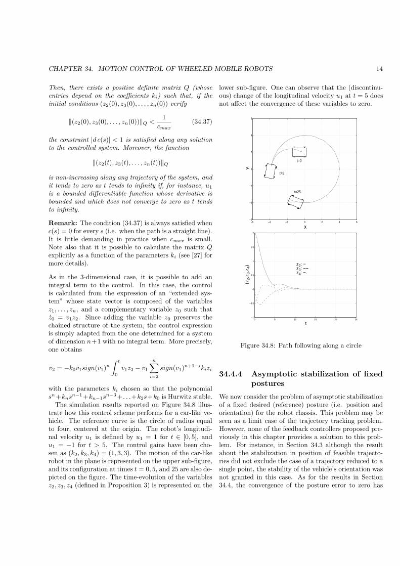
The simulation results reported on Figure 34.8 illus-trate how this control scheme performs for a car-like ve-hicle. The reference curve is the circle of radius equalto four, centered at the origin. The robot’s longitudi-nal velocity u1 is defined by u1 = 1 for t ∈ [0, 5], andu1 = −1 for t > 5. The control gains have been cho-sen as (k2, k3, k4) = (1, 3, 3). The motion of the car-likerobot in the plane is represented on the upper sub-figure,and its configuration at times t = 0, 5, and 25 are also de-picted on the figure. The time-evolution of the variablesz2, z3, z4 (defined in Proposition 3) is represented on the

lower sub-figure. One can observe that the (discontinu-ous) change of the longitudinal velocity u1 at t = 5 doesnot affect the convergence of these variables to zero.

−6 −4 −2 0 2 4 6−6

−4

−2

0

2

4

6

x

y

t=0

t=5

t=25

0 5 10 15 20 25−1

−0.5

0

0.5

1

1.5

2

t

(z 2

,z3,z

4) z2: −

z3: −− z4: −.

Figure 34.8: Path following along a circle

34.4.4 Asymptotic stabilization of fixed

postures

We now consider the problem of asymptotic stabilizationof a fixed desired (reference) posture (i.e. position andorientation) for the robot chassis. This problem may beseen as a limit case of the trajectory tracking problem.However, none of the feedback controllers proposed pre-viously in this chapter provides a solution to this prob-lem. For instance, in Section 34.3 although the resultabout the stabilization in position of feasible trajecto-ries did not exclude the case of a trajectory reduced to asingle point, the stability of the vehicle’s orientation wasnot granted in this case. As for the results in Section34.4, the convergence of the posture error to zero has


been proven when the robot’s longitudinal velocity didnot converge to zero (which excludes the case of fixedpostures).

From the automatic control point of view, the asymp-totic stabilization of fixed postures is very different fromthe problems of path following and trajectory trackingwith non-zero longitudinal velocity, much in the sameway as a human driver knows, from experience, thatparking a car at a precise location involves techniquesand skills different from those exercised when cruisingon a road. In particular, it cannot be solved by any clas-sical control method for linear systems (or based on lin-earization). Technically, the underlying general problemis the one of asymptotic stabilization of equilibria of con-trollable driftless systems with less control inputs thanstate variables. This problem has motivated numerousstudies during the last decade of the last century, frommany authors and with various angles of attack, and ithas remained a subject of active research five years later.The variety of candidate solutions proposed until now,the mathematical technicalities associated with severalof them, together with unsolved difficulties and limita-tions, particularly (but not only) in terms of robustness(an issue on which we will return), prevent us from at-tempting to cover the subject here with the ambitionof exhaustivity. Instead, we have opted for a somewhatinformal exposition of approaches which have been con-sidered, with the illustration of a few control solutions,without going into technical and mathematical details.

A central aspect of the problem, which triggered muchof the subsequent research on the control of nonholo-nomic systems, is that asymptotic stabilization of equi-libria (or fixed points) cannot be achieved by using con-tinuous feedbacks which depend on the state only (i.e.continuous pure-state feedbacks). This is a consequenceof an important result due to Brockett2 in 1983 (see alsorelated comments in Section 17.3.2).

Theorem 1 (Brockett [7]) Consider a control systemx = f(x, u) (x ∈ R

n, u ∈ Rm), with f a differentiable

function and (x, u) = (0, 0) an equilibrium of this sys-tem. A necessary condition for the existence of a contin-uous feedback control u(x) which renders the origin of theclosed-loop system x = f(x, u(x)) asymptotically stable isthe local surjectivity of the application (x, u) 7−→ f(x, u).More precisely, the image by f of any neighborhood Ω of(0, 0) in R

n+m must be a neighborhood of 0 in Rn.

2The original result by Brockett concerned differentiable feed-backs; it has later been extended to the larger set of feedbackswhich are only continuous.

This result implies that the equilibria of many control-lable (nonlinear) systems are not asymptotically stabi-lizable by continuous pure-state feedbacks. All non-holonomic WMRs belong to this category of systems.This will be shown in the case of a unicycle-type ve-hicle; the proof for the other mobile robots is similar.Let us thus consider a unicycle-type vehicle, whose kine-matic equations (34.4) can be written as x = f(x, u)with x = (x1, x2, x3), u = (u1, u2), and f(x, u) =(u1 cosx3, u1 sinx3, u2)

T , and let us show that f is notlocally onto in the neighborhood of (x, u) = (0, 0). Tothis purpose, take a vector in R

3 of the form (0, δ, 0)T . Itis obvious that the equation f(x, u) = (0, δ, 0)T does nothave a solution in the neighborhood of (x, u) = (0, 0)since the first equation, namely u1 cosx3 = 0, impliesthat u1 = 0, so that the second equation cannot have asolution if δ is different from zero.

It is also obvious that the linear approximation (aboutthe equilibrium (x, u) = (0, 0)) of the unicycle kinematicequations is not controllable. If it were, it would be pos-sible to (locally) asymptotically stabilize this equilibriumwith a linear (thus continuous) state feedback.

Therefore, by application of the above theorem, aunicycle-type mobile robot (like other nonholonomicrobots) cannot be asymptotically stabilized at a de-sired posture (position/orientation) by using a contin-uous pure-state feedback. This impossibility has moti-vated the development of other control strategies in orderto solve the problem. Three major types of controls havebeen considered:

1. continuous time-varying feedbacks, which, besidesfrom depending on the state x, depend also on theexogenous time variable (i.e. u(x, t) instead of u(x)for classical feedbacks).

2. discontinuous feedbacks, in the classical form u(x),except that the function u is not continuous at theequilibrium that one wishes to stabilize.

3. hybrid discrete/continuous feedbacks. Although thisclass of feedbacks is not defined as precisely as theother two sets of controls, it is mostly composedof time-varying feedbacks, either continuous or dis-continuous, such that the part of the control whichdepends upon the state is only updated periodically,e.g. u(t) = u(x(kT ), t) for any t ∈ [kT, (k + 1)T ),with T denoting a constant period, and k ∈ N.

We will now illustrate these approaches. In fact, onlytime-varying and hybrid feedbacks will be consideredhere. The main reason is that discontinuous feedbacks


involve difficult questions (existence of solutions, mathe-matical meaning of these solutions,...) which complicatetheir analysis and for which complete answers are notavailable. Moreover, for most of the discontinuous con-trol strategies described in the literature, the property ofstability in the sense of Lyapunov is either not grantedor remains an open issue.

Time-varying feedbacks

The use of time-varying feedbacks for the asymptoticstabilization of a fixed desired equilibrium, for a non-holonomic WMR, in order to circumvent the obstruc-tion pointed out by Brockett’s Theorem, has been firstproposed in [35]. Since then, very general results aboutthe stabilization of nonlinear systems by means of time-varying feedbacks have been obtained. For instance, ithas been proved that any controllable driftless systemcan have any of its equilibria asymptotically stabilizedwith a control of this type [11]. This includes the kine-matic models of the nonholonomic mobile robots hereconsidered. We will illustrate this approach in the caseof unicycle-type and car-like mobile robots modeled bythree and four-dimensional chained systems respectively.In order to consider the three-dimensional case, let uscome back on the results obtained in Section 34.4.3 forpath following. We have established (see Proposition 6)that the control v2 = −v1k2z2 − |v1|k3z3 applied to thesystem

z1 = v1z2 = v1z3z3 = v2

renders the function V (z) defined by (34.33) non-increasing along any trajectory of the controlled system,i.e.

V = −k3k2|v1|z

23

and ensures the convergence of z2 and z3 to zero if, forinstance, v1 does not tend to zero as t tends to infinity.For example, if v1(t) = sin t, the proposition applies, z2and z3 tend to zero, and

z1(t) = z1(0) +∫ t

0v1(s) ds = z1(0) +

∫ t

0sin s ds

= z1(0) + 1− cos t

so that z1(t) oscillates around the mean value z1(0) + 1.To reduce these oscillations, one can multiply v1 by afactor which depends on the current state. Take, forexample, v1(z, t) = ‖(z2, z3)‖ sin t, that we complementwith a stabilizing term like −k1z1 with k1 > 0, i.e.

v1(z, t) = −k1z1 + ‖(z2, z3)‖ sin t .

The feedback control so obtained is time-varying andasymptotically stabilizing.

Proposition 9 [37] The continuous time-varying feed-back

v1(z, t) = −k1z1 + α‖(z2, z3)‖ sin tv2(z, t) = −v1(z, t)k2z2 − |v1(z, t)|k3z3

(34.38)

with α, k1,2,3 > 0, renders the origin of the 3-dimensionalchained system globally asymptotically stable.

The above proposition can be extended to chained sys-tems of arbitrary dimension [37]. For the case n = 4,which corresponds to the car-like robot, one has the fol-lowing result.

Proposition 10 [37] The continuous time-varying feed-back

v1(z, t) = −k1z1 + α‖(z2, z3, z4)‖ sin tv2(z, t) = −|v1(z, t)|k2z2 − v1(z, t)k3z3

−|v1(z, t)|k4z4

(34.39)

with α, k1,2,3,4 > 0 chosen such that the polynomial s3 +k4s

2 + k3s + k2 is Hurwitz-stable, renders the origin ofthe 4-dimensional chained system globally asymptoticallystable.

Figure 34.9 below illustrates the previous result. Forthis simulation, the parameters α, k1,2,3,4 in the feedbacklaw (34.39) have been chosen as α = 3 and k1,2,3,4 =(1.2, 10, 18, 17). The upper sub-figure shows the motionof the car-like robot in the plane. The initial configura-tion, at time t = 0, is depicted in plain lines, whereas thedesired configuration is shown in dashed lines. The time-evolution of the variables x, y, and θ (i.e. position andorientation variables corresponding to the model (34.5))is shown on the lower sub-figure.

A shortcoming of this type of control, very clear onthis simulation, is that the system’s state converges tozero quite slowly. One can show that the rate of conver-gence is only polynomial, i.e. it is commensurable witht−α (for some α ∈ (0, 1)) for most of the trajectories ofthe controlled system. This slow rate of convergence isrelated to the fact that the control function is Lipschitz-continuous with respect to x. It is a characteristics ofsystems the linear approximation of which is not stabi-lizable, as specified in the following proposition.

Proposition 11 Consider the control system x =f(x, u) (x ∈ R

n, u ∈ Rm) with f being differentiable,


−1 −0.5 0 0.5 1 1.5 2 2.5−1

−0.5

0

0.5

1

1.5

2

2.5

x

y

0 10 20 30 40 50 60 70 80−1

−0.5

0

0.5

1

1.5

2

t

(x,

y,θ)

x: − y: −− θ: −.

Figure 34.9: Stabilization with a Lipschitz-continuouscontroller

and (x, u) = (0, 0) an equilibrium point of this sys-tem. Assume that the linear approximation of this sys-tem is not stabilizable. Consider also a continuous time-varying feedback u(x, t), periodic with respect to t, suchthat u(0, t) = 0 for any t, and such that u(., t) is k(t)-Lipschitz continuous with respect to x, for some boundedfunction k. This feedback cannot yield uniform exponen-tial convergence to zero of the closed-loop systems solu-tions: there does not exist constants K > 0 and γ > 0such that, along any trajectory x(.) of the controlled sys-tem, one has

|x(t)| ≤ K|x(t0)|e−γ(t−t0) (34.40)

The intuitive reason behind this impossibility can eas-ily be illustrated on the unicycle example. When us-ing the chain form representation, the second equation isz2 = v1z3. Since the linearization, around (z = 0, v = 0)of this equation gives z2 = 0, the linear approximation ofthe system is not controllable (nor stabilizable). In theseconditions, exponential convergence, when applying alinear feedback, would necessitate the use of gains grow-

ing to infinity, thus ruling out the property of Lipschitz-continuity. This type of reasoning, coupled to the needof better performance and efficiency, has triggered thedevelopment of stabilizing time-varying feedbacks whichare continuous, but not Lipschitz-continuous. Examplesof such feedbacks, yielding uniform exponential conver-gence, are given in the following propositions for chainedsystems of dimension three and four respectively.

Proposition 12 [27] Let α, k1,2,3 > 0 denote scalarssuch that the polynomial p(s) = s2+k3s+k2 is Hurwitz-stable. For any integers p, q ∈ N

∗, let ρp,q denote thefunction defined on R

2 by

∀z2 = (z2, z3) ∈ R2, ρp,q(z2) =

(

|z2|p

q+1 + |z3|pq

)1p

Then, there exists q0 > 1 such that, for any q ≥ q0 andp > q + 2, the continuous state feedback

v1(z, t) = −k1(z1 sin t− |z1|) sin t+ αρp,q(z2) sin t

v2(z, t) = −v1(z, t)k2z2

ρ2p,q(z2)− |v1(z, t)|k3

z3ρp,q(z2)

(34.41)renders the origin of the 3-dimensional chained systemglobally asymptotically stable, with a uniform exponentialrate of convergence.

The parenthood of the controls (34.38) and (34.41) isnoticeable. One can also verify that the control (34.41)is well defined (by continuity) at z2 = 0. More precisely,the ratios

z2ρ2p,q(z2)

andz3

ρp,q(z2)

which are obviously well defined when z2 6= 0, tend tozero when z2 tends to zero. This guarantees the conti-nuity of the control law.

The property of exponential convergence pointed outin the above result calls for some remarks. Indeed, thisproperty does not exactly correspond to the classical ex-ponential convergence property associated with stablelinear systems. In this latter case, exponential conver-gence implies that the relation (34.40) is satisfied. Thiscorresponds to the common notion of “exponential sta-bility”. In the present case, this inequality becomes

ρ(z(t)) ≤ Kρ(z(t0))e−γ(t−t0)

for some function ρ, defined for example by ρ(z) =|z1| + ρp,q(z2, z3), with ρp,q as specified in Proposition12. Although the function ρ shares common features


with the Euclidean norm of the state vector (it is defi-nite positive and it tends to infinity when ‖z‖ tends toinfinity), it is not equivalent to this norm. Of course,this does not change the fact that each component zi ofz converges to zero exponentially. However, the transientbehavior is different because one only has

|zi(t)| ≤ K‖z(t0)‖αe−γ(t−t0)

with α < 1, instead of

|zi(t)| ≤ K‖z(t0)‖e−γ(t−t0)

In the case of the four-dimensional chained system,one can establish the following result, which is similar toProposition 12.

Proposition 13 [27] Let α, k1, k2, k3, k4 > 0 be chosensuch that the polynomial p(s) = s3 + k4s

2 + k3s + k2is Hurwitz-stable. For any integers p, q ∈ N

∗, let ρp,qdenote the function defined on R

3 by

ρp,q(z2) =(

|z2|p

q+2 + |z3|p

q+1 + |z4|pq

)1p

with z2 = (z2, z3, z4) ∈ R3. Then, there exists q0 > 1

such that, for any q ≥ q0 and p > q + 2, the continuousstate feedback

v1(z, t) = −k1(z1 sin t− |z1|) sin t+ αρp,q(z2) sin t

v2(z, t) = −|v1(z, t)|k2z2

ρ3p,q(z2)− v1(z, t)k3

z3ρ2p,q(z2)

−|v1(z, t)|k4z4

ρp,q(z2)

(34.42)renders the origin of the 4-dimensional chained systemglobally asymptotically stable, with a uniform exponentialrate of convergence.

The performance of the control law (34.42) is illus-trated by the simulation results shown in Figure 34.10.The control parameters have been chosen as follows:α = 0.6, k1,2,3,4 = (1.6, 10, 18, 17), q = 2, p = 5. Thecomparison with the simulation results of Figure 34.9shows a clear gain in performance.

Hybrid feedbacks

These feedbacks constitute an alternative for the asymp-totic stabilization of fixed postures. They may be seenas a mixt of open-loop and feedback controls in the sensethat the dependence on the state is, in general, only up-dated periodically (by contrast with time-varying feed-backs which are updated continuously). Between two

−1 −0.5 0 0.5 1 1.5 2 2.5−1

−0.5

0

0.5

1

1.5

2

2.5

x

y

0 10 20 30 40 50 60 70 80−1

−0.5

0

0.5

1

1.5

2

t

(x,

y,θ)

x: − y: −− θ: −.

Figure 34.10: Stabilization with a continuous (non-Lipschitz) time-varying feedback

updates, the control works in open-loop. Nonetheless,this type of control may present some advantages withrespect to time-varying feedbacks. This point is brieflycommented upon a little further. An example of a hybridfeedback is provided in the following proposition.

Proposition 14 [26] The hybrid feedback law v definedby

v(t) = v(z(kT ), t) ∀t ∈ [kT, (k + 1)T ) (34.43)

with

v1(z, t) =1T [(k1 − 1)z1 + 2πρ(z) sin(ωt)]

v2(z, t) =1T [(k3 − 1)z3 + 2(k2 − 1) z2

ρ(z) cos(ωt)]

and

k1,2,3 ∈ (−1, 1), ω =2π

T, ρ(z) = α2|z2|

1/2 (α2 > 0)

is a K(T )-exponential stabilizer for the 3-d chained sys-tem.


The property of “K(T )-exponential stabilizer” evoked inthe above proposition means that there exist positiveconstants K, η, and γ, with γ < 1, such that for any z0,the solution at time t of the controlled system associatedwith the initial condition z0 at time t = 0, which wedenote as z(t, 0, z0), satisfies for any k ∈ N and any s ∈[0, T ) the following inequalities:

‖z((k + 1)T, 0, z0)‖ ≤ γ‖z(kT, 0, z0)‖

and‖z(kT + s, 0, z0)‖ ≤ K‖z(kT, 0, z0)‖

η

These relations imply the exponential convergence of thesystem’s trajectories to the origin z = 0. They do notimply the stability of this point because ‖z(t, 0, z0)‖ mayvanish at some time t = t and not remain equal tozero everafter. Note, however, that if ‖z(kT, 0, z0)‖ = 0for some k ∈ N, then the above relations imply that‖z(t, 0, z0)‖ = 0 for all t ≥ kT .

In the case of four-dimensional systems, a result simi-lar to Proposition 14 can also be established.

Proposition 15 [26] The hybrid feedback law v definedby

v(t) = v(z(kT ), t) ∀t ∈ [kT, (k + 1)T ) (34.44)

with

v1(z, t) =1T [(k1 − 1)z1 + 2πρ(z) sin(ωt)]

v2(z, t) =1T [(k4 − 1)z4 + 2(k3 − 1) z3

ρ(z) cos(ωt)

+8(k2 − 1) z2ρ2(z) cos(2ωt)]

k1,2,3,4 ∈ (−1, 1), ω = 2πT , and ρ(z) = α2|z2|

1/4 +

α3|z3|1/3 (α2,3 > 0), is a K(T )-exponential stabilizer for

the 4-d chained system.

The simulation results reported in Figure 34.11 il-lustrate the application of the feedback law (34.44).The control parameters have been chosen as T = 3,k1,2,3,4 = 0.25, and α2,3 = 0.95. The control perfor-mance is similar to the one observed in Figure 34.10, ascould be expected from the fact that both controls yieldexponential convergence to the origin.

34.4.5 Limitations inherent to the con-

trol of nonholonomic systems

Let us first mention some problems associated with thenonlinear time-varying and hybrid feedbacks just pre-sented. An ever important issue, when studying feed-back control, is robustness. Indeed, if it were not for

−1 −0.5 0 0.5 1 1.5 2 2.5−1

−0.5

0

0.5

1

1.5

2

2.5

x

y

0 10 20 30 40 50 60 70 80−1

−0.5

0

0.5

1

1.5

2

t

(x,

y,θ)

x: − y: −− θ: −.

Figure 34.11: Stabilization with a hybrid dis-crete/continuous controller

the sake of robustness, feedback control would loosemuch of its value and interest with respect to open-loop control solutions. Robustness aspects are multi-ple also. One of them concerns the sensitivity to mod-eling errors. For instance, in the case of a unicycle-type robot whose kinematic equations are in the formx = u1b1(x) + u2b2(x), one would like to know whethera feedback law which stabilizes an equilibrium of thissystem also stabilizes this equilibrium for the “neigh-bor” system x = u1(b1(x)+ εg1(x))+u2(b2(x)+ εg2(x)),with g1 and g2 denoting continuous applications, and εa parameter which quantifies the modeling error. Thistype of error can account, for example, for a small uncer-tainty concerning the orientation of the actuated wheelsaxle with respect to the chassis, which results in a biasin the measurement of this orientation. One can showthat time-varying control laws like (34.41) are not robustwith respect to this type of error in the sense that, forcertain functions g1 and g2, and for ε arbitrarily small,the system’s solutions end up oscillating in the neighbor-hood of the origin, instead of converging to the origin.


In other words, both the properties of stability of theorigin and of convergence to this point can be jeopar-dized by arbitrarily small modeling errors, even in theabsence of measurement noise. In this respect, the hy-brid control law (34.43) is more robust: the exponen-tial convergence to the origin of the controlled system’ssolutions is still obtained when ε is small enough. How-ever, the slightest discretization uncertainty can producethe same type of local instability. In view of the above-mentioned problems, one is brought to question the ex-istence of fast (exponential) stabilizers endowed with ro-bustness properties similar to those of stabilizing linearfeedbacks for linear systems. The answer is that, to ourknowledge, no such control solution (either continuousor discontinuous) has ever been found. More than likelysuch a solution does not exist for nonholonomic systems.Robustness of the stability property against modelingerrors, and control discretization and delays, has beenproved in some cases, but this could only be achievedwith Lipschitz-continuous feedbacks which, as we haveseen, yield slow convergence. The classical compromisebetween robustness and performance thus seems muchmore acute than in the case of stabilizable linear sys-tems (or nonlinear systems whose linear approximationis stabilizable).

A second issue is the proven non-existence of a “uni-versal” feedback controller capable of stabilizing any fea-sible reference state-trajectory asymptotically [20]. Thisis another notable difference with the linear case. In-deed, given a controllable linear system x = Ax + Bu,the feedback controller u = ur + K(x − xr), with K again matrix such that A + BK is Hurwitz stable, ex-ponentially stabilizes any feasible reference trajectory xr(solution to the system) associated with the control inputur. The non-existence of such a controller, in the case ofnonholonomic mobile robots, is related to the conditionsupon the longitudinal velocity stated in previous propo-sitions concerning trajectory stabilization (Propositions4 and 5). It basically indicates that such conditions can-not be removed entirely: whatever the chosen feedbackcontroller, there always exists a feasible reference trajec-tory that this feedback cannot asymptotically stabilize.Note that this limitation persists when considering non-standard feedbacks (like e.g. time-varying periodic feed-backs capable of asymptotically stabilizing reference tra-jectories which are reduced to a single point). Moreover,it has clear practical consequences because there are ap-plications (automatic tracking of a human driven car, forinstance) for which the reference trajectory, and thus itsproperties, are not known in advance (is the leading car

going to keep moving or stop?) so that one cannot eas-ily decide on which controller to use. Switching betweenvarious controllers is a possible strategy, which has beenstudied by some authors and may give satisfactory re-sults in many situations. However, since implementinga pre-defined switching strategy between two controllerssums up to designing a third controller, this does notsolve the core of the problem nor grant any certitude ofsuccess.

A third issue, which is not specific to nonholonomicsystems, but has seldom been addressed in the nonlinearcontrol literature, concerns the problem of tracking non-feasible trajectories (i.e. trajectories which are not so-lutions to the system’s equations). Since exact trackingis not possible, by definition of a non-feasible trajectory,the control objective is then to ensure that the trackingerrors shrink to, and everafter never exceed, certain non-zero thresholds. The fact that these thresholds can theo-retically be arbitrarily small in the case of nonholonomicsystems, if the amplitude of the velocity control inputs isnot limited, makes this problem particularly relevant forthese systems. This can be termed as a practical stabi-lization objective which, although slightly less ambitiousthan the objective of asymptotic stabilization consideredin previous sections, opens up both the control designproblem and the range of applications significantly. Forinstance, it allows to address the problem of tracking anomnidirectional vehicle with a unicycle-type, or a car-like, vehicle. In the context of planning a trajectory withobstacle avoidance, transforming a non-feasible trajec-tory into a feasible approximation for a certain mobilerobot can be performed by applying a practical stabi-lizer to a model of this robot and by numerical integra-tion of the system’s closed-loop equations. Also, if onere-formulates the former question about the existenceof a “universal” stabilizer, with the objective of asymp-totic stabilization now replaced by the one of practicalstabilization, then the answer becomes positive: such astabilizer exists and, moreover, the reference trajectoriesdo not even have to be feasible.

34.4.6 Practical stabilization of arbi-

trary trajectories based on the

transverse function approach

A possible approach for the design of practical stabilizersin the case of controllable driftless is described in [29].Some of its basic principles, here adapted to the specificexamples of unicycle-type and car-like mobile robots, arerecalled next.


Let us introduce some matrix notation that will beused in this section.

R(θ) =

(

cos θ − sin θsin θ cos θ

)

, S =

(

0 −11 0

)

R(θ) =

(

R(θ) 00 1

)

Unicycle case: With the above notation, the kinematicmodel (34.4) can be written as

g = R(θ)Cu (34.45)

with g = (x, y, θ)′ and

C =

1 00 00 1

Let us now consider a smooth function

f : α 7−→ f(α) =

fx(α)fy(α)fθ(α)

with α ∈ S1 = R/2πZ (i.e. α is an angle variable), anddefine

g :=

xyθ

:= g − R(θ − fθ(α))f(α)

=

(

xy

)

−R(θ − fθ(α))

(

fx(α)fy(α)

)

θ − fθ(α)

(34.46)

Note that g can be viewed as the situation3 of a frameFm(α) the origin of which has components

−R(−fθ(α))

(

fx(α)fy(α)

)

in the frame Fm. Hence, Fm(α) is all the more closeto Fm as the components of f(α) are small. For anysmooth time function t 7−→ α(t), and along any solutionto system (34.45), the time-derivative of g is given by

˙g = R(θ)u (34.47)

with

u = A(α)(

R(fθ(α)) − ∂f∂α (α)

)

(

Cuα

)

(34.48)

3In term of differential geometry, g is the product of g by theinverse f(α)−1 of f(α), in the sense of the Lie group operations inSE(2).

and

A(α) =

I2 −S

(

fx(α)fy(α)

)

0 1

(34.49)

From (34.47) and (34.48), one can view α as a comple-mentary control input which can be used to monitor themotion of the frame Fm(α). More precisely, Fm(α) canbe viewed as an omnidirectional frame provided that ucan be rendered equal to any vector of R

3, i.e. providedthat the mapping (u, α) 7−→ u is onto. Let us determinewhen this condition is satisfied. Equation (34.48) canalso be written as

u = A(α)H(α)

(

uα

)

(34.50)

with

H(α) =

cos fθ(α) 0 −∂fx∂α (α)

sin fθ(α) 0 −∂fy∂α (α)

0 1 −∂fθ∂α (α)

(34.51)

Since A(α) is invertible, Fm(α) is omnidirectional if andonly if the matrix H(α) is also invertible. A function fwhich satisfies this property for any α ∈ S1 is called a“transverse function” [28]. The issue of the existence ofsuch functions has been treated in the much more generalcontext of the transverse function approach [28, 29]. Inthe present case, a family of transverse functions is givenby:

f(α) =

ε sinαε2η sin 2α4

arctan(εη cosα)

with ε, η > 0 (34.52)

Indeed, one can verify that for any α ∈ S1, detH(α) =

− ε2η2 cos(arctan(εη cosα)) < 0. Note that the compo-

nents of f uniformly tend to zero as ε tends to zero, sothat the associated omnidirectional frame Fm(α) can bemade arbitrarily close to Fm by choosing ε small (butdifferent from zero).

Now, let t 7−→ gr(t) = (xr(t), yr(t), θr(t))T denote a

smooth, but otherwise arbitrary, reference trajectory. Itis not difficult to derive from (34.47) a feedback law uwhich asymptotically stabilizes g at gr. A possible choiceis given for example by

u = R(−θ)(gr − k(g − gr)) (34.53)

which implies that ( ˙g− gr) = −k(g− gr) and, therefore,that g − gr = 0 is an exponentially stable equilibrium of


the above equation for any k > 0. Then, it follows from(34.46) that

limt→+∞

(

g(t)− gr(t)− R(θr(t))f(α(t)))

= 0 (34.54)

The norm of the tracking error ‖g−gr‖ is thus ultimatelybounded by the norm of f(α) which, in view of (34.52),can be made arbitrarily small via the choice of ε. It isin this sense that practical stabilization is achieved. Thecontrol u for the unicycle-like robot is then calculated byinverting the relation (34.50) and using the expression(34.53) of u.

While it can be tempting to use very small values ofε for the transverse function f in order to obtain a goodtracking precision, one must be aware of the limits ofthis strategy. Indeed, when ε tends to zero, the matrixH(α) defined by (34.51) becomes ill-conditioned, and itsdeterminant tends to zero. This implies, by (34.50), thatthe robot’s velocities u1 and u2 may become very large.In particular, when the reference trajectory gr is not fea-sible, many manoeuvres are likely to occur. Note thatthis difficulty is intrinsic to the robot’s nonholonomy andthat it cannot be circumvented (think about the prob-lem of parking a car in a very narrow parking place). Forthis reason, trying to impose a very accurate tracking ofnon-feasible trajectories is not necessarily a good optionin practice. On the other hand, when the trajectory isfeasible, manoeuvres are not needed to achieve accuratetracking, so that smaller values of ε can be used in thiscase. This clearly leads to a dilemma when the refer-ence trajectory is not known in advance and its proper-ties in term of feasibility can vary with time. A controlstrategy which addresses this issue, based on the use oftransverse functions whose magnitude can be adaptedonline, is proposed in [3]. Experimental validations ofthe present approach on a unicycle-like robot can alsobe found in [2].

Car case: The control approach presented above can beextended to car-like vehicles (and also to the trailer case).Again, the idea is to associate with the robot’s frame Fman omnidirectional “companion”frame Fm(α) which canbe maintained arbitrarily close to Fm via the choice ofsome design parameters. Let us show how this can bedone for a car-like vehicle. To simplify the forthcomingequations, let us rewrite System (34.5) as


θ = u1ξ

ξ = uξ

with ξ = (tanφ)/L and uξ = u2(1 + tan2 φ)/L. Thissystem can also be written as (compare with (34.45))

g = R(θ)C(ξ)u1ξ = uξ

(34.55)

with g = (x, y, θ)T and C(ξ) = (1, 0, ξ)T . Let us nowconsider a smooth function

f : α 7−→ f(α) =

(

fg(α)fξ(α)

)

=

fx(α)fy(α)fθ(α)fξ(α)

with α ∈ S1×S1 (i.e. α = (α1, α2)), and define (comparewith (34.46))

g :=

xyθ

:= g − R(θ − fθ(α))fg(α)

=

(

xy

)

−R(θ − fθ(α))

(

fx(α)fy(α)

)

θ − fθ(α)

(34.56)

which, as in the unicycle case, can be viewed as the sit-uation of some “companion” frame Fm(α). By differen-tiating g along any smooth time function t 7−→ α(t) andany solution to system (34.55), one can verify that Eq.(34.47) is still satisfied, except that u is now given by

u = A(α)(

R(fθ(α)) −∂fg∂α1

(α) −∂fg∂α2

(α))

C(ξ)u1α1α2

(34.57)rather than by (34.48) (with A(α) still defined by(34.49)). Using the fact that

C(ξ)u1 = C(fξ(α))u1 + (C(ξ)− C(fξ(α)))u1

=

10

fξ(α)

u1 +

00

ξ − fξ(α)

u1

the equation (34.57) can also be written as

u = A(α)H(α)

u1α1α2

+A(α)

00

u1(ξ − fξ(α))

(34.58)

with

H(α) =

cos fθ(α) − ∂fx∂α1

(α) − ∂fx∂α2

(α)

sin fθ(α) −∂fy∂α1

(α) −∂fy∂α2

(α)

fξ(α) − ∂fθ∂α1

(α) − ∂fθ∂α2

(α)

(34.59)


By settinguξ = fξ(α)− k(ξ − fξ(α) (34.60)

with k > 0, it follows from (34.55) that ξ − fξ(α) ex-ponentially converges to zero. Hence, after some tran-sient phase whose duration is commensurable with 1/k,ξ − fξ(α) ≈ 0, and (34.58) reduces to

u = A(α)H(α)

u1α1α2

(34.61)

Provided that the function f is such that H(α) is al-ways invertible, this latter relation means that the frameFm(α) associated with g is omnidirectional. Any func-tion f for which this property is satisfied is called a trans-verse function. Once it has been determined, one canproceed as in the unicycle case to asymptotically stabi-lize an arbitrary reference trajectory gr for g, for exampleby defining u as in (34.53). The control u1 for the car isthen obtained by inverting relation (34.61). The follow-ing lemma specifies a family of transverse functions forthe car case.

Lemma 1 [30] For any ε > 0 and any η1, η2, η3 suchthat η1, η2, η3 > 0 and 6η2η3 > 8η3 + η1η2, the functionf defined by

f(α) =

f1(α)f4(α)

arctan(f3(α))f2(α) cos

3 f3(α)

with f : S1 × S1 −→ R4 given by f(α) =

ε(sinα1 + η2 sinα2)εη1 cosα1

ε2(η1 sin 2α1

4 − η3 cosα2)

ε3(η1sin2 α1 cosα1

6 − η2η3 sin 2α2

4 − η3 sinα1 cosα2)

satisfies the transversality condition detH(α) 6= 0 ∀α,with H(α) defined by (34.59).

The simulation results reported in Figure 34.12 illus-trate the application of this control approach for a car-like robot. The reference trajectory is defined by theinitial condition gr(0) = 0 and its time-derivative

gr(t) =

(0, 0, 0)T if t ∈ [0, 30](1, 0, 0)T if t ∈ [30, 38](0, 0.3, 0)T if t ∈ [38, 53](−1, 0, 0)T if t ∈ [53, 61](0, 0, 0.2)T if t ∈ [61, 80]

This corresponds to a fixed situation when t ∈ [0, 30],three sequences of pure translational motion when t ∈[30, 61], and a pure rotational motion when t ∈ [61, 80].Let us remark that this trajectory is not feasible for thecar-like robot when t ∈ [38, 53], since it corresponds to alateral translation in the direction of the unit vector ~rof the frame Fr associated with gr, nor when t ∈ [61, 80],since a rear-drive car cannot perform pure rotational mo-tion. The initial configuration of the car-like robot, att = 0, is g(0) = (0, 1.5, 0), and the initial steering wheelangle is φ(0) = 0.

−2 0 2 4 6 8 10−2

−1

0

1

2

3

4

5

6

x

y

t=0

t=20 t=34

t=45

t=57 t=80

0 10 20 30 40 50 60 70 80−1

−0.5

0

0.5

1

1.5

t

(x,y

,θ)

x: − y: −− θ: −.

Figure 34.12: Practical stabilization of an arbitrary tra-jectory by the t.f. approach

On the upper sub-figure, the robot is drawn in plainline at several time-instants, whereas the chassis of thereference vehicle is drawn in dashed-line at the sametime-instants. The figure also shows the trajectory ofthe point located at mid-distance of the robot’s rear


wheels. The lower sub-figure shows the time evolutionof the tracking error expressed in the reference frame(i.e. (xe, ye) as defined by (34.20), and θe = θ − θr). Itfollows from (34.54) that after the transient phase asso-ciated with the exponential convergence of g to zero, theultimate bound for |xe|, |ye|, and |θe| is upper-boundedby the maximum amplitude of the functions fx, fy, andfθ respectively. For this simulation, the control parame-ters of the transverse function f of Lemma 1 have beenchosen as follows: ε = 0.17, η1,2,3 = (12, 2, 20). Withthese values, one can verify that |fx|, |fy|, and |fθ| arebounded by 0.51, 0.11, and 0.6 respectively. This is con-sistent with the time-evolution of the tracking error onthe figure. As pointed out for the unicycle case, a highertracking precision could be obtained by decreasing thevalue of ε, but this would involve larger values of thecontrol inputs and also more frequent manoeuvres, espe-cially on the time intervals [38, 53] and [61, 80] when thereference trajectory is not feasible.

34.5 Complementary issues and

bibliographical guide

General trailer systems:Most of the control design approaches here presentedand illustrated for unicycle and car-like vehicles canbe extended to the case of trains of vehicles composedof trailers hitched to a leading vehicle. In particular,the methods of Section 34.4 which are specific tononholonomic systems can be extended to this case,provided that the kinematic equations of motion ofthe system can be transformed (at least semi-globally)into a chained system [37]. This basically requires thatthe hitch point of each trailer is located on the rearwheels axle of the preceding vehicle [38]. For instance,the transformation to the chained form is not possiblewhen there are two (or more) successive trailers withoff-axle hitch points [34]. So-called “general trailersystems” (with off-axle hitch points) raise difficultcontrol design issues, and the literature devoted tothem is sparse. For this reason, and also because thesesystems are not met in applications as frequently assimpler vehicles, control methods specifically developedfor them are not reported here. Nonetheless, a fewrelated references are given next. The path followingproblem has been considered in e.g. [6] for a systemwith two trailers and, more generally, in [19, Ch. 3]and [1] for an arbitrary number of trailers. To ourknowledge, the problem of stabilizing non-stationary

reference trajectories has not been addressed for thesesystems (except in the single trailer case for whichthe system can be transformed into the chained form[17, 34]). As a matter of fact, the explicit calculationof feasible trajectories joining a given configuration toanother is already a very difficult problem, even in theabsence of obstacles. As for the asymptotic stabilizationof fixed configurations, the problem can (in theory)be solved by using existing general methods developedfor the larger class of controllable driftless systems.However, the calculations associated with these methodsquickly become intractable when the number of trailersincreases. More specific and simpler ones have beenproposed in [21], for an arbitrary number of trailersand the asymptotic stabilization of a reduced set ofconfigurations, and in [42], in the case of two trailersand arbitrary fixed configurations.

Sensor-based motion control:The control laws described in the present chapter,and their calculation, involve the on-line measurement,eventually complemented by the on-line estimation, ofvariables depending on the position of the vehicles intheir environment. Measures can be acquired via theuse of various sensors (odometry, GPS, proximetry, vi-sion,...). Usually, various treatments are applied to rawsensory data prior to computing the control variablesthemselves. For instance, noise-filtering and state-estimation are such basic operations, well documentedin the Automatic control literature. Among all sensors,vision sensors play a particularly important role inrobotic applications, due to the richness and versatilityof the information which they provide. The combinationof visual data with feedback control is often referredto as visual servoing. In Chapter 24, a certain numberof visual servoing tasks are addressed, mostly in thecontext of manipulation and/or under the assumptionthat realizing the robot task is equivalent to controllingthe pose of a camera mounted on an omnidirectionalmanipulator. In a certain number of cases, the conceptsand methods described in this chapter can be adapted,without much effort, to the context of mobile robots.These cases basically correspond to the control methodsadapted from robotic manipulation which are describedin Section 34.3 of the present chapter. For instance, au-tomatic driving via the control of the visually estimatedlateral distance between a robotic vehicle and the side ofa road, or car-platooning by controlling the frontal andlateral distances to a leading vehicle, can be addressedwith the control techniques reported in Chapter 24.


The reason is that it is possible to simply recast thesetechniques in the form of the control laws proposedin Section 34.3. However, there are also vision-basedapplications for nonholonomic mobile robots whichcannot be solved by applying classical visual-servoingtechniques. This is the case, for instance, of the taskobjectives addressed in Section 34.4, an example ofwhich is the stabilization of the complete posture (i.eposition and orientation) of a nonhonomic vehicle at adesired one. Vision-based-control problems of this typehave been addressed in [3, 23].

A few former surveys on the control of WMRs havebeen published. Let us mention [9, 18], and [43], whichcontain chapters on the modeling and control issues. Adetailed classification of kinematic and dynamic mod-els for the different types of WMR structures, on whichChapter 17 is based, is provided in [8]. The use of thechain form to represent WMR equations has been pro-posed in [31], then generalized in [39].

Path following may have been the first mobile robotcontrol problem addressed by researchers in Robotics.Among the pioneering works, let us cite [14, 32]. Severalresults presented in the present chapter are based on [36,37].

The problem of tracking admissible trajectories forunicycle-type and car-like vehicles is treated in the books[9, 18, 43], and also in numerous conference and journalpapers. Several authors have addressed this problem byapplying dynamic feedback linearization techniques. Inthis respect, one can consult [12, 13, 15], and [9, Chap.8], for instance.

Numerous papers on the asymptotic stabilization offixed configurations have been published. Among them,[16] provides an early overview of feedback control tech-niques elaborated for this purpose, and also a list of ref-erences. The first result presenting a time-varying feed-back solution to this problem, in the case of a unicycle-type vehicle, is in [35]. The conference paper [25] pro-vides a survey on time-varying feedback stabilization, inthe more general context of nonlinear control systems.More specific results, like Propositions 9 and 12, aregiven in [27, 37]. Other early results on the design ofsmooth time-varying feedbacks can be found in [33, 41],for example. Concerning continuous (but not Lipschitz-continuous) time-varying feedbacks yielding exponentialconvergence, one can consult [24]. Designs of hybrid dis-crete/continuous fixed-point stabilizers can be found in[5, 22, 40], for instance. The control law in Proposition14 is taken from [26]. Discontinuous control design tech-

niques are not addressed in the present chapter, but theinterested reader will find examples of such feedbacks in[4, 10].

To our knowledge, the control approach presented inSection 34.4.6, which is based on the concept of trans-verse functions [28, 29], is the first attempt to addressthe problem of tracking “arbitrary” trajectories (i.e. notnecessarily feasible for the controlled robot). Implemen-tation issues and experimental results for this approachcan be found in [2, 3]. An overview of trajectory trackingproblems for wheeled mobile robots, with a detailed casestudy of car-like systems, is presented in [30].

Bibliography

[1] C. Altafini, “Path following with reduced off-tracking formultibody wheeled vehicles,” IEEE Trans. on ControlSystems Technology, pp. 598–605, vol. 11, 2003.

[2] G. Artus, P. Morin and C. Samson, “Tracking of an om-nidirectional target with a nonholonomic mobile robot,”in Proc. of IEEE Conf. on Advanced Robotics (ICAR),pp. 1468–1473, 2003.

[3] G. Artus, P. Morin and C. Samson, “Control of a maneu-vering mobile robot by transverse functions,” in Proc.of Symp. on Advances in Robot Kinematics (ARK),pp. 459–468, 2004.

[4] A. Astolfi, “Discontinuous control of nonholonomic sys-tems,” Systems & Control Letters, vol. 27, pp. 37–45,1996.

[5] M. K. Bennani and P. Rouchon, “Robust stabilization offlat and chained systems,” in Proc. of European ControlConference, pp. 2642–2646, 1995.

[6] P. Bolzern, R.M. DeSantis, A. Locatelli and D. Mascioc-chi, “Path-tracking for articulated vehicles with off-axlehitching,” IEEE Trans. on Control Systems Technology,vol. 6, pp. 515–523, 1998.

[7] R.W. Brockett, “Asymptotic stability and feedback sta-bilization,” Differential Geometric Control Theory, edi-tors R.W. Brockett, R.S. Millman and H.J. Sussmann,Birkauser, 1983.

[8] G. Campion, G. Bastin and B. d’Andrea-Novel, “Struc-tural properties and classification of kynematic and dy-namic models of wheeled mobile robots,” IEEE Trans.on Robotics and Automation, vol. 12, pp. 47–62, 1996.

[9] C. Canudas de Wit, B. Siciliano and G. Bastin, “Theoryof robot control,” Springer Verlag, 1996.

[10] C. Canudas de Wit and O. J. Sørdalen, “Exponentialstabilization of mobile robots with nonholonomic con-straints,” IEEE Trans. on Automatic Control, vol. 37,no. 11, pp. 1791–1797, 1992.

[11] J.-M. Coron, “Global asymptotic stabilization for con-trollable systems without drift,” Mathematics of Con-trol, Signals, and Systems, vol. 5, pp. 295–312, 1992.

[12] B. d’Andrea-Novel, G. Campion and G. Bastin,“Control of nonholonomic wheeled mobile robots bystate feedback linearization,” International Journal ofRobotics Research, vol. 14, pp. 543–559, 1995.

[13] A. De Luca and M.D. Di Benedetto, “Control of non-holonomic systems via dynamic compensation,” Kyber-netica, vol. 29, pp. 593–608, 1993.

[14] E.D. Dickmanns and A. Zapp, “Autonomous high speedroad vehicle guidance by computer vision,” in Proc. ofIFAC World Congress, 1987.

[15] M. Fliess, J. Levine, P. Martin and P. Rouchon, “Flat-ness and defect of non-linear systems: introductory the-ory and examples,” Int. J. of Control, vol. 61, pp. 1327–1361, 1995.

[16] I. Kolmanovsky and N.H. McClamroch, “Developmentsin nonholonomic control problems,” IEEE Control Sys-tems, pp.20–36, 1995.

[17] F. Lamiraux and J.-P. Laumond, “A practical approachto feedback control for a mobile robot with trailer,” inProc. of IEEE Int. Conf. on Robotics and Automation,pp. 3291–3296, 1998.

[18] “Robot Motion Planning and Control,” Lecture Notesin Control and Information Sciences, Springer Verlag,editor J.-P. Laumond, vol. 229, 1998.

[19] D.A. Lizarraga, “Contributions a la stabilisation dessystemes non-lineaires et a la commande de vehiculessur roues,” PhD thesis, INRIA-INPG, 2000.

[20] D.A. Lizarraga, “Obstructions to the existence of uni-versal stabilizers for smooth control systems,” Math-ematics of Control, Signals, and Systems, vol. 16,pp. 255–277, 2004.

[21] D.A. Lizarraga, P. Morin and C. Samson, “Chainedform approximation of a driftless system. Applicationto the exponential stabilization of the general N-trailersystem,” Int. J. of Control, vol. 74, pp. 1612–1629, 2001.

[22] P. Lucibello and G. Oriolo, “Stabilization via iterativestate feedback with application to chained-form sys-tems,” in Proc. of IEEE Conf. on Decision and Control,pp. 2614–2619, 1996.

26

BIBLIOGRAPHY 27

[23] M. Maya-Mendez, P. Morin and C. Samson, “Controlof a nonholonomic mobile robot via sensor-based targettracking and pose estimation,” in Proc. of IEEE/RSJInt. Conf. on Intelligent Robots and Systems, pp. 5612–5618, 2006.

[24] R.T. M’Closkey and R.M. Murray, “Exponential stabi-lization of driftless nonlinear control systems using ho-mogeneous feedback,” IEEE Trans. on Automatic Con-trol, vol. 42, pp. 614–6128, 1997.

[25] P. Morin, J.-B. Pomet and C. Samson, “Developmentsin time-varying feedback stabilization of nonlinear sys-tems,” in Proc. of IFAC NOLCOS, pp. 587–594, 1998.

[26] P. Morin and C. Samson, “Exponential stabilization ofnonlinear driftless systems with robustness to unmod-eled dynamics,” ESAIM: Control Optimization and Cal-culus of Variations, vol. 4, pp. 1–36, 1999.

[27] P. Morin and C. Samson, “Control of non-linear chainedsystems. From the Routh-Hurwitz stability criterion totime-varying exponential stabilizers,” IEEE Trans. onAutomatic Control, vol. 45, pp. 141–146, 2000.

[28] P. Morin and C. Samson, “A characterization of the LieAlgebra Rank Condition by transverse periodic func-tions,” SIAM Journal on Control and Optimization,vol. 40, no. 4, pp. 1227–1249, 2001.

[29] P. Morin and C. Samson, “Practical stabilization ofdriftless systems on Lie groups: the transverse functionapproach,” IEEE Trans. on Automatic Control, vol. 48,pp. 1496–1508, 2003.

[30] P. Morin and C. Samson, “Trajectory tracking for non-holonomic vehicles: overview and case study,” in Proc.of 4th Inter. Workshop on Robot Motion Control (Ro-MoCo), editor K. Kozlowski, pp. 139–153, 2004.

[31] R.M. Murray and S.S. Sastry, “Steering nonholonomicsystems in chained form,” in Proc. of IEEE Int. Conf.on Decision and Control, pp. 1121-1126, 1991.

[32] W.L. Nelson and I.J. Cox, “Local path control for anautonomous vehicle,” in Proc. of IEEE Int. Conf. onRobotics and Automation, pp. 1504-1510, 1988.

[33] J.-B. Pomet, “Explicit design of time-varying stabilizingcontrol laws for a class of controllable systems withoutdrift,” Systems & Control Letters, vol. 18, pp. 467–473,1992.

[34] P. Rouchon, M. Fliess, J. Levine and P. Martin, “Flat-ness, motion planning and trailer systems,” in Proc. ofIEEE Int. Conf. on Decision and Control, pp. 2700–2705, 1993.

[35] C. Samson, “Velocity and torque feedback control of anonholonomic cart,” in Proc. of Int. Workshop in Adap-tative and Nonlinear Control: Issues in Robotics, alsoin LNCIS, Vol. 162, Springer Verlag, 1991, Grenoble,1990.

[36] C. Samson, “Path following and time-varying feedbackstabilization of a wheeled mobile robot,” in Proc. of Int.Conf. on Automation, Robotics, and Computer-Vision,1992.

[37] C. Samson, “Control of chained systems. Applicationto path following and time-varying point-stabilization,”IEEE Trans. on Automatic Control, vol. 40, pp. 64–77,1995.

[38] E. D. Sontag, “Control of systems without drift viageneric loops,” IEEE Trans. on Automatic Control,vol. 40, pp. 1210–1219, 1995.

[39] O. J. Sørdalen, “Conversion of the kinematics of a carwith n trailers into a chained form,” in Proc. of IEEEInt. Conf. on Robotics and Automation, pp. 382–387,1993.

[40] O. J. Sørdalen and O. Egeland, “Exponential stabiliza-tion of nonholonomic chained systems,” IEEE Trans. onAutomatic Control, vol. 40, pp. 35–49, 1995.

[41] A.R. Teel, R.M. Murray and G. Walsh, “Nonholonomiccontrol systems: from steering to stabilization with si-nusoids,” Int. J. of Control, vol. 62, pp. 849–870, 1995.Also in Proc. of IEEE Int. Conf. on Decision and Con-trol, pp. 1603–1609, 1992.

[42] M. Venditelli and G. Oriolo, “Stabilization of the gen-eral two-trailer system,” in Proc. of IEEE Int. Conf. onRobotics and Automation, pp. 1817–1823, 2000.

[43] Y.F. Zheng (editor) “Recent trends in mobile robots,”World Scientific, World Scientific Series in Robotics andAutomated Systems, vol. 11, 1993.

motion control of wheeled mobile robots - inria · 2009-09-30 · motion control of wheeled mobile...

Documents