motion and structure estimation using long sequence …vision.ai.illinois.edu/publications/motion...

Motion and structure estimation using long

sequence motion models

Xiaoping Hu and Narendra Ahuja

This paper presents several algorithms for estimating motion and structure parameters from long monocular image sequences by using the most apporpriate of a set of long sequence motion models. We first present a new two-view motion algorithm and then extend it to long sequence motion analysis. The two-view motion algorithm generally requires six pairs of point correspondences to give a unique solution of the motion parameters. However, when the points used for correspondences lie on a Maybank Quadric, the algorithm requires seven pairs of point correspondences to give all possible double solutions. Object-centred motion representations and models of motion described by up to the second order polynomials are analysed. Two long sequence algorithms arc presented, one using inter-frame matches, and the other using point trajectories. The long sequence algorithms automatically find the proper model that applies to an image sequence and gives the globally optimal solution for the motion and structure parameters under the chosen model. Experimental results with several real image sequences undergoing different motions are presented to demonstrate the performance of the algorithm.

Keywords: estimation, motion, polynomial motion models, structure

This paper addresses the problem of estimating motion and depth tructure from a sequence of monocular images under perspective projection (motion problem hereafter). After a decade’s effort of many researchers”‘, significant progress has been made in

Beckman Institute and Department of Electrical and Computer Engineering, University of Illinois at Urbana-Champaign. 405 N. Mathews Avenue, Urbana, IL 61801, USA

Paper receivrd: 21 May 1992; revised paper received: I March 1993

both theory and algorithms. However. performance on real image data is less than satisfactory in many cases for several reasons. First, it is not easy to obtain reliable, accurate correspondence data from real images. Second, the existing motion algorithms are not robust enough to obtain good results with the state-of- the-art camera resolution. Another reason is probably that the existing algorithms either focus on special cases (e.g. constant motion) or address general cases at the expense of special cases. In the former situation, the algorithm needs prior knowledge about motion and is very restrictive; in the latter, the algorithm assumes arbitrary motion and does not exploit the smoothness of motion. Other factors may significantly affect the accuracy of estimation; for example, the angle of visual field must be large enough to distinguish translation and rotation.

The goal of this paper is to present an approach that integrates different motion algorithms into a system of methods. First, model-based motion estimation algorithms (including algorithms for estimating arbitrary motions) are developed to estimate smooth motions. A strategy for automatically determining the proper model is implemented to adapt the algorithms to different motions. Second, the state-of-art results about two-view motion estimation are integrated to yield a robust, adaptive two-view motion algorithm which provides necessary initial guesses for the long sequence motion algorithms. Third, a global, yet efficient nonlinear search of the motion parameters is carried out to ensure globally optimal solution of the motion parameters. We also present the experimental results with real image data which show that the algorithms yield very good estimates for a diversity of image sequences undergoing different motions.

Since the long sequence motion algorithms rely heavily on the two-view motion algorithm and can be more easily described in terms of two-view motion, we first present extensive discussion about two-view

0262-8856/93/090549-21 @ 1993 Butterworth-Heinemann Ltd Image and Vision Computing Volume 11 Number 9 November 1993 549

Motion and structure estimation using long sequence motion models: X Hu and N Ahuja

motion and then extend our discussion to multiview motion.

The following section summarizes the current understanding about two view-motion and introduces some notation. We then present a robust nonlinear two-view motion algorithm which gives double or unique solution for any rigid surface. Long sequence motion models and the solutions of motion and structure from long sequences are discussed, and experimental results with real image data presented.

solutions can resultS591”~1”‘7, although in rare situations there may be an infinite number of solutions5911. Most researchers who investigated the plane motion problem also proposed algorithms for estimating motion and structure parameters.

For a nonplanar surface, we now know under what situations ambiguous solutions arise, how the spurious solution are related to the true motion and structure14, and how many solutions are admissible6$**. We also have sufficient conditions for double or unique solution of motion and structure**. There have also been many algorithms developed for estimating motion and structure of a general surface2~4~7*8~23-27.

ADVANCED RESULTS ON TWO-VIEW MOTION; A SUMMARY

The two-view motion problem generally involves two aspects:

1. With how many point matches and under what conditions is the solution of motion and structure unique?

2. Given the correspondences, which algorithm gives the most robust estimation of motion and structure?

In this section we discuss the first aspect only, and leave the second to the next section.

A robust algorithm generally requires a profound understanding of the problem. Therefore, to develop a robust algorithm for two-view motion solution, it is necessary to investigate the conditions under which the algorithms work or fail.

Although in theory multiple solutions arise only for Maybank Quadrics, in practice we have found multiple solutions exist for general surfaces, especially when the object is small or far away. This is due to the fact that when the object is small or far away, it is almost always possible to fit a Maybank Quadric (or even a planar patch) to the object surface. For example, a human face at a distance can be fitted very well by an elliptical sphere, an hyperbolic paraboloid, or even a planar patch. Therefore, linear algorithms hardly work for small objects or objects at large distances. Even nonlinear algorithms require a sufficiently large visual angle to estimate the motion parameters with reasonable accuracy. It is thus important to have algorithms that require the least stringent conditions for unique solution of motion and yield all possible solutions when multiple solutions exist. The following are the most advanced results in the uniqueness problem, and comprise the backbone of our two-view motion algorithm in the next section.

The uniqueness problem of two-view motion estimation can be stated as follows: given n pairs of point correspondences (xi, y;), (xl, y:), i = 1, 2, . . ., II, under what situations there exist finite, double, or unique solution of the rotation matrix R, the translation vector T, and the (positive) depths Zj, Z,!, from the motion equation:

Z:[x: yJ l]==ZiR[xi y; l]=+T,

We assume that R0 and To are the true motion parameters and R and T are the other possible set of solution. We assume that To #O. When T,, = 0, the motion problem is generally more determined**.

First, let us introduce two matric operations, 62 and rs, called Kronecker product and row stretch, respec- tively, that will simplify notation used in this paper. Let

A = (aij)mxn and B = (b!j) be any two matrices. Then the Kronecker product is defined as:

i=l,2,. . .’ n? (1)

This problem has been attacked by many researchers’-“.” and is now almost completely solved. However, a clear statement of the necessary and sufficient conditions for a unique solution of motion and structure is still not available, though the maximum number of solutions and the relationships between the solutions have been known6*‘4,22. In this section, we summarize several existing sufficient conditions for a finite or a unique solution of motion parameters. These conditions are the theoretic foundations of the unified nonlinear two-view motion algorithm that is introduced in this paper. We so far cannot express a necessary and sufficient condition for this problem in a nice, closed form, though we can show that the conditions presented here are very close to being necessary and sufficient.

A@B=((aijB)= . . . [

a,,B . . . ulnB . . . . . . 1 (2) am,B . . . amnB

The row stretch of A is a vector obtained by placing all rows of A into one column in the row order:

For planar surface (with the surface shape known in advance), we now know that in general at most two

rsA=[a,,. . .a,,. . .a,,. .u,,lT (3)

Let

E= [;] =[i; i; ii] (4)

be any essential matrix of the form T x R’***‘. Then all information for the motion parameters available from

550 Image and Vision Computing Volume 11 Number 9 November 1993

point correspondences is the motion epipolar equa-

h,

h2 I 11

@SE) = A,h = A,, - = 0 (5)

ho

and the constraint equation for the essential matrix’-‘,2x:

(ei * ed(el - e3)ef + (9 . e2)(e2. e3) e2 +

(e2 * cd@, - %) e3 = 0 (6)

where Oi=[xj y, llT, O,‘=[xl yf IIT, i=l, 2, . . ., tz are n pairs of point correspondences. A, will be called the coefficient matrix hereafter.

For YE = 5, Netravali et al.‘” and Faugeras et al. I2 have shown that there are at most 10 sets of motion solutions. However, not all five correspondences assure this result. A necessary and sufficient condition is that there are five linearly independent epipolar equations, or equivalently, that the matrix As defined by the five pairs of points has full row rank 5. The maximum number of physically feasible solutions from five correspondence that has been numerically found is 8”“. For n = 6, if the coefficient matrix A6 has a full row rank 6, then the motion parameters can be uniquely determined with probability 1 ‘3,22, For n = 7, if the coefficient matrix A7 has a full row rank 7, then the maximum number of solutions is 32y, and the probability for two or three solutions to exist is zero. For n 3 8, as is well known, if the coefficient matrix A, has a row rank of 8, then the motion is uniquely determined. Multiple solutions exist only if the points used to lie on a Maybank Quadric. However, if the Maybank Quadric is uniquely defined by six or more space points, then at most two physically feasible solutions can be sustained”‘.

Here we see that the row rank of A, determines the maximum number of possible solutions; but the actual number of physically acceptable solutions depends on the positions of all image points. From these results we know that given n 3 6 point correspondences, if A, has row rank of 6 then the motion can be uniquely determined with probability 1.

Now the problems that remain are:

I. How to obtain an optimal solution of the motion parameters when there is only one solution?

2. How to know whether the solution is unique? 3. How to obtain other solutions when there are

mu1 tiple solutions?

The last two problems may appear insignificant since when six or more correspondences are available, multiple solutins rarely exist. However, as we have pointed out earlier, when the object is small or far away, the points can often be fitted by a Maybank Quadric and hence multiple solutions are admitted.

Therefore, to make the motion algorithm more robust and applicable, it is desirable that the algorithm requires the least stringent conditions for unique solution and yields all solutions when multiple solutions exist.

AN OPTIMAL NONLINEAR TWO-VIEW MOTION ALGORITHM


A number of linear*,? and nonlinearx,“3.“~~‘7,‘” motion algorithms have been developed for motion estimation. Linear algorithms rarely work for noisy data, though they have been used to produce initial guesses for nonlinear algorithms by many authors. The existing nonlinear algorithms all assume that the motion is uniquely determined and require good initial guesses since they do not do global search. When the motion is a pure rotation or involves a small translation, the existing algorithms often fail to produce good estimates of the rotation parameters. We have implemented many algorithms2*2”~2h, and find that the following two- stage nonlinear algorithm performs most robustly and applies to most general situations. Since the algorithm solves for rotation parameters first and ten translation parameters, the computing efficiency is also much higher than other nonlinear algorithms.

Outline of the algorithm

Let R = (t-,) and T = [t, t2 t3j” (T can be zero in this algorithm) be the rotation matrix and translation vector between the two views. Let Oj = [xl yi l]‘, 0; = [x/ y: l]‘, i = 1, 2, , . . , n (n 3 5), be n pairs of correspondences, where (xi, yl) and (xl, yi) denote the image coordinates in the first and the second views. Then the algorithm will minimize the sum of squared residues of the motion epipolar line equations:

S, = ~ {(Ol XROi).T}‘=T”‘n~‘n,T=Iln,T112 I-m I

(7)

where

H,=

1

3 llTll’= 1 (8)

For a given estimate R, the optimal estimate of T corresponds to the eigenvector of II,“ II, associated with TIi‘fI,‘s least eigenvalue A,, which is just the minimum value of S, . Therefore, minimizing S, can be reduced to minimizing A,, which is a function of only the rotation matrix. The algorithm is thus divided into two steps: (1) first search for R to minimize the least eigenvalue Am of TIz II,; (2) then estimate T in a closed form by solving for the eigenvector of II,‘II,

Image and Vision Computing Volume 11 Number 9 November 1993 551


associated with the smallest eigenvalue A,. The sign of T is to be determined such that the depths are positive.

If the motion is a pure rotation, then the resulting T in the above algorithm could be anything but zero. To determine if the translation is zero, we use the following confidence measure:

in the neighbourhood of the global minimum, different optimization algorithms (e.g. Hooke-Jeeves method”‘, or gradient method32) all work.

St is a weighted version of the following criterion used by many researchers’8P20~26~33:

.(

rll%+rl;?Yi+rl3

1

2

s2= 2 x; - +

131 xi + r32Yi + r33

S3 = C (Xi - UJ2 + (y: - Vi)2 iE C d? I I

( Y; -

r21Xi+r22Yi+r23

r31 xi + r32Yi + r33 1 2 (9)

where Ui and v, are the expected position of Xi and y, after the motion, Ui and Vi are related to the depth Z, and the motion parameters R and T through:

If S2 is close to zero (the particular threshold depends on the camera parameters), then the estimated T is unreliable. Otherwise, the translation is visible and hence the estimation of T is trustworthy.

The first step of the algorithm is nonlinear, but the second step is linear and gives a closed form. Therefore most of the computation is spent on the first step. Fortunately, only the rotation matrix R and hence only three unknowns are involved in the first step. Thus even an exhaustive search algorithm can be applied to estimate R. To do this, we represent the rotation matrix by the three-angle representation:

(r11xi+r12Yi+r13) Zi+t~ Ui =

(r31 xi + r32Yi + r33) zi + f3

(r21Xi+r22Yi+r23) Zi+t2 Vi =

(r31Xi+r32Yi+r33) Z,+t3

For a given estimate of R and T, (Ui, Vi) is on the motion epipolar line li defined by the motion and

Cxi9 Yi):

R = Ax(wx) Ay(+) Az(wz)

where

(10)

[pi Vi l](TXROi)=O (14)

The value of Zi determines the position of (Ui, Vi) on li. Therefore, the optimal solution of Zi is that which makes di the shortest distance between point (x:, yi) and line li. Let T X ROi = (Ui, bi, Ci)T, then S3 is equivalent to:

[

1 0 0

Ax= 0 cos w‘y -sin wx

0 sin ox cos wx 1 S3 = C (0: . (T X R@i)}‘l(ay + bf) (15)

[ cos wy 0 sinw,

Ay= 0 1 0

-sin 0 y 0 cosoy 1 which indicates that Sl is a weighted version of S3. Hence, by choosing S, instead of S3 as the optimality criterion, the motion algorithm can be significantly simplified without loss of performance.

cos wz -sinoZ 0

AZ= i sin wz coswz 0 (11) 0 0 1 1

Then there are only three unknowns in R. If we exhaustively search each angle wx, wy or oz to within 1” in the range of (-lw, loo’), then the computation time is proportional to 8 X 10”. For real images of small motion, the search range can often be much smaller. After the rough minimum has been found, the estimates can be refined in the neighbourhood of the rough minimum to improve the accuracy to any prerequired level of precision.

Iterative procedure

Here we present an iterative procedure for searching for the global minimum. This procedure converges very quickly, and works very well when the rotation angles are smaller than 20”, although, like most iteration procedures there is no guarantee that it always converges to the global minimum.

The search of wx, wy and wz can be accelerated if an optimization technique and/or an initial estimate is used. For rotation angle of less than lo”, it often suffices to start the search of (ox, wy, wz) at (0, 0, 0) or at the estimate obtained from linear solution. To avoid the dependence of the algorithm on the initial guess, the search should start at all points in a predetermined grid, e.g. one point in every lo” x lo” x 10” cube. We have experimentally found that

First, note that S, is a function of the estimates of R and T. For an estimated R, the optimal solution of T that minimizes Sl can be obtained in closed form, as discussed above. We then fix T at its most recently updated value and search for the angles of R such that S, is minimized. Thus, we alternatively update the estimates of R and T until the algorithm converges to a fixed point which is the optimal solution. The details follow-.

In the small rotation case:

0 -WZ WY

R=I+Qx =I+ wz 0 -WY

-WY WX 0

(12)

(13)

1 (16)



If we rewrite the motion epipolar equation:

(O,‘xRO,).T=O

as:

(17)

where X = OZ is a point on the planar surface with correspondence X’ = O’Z’. After the rotation R and translation T are known. the depths Z and Z’ can be obtained from:

(TxO;).RO,=O

w’e then have:

(18)

(2.3)

q; . (I + f2 x ) 0, = 0 (19

or:

(0, x Y,)’ 0 = 0;“ ?, (20)

where q, = T x 0;. We can then obtain a linear least squares solution of 0 = [wx wY wz]’ from (20) for a given T.

if and only if 0 is not parallel to T, minimizing the squared residue of the motion representation (1). Depth Z can also be solved for by minimizing (x’. y’) to the epipolar line 1 as defined by (lg), or by equalizing (u, V) defined as in (13) to the intersection point of 1 and its perpendicular line passing (x’, y’). Then with three or more pairs of correspondences of points noncolinear in the image plane we can obtain a linear least squares estimation of N from equation (22).

Equations (20) and (17) constitute an iteration pair. That is. after we have obtained an estimate of T, we can use (20) to solve for R, and then use (17) to obtain a refined estimate of T.

If the nonlinear algorithm converges to rotation R, and translation T,, the associated structure parameters N, of the plane can be obtained by a linear least squares solution of equation (22). The other set of motion and structure parameters can be obtained by a plane motion decomposition of the plane motion matrix:

Special surfaces K=R,+T,N’,r (24)

The nonlinear algorithm above yields one optimal solution for all kinds of surfaces. However, for special surfaces like planes and Maybank Quadrics, the solution is generally not unique.

using the method, for example, in Hu and Ahuja” or Wang et (11. ‘I’.

First. let us discuss planar surface. Although planar surface can be a branch of a special form of Maybank Quadric (two planes), we have to deal with it differ- ently from other Maybank Quadrics since planes are more often seen than other Maybank Quadrics, and in general we cannot determine the Maybank Quadrics associated with a plane2’, since the other branch has one degree of freedom (we only know that it passes the two origins of the coordinates before and after motion).

Although there are many linear algorithms that give closed-form solution of plane motion and struc- t”re3~5.10,i I) these linear algorithms need a priori knowledge of the surface shape before they can be applied. To determine whether the surface is planar or not, a general algorithm is still needed. For planar surfaces, there are generally two solutions for the motion and structure, and the nonlinear algorithm above will converge to any one of the solutions. We now describe the method with which we determine whether the surface is planar, and if it is, we refine the estimation by applying plane motion algorithms.

If the projection of a plane in the image plane is not a line, then the plane must have an equation:

There are many ways for determining if the surface is planar or not. The following method is used in our work and gives very accurate judgement. Assume we have obtained one solution Rr and T, which minimizes S,. Then we solve for a hypothesized plane structure N, from (22). We then obtain the other set of motion parameters Rz, T2 and Nz by decomposing K defined in (24). We then substitute R? and T1 into (7) to check if:

S,(Rz,T7)-S,(R,,T,)<F..S,(R,.T~) (25)

where E is a preset constant (e.g. 0.1). If so, the surface is planar; if not, the surface is not planar. In case K has unique decomposition, then the above method may not work. However, in this case the motion and the depths are uniquely determined. We can also use the sum of the distances of the estimated 3D points to the hypothesized plane to determine if the surface is planar or not. When the surface is determined to be planar, then the plane motion algorithm” is used to obtain a better estimation of the motion and structure parameters.

x NrX = [n, nz n3] oz= [n, n? %I y [I Z=l

I

(21) 01-:

xn, +yn2+n3= I/Z (22)

One question associated with the above method is: what if there exist two motion solutions such that one leads to planar surface and the other nonplanar surface‘? If this situation occurs then the above method will fail irrespective of whether the nonlinear algorithm, converges to the planar solution or nonplanar solution. However, this is unlikely. As we have pointed out??, when the surface is planar, six correspondences of points that do not lie on a quadratic curve in the image plane suffice to exclude motion solutions that



lead to nonplanar surfaces. We now briefly illustrate why.

Let RI, T, and N, be a planar motion and structure solution and K defined in equation (24) be the corresponding plane motion matrix. Then for each correspondence pair 0 and 0’ we have:

70’ = KO (26)

where:

Y=Jy (27)

Assume R and T is another set of solution leading to nonplanar surface and E = T x R is the essential matrix. Then 0 and 0’ must satisfy the motion epipolar equation:

@‘rE@ = 0 (28)

Now substituting equation (26) into the above equation, we obtain:

OTKTEO = 0 (29)

Equation (29) indicates that the points used must lie on a quadratic curve in the image plane. Exception may occur when KTE is skew-symmetric, but in this case we can prove thatz2 K = R + TNT for some vector N. That is, solution R and T leads to planar surface. Since five points may uniquely define a quadratic curve in the image plane, six correspondences of points that do not lie on a quadratic curve in the image plane suffice to exclude motion solutions that leads to nonplanar surfaces.

The situation for general Maybank Quadrics is more complicated. The algorithm presented below requires seven correspondences of points that satisfy some condition to determine the other possible solution from one known solution if the surface is Maybank Quadric.

Assume one solution Ra = (rij) and Ta = [tr t2 tslT has been obtained with the nonlinear search algorithm. The goal below is to determine whether there is another solution which satisfies the same image data; if

so, obtain an optimal solution of the alternative solution. It is well known that if another solution R and T satisfies the data, then the points used for correspondences must lie on a Maybank Quadric defined as follows:

+Z@T(~;~+~TRII)O+~;~O=O (30)

where Z is the depth of the image point 0 and E = T x R. The depth Z can be solved as described earlier, since R and To are known. It is well known that the Maybank Quadric passes through ZO = -@T,, = 0

= [ox oy OzlT, where 0 is the new origin of the coordinates for camera-centred motion model. Now given n(n b 7) points Oi, i = 1, 2, . . ., n, with their depths solved from equation (23), we first fit the points

with a more general surface of the form:

(31)

where A is symmetric and:

From equation (31) we can determine A and B linearly as:

ra;

x:z, YTZ, z, 04

- 2 2 2 *lY,z, x,z, Y,Z, Yl XI 1 a5

ah ..,,

X.‘Z” Y.3” zn b,

--- 2 2 2

GYnZ. X”Z” YJ” X” Y. 1 b>

h

=Q,C=O

(33)

if and only if Q, has a row rank of 8 or above. After A and B have been solved, we can then solve E from:

R,TE+ETRa=A, T;E=BT (34)

or from:

rsE=P rsE=C

(35)

Equations (33) and (35) can be merged into one:

Q,PrsE=O (36)

Since there are at most two solutions of E that satisfy equation (34)i4, matrix Q, P must have a row rank of at least 8 as long as Re is a rotation matrix and To # 0. Therefore with seven or more points that make Q,P have row rank of 8 or above, E can be linearly determined from equatin (36). The linear least syares solution of rsE is ‘ust the (subject to 11 rsE I/= 1)

eigenvector of PTQn Qnp associated with the least

eigenvalue. After E has been solved, we can then obtain an optimal solution of T and R using the method in Philip34 or the simpler linear decomposition algorithm presented in Appendix B.

To determine whether the surface is Maybank Quadric or not, we use the following method. If the surface is indeed a Maybank Quadric, then E obtained from equation (36) will be an essential matrix and thus the decomposed T and R will satisfy the image data



very well. Otherwise, E will not be an essential matrix and thus the decomposed T and R will not satisfy the image data. Even for a Maybank Quadric, E obtained from equation (36) may not be exactly essential if the data is noisy. Therefore, after T and R are obtained, we need to search around them to minimize criterion S,. Again, equation (25) is used to determine whether T and R are really a solution, and whether the surface is Maybank Quadric. In case that two solutions are admitted, the positive depth constraint can be employed to identify the spurious solution if one solution yields depths of opposite signs. The ambiguity of the motion may also be removed by the long sequence motion algorithm that is to be introduced in the next section.

Summary of the two-view motion algorithm

Before we summarize the nonlinear motion algorithm, let us discuss how to properly use the correspondence data to make the algorithms more robust. When a large number of correspondences is available, a proper selection of the correspondence data for motion estimation may significantly improve the accuracy of the estimates of motion parameters. It has been found that the motion estimation is very sensitive to the size of the camera visual field. If the visual field is too small, motion estimation will suffer from the motion aperture problem because motion is intrinsically ambiguous for a small object. Therefore, to make maximum use of the camera resolution, the correspondence points should be distributed over the whole image plane. The points must be uniformly distributed lest they are crowded into some region and again make motion algorithms suffer from the motion aperture problem. Since image coordinates of far away points are less sensitive to translational motion, the correspondences of such points yield more accurate estimation of rotation parameters. On the other hand, image correspondences of nearby object points yield more accurate estimation of translation vector. Therefore, a minimum interpoint distance (e.g. 10 pixels) is chosen to select some of the correspondence for motion estimation. Further, points of small disparity values are more heavily weighted (the weight is proportional to the disparity value) than those of large disparity values in the solution of rotation and the opposite is true in the solution of translation.

Step 3. Use any optimal searching procedure to search around w,, wZ and w3 to any prerequired precision (e.g. 0.001’) to minimize A, again. Let the optimal estimates of wX, wY and wZ be w:, w*y and w>, and let the resulted rotation matrix be R.

Step 4. Substitute w;, w*y and w> into equation (8) to compute II,TII,. If all eigenvalues of n:I-I, are close to zero, or if the confidence measure defined by S2 is low, then T = 0; otherwise, T equals the eigenvector of n:TI, associated with A,,,.

Step 5. If the translation is zero and the points (six mor more) are not on a quadratic curve in the image plane “, then the motion is uniq ue; otherwise, estimate the hypothesized plane normal N and decompose the plane motion matrix K( = R + TNT) to obtain the other set of motion R2, Tz. Check if R?, Tz also minimizes criterion S, using equation (25). If so, the surface is planar, if not, the surface is nonplanar.

Step 6. If the surface is not planar and the translation is not zero, then compute the hypothesized Maybank Quadric parameters A and B. An alternative set of motion solution R2, T2 is then obtained from equation (36) and is locally refined by searching. If inequality (25) is satisfied, then the surface is Maybank Quadric and two solutions result. Otherwise, R and T consist of the unique solution.

This algorithm has four good features:

1. It works for general motion (including pure rotation and translational motion) of objects of planar or general surfaces, and significantly outperforms the existing algorithms in efficiency and robust- ness.

2. It does not depend on initial guesses of the motion parameters, and gives a robust and globally optimal solution for the motion parameters for the given criterion S,.

3. Irrespective of how many correspondences are used, it gives unique solution as long as the motion is uniquely determined by the correspondence data. Therefore this algorithm requires the least stringent condition for unique solution of motion parameters.

4. The search space of R is small enough for real time application.

The algorithm in this section can be summarized as follows:

MOTION ESTIMATION FROM LONG

SEQUENCE OF IMAGES

Step 1. Check the interpoint distances of the correspondences and remove some from those crowded regions. Weight each correspondence pair according to its disparity value for the solution of rotation and translation as described above.

Step 2. Search (exhaustively, iteratively or starting from an initial estimate) wX, wy and wZ to within a predetermined coarse level of resolution (e.g. 1”) to minimize the least eigenvalue A,,, of n:II,. Let the optimal estimates of wX, wy and wZ be wl, w2 and

w.

The accuracy of motion estimation can be greatI? improved when a long sequence of images is used”-. This is because more evidence about the motion is present. In the previous approaches’g2’.35.“h, either arbitrary motion, or restricted motion such as constant motion, or velocity decomposition models are assumed. Debrunner and Ahuja” and Tomasi and Kanade38,“Y obtained impressive results by using orthographic projection and the factorization method3’. They assume arbitrary shape and need trajectories of points as input. Debrunner and Ahuja analysed the constant motion case. and Tomasi and

image and Vision Computing Volume 11 Number 9 November 1993 555


Kanade analysed the arbitrary motion case. The motion problem is much simpler under orthographic projection since the motion can be reduced to pure rotations. Even under perspective projection, the solution of a pure rotation or a pure translation is much more accurate than the solution of a motion involving both rotation and translation, and two views suffice to yield good results.

Reordering equation (41) as:

In this section we introduce a model-based approach to motion estimation under perspective projection which uses an accurate, yet flexible, object-centred motion representation, and optimally adapts to different motions. It is evident that a model-based motion algorithm should give better results than a general motion algorithm, since a correct model involves fewer unknowns and employs more constraints. We first present the algorithms for several motion models, and then present a strategy for automatically determining the proper model to be used.

Camera-centred and object-centred motion representations

First let us describe the camera- and object-centred motion representations, both of which are used in our approach. For different motion models, we find that different representations are more convenient.

The camera-centred interframe motion representation is as follows’8:

X, = R,X,_l + t, (37)

A general representation for motion between the ith and jth (i > j) frames is:

Xi = Rii Xi + ti; (38)

where:

Rij= RiRi_r . . . Rj+,

i-l ti,j = ti+ C Ri,ktk

k=l+l

(39)

(40)

This representation gives a purely mathematical description of the relationships between multi-frame motion and interframe motion.

From the point of view of mechanics, the motion of a rigid object can also be considered as rotation about a centre 0 which translates relative to the camera centre C. The coordinate system used is still camera-centred. We use 0, to denote the rotation centre’s position and X, any point on the object at time n. R, and T, denote the rotation matrix of the object and the translation velocity of the rotation centre at time II. Then the obiect-centred motion representation between two consecutive frames is as foilows:

X, = R, [X,_, - O,_,] + 0,

O,=O,_,+T,=. . .=Oc+ 5 Ti ,=I

Rotation models The models approximate a rotation by a polynomial of increasing order.

(41) 1. Constant rotation In this case, the object rotates about a centre at a


X, - 0, = R, (X,_, - O,_,) (42)

and using equation (39) we can obtain the following representation of motion between frame i and j (i > j):

Xi= Ri,j[Xj-Oj] +Oi

= Ri,jXj-R,j[Oo+$, TX] +%+ ,$, T/c

= Ri,jXj+ [I-R,j][Oo+ $, T/c] + k$+,Tk (43) _ Ri,jXj + ti,,

Let us note that the above representation is significantly different from the camera-centred motion representation when the motion involves rotation. However, for translational motion where R, = I for all II, the object-centred representation and the camera-centred representation are identical. In this representation, the initial rotation centre Oa, and the motion parameters T, and R,, n = 1, 2, 3, . . ., are the unknowns and to be determined. It is evident that a scale constant is involved in the translation vectors. Also, O0 may not always be determined uniquely. For example, when R,, II = 1, 2, 3, ., share the same rotation axis nn,, then if O0 is a solution, O”+cunn, for any constant LY, is also a solution, due to the fact that:

That is, any point on the rotation axis can serve as the rotation centre. However, this uncertainty will not affect our understanding of the motion. Whenever such uncertainty occurs, we can remove it by enforcing the following equation:

o. ’ nR, = 0 (45)

Motion models

To take advantage of a long-sequence of images, it is often assumed that the motion parameters change slowly between frames. We now examine several special cases. The solutions for these cases are presented in the following sections. In the models below, the choice of models for rotation and translation can be independent, for example, the rotation can be constant but the translation may have constant acceleration, and vice versa. We first discuss the rotation models and then the translation models.

constant velocity, that is R, = R for all n. The rotation matrix R,, reduces to the following form:

R ‘.I

= R’-’ (46)


4. Arbitrary rotation model In this case, no smoothness constraint about the rotation is enforced during the solution. Therefore, all rotation matrices R,, i = 1, 2, _, n, are considered to be independent and unknown. The three-angle representation is used for each rotation matrix, and rotations betwen two nonconsecutive frames are expressed in the form of equation (39).

R is expressed in the three-angle representation (10) during solution process and hence only three unknowns are involved.

2. Rotation with constant acceleration Tn this case, the rotation velocity changes at a constant rate about a fixed axis, that is:

R,,=nn”-(nn7‘- I) cos 4n + n X I sin +n (47)

with

where n is the rotation axis, 4, the rotation angle, and I the identity matrix. Since the rotation axis n is fixed, we have:

R,,, = nn~’ - (nn”‘- I) cos f$,,, + n X I sin &, (49)

where:

h., = Z?l 4~ = (i-i) 40 + la, - a;1 4, h /

(51)

(W

For the purpose of estimation, we represent the rotation axis n by two angles cx and ,f3 in the form of:

and:

h k(k+ 1) ok= 1 j=-

,-I, 2

sin (Y cos/3

n=

[ 1 cos Ck (52)

sin (Y sin/3

Therefore. LY, p, &, and #I, are the unknown rotation parameters.

3. Rotation described by second order polynomials In this case, the rotation velocity between two consecutive frames is approximated by second order polynomials in time. i.e.:

and:

(53)

R,, = Ax(4t) Ad&) AZ(&) (54)

The rotation between two nonconsecutive frames is still expressed by equation (39). Three vectors CL,,, f2, and Oh are the unknowns to be estimated.

Translation models and the corresponding solutions Similarly, a translation is also approximated by polynomials over time.

1. Constant translation In this case, the rotation centre translates at a constant speed, i.e. T,,=T for all n. Then from equation (43) we have:

t,,, = U,.,Oo + Vl.,To

from which we have:

(55)

(t,., x U,.,) Oo+ (t,,, .x V,.,) T,, = 0

where

(56)

U,., = 1 -R,,,. V,,, = iu,,, + (i - j) I (57)

2. Translation with constant acceleration In this case, the rotation centre’s translation changes at a constant acceleration, i.e.:

T, = T,, + n T,, (58)

Then, the translation between ith and jth frame (i>j) is:

t,,, = U,., 00 + V,,, To + W,., T,

from which we have:

(59)

(t,,, x UC,,) 00 + (t,., x V,,,) To + (t,., x W,.,) To = 0

(W

where:

W,,, = a, U,., + (a, - 0,) I (61)

and U,,, and a, are the same as defined above.

3. Translation described by second order polynomials In this case, the rotation centre’s translation is approximated by a second order polynomial, i.e.:

T,=T,,+nT,+n’T, (62)

Then, the interframe translation between the ith and jth frame (i > j) is:

t,., = U., 00 + V,., To + W,., ‘I’<, + Y,., T/y (63)



from which we have: Let hi,j be the least eigenvalue of IIzjII,,j. The rotation parameters for each model are searched for to minimize: (ti.j X Ui.j) 00 + (ti,j X Vi,j) To + (ti,j X Wi,j)

T, + (ti,j X Y,,j) Tb = 0 (64)

where: R = C Wi,jhi,j

i>J

Yi,j = bjUi,j + (bi- bj) I (65)

bk = i j2 = d k(k + 1)(2k + 1) I=0

(66)

and other variables are the same as defined before.

4. Arbitrary translation model In this case, no smoothness constraint about the rotation centre’s translation is enforced during the solution. Therefore, all translation vectors Ti, i = 1, 2, . . .) n, are considered independent unknowns. Then, the interframe translation between the ith and jth frame (i> j) is:

k=]+l

from which we can obtain:

C (ti,j X Ri.k) fk = 0 k=j+l

where we assume Ri,i = I, and Ri,j is represented by equation (39).

Solution using interframe matches

The following algorithm applies to the worst situations in which only interframe matches are present. The solution is based on the motion models presented above.

The algorithm is divided into three steps: (1) first solve for the rotation parameters nonlinearly; (2) solve for the translation parametrs in a closed form; (3) estimate the depths using all related correspondence data for each point.

The solutions for the above rotation models are all the same, though different parameters are searched for to minimize the same criterion. Let 02 = rXl;’ yy I]T, @/ = [Xii y;i l]T, P = 1, 2,

. . .) Pi,j, be Pi,j pairs of correspondences between the ith and ith frames, where (xy, ~2) and xi’, y$‘) denote the image coordinates in the ith and jth frames. Let:

(@iii x Ri j @/;,i)T

1

Since IITjII,,j is a 3 X 3 matrix, its eigenvalues can be obtained in a closed form. With good initial guesses from the two-view algorithms, globally optimal solutions are generally obtained for models of second or lower orders.

After rotation parameters are obtained, the translation parameters of the first three models are estimated in a closed form. First ti,j is obtained for all i and j with i> j using the two-view motion algorithm and the estimated rotation parameters. Then O0 and To (also T,, Tb) are solved for from equations (56), (60) or (64) with the linear least squares method. The obtained 00 and To (also T,, Tb) are then used to compute ti,j using again equations (56), (60) or (64). The solution for the arbitrary model is also the same as that for the polynomial models, except that equation (68) instead of (56), (60) or (64) is used.

After the motion is solved, we can integrate all information available about a point to get an integrated solution of the structure about the point. Consider the points in the first frame. Let 0, = [x1, yl, llT be a point in the first frame that has correspondents with points in any other views. Then we track O1 in the image sequence to get its trajectories in a subsequence. Reorder the subsequence into a sequence and assume there are F frames in the sequence for O1. Therefore, the problem is reduced to estimating the structure with known motions from a point trajectory over a sequence. We now consider the reduced problem.

Assume we have a point trajectory over F frames with the point position in the ith view being Oi = [xi, y,, lIT. Let Ri j = (r$$, ti j = [tv’, t$‘, t$‘IT (i > j) be the known rota&on and traislation between ith and jth views. We now need to solve for the depth Z, of the point at time 1. This is done by searching Z, such that the following error:

sq= i

biZ, +t’l’ ’

Xi - (71) i=2 ciz, + ty

is minimized, where:

il ai=r\:xl +r;\yl+r12,

bi=r~:x,+r~~y,+r~:,

ci = r$xl + rf712y1 + r ;: (72)

S4 is the sum of squared distances between the observed point positions and the estimated positions assuming a depth value Z1. A good initial guess of Z, is


obtained in a closed-form by minimizing:

s;=i: [.x;(CiZ,+t~‘)-(a;z,+t~‘)]2+ I ?

[y;(c;Z, + t:‘) - (b;Z, + t$‘)]2 (73)

Solution using point trajectories

The solution above needs to consider all interframe motions, and hence the computation complexity is very high. In case point trajectories are available, we can integrate information about the depths in the first frame and the motions between the first and other frames to solve only the depths and motions related to the first frame. This is the best situation for motion and structure estimation in the sense that an integrated solution of motion and structure can be obtained simultaneously. Requiring both motion consistence and structure consistence places a stronger constraint on the motion and structure parameters than requiring only motion consistence, as in the previous method. There- fore, the accuracy of the motion and structure parameters in this method should be much better if the number of trajectories is comparable to the number of interframe correspondences.

Nonlinear solution If the depths and motion parameters are considered simultaneously, the number of unknowns can be too large to handle. Therefore, we need a formulation which involves both structure and motion but allows stepwise solution. The following formulation satisfies this purpose.

Let M, == R,, be the rotation and V, = tj, the translation between the ith and the first views. Let @J+ [X’ P, y/i, 11”‘ be the position of the pth point in the fth image. Let XL= ZfOr p p, where Zi is the depth. Then, the following motion equation holds:

Z;@$=Z;MfO;+Vf, f =2,. . ., F (74)

Equation (74) describes the motion equation between the fth frame and the first frame for point p.

Consider equation (74) for p = i and p = j. Subtract- ing the equation for i from the equation for j, we have:

Z;@+/ -7r@‘=M.S I ‘I J f 1., 3

i#j, i,j= 1 1.. ., P f=2,. . .,F (75)

where:

S,=ZlOl-Z:O: (76)

is the vector connecting the ith point and the jth P

oint. Equation (75) indicates that vectors Zq@f, Z~Oj, and MfS,, must be coplanar. Therefore we have:

i#j. i,j= 1 9.. ., P, f=2,. . .,F (77)


Equations (76) and (77) yield the following equation:

<of x 0;)“’

(of x 0;)“ Mz 1 S,, = a,, S,, = 0. i #j,

i.j= 1,.

” ’ (78) The solution of the motion and structure parameters is based on the above equation.

Clearly, for each i and j, to make the structure S,, have a consistent solution, we must have:

rank (Q,,) = 2 (79)

However, for noisy data, it is possible that no rotation parameters M,, f = 2, .1 F, can make every @,, have a rank of 2. We now consider a two-step least- squares solution. For any given a,,, the optimal solution of S,j subject to )IS,;jl= 1 that minimizes:

E,, = II @I, s,, II2 = qxpk, s,, Gw

is the eigenvector of @$ @‘I, associated with @y; = @,,‘s least eigenvalue Al,, which is the minimum value of E,, for a given Qj,. Now, the problem that remains is to estimate the rotation parameters and minimize A,,. However, to solve for M,, f = 2, ., F, uniquely, we need to consider all the points simultaneously. Let:

I’ I’- 1

ss= c c w,,A,, = Ix w,,A,, ,r,+ I ,-I I>,

where A,, is the least eigenvalue of @‘;:Q(, and w,, a weighting factor. Then, the optimal solution of M,, f = 2, . ., F, is that which minimizes Ss defined above.

In general, an optimal solution of M,, f = 2, . ., F, that minimizes S5 requires a nonlinear search of the rotation parameters. If the polynomial rotation models are used, many fewer unknowns will be involved for long-sequence motion than when the arbitrary motion model is used.

After Mf, f = 2, . ., F, have been found, the structure vectors S’,, i > j, can all be determined to within a scalar and chosen as the eigenvector of @y;@,, associated with th: least eigenvalue. Let the scaled solution be S,, be S,,. Then, because of equation (76) we have the following equation:

z;o,‘-z;o; =a;,L!2;, (82)

where LY,, is some constant to be determined. Using s,, to cross-multiply both sides of equation (82) we obtain the following equation for the depths:

Zj (0: X S,,) - Z: (Oj' x S,,) = (I3

i>j_ i,j= 1 3.. ., p (83)

The above equation gives 3P(P- 1)/2 linear equations for the P unknown depths. We can reorganize equation (83) into the following matrix form:


B i’ ’

0 -HZ=0 is then given by: I) I

/3/a, 0

i>j, iJ= 1 ,- * *, p w

The depths can be determined to within a scalar from the above equation using the least-squares method.

After the rotations and depths are known, there are many ways of determining the translation vectors. For example, the two-view motion algorithm discussed earlier can be used to determine the direction of V, after Mf is known. However, to determine the relative scales of V,, f= 2, . . ., F, the constancy of object size still needs to be enforced. Therefore, we present a different algorithm which uses the depths in other views. Let S, be computed as in equation (76), and let X6 = MfSij, Then equation (75) gives:

Z<C$--Z{@f=X&, i,j= 1,. . .,P (86)

Using 0; to take the cross-product with both sides of the above equation, we obtain the following equation for Z{:

Zf(@fX of> = x&x of, j = 1 ,* * .I P (87)

Depth Zf can be solved for linearly from the above equation by a least-squares method minimizing

The solution is given in closed form by:

A$.B{ ZfY.--..- i=l

A$.#-’ ‘. . .,P, f=2,. . .,F W9

where

After the depths are all obtained, the optimal solution of translation vector V, that minimizes


(90)

Since translations can be solved in closed form with well-defined optimality criterion after the rotations are known, in general, there is not much need to use the translation models if rotations are estimated with good accuracy. However, if a suitable model applies, the results can still be improved by applying the estimates of Vf= tf, obtained as above to the model-based estimation method for translation vectors discussed in the last section.

Iterative solution for arbitrary motion model In the algorithm discussed above, if the motion cannot be described by a low-order polynomial, then an arbitrary motion model has to be used. Therefore, a robust and efficient algorithm for solving arbitrary motion is desired, Here, we describe an alternative algorithm which solves motion and structure iteratively.

As has been shown above, if the rotation are known, the depths and translations can be solved in closed form. On the other hand, if the depths and translations are known, the rotations can be solved in closed form as follows.

Let:

Sg=Z;@f-Z$@f

From equation (75) we have:

(91)

S$=MfSij, i#j, i,j=l,. . .,P (92)

If S(j and S;j, p = 1, . . . , P, are all known, Mf. can be determined uniquely using the methods of Faugeras and Hebert40 or Arun et al 41 . . Or, M, can be searched around the previous estimate to minimize:

(93)

Since only three unknowns are involved and the earlier estimate of M, can be used as an initial guess, any optimization method should work; Mf is solved for independently for each f.

After Mf. f= 2, . . ., p=l,.

F, have been obtained, S,, . ‘> P, can be updated using equation (78) and

then refined using equation (76) after the depths are computed from (84). Therefore, the iteration algorithm consists of two iteration steps:

1. Each rotation matrix Mf, f= 2, . . ., F, is updated by solving equation (92) or by minimizing



using the current estimates of S, (and S&, if needed), i>i, i,j= 1, . . ., P.

2. Each shape vector S,j is first updated by the eigenvector of cD;@ij defined in (78) associated with the least eigenvalue of CD~~,. The depths are computed from equation (84) using the updated shape vectors Sij, i>i. Finally, Szi is

recomputed using equation (76).

The algorithm iteratively repeats the above two steps until it converges to a solution at which Ss has a ininimum value. The initiai estimates of Mf, f= 2, . . . , F, can he obtained using the two-view motion algorithm discussed earlier.

automatic selection of models

Since models of different orders use the same optimality criterion, in general, a higher-order model gives a smaller objective function value, but the correct model gives the best estimation results. For real applications, it is important to select the correct model for the given data. We implemented the following method which does not require any heuristic information about motion, but only the correspondence data. Here we consider only the algo~thm using interframe matches.

In the above models, the polynomial models termin- ate at the second order. Any third- or higher-order polynomial models can be similarly built with increasing computation complexity. However, our experience shows that the solutions of third order or higher order rnodels are not robust, and in general a globally optimal solution is not guaranteed. Therefore, for a very long sequence of images whose motion cannot be approximated by a second-order polynomial, it is better to divide the sequence into subsequences so that second- or lower-order models can be applied. Therefore, in the following discussion about how to automatically determine the correct model, we are concerned with only the first three models (polynomials of up to the second order) for both rotation and translation.

There seems to be no efficient way except to apply all models to the same data and see what happens. In general, a model of higher order needs a larger number of views to stabilize the solution. For a sequence of a few images, probably only low-order models apply. In the following, we assume that a sufficient number (e.g. IO) of frames is available so that all models can be used.

Consider the rotation parameters first. In general, the two consecutive models give comparable results about lower-order parameters. Then a decision is made about which model is the right one according to the results. This is done as follows:

1. If the minimum objective function vaIue /\i obtained by the first model is smaller than those obtained by the second and third models, then rotation is constant and the first model is used.

2. Otherwise, obtain the rotation vector fin = (wFY w’b m%IT for each time instant n for the third and the second models. If the distance between the two solutions at any time instant is

3.

larger than a threshold (e.g. 0.3”) determined according to the system resolution, then the third model is used. Else, obtain the rotation vector 0” for each time instant IZ for the second and the first models. If the distance between the two solutions at any time instant is larger than a threshold (e.g. OY’), then the secod model is used. Otherwise, the first model is used.

A somewhat different procedure is used for determining the translation model. The numerical behaviour of the solutions for translation parameters is much worse than that of rotation parameters. Therefore, for small translation a wrong selection of the translation models may occur. Fortunately, the direction of the translation is still quite accurate, even if a wrong model is chosen. The procedure is listed formally as follows:

1. First the translation parameters estimated from different models are properly scaled so that the magnitudes of the solutions are comparable.

2. At any time instant II, the interframe translation vector ti,j+, for solutions from the third and the second models are obtained. If the two vectors differ in direction by more than a threshold (e.g. Y), or if the two vectors differ in magnitude by larger than another threshold (e.g. IO%), then the third model is used.

3. Otherwise, at any time instant tr the interframe translation vector tr,i+ 1 for solutions from the second and the first models are obtained. Again, if the two vectors differ in direction by more than a threshold (e.g. S:), or if the two vectors differ in magnitude by more than another threshold (e.g. IO%), then the second model is used. Otherwise. the first model is used.

Using the above methods. the algorithm can automatically select the correct model to solve for the motion parameters. It is worth noting that the algorithm is so robust that even if a mistake” is made about the model. the resulting estimation is still acceptable.

Uniqueness condition

For two-view motion there are many theoretical results about the uniqueness of the solution. However, for multiview motion, it is very difficult to analyse the uniqueness problem. because there exist too many situations and unknowns. As pointed out earlier’“. in the noisy case, the uniqueness problem of motion solution is often changed to the uniqueness problem of the global optimum of a given criterion. Therefore. for the algorithm using interframe matches, if for a given model, the globally optimal solution minimizing A is unique, then the motion is uniquely determined. Otherwise. the algorithm yields only one of the solutions. Fortunately, even for two-view motion, when six or more correspondences are available, there are, in

*In cas,e of noise. the algorithm tends to choose a polyn~)mi~] of higher dcgrcc. This mistake is not serious and makes the cstimates

only somewhat less accurate.



general, at most two solutions. Therefore, the multiview motion can, in general, be uniquely determined, since multiview motion is more determined than two- view motion. Thus, as long as six or more correspondences are available for any to consecutive views then, practically there is no need to worry about the multisolution problem.

The algorithm using point trajectories, in general, gives a unique solution of motion and structure when four point trajectories over at least three views, with the points noncolinear in space, are available. A necessary and sufficient condition in general cannot be expressed in closed form. However, if the solution is uniquely defined by the image data, the algorithm will generally give the correct solution. If multiple solutions are defined, then the algorithm, will give one of the solutions. It can be shown4* that four is the minimum number of point trajectories over three views from which a unique solution can be obtained. Therefore, the algorithm above requires the least stringent conditions for a unique solution of motion and structure.

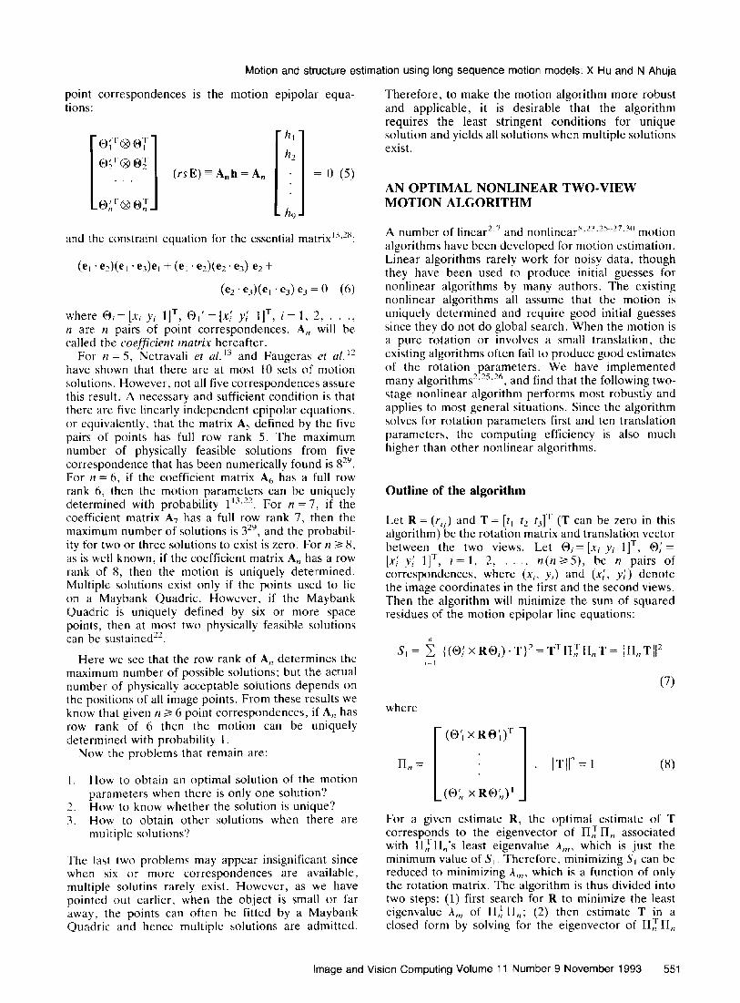
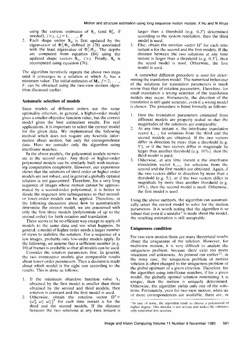
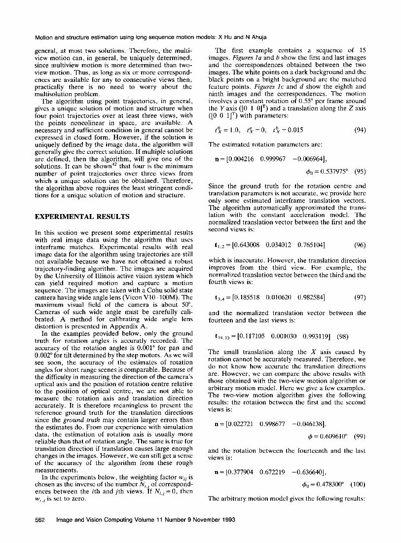
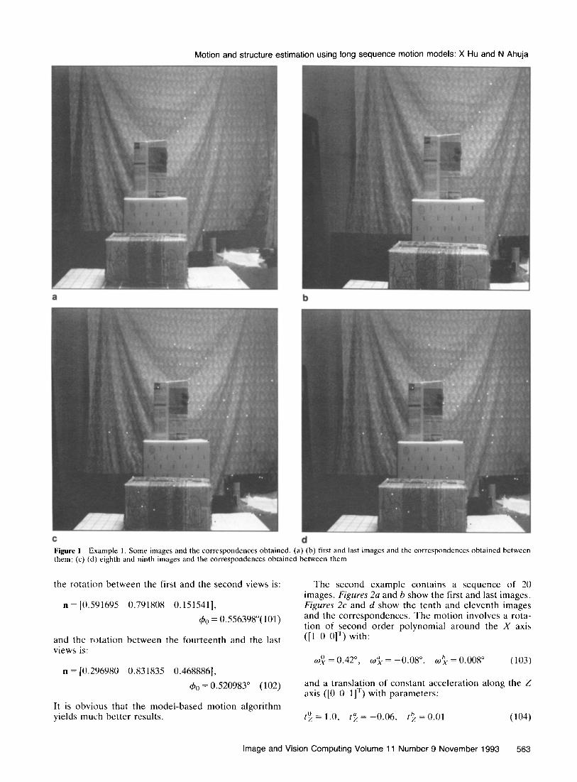
The first example contains a sequence of 15 images. Figures la and b show the first and last images and the correspondences obtained between the two images. The white points on a dark background and the black points on a bright background are the matched feature points. Figures lc and d show the eighth and ninth images and the correspondences. The motion involves a constant rotation of 0.55” per frame around the Y axis ([0 1 OIT) and a translation along the Z axis ([0 0 llT) with parameters:

tO,=l.O, t”x=o, &=0.015

The estimated rotation parameters are:

(94)

n = [0.004216 0.999967 -0.0069641,

&J = 0.537975” (95)

EXPERIMENTAL RESULTS

In this section we present some experimental results with real image data using the algorithm that uses interframe matches. Experimental results with real image data for the algorithm using trajectories are still not available because we have not obtained a robust trajectory-finding algorithm. The images are acquired by the University of Illinois active vision system which can yield required motion and capture a motion sequence. The images are taken with a Cohu solid state camera having wide angle lens (Vicon VlO-100M). The maximum visual field of the camera is about 50”. Cameras of such wide angle must be carefully calibrated. A method for calibrating wide angle lens distortion is presented in Appendix A.

Since the ground truth for the rotation centre and translation parameters is not accurate, we provide here only some estimated interframe translation vectors. The algorithm automatically approximated the translation with the constant acceleration model. The normalized translation vector between the first and the second views is:

t,,* = [0.643008 0.034012 0.7651041 (96)

which is inaccurate. However, the translation direction improves from the third view. For example, the normalized translation vector between the third and the fourth views is:

t3,4 = [0.185518 0.010620 0.9825841 (97)

and the normalized translation vector between the fourteen and the last views is:

In the examples provided below, only the ground truth for rotation angles is accuratly recorded. The accuracy of the rotation angles is 0.001” for pan and 0.002” for tilt determined by the step motors. As we will see soon, the accuracy of the estimates of rotation angles for short range scenes is comparable. Because of the difficulty in measuring the direction of the camera’s optical axis and the position of rotation centre relative to the position of optical centre, we are not able to measure the rotation axis and translation direction accurately. It is therefore meaningless to present the reference ground truth for the translation directions since the ground truth may contain larger errors than the estimates do. From our experience with simulation data, the estimation of rotation axis is usually more reliable than that of rotation angle. The same is true for translation direction if translation causes large enough changes in the images. However, we can still get a sense of the accuracy of the algorithm from these rough measurements.

t,4,,5 = [0.117105 0.001030 0.9931191 (98)

The small translation along the X axis caused by rotation cannot be accurately measured. Therefore, we do not know how accurate the translation directions are. However, we can compare the above results with those obtained with the two-view motion algorithm or arbitrary motion model. Here we give a few examples. The two-view motion algorithm gives the following results: the rotation between the first and the second views is:

n = [0.022721 0.998677 -0.0461381.

4 = 0.609610“ (99)

and the rotation between the fourteenth and the last views is:

In the experiments below, the weighting factor Wij is chosen as the inverse of the number Ni,j of correspondences between the ith and jth views. If Ni,j= 0, then Wi,j is set t0 zero.

n = [0.377904 0.672219 -0.6366401,

+, = 0.478300” (100)

The arbitrary motion model gives the following results:



a b

d

Figure 1 Example 1. Some images and the correspondences obtained. (a) (b) first and last images and the correspondences obtained between them; (c) (d) eighth and ninth images and the correspondences obtained between them

the rotation between the first and the second views is:

n = [Cl.591695 0.791808 0.151541],

C& = 0.556398”(101)

and the rotation between the fourteenth and the last views is:

n = [0.296980 0.831835 0.4688861,

+a = 0.520983” (102)

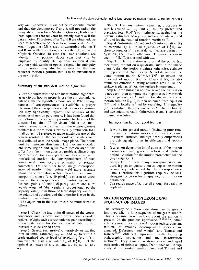
The second example contains a sequence of 20 images. Figures 2a and b show the first and last images. Figures 2c and d show the tenth and eleventh images and the correspondences. The motion involves a rotation of second order polynomial around the X axis ([l 0 Ojr’) with:

w; = 0.42”, w”x = -0.08”, w”x = 0.008 (103)

and a translation of constant acceleration along the Z axis ([0 0 llT) with parameters:

It is obvious that the model-based motion algorithm yields much better results. t; = 1.0. t> = -0.06, ts = 0.01 (104)


Motion and structure estimation using long sequence motion mot gels: X Hu and N Ahuja

a b

d

Figure 2 Example 2. Some images and the correspondences obtainea. (a) (b) first and last images; (c) (d) tenth and eleventh images and the correspondences obtained between them

The rotation also causes a small translation along the Y axis since the rotation centre is not at the optical centre. The estimated rotation parameters are:

and the interframe translation direction vectors are, for example:

t ,,2 = [0.034507 0.066768 0.9971721 (106)

t ,o,, , = [0.027467 0.123701 0.9919391 (107)

t ,9.20 = [0.008584 0.177239 0.9841301 (108)

0.008151

fib= [ -0.000314 1 0.000300

564 Image and Vision Computing Volume 11

Only two interframe translations are not accurate,

(105) which are:

t ,,* = [0.342731 0.311376 0.8863301 (109)

Number 9 November 1993


a b

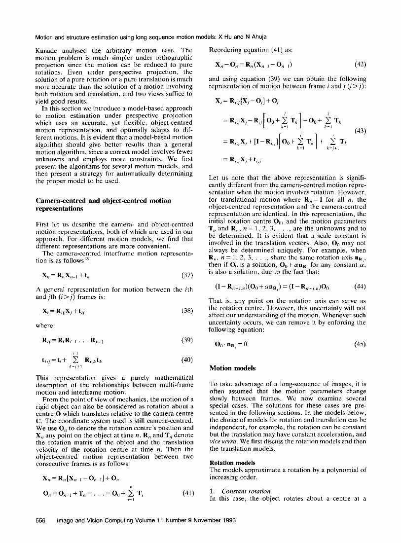
d Figure 3 Example 3. Some images and the correspondences obtained. (a) (b) first and last images and the correspondence’; obtained between them; (c) (d) tenth and eleventh images and the correspondences obtained between them

t ,,, ,x = [ -0.259094 -0.682176 (I.6837441 (110)

axis ([0 1 (I]“) with:

6J$ = 0.5”. W”v = 0.04”. LO’; = -0.03” (111)

The estimate of interframe translation vectors is more vulnerable to noise in the image data. We are finding methods to improve the accuracy of estimation of

and a translation of constant acceleration along X axis ([l 0 O]“) with parameters:

translation. The third examole also contains a seauence of 20 t’.;, = 1 .O, t”x = -0.04286 (112)

1 1

images. Figures 3a and b show the first and last images and the correspondences obtained between the two images. Figures 3c and d show the tenth and eleventh images and the correspondences. The motion involves a rotation of second order polynomial around the Y

However, in this example, the rotation causes a translation along the 2 axis that is comparable with the translation along the X axis. Therefore, we do not know the ground truth of the translation directions.



a b

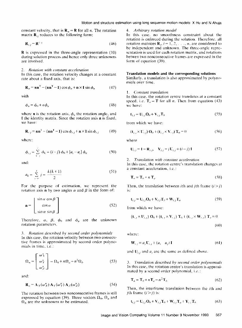
c d Figure 4 Example 4. Some images and the correspondences obtained. (a) and (b) first and last images; (c) (d) eighth and ninth images and the correspondences obtained between them

The estimated rotation parameters are:

slo= [~;;~~zzzJ n,= [ ;zzL3;;] )

The accuracy of this and the next example is worse than the first two examples. The main reason is probably due to the fact that the objects in this and the next example are further away, and the translation contains a component along the X axis which can be easily confused with rotation. However, for most time

0.017744

[ I

instants, the estimated rotation parameters are very close to the ground truth.

anb = -0.002894 (113) In the fourth example, 15 images are taken by a

0.000046 moving camera. Figures 4a and b show the first and last images. No correspondences are found between these

The estimates of the interframe translations are two images because of the large motion between them. omitted here for this example. Figures 4c and d show the eighth and ninth images and



the correspondences. The motion involves a rotation (tilt) with constant acceleration around the X axis ([l 0 OIT) with &= 0.6” per frame and +a = 0.04 per frame, and a constant translation along the X axis ([l 0 OIT). The rotation also causes a translation along % and Y axes, the amount of which is not accurately measured. The estimated rotation parameters are:

n = [0.970392 -0.197587 0.1389171 (114)

4” = 0.637189”, 4, = 0.041694” (115)

Due to image noise, the algorithm chooses a second order polynomial to estimate the translation parameters. Here we present a few interframe translation direction vectors:

t ,,* = IO.416507 -0.741442 -0.526104] (116)

t 7,x = [0.520486 -0.782628 -3414501 (117)

and:

t ,4. ,5 = [cl.649293 -0.758120 0.060604] (118)

Clearly, the translation vectors in this example are much less accurate than those in the first two examples. We are currently developing methods to evaluate and improve this accuracy.

SUMMARY

In this paper, we have presented a long sequence motion algorithm using the most appropriate of a set of motion models and a nonlinear two-view motion algorithm for estimating motion parameters from a

long sequence of images. These algorithms utilize the state-of-the-art techniques developed by many motion researchers and are very easy to use. The whole process, from feature detection to matching and then to motion estimation, is fully automated. The application of the algorithms to real image data has yielded good results, from which we can conclude that model-based methods yield much better results than those assuming arbitrary motions.

The algorithms in this paper can use either interframe matches or point trajectory points as input. Because the number of structure parameters does not increase with the number of image frames, trajectories contain much more information than interframe correspondences. Therefore, the accuracy of motion algorithms should be better if trajectories of points are used. Nevertheless, the results obtained using interframe matches over no more than 20 image frames are good enough for many applications.

APPENDIX A: CALIBRATING A WIDE-ANGLE LENS

In this appendix we present a simple method for calibrating wide angle lens cameras. This method is based on the assumption that the distortion is symmetric around the optical centre. Figure Au is a grid image taken with an uncalibrated camera, where we see straight lines are distorted into curves. The problem of calibration is to restore the curves to straight lines. To do this, we use a stretching function. defined below, to stretch the warped lines:

r’ = r(1 +cur+/3?) (Al)

where r is the distance of a point to the optical centre (x,,, yo) before calibration, and r’ is the calibrated

~_, . . , ...r_,..”

Figure Al Calibration of a wide angle lens camera. (a) Grid image of straight lines taken with uncalibrated camera; (b) same image after calibration


distance. We need to optimize four unknowns, (Y, /3, x0 and y0 such that the warped lines become mostly straight. The objective function used in the optimization process follows. Assume there are N horizontal and M vertical lines.

First, we rewrite equations (5) or (7) as:

S, = i {O;T(TxR)Oi}2=hTA~A,h i=l

First, the N x M intersection points of the lines in the uncalibrated image are identified. Then, the positions of the grid points on each horizontal line are fitted by a quadratic function:

y=yh+a,x+a2x* (A2)

where x is the horizontal coordinate of a point and y the vertical coordinate. Yh, a, and a2 are optimized for each horizontal line. Similarly, a quadratic function of the form:

x=x,+b,,+&y2 (A3)

is used to fit grid points on vertical lines. The NX M intersection points of the quadratic curves are the refined positions of the grid points and are to be used for calibrating the parameters (Y, p, x0 and y,.

For each choice of (Y, p, x0 and y. we find the least squares line fit to the refined grid points on horizontal or vertical curves. That is, for each curve (horizontal or vertical), we find a line:

where h = rsE. In the above equation we force 11 h1l2 = 2 so that the corresponding solution of T below satisfies IIT /I2 = 1. The optimal solution of h that minimizes S, corresponds to the eigenvector of ATA, associated with its smallest eigenvalue. Although the sign of h is uncertain, this uncertainty will not affect the decomposition discussed below. Then the goal below is to estimate a unit translation vector T and a rotation matrix T such that I/E-TX R)j2 is minimized, where the (Frobenius or Euclid) norm of a matrix is defined as the sum of its squared elements. In general, an essential matrix will have two decomposi- tions of the form TXR, which constitute a twisted pair*. However, only one decomposition yields positive depths for the correspondence data. The following method finds the solution that yields positive depths for

‘h~tc~r?~n~~~~‘4 that if (T, R) is the optimal decomposition of E, then T corresponds to the eigenvector of ETE associated with its least eigenvalue subject to //T/l* = 1. Therefore, T is the linear least squares solution of the following equation:

I& 12 m Y ll’= 0 (A4) ETT = ET[t, t2 f31T = 0 032)

such that the sum of its squared distances to the grid points related to that curve is minimized. The optimal solution of LY, 6, x0 and y. is that which minimizes the N+ 1w sums of squared distances.

To determine if T or -T is the right solution, we need make use of the correspondence data. Let:

Figure Alb is the calibrated image of Figure Ala, where we see that the lines are almost straight. This simple method is easy to apply and gives reasonable accuracy.

TX=[_t -1 -;] = G=[ ;;] (B3)

It is unfortunate that symmetry assumption is not true for all cases. Therefore, the results would be better if the image is divided into regions and the calibration is done piecewise. But this requires a more complicated method and more parameters to search for so that a globally optimal estimation of the parameters is often impossible. For the problem of motion estimation, we find that as long as a wide angle lens camera is used, the estimation accuracy is not so sensitive to the camera parameters. Therefore, the calibration method presented here should satisfy many purposes.

Then from the motion equation:

we would have:

TX (O’,Z:) = (TX R) OjZi, or

Irrespective of whether T or -T is the right solution, Z:iZ, can be determined by:

APPENDIX B: LINEAR TWO-VIEW MOTION ALGORITHMS Z: J Although linear solutions cannot be superior to nonlinear solutions, linear algorithms may give a very good starting point for nonlinear algorithms.

Let:

When the surface is not a ~aybank Quadric, we can first solve the essential matrix E = TX R linearly and then decompose E into T and R. Among the linear algorithms2,7,34, Philip’s Singular Value Decomposition (SVD) algorithm is optimal in the sense of least squares. Here we present severai simpler solutions.

Motion and structure estima!ion using long sequence motion models: X Hu and N Ahuja


(Bl)

(B4)

W)

036)

(B7)

(BS)


interpretations of a moving plane , J. Opt. Sot. Amer. A. Vol 7 (1990) Cui, N, Weng, J and Cohen. P ‘Extended structure and motion analysis from monocular image sequences’. Proc. Srd ICCV, Osaka, Japan (1990) pp 222-229 Broida, T and Chellapa, R ‘Estimating the kinematics and structure of a rigid object from a sequence of monocular images’. IEEE Trans. PAMI, Vol 13 No 6 (1991) pp 497-513 Young, G and Chellapa, R ‘Monocular motion estimation using a longsequence of noisy images’. Proc. Int. Conf. on Acoustics, Soeech and Sianal Processina, Toronto. Canada, Vol 4 (1991) pi 2437-2440 - Young, G and Chellapa, R ‘3-D motion estimation using a sequence of noisy stereo images: models. estimation, and uniqueness results’. IEEE Trans. PAMI. Vol 12 No 8 (1990) pp 735-759

then if L, < Lz, T is the correct solution; else we must have L2 < L, and -T is the correct solution. We denote the correct solution as T in the below.

After T is determined, we need to estimate R such that J/E-TxR~\~ or IIE~-R~G~I~ is minimized. The algorithms40.4’ can then be applied to obtain the optimal solution of R. For motion of small rotations, the rotation angles can also be solved for from equation (20) in a closed form.

ACKNOWLEDGEMENTS

The support of National Science Foundation and Defense Advanced Research Projects Agency under grant IRI-89-02728, and the US Army Advanced Construction Technology Center under grant DAAL 03-87-K-0006, is gratefully acknowledged.

REFERENCES

1

2

3

4

5

6

7

8

9

10

11

12

13

14

15

16

17

Longuet-Higgins, H ‘A computer algorithm for reconstructur- ing a scene from two projections’, Nature, Vol 293 (1981) pp 133-13s Tsai, R and Huang, T ‘Uniqueness and estimation of three- dimensional motion parameters of rigid objects with curved surfaces’, lEEE Trans. PAMI, Vol 6 No 1 (1984) pp 13-26 Tsai, R, Huang, T and le Zhu, W ‘Estimating three-dimensional motion parameters of a rigid planar patch, II: Singular value decomposition’, IEEE Trans. Accoust., Speech and Signal Process.. Vol 30 No 4 (1982) pp 525-534 Longuet-Higgins, H ‘The visual ambiguity of a moving plane’. Proc. Roval Sot. Lond., Series B, Vol 223 (1985) pp 165-175 Longuet-Higgins, H ‘The reconstruction of a plane surface from two perspective projection’, Proc. Royal Sot. Lond., Series B. Vol 227 (1986) pp 399-410 Longuet-Higgins; H ‘Multiple interpretations of a pair of images of a surface’, Proc. Royal Sot. Lond., Series B. Vol 223 (1988) pp 165-175 Zhuang, X, Huang, T and Haralick, R ‘Two-view motion analvsis: A unified aleorithm’. Oat. Sot. Amer.. Vol 3 No 9 (198;i) pp 1492-1500 - . Horn, B ‘Relative orientation’, Proc. Image Understanding Workshop, Irvine, CA (1989) pp 826-837 Horn, B ‘Motion fields are hardly ever ambiguous’, Int. J. Computer Vision, Vol 1 (October 1987) Weng, J, Ahuja, N and Huang, T ‘Motion and structure from point correspondences: A robust algorithm for planar case with error estimation’, Proc. Int. Conf. on Pattern Recognition, Paris, France (1988) Hu, X and Ahuja, N ‘A robust algorithm for plane motion solution’, Proc. Int. Conf. on Automation, Robotics and Computer Vision. Singapore (1990) Faugeras, 0 and Maybank, S ‘Motion from point matches: multiplicity of solutions’, Proc. IEEE Workshop on Visual Motion. Irvine, CA (1989) pp 248-255 Netravali. A. Huane. T. Krishnakumar, A and Holt. R ‘Algebraic methods i’l 3-D motion estimation from two-view point correspondence’, Int. .I. Imaging Syst. & Technol., Vol 1 (1989) pp 78-99 Negahdaripour, S ‘Multiple interpretations of the shape and motion of objects from two perspective images’, IEEE Trans. PAMI, Vol 12 No 11 (1990) pp 1025-1039 Negahdaripour, S ‘Ambiguities of a motion field’, Proc. 1st Int. Conf. Comput. Vision, London, UK (1987) pp 607-61 I Negahdaripour, S ‘Critical surface pairs and triplets’, Int. J. Comput. Vision, Vol 3 (1989) Negahdaripour. S ‘Closed-form relationship between the two

18

19

20

21

22

23

24

2s

26

27

28

2’)

30

31

32

33

34

35

36

37

38

3Y

40

41

42

Hu, X and Ahuja. N ‘Sufficient conditions for double or unique solution of motion and structure’, Proc. Int. C’onf. on Acoustics, Speech and Signal Processing. Toronto. Canada. Vol 4 (lY91) pp 2445-2448 (To appear in C\‘GIP: Image Understanding, July 1993) Roach, J and Aggarwal. J K ‘Determining the movcmcnt of objects from a sequence of images’. J. ACM. Vol 6 (lY80) pp 554-562 Yen. B and Huang. T ‘Dctcrminlng the 3-D motion and structure of a rigid object using spherical projections’, Comput. Vision, Graph. & Image Process., Vol 21 (1983) pp 21-32 Spetsakis, M and Aloimonos, J ‘Optimal computing of structure from motion using point correspondences in two frames’, Proc. Ist ICCV, Tampa, FL (1988) pp 449-453 Weng, .I, Ahuja, N and Huang. T S ‘Closed-form solution+ maximum likelihood: A robust approach to motion and structure estimation’. Proc. CVPR, Ann Arbor. MI (1988) pp 381-386 Jcrian, C and Jain, R ‘Polynomial methods for structure from motion’, Proc. 1st ICCV, Tampa, FL (1988) pp 197-206 Huang, T and Faugeras. 0 ‘Some properties-of the E matrix in two-view motion estimation’. IEEE Trans. PAMI. Vol I I No 12 (1989) pp 1310-1312 Faugeras. 0 and Maybank, S ‘Motion from point matches: multiplicity of solutions’, Inr. J. (‘omputer Vision. Vol 4 (1990) pp 225-246 Weng, J, Huang. T and Ahuja. N ‘Motion and structure from two perspective views: Algoiithms. error analysis. and error estimation’. IEEE Trans. PA Ml. Vol I I No 5 ( 198’)) pp 45 I-476

Hooke. R and Jeeves. T “‘Direct Search Sol;tion”,‘c;f numerical and statistical problems’. J. .A(‘M (1961) pp 212-22’) Wilder, D and Beightler. C Foundations of Optimizution. Prentice-Hall, Englewood Cliffs, NJ (1967) Iu. S-L and Wohn, K ‘Estimation of general rigid motion from a long sequence of images’. Proc. ICPR, Atlantic City, NJ (1990) pp 217-219 Philip, J ‘Estimation of three-dimensional motion of rlgid objects from noisy observations’. IEEE Truns. PAMI, Vol 13 No 1 (1991) pp 61-66 Aloimonos. J ‘Purposive and qualitative active vision’. Proc. Int. Joint Conf. on Pattern Recognition (IYYO) pp 346-360 Weng, J, Huang, T and Ahuja, N ‘3-D motion estimation. understanding. and prediction from noisy image sequences’. IEEE Trans. PAMI, Vol 9 No 3 (1987) pp 370-3XY Debrunner, C and Ahuja. N ‘A direct data approximation based motion estimation algorithm’, Proc. l&h Int. Conf. on Pattern Recognition. Atlantic Citv. NJ (19YO) pp 384-38’) Tomasi, C and Kanade, ‘T. ‘Shape and motion without depth‘, Proc. 3rd ICCV. Osaka. Japan (1YYO) pp 91-9.5 Tomasi, C and Kanade. T ‘The factorization method for the recovery of shape and motion from image streams’, Image Understandine Work&on. San Diego. CA (lYY2) PP 459-472 Faugeras, 0 ind Heberi. M ‘A 3.Grecog&ion and positioning algorithm using geometrical matching between primitive surfaces’, fnt. Joint Conf. on Artif. Intell. Karlsruhe. Germany (1983) DD 996-1001 irun; i<: Huang, T and Blostcin, S ‘Least squares fitting of two 3-D noint sets’. IEEE Trans. PA MI. Vol I I (1987) pp 69X-700 Hu, ‘X Perception of Shape and Motion, PhD &sertation. Department of Electrical and Computer Engineering, University of Illinois, Urbana. IL. (1993)


motion and structure estimation using long sequence …vision.ai.illinois.edu/publications/motion...

Documents