motion and optical flow - university of michiganjjcorso/t/598f14/files/lecture_1015... · motion...
TRANSCRIPT

Motion and Optical Flow
Instructor: Jason Corso (jjcorso)!web.eecs.umich.edu/~jjcorso/t/598F14!
!
Materials on these slides have come from many sources in addition to myself. !Many are adaptations from Savarese, Lazebnik, Darrell, Hager, Pollefeys, Seitz, Szeliski, Saenko and Grauman. !Individual slides reference specific sources when possible.!
EECS 598-08 Fall 2014!Foundations of Computer Vision!!
Readings: FP 10.6; SZ 8; TV 8!Date: 10/15/14!!

2
https://www.youtube.com/watch?v=BDtvjKMl30w!

3
https://www.youtube.com/watch?v=5rR_9YIcg_s!

Plan
• Motion Field!• Patch-based / Direct
Motion Estimation!• (Next: Feature Tracking)!• (Next: Layered Motion ! Models)!
• External Resource:!– Mubarak Shah’s lecture on optical flow!
• http://www.youtube.com/watch?v=5VyLAH8BhF8!
4

Video
• A video is a sequence of frames captured over time • Now our image data is a function of space
(x, y) and time (t)
Slide adapted from K. Grauman.!
5

Motion field
• The motion field is the projection of the 3D scene motion into the image
Slide adapted from K. Grauman; images from Russel and Norvig.!
6
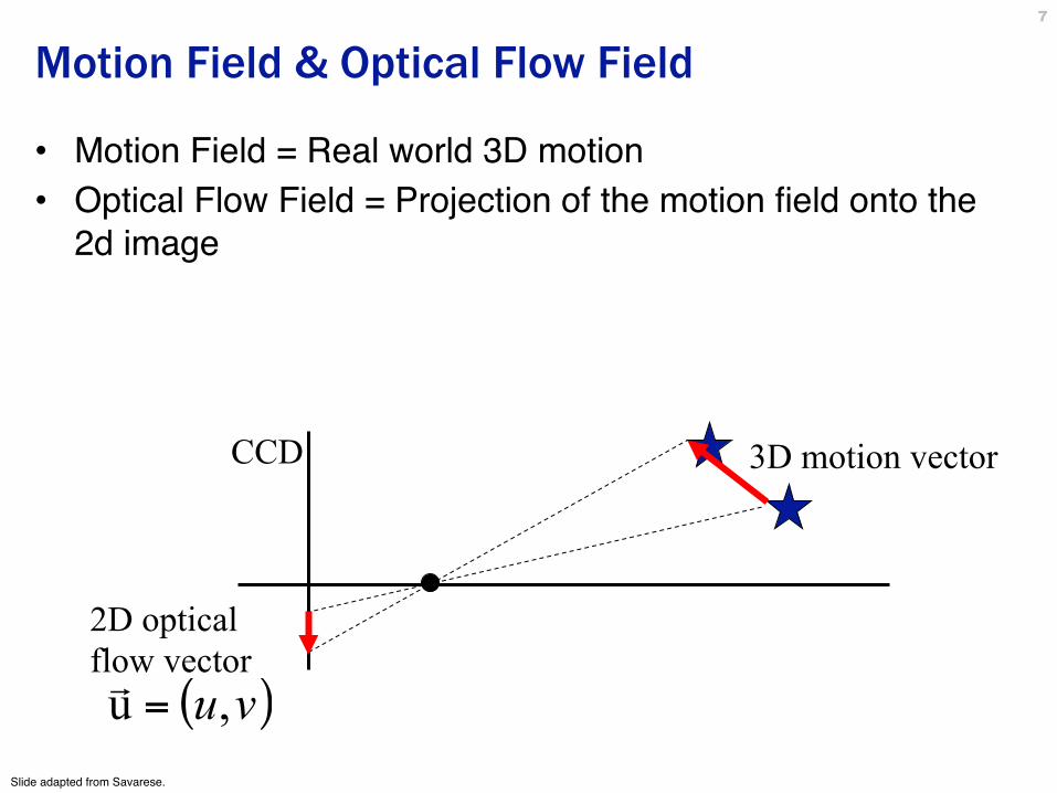
Motion Field & Optical Flow Field
• Motion Field = Real world 3D motion !• Optical Flow Field = Projection of the motion field onto the
2d image!
3D motion vector
2D optical flow vector
( )vu,u =!
CCD
Slide adapted from Savarese.!
7

Motion field and parallax • P(t) is a moving 3D point • Velocity of scene point: V =
dP/dt • p(t) = (x(t),y(t)) is the
projection of P in the image • Apparent velocity v in the
image: given by components vx = dx/dt and vy = dy/dt
• These components are known as the motion field of the image p(t)
p(t+dt)
P(t) P(t+dt)
V
v
Slide adapted from K. Grauman.!
8

Motion field and parallax
p(t) p(t+dt)
P(t) P(t+dt)
V
v
),,( Zyx VVV=V
2ZVZf zPVv −
=
Zf Pp =
To find image velocity v, differentiate p with respect to t (using quotient rule):
ZxVVfv zx
x−
=Z
yVVfv zyy
−=
Image motion is a function of both the 3D motion (V) and the depth of the 3D point (Z)!
Quotient rule: D(f/g) = (g f’ – g’f)/g^2
Slide adapted from K. Grauman.!
9

Motion field and parallax
• Pure translation: V is constant everywhere Z
xVVfv zxx
−=
ZyVVf
v zyy
−=
),(1 0 pvv zVZ−=
( )yx VfVf ,0 =v
Slide adapted from K. Grauman.!
10

Motion field and parallax
• Pure translation: V is constant everywhere
• Vz is nonzero: – Every motion vector points toward (or away from) v0,
the vanishing point of the translation direction
),(1 0 pvv zVZ−=
( )yx VfVf ,0 =v
Slide adapted from K. Grauman.!
11

Motion field and parallax
• Pure translation: V is constant everywhere
• Vz is nonzero: – Every motion vector points toward (or away from) v0,
the vanishing point of the translation direction • Vz is zero:
– Motion is parallel to the image plane, all the motion vectors are parallel
• The length of the motion vectors is inversely proportional to the depth Z
),(1 0 pvv zVZ−=
( )yx VfVf ,0 =v
Slide adapted from K. Grauman.!
12
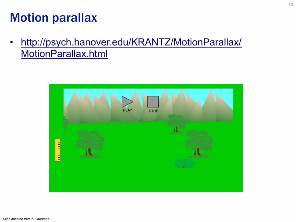
Motion parallax
• http://psych.hanover.edu/KRANTZ/MotionParallax/MotionParallax.html
Slide adapted from K. Grauman.!
13

Figure from Michael Black, Ph.D. Thesis
Length of flow vectors inversely proportional to depth Z of 3d point
points closer to the camera move more quickly across the image plane
Motion field + camera motion
Slide adapted from K. Grauman.!
14

Motion field + camera motion
Zoom out! Zoom in! Pan right to left!
Slide adapted from Savarese and Grauman.!
Forward motion! Rotation! Horizontal translation!
Closer objects appear to move faster!!!
15

Motion estimation techniques • Feature-based methods
– Extract visual features (corners, textured areas) and track them over multiple frames
– Sparse motion fields, but more robust tracking – Suitable when image motion is large (10s of pixels)
• Direct methods – Directly recover image motion at each pixel from spatio-
temporal image brightness variations – Dense motion fields, but sensitive to appearance variations – Suitable for video and when image motion is small
Slide adapted from K. Grauman.!
16

Optical flow
• Definition: optical flow is the apparent motion of brightness patterns in the image
• Ideally, optical flow would be the same as the motion field • Have to be careful: apparent motion can be caused by
lighting changes without any actual motion
Slide adapted from K. Grauman, Zelnik-Manor, Savarese.!
Where did each pixel in image 1 go to in image 2!
17

Motion Field & Optical Flow Field
• Motion Field = Real world 3D motion !• Optical Flow Field = Projection of the motion field onto the
2d image!
3D motion vector
2D optical flow vector
( )vu,u =!
CCD
Slide adapted from Savarese.!
18

Optical Flow
Pierre Kornprobst's Demo !
Slide adapted from Savarese.!
19

When does it break?
The screen is stationary yet displays motion!
Homogeneous objects generate zero optical flow.!
Fixed sphere. Changing light source.!
Non-rigid texture motion!
Slide adapted from Savarese.!
20

Apparent motion ~= motion field
Figure from Horn book Slide adapted from K. Grauman.!
21

The Optical Flow Field
Still, in many cases it does work….!
• Goal:Find for each pixel a velocity vector which says:!– How quickly is the pixel moving across the image!– In which direction it is moving!
( )vu,u =!
Slide adapted from Savarese.!
22

Estimating optical flow
• Given two subsequent frames, estimate the apparent motion field between them.
• Key assumptions!• Brightness constancy: projection of the same point looks the
same in every frame!• Small motion: points do not move very far!• Spatial coherence: points move like their neighbors!
I(x,y,t–1) I(x,y,t)
Slide adapted from K. Grauman.!
23
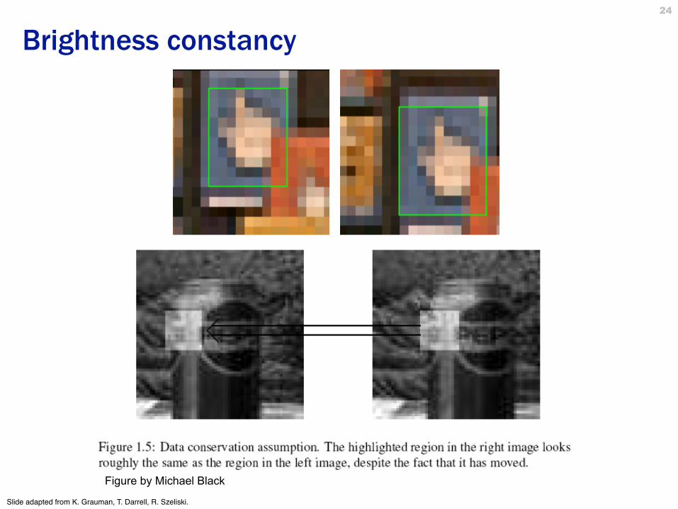
Brightness constancy
Slide adapted from K. Grauman, T. Darrell, R. Szeliski.!
Figure by Michael Black
24

• Brightness Constancy Equation:
),()1,,( ),,(),( tyxyx vyuxItyxI ++=−
),(),(),,()1,,( yxvIyxuItyxItyxI yx ⋅+⋅+≈−
Can be written as:!
The brightness constancy constraint
I(x,y,t–1) I(x,y,t)
0≈+⋅+⋅ tyx IvIuISo,!Slide adapted from K. Grauman.!
25

The brightness constancy constraint
• How many equations and unknowns per pixel? – One equation, two unknowns
• Intuitively, what does this constraint mean?!
• The component of the flow perpendicular to the gradient (i.e., parallel to the edge) is unknown!
0=+⋅+⋅ tyx IvIuI
0),( =+⋅∇ tIvuI
Slide adapted from K. Grauman.!
26

The brightness constancy constraint
• How many equations and unknowns per pixel? – One equation, two unknowns
• Intuitively, what does this constraint mean?!
• The component of the flow perpendicular to the gradient (i.e., parallel to the edge) is unknown!
0=+⋅+⋅ tyx IvIuI
0)','( =⋅∇ vuI
edge
(u,v)
(u’,v’)
gradient
(u+u’,v+v’)
If (u, v) satisfies the equation, so does (u+u’, v+v’) if !
0),( =+⋅∇ tIvuI
Slide adapted from K. Grauman.!
27

The aperture problem
Perceived motion
Slide adapted from K. Grauman.!
28

The aperture problem
Actual motion
Slide adapted from K. Grauman.!
29

The barber pole illusion
http://en.wikipedia.org/wiki/Barberpole_illusion!Slide adapted from K. Grauman.!
30

The barber pole illusion
http://en.wikipedia.org/wiki/Barberpole_illusion!Slide adapted from K. Grauman.!
31

The barber pole illusion
http://en.wikipedia.org/wiki/Barberpole_illusion!Slide adapted from K. Grauman.!
32
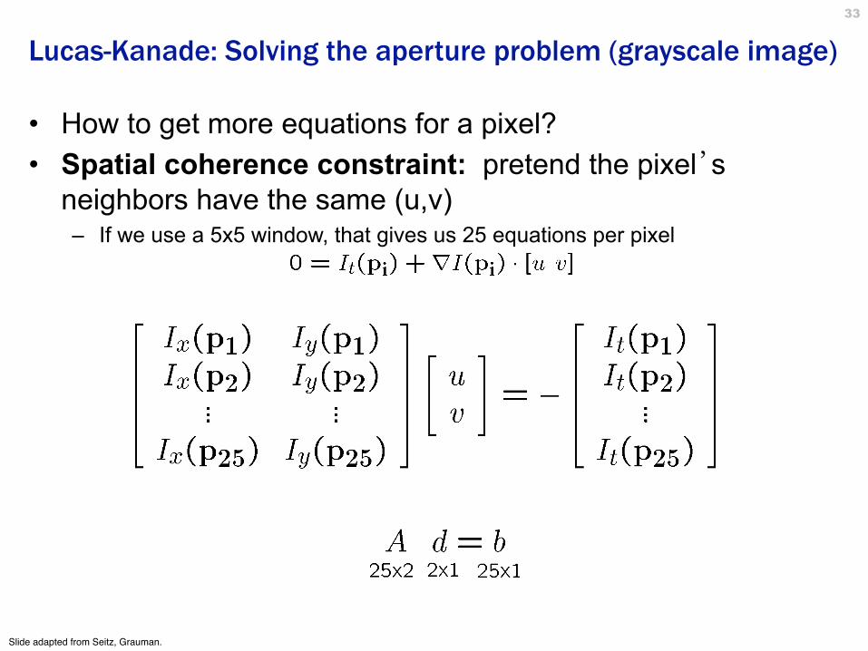
Lucas-Kanade: Solving the aperture problem (grayscale image)
• How to get more equations for a pixel? • Spatial coherence constraint: pretend the pixel’s
neighbors have the same (u,v) – If we use a 5x5 window, that gives us 25 equations per pixel
Slide adapted from Seitz, Grauman.!
33

Lucas-Kanade: Solving the aperture problem Prob: we have more equations than unknowns
• The summations are over all pixels in the K x K window!• This technique was first proposed by Lucas & Kanade (1981)!
Solution: solve least squares problem!• minimum least squares solution given by solution (in d) of:!
Slide adapted from Seitz, Grauman.!
34

Conditions for solvability
When is this solvable?!• ATA should be invertible !• ATA should not be too small!
– eigenvalues λ1 and λ2 of ATA should not be too small!• ATA should be well-conditioned!
– λ1/ λ2 should not be too large (λ1 = larger eigenvalue)!
Slide adapted from Seitz, Grauman.!
Look Familiar?!
35

Conditions for solvability
λ1
λ2
“Corner” λ1 and λ2 are large, λ1 ~ λ2; E increases in all directions
λ1 and λ2 are small; E is almost constant in all directions
“Edge” λ1 >> λ2
“Edge” λ2 >> λ1
“Flat” region
Classification of image points using eigenvalues of M:!
Source: Kokkinos, Saverese.!
36

37

Edge
– gradients very large or very small!– large λ1, small λ2!
Slide adapted from Seitz, Grauman.!
38

Low-texture region
– gradients have small magnitude!– small λ1, small λ2!
Slide adapted from Seitz, Grauman.!
39

High-texture region
– gradients are different, large magnitudes!– large λ1, large λ2!
Slide adapted from Seitz, Grauman.!
40

Can we measure optical flow reliability?
• Can we measure “quality” of optical flow in regions from just a single image?!
• High Quality / Good features to track:!• - Harris corners (guarantee small error sensitivity)!
• Poor Quality / Bad features to track:!• - Image points when either λ1 or λ2 (or both) is small (i.e., edges or
uniform textured regions)!
Slide adapted from Savarese.!
41

Iterative Refinement
• Estimate velocity at each pixel using one iteration of Lucas and Kanade estimation!
• Warp one image toward the other using the estimated flow field!(easier said than done)!
• Refine estimate by repeating the process!
Slide adapted from Szeliski.!
42

Optical Flow: Iterative Estimation
x!x0!
Initial guess: Estimate:
estimate update
(using d for displacement here instead of u)
Slide adapted from Szeliski.!
43

Optical Flow: Iterative Estimation
x!x0!
estimate update
Initial guess: Estimate:
Slide adapted from Szeliski.!
44

Optical Flow: Iterative Estimation
x!x0!
Initial guess: Estimate: Initial guess: Estimate:
estimate update
Slide adapted from Szeliski.!
45

Optical Flow: Iterative Estimation
x!x0!
Slide adapted from Szeliski.!
46

Optical Flow: Iterative Estimation
• Some Implementation Issues:!– Warping is not easy (ensure that errors in warping are smaller
than the estimate refinement)!– Warp one image, take derivatives of the other so you don’t
need to re-compute the gradient after each iteration.!– Often useful to low-pass filter the images before motion
estimation (for better derivative estimation, and linear approximations to image intensity)!
Slide adapted from Szeliski.!
47

Optical Flow: Aliasing
Temporal aliasing causes ambiguities in optical flow because images can have many pixels with the same intensity. I.e., how do we know which ‘correspondence’ is correct?
nearest match is correct (no aliasing)
nearest match is incorrect (aliasing)
To overcome aliasing: coarse-to-fine estimation.
actual shift
estimated shift
Slide adapted from Szeliski.!
48

Limits of the gradient method
Fails when intensity structure in window is poor!Fails when the displacement is large (typical operating
range is motion of 1 pixel)!Linearization of brightness is suitable only for small
displacements!• Also, brightness is not strictly constant in images!
actually less problematic than it appears, since we can pre-filter images to make them look similar!
Slide adapted from Szeliski.!
49

image I!image J!
a!Jw!warp! refine!
a! aΔ !+!
Pyramid of image J! Pyramid of image I!
image I!image J! u=10 pixels!
u=5 pixels!
u=2.5 pixels!
u=1.25 pixels!
Coarse-to-Fine Estimation
Slide adapted from Szeliski.!
50

J! Jw! I!warp! refine!ina!
a!Δ+!
J! Jw! I!warp! refine!
a!
a!Δ+!
J!
pyramid !construction!
J! Jw! I!warp! refine!
a!Δ+!
I!
pyramid !construction!
outa!
Coarse-to-Fine Estimation
Slide adapted from Szeliski.!
51
Applications of Optical Flow
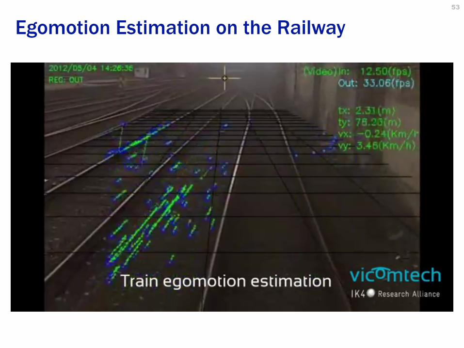
Egomotion Estimation on the Railway 53

Applications to Segmentation
• Background subtraction – A static camera is observing a scene – Goal: separate the static background from the moving
foreground
How to come up with background frame estimate without access to “empty” scene?
Slide adapted from K. Grauman.!
54
Applications to Segmentation
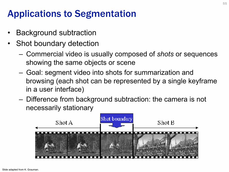
• Background subtraction • Shot boundary detection
– Commercial video is usually composed of shots or sequences showing the same objects or scene
– Goal: segment video into shots for summarization and browsing (each shot can be represented by a single keyframe in a user interface)
– Difference from background subtraction: the camera is not necessarily stationary
Slide adapted from K. Grauman.!
55

Applications to Segmentation
• Background subtraction • Shot boundary detection
– For each frame • Compute the distance between the current frame and the
previous one – Pixel-by-pixel differences – Differences of color histograms – Block comparison
• If the distance is greater than some threshold, classify the frame as a shot boundary
Slide adapted from K. Grauman.!
56

Applications To Segmentation
• Background subtraction • Shot boundary detection • Motion segmentation
– Segment the video into multiple coherently moving objects
Slide adapted from K. Grauman.!
57
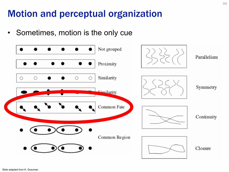
Motion and perceptual organization
• Sometimes, motion is the only cue
Slide adapted from K. Grauman.!
58

Motion and perceptual organization
• Sometimes, motion is foremost cue
Slide adapted from K. Grauman.!
59

Motion and perceptual organization
• Even “impoverished” motion data can evoke a strong percept
Slide adapted from K. Grauman.!
Sources: Maas 1971 with Johansson; downloaded from Youtube.!
60

Uses of motion • Estimating 3D structure • Segmenting objects based on motion cues • Learning dynamical models • Recognizing events and activities • Improving video quality (motion stabilization)
Slide adapted from K. Grauman.!
61

Crowd Analysis 62
http://www.vision.eecs.ucf.edu/projects/sali/CrowdSegmentation/Mecca_flowfield.wmv!

Aerial Vehicle Target Tracking 63
https://www.youtube.com/watch?v=C95bngCOv9Q!

A Camera Mouse
• Video interface: use feature tracking as mouse replacement
• User clicks on the feature to be tracked !• Take the 15x15 pixel square of the feature !• In the next image do a search to find the 15x15 region with the highest correlation !• Move the mouse pointer accordingly !• Repeat in the background every 1/30th of a second !!James Gips and Margrit Betke
http://www.bc.edu/schools/csom/eagleeyes/
64

A Camera Mouse
• Specialized software for communication, games
James Gips and Margrit Betke http://www.bc.edu/schools/csom/eagleeyes/
65

Optical Flow for Games! 66
https://www.youtube.com/watch?v=E7h4OaTtCzY!

Motion Paint: an example use of optical flow
http://www.fxguide.com/article333.html
Use optical flow to track brush strokes, in order to animate them to follow underlying scene motion.
67

68
Motion Paint: an example use of optical flow
https://www.youtube.com/watch?v=S5S_ABFcF_4!

Next Lecture: Tracking
• Readings: FP 10.6; SZ 8; TV 8!– Global, Parametric Motion Models.!
69