Mortality of Children and Parental

Disadvantage

Peng Yu*

Research and Analysis Branch

Department of Families, Community Services and Indigenous Affairs

* The author thanks Rebecca Kippen, Peter McDonald, and my colleagues at the Australian Government Department of Families, Community Services and Indigenous Affairs (FaCSIA) for helpful comments and suggestions. The data used for this research is constructed for an Australian Research Council (ARC) Linkage project – Intergenerational Transmission of Dependence on Income Support: Patterns, Causation and Implications for Australian Social Policy – which is partly funded by FaCSIA. However, the opinions, comments and/or analysis expressed in this document are those of the author and do not necessarily represent the views of the ARC, the Minister for Families, Community Services and Indigenous Affairs or the Australian Government Department of Families, Community Services and Indigenous Affairs, and cannot be taken in any way as expressions of Government policy.

1

Abstract

This paper investigates the underlying influencing factors of the premature death of

children, specifically looking at the correlation between mortality risk of children and

parental disadvantage at an individual level. Largely due to lack of appropriate data,

this issue is not well explored in Australia. This paper tries to fill in the gap by

creatively using a unique administrative dataset of FaCSIA, which contains

approximately a whole birth cohort of Australian children. The findings indicate that

the mortality of children is significantly correlated with several indicators of parental

disadvantage, such as Indigenous status, low income, long duration of income

support, teenage motherhood, and living in socio-economically disadvantaged areas.

This paper discusses how some measures of disadvantage, such as unemployment or

income support reliance used in isolation, may underestimate the extent of

intergenerational transmission of disadvantage, because children from disadvantaged

families are underrepresented in the samples of adults due to their high premature

mortality.

JEL Classification: J13; C41

Key Words: mortality; premature death; children; parent; disadvantage; socio-

economic; income support; Indigenous; Australia; intergenerational; non-parametric

2

1. Introduction

Premature death of children is a very adverse outcome and has significant impacts on

families. Children are the future of society; improving their health and especially

reducing their mortality not only directly affects the current wellbeing of children and

individual families, but also has long-lasting effects on their future prosperity, thus

contributes to the sustainable social and economic development of the nation as a

whole.

Australian children generally have good health and the mortality of children has been

falling for decades. In the last two decades, the death rates of children aged between

0-14 years have approximately halved (AIHW 2006).

However, compared with other countries in the Organisation for Economic Co-

operation and Development (OECD), the Australian infant mortality rates were only

at the middle level in 2003, and the ranking had even fallen since 1987. The ‘health

expenditure-to-GDP-ratio’ of Australia (11.6%) and health expenditure per person

($3,855) were both below the OECD weighted averages (11.6% and $4,035), and

governments’ contribution to total health expenditure (67.8%) was also four

percentage points below OECD unweighted average in 2003 (AIHW 2006).

To improve the health and reduce the mortality of children requires good knowledge

of the determinants of health and causes of mortality of children, while understanding

better the underlying influencing factors of mortality of children has more important

policy implications. The latter helps identify the high risk (focus) groups within the

population, and can help to find well-targeted solutions in preventing the occurrence

of the fatal diseases and injury, improving the response, and ultimately reducing the

mortality risk after the occurrence of the fatal diseases and injury.

Research shows that the incidence of diseases, injuries and mortality of children is not

randomly distributed; certain groups of the population, mostly the socio-economically

disadvantaged groups, are suffering significantly higher child mortality. For instance,

between 1999 and 2003 the mortality of Indigenous children was two to three times

higher than other children (ABS 2007), and children in very remote areas also had

approximately two times higher mortality than children in major cities (AIHW 2006).

3

The effects of family and social environment on health are well documented, but

unfortunately current data available in Australia is still very limited, which hinders the

ability to fully explain the influences of environmental factors on the health of

children (AIHW 2006). Aggregate data is mostly used in the existing studies and

findings are commonly based on direct tabulation without controlling for other

important influencing factors. Therefore, relative importance of the factors cannot be

compared.

One contribution of the current research is the use of a unique dataset – the Second

Transgenerational Data Set (TDS2) – to investigate the effects of family and social

environment on the mortality of children at an individual level. TDS2 consists of

nearly a whole birth cohort of Australian children, and contains rich information on

parents and children, including date of birth, date of death and welfare history. This

provides a very good opportunity for analysing influencing factors of premature

deaths of children and locating the leading factors.

Understanding the underlying influencing factors resulting in the premature death of

children is also important for other reasons. There is evidence of an intergenerational

transmission of disadvantage; that is, children brought up in disadvantaged families

are commonly observed to be more likely to experience adverse outcomes themselves,

such as poor education attainment, poor health, high unemployment, low income and

welfare reliance (Beaulieu et al 2001; Corak et al 2000; Gottschalk 1992; 1996;

Maloney and Pacheco 2003; Rank and Cheng 1995). In Australia, there are relatively

fewer studies on this issue, but there is similar evidence of intergenerational

transmission of disadvantage (McCoull and Pech 2000; Pech and McCoull 1998;

2000).

One problem about the current literature on intergenerational transmission of

disadvantage is that if the premature death of children is significantly correlated with

parental disadvantage, then the extent of intergenerational transmission of

disadvantage tends to be underestimated by indicators such as income support (IS)

reliance and unemployment. This is because premature deaths of children preclude

them from being unemployed or receiving income support as adults.

The results of the research reported in this paper show that the risk of premature death

is significantly higher for children from disadvantaged families, as indicated by

4

certain characteristics of parents, such as long income support duration, low income,

Indigenous status, teenage motherhood, disability, and living in socio-economically

disadvantaged or remote areas.

Overall, the findings suggest that premature death of children should not be neglected

as a significant adverse outcome of children in the research on intergenerational

transmission of disadvantage and in the policy arena. If we want to break the cycle of

intergenerational transmission of disadvantage, we should strive to reduce the

mortality of children from disadvantaged families in the first place.

The rest of the paper is structured as follows. The next section reviews relevant

literature and proposes a conceptual framework for this study. Section 3 briefly

introduces the data and the sample used for the research. Section 4 undertakes

descriptive analyses. Sections 5 and 6 report estimation results of logistic and duration

models, respectively. The last section concludes the paper with a summary and

discussion.

5

2. Literature Review and Conceptual Framework While the health of Australian children has been continuously improving, the

mortality of children has been continuously falling for all age groups, with boys

generally having higher mortality rates than girls. According to the Australian Bureau

of Statistics (ABS 2007), the proportion of children (under 15 years) with a long-term

health condition decreased from 44 percent in 2001 to 41 percent in 2005. From 1985

to 2005, the male infant mortality rates dropped from 11.4 to 5.4 per 1,000 live births;

the death rates of boys aged 1-4 years and 5-14 dropped from 0.6 to 0.3 and from 0.3

to 0.1 per 1000 population, respectively; and for young men aged 15-19 years the

death rates dropped from 1.1 to 0.5 (ABS 2006). The mortality rates of girls also

halved during the same period; the corresponding changes for girls in the four age

groups are respectively from 8.9 to 4.8, from 0.4 to 0.2, from 0.2 to 0.1, and from 0.4

to 0.2 (ABS 2006).

Mortality of children generally falls with age, with infants (under one year old) having

the highest mortality. In 2004, infant deaths accounted for 68 percent of all childhood

deaths (0-14 years); another 15 percent of deaths happened among children aged 1-4

years; and the remaining 17 percent were among children aged 4-14 years (ABS

2007).

2.1 The Direct Causes of Premature Death of Children A better understanding of the causes of death helps find better approaches for

reducing mortality and increasing life expectancy. This is especially important for

children, for whom most deaths are preventable.

Generally speaking, diseases and injury are the two main direct causes of premature

deaths of Australian children, while the causes of infant deaths are different from

those of older children.

For infant deaths in 2004, the leading causes included certain conditions originating in

the peri natal period (the period five months before and one month after birth),

congenital malformations, deformations and chromosomal abnormalities; in total,

these accounted for 71 percent of total infant deaths (ABS 2007). For children aged 1-

14 years, external causes (such as traffic accidents and assaults), cancer, and diseases

6

of the nervous system were the major causes of deaths (ABS 2007). For young people

aged 15-24 years, external causes (including traffic accidents and intentional self-

harm) were also the main cause of death, accounting for more than half of the total

deaths in the age group (AIHW 2006). As a leading cause of mortality and disability

of children, injury was identified as a priority issue by the Australian government

(AIHW 2006).

The incidences of diseases and injury (the risk factors) are not equally distributed

among children; some children are more exposed to fatal diseases and injuries. In

addition, the responses of different families also vary after the occurrence of diseases

and injuries to their children.

All these factors lead to different health outcomes for children, including mortality.

For instance, boys, children of younger and/or less educated mothers, and those living

in crowded housing and poorer neighbourhood tend to have a higher risk of injury

(Blakemore 2005 and references therein). Similarly, children in socio-economically

disadvantaged areas were found to have significantly higher mortality rates (Draper et

al. 2004; Turrell and Mathers 2001). Between 1999 and 2003, death rates of

Indigenous children were nearly three times higher than those for non-Indigenous

children in the same age groups (ABS 2007).

Therefore, it is as important to understand the underlying influencing factors of health

and mortality among children as it is to find out the direct causes of death.

2.2 The Underlying Influencing Factors of Premature Death of Children Generally, the health and mortality of children can be influenced by various factors,

including nutrition (breastfeeding and balance of nutrition), physical activity, body

weight (low birth weight and over-weight as a child), living style (smoking and

drinking), vaccination, family background (parental unemployment and socio-

economic status) and social environment (AIHW 2006).

There is evidence showing that these influencing factors are inter-related. For

instance, nutrition, access to medical care, the safety of environment, and the quality

and stability of care can all be affected by low family income (Shore 1997). People

living in socio-economically disadvantaged areas are also more likely to be obese,

smoke and drink alcohol at harmful levels (AIHW 2006; Turrell et al 2006). A much

7

larger proportion of Indigenous children (21.7% between 1998 and 2000) were born

to teenage mothers than non-Indigenous children (4.5%) (Eades 2004), and they also

had significantly higher rates of premature birth and low birth weight (Zubrick et al

2004).

Therefore, an issue of interest is whether some factors, such as income and lower

socio-economic status, are more significant and more fundamental than others in

affecting the health and mortality of children. This issue is important for finding well-

targeted policy responses and appropriate long-term solutions for improving the

health and wellbeing of children and reducing their mortality.

However, for this purpose, current data available in Australia is not adequate and a

vast gap in the information still exists (AIHW 2006; Patton et al 2005). The current

research tries to fill this gap and also enrich our knowledge about the underlying

influencing factors of mortality of Australian children by creatively using an

administrative data of children in a half-year birth cohort.

2.3 The Correlation between Mortality and Socio-economic Status (SES) and Intergenerational Transmission of Disadvantage There is a growing body of literature on the intergenerational transmission of

disadvantage1. Poor health outcomes, along with low education attainment, high

unemployment rate, low income, long welfare reliance, and overall socio-economic

status (SES), is often used as an indicator of disadvantage. For adverse health

outcomes, mortality is the most robust measure.

Generally, people growing up in disadvantaged families are more likely to have

adverse outcomes themselves later on in life (Beaulieu et al 2001; Case et al 2005;

Corak et al 2000; Gottschalk 1992; 1996; Maloney and Pacheco 2003; Rank and

Cheng 1995).

In Australia, similar results were also found. For instance, with the ‘Negotiating the

Life Course’ data set of the Australian National University (ANU) Pech and McCoull

(1998) showed that there is significant correlation between education attainment,

employment and income support (IS) receipt of parents and children. Studies using

the first Transgenerational Data Set of the Department of Families and Community

1 See Cobb-Clark and Gorgens (2004) and Penman (2005) for a review of literature on intergenerational transmission of disadvantage.

8

Services (FaCS) also found significant evidence of intergenerational transmission of

income support receipt (McCoull and Pech 2000; Pech and McCoull 2000). But the

issue is by no means well explored so far. The current research also tries to make

contribution in this aspect.

The transmission mechanism of disadvantage over generations is very complex.

Figure 1 provides a simple demonstration of a few pathways through which parental

income and health can affect children’s income and health.

Figure 1. Mechanism of Intergenerational Transmission of Income and Health Disadvantages

Parental health

Children’s future health as adults

Parental income

Children’s future income as adults

Childhood health of children

Within a pooled sample, it is well documented in the literature that health is correlated

with socio-economic status (SES); that is, there exists a so-called health-SES gradient

(Case et al 2002; Currie and Stabile 2003). Lower SES children generally have poorer

health throughout the world, either because lower SES children have more exposure

to health risk factors, or because they are less responsive or less effective in their

response to health problems, or for both reasons. There is also evidence of significant

effects of income inequalities on health and mortality (Lochner et al 2001; Rodgers

1979; Waldmann 1992), and a framework developed by Wildman (2003) suggests

that if the distribution of income affects individual health, any policy aimed at

9

equalising health but not accounting for income inequality, will lead to unequal

distributions of health. In addition, a reverse causality from health to income may also

exist (Deaton 2002).

Across generations, parental health can directly affect children’s future health, for

instance, due to illness of mothers during pregnancy or genetic problems. It can also

indirectly influence children’s future health through many other ways. For example,

parental health conditions may affect care quality, nutrition, stress and living style of

children at childhood, and the effects of these factors accumulate over time and lead

to poorer health outcomes of children as they become adults (Currie and Stabile

2003); parental health conditions may also affect children’s future health through the

impacts on their own and their children’s incomes. Similarly, parental income can

affect children’s future income and health through multiple channels; investment in

the education of children is one example of intermediate factors. Case et al (2005)

found evidence of lasting effects of childhood health and economic circumstances on

adult health, employment and socio-economic status using a British longitudinal data.

The transmission mechanism in reality may be far more complex than shown in

Figure 1. For instance, it is also possible that the ‘transmitted’ disadvantages over

generations are determined by some unobserved common factor such as culture and

environment. These altogether make identifying the main mechanism of transmission

very difficult.

Recently, van den Berg et al (2006) used macroeconomic conditions early in life as an

‘instrument’ for individual conditions to analyse the effects of economic conditions

early in life on the individual’s mortality. They found that economic status early in

life is a crucial determinant of health and mortality in adulthood.

Another issue emerges when the mortality of children is considered. As the most

adverse health outcome of children, premature death precludes some children from

being observed in studies based on adults. If mortality of children is significantly

correlated with parental disadvantage, then the extent of intergenerational

transmission of disadvantage is underestimated by measures such as low income and

welfare reliance of adults, used in isolation.

The current research improves our understanding of the intergenerational transmission

of disadvantage in Australia by investigating the correlation between mortality of

10

children and parental disadvantage. However, due to the limitations of data and the

complexity of the interrelationships, one must be cautious in interpreting the findings

on the correlations as causal relationships.

2.4 Conceptual Framework As discussed above, mortality of children is influenced by various inter-related

factors. A simple conceptual framework would make this complex issue easier to

understand; Figure 2 is such a trial. The influencing factors of the mortality of

children fall into four layers: (1) own factors of children; (2) family factors; (3)

neighbourhood factors; and (4) macro socio-economic factors.

Figure 2. Determinants of Mortality of Children

C

FN M

C: Child F: Family N: Neighbourhood M: Macro Socio-

Economic Context

The factors of the individual children include sex, genetic factors, birthweight,

vaccination, physical activity, living style, and other characteristics of the children

themselves. These factors comprise the self-protection system against diseases and

injury.

Family factors consist of, but are not limited to, family financial situation, housing,

characteristics of parents (such as age, health, education, employment status, physical

activity, and caring knowledge and skills), family size and structure, and family

cultural factors. For health and mortality of children, family factors are the most

11

important; many of the children’s own factors (such as birthweight, vaccination and

living style) are influenced and even shaped by family factors, and other broader

environmental factors discussed later on often influence health of children through

family factors as well.

Some examples of neighbourhood factors are location, characteristics of local

population (such as income, occupation and religion), industry, childcare and school

quality, and availability of and access to health services. Poor neighbourhood

environment can be a big threat to the health and safety of children.

Macro socio-economic context covers all other environmental factors influencing

beyond a single neighbourhood, such as the health system (e.g., public health

expenditure, health management and monitoring, and medical care), economic growth

and prosperity, research and technology, unemployment, income inequality, welfare

systems and pollution. These factors often affect many people and even the whole

nation, but the health of some groups may be more sensitive to changes in these

factors.

The four layers mentioned are not isolated; they interact with each other. In addition,

the relative importance of these factors is not constant but changes over time and with

the age of a child. Since the focus group of this research is children in a half-a-year

birth cohort and they were all less than 18 years old at the end of the sampling period,

for simplicity, the macro socio-economic factors are treated as exogenous, and after

controlling for observed factors the effects of other factors on the mortality of

children are generally assumed to be random. The issue of unobserved factors will be

discussed further in later sections.

In this research, particular attention is paid to parental disadvantages in the second

layer, and Indigenous status, low income, long income support (IS) duration, teenage

motherhood, and disability are used as the main indicators of parental disadvantage.

12

3. Data

The current research uses an ad hoc administrative data, the Second Transgenerational

Data Set (TDS2) of the Australian Government Department of Families, Community

Services and Indigenous Affairs (FaCSIA). It was created from the Centrelink

administrative records for the purpose of doing research on the intergenerational

transmission of disadvantage. As a result, a unique characteristic of TDS2 is the

linking of the administrative records of parents with those of their children.

The main target group in TDS2 is a cohort of children who were born between 1

October 1987 and 31 March 1988 (referred to as the primary children later on).

Another key group is their parents. In addition, siblings, partners and children of the

primary children, if they have any, are also included in the data. The TDS2 contains

detailed benefit-relevant information of these groups up to April 20052, if they have

any. The primary children were recorded in TDS2 either because they received

government benefits in their own right, or because they were dependent of benefit

recipients.

3.1 Primary Children Table 1 provides a statistical summary of the primary children. In total there are

127,826 primary children in TDS2, and 65,522 (51.3%) are boys. Up to April 2005,

653 deaths were recorded for the primary children with a mortality rate of 0.51

percent.

One point to note is that TDS2 only contains records of people who once received

family payments (FTB/FPA) from the Government in their own right (referred to as

customer). A precondition for a person to be a customer is being independent, where

being independent requires the person to be old enough (usually older than 15 years).

As a result, self records, except for date of birth, date of death and sex, are not

available for those primary children who were not customers in their own rights. In

other words, most variables are missing for primary children who were only

registered as dependents in the Centrelink System, accounting for more than half of

2 Income data are only available between 1991 and 2005, while most other variables can be dated back well beyond 1991. For instance, as recorded in TDS2, there are at least 5000 parents whose first IS spells both started and ended before 1990.

13

the primary children. Therefore, analysis in this paper is mainly based on information

of parents.

Table 1. Characteristics of Primary Children by Sex

Female Male Total Remarks

# of observations 62,304 65,522 127,826

Death rates (%) 0.43 0.59 0.51

Customer (%) 49.85 48.58 49.20

Indigenous (%) 3.66 3.56 3.61 Self reported

Born abroad (%) 5.25 5.13 5.19

Never on IS (%) 64.52 66.71 65.64 No IS event

Having no child (%) 98.62 99.91 99.28 own or partner’s children

Having 1 child (%) 1.28 0.07 0.66

Having 2+ children (%) 0.10 0.02 0.06

No Parents ever on IS (%) 39.32 39.13 39.23

One parent once on IS (%) 45.59 44.74 45.16

2+ parents once on IS (%) 13.35 14.37 13.87

Primary parent had no IS record (%)

42.71 42.52 42.61 Including 2,227 with parent IDs missing

Notes: Parents include all FTB/FPA parents of a primary child in TDS2; primary parent refers to the parent who provided the longest care for the primary child.

Table 2 gives a comparison between birth records in TDS2 and registered births in

ABS (Australian Bureau of Statistics) data. The primary children in TDS2 were born

between 1 October 1987 and 31 March 1988. Since five percent of the primary

children with records in TDS2 (customers) were born abroad and about half of the

primary children were customers, it could be estimated that about 10 percent of the

total primary children were born abroad3. According to the ABS (2003 and 2004b),

there are 121,707 registered births between October 1987 and March 1988. Therefore,

the primary children who were born in Australia account for about 94.5 percent of the

registered births during the same period. As shown in Table 2, the sex ratios are also

3 In 2002, 8.1 percent of resident children aged 0-14 years and 9.6 percent of resident young people aged 0-19 years were born overseas (ABS 2004).

14

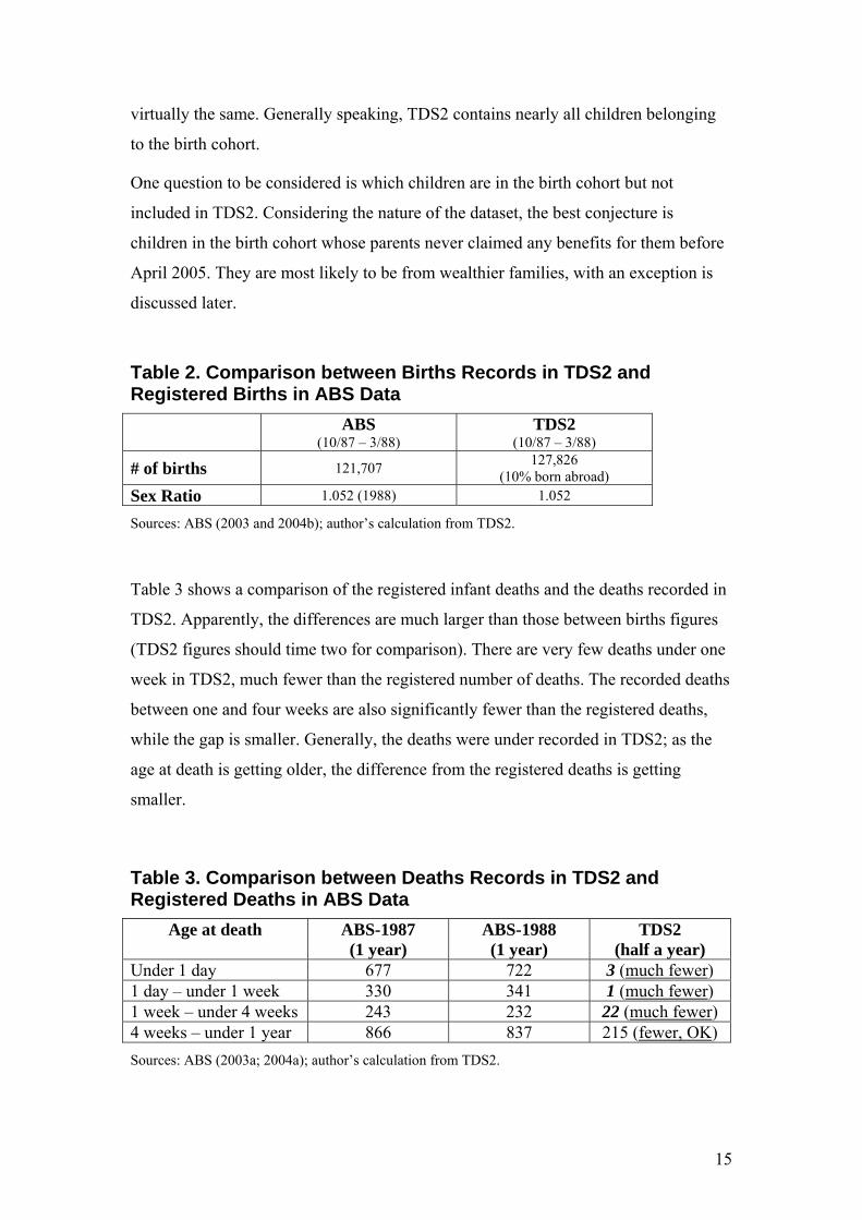
virtually the same. Generally speaking, TDS2 contains nearly all children belonging

to the birth cohort.

One question to be considered is which children are in the birth cohort but not

included in TDS2. Considering the nature of the dataset, the best conjecture is

children in the birth cohort whose parents never claimed any benefits for them before

April 2005. They are most likely to be from wealthier families, with an exception is

discussed later.

Table 2. Comparison between Births Records in TDS2 and Registered Births in ABS Data ABS

(10/87 – 3/88) TDS2

(10/87 – 3/88)

# of births 121,707 127,826 (10% born abroad)

Sex Ratio 1.052 (1988) 1.052

Sources: ABS (2003 and 2004b); author’s calculation from TDS2.

Table 3 shows a comparison of the registered infant deaths and the deaths recorded in

TDS2. Apparently, the differences are much larger than those between births figures

(TDS2 figures should time two for comparison). There are very few deaths under one

week in TDS2, much fewer than the registered number of deaths. The recorded deaths

between one and four weeks are also significantly fewer than the registered deaths,

while the gap is smaller. Generally, the deaths were under recorded in TDS2; as the

age at death is getting older, the difference from the registered deaths is getting

smaller.

Table 3. Comparison between Deaths Records in TDS2 and Registered Deaths in ABS Data

Age at death ABS-1987 (1 year)

ABS-1988 (1 year)

TDS2 (half a year)

Under 1 day 677 722 3 (much fewer) 1 day – under 1 week 330 341 1 (much fewer) 1 week – under 4 weeks 243 232 22 (much fewer) 4 weeks – under 1 year 866 837 215 (fewer, OK) Sources: ABS (2003a; 2004a); author’s calculation from TDS2.

15

Figure 3 shows the mortality of the primary children in TDS2 by age group. The

infant death rates of both boys and girls – around two per 1,000 live births – are

clearly smaller than those in ABS data – 9.8 and 7.6 per 1,000 live birth of boys and

girls, respectively, in 1988 (ABS 2004a). However, comparable ABS figures for other

age groups in TDS2 are difficult to find, because the deaths in TDS2 happened over

several years whereas ABS figures usually refer to a single year.

Figure 3. Mortality of Primary Children by Age

Mortality of Primary Children by Age

0

0.5

1

1.5

2

2.5

0 1~4 5~9 10~14 15~17

Age (years)

Deat

hs p

er 1

000

GirlsBoys

It is crucial for this research to understand the source of the differences between the

recorded number of deaths in the TDS2 and the ABS registered number of deaths.

An important question to ask is whose deaths were not recorded in TDS2?

Apparently, the deaths of children who were in the birth cohort but were not included

in TDS2 were not recorded. As mentioned above, children from wealthy families are

likely to be excluded from TDS2, but the exclusion of their deaths alone can hardly

explain the big differences, especially considering their small proportion in the birth

cohort and also their likely lower-than-average mortality risks. Another possibility

(and a better conjecture) is that children in the birth cohort who died within one or

two months were under-recorded in TDS2. These children usually had a serious

illness, which kept their parents busy with taking care of them, and therefore did not

16

have chance to claim benefits for them. Apart from their deaths, their births might not

be recorded in TDS2, either; in other words, TDS2 has no records of them at all.

This under-recording of deaths may not be random4, and because of the small number

of total deaths in TDS2, this is a more serious problem than the exclusion of children

from wealthy families. For instance, if children from disadvantaged families are

significantly more likely to die within one or two months, the analysis based on TDS2

death records will under-estimate the gap in mortality risk between disadvantaged and

other families. One solution for this issue is excluding all children who died within

two months. Similar robust tests have been undertaken using samples excluding

children who died within one or three months, and the key findings are qualitatively

the same. The following sections will give a more detailed discussion on this issue.

In addition, for children already included in TDS2, their deaths may also be under-

recorded. This happens when the children died after their parents left benefits and did

not return till the last recorded date in TDS2 (8 April 2005). This is a right-censoring

issue, and can be dealt with using duration models.

3.2 Parents5

In TDS2, 2,227 primary children do not have any parent identifies (IDs), so their

parents cannot be identified. For the other 125,599 primary children, 152,860 parents

are identified, and some of these parents once claimed benefits for more than one

primary child. Among the parents, the one who provided the longest care for a

primary child is referred to as the primary parent. Except for the 2227 children

without parent IDs, each primary child is associated with a primary parent. The

analysis in this paper is mainly based on the primary parents, and some duration

models use information of all parents.

Characteristics of the 125,599 primary parents and their correlation with mortality of

children are discussed in detail in Section 4. Briefly speaking, a vast majority of the

primary parents (more than 96%) are female6, two thirds were born in Australia, and

3.17 percent were identified as Indigenous. Surprisingly, although 41.6 percent of the

4 For example, births by people currently on benefits are likely to be reported sooner than births by people not on benefits. 5 In TDS2, parents refer to people who claimed FTB/FPA for the primary children. Therefore, they can be grandparents, older siblings or other guardians, and not necessarily actual parents of the children. 6 There are 61 parents with sex missing. Among them, 21 have individual IS records, and 18 have family IS records.

17

parents have individual income support (IS) records, only 40 percent have family IS

records in TDS2. This is due to another issue with TDS2: the family IS records were

left-censored (starting in 1993), whereas the individual IS records can go back to the

1960s. Therefore, in this research parental IS experience is mainly based on individual

IS records; however, preliminary analyses show that using family IS records leads to

similar results.

3.3 Issues and Solutions regarding TDS2 TDS2 has several outstanding advantages for the current research. First, it contains

nearly a whole birth cohort in the Australian population. Second, it contains detailed

benefit-related information of both primary children and their parents. Third, it is a

unit record data. Fourth, it is a longitudinal data. Fifth, variables in the dataset,

especially key benefit-relevant variables, are generally accurate. The data is not

subject to recall errors, which are common to survey data.

However, as an administrative data, TDS2 also has limitations, which should be

considered in the analysis.

First, it has a limited number of variables, and information of important factors

influencing mortality, such as neighbourhood information, is not available in the

dataset. As a result, unobserved heterogeneity is an issue.

To deal with this issue, Socio-Economic Indexes for Areas (SEIFA) disadvantage

index and Australian Standard Geographic Classification (ASGC) remoteness

classification7 are merged into the dataset by postcode.

Second, TDS2 only has records for customers when they are receiving benefits from

the Government. In other words, people who never receive benefits from the

Government are not included in the dataset, and no information is recorded when

people are off the benefit8.

People who have never claimed any benefit are thought to be mostly wealthy people.

As discussed above, they only account for a small proportion of the population of

interest, thus excluding them from the analysis is not a big issue. The concern

7 For details regarding the SEIFA index and ASGC remoteness classification, refer to the website of Australian Bureau of Statistics (ABS): www.abs.gov.au. 8 One exemption is that limited information of dependents, such as date of birth, date of death and sex, is provided by their guardians and also recorded in the dataset.

18

regarding that no information is recorded when people are off benefit is much bigger,

but can be easily tackled with duration models.

Third, not all deaths of children were recorded in TDS2. If the recording of deaths is

not random, the estimation based on TDS2 will be biased. As talked above, deaths

within two months after birth are likely to be under-recorded in TDS2 and also likely

to be non-random. One solution for this issue is to exclude these deaths from the

analysis and test the robustness of key findings.

Fourth, some variables, such as family income and SEIFA index, have many missing

values. In this research, if the missing values account for a fairly large proportion of

the total observations, and/or the mortality of the missing observations is significantly

different from the sample mean, a separate category for the missing values is created.

This list does not cover all the issues regarding the dataset (some will be discussed

later); even for the listed issues, the solutions talked above are not totally satisfactory.

Therefore, various tests have been undertaken to check the robustness of key findings.

More detailed discussions can be found in later sections.

3.4 Sample For most of the analyses in this research, three groups of primary children were

excluded. First, children whose parent IDs are missing were excluded, because the

correlation between mortality of children and parental disadvantage cannot be

analysed without information of the parents.

Second, children who were born abroad were also excluded. Among all premature

deaths, infant death rate (especially neonatal mortality) is the highest; only a small

proportion of foreign born children were likely to be in Australia as infants.

Therefore, the mortality of foreign born children is likely to be underestimated with

TDS2.

Third, for reasons discussed above, children who died within two months after birth

were excluded. For robust tests, analyses for children who survived to three months

and for all primary children in TDS2 were also undertaken and the key findings are

generally consistent.

In the following sections, if not otherwise specified, the sample of primary children

used for this research is restricted to the primary children whose parents can be

19

identified and who were born in Australia and did not die within two months after

birth. This consists of 119,013 primary children, with 51.3 percent being boys. The

mortality rates of the whole sample, boys and girls are 0.49 percent, 0.57 percent and

0.41 percent, respectively.

Each primary child is associated with a primary parent in the sample. Characteristics

of primary parents and their correlation with mortality of children are discussed in

detail in the next section.

20

4. Descriptive Analysis This section undertakes the descriptive analysis. Correlations between mortality of

children and observed characteristics of children and their primary parents were

investigated with direct tabulation and figures. Particular attention is given to the

correlation between mortality of children and several indicators of parental

disadvantage, including Indigenous status, teenage motherhood, non-birth-parent,

disability, low income, long income support duration, and living in a remote or socio-

economically disadvantaged area.

In order to see the significance of various influencing factors, a demographic concept

– excess death – is used. Excess death is the difference between the observed number

of deaths in a group and the number of deaths that would have occurred in that group

if it had the same mortality rate as a reference group. In this section, the least

disadvantaged group is usually used as reference. The estimated excess deaths are

presented in Table 4.

4.1 Indigenous Status

The Indigenous status in TDS2 is based on self identification. In addition, if a

customer chose to receive Family Tax Benefit (FTB) through Australian Tax Office in

a lump sum at the end of a financial year, this variable was not recorded in the

Centrelink system. Presumably, this is not commonly the case for Indigenous people,

and is more likely to happen among less disadvantaged Indigenous people.

Nonetheless, Indigenous people were not fully identified in TDS2, and this is also a

common issue for most Australian datasets.

As shown in Table 4, the mortality rate of children of non-Indigenous people is 0.47

percent, whereas the rate for Indigenous children9 is 0.89 percent. In other words, the

mortality risk of Indigenous children is 1.89 times as large as that of non-Indigenous

children.

9 In TDS2, some parents of the primary children who are identified as Indigenous are not Indigenous themselves; in the meantime, there are also some children of Indigenous people not being identified as Indigenous. In this paper, for simplicity of expression, Indigenous children refer to children of Indigenous people.

21

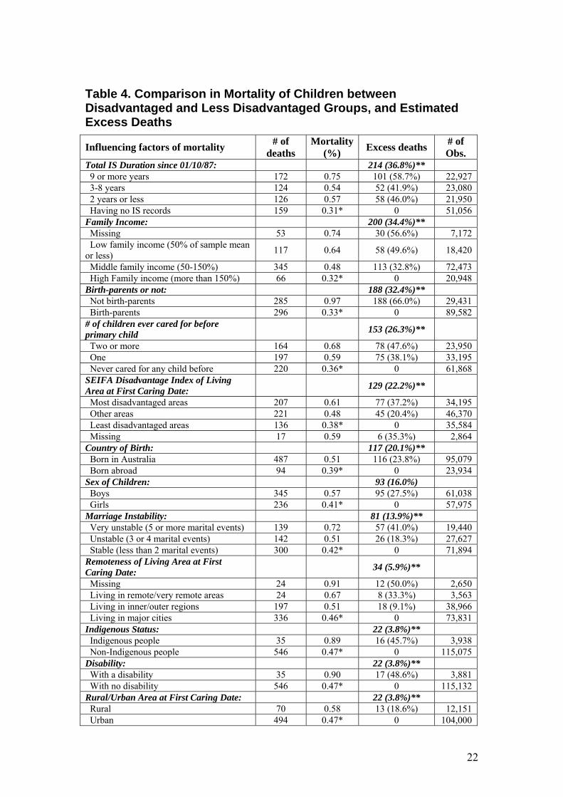
Table 4. Comparison in Mortality of Children between Disadvantaged and Less Disadvantaged Groups, and Estimated Excess Deaths

Influencing factors of mortality # of deaths

Mortality (%) Excess deaths # of

Obs. Total IS Duration since 01/10/87: 214 (36.8%)** 9 or more years 172 0.75 101 (58.7%) 22,927 3-8 years 124 0.54 52 (41.9%) 23,080 2 years or less 126 0.57 58 (46.0%) 21,950 Having no IS records 159 0.31* 0 51,056 Family Income: 200 (34.4%)** Missing 53 0.74 30 (56.6%) 7,172 Low family income (50% of sample mean or less) 117 0.64 58 (49.6%) 18,420

Middle family income (50-150%) 345 0.48 113 (32.8%) 72,473 High Family income (more than 150%) 66 0.32* 0 20,948 Birth-parents or not: 188 (32.4%)** Not birth-parents 285 0.97 188 (66.0%) 29,431 Birth-parents 296 0.33* 0 89,582 # of children ever cared for before primary child 153 (26.3%)**

Two or more 164 0.68 78 (47.6%) 23,950 One 197 0.59 75 (38.1%) 33,195 Never cared for any child before 220 0.36* 0 61,868 SEIFA Disadvantage Index of Living Area at First Caring Date: 129 (22.2%)**

Most disadvantaged areas 207 0.61 77 (37.2%) 34,195 Other areas 221 0.48 45 (20.4%) 46,370 Least disadvantaged areas 136 0.38* 0 35,584 Missing 17 0.59 6 (35.3%) 2,864 Country of Birth: 117 (20.1%)** Born in Australia 487 0.51 116 (23.8%) 95,079 Born abroad 94 0.39* 0 23,934 Sex of Children: 93 (16.0%) Boys 345 0.57 95 (27.5%) 61,038 Girls 236 0.41* 0 57,975 Marriage Instability: 81 (13.9%)** Very unstable (5 or more marital events) 139 0.72 57 (41.0%) 19,440 Unstable (3 or 4 marital events) 142 0.51 26 (18.3%) 27,627 Stable (less than 2 marital events) 300 0.42* 0 71,894 Remoteness of Living Area at First Caring Date: 34 (5.9%)**

Missing 24 0.91 12 (50.0%) 2,650 Living in remote/very remote areas 24 0.67 8 (33.3%) 3,563 Living in inner/outer regions 197 0.51 18 (9.1%) 38,966 Living in major cities 336 0.46* 0 73,831 Indigenous Status: 22 (3.8%)** Indigenous people 35 0.89 16 (45.7%) 3,938 Non-Indigenous people 546 0.47* 0 115,075 Disability: 22 (3.8%)** With a disability 35 0.90 17 (48.6%) 3,881 With no disability 546 0.47* 0 115,132 Rural/Urban Area at First Caring Date: 22 (3.8%)** Rural 70 0.58 13 (18.6%) 12,151 Urban 494 0.47* 0 104,000

22

Teenage motherhood: 10 (1.7%)** Teenage mothers 42 0.74 15 (35.7%) 5,663 Non-teenage mothers 539 0.48* 0 113,350 Homeownership at First Caring Date: 10 (1.7%)** Living in government houses 78 0.86 34 (43.6%) 9,065 Homeowners 246 0.48* 0 51,485 Missing 65 0.30 -41 (-63.1%) 22,018 Total 581 0.49 119,013

Notes: * Mortality rates used for calculating excess deaths. ** Estimated excess deaths for the whole sample. Figures in parentheses are percentages of deaths which could be reduced if mortality rates of the reference groups were applied. The factors are ordered by estimated excess deaths for the whole sample. The differences between the estimated excess deaths for the whole sample and the sum of estimated excess deaths of sub-groups are due to rounding of figures in calculation.

The estimated number of excess deaths for the whole sample is 22. This means if the

death rate of the whole sample could be reduced to the rate of non-Indigenous

children, the total number of deaths would be 22 fewer than observed.

Since Indigenous children only account for a small proportion of the sample,

narrowing the gap does not make a big difference for the whole sample – the number

of excess deaths is only 3.8 percent of the total observed number of deaths. However,

the effect on the most disadvantaged group – Indigenous children – is very

significant; the number of deaths of Indigenous children could have been reduced by

nearly half if they had the same death rate as non-Indigenous children.

4.2 Country of Birth As mentioned in the last section, all primary children who were born abroad were

excluded from the sample10, while children whose parents were born abroad were

included. In the sample, about 20 percent of primary parents were born abroad11.

As shown in Table 4, the mortality of children is much lower for immigrants than for

Australian born people. The estimated number of excess deaths is 117, accounting for

one fifth of the total deaths of children in the sample. Why is the mortality of children

necessarily lower for immigrants than the Australian born people? Several reasons are

discussed in Section 6 – Summary and Discussion.

10 It should be noted that not all children who were born abroad were excluded because country of birth was unknown for at least half of the primary children (non-customers). In general, children of immigrants are more likely to be born abroad than other children; this may also partly explain the lower mortality of children for immigrants in the sample. 11 Among all primary parents in the clean sample, approximately 3% primary parents were born in six main English-speaking countries – US, UK, Canada, New Zealand, Ireland, and South Africa – and 17% were born in other countries. The mortality rates of children for parents born in the main English-speaking countries and parents born in other countries are 0.2% and 0.43%, respectively.

23

4.3 Disability In the current study, disability is used as a dummy variable, and is defined as being

eligible for the Disability Support Pension (DSP). In the sample, there are

approximately 3.3 percent of children whose primary parents have a disability.

Their mortality risk is nearly two times that of other children. Again, because of their

small proportion in the sample, reducing their mortality to the level of other children

has little effect on the whole sample but the impact is very significant for this

disadvantaged group – the number of deaths could have been reduced to half of the

observed level.

4.4 Teenage Motherhood In the current study, a teenage mother refers to a woman who became the primary

carer of a primary child as a teenager; in the sample 5,663 women (4.8%) fall into this

category12.

As shown in Table 4, the mortality of children primarily cared for by teenage mothers

is also significantly higher than that of others (0.74% in comparison to 0.48%). The

estimated number of excess deaths is small for the whole sample but fairly large for

the children of teenage mothers.

In addition, the mortality of children generally decreases with the aging of primary

parents up to 35, and it slightly goes up when the primary parents are older than 35

years.

4.5 Birth-parent In the TDS2 there is no information about the actual relationship between a ‘primary

parent’ and a ‘primary child’, but in most cases the primary parents would most likely

be the natural parents. Since there is evidence for differences between birth-parents

and non-birth-parents regarding caring for and the outcomes of children13, a variable

of birth-parent is derived to see this difference for Australian children.

In this paper a birth-parent is defined as a primary carer who started taking care of a

primary child from the time of birth14. Although a birth-parent defined in such a way

12 According to ABS (1994), in 1988, 5.6 percent babies were born to teenage mothers. 13 For instance, Case and Paxon (2001) show that stepmothers are not a good substitute of mothers. 14 Redefining a birth-parent as a primary carer who started taking care of a primary child within 6 months after birth makes little difference on the main findings.

24

is likely to be the actual birth-parent, in reality it does not cover all actual birth-

parents because the caring date in TDS2 is based on the date of claiming benefits for a

primary child rather than the actual start of care date. Therefore, an actual birth-parent

of a child can be classified as a non-birth-parent here if her first recorded caring date

in TDS2 is different from the date of birth of the child.

As shown in Table 4, the mortality of children is nearly three times as large for non-

birth-parents as for birth-parents. However, for the above mentioned reasons, to

simply attribute the observed differences in mortality of children to the differences

between natural birth-parents and non-birth-parents in Australia should be done so

with caution.

4.6 Number of Children before a Primary Child In TDS2 there is a variable of the total number of FTB/FPA children associated with a

parent or spouse. However, due to the replacement effect15, the value of this variable

may be affected by the death of a primary child (i.e., potentially endogenous). To

avoid this endogeneity problem, a new variable consisting of number of children ever

cared for before the primary child (equivalent to the birth order of the primary child in

most cases) is generated and used in the analysis.

As shown in Table 4, more than half of the primary children were the first child of

their primary parents; their mortality is only 0.36 percent, in comparison to 0.59

percent for the second children, and 0.68 percent for the third and later children.

The estimated excess deaths are fairly significant. If the mortality rate of the whole

sample was the same as that of those who are the first child of their primary parents,

the total number of deaths could have been reduced by more than one quarter. The

effects are even larger for the sub-groups of the second or later children.

4.7 Income Support History Due to the nature of the data, all parents in TDS2 had once received family payments

such as family tax benefits (FTB), but not all of them received income support (43%

have no IS records). Compared to those who only received non income support family

payments, families on income support are more disadvantaged because their main

source of income is the Government benefit. Therefore, the incidence and duration of 15 Families with high mortality of children tend to have more children than their ideal number in order to reach the desired number of surviving children.

25

income support may be a good indicator of family economic disadvantage, especially

long-term disadvantage.

In TDS2, both family income support history and individual income support history

are recorded. However, family income support records are left truncated at 1993,

whereas individual records can be traced back to the 1960s. In addition, there are

some inconsistent cases in the family income support records and also inconsistent

cases between family and individual records. Therefore, individual records are mostly

chosen to derive the variables of income support incidence and duration, while family

records are used for robust tests; the findings are generally consistent.

There are different ways to generate the variables of income support incidence and

duration from different time periods of TDS2 records, and these variables have

different implications.

First, they can be derived from total income support records in TDS2. This method is

the most straightforward, and the variables indicate the long-term economic

disadvantage of the primary parents. However, one issue with this method is that

older people are more likely to have an income support spell and also have longer

income support duration simply because they are older and thus have been exposed to

the system longer.

Second, the variables can be generated from records up to the birth (or the first caring

date) of a primary child. Theoretically, the variables derived in this method are least

likely to be affected by the birth/care of the primary child, but the problem is that they

may not reflect the actual living environment of the child and the issue for the first

method still exists here. In addition, a practical problem for this method is that few

primary parents had income support records before the birth (or the first caring date)

of a primary child.

Third, the variables can be created from the records up to the last caring date, or the

records between the first and the last caring dates. In this way the variables can better

reflect the actual family economic situation of the child, but they are also correlated

with the surviving time of the child, which is significantly correlated with the

mortality risk of children. These two correlations may bias the estimated correlation

between IS duration and mortality of children. One solution is using the proportion of

time on income support while caring for the child instead of the duration variable.

26

Fourth, a fixed time window (1 October 1987 to 8 April 200516) can be used for all

sample members. In this way, the variable of total IS duration is equivalent to the

proportion variable because the denominator is the same for all members. In the

meantime, a dummy variable is also created to indicate whether a primary parent had

income support records before 1 October 1987.

All these methods have their advantages and disadvantages where none of them are

perfect, however, the second and the third seem to be the most problematic. In this

paper, the fourth method is mostly used, because it is relatively better in reflecting the

family (long-term) economic disadvantage of primary children between age zero and

age 17. The first method generally leads to very similar results to the fourth. For a

comparison between different measures of IS duration, see Table A1 in The

Appendix.

As shown in Table 4, mortality is the lowest for children whose parents have no IS

records since 1987 (0.31%), whereas it is the highest for those whose parents had

been on IS for nine years or longer between 1987 and 2005 (0.75%). The estimated

number of excess deaths for the whole sample is 214, accounting for 36.8 percent of

the total number of deaths. The effect is the largest among all influencing factors,

suggesting that total IS duration is a key indicator of parental disadvantage with

regard to mortality of children.

4.8 Family Income Both family income and individual income are recorded in TDS2. Family income is

predominantly used in this research, and individual income is used for robust tests; the

findings are qualitatively the same.

There are several issues about income variables in TDS2. First, incomes are only

available for the years between 1991 and 2004. Second, there are many missing

values (for more than 6% of the sample). Third, even after the deflation with

Consumer Price Index (CPI), there is still an increasing trend (see Figure 4).

To tackle these issues, the following approach is applied: firstly, the sample mean of

family income is calculated for each year between 1991 and 2004; secondly, family

16 The current version of TDS2 was extracted on 8 April 2005. Later on in this paper, both terms of time since 1987 and time between 1987 and 2005 refer to the same period of time, i.e., 1 October 1987 and 8 April 2005.

27

income is divided by the sample mean in a given year to generate a measure of

relative position of family income in the sample; thirdly, the average of relative

family income is calculated over all recorded years; finally, the average relative

family income is classified into four categories17: (1) low family income (50% of

sample mean or less), (2) middle family income (50-150% of sample mean), (3) high

family income (more than 150% of sample mean), and (4) missing.

Figure 4. Trend in Real Income in TDS2

0

5000

10000

15000

20000

25000

30000

35000

Aver

age

Inco

me

(in 1

989$

)

19911993

19951997

19992001

2003

Year

Trend in Income

Family Income Individual Income

As shown in Table 4, the mortality of children generally decreases with relative

family income: the mortality is 0.32 percent, 0.48 percent, and 0.64 percent for

children from high income, middle income and low income families, respectively.

Children whose parental family income is missing appear to have the highest

mortality, which indicates the missing values in family income are not random.

Therefore, the missing values in family income are put into a separated category

rather than dropped from the analysis in this research.

17 Continuous variable of family income and its quadratic form are also used in some preliminary analyses, and the coefficients of other variables are hardly affected.

28

The estimated number of excess deaths is also very large (the second largest among

all variables in Table 4), accounting for 34.4 percent of total deaths of the primary

children in the sample. Once again, this suggests a significant role of economic

factors in the mortality of children.

4.9 Marriage Instability Any changes in marital status while on benefits are required to be reported to

Centrelink. There is a problem in TDS2 about marital status; that is, the vast majority

of people in TDS2 had their first marital status recorded as SINGLE, and a vast

majority of the dates recorded for the first marital status were the dates of BIRTH. As

a result, the first record on marital status is useless. Another difficulty is that marital

status can be correlated with age and also change over time.

Therefore, in this research, a variable of marriage instability is used instead. This is

derived from the number of recorded marital events in TDS2: (1) stable, if having

only one or two marital events; (2) unstable, if having three or four marital events;

and (3) very unstable, if having more than five marital events.

However, one issue remains; that is, if a person stays on benefit longer, she is likely to

have more marital events recorded. Therefore, this variable is just a rough measure of

marriage instability.

4.10 SEIFA Disadvantage Index There is no relevant information of location and neighbourhood in TDS2 except

postcode. To tackle this problem, in this research, Socio-Economic Indexes for Areas

(SEIFA) Index of Disadvantage and the remoteness classification of Australian

Bureau of Statistics (ABS)18 are merged into TDS2 by postcode.

SEIFA Index of Disadvantage provides rankings for a wide range of areas. It is

particular useful for this research because it focuses on low income earners, relatively

lower educational attainment, and high unemployment, which reflect several key

characteristics of socio-economically disadvantaged areas.

Since people change residential addresses from time to time, SEIFA index is merged

into TDS2 in several ways: (1) based on the first caring dates; (2) based on the last

18 For more details of SEIFA index and remoteness classifications, refer to ABS website at www.abs.gov.au.

29

caring dates; (3) for all relevant dates of interest (for survival analysis). These

different ways lead to generally consistent results.

The SEIFA Index of Disadvantage is in continuous form, and the larger the index, the

less the relative disadvantage. In this paper the areas are classified into three

categories based on the index: (1) most disadvantaged areas (the first thirty percentiles

of SEIFA Index of Disadvantage); (2) least disadvantaged areas (the last thirty

percentiles of the index); (3) other areas (the middle forty percentiles of the index). In

addition, the SEIFA index is not available for 2864 pairs of children and parents,

therefore, they are put into a separate category – Missing.

As shown in Table 4, the mortality is significantly lower for children living in the

socio-economically least disadvantaged areas (0.38%) than those living in the most

disadvantaged areas (0.61%). The estimated number of excess deaths account for

more than one fifth of the total number of deaths of children in the sample. In

addition, the areas with missing values of SEIFA index also have high mortality of

children (0.59%), suggesting that the missing values of SEIFA index are not randomly

distributed, and they are more likely to happen among disadvantaged areas.

4.11 Remoteness Remoteness information comes from the Australian Standard Geographic

Classification (ASGC) Remoteness Areas classification of ABS. The classification

puts populated localities into six classes: major cities, inner regional, outer regional,

remote, very remote, and migratory areas. This information is also merged into TDS2

by postcode.

In the sample, 62 percent lived in major cities at the first caring date, 32.7 percent

lived in inner/outer regions, only three percent lived in remote/very remote areas and

the other 2.2 percent or so have remoteness classification unknown.

As shown in Table 4, remoteness is also found to be positively correlatively with

mortality of children. The mortality is 0.46 percent for children in major cities, 0.51

percent for those in inner/outer regions, 0.67 percent for those in remote/very remote

areas, and the areas with remoteness unknown have the highest mortality of children –

0.91 percent.

30

The estimated number of excess deaths is not large for the sample, but for the children

living in remote/very remote areas, the number accounts for one third of total

observed deaths.

Since Indigenous Australians make up a substantial proportion of rural and

(particularly) remote area populations, it is often difficult to tell whether the

differences come from the actual location or Indigenous status. From Figure 5 it

seems that high mortality of children in remote/very remote areas is mainly driven by

high mortality of Indigenous children. Another point to note is that mortality rates of

children are extremely high in areas with remoteness missing, indicating that these

areas with remoteness missing are likely to be in remote/very remote areas.

Figure 5. Mortality of Children by Remoteness and Indigenous Status

0

0.5

1

1.5

2

2.5

3

3.5

Major citie

s

Inner regions

Outer regions

Remote areas

Very remote

Missing

Mor

talit

y (%

)

Whole sample

Non-Indigenous

Indigenous

In addition, the rural or urban areas and states of residence can also be identified from

postcodes, but they are not given much emphasis because preliminary multivariate

analyses show that they are rarely significant. In the sample, only 10 percent lived in

rural areas, and more than 92 percent lived in New South Wales, Victoria,

Queensland, Western Australia and South Australia. The proportions are

approximately the same at the first caring dates as at the last caring dates. Generally,

31

the mortality of children is higher in rural areas than in urban areas, and it is also

higher in Northern Territory than in other states, whereas the Australian Capital

Territory has the lowest mortality of children.

4.12 Sex of Children As mentioned in Section 3, there is very little information available for all primary

children in TDS2, apart from sex, date of birth and date of death.

First, the mortality is compared by gender of primary children. As expected, the

mortality of boys (0.57%) is higher than that of girls (0.41%).

Second, the mortality is also compared by month of birth. The primary children

belong to a half year birth cohort, thus there is little difference in age. However, it is

interesting to examine whether different birth months are associated with different

mortality rates which could be due to season related factors, such as weather and

holiday arrangements of parents and health services. Direct tabulation shows that

mortality is the lowest for children born in December (0.44 %), and is the highest for

children born in November and January (0.52%). However, birth months are generally

insignificant in multivariate analyses and thus mostly excluded.

In Table 4 the influencing factors are ordered by the estimated excess deaths for the

whole sample. These factors can be grouped into several broad categories: (1)

economic factors (IS duration and family income), (2) care related factors (number of

children before the primary child, birth-parent, disability, teenage motherhood and

marriage instability), (3) family background (Indigenous status and country of birth),

(4) location/neighbourhood factors (SEIFA index, remoteness, rural/urban and

state/territory of residence), and (5) children’s own characteristics (sex and birth

months).

Generally, the descriptive analyses show that disadvantaged groups in the different

aspects have higher mortality of children than less disadvantaged groups, where

economic and care related disadvantages seem to have the most significant effects.

4.13 Correlation between the Influencing Factors The factors influencing mortality of children are not independent from each other.

Table 5 shows the correlation matrix of the main influencing factors. Some factors are

32

highly correlated; for instance, total IS duration is highly correlated with relative

family income, marriage instability, teenage motherhood and disability.

The table also shows that Indigenous status is highly correlated with remoteness,

suggesting that Indigenous people are likely to live in remote/very remote areas. They

are also more likely to have other disadvantaged characteristics, such as longer IS

duration, lower family income, higher marriage instability, being a teenage mother

and living in socio-economically disadvantaged areas. All these disadvantages may

have contributed to the higher mortality of Indigenous children.

Teenage mothers not only are likely to have longer IS duration and lower family

income, but also tend to have more marital events recorded in TDS2 (i.e., their

marriage status is less stable). In addition, considering their age, it is not surprising to

find that they are less likely to have had any children before the primary child.

Birth-parents are highly correlated with the number of children ever cared for before.

This may be because of the definition of birth-parent; that is, primary carers who

started to ‘take care of’ – claiming family payments for – a primary child from the

time of birth. If a parent had children (likely to young) before the primary child, she

was more likely to be on benefits at the birth of the child, and thus had a higher

probability of claiming family payments for the child from the birth time.

People with a disability tend to have longer IS duration and lower family income, be

living in remote/very remote areas, and have unstable marriage status. Marriage is

very likely to be unstable for people with longer IS duration and lower family income,

or living in socio-economically disadvantaged areas. Several location and

neighbourhood variables – remoteness, SEIFA index and rural/urban – are also highly

correlated, partly due to the fact that they are all derived from postcode.

33

Table 5. Correlation between Factors Influencing Mortality of Children

Death

of child

Indigenous Teenage mothers

# of children before

Disabled Birth-parent Marriage

instabilityIS

duration

Relative family income

Remoteness SEIFA index

Death of child 1.0000

Indigenous 0.0059 1. 0000

Teenage mothers 0.0094 0.1131 1.0000

# of children before 0.0174 0.0682 -0.1376 1.0000

Disabled 0.0093 0.0381 0.0040 0.0491 1.0000

Birth-parent -0.0426 -0.0184 0.0885 0.2815 -0.0009 1.0000

Marriage instability 0.0129 0.1346 0.1808 0.0157 0.1099 0.0002 1.0000

IS duration 0.0182 0.1758 0.2047 0.0648 0.2045 0.0326 0.5648 1.0000

Relative family income -0.0123 -0.1411 -0.1309 -0.0756 -0.1414 -0.0236 -0.3344 -0.5892 1.0000

Remoteness 0.0049 0.2392 0.0539 0.0697 0.1116 0.0272 0.0652 0.0695 -0.0745 1.0000

SEIFA index -0.0106 -0.1101 -0.0754 -0.0377 -0.0445 -0.0287 -0.1077 -0.1858 0.1621 -0.2199 1.0000

Rural 0.0032 0.0826 0.0128 0.0544 0.0027 0.0333 0.0141 0.0257 -0.0629 0.4008 0.0105

Notes: Total observations = 108781; Missing values are excluded.

34

5. Econometric Analysis

5.1 Probability of Having a Primary Child Who Died

In the last section, mortality is found to be different for children from different family

backgrounds, and, in particular, economic and care related factors make significant

differences. This section estimates the effects of these factors on the mortality risk of

children with a logistic model.

For convenience of analysis, the influencing factors are grouped into five categories

as discussed in the last section: (1) family background; (2) care related factors; (3)

economic factors; (4) location/neighbourhood factors; and (5) children’s own

characteristics.

The model takes the following general form:

Y* = β0 + β1 X1 + β2 X2 + β3 X3 + β4 X4 + β5 X5 + ε (1)

where Y* is a latent variable referring to the health conditions of children, X1 is an

array of family background variables, X2 is an array of variables affecting care of

children, X3 is an array of economic variables, X4 is an array of

location/neighbourhood variables, X5 is an array of variables about characteristics of

children, β0 is a constant term, β1 – β5 are vectors of coefficients for variables in the

five categories, and ε is a term of random error.

If the health condition of a child is worse than a certain level, it will lead to death of

the child. That is

{otherwise

YifY

,00*,1 >

= (2)

An estimation strategy that was applied consists of starting with a group of factors in

one category (baseline model), then including more explanatory variables of other

categories in stage (extension models) to check the sensitivity of the coefficients of

the factors in the baseline model.

35

5.1.1 Family Background

There are two variables in this category: Indigenous status and county of birth. These

may be associated with certain family values, culture and living style.

As shown in Table 6, in the Baseline Model, when no other variables are included

except country of birth, Indigenous status is very significant, and the probability of

premature death of an Indigenous child is about 80 percent higher than a non-

Indigenous child. However, when more explanatory variables are included in the

model, Indigenous status becomes insignificant. This suggests that the higher

mortality of Indigenous children may be explained mainly by their parental

disadvantage in other aspects, such socio-economic disadvantage, rather than their

parental Indigenous status alone.

Country of birth shows significant effects on the mortality of children, and

immigrants generally have a lower mortality of children than people born in Australia.

In particular, the mortality risk of children is 60-70 percent lower for people born in

main English-speaking countries than for Australia born people.

Table 6. Estimated Effects of Family Background Factors on Mortality Risk of Children (odd ratios) Variables Baseline

Model Extension 1 Extension 2 Extension 3 Full Model

Indigenous 1.80 (3.35) ***

0.99 (0.05) 1.00 (0.02) 0.88 (0.64) 0.88 (0.64)

Country of birth: Australia Reference Reference Reference Reference Reference Main English-speaking countries

0.40 (2.43) **

0.29 (3.23) ***

0.29 (3.24) ***

0.28 (3.28) ***

0.28 (3.28) ***

Other countries 0.86 (1.30) 0.72 (2.74) ***

0.72 (2.77) ***

0.65 (3.38) ***

0.65 (3.38) ***

Notes: * Significant at 10% level, ** Significant at 5% level, *** Significant at 1% level. Absolute values of z-statics in parentheses (standard errors adjusted for clustering on parent ID). In Extension 1, five care related variables (number of children cared before primary child, teenage motherhood, disability, birth-parent, marriage instability) are also included. In Extension 2, a dummy variable for boy is also included. In Extension 3, three economic variables (having IS before 1987, total IS duration since 1987, and relative family income) are also included. In the Full Model, two location/neighbourhood variables (SEIFA index and remoteness) are also included.

36

5.1.2 Care Related Factors

Several observed factors in TDS2 may directly affect care of children, including

teenage motherhood, number of children cared for before the primary child, disability,

birth-parent, and marriage instability.

Being taken care of by a teenage mother increases the probability of death. As shown

in Table 7, the mortality risk of children whose primary carers were teenage mothers

at the first caring date is approximately three times as high as that of other children.

The effect hardly changes when more variables are included in the model.

Number of children ever cared for before also shows very significant effects on the

mortality risk of children. If a parent had one child before a primary child, the

probability of death of the primary child tends to be 2.62-2.84 times higher than if she

had no child before; if she had two children before the primary child, the mortality

risk of the primary child is even higher (3.3-3.64 times). However, if she had three or

more children before the primary child, the mortality risk starts to decrease a little. In

particular, if she had four or more children before the primary child, the mortality risk

is approximately 2.1-2.4 times as high as if she had no other child before, which is

lower than if she had fewer (1-3) children before the primary child.

The coefficient of the birth-parent variable is very significant and also very stable

with the inclusion of extra explanatory variables. Generally, the mortality risk of

children being taken care of by their birth-parents is only 84 percent lower than that of

other children.

Disability of parents also increases the mortality risk of children. The risk is about 45

percent higher if primary parents have a disability than otherwise. However, when

economic factors (IS duration and family income) are controlled for, the effect

becomes insignificant.

Similarly, instability of marriage is also associated with higher mortality of children.

The probability of death is about 40 percent higher for a child whose parent’s

marriage is very unstable – having five or more marital events in TDS2 – than for a

child whose parent’s marriage is stable – only having one or two marital events.

Again, due to the high correlation between marriage instability and economic factors,

the coefficient of this variable is insignificant in Extension 3 and the Full Model,

where income support duration and family income are included.

37

Table 7. Estimated Effects of Care Related Factors on Mortality Risk of Children (odd ratios) Variables Baseline

Model Extension 1 Extension 2 Extension 3 Full Model

Teenage motherhood

3.26 (6.70) ***

3.13 (6.39) ***

3.14 (6.39) ***

2.82 (5.74) ***

2.77 (5.64) ***

# of children before the primary child:

No child Reference Reference Reference Reference Reference 1 child 3.84 (10.71)

*** 3.73 (10.44) ***

3.75 (10.46) ***

3.63 (10.24) ***

3.62 (10.22) ***

2 children 4.64 (10.49) ***

4.51 (10.25) ***

4.51 (10.25) ***

4.31 (9.98) ***

4.30 (9.94) ***

3 children 4.10 (7.54) ***

3.97 (7.30) ***

3.98 (7.32) ***

3.70 (6.89) ***

3.65 (6.82) ***

4 or more children

2.38 (3.16) ***

2.33 (3.00) ***

2.34 (3.02) ***

2.12 (2.65) ***

2.10 (2.61) ***

Disability 1.45 (2.06) **

1.44 (2.00) **

1.45 (2.02) **

1.23 (1.10) 1.22 (1.06)

Birth-parent 0.17 (15.54) ***

0.16 (15.65) ***

0.16 (15.64) ***

0.16 (15.42) ***

0.16 (15.42) ***

Marriage instability:

Stable Reference Reference Reference Reference Reference Unstable 1.11 (0.99) 1.11 (1.02) 1.11 (1.00) 0.85 (1.46) 0.85 (1.42) Very unstable 1.41 (3.16)

*** 1.40 (3.06) ***

1.39 (3.04) ***

1.01 (0.08) 1.01 (0.10)

Notes: * Significant at 10% level, ** Significant at 5% level, *** Significant at 1% level. Absolute values of z-statics in parentheses (standard errors adjusted for clustering on parent ID). In Extension 1, two family background variables (Indigenous status and country of birth) are included. In Extension 2, a dummy variable for boy is also included. In Extension 3, three economic variables (having IS before 1987, total IS duration since 1987, and relative family income) are also included. In the Full Model, two location/neighbourhood variables (SEIFA index and remoteness) are also included.

5.1.3 Economic Factors

Three variables for economic factors are included in the model: total IS duration since

1987, having IS records before 1987 and relative family income. Both long IS

duration since 1987 and low family income are indicators of economic disadvantage,

and having IS records before 1987 indicates being even more disadvantaged given the

other factors are the same.

As shown in Table 8, primary parents having been on income support since 1987

(when the primary children were about to be born) generally have significantly higher

mortality risks of their children. However, interestingly, the mortality risk does not

monotonically increase with total IS duration; instead, the correlation shows a rather

38

complex pattern. Among parents with IS records since 1987, those with total

durations of between three and five years have the lowest mortality risk of children

(though still 47-55% higher than those without any IS records).

The effect of family income is generally insignificant, due to its high correlation with

IS duration. If IS duration is not controlled for, as expected, parents with higher

family income have significantly lower mortality of children.

Having IS records before 1987 also tends to increase the mortality risk of children,

but the effect is generally insignificant.

A comparison with other measures of IS history is shown in Table A2 in the

Appendix.

Table 8. Estimated Effects of Economic Factors on Mortality Risk of Children (odd ratios) Variables Baseline

Model Extension 1 Extension 2 Extension 3 Full Model

Having IS before 1987

1.49 (1.92) * 1.47 (1.83) * 1.16 (0.69) 1.16 (0.48) 1.15 (0.65)

Total IS duration since 1987:

No records Reference Reference Reference Reference Reference Less than 1 year 1.71 (3.39)

*** 1.73 (3.46) ***

1.72 (3.39) ***

1.72 (3.40) ***

1.69 (3.28) ***

1-2 years 1.89 (4.22) ***

1.93 (4.30) ***

1.87 (3.94) ***

1.87 (3.92) ***

1.83 (3.78) ***

3-5 years 1.55 (2.78) ***

1.55 (2.77) ***

1.51 (2.43) **

1.51 (2.45) **

1.47 (2.29) **

6-8 years 1.78 (3.64) ***

1.76 (3.55) ***

1.67 (3.00) ***

1.68 (3.02) ***

1.64 (2.85) ***

9-11 years 2.39 (6.02) ***

2.33 (5.76) ***

2.32 (5.03) ***

2.34 (5.04) ***

2.22 (4.72) ***

12 or more years 1.86 (3.56) ***

1.77 (3.25) ***

1.87 (3.28) ***

1.87 (3.30) ***

1.78 (3.01) ***

Family income: Low Reference Reference Reference Reference Reference Middle 1.00 (0.00) 0.99 (0.10) 1.18 (1.31) 1.18 (1.33) 1.19 (1.37) High 0.89 (0.64) 0.87 (0.76) 0.97 (0.19) 0.97 (0.18) 0.98 (0.11) Missing 1.28 (1.48) 1.32 (1.66) * 1.12 (0.66) 1.13 (0.69) 1.12 (0.65)

Notes: * Significant at 10% level, ** Significant at 5% level, *** Significant at 1% level. Absolute values of z-statics in parentheses (standard errors adjusted for clustering on parent ID). In Extension 1, two family background variables (Indigenous status and country of birth) are included. In Extension 2, five care related variables (number of children cared before primary child, teenage motherhood, disability, birth-parent, marriage instability) are also included. In Extension 3, a dummy variable for boy is also included. In the Full Model, two location/neighbourhood variables (SEIFA index and remoteness) are also included.

39

5.1.4 Location/Neighbourhood Factors There are four location/neighbourhood variables derived from postcode in TDS2,

including SEIFA Index of Disadvantage, remoteness, rural/urban areas, and

state/territory of residence. State/territory variables are mostly insignificant, so they

are excluded from the models reported in this paper.

Due to the long sampling window, people are likely to change their postcodes from

time to time. As a result, there are different ways of merging these

location/neighbourhood variables into TDS2, for instance, by records at the first or the

last caring date. These different ways of merging may lead to different results.

Table 9 compares the results using the variables based on the postcodes at the first

caring date and those based on postcodes at the last caring date. The results are

different but qualitatively consistent. Mostly, the paper reports the results based on the

postcodes at the first caring date.

Table 9. Comparison in Estimated Effects of Location/ Neighbourhood Factors Based on Postcodes at the First and the Last Caring Dates (odd ratios) Variables On 1st caring

dates On last caring dates

On 1st caring dates

On last caring dates

Remoteness: Major cities Reference Reference Reference Reference Inner regions 1.15 (1.40) 1.03 (0.30) - - Outer regions 1.03 (0.21) 1.20 (1.40) - - Remote areas 1.38 (1.17) 1.41 (1.18) - - Very remote areas 1.66 (1.58) 1.56 (1.31) - - Remoteness unknown 2.00 (3.26) *** 1.91 (2.98) *** - - SEIFA index: Most socio-economically disadvantaged areas

Reference Reference Reference Reference

Other areas - - 0.79 (2.48) ** 0.88 (1.32) Least disadvantaged areas

- - 0.63 (4.18) *** 0.80 (2.00) **

SEIFA index missing - - 0.98 (0.08) 1.39 (1.41)

Notes: * Significant at 10% level, ** Significant at 5% level, *** Significant at 1% level. Absolute values of z-statics in parentheses (standard errors adjusted for clustering on parent ID).

Table 10 shows the estimated odd ratios for the SEIFA index and remoteness in five

models (Baseline Model, Extensions 1-3 and Full Model). Except for the areas with

40

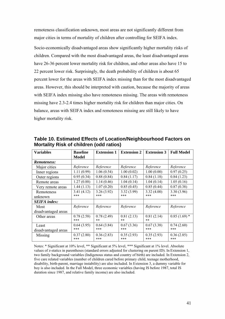
remoteness classification unknown, most areas are not significantly different from

major cities in terms of mortality of children after controlling for SEIFA index.

Socio-economically disadvantaged areas show significantly higher mortality risks of

children. Compared with the most disadvantaged areas, the least disadvantaged areas

have 26-36 percent lower mortality risk for children, and other areas also have 15 to

22 percent lower risk. Surprisingly, the death probability of children is about 65

percent lower for the areas with SEIFA index missing than for the most disadvantaged

areas. However, this should be interpreted with caution, because the majority of areas

with SEIFA index missing also have remoteness missing. The areas with remoteness

missing have 2.3-2.4 times higher mortality risk for children than major cities. On

balance, areas with SEIFA index and remoteness missing are still likely to have

higher mortality risk.

Table 10. Estimated Effects of Location/Neighbourhood Factors on Mortality Risk of children (odd ratios) Variables Baseline

Model Extension 1 Extension 2 Extension 3 Full Model

Remoteness: Major cities Reference Reference Reference Reference Reference Inner regions 1.11 (0.99) 1.06 (0.54) 1.00 (0.02) 1.00 (0.00) 0.97 (0.25) Outer regions 0.95 (0.34) 0.88 (0.84) 0.84 (1.17) 0.84 (1.18) 0.84 (1.23) Remote areas 1.27 (0.88) 1.14 (0.46) 1.04 (0.14) 1.04 (0.14) 1.05 (0.16) Very remote areas 1.44 (1.13) 1.07 (0.20) 0.85 (0.45) 0.85 (0.44) 0.87 (0.38) Remoteness unknown

3.41 (4.12) ***

3.26 (3.92) ***

3.32 (3.99) ***

3.32 (4.00) ***

3.30 (3.96) ***

SEIFA index: Most disadvantaged areas

Reference Reference Reference Reference Reference

Other areas 0.78 (2.58) ***

0.78 (2.49) **

0.81 (2.13) **

0.81 (2.14) **

0.85 (1.69) *

Least disadvantaged areas

0.64 (3.95) ***

0.64 (3.84) ***

0.67 (3.36) ***

0.67 (3.38) ***

0.74 (2.60) ***

Missing 0.37 (2.80) ***

0.36 (2.83) ***

0.35 (2.93) ***

0.35 (2.93) ***

0.36 (2.85) ***

Notes: * Significant at 10% level, ** Significant at 5% level, *** Significant at 1% level. Absolute values of z-statics in parentheses (standard errors adjusted for clustering on parent ID). In Extension 1, two family background variables (Indigenous status and country of birth) are included. In Extension 2, five care related variables (number of children cared before primary child, teenage motherhood, disability, birth-parent, marriage instability) are also included. In Extension 3, a dummy variable for boy is also included. In the Full Model, three economic variables (having IS before 1987, total IS duration since 1987, and relative family income) are also included.

41

5.1.5 Child characteristics

Sex and birth month are the only two explanatory variables available for all primary

children in the sample. Since birth month is always insignificant in preliminary

regressions, it is excluded from the final models reported in this paper.

Gender differences are compared in two ways. First, the model is estimated using the

whole sample with a dummy variable of boy included (see the last column in Table

11). Boys appear to have significantly higher mortality risk (about 40% higher) than

girls, and the coefficient of boy hardly changes with the inclusion of extra explanatory

variables. Second, the models are estimated with sub-samples of boys and girls,

respectively. The results are reported in the first two columns of Table 11.

Generally, for both boys and girls, the following characteristics of primary parents are

associated with significantly higher mortality risk: being born in Australia, being

teenage mothers, having had children before, having a disability, not being birth-

parents, having IS records since 1987, and living in socio-economically disadvantaged

areas. Other variables are generally insignificant.

However, two patterns are different between boys and girls. First, teenage

motherhood seems to have largeger impacts on boys than on girls. Second, unlike for

a boy, although having had children before is also associated with higher mortality of

a girl, the risk tends to decrease with the number of children her primary parent had

before herself. The difference in mortality is insignificant between a girl who had four

or more siblings before herself and another girl who is the first child of her primary

parent; the difference is still very significant for boys with similar characteristics.

42

Table 11. Estimated Mortality Risk of Children by Sex (odd ratios) Variables Boys Girls Whole

sample Boy - - 1.39 (3.91) *** Family background: Indigenous 0.71 (1.37) 1.22 (0.64) 0.88 (0.64) Born in Australia Reference Reference Reference Born in main English-speaking countries 0.28 (2.51) ** 0.28 (2.18) ** 0.28 (3.28) *** Born in other countries 0.66 (2.53) ** 0.64 (2.27) ** 0.65 (3.38) *** Care factors: Teenage motherhood 3.24 (5.08) *** 2.25 (2.78) *** 2.77 (5.64) *** Having no child before primary child Reference Reference Reference Having 1 child before primary child 3.67 (7.73) *** 3.58 (6.74) *** 3.62 (10.22)

*** Having 2 children before primary child 5.12 (8.61) *** 3.32 (5.13) *** 4.30 (9.94) *** Having 3 children before primary child 5.01 (6.97) *** 2.11 (2.12) ** 3.65 (6.82) *** Having 4+ children before primary child 2.89 (3.11) *** 1.20 (0.33) 2.10 (2.61) *** Disability 1.38 (1.40) 0.98 (0.06) 1.22 (1.06) Birth-parent 0.16 (11.74)

*** 0.15 (10.10) ***

0.16 (15.42) ***

Marriage stable Reference Reference Reference Marriage unstable 0.78 (1.68) * 0.96 (0.24) 0.85 (1.42) Marriage very unstable 0.99 (0.05) 1.03 (0.15) 1.01 (0.10) Economic factors: Having IS before 1987 1.41 (1.41) 0.77 (0.64) 1.15 (0.65) Total IS duration since 1987: no records Reference Reference Reference Total IS duration since 1987: less than 1 year 2.01 (3.40) *** 1.30 (1.01) 1.69 (3.28) *** Total IS duration since 1987: 1-2 years 1.39 (1.41) 2.46 (4.01) *** 1.83 (3.78) *** Total IS duration since 1987: 3-5 years 1.62 (2.16) ** 1.31 (1.03) 1.47 (2.29) ** Total IS duration since 1987: 6-8 years 1.89 (2.86) *** 1.32 (1.02) 1.64 (2.85) *** Total IS duration since 1987: 9-11 years 2.45 (4.07) *** 1.93 (2.46) ** 2.22 (4.72) *** Total IS duration since 1987: 12 or more years 1.98 (2.73) *** 1.54 (1.43) 1.78 (3.01) *** Low family income Reference Reference Reference Middle family income 1.23 (1.28) 1.12 (0.57) 1.19 (1.37) High family income 1.08 (0.31) 0.86 (0.54) 0.98 (0.11) Family income missing 1.06 (0.28) 1.19 (0.63) 1.12 (0.65) Location/neighbourhood factors: Major cities Reference Reference Reference Inner regions 0.98 (0.16) 0.97 (0.18) 0.97 (0.25) Outer regions 0.85 (0.89) 0.81 (0.87) 0.84 (1.23) Remote areas 1.04 (0.11) 1.07 (0.17) 1.05 (0.16) Very remote areas 1.30 (0.67) 0.38 (1.20) 0.87 (0.38) Remoteness unknown 3.21 (3.44) *** 3.40 (2.25) ** 3.30 (3.96) *** Most socio-economically disadvantaged areas Reference Reference Reference Other areas 0.85 (1.26) 0.83 (1.15) 0.85 (1.69) * Least socio-economically disadvantaged areas 0.66 (2.67) *** 0.84 (0.92) 0.74 (2.60) *** SEIFA index missing 0.37 (2.48) ** 0.36 (1.59) 0.36 (2.85) *** Observations 61015 57946 118961 Pseudo R2 0.0769 0.0669 0.0703

Notes: * Significant at 10% level, ** Significant at 5% level, *** Significant at 1% level. Absolute values of z-statics in parentheses (standard errors adjusted for clustering on parent ID).

43

5.1.6 Robust Tests

Extra robust tests have been undertaken.

First, continuous variables for economic factors (IS duration and family income) and

SEIFA index are used instead of category variables; the coefficients of other variables

are hardly affected.

Second, children who died after 10 years old are excluded from the sample. Some

deaths of children may not be recorded in TDS2 if the primary parents left payments

and never came back again. This kind of under-recording may be non-random; for

instance, people with higher income may have higher probability. This is also likely

to happen when children are older. Nonetheless, the test leads to qualitatively the

same findings.

However, there are two unsolved issues for the logistic model; that is, right censored

data and delaying in entry (different time of first claiming benefit). Duration model

provides a better solution for these issues, and is discussed in Section 5.2.

44

5.2 Hazard of Death of Primary Children

As administrative data, TDS2 has two outstanding issues that need to be considered

for this research: (1) delayed entry – people were only observed in TDS2 when they

started to claim benefits from the Government; and (2) right censoring – deaths of

children after parents left benefits were not observed. The logistic model in Section

5.1 cannot provide satisfactory solutions to these issues, while they can be easily

tackled with the duration model.

The analyses in this section are mainly based on non-parametric (Kaplan-Meier

estimator) and semi-parametric (Cox Proportional Hazard estimator) methods to allow

for most flexible forms of survival and hazard functions.

A similar estimation strategy is applied as in Section 5.1, that is, starting with a group

of factors (Baseline Model), and then including more explanatory variables in stages

(Extensions) to check the sensitivity of the coefficients of the factors in the Baseline

Model.

For consistency and simplicity, the variables are treated as constant over time in the

results reported below, while results of models with time-varying variables and other

specifications are discussed in robust tests.

In addition, to be consistent with the analyses in other sections, the sample is still

restricted to the primary children who were not born abroad and did not die within

two months after birth. One point to note here is that due to this restriction, the earliest

entry occurs after two months (from birth); this slightly changes the interpretation of

the estimation results (conditional on surviving to two months).

5.2.1 Family Background

Figure 6 shows the estimated Kaplan-Meier survival functions of children with

Indigenous and non-Indigenous parents. Apparently Indigenous children (children

with Indigenous parents) have significantly lower survival probability than non-

Indigenous children.

45

Figure 6. Kaplan-Meier Survival Estimates by Indigenous Status

0.99

00.

993

0.99

61.

000

1 3 5 7 9 11 13 15 17Age of child (years)

Non-Indigenous Indigenous

Table 12 lists the estimated hazard ratios for children from different family

backgrounds as indicated by parental Indigenous status and country of birth. In the

Baseline Model, only indigenous status and country of birth are included; Indigenous

status is very significant, and the hazard of premature death of an Indigenous child is

about 1.91 times as high as for a non-Indigenous child.

However, when other factors are taken into consideration, Indigenous status does not

matter very much. Again, this confirms the finding in Section 5.1; that is, the high

mortality of Indigenous children can be mostly explained by other disadvantages of

their parents such as low socio-economic status rather than Indigenous status per se.

The Kaplan-Meier estimators of survival functions for children of Australia born

people and others are shown in Figure 7. Estimation results in Table 12 are generally

consistent with the pattern shown in Figure 7: a child whose primary parent was born

abroad tend to have a lower hazard of death; in particular, the hazard of death is 64

percent lower for a child whose primary parent was born in a main English-speaking

country than for a child with an Australia born parent. Interestingly, contrary to

Indigenous status, country of birth becomes more significant when more explanatory

variables are included in the model.

46

Figure 7. Kaplan-Meier Survival Estimates by Country of Birth 0.

990

0.99

30.

996

1.00

0

1 3 5 7 9 11 13 15 17Age of child (years)

Born abroad Born in Australia

Table 12. Estimated Effects of Family Background on Death Hazards of Children (hazard ratios) Variables Baseline

Model Extension 1 Extension 2 Extension 3 Full Model

Indigenous 1.91 (3.71) ***

1.00 (0.02) 1.00 (0.02) 0.92 (0.47) 0.89 (0.61)

Country of birth: Born in Australia Reference Reference Reference Reference Reference Born in main English-speaking countries

0.55 (1.59) 0.37 (2.59) **

0.37 (2.59) **

0.36 (2.66) ***

0.36 (2.68) ***

Born in other countries

1.02 (0.20) 0.82 (1.65) * 0.82 (1.68) * 0.77 (2.16) **

0.75 (2.30) **

Notes: * Significant at 10% level, ** Significant at 5% level, *** Significant at 1% level. Absolute values of z-statics in parentheses (standard errors adjusted for clustering on parent ID). In Extension 1, five care related variables (number of children cared before primary child, teenage motherhood, disability, birth-parent, marriage instability) are also included. In Extension 2, a dummy variable for boy is also included. In Extension 3, three economic variables (having IS before 1987, total IS duration since 1987, and relative family income) are also included. In the Full Model, three location/neighbourhood variables (SEIFA index, remoteness, and rural/urban areas) are also included.

47

5.2.2 Care Related Factors Several factors, including teenage motherhood, disability, marriage instability, being a

birth-parent, and number of children ever cared for before a primary child, are likely

to affect the care quality. As shown in Table 13, except for disability, all other factors

have significant effects on the mortality risk of children.

Table 13. Estimated Effects of Care Related Factors on Death Hazards of Children (hazard ratios) Variables Baseline

Model Extension 1 Extension 2 Extension 3 Full Model

Teenage motherhood

2.61 (5.55) ***

2.53 (5.30) ***

2.55 (5.34) ***

2.36 (4.83) ***

2.33 (4.76) ***

Disability 1.41 (1.89) * 1.40 (1.83) * 1.40 (1.84) 1.21 (1.02) 1.20 (0.98) Birth-parent 0.06 (18.69)

*** 0.06 (18.73) ***

0.06 (18.70) ***

0.06 (18.49) ***

0.06 (18.48) ***

# of children before primary child:

None Reference Reference Reference Reference Reference One 3.29 (10.18)

*** 3.22 (9.93) ***

3.24 (9.96) ***

3.17 (9.77) ***

3.16 (9.75) ***

Two 4.12 (10.17) ***

4.03 (9.93) ***

4.04 (9.93) ***

3.90 (9.69) ***

3.89 (9.65) ***

Three 3.76 (7.24) ***

3.65 (7.00) ***

3.67 (7.02) ***

3.45 (6.65) ***

3.42 (6.60) ***

Four or more 2.75 (3.73) ***

2.70 (3.59) ***

2.72 (3.62) ***

2.48 (3.25) ***

2.45 (3.18) ***

Marriage instability:

Stable Reference Reference Reference Reference Reference Unstable 1.13 (1.14) 1.13 (1.21) 1.13 (1.18) 0.90 (0.95) 0.90 (0.92) Very unstable 1.39 (3.07)

*** 1.39 (3.08) ***

1.39 (3.03) ***

1.08 (0.59) 1.08 (0.61)

Notes: * Significant at 10% level, ** Significant at 5% level, *** Significant at 1% level. Absolute values of z-statics in parentheses (standard errors adjusted for clustering on parent ID). In Extension 1, two family background variables (Indigenous status and country of birth) are included. In Extension 2, a dummy variable for boy is also included. In Extension 3, three economic variables (having IS before 1987, total IS duration since 1987, and relative family income) are also included. In the Full Model, three location/neighbourhood variables (SEIFA index, remoteness, and rural/urban areas) are also included.

Having one, two, three, and four or more children before a primary child is likely to

increase the death hazard of the primary child by approximately 2.12, 2.89, 2.42, and

1.45 times respectively (in the Full Model). Therefore, it seems that for an extra

sibling, increase in competition for resources (including share of family income and

48

time of parents) predominates over accumulation of the caring experience of parents.

However, when the number of children is three or more, the hazards become lower;

this may be because in largeger families, older siblings need less care and can also

help parents take care of the younger children.

A striking point of the results is that the variable of birth-parent (claiming benefits for

a primary child from birth) is very significant in all models and birth-parent is

associated with approximately 94 percent lower mortality of children. Using a

different definition of birth-parent – claiming benefits for a primary child within three

(or 4, 5 or 6) months after birth – leads to qualitatively similar findings, though the

difference between birth-parent and non birth-parent is smaller.

Being cared for by a teenage mother is associated with 1.33-1.55 times higher hazard

of premature death. Figure 8 shows the difference in estimated Kaplan-Meier survival

functions between children of teenage mothers and others.

In addition, marriage instability and parental disability also tend to increase the

mortality risk of children, while the effects are not very significant.

Figure 8. Kaplan-Meier Survival Estimates by Teenage Motherhood

0.99

00.

993

0.99

61.

000

1 3 5 7 9 11 13 15 17Age of child (years)

Not teenage mothers Teenage mothers

49

5.2.3 Economic Factors

The income support receipt is a good indicator of low income because to be eligible

for income support, a person has to pass strict income test and asset test (for details,

refer to Centrelink website at www.centrelink.gov.au). Therefore, total IS duration

between 1987 and 2005 reflects how long a primary parent had been on low income

in the period, indicating their long-term economic disadvantage.

The estimated Kaplan-Meier survival functions are compared in Figure 9 for children

whose primary parents had and had no IS spells since 1987. As expected, having been

on IS since 1987 is associated with a significantly higher mortality risk of children.

Figure 9. Kaplan-Meier Survival Estimates by IS Incidence

0.99

00.

993

0.9

961.

000

1 3 5 7 9 11 13 15 17Age of child (years)

Never on IS since 1/10/87 Once on IS since 1/10/87

In Table 14, total IS duration since 1987 is further broken down into seven categories,

and the one for people with no IS records is used as the reference group. The six

categories for people with IS records since 1987 contain roughly the same number of

primary children (about 11,000).

50

Table 14. Estimated Effects of Economic Factors on Death Hazards of Children (hazard ratios) Variables Baseline

Model Extension 1 Extension 2 Extension 3 Full Model

Having IS before 1987

1.49 (1.90) * 1.46 (1.82) * 1.18 (0.77) 1.18 (0.80) 1.15 (0.66)

Total IS duration since 1987:

No record Reference Reference Reference Reference Reference Less than 1 year 1.69 (3.32)

*** 1.69 (3.32) ***

1.64 (3.06) ***

1.64 (3.07) ***

1.63 (3.03) ***

1-2 years 1.88 (4.20) ***

1.89 (4.21) ***

1.84 (3.82) ***

1.84 (3.81) ***

1.80 (3.68) ***

3-5 years 1.51 (2.61) ***

1.50 (2.57) ***

1.40 (1.99) **

1.40 (1.99) **

1.37 (1.84) *

6-8 years 1.65 (3.14) ***

1.63 (3.06) ***

1.47 (2.21) **

1.48 (2.25) **

1.43 (2.06) **

9-11 years 2.12 (5.08) ***

2.08 (4.88) ***

1.93 (3.83) ***

1.93 (3.83) ***

1.85 (3.55) ***

12 or more years 1.58 (2.53) **

1.53 (2.34) **

1.50 (2.06) **

1.50 (2.07) **

1.44 (1.83) *

Relative family income:

Low Reference Reference Reference Reference Reference Middle 0.89 (0.92) 0.90 (0.86) 1.04 (0.32) 1.04 (0.34) 1.06 (0.44) High 0.81 (1.14) 0.81 (1.12) 0.88 (0.72) 0.88 (0.70) 0.90 (0.56) Missing 1.50 (2.38)

** 1.52 (2.49) **

1.24 (1.24) 1.24 (1.27) 1.24 (1.25)

Notes: * Significant at 10% level, ** Significant at 5% level, *** Significant at 1% level. Absolute values of z-statics in parentheses (standard errors adjusted for clustering on parent ID). In Extension 1, two family background variables (Indigenous status and country of birth) are included. In Extension 2, five care related variables (number of children cared before primary child, teenage motherhood, disability, birth-parent, marriage instability) are also included. In Extension 3, a dummy variable for boy is also included. In the Full Model, three location/neighbourhood variables (SEIFA index, remoteness, and rural/urban areas) are also included.

Although people with IS records generally have 43-85 percent higher mortality risk of

children than those with no IS records (in the Full Model), the death hazard of

children does not monotonically increase with total IS duration. People who had been

on IS for 9-11 years or 1-2 years have the highest mortality risk of children; in

contrast, people who had 3-5 years consistently have the lowest hazard; the hazard

ratio for these two groups is approximately 1.35 (1.85/1.37). Interestingly, people who

had stayed on IS for 12 years or longer since 1987 also had relatively lower mortality

of children.

Having income support records before 1987 indicates two characteristics of parents:

(1) having low income before the births of primary children; and (2) being older. The

51

former is associated with higher mortality risk of children, while the latter is the

opposite. On balance, having IS before 1987 slightly increases the mortality of

children but the effect is insignificant.

In addition, as shown in Figure A1 in the Appendix, contrary to the result based on

total IS duration since 1987, having income support between 1987 and the last caring

date is associated with higher survival probability of children, indicating that parental

income support incidence was more likely to be affected by the death of a child than

the other way around. Table A3 in The Appendix provides a comparison of estimated

death hazards of children with different measures of IS history, where a similar

conclusion can be drawn.

Overall, the results of this paper demonstrate the complexity of the correlation

between parental IS experience and mortality of children, and also suggests the

necessity of further exploration of this issue.

As shown in Figure 10, lower family income is associated with a higher mortality risk

of children; the group with family income missing has the highest mortality.

However, after controlling for total IS duration since 1987, the income variable

generally becomes insignificant (see Table 14).

Figure 10. Kaplan-Meier Survival Estimates by Family Income

0.99

00.

993

0.99

61.

000

1 3 5 7 9 11 13 15 17Age of child (years)

Low income Middle incomeHigh income Missing

52

5.2.4 Location/Neighbourhood Factors

As shown in Figure 11, people living in a socio-economically disadvantaged area tend

to suffer higher mortality risk of children. Estimation results of Cox PH models

generally show the same results (see Table 15): compared with people living in the

most disadvantaged areas, those living in the least disadvantaged areas have 36-25

percent lower mortality risks of children, and those in other areas also have 23-17

percent lower risks.

However, unlike the pattern in Figure 11, areas with SEIFA index missing have the

lowest hazards in Table 15. This should be interpreted together with the results for the

missing categories of remoteness, because the missing categories in both variables

basically refer to the same group of areas (based on the same group of postcodes). On

balance, the mortality risk in the areas with SEIFA index missing is not significantly

different from the most disadvantaged areas.

Figure 12 compares the estimated Kaplan-Meier survival functions of different

remoteness categories. Remote areas (including very remote areas) and areas with

remoteness classification missing stand out, showing the lowest survival probabilities;

differences between other areas are not large. Results in Table 15 generally show that

after controlling for SEIFA index (and other variables), except for the missing

category, other remoteness categories are not significantly different from each other in

death hazards of children. Therefore, high mortality risk of children in remote/very

remote areas can be mostly attributed to the socio-economic disadvantage in those

areas.

The differences between rural and urban areas are also insignificant, although death

hazards are slightly higher in rural areas. State/territory of residence is excluded from

the model reported here because it is always insignificant in preliminary regressions.

53

Figure 11. Kaplan-Meier Survival Estimates by SEIFA Index

0.99

00.

993

0.99

61.

000

1 3 5 7 9 11 13 15 17Age of child (years)

Most disadv antaged Mid-lev el disadvantageLeast disadvantaged Missing

Figure 12. Kaplan-Meier Survival Estimates by Remoteness

0.99

00.

993

0.99

61.

000

1 3 5 7 9 11 13 15 17Age of child (years)

Major cities Inner regionsOuter regions Remote areasMissing

54

Table 15. Estimated effects of Location/Neighbourhood Factors on Death Hazards of Children (hazard ratios) Variables Baseline

Model Extension 1

Extension 2

Extension 3

Full Model

Rural areas 1.16 (1.06) 1.16 (1.04) 1.19 (1.24) 1.19 (1.21) 1.18 (1.14) Remoteness: Major cities Reference Reference Reference Reference Reference Inner regions 1.03 (0.30) 1.02 (0.18) 0.96 (0.38) 0.96 (0.35) 0.95 (0.50) Outer regions 0.88 (0.83) 0.85 (1.08) 0.82 (1.32) 0.82 (1.33) 0.82 (1.33) Remote areas 1.21 (0.69) 1.12 (0.39) 1.06 (0.20) 1.06 (0.21) 1.07 (0.23) Very remote areas 1.38 (0.98) 1.03 (0.09) 0.79 (0.65) 0.79 (0.65) 0.82 (0.56) Unknown 3.12 (3.82)

*** 3.06 (2.52) ***

3.05 (3.79) ***

3.03 (3.79) **

3.05 (3.80) ***

SEIFA Index of Disadvantage:

Most disadvantaged areas

Reference Reference Reference Reference Reference

Other areas 0.77 (2.72) ***

0.78 (2.52) **

0.80 (2.24) **

0.80 (2.27) **

0.83 (1.87) *

Least disadvantaged areas

0.64 (3.88) ***

0.66 (3.63) ***

0.69 (3.13) ***

0.69 (3.16) ***

0.75 (2.48) **

SEIFA index missing 0.48 (1.88) * 0.45 (1.97) **

0.46 (1.98) **

0.46 (1.21) 0.45 (2.00) **

Notes: * Significant at 10% level, ** Significant at 5% level, *** Significant at 1% level. Absolute values of z-statics in parentheses (standard errors adjusted for clustering on parent ID). In Extension 1, two family background variables (Indigenous status and country of birth) are included. In Extension 2, five care related variables (number of children cared before primary child, teenage motherhood, disability, birth-parent, marriage instability) are also included. In Extension 3, a dummy variable for boy is also included. In the Full Model, three economic variables (having IS before 1987, total IS duration since 1987, and relative family income) are also included.

5.2.5 Child Characteristics

There are two variables regarding child characteristics available for all primary

children that can be used in the regressions – sex and birth month. However, birth

month is always insignificant in preliminary regression, so it is excluded in the final

model.

To see the differences between boys and girls, three sets of estimations have been

undertaken: (1) with the whole sample but including a dummy variable for boys, (2)

with boys only, and (3) with girls only. In the first set of estimations, boys on average

have 41 percent higher death hazards than girls, and this figure does vary much when

extra explanatory variables are included.

55

Table 16. Estimated Hazard Ratios by Sex of Children Variables Boys Girls Whole

sample Boy - - 1.41 (4.00) *** Family background: Indigenous 0.72 (1.29) 1.21 (0.62) 0.89 (0.61) Born in Australia Reference Reference Reference Born in main English-speaking countries 0.36 (2.04) ** 0.35 (1.77) * 0.36 (2.68) *** Born in other countries 0.76 (1.74) * 0.74 (1.56) 0.75 (2.30) ** Care factors: Teenage motherhood 2.83 (4.51) *** 1.79 (2.06) ** 2.33 (4.76) *** Having no child before primary child Reference Reference Reference Having 1 child before primary child 3.28 (7.47) *** 3.01 (6.29) *** 3.16 (9.75) *** Having 2 children before primary child 4.74 (8.44) *** 2.93 (4.84) *** 3.89 (9.65) *** Having 3 children before primary child 4.71 (6.83) *** 1.93 (1.91) * 3.42 (6.60) *** Having 4+ children before primary child 3.32 (3.57) *** 1.39 (0.61) 2.45 (3.18) *** Disability 1.35 (1.32) 0.97 (0.08) 1.20 (0.98) Birth-parent 0.06 (13.75)

*** 0.05 (12.49) ***

0.06 (18.48) ***

Marriage stable Reference Reference Reference Marriage unstable 0.82 (1.27) 1.01 (0.08) 0.90 (0.92) Marriage very unstable 1.06 (0.40) 1.08 (0.38) 1.08 (0.61) Economic factors: Having IS before 1987 1.44 (1.50) 0.76 (0.66) 1.16 (0.72) Total IS duration since 1987: no records Reference Reference Reference Total IS duration since 1987: less than 1 year 1.90 (3.10) *** 1.27 (0.92) 1.62 (2.98) *** Total IS duration since 1987: 1-2 years 1.36 (1.36) 2.41 (3.91) *** 1.80 (3.68) *** Total IS duration since 1987: 3-5 years 1.48 (1.75) * 1.24 (0.84) 1.37 (1.85) * Total IS duration since 1987: 6-8 years 1.73 (2.44) ** 1.10 (0.34) 1.44 (2.09) ** Total IS duration since 1987: 9-11 years 2.03 (3.15) *** 1.62 (1.78) * 1.85 (3.57) *** Total IS duration since 1987: 12 or more years 1.63 (1.89) * 1.22 (0.65) 1.44 (1.85) * Middle family income 1.11 (0.65) 0.97 (0.13) 1.05 (0.42) High family income 0.99 (0.04) 0.79 (0.83) 0.90 (0.58) Family income missing 1.18 (0.74) 1.31 (1.01) 1.24 (1.26) Low family income Reference Reference Reference Location/neighbourhood factors: Major cities Reference Reference Reference Inner regions 0.98 (0.14) 0.89 (0.63) 0.95 (0.50) Outer regions 0.84 (0.89) 0.77 (1.04) 0.82 (0.56) Remote areas 1.09 (0.22) 1.04 (0.10) 1.07 (0.23) Very remote areas 1.25 (0.56) 0.33 (1.31) 0.82 (1.33) Remoteness unknown 2.94 (3.39) *** 3.17 (2.11) ** 3.05 (3.80) *** Most socio-economically disadvantaged areas Reference Reference Reference Other areas 0.84 (1.41) 0.82 (1.26) 0.83 (1.87) * Least socio-economically disadvantaged areas 0.67 (2.60) *** 0.85 (0.85) 0.75 (2.48) ** SEIFA index missing 0.42 (1.92) * 0.52 (0.92) 0.45 (2.00) ** Rural areas 1.09 (0.48) 1.34 (1.25) 1.18 (1.14) # of Observations 61005 57937 118942

Notes: * Significant at 10% level, ** Significant at 5% level, *** Significant at 1% level. Absolute values of z-statics in parentheses (standard errors adjusted for clustering on parent ID).

56

The results of the three sets of estimations (from the Full Models) are compared in

Table 16. Overall, the estimated effects of key variables are qualitatively similar for

boys and girls, but there are also some differences that exist.

Commonly, a higher mortality risk was found for both boys and girls whose parents

had the following characteristics: being born in Australia, being teenage mothers,

having had child(ren) before, not being the birth-parent, having IS records since 1987,

and living in socio-economically disadvantaged areas.

The differences between boys and girls include: (1) parental country of birth is

significant for boys but generally insignificant for girls; (2) teenage motherhood

shows bigger impacts on boys than on girls; (3) for girls, parents having had three or

more children before are not significantly different from parents having had no child

before, but for boys the differences are still very significant; and (4) unlike for boys,

mortality risks of girls are not significantly different between different parental IS

durations, except that the category of IS duration between one and two years is

associated with significantly (1.41 times) higher hazards of death than the reference

group – having no IS records since 1987.

5.2.6 Robust Tests

Similar robust tests have been undertaken as those shown in Section 5.1; for instance,

some category variables, such as total IS duration, family income and SEIFA index,

are replaced with continuous variables and their quadratic forms; the coefficients of

other variables change little.

Additional tests are undertaken particularly for duration models.

Firstly, so far the variables in the duration models are treated as constant. This is not a

big issue when the sampling window is relative short; however, observations in TDS2

spanned more than 15 years (from 1991 or earlier to 2005) and some variables such as

marital status, number of children and home address are very likely to change during

the period. One robust test that has been undertaken is using the last instead of first

records of some time varying variables such as remoteness and SEIFA index, and

another and a better choice is directly incorporating time varying variables in the

duration model.

57

Secondly, apart from information of primary parents, TDS2 also contains information

of other parents who once claimed family payments for the primary children in the

sampling period. This information is used in some models for robust tests.

Thirdly, piecewise constant method is also applied for estimation. In general, the main

findings are consistent in all these tests.

Overall, the estimation results of duration models generally confirm the findings in

Section 5.1 (using logistic model). A summary of findings and detailed discussion are

provided in the next section.

58

6. Summary and Discussion

Several key findings of this research are summarised and discussed in this section.

(1) The rate of premature death of Indigenous children (0.89%) is nearly twice as

high as that of non-Indigenous children (0.47%).

This finding provides further evidence the confirm the higher mortality of Indigenous

children in Australia. An issue of interest is why this is the case and what Indigenous

status implies.

Previous studies show that compared with non-Indigenous children, Indigenous

children are more likely to have low birthweight (13% compared to 6% in 2000-02)

(Laws and Sullivan 2005), be less physically active and have poorer nutrition (leading

to obesity and diabetes), live in overcrowded housing, and have unsafe drinking water

and inadequate waste disposal (AIHW 2006). Indigenous people mostly live in remote

and very remote areas, where smoking and drinking alcohol in hazardous quantities

are much more common than in other areas in Australia (AIHW 2005). All these

factors lead to significantly higher health risks for Indigenous children and can at least

partly explain their higher mortality rates.

An interesting discovery of this research is that after taking into consideration other

factors, the difference in mortality risk between Indigenous and non-Indigenous

children becomes insignificant. The results suggest that higher mortality of

Indigenous children may be explained mainly by their disadvantages in other aspects

such as low socio-economic status rather than Indigenous status per se.

(2) Children of immigrants generally have a lower mortality rate (0.39%) than

other children (0.51%)

Even after controlling for other factors, this conclusion still holds, and is consistent

with findings in other studies, such as AIHW (2006).

AIHW (2006) attributes this finding mainly to two ‘selection’ effects: one refers to

self-selection – migrants are usually those who are willing, and are physically and

economically able, to migrate; and the other is government selection with certain

eligibility criteria (for example, on health and education), which are generally

59

associated with better health of people and their children. Some research (Fennelly

2005, cited in AIHW 2006) found that the difference between immigrants and others

may diminish with length of stay.

Two extra conjectures are proposed here: (1) survival of the fittest – immigrants tend

to choose the most favourable place to migrate, and if they find the place is not

suitable for them, they are likely to move away; (2) lack of social capital means that

immigrants value more their family members, especially children, merely because

they are their most important social network in a new country. In addition, sometimes

a better living condition for children is the main reason for migration.

(3) Lower income and longer income support duration are associated with

significantly higher mortality of children

The mortality rate of children from low income families (income equal or less than

50% of sample mean) is twice as high (0.64%) as that of children from high income

families (income more than 150% of sample mean) (0.32%). The mortality of children

belonging to parents with nine years or longer on income support since 1987 is 0.75

percent, in comparison with 0.32 percent for people not receiving income support

during the same period. Since low family income is one of the key eligibility criteria

for receiving income support, it is not surprising that after controlling for income

support duration, the income variable becomes insignificant.

Low family income inevitably tightens budget constraint and has the potential to

reduce family expenditure on nutritious food, medical care and housing, increases

financial stress, affects the quality and stability of care for children. These

circumstances ultimately have negative impacts on the health of children.

However, there are two possible effects of income support receipt on the mortality

risk of children. First, the increase in family income enables parents to stay at home

with their children, which tends to reduce the mortality rate of children. Second,

income support incidence is also an indicator of unemployment/underemployment,

low income and probably low earning ability, which is likely to be associated with a

higher mortality of children.

As family income is controlled for in the model, the variable of total income support

duration since 1987 mainly serves as an indicator of long-term economic

disadvantage.

60

The non-linearity of the correlation between total income support duration and

mortality of children shows the complexity of the correlation. One point to note is that

parental income support incidence is more likely to be a consequence of the death of a

child rather than a cause, because estimation of some duration models shows that

currently receiving and having ever received income support are both associated with

lower death hazard of a child. This issue deserves further exploration.

(4) Birth-parents have significantly lower mortality of children than others

(0.33% vs. 0.97%)

Birth-parent in this paper refers to a person who started taking care of a primary child

from the time of birth. This definition, as discussed earlier, may put some actual birth-

parents into the category of non birth-parents. Using a slightly different definition of

birth-parent, such as people who started taking care of a primary child within three or

five months after birth, does not qualitatively change the result. The result is not

sensitive to controlling for other variables in the model either.

Since mortality of children is significantly higher at a younger age, especially within

the first one month, birth-parents should be subject to a higher risk of child mortality.

However, this research shows an opposite result, suggesting the existence of more

important counter factors, such as higher care quality of birth-parents, which tend to

reduce the risk of child mortality. There is evidence in the literature that children

living with step-mothers are significantly less likely to have routine doctor visits, or to

have a place for usual medical care or for sick care (Case and Paxson 2001).

(5) Teenage mothers are significantly more likely to have higher mortality of

children than others (0.74% vs. 0.48%)

Estimation results from both logistic and duration models show starting to take care of

a primary child as a teenage mother is associated with 1.3 to 2.3 times higher

mortality risk of children. The estimations are not very sensitive with the inclusion of

extra variables in the model. This may be explained by the relatively poorer

knowledge, skill and experience of teenage mothers in taking care of a child.

(6) Taking care of more children before a primary child is associated with

significantly higher mortality risk of the child

In the sample used for this research, the mortality of children for parents who had

never taken care of any other children is 0.36 percent, in comparison with 0.59

61

percent for those who had one child before and 0.68 percent for those who had two or

more children before.

The number of children ever cared for before a primary child has two opposite effects

on the mortality risk of the primary child. First, having had other children before

increases the knowledge, skill and experience of care, and thus tends to reduce the

mortality risk of the primary child. Second, having more siblings also means more

competition for caring resources including food and parental time; a smaller share of

caring resources implies higher mortality risk.

The estimation results show that the second effect – competition for caring resources

– dominates. In the meantime, boys are more likely to be affected by the number of

siblings than girls, probably because boys need more caring resources to survive.

(7) Parental disability and marriage instability are also associated with higher

mortality risk of children

Disability in this paper is defined as being eligible for Disability Support Pension

(DSP). People with a disability may have more time to take care of their children but

their disability may also limit their ability to care (and may be associated with poorer

health of children if the disability is due to genetic reasons). On balance, disability has

a negative effect on the health of children. The mortality of children for people with a

disability (0.90%) is nearly twice as high as that for others (0.47%) in the sample.

Marriage stability also affects the quality and stability of caring for children. Patton et

al (2005) show that the rates of having a diagnosable and mental or behavioural

disorder, for children living in sole parent and blended families (ie, families formed

by second marriages between parents with children), were twice as high as in other

families.

In the sample of TDS2, people whose marriage was very unstable (having five or

more marital events in TDS2) have a mortality of children of 0.72 percent, in

comparison to 0.42 percent for those whose marriage was stable (having one or two

marital events in TDS2). Overall, however, the effects of parental disability and

marriage instability are not very significant after controlling for other factors.

(8) Mortality of children is significantly different between most and least

disadvantaged neighbourhood

62

This paper uses the SEIFA Disadvantage Index, remoteness and rural/urban area to

capture several aspects of neighbourhood characteristics.

The SEIFA index is a comprehensive measure of relative socio-economic

disadvantage of a neighbourhood, with a focus on low income earners, relatively

lower educational attainment and high unemployment.

In the TDS2 sample, the mortality of children in the most disadvantaged areas (up to

30th percentiles of SEIFA Disadvantage Index) is 0.61 percent, in comparison to 0.38

percent in the least disadvantaged areas (the top 30 percentiles of SEIFA index). The

estimation results of both logistic and duration models confirm this pattern.

The finding is also consistent with those in other Australian studies, such as AIHW

(2006), which reports that both infant death rates and childhood death rates are

significantly higher in the most disadvantaged areas than in the least disadvantaged

areas. A study by Patton et al (2005) shows that poorer families are more likely to

report that their neighbourhoods feel unsafe at least some of the time.

In the sample of TDS2, the mortality of children in remote/very remote areas is 0.91

percent, nearly twice as high as that in major cities (0.46%). Rural areas also have

higher mortality of children (0.58%) than urban areas (0.47%). People living in rural

and remote areas are subject to higher health risks (such as smoking and drinking in

hazardous quantities, being physically inactive, and driving in higher speeds), and

also have less access to health services (AIHW 2005; Garnaut et al 2001, cited in

AIHW 2006). In addition, as discussed in earlier, these differences may reflect the

generally higher mortality of Indigenous children.

The current research finds that after controlling for SEIFA index, the differences in

mortality of children between remoteness categories and between rural and urban

areas become insignificant, indicating that the higher mortality of children in rural and

remote areas may be largely explained by the socio-economic disadvantage of people

living in the areas.

To sum up, the results of this research generally suggest that the risk of premature

death (before the 18th birthday) is significantly higher for children from disadvantaged

families as indicated by several characteristics of the primary carer. These include

lower income (especially those persistently in low income), Indigenous status, teenage

63

motherhood, living in socio-economically disadvantaged areas, and having three or

more children to care for. The influencing factors are inter-related and the socio-

economic factors are particularly important.

Death is the worst health outcome of children, and there are some other less severe

health outcomes such as chronic illness and disability. They were unobserved in this

study, but lower the current life quality of children and will also affect the

productivity of children when they grow up. The significant correlation between

higher death rates and parental disadvantage implies potential correlations between

poorer general health conditions of children and parental disadvantage. In

combination, these indicate evidence of intergenerational transmission of

disadvantage in Australia. To break the cycle of intergenerational transmission of

disadvantage, reducing the mortality and improving the health of children from

disadvantaged families must be given high priority.

Due to the limitations of the data and the complex inter-relationships between

mortality of children and the underlying influencing factors, the correlations revealed

in this paper can not be interpreted as causal relationships. However, this should not

hinder the application of the findings in policy arena; a higher quantity and quality of

chickens and eggs can be produced without knowing which one is the origin.

Nevertheless, policy responses to this complex issue can hardly be very simple;

multiple policies may be required to tackle health problems and economic

disadvantages respectively and simultaneously, but both of them should be well-

targeted.

64

References

ABS (Australian Bureau of Statistics), 1994. Australian Social Trend, 1994. ABS Cat. No. 4102.0. ABS, Canberra.

ABS, 2003. Births, Australia, 2002. ABS Cat. No. 3301.0. ABS, Canberra.

ABS, 2003a. Deaths, Australia, 2002. ABS Cat. No. 3302.0. ABS, Canberra.

ABS, 2004. Migration, 2002-03. ABS Cat. No. 3412.0. ABS, Canberra.

ABS, 2004a. Deaths, Australia, 2003. ABS Cat. No. 3302.0. ABS, Canberra.

ABS, 2004b. Births, Australia, 2003. ABS Cat. No. 3301.0. ABS, Canberra.

ABS, 2006. Deaths, Australia, 2005. ABS Cat. No. 3302.0. ABS, Canberra.

ABS, 2007. Health of Children in Australia: A Snapshot, 2004-05. ABS Cat. No. 4829.0.55.001. ABS, Canberra.

AIHW (Australian Institute of Health and Welfare), 2005. Rural, Regional and Remote Health – Indicators of Health. AIHW Cat. No. PHE 59. AIHW, Canberra.

AIHW, 2006. Australia’s Health 2006. AIHW Cat. No. AUS 73. AIHW, Canberra.

Beaulieu, N., Duclos, J.-Y., Fortin, B., Rouleau, M. 2001. An Econometric Analysis of Intergenerational Reliance on Social Assistance. Département ďéconomique, Université Laval, Cahier de recherché no. x.

van den Berg, G.J., Lindeboom, M., Portrait, F., 2006. Economic Conditions Early in Life and Individual Mortality. American Economic Review, 96(1), 290-302.

Blakemore, T., 2005. Examining Potential Risk Factors, Pathways and Processes Associated with Childhood Injury in the Longitudinal Study of Australian Children. Paper presented to the Australian Social Policy Conference, Sydney, July.

Case, A., Paxson, C. 2001. Mothers and Others: Who Invests in Children’s Health? Journal of Health Economics, 20(2001), 301-328.

Case, A., Lubotsky, D., Paxson, C., 2002. Economic Status and Health in Childhood: The Origins of the Gradient. The American Economic Review, 92(5) 1308-1334.

Case, A., Fertig, A., Paxson, C., 2005. The Lasting Impact of Childhood Health and Circumstance. Journal of Health Economics, 24(2005), 365-389.

Cobb-Clark, D., Gorgens, T., 2004. The Path to Self-Reliance for Young People: A Review of the Literature. Report prepared for the Department of Family and Community Services.

Corak, M., Gustafsson, B., Österberg, T., 2000. Intergenerational Influences on the Receipt of Unemployment Insurance in Canada and Sweden. IZA Discussion Paper No. 184.

Currie, J., Stabile, M., 2003. Socioeconomic Status and Child Health: Why is the Relationship Stronger for Older Children? American Economic Review, 93(5), 1813-1823.

65

Deaton, A., 2002. Commentary: The convoluted Story of International Studies of Inequality and Health. International Journal of Epidemiology, 31, 546-549.

Draper, G., Turrell, G., Oldenburg, B., 2004. Health Inequalities in Australia: Mortality. Health Inequalities Monitoring Series No. 1. AIHW Cat. No. PHE 55. Queensland University of Technology and the Australian Institute of Health and Welfare: Canberra.

Eades, S., 2004. Maternal and Child Health Care Services: Actions in the Primary Health Care Setting to Improve the Health of Aboriginal and Torres Strait Islander Women of Childbearing Age, Infants and Young Children. Aboriginal and Torres Strait Islander Primary Health Care Review: Consultant Report no. 6, Commonwealth of Australia, Canberra.

Fennelly, K., 2005. The ‘Healthy Migrant’ Effect. Healthy Generations, 5, 1-4.

Garnaut, J., Connell, P., Lindsay, R., Rodriguez, V., 2001. Country Australia: Influences on Employment and Population Growth. ABARE Research Report 2001. Australian Bureau of Agriculture and Research Economics, Canberra.

Gottschalk, P., 1992. The Intergenerational Transmission of Welfare Participation: Facts and Possible Causes. Journal of Policy Analysis and Management, 11(2), 254-272.

Gottschalk, P., 1996. Is the Correlation on Welfare Participation across Generations Spurious? Journal of Public Economics, 63(1), 1-25.

Laws P.J., Sullivan, E.A., 2005. Australia’s Mothers and Babies 2003. Perinatal Statistics Series no. 29. AIHW Cat. No. PER 29. AIHW, Canberra.

Lochner, K., Pamuk, E., Makuc, D., Kennedy, B.P., Kawachi, I., 2001. State-Level Income Inequality and Individual Mortality Risk: A Prospective, Multilevel Study. American Journal of Public Health, 91(3), 385-391.

McCoull, F., Pech, J., 2000. Transgenerational Income Support Dependence in Australia: Early Evidence. In: Saunders, P. (Ed.), Reforming the Australian Welfare State, 91-111. Australian Institute of Family Studies, Melbourne.

Maloney, T., Pacheco, G., 2003. Are the Determinants of Intergenerational Welfare Dependency Gender-Specific? Australian Journal of Labour Economics, 6(2), 371-382.

Patton, G.C., et al, 2005. A Picture of Australia’s Children. Medical Journal of Australia, 182(9), 437-438.

Pech, J., McCoull, F., 1998. Transgenerational Poverty and Income Support Dependence in Australia: Work in Progress. Social Security Journal, 1998(2).

Pech, J., McCoull, F., 2000. Transgenerational Welfare Dependence: Myths and Realities. Australian Social Policy, 2000/1, 43-67.

Penman, R., 2005. Psychosocial Factors and ‘Intergenerational Transmission of Welfare Dependency’: A Review of Literature. Report to Department of Family and Community Services.

Rank, M.R., Cheng, L., 1995. Welfare Use across Generations: How Important Are the Ties that Bind? Journal of Marriage and the Family, 57, 673-683.

Rodgers, G.B., 1979. Income and Inequality as Determinants of Mortality: An International Cross-section Analysis. Population Studies, 33(3), 343-351.

66

Turrell, G., Mathers, C., 2001. Socioeconomic Inequalities in All-cause and Specific-cause Mortality in Australia: 1985-1987 and 1995-1997. International Journal of Epidemiology, 30, 231-239.

Turrell, G., Stanley, L., de Looper, M., Oldenburg, B., 2006. Health Inequalities in Australia: Morbidity, Health Behaviours, Risk factors and Health Services Use. Health Inequalities Monitoring Series no. 2. AIHW Cat. No. PHE 72. Queensland University of Technology and AIHW, Canberra.

Waldmann, R.J., 1992. Income Distribution and Infant Mortality. Quarterly Journal of Economics, 107(4), 1283-1302.

Wildman, J., 2003. Modelling Health, Income and Income Inequality: the Impact of Income Inequality on Health and Health Inequality. Journal of Health Economics, 22(2003), 521-538.

Zubrick, S.R., et al, 2004. The Western Australian Aboriginal Child Health Survey: The Health of Aboriginal Children and Young People. Telethon Institute for Child Health Research, Perth.

67

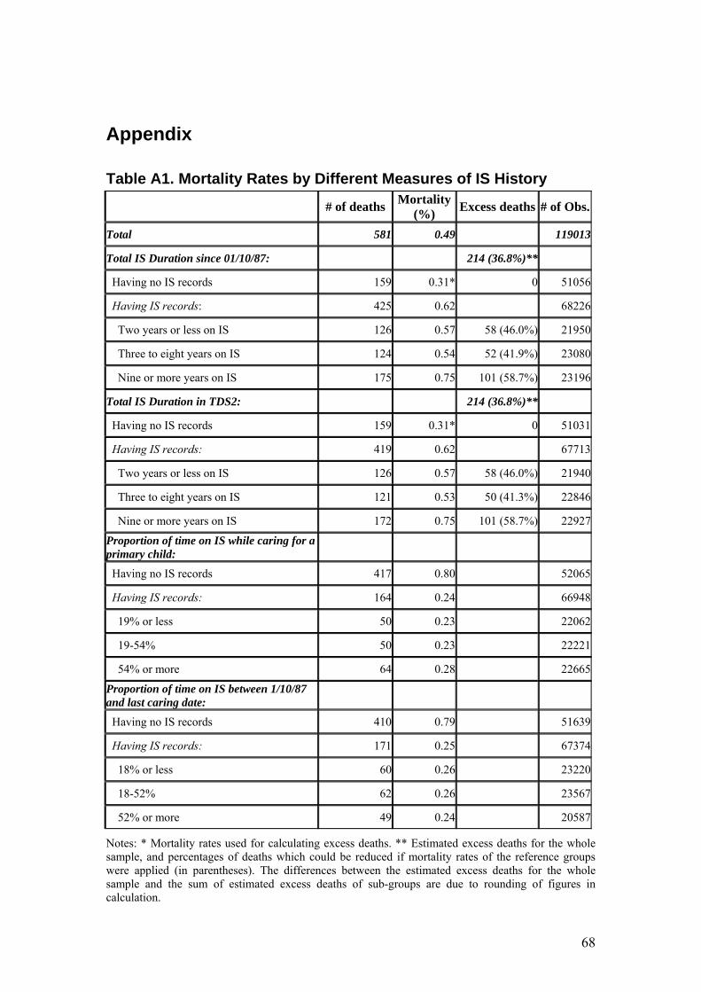
Appendix

Table A1. Mortality Rates by Different Measures of IS History

# of deaths Mortality (%) Excess deaths # of Obs.

Total 581 0.49 119013

Total IS Duration since 01/10/87: 214 (36.8%)**

Having no IS records 159 0.31* 0 51056

Having IS records: 425 0.62 68226

Two years or less on IS 126 0.57 58 (46.0%) 21950

Three to eight years on IS 124 0.54 52 (41.9%) 23080

Nine or more years on IS 175 0.75 101 (58.7%) 23196

Total IS Duration in TDS2: 214 (36.8%)**

Having no IS records 159 0.31* 0 51031

Having IS records: 419 0.62 67713

Two years or less on IS 126 0.57 58 (46.0%) 21940

Three to eight years on IS 121 0.53 50 (41.3%) 22846

Nine or more years on IS 172 0.75 101 (58.7%) 22927

Proportion of time on IS while caring for a primary child:

Having no IS records 417 0.80 52065

Having IS records: 164 0.24 66948

19% or less 50 0.23 22062

19-54% 50 0.23 22221

54% or more 64 0.28 22665

Proportion of time on IS between 1/10/87 and last caring date:

Having no IS records 410 0.79 51639

Having IS records: 171 0.25 67374

18% or less 60 0.26 23220

18-52% 62 0.26 23567

52% or more 49 0.24 20587

Notes: * Mortality rates used for calculating excess deaths. ** Estimated excess deaths for the whole sample, and percentages of deaths which could be reduced if mortality rates of the reference groups were applied (in parentheses). The differences between the estimated excess deaths for the whole sample and the sum of estimated excess deaths of sub-groups are due to rounding of figures in calculation.

68

Table A2. Estimated Mortality Risks by Different Measures of IS History (logistic model, odd ratios) (1) (2) (3) (4) Having IS before 1987 1.15 (0.65)

Total IS Duration since 01/10/87:

Having no IS records Reference

Having IS records:

Less than one year on IS 1.69 (3.28) ***

1-2 years or less on IS 1.83 (3.78) ***

3-8 years on IS 1.47 (2.29) **

9-11 years on IS 1.64 (2.85) ***

12 years or longer on IS 1.78 (3.01) ***

Total IS Duration in TDS2:

Having no IS records Reference

Having IS records:

Less than one year on IS 1.69 (3.28) ***

1-2 years or less on IS 1.84 (3.80) ***

3-8 years on IS 1.46 (2.21) **

9-11 years on IS 1.65 (2.90) ***

12 years or longer on IS 2.28 (4.88) ***

IS incidence while caring for a primary child:

Having IS records 0.14 (10.93) ***

Proportion of time on IS (%) 0.98 (4.28) ***

IS incidence between 1/10/87 and last caring date:

Having IS records 0.22 (9.25) ***

Proportion of time on IS (%) 0.97 (6.83) ***

Notes: * Significant at 10% level, ** Significant at 5% level, *** Significant at 1% level. Absolute values of z-statics in parentheses (standard errors adjusted for clustering on parent ID). Other variables controlled for include Indigenous status, country of birth, relative family income, number of children cared before primary child, teenage motherhood, disability, birth-parent, marriage instability, a dummy variable of boy, SEIFA index, and remoteness.

69

Table A3. Estimated Death Hazards by Different Measures of IS History (Cox PH model, hazard ratios) (1) (2) (3) (4) Having IS before 1987 1.20 (0.88)

Total IS Duration since 01/10/87:

Having no IS records Reference

Having IS records:

Less than one year on IS 2.03 (4.30) ***

1-2 years or less on IS 2.19 (4.77) ***

3-8 years on IS 1.59 (2.68) ***

9-11 years on IS 1.59 (2.63) ***

12 years or longer on IS 1.97 (3.91) ***

Total IS Duration in TDS2:

Having no IS records Reference

Having IS records:

Less than one year on IS 2.03 (4.32) ***

1-2 years or less on IS 2.20 (4.81) ***

3-8 years on IS 1.58 (2.65) ***

9-11 years on IS 1.61 (2.71) ***

12 years or longer on IS 2.04 (4.10) ***

IS incidence while caring for a primary child:

Having IS records 0.13 (10.35) ***

Proportion of time on IS (%) 0.98 (5.01) ***

IS incidence before last caring date:

Having IS records 0.24 (8.14) ***

Proportion of time on IS (%) 0.97 (8.36) ***

Notes: * Significant at 10% level, ** Significant at 5% level, *** Significant at 1% level. Absolute values of z-statics in parentheses (standard errors adjusted for clustering on parent ID). Other variables controlled for include Indigenous status, country of birth, relative family income, number of children cared before primary child, teenage motherhood, disability, birth-parent, marriage instability, a dummy variable of boy, SEIFA index, and remoteness.

70

Figure A1. Kaplan-Meier Survival Estimates by IS Receipt of Primary Parents between 1 October 1987 and the Last Caring Dates

0.99

00.

993

0.9

961.

000

1 3 5 7 9 11 13 15 17Age of child (years)

Never on IS 1/10/87 - last caring date Once on IS

71