morrey spaces and generalized cheeger sets

MORREY SPACES AND GENERALIZED CHEEGER SETS

QINFENG LI AND MONICA TORRES

Abstract. We maximize the functional É h(x)dx

P (E),

where E ⊂ Ω is a set of finite perimeter, Ω is an open bounded set with Lipschitz boundary and his nonnegative. Solutions to this problem are called generalized Cheeger sets in Ω. We show thatthe Morrey spaces L1,λ(Ω), λ ≥ n − 1, are natural spaces for h to study this problem. We provethat if h ∈ L1,λ(Ω), λ > n− 1, then generalized Cheeger sets exist. We also study the embeddingof Morrey spaces into Lp spaces. We show that, for any 0 < λ < n, the Morrey space L1,λ(Ω) isnot contained in any Lq(Ω), 1 < q < p = n

n−λ . We also show that if h ∈ L1,λ(Ω), λ > n− 1, thenthe reduced boundary in Ω of a generalized Cheeger set is C1,α and the singular set has Hausdorffdimension at most n − 8 (empty if n ≤ 7). For the critical case h ∈ L1,n−1(Ω), we demonstratethat this strong regularity fails. We also prove a structure result for generalized Cheeger sets inRn; namely, a bounded generalized Cheeger set E ⊂ Rn with h ∈ L1(Rn) is always pseudoconvex,and any pseudoconvex set is a generalized Cheeger set for some h ∈ L1(Rn), h nonnegative andnot equivalent to zero. A similar structure theorem holds for generalized Cheeger sets in Ω.

1. Introduction

In this paper we study the existence and regularity of solutions of the problem

(1.1) v∗h1 := supE⊂Ω

V h1 (E), V h1 (E) =

Éh (x) dx

Hn−1(∂∗E),

where Ω is an open bounded set with Lipschitz boundary and h is an integrable function that belongsto the Morrey spaces. We consider in particular the case h ≥ 0. If h ≡ 1, (1.1) reduces to

supE⊂Ω

Ln(E)

Hn−1(∂∗E):= M1(Ω),

whose solutions are called Cheeger sets. Cheeger established the inequality λ1(Ω) ≥(

12M1(Ω)

)2

,where λ1(Ω) is the first eigenvalue of the Laplacian under Dirichlet boundary conditions. Refer-ences to Cheeger sets include Caselles-Chambolle-Novaga [18, 19], Alter-Caselles [2], Figalli-Maggi-Pratelli [25], Parini [42], Alter-Caselles-Chambolle [3], Carlier-Comte-Peyre [16], Carlier-Comte [17],Butazzo-Carlier-Comte [14], Kawohl-Friedman [33], Kawohl-Novaga [35] and Kawohl-Lachand [34].

A set E where the supremum (1.1) is attained (i.e. v∗h1 = V h1 (E)) is called a generalizedCheeger set in Ω. Indeed, generalized Cheeger sets refer to more general problems of the typesupE⊂Ω

Éh1 dx´

∂∗E h2 dHn−1 . Generalized Cheeger have been studied when h1 ∈ L∞ and h2 continuous(see Buttazo-Carlier-Comte [14] and the references therein). We will show in this paper that it isnatural to study (1.1) with h belonging to the Morrey spaces (see also Ionescu-Lachand-Robert [32]).

Since a necessary condition for generalized Cheeger sets to exist is that

(1.2) supE⊂Ω

V h1 (E) <∞,

Date: June 2015.Key words and phrases. function spaces, geometric measure theory, calculus of variation, minimal surfaces.

1

2 QINFENG LI AND MONICA TORRES

we start our study by analyzing the space S(Ω), consisting of all functions g that satisfy, for eachset E ⊂ Rn of finite perimeter,

(1.3) sup

É∩Ω|g|

Hn−1(∂∗E)<∞.

Indeed, h satisfies (1.2) if and only if h ∈ S(Ω) (see Lemma 3.6). We note our notation

Mp(Ω) := L1,λ(Ω), λ > 0, λ = n

(1− 1

p

),

where L1,λ(Ω) is the Morrey space introduced in section 2. In this paper we show that S(Ω) coincideswith the Morrey space Mn(Ω) (see Theorem 3.7).

In order to study characterizations of Morrey spaces in terms of S(Ω), we first note that theisoperimetric inequality implies that

É∩Ω

|g|Hn−1(∂∗E) is bounded above by

É∩Ω

|g|dx

|E|1−1n

. This observation

suggests that S(Ω) can be compared to the Morrey space L1,n−1(Ω), whose definition uses cubes Q,and |Q|1− 1

n instead of |E|1− 1n . This observation can be made rigorous using the boxing inequality

(see Theorem 3.1), which provides a covering theorem of sets of finite perimeter with balls (or cubes),and that allows to control the perimeters of the elements of the cover in a universal way and in termsof the perimeter of the covered set.

We show in this paper the existence of generalized Cheeger sets whenever h belongs to the Morreyspaces Mp(Ω), p > n (see Theorem 4.4). We also study the critical case p = n (see section 5 andExample 4.5)

Another space that naturally arises in connection to problem (1.1) is Mp(Ω) (see definition 2.11),which is the same as the weak Lp space, denoted as Lp,w(Ω) (see Remark 2.12). The existence ofgeneralized Cheeger sets for h ∈ Ln(Ω) was proven in Bright-Li-Torres [12]. In particular, note thatthe spaces Lp,w(Ω), p > n, are contained in Ln(Ω). The new existence result in this paper generalizes[12] since the spaces Mp(Ω), p > n, are not contained in Ln(Ω). This follows from Section 4, wherewe show that Mp(Ω), p > n, can not be embbeded into any space Lq(Ω), with 1 < q < p. This alsoshows that Mp(Ω) (Mp(Ω).

In the second part of this paper we investigate the regularity of generalized Cheeger sets in Ω.For convenience, we consider the equivalent problem

(1.4) Ch0 := inf Jh(F ), Jh(F ) =P (F )´Fhdx

, F ⊂ Ω is a set of finite perimeter,

with h ∈ Mn(Ω), h ≥ 0 and h not equivalent to the zero function. We study the regularity of ageneralized Cheeger set E in Ω by noticing that E is also a minimizer of the functional

(1.5) IH(F ) = P (F ) +

ˆF

H(x)dx, F ⊂ Ω,

with H(x) = −Ch0 h(x). The minimization (1.5), with Ω replaced by Rn, is called the variationalmean curvature problem, and H is called the variational mean curvature of E. The regularity ofthis problem, for H ∈ Lp(Ω), has been studied by several authors including De Giorgi [22], Massari[38, 39], Barozzi-Gonzalez-Tamanini [9], Gonzalez-Massari-Tamanini [28] and Gonzalez-Massari [27].The regularity of more general classes of quasi minimizers of perimeter was studied in Tamanini [44],Bombieri [15], Paolini [41] and Ambrosio-Paolini [6]. Using the regularity theory for quasi minimizersdeveloped in Tamanini [44], we show that, if E is a generalized Cheeger set for some h ∈ Mp(Ω),p > n, then ∂∗E∩Ω is a C1,α-hypersurface and the singular set has dimension at most n−8 (empty ifn ≤ 7). This strong regularity corresponds to the classical results for the variational mean curvatureproblem mentioned above for H ∈ Lp(Ω), p > n.

We also study the structure of generalized Cheeger sets in Rn (i.e. Ω replaced by Rn in theminimization (1.4)). For the variational mean curvature problem, it is well known that, for any

MORREY SPACES AND GENERALIZED CHEEGER SETS 3

set of finite perimeter E, there exists an L1(Rn) function H such that E has mean curvature H(see [9] and [27]). This implies that we can not expect to have regularity for sets with L1 meancurvature, since a set of finite perimeter can have a wild boundary (see, for example, [37, Example12.25]). Motivated by the close relationship between our generalized Cheeger set problem and thevariational mean curvature problem, we ask if this is also true in our situation, namely, if for any setof finite perimeter E with 0 < |E| <∞, there exists an L1 nonnegative function h such that E is ageneralized Cheeger set in Rn corresponding to this h. We answer negatively this question by showinga structure theorem (see Theorem 7.7) which gives a necessary and sufficient condition for E to be ageneralized Cheeger set. More specifically, we show that if E is a generalized Cheeger set in Rn forsome h ∈ L1(Rn), then E is a pseudoconvex set (see Definition 7.2), and if E is a pseudoconvex set,then a non negative function in L1(Rn) can be constructed so that E minimizes Jh in Rn. Theorem7.7 has some interesting consequences, in particular the fact that each indecomposable component(see Definition 2.9) of a generalized Cheeger set for some h ∈ L1(Rn) is a generalized Cheeger set forthe same h, and hence each indecomposable component of a pseudoconvex set is also pseudoconvex(see Theorem 8.1). A similar structure theorem holds for generalized Cheeger sets in Ω (see Theorem7.9).

For the variational mean curvature problem, De Giorgi conjectured in 1992 that if H ∈ Ln, thenthe boundary of a minimizer E of IH is locally parametrizable (out of a singular set, if n ≥ 8) bya bi-lipschitz map defined on an open ball of Rn−1. De Giorgi also proposed an example of a quasiminimizer in the plane having a singular point at the origin and parametrizable by a bi-lipschitzmap. Gonzalez-Massari-Tamanini [28] proved that the example of De Giorgi, whose boundary isthe union of two bilogarithmic spirals, is indeed a set with mean curvature in L2(R2). The fullconjecture is still an open problem, but the case n = 2 has been solved by Ambrosio-Paolini [6,Theorem 5.2]. For n > 2, Paolini showed in [41] that the boundary of E is locally parametrizablefor any α < 1 with a map τ such that both τ and τ−1 are Cα. This result was extended to quasiminimizers of perimeter by Ambrosio-Paolini [6, Theorem 4.10].

Motivated by the De Giorgi conjecture, we would like to know if the regularity obtained in [41, 6]also holds for generalized Cheeger sets corresponding to our critical case h ∈ Mn(Ω). Althoughthis assumption on h is weaker than h ∈ Ln(Ω), our structure theorem for generalized Cheeger sets(see Theorem 7.7) suggests that one could expect some type of partial regularity in this criticalcase. In this paper we prove that the strong regularity fails by showing that there exists a functionh ⊂ Mn(Ω), and a generalized Cheeger set in Ω whose ∂E contains a large set (of Hausdorffdimension n) consisting of points of zero density.

As an application of our results, we consider in the last section the following averaged shapeoptimization problem (see [12]):

(1.6) v∗ := infE⊂Ω

V (E), V (E) = V2(E) + V g1 (E) = infE⊂Ω

´∂∗E

f(x,νE(x))dHn−1(x) +´Egdx

Hn−1(∂∗E),

This problem was studied in [12] under the condition g ∈ Ln(Ω). It was proven there that, if thereexists a minimizing sequence Ei such that |Ei| → 0 or Hn−1(Ei) → ∞, then there exists anotherminimizing sequence consisting of convex polytopes with n + 1 faces shrinking to a point. In thispaper we extend this result to the case g ∈ Mp(Ω), p > n, and we show (see Corollary 9.4) that, ifthere exists a minimizing sequence Ei satisfying Hn−1(∂∗Ei)→∞ or P (Ei)→ 0, then there existsanother minimizing sequence of convex polytopes with n + 1 faces shrinking to a point. We notethat this result does not require g to be negative, although we are interested in the case g ≤ 0, tobe consistent with our existence results of generalized Cheeger sets (see Remark 4.7).

We organize the paper as follows. In section 2 we introduce preliminaries needed for the paper.In section 3 we study a characterization of Morrey spaces. In section 4 we proof the existence ofgeneralized Cheeger sets. In section 5 we study the embedding of Morrey spaces into Lp spaces. Insection 6 we study the regularity of generalized Cheeger sets in Ω. In section 7 we prove a structure


theorem for generalized Cheeger sets and in section 8 we study the critical case h ∈Mn(Ω). Finally,in section 9, we present an application to averaged shape optimization.

2. Preliminaries

In this paper we work with sets of finite perimeter. We refer the reader to the standard referencesby Maggi [37], Ambrosio-Fusco-Pallara [5] and Evans [23] for the relevant definitions and propertiesof sets of finite perimeter used in this paper. Also, Hn−1 denotes the (n− 1)-dimensional Hausdorffmeasure in Rn, and Ln is the Lebesgue measure in Rn. We will use the notation Ln(E) = |E|. Fora set of finite perimeter E, we use indistinctly the notation P (E) = Hn−1(∂∗E). The convex hullof a set E is denoted as E.

Remark 2.1. Throughout this paper, Ω denotes a bounded open set with Lipschitz boundary.

Remark 2.2. In particular, we note that we can write E ⊂ Ω or E ⊂ Ω since ∂Ω is Lipschitz andhence E is Ln-equivalent to E ∪ ∂Ω.

Definition 2.3. A set of finite perimeter E is said to be decomposable if there exists a partition ofE into two measurable sets A,B with strictly positive measure such that

(2.1) P (E) = P (A) + P (B)

If no such a partition exists, we call E a indecomposable set.

Remark 2.4. The notion of indecomposable set extends the topological notion of connectedness. Itcan be easily shown that a connected open set of finite perimeter is indecomposable.

Definition 2.5. For H ∈ L1(Rn), let IH be the functional defined as

(2.2) IH(F ) = P (F ) +

ˆF

H(x)dx, F ⊂ Rn is a set of finite perimeter.

A set E of finite perimeter is said to have variational mean curvature H if E is a minimizer of (2.2).

Remark 2.6. It can be easily seen (by computing the first variation of the functional IH) that if Ehas variational mean curvature H, H is continuous at x ∈ ∂E and ∂E is smooth near x, then thevalue of the (classical) mean curvature of ∂E at x is given by −H(x)

n−1 .

The fact that every set of finite perimeter has a variational mean curvature was observed for thefirst time in Barozzi-Gonzalez-Tamanini [9]. Moreover, we have the following

Theorem 2.7. Let E be a set of finite perimeter with |E| < ∞, then there exists a functionHE ∈ L1(Rn), such that HE is the variational mean curvature for E. Furthermore,

(2.3) HE < 0 a.e. on E,HE > 0 a.e. on Rn \ E,and

(2.4) ‖H‖L1(E) = P (E), ‖HE‖L1(Rn) = 2P (E).

Proof. See [27, Theorem 2.3] for the proof of (2.4). The property (2.3) is proven in [27, (2.16) and(2.17)].

The following theorem by Ambrosio-Caselles-Masnou-Morel [4, Proposition 3.5, Theorem 1 (sec-tion 4)], is an important tool we will use in this article.

Theorem 2.8. Let E be a set of finite perimeter in Rn. Then there exists a unique countablefamily of pairwise disjoint indecomposable sets Ei such that |Ei| > 0, E = ∪iEi, P (E) =

∑i P (Ei),

∂∗E = ∪i∂∗Ei (modHn−1) and Hn−1(∂∗Ei ∩ ∂∗Ej) = 0. Moreover, if F ⊂ E is an indecomposableset then F is contained (mod Hn) in some set Ei.

Remark 2.9. We call each Ei in the previous theorem a indecomposable component of E.


We now proceed to review the definition of Morrey spaces, which will be shown to be the naturalspaces to study the existence and regularity of generalized Cheeger sets in Ω. The spaces Lz,λ(Ω)were introduced by Morrey in [40] and are defined as

(2.5) Lz,λ(Ω) =

u : sup

r>0,x0∈Ω

1

rλ

ˆBr(x0)∩Ω

|u(y)|zdy <∞

When λ = 0, the Morrey space is the same as the usual Lz space. When λ = n, the spatial dimension,the Morrey space is equivalent to L∞, due to the Lebesgue differentiation theorem. When λ > n,the space contains only the 0 function.

In this paper we study the Morrey space L1,λ(Ω), where 0 < λ < n. Recall that L1,λ = L1,λ

where the latter is the Companato space. (See Definition 4.1 and [43, Theorem 4.3]). If p > 1 issuch that λ = n(1− 1

p ) we have that u ∈ L1,λ(Ω) if and only if

supr>0,x0∈Ω

1

|Br(x0)|1−1p

ˆBr(x0)∩Ω

|u(y)|dy <∞,

or equivalently,

L1,λ(Ω) :=

u ∈ L1(Ω) : sup

´Q∩Ω|u|dx

|Q|1−1/p: Q is a cube

< +∞

.

Definition 2.10.

(2.6) Mp(Ω) := L1,λ(Ω), λ = n(1− 1

p), p > 1.

We now define the spaces of functions Mp(Ω), p > 1, which are the counterparts of the Morreyspaces Mp, p > 1, as follows:

Definition 2.11. For p > 1, let

(2.7) Mp(Ω) :=

g Lebesgue measurable : sup

A⊂Ω,A measurable

´A|g|dx

|A|1−1/p< +∞

.

We note thatMp(Ω) ⊂ L1(Ω) by choosing A = Ω in the definition above. Moreover, if g ∈Mp(Ω),we define

(2.8) ||g||Mp(Ω) := supA⊂Ω,A measurable

´A|g|dx

|A|1−1/p.

Remark 2.12. The standard weak Lp space, denoted as Lp,w(Ω), satisfies (see [12, Lemma 8.3]):

(2.9) Lp,w(Ω) = Mp(Ω), p > 1.

Remark 2.13. Remark 2.12 implies that Mp(Ω), p > 1, can be embedded in to any space Lq(Ω),with 1 ≤ q < p.

Remark 2.14. Notice that

(2.10) Mp(Ω) ⊂Mq(Ω), 1 < q < p,

and

(2.11) Mp(Ω) ⊂Mq(Ω), 1 < q < p.

We also study in this paper the relationship between Mp(Ω) and Mp(Ω). Clearly, we have

(2.12) Mp(Ω) ⊂Mp(Ω), p > 1,

and it is natural to ask whether Mp(Ω) = Mp(Ω), since they are defined in a similar manner. Ifthis is not true, we still ask the question whether Mp(Ω), for p large enough, can be embedded intoMq(Ω), for some q close enough to 1. We will see in section 5 that the answer to both questions isfalse, by showing that Mp(Ω), p > 1, cannot be embedded into any space Lq(Ω), for 1 < q < p.


3. A characterization of Morrey spaces

Since the necessary condition for generalized Cheeger sets to exist is that

(3.1) v∗h1 = supE⊂Ω

Éhdx

Hn−1(∂∗E)<∞, h nonnegative,

in this section we study appropriate spaces for h to guarantee (3.1).A key tool that we will use in this paper is the boxing inequality, which was originally due to

Gustin [31] (see also [45, Chapter 5, Lemma 5.9.3].

Theorem 3.1. Let n > 1 and 0 < τ < 12 . Suppose E is a set of finite perimeter such that

lim supr→0|E∩Br(x)||Br(x)| > τ whenever x ∈ E. Then there exists a constant C(τ, n) and a sequence of

closed balls Bri(xi) with xi ∈ E such that

(3.2) E ⊂∞⋃i=1

Bri(xi)

and

(3.3)∞∑i=1

rn−1i ≤ CHn−1(∂∗E).

Remark 3.2. If E is an open set, the proof of Theorem 3.1 actually shows that we can take τ = 12 .

Moreover, the covering Bri can be chosen in such a way that

(3.4)|E ∩Bri/5(x)||Bri/5(x)|

=1

2

We now introduce the following spaces which are related to the functional (3.1).

Definition 3.3.

(3.5) S(Ω) :=

g ∈ L1(Ω) : sup

É∩Ω|g|dx

P (E): E is a set of finite perimeter

< +∞

.

and

(3.6) Sc(Ω) :=

g ∈ L1(Ω) : sup

´K∩Ω

|g|dxP (K)

: K is a bounded convex set< +∞

.

Remark 3.4. We define the semi-norm of u with respect to S(Ω) by

‖g‖S(Ω) := sup

É∩Ω|g|dx

P (E): E is a set of finite perimeter

.

We similarly define ‖g‖Sc(Ω).

Remark 3.5. Since a bounded convex set has finite perimeter (see Excercise 15.14 in [37]), S(Ω) ⊂Sc(Ω).

From the definition of S(Ω), we have the following:

Lemma 3.6. h ∈ S(Ω) if and only if (3.1) holds.

Proof. Clearly, if h ∈ S(Ω) then (3.1) holds. We now assume that v∗h <∞. It suffices to show thatÉ∩Ω

hdx

P (E) is uniformly bounded for any connected polytope E with small perimeter. Indeed, we canrestrict to small perimeter because h ∈ L1, and we can restrict to connected polytopes because setsof finite perimeter can be approximated by open polytopes (see [37, Remark 13.13]), and each openpolytope E is a countable disjoint union of its connected components Ei. Morever, we have

(3.7)É∩Ω

hdx

P (E)≤ sup

i

Éi∩Ω

hdx

P (Ei).


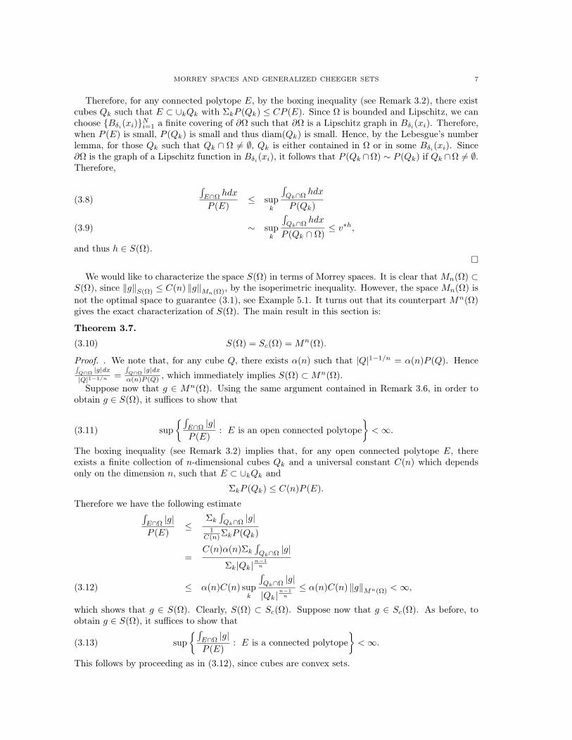
Therefore, for any connected polytope E, by the boxing inequality (see Remark 3.2), there existcubes Qk such that E ⊂ ∪kQk with ΣkP (Qk) ≤ CP (E). Since Ω is bounded and Lipschitz, we canchoose Bδi(xi)Ni=1 a finite covering of ∂Ω such that ∂Ω is a Lipschitz graph in Bδi(xi). Therefore,when P (E) is small, P (Qk) is small and thus diam(Qk) is small. Hence, by the Lebesgue’s numberlemma, for those Qk such that Qk ∩ Ω 6= ∅, Qk is either contained in Ω or in some Bδi(xi). Since∂Ω is the graph of a Lipschitz function in Bδi(xi), it follows that P (Qk ∩Ω) ∼ P (Qk) if Qk ∩Ω 6= ∅.Therefore,

É∩Ω

hdx

P (E)≤ sup

k

´Qk∩Ω

hdx

P (Qk)(3.8)

∼ supk

´Qk∩Ω

hdx

P (Qk ∩ Ω)≤ v∗h,(3.9)

and thus h ∈ S(Ω).

We would like to characterize the space S(Ω) in terms of Morrey spaces. It is clear that Mn(Ω) ⊂S(Ω), since ‖g‖S(Ω) ≤ C(n) ‖g‖Mn(Ω), by the isoperimetric inequality. However, the space Mn(Ω) isnot the optimal space to guarantee (3.1), see Example 5.1. It turns out that its counterpart Mn(Ω)gives the exact characterization of S(Ω). The main result in this section is:

Theorem 3.7.

(3.10) S(Ω) = Sc(Ω) = Mn(Ω).

Proof. . We note that, for any cube Q, there exists α(n) such that |Q|1−1/n = α(n)P (Q). Hence´Q∩Ω

|g|dx|Q|1−1/n =

´Q∩Ω

|g|dxα(n)P (Q) , which immediately implies S(Ω) ⊂Mn(Ω).

Suppose now that g ∈ Mn(Ω). Using the same argument contained in Remark 3.6, in order toobtain g ∈ S(Ω), it suffices to show that

(3.11) sup

É∩Ω|g|

P (E): E is an open connected polytope

<∞.

The boxing inequality (see Remark 3.2) implies that, for any open connected polytope E, thereexists a finite collection of n-dimensional cubes Qk and a universal constant C(n) which dependsonly on the dimension n, such that E ⊂ ∪kQk and

ΣkP (Qk) ≤ C(n)P (E).

Therefore we have the following estimateÉ∩Ω|g|

P (E)≤

Σk´Qk∩Ω

|g|1

C(n)ΣkP (Qk)

=C(n)α(n)Σk

´Qk∩Ω

|g|

Σk|Qk|n−1n

≤ α(n)C(n) supk

´Qk∩Ω

|g|

|Qk|n−1n

≤ α(n)C(n) ‖g‖Mn(Ω) <∞,(3.12)

which shows that g ∈ S(Ω). Clearly, S(Ω) ⊂ Sc(Ω). Suppose now that g ∈ Sc(Ω). As before, toobtain g ∈ S(Ω), it suffices to show that

(3.13) sup

É∩Ω|g|

P (E): E is a connected polytope

<∞.

This follows by proceeding as in (3.12), since cubes are convex sets.


4. Existence of generalized Cheeger sets

We first introduce the following spaces:

Definition 4.1. We define

(4.1) S(Ω) :=

g ∈ L1(Ω) : lim sup

P (E)→0

É∩Ω|g|dx

P (E)= 0, E is a set of finite perimeter

.

and

(4.2) Sc(Ω) :=


P (K)→0

´K∩Ω

|g|dxP (K)

= 0, K is a bounded convex set

.

Remark 4.2. The arguments used in (3.11) imply that

S(Ω) =


P (E)→0

É∩Ω|g|dx

P (E)= 0, E is an open connected polytope

.

We now proceed to show the relation between the Morrey spaces introduced in section 2 and thespaces S(Ω) and Sc(Ω).

Theorem 4.3.

(4.3) Mp(Ω) ⊂ S(Ω), p > n, and S(Ω) = Sc(Ω).

Proof. Let g ∈Mp(Ω), p > n. From Remark 4.2, it suffices to show that

(4.4)É∩Ω|g|dx

P (E)→ 0,

whenever P (E)→ 0 and E is an open connected polytope. For such E, we apply boxing inequality(see Remark 3.2) to obtain cubes Qk and a universal constant C(n) such

(4.5) ΣkP (Qk) ≤ C(n)P (E).

Therefore,

|Qk| = (α(n)P (Qk))nn−1

≤ (C(n)α(n)P (E))nn−1(4.6)

Thus, we have the following estimates:É∩Ω|g|

P (E)≤

Σk´Qk∩Ω

|g|1

C(n)ΣkP (Qk)

=C(n)α(n)Σk

´Qk∩Ω

|g|

Σk|Qk|n−1n

≤ C(n)α(n) supk

´Qk∩Ω

|g|

|Qk|n−1n

= α(n)C(n) supk

[´Qk∩Ω

|g|

|Qk|p−1p

|Qk|1n−

1p

]≤ α(n)C(n)||g||Mp(Ω) (C(n)α(n)P (E))

nn−1 ( 1

n−1p ), by (4.6).(4.7)

Since 1n −

1p > 0,

É∩Ω

|g|P (E) → 0 if P (E)→ 0, which implies that g ∈ S(Ω). Clearly S(Ω) ⊂ Sc(Ω). If

g ∈ Sc(Ω) then, for any open connected polytope E, we proceed as before using (4.5) to obtain


(4.8)É∩Ω|g|

P (E)≤

Σk´Qk∩Ω

|g|1

C(n)ΣkP (Qk)= C(n) sup

k

´Qk∩Ω

|g|P (Qk)

→ 0

whenever P (E)→ 0, since (4.5) yields P (Qk)→ 0, g ∈ Sc(Ω), and the cubes Qk are convex sets.

In particular, Theorem 4.3 implies the existence of generalized Cheeger sets:

Theorem 4.4. (Existence of generalized Cheeger sets) Let h ∈Mp(Ω), p > n, with h ≥ 0 and h notequivalent to the zero function. A bounded open set Ω with Lipschitz boundary contains a generalizedCheeger set maximizing

(4.9) v∗h1 = supE⊂Ω

Éh(x)dx

P (E)

Proof. We first note that v∗h1 > 0. Let Ei be a minimizing sequence of (4.9), thus P (Ei) are uniformlybounded for otherwise we would have v∗h1 = 0. We also have that lim infi→∞ P (Ei) := P∞>0, forotherwise we would have that, up to a subsequence, P (Ei) → 0 and Theorem 4.3 would implyv∗h1 = 0. Therefore, by the standard compactness theorem for sets of finite perimeter there existsa set E0 such that, up to a subsequence, Ei → E0 in L1(Ω) and P (Ei) → P∞. If P (E0) = 0 then|E0| = 0 and hence the dominated convergence theorem yields´

Eih(x)dx

P (Ei)→É0h(x)dx

P∞= 0,

that is, v∗h1 = 0, which is not possible since v∗h1 > 0. We conclude that P (E0) > 0 and hence

(4.10) v∗h1 = limi→∞

Éih(x)dx

P (Ei)=P (E0)

P∞

É0h(x)dx

P (E0).

The lower semicontinuity of the perimeter gives P (E0) ≤ P∞, and henceÉ0h(x)dx

P (E0)=

P∞P (E0)

v∗h1 ≥ v∗h1 .

Therefore, P (E0) = P∞ and v∗h1 is attained by E0 in the maximization (4.9).

The following example shows that in the critical case h ∈Mn(Ω), there is no definite conclusionas to whether generalized Cheeger set exists.

Example 4.5. Let Ω = B1(0). Let h1(x) = n−1|x| and h2(x) = n−1

|x| − 1. Hence, h1, h2 ≥ 0, and itis easy to check that h1, h2 ∈Mn(Ω) \ ∪q>nMq(Ω). The arguments in [12, Example 7.6] justify thefollowing computation

(4.11)Éh1(x)dx

P (E)=

É

div x|x|dx

P (E)=

´∂∗E

x|x| · νE(x)dHn−1(x)

P (E)≤ 1,

where "=" holds if and only if E is equivalent to a ball centered at the origin. Hence, any ball Br(0)

is a maximizer ofÉh2(x)dx

P (E) . Similarly,

(4.12)Éh2(x)dx

P (E)=

É

div x|x|dx

P (E)− |E|P (E)

=

´∂∗E

x|x| · νE(x)dHn−1(x)

P (E)− |E|P (E)

≤ 1− |E|P (E)

< 1.

We note that limr→0

´Br(0)

h2(x)dx

P (Br(0)) = limr→0(1− C(n)r) = 1. Therefore, by (4.12), the maximum

of the functionalÉh2(x)dx

P (E) , which is 1, cannot be obtained.We showed the existence of generalized Cheeger sets assuming that h ≥ 0. We now proceed to

explain why we can not expect to have existence if this condition is not satisfied.


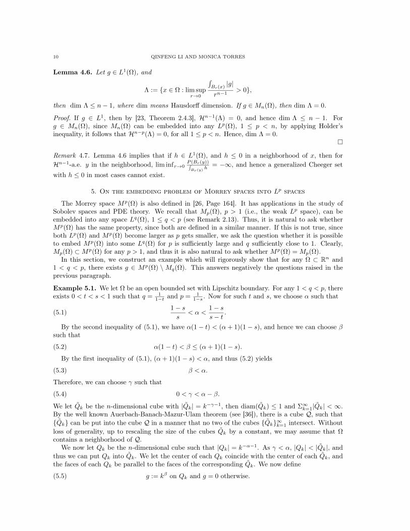
Lemma 4.6. Let g ∈ L1(Ω), and

Λ := x ∈ Ω : lim supr→0

´Br(x)

|g|rn−1

> 0,

then dim Λ ≤ n− 1, where dim means Hausdorff dimension. If g ∈Mn(Ω), then dim Λ = 0.

Proof. If g ∈ L1, then by [23, Theorem 2.4.3], Hn−1(Λ) = 0, and hence dim Λ ≤ n − 1. Forg ∈ Mn(Ω), since Mn(Ω) can be embedded into any Lp(Ω), 1 ≤ p < n, by applying Holder’sinequality, it follows that Hn−p(Λ) = 0, for all 1 ≤ p < n. Hence, dim Λ = 0.

Remark 4.7. Lemma 4.6 implies that if h ∈ L1(Ω), and h ≤ 0 in a neighborhood of x, then forHn−1-a.e. y in the neighborhood, lim infr→0

P (Br(y))´Br(y)

h= −∞, and hence a generalized Cheeger set

with h ≤ 0 in most cases cannot exist.

5. On the embedding problem of Morrey spaces into Lp spaces

The Morrey space Mp(Ω) is also defined in [26, Page 164]. It has applications in the study ofSobolev spaces and PDE theory. We recall that Mp(Ω), p > 1 (i.e., the weak Lp space), can beembedded into any space Lq(Ω), 1 ≤ q < p (see Remark 2.13). Thus, it is natural to ask whetherMp(Ω) has the same property, since both are defined in a similar manner. If this is not true, sinceboth Lp(Ω) and Mp(Ω) become larger as p gets smaller, we ask the question whether it is possibleto embed Mp(Ω) into some Lq(Ω) for p is sufficiently large and q sufficiently close to 1. Clearly,Mp(Ω) ⊂Mp(Ω) for any p > 1, and thus it is also natural to ask whether Mp(Ω) = Mp(Ω).

In this section, we construct an example which will rigorously show that for any Ω ⊂ Rn and1 < q < p, there exists g ∈ Mp(Ω) \Mq(Ω). This answers negatively the questions raised in theprevious paragraph.

Example 5.1. We let Ω be an open bounded set with Lipschitz boundary. For any 1 < q < p, thereexists 0 < t < s < 1 such that q = 1

1−t and p = 11−s . Now for such t and s, we choose α such that

(5.1)1− ss

< α <1− ss− t

.

By the second inequality of (5.1), we have α(1− t) < (α+ 1)(1− s), and hence we can choose βsuch that

(5.2) α(1− t) < β ≤ (α+ 1)(1− s).

By the first inequality of (5.1), (α+ 1)(1− s) < α, and thus (5.2) yields

(5.3) β < α.

Therefore, we can choose γ such that

(5.4) 0 < γ < α− β.

We let Qk be the n-dimensional cube with |Qk| = k−γ−1, then diam(Qk) ≤ 1 and Σ∞k=1|Qk| < ∞.By the well known Auerbach-Banach-Mazur-Ulam theorem (see [36]), there is a cube Q, such thatQk can be put into the cube Q in a manner that no two of the cubes Qk∞k=1 intersect. Withoutloss of generality, up to rescaling the size of the cubes Qk by a constant, we may assume that Ωcontains a neighborhood of Q.

We now let Qk be the n-dimensional cube such that |Qk| = k−α−1. As γ < α, |Qk| < |Qk|, andthus we can put Qk into Qk. We let the center of each Qk coincide with the center of each Qk, andthe faces of each Qk be parallel to the faces of the corresponding Qk. We now define

(5.5) g := kβ on Qk and g = 0 otherwise.


Clearly g is integrable, since ‖g‖L1(Ω) =∑k k

β−α−1 < ∞. We will show that for any cube Q,´Q∩Qk

|g||Q|s < ∞. Given any Q, we note that there are three possible situations. First, if Q does not

intersect any of the cubes Qk, then ´Q∩Ω|g|

|Q|s= 0.

Second, if Q ⊂ Qk for some k, then´Q∩Qk |g||Q|s

≤ kβ |Q ∩Qk||Q ∩Qk|s

= kβ |Q ∩Qk|1−s

≤ kβ |Qk|1−s

= kβ−(α+1)(1−s)

< ∞ , by the right half of (5.2).(5.6)

Finally, if Q is not contained in any of the cubes Qk, we let IQ = k : |Q∩Qk| > 0. For k ∈ IQ,by the geometry of Qk and Qk, there exists a universal constant C such that

(5.7)|Q ∩ Qk||Q ∩Qk|

≥ C k−γ−1

k−α−1= Ckα−γ .

Therefore ´Q∩Ω|g|

|Q|s≤

∑k∈IQ k

β |Q ∩Qk|(∑k∈IQ |Q ∩ Qk|)

s

≤ c

∑k∈IQ k

β |Q ∩Qk|(∑k∈IQ k

α−γ |Q ∩Qk|)s, c =

1

Cs, by (5.7)

≤ c

∑k∈IQ k

β |Q ∩Qk|(∑k∈IQ k

β |Q ∩Qk|)s, since α− γ > β

≤ c(∑k∈IQ

kβ |Q ∩Qk|)1−s

≤ c(∑k

kβ−α−1)1−s <∞(5.8)

Therefore, for any n-dimensional cube Q,´Q∩Ω|g|dx

|Q|1−1/p=

´Q∩Ω|g|

|Q|s< C(n) <∞.

That is,g ∈Mp(Ω).

However, let EK = ∪∞k=KQk´EK|g|

|EK |1−1q

=

´EK|g|

|EK |t

=Σ∞k=Kk

βk−α−1

(Σ∞k=Kk−α−1)t

∼ Kβ−α

K−αt

= Kβ−α(1−t)

→ ∞ as K →∞, by the first inequality of (5.2).(5.9)


Therefore, g /∈Mq(Ω).

Remark 5.2. Example 5.1 will also serve as a model example in the study of the critical caseg ∈Mn(Ω) in section 8.

6. on the regularity of generalized Cheeger sets for h ∈Mp(Ω), p > n.

In this section, we study the regularity of generalized Cheeger sets in an open bounded Lipschitzdomain Ω. A a generalized Cheeger set in Ω is a minimizer of the problem

(6.1) Ch0 := infF⊂Ω

Jh(F ), Jh(F ) =P (F )´Fhdx

, h nonnegative.

We recall that Ch0 = 1/v∗h1 .

Remark 6.1. From Remark 3.6 and Theorem 3.7 we see that, for n = 2, Ch0 > 0 if and only ifh ∈ M2(Ω), and for n ≥ 3 and Ω convex, Ch0 > 0 if and only if h ∈ S(Ω). Since S(Ω) ⊂ Mn(Ω) wesee that, in these cases, a necessary condition to guarantee the existence of generalized Cheeger setsin Ω is that h ∈Mn(Ω). This motivates our analysis with Morrey spaces.

We observe that, if the set of finite perimeter E minimizes Jh, that is, Jh(E) = Ch0 , then E isalso the minimizer of the restriction of the functional (2.2) to Ω, that is,

(6.2) IH(E) ≤ IH(F ) = P (F ) +

ˆF

H(x)dx, F ⊂ Ω,

where H(x) = −Ch0 h(x).Throughout the rest of the article we continue to assume that sptµE = ∂E (see [37, Remark 16.11

and Proposition 12.9]).We now state the first result concerning the regularity of generalized Cheeger sets.

Theorem 6.2. If Ω is a Lipschitz domain in Rn, h ∈ Mp(Ω), p > n, and Jh(E) = infF⊂Ω Jh(F ),

where Jh is defined as above, then Ω ∩ ∂∗E is a C1,α-hypersurface, where α = p−n2p . Moreover, the

singular set has dimension at most n− 8 (and it is empty if n ≤ 7).

Proof. Let Ch0 = infF⊂Ω Jh(F ). Clearly Ch0 > 0. We consider the functional IH(F ) = P (F ) +´

FH(x)dx with H = −Ch0 h(x). We note that IH is nonnegative and IH(E) = 0, and hence E is a

minimizer of IH . Moreover, H ∈Mp(Ω).Let F be a set such that E 4 F ⊂⊂ Br(x) ∩ Ω. By the minimality of E,

(6.3) P (E;Br(x)) +

ˆE∩Br(x)

H ≤ P (F ;Br(x)) +

ˆF∩Br(x)

H,

and using that H ∈Mp(Ω) we obtain

(6.4) P (E;Br(x)) ≤ P (F ;Br(x))+

ˆBr(x)

|H| ≤ P (F ;Br(x))+Crn−np = P (F ;Br(x))+Cr2αrn−1,

where C = ωn ‖H‖Mp(Ω) and 0 < α = p−n2p < 1

2 . It was shown in Tamanini [44] and Bombieri [15]that if a set E is a quasi minimizer in the sense that

(6.5) P (E;Br(x)) ≤ P (F ;Br(x)) + η(r)rn−1

for all variations F of the set E such that F 4 E ⊂⊂ Br(x) where η : (0, r0)→ [0,∞) satisfies

(6.6) η(0+) = 0,η(r)

ris increasing on (0, r0)

and

(6.7)ˆ r0

0

√η(r)

rdr <∞,


then ∂E can be split into the union of a C1 relatively open hypersurface and a closed singular setwith Hausdorff dimension at most n − 8 (empty if n ≤ 7). Moreover, given x ∈ ∂∗E, there existC, r > 0 such that

(6.8) |νE(x)− νE(y)| ≤ C

(ˆ |x−y|0

√η(r)

r+ |x− y|1/2

), for all y ∈ B(x, r) ∩ ∂∗E.

In our situation, from (6.4) it follows that our generalized Cheeger set E is a quasi minimizerin the sense of Tamanini (6.5) with η(r) ≤ cr2α. Moreover, we note that η satisfies the requiredconditions (6.6) and (6.7). Furthermore, from (6.8) we conclude that ∂E can be split into the unionof a C1,α relatively open hypersurface and a closed singular set with Hausdorff dimension at mostn− 8 (empty if n ≤ 7).

Corollary 4.4 immediately implies the following:

Theorem 6.3. If Ω is a Lipschitz domain in R2 and h ∈ Mp(Ω), p > 2, then infF⊂ΩP (F )´

Fh(x)dx

is

attained by a set E of finite perimeter. Moreover, Ω ∩ ∂E is a C1,α-hypersurface, where α = p−n2p .

Corollary 6.4. If h ∈ Lp(Ω), p > n, then infF⊂ΩP (F )´

Fh(x)dx

is attained by a set E of finite perimeter.Moreover, there exists a closed set Σ(E) with Hausdorff dimension not greater than n− 8 (empty ifn ≤ 7), such that (∂E ∩ Ω) \ Σ(E) is a C1, p−n2p (n− 1)-dimensional hypersurface.

Proof. That the infimum is attained by a set E ⊂ Ω follows from [12, Corollary 6.2], where theexistence for generalized Cheeger sets was proven for h ∈ Ln(Ω). The regularity follows from theclassical theory of variational mean curvatures (see, for example, Gonzalez-Massari [27] and thereferences therein) or from Theorem 6.2 since Lp(Ω) ⊂Mp(Ω).

Corollary 6.5. If h ∈ Ln(Ω), then generalized Cheeger sets E exist. Moreover, there exists a closedset Σ(E) with Hausdorff dimension not greater than n − 8, such that (∂E ∩ Ω) \ Σ(E) is a C0,α

(n − 1)-dimensional manifold for all α < 1. If n = 2, then ∂E ∩ Ω is a Lipschitz 1-dimensionalmanifold.

Proof. The existence follows from [12, Corollary 6.2]. The regularity for the critical case h ∈ Ln(Ω)was proven by Ambrosio-Paolini [6, Theorem 4.10, Theorem 5.2] (see also Paolini [41]).

We finish this section with a discussion about the critical case h ∈ Mn(Ω). Indeed, motivatedby the conjecture of De Giorgi discussed in the introduction (see Ambrosio-Paolini [6]) concerningthe regularity of boundaries with prescribed mean curvature in the critical space Ln, we would liketo know if the regularity in Corollary 6.5 holds for generalized Cheeger sets with h in the criticalspace Mn(Ω). We first note that a generalized Cheeger set is also a quasi minimizer in the sense ofAmbrosio-Paolini [6] since, from (6.5), it follows that

(6.9) P (E;Br(x)) ≤ (1 + ω(r))P (F ;Br(x)),

where ω(r) = c(n)r2α

1−c(n)r2α , α = n−p2p . However, for the critical case p = n, ω(r) becomes a constant

and hence the condition

(6.10) limr→0

ω(r) = 0

is not satisfied. Thus, we can not proceed as is [6], where this condition was critical to obtain theregularity described in Corollary 6.5. Indeed, the dimension estimates for the singularities of theminimizers in Corollary 6.5 depend heavily on the fact that, if h is Ln integrable, then the blow-uplimit E∞ is a minimal set with mean curvature H = 0 (see [28, Theorem 1.1]). Then, the dimensionestimates for the singularities follow from the non-existence of minimizing cones for n ≤ 7 andFederer’s dimension reduction argument (see, for example, [37, Chapter 28]). However, in order


to show that the blow-up limit has zero mean curvature, ω(r) must be infinitesimal, that is, thecondition w(0+) = 0 is needed.

The next Example 6.6 shows that the strong regularity described in Theorem 6.2 is not true ingeneral for the critical case h ∈Mn(Ω). We will show in Lemma 7.16 that our structure Theorem 7.7for generalized Cheeger sets implies upper density estimates on points of the boundary of generalizedCheeger sets. The following Example 6.6 also shows that the lower density bounds can fail forh ∈Mn(Ω). We will provide in Section 8 a stronger example (see Example 8.4), which shows that,even for h ∈ Mn(Ω) ⊂ Mn(Ω), the set of points where the lower density estimate fails can be verylarge.

Although Example 8.4 gives more information, Example 6.6 provides motivations for the proofof Theorem 7.7 and gives understanding about their behavior in the critical case h ∈Mn(Ω).

Example 6.6. This example is a continuation of Example 5.1. Let Ω be a bounded open setwith Lipschitz boundary and let n = 2. Let s = 1 − 1

n . Then, for any 1 < q < n, we canchoose 0 < t < s < 1 with t = 1 − 1

q . As in Example 5.1, we let 1−ss < α < 1−s

s−t and chooseβ = (α+ 1)(1− s) = α+1

n . Thus, we choose 0 < γ < α−β and define Qk and Qk as in Example 5.1.We now let

(6.11) h :=∑k

kβχCk ,

where Ck is the classical Cheeger set in Qk. Proceeding as in Example 5.1, h /∈Mq(Ω), h ∈Mn(Ω)and (5.7) holds.

Let CQ be the Cheeger constant of the unit cube. Thus, by scaling of perimeter and volume,

(6.12)P (Ck)

|Ck|= infF⊂Qk

P (F )

|F |=

CQl(Qk)

,

where the function l(Qk) denotes the length of the edge of the cube. Since l(Qk) = k−α+1n = k−β ,

we haveP (Ck)´Ckh

= k−βP (Ck)

|Ck|= k−β

CQl(Qk)

= CQ.

Let E =⋃k Ck, then

Jh(E) =

∑k P (Ck)∑k

´Ckh

= CQ.

For any indecomposable set F ⊂ E, by Theorem 2.8, F ⊂ Qk (mod Hn) for some k. Hence

(6.13)P (F )´Fh

= k−βP (F )

|F |≥ k−β P (Ck)

|Ck|= CQ.

For general F ⊂ E, let Fk be the indecomposable components of F . Hence Fk ⊂ E, P (Fk)|Fk| ≥ CQ,

and hence

Jh(F ) =

∑k P (Fk)∑k

´Fkh≥ CQ.

Therefore Jh(E) = infF⊂E Jh(F ). We now claim that E satisfies (7.6). Indeed, this is because each

Ck is convex (from which we can apply [37, Exercise 15.14]) and the distance between any two of thesets Ck is large compared to the diameter of each Ck, and hence, if ∂F connects two cubes Qi, Qj ,the part of ∂F whose projections to the direction of the edges of each Qk intersect Qk, but are notcontained in any cube Qk, has much larger length outside the union of the cubes Qk. The sameprojection argument as in [12, Example 7.3] can be used to verify this argument carefully. Therefore,since h ≥ 0 on E and h = 0 on Ec, Lemma 7.12 implies that this h and E satisfies (7.13). Hence,Proposition 7.10 imply that E satisfies (7.5), and thus E also satisfies (7.7). We have shown that Eis a generalized Cheeger set in Ω corresponding to the function h defined in (6.11).


We now proceed to show that the strong regularity of E fails by finding a point x0 ∈ ∂E ∩ E0.Let xk be the center of Qk. Since all the cubes Qk are contained in a cube Q ⊂⊂ Ω, we can findx0 such that, up to a subsequence, xk → x0. Clearly x0 ∈ spt ‖DχE‖ = ∂E. Let Qr be the cubecentered at x0 with edge lenght r. Then, for any r, by the geometry of Qk and Qk there exists auniversal constant C1 such that |Qr∩Qk||Qr∩Qk| ≥ C1k

α−γ (see (5.7)). Let I(r) = k : Qr ∩ Qk 6= ∅ andm(r) = inf I(r), then m(r)→∞ as r → 0. We have the following

|E ∩Br|rn

∼ |E ∩Qr||Qr|

=

∑k∈I(r) |Ck ∩Qr|

Σk∈I(r)|Qk ∩Qr|

≤ supk∈I(r)

|Ck ∩Qr||Qk ∩Qr|

< supk∈I(r)

|Qk ∩Qr||Qk ∩Qr|

≤ 1

C1m(r)γ−α → 0,(6.14)

which implies x ∈ E0. We conclude that E is a generalized Cheeger set in Ω corresponding to thecritical case h ∈Mn(Ω) for which the strong regularity fails.

7. structure of generalized Cheeger sets

The previous section was concerned with the differentiability properties of the boundaries ofgeneralized Cheeger sets. In this section, we are concerned about the shape of the sets, and inparticular their property of being pseudoconvex.

We recall that, for the variational mean curvature problem, given any set of finite perimeter E,there exists a function HE ∈ L1 such that E has mean curvature HE . Therefore, since sets offinite perimeter can have very rough boundaries, the same is true for minimizers of this problem.However, for the generalized Cheeger set problem, we will show in Theorem 7.7 that minimizershave the extra property of being pseudoconvex. Before stating the main result of this section, wemake some definitions:

Definition 7.1. Let Ω ⊂ Rn be a bounded open set with Lipschitz boundary or Ω = Rn, and letE ⊂ Ω be a bounded set of finite perimeter. We say that F is a set with least perimeter in Ωcontaining E if

(7.1) P (F ) = infP (F ) : Ω ⊃ F ⊃ E,

or, equivalentlyP (F ) ≤ P (F ), for all Ω ⊃ F ⊃ E.

Definition 7.2. A bounded set E ⊂ Rn of finite perimeter is called pseudoconvex if E is a set withleast perimeter in Rn containing E, that is

(7.2) P (E) = infP (F ) : Rn ⊃ F ⊃ E.

A pseudoconvex set E is also called a subsolution to the least area problem. If E ⊂ Rn is a boundedset of finite perimeter, then its minimal hull Em is defined as

Em =⋂

S∈JE

S,

where JE denotes the family of pseudoconvex sets in Rn that contain E.

Remark 7.3. From [8, Proposition 1.1], if each Ei, i = 1, 2, .., is a pseudoconvex set, then ∩iEi isalso a pseudoconvex set and, if in addition Ei ⊂ Ei+1, then ∪iEi is pseudoconvex. Hence, if E is aconvex set, then E is a pseudoconvex set (since a convex set is the intersection of hyperplanes). We


note that the disjoint union of two pseudoconvex sets is not necessarily pseudoconvex (consider forexample two disjoint parallel cubes sufficiently close to each other).

Remark 7.4. The previous remark implies that Em is a pseudoconvex set (see [10, Proposition 2.2])containing E and contained in the convex hull of E, E. Moreover, Em (see [10, Proposition 2.2]) isa set of least perimeter containing E, that is, (7.1) holds:

(7.3) P (Em) = minP (F ) : E ⊂ F,which implies

(7.4) P (Em) ≤ P (E) and P (Em) ≤ P (E).

We refer the reader to [24, Lemma 4] for the proof of the following theorem, which is very usefulin dealing with the case n = 2. This theorem is not true in higher dimensions, as shown in Remark7.6.

Theorem 7.5. Let E ⊂ R2 be an indecomposable bounded set. If E is not equivalent to a convexopen set, then there exists a bounded set F such that E ⊂ F and P (F ) < P (E).

7.1. Remark. Theorem 7.5 implies that E = Em in R2. Moreover, Em = E if and only if E is aconvex set.

Remark 7.6. We note that Theorem 7.5 is not true for n ≥ 3. In order to see this, we consider,in dimension 3, an open connected set E such that the perimeter of its convex hull E is strictlygreater than the perimeter of E. Such a set does not exists in dimension 2, but in dimension 3 onemay consider a set with the shape of a banana. We consider now the minimal hull Em of E. IfTheorem 7.5 were true in dimension 3 then Em would be convex, but if Em were convex then Emwould contain E and therefore [37, Exercise 15.14] and (7.4) would yield E = Em; that is,

P (E) = P (Em) ≤ P (E),

which contradicts that P (E) > P (E). Therefore, in dimension 3, when considering a set E withP (E) > P (E), the minimal hull Em is not convex.

In this section our main result is the following:

Theorem 7.7. (Structure Theorem)Let E be a bounded set of finite perimeter with |E| > 0. Then, E minimizes

(7.5) Jh(E) = infF⊂Rn

Jh(F ), Jh(F ) =P (F )´Fh(x)dx

for some h ∈ L1(Rn), h ≥ 0, if and only if E is pseudoconvex, that is,

(7.6) P (E) = infP (F ) : F ⊃ E.Moreover, if E is a minimizer for some Jh defined on Rn then, each indecomposable component Eiof E is also a minimizer for the same Jh and satisfies P (Ei) = infP (F ) : Ei ⊂ F. In particular,if n = 2, then Ei is H2-equivalent to a convex open set.

Remark 7.8. We recall that a set E satisfying (7.5) is called a generalized Cheeger set.

If instead we consider our problem in a bounded Lipschitz domain Ω, we similarly have

Theorem 7.9. Let E ⊂ Ω be a set of finite perimeter with |E| > 0, where Ω is a bounded Lipschitzdomain. Then, E minimizes

(7.7) Jh(E) = infF⊂Ω

Jh(F ), Jh(F ) =P (F )´Fh(x)dx

for some h ∈ L1(Ω), h ≥ 0, if and only if E satisfies

(7.8) P (E) = infP (F ) : Ω ⊃ F ⊃ E.


Moreover, if E is a minimizer for some Jh defined on Ω then, each indecomposable component Eiof E also minimizes the same Jh and satisfies P (Ei) = infP (F ) : Ω ⊃ F ⊃ Ei. In particular, ifΩ is convex and n = 2, then Ei is H2-equivalent to a convex open set.

In order to prove Theorem 7.7, we need some preliminary results.

Proposition 7.10. Let Jh be defined as in (7.5). If Jh(E) ≤ Jh(F ) for either F ⊂ E or F ⊃ E,then Jh(E) = infF⊂Rn J

h(F ).

Proof. We let F be any set of finite perimeter. Using that E is a minimizer of (7.7) and thehypothesis, it follows that

P (E)Éh(x)dx

≤ min

P (E ∩ F )É∩F h(x)dx

,P (E ∪ F )É∪F h(x)dx

≤ P (E ∩ F ) + P (E ∪ F )´

E∩F h(x)dx+É∪F h(x)dx

=P (E ∩ F ) + P (E ∪ F )Éh(x)dx+

´Fh(x)dx

.(7.9)

By the well known inequality (see [4, Proposition 1, Section 1])

(7.10) P (E ∩ F ) + P (E ∪ F ) ≤ P (E) + P (F )

we haveP (E)Éh(x)dx

≤ P (E) + P (F )Éh(x)dx+

´Fh(x)dx

.

Therefore,P (E)Éh(x)dx

≤ P (F )´Fh(x)dx

which yields Jh(E) = infF Jh(F ).

Lemma 7.11. For 0 < |E| < ∞, E a set of finite perimeter, if h = −HEχE where HE is as inTheorem 2.7, and χE is the characteristic function of E, then the following is true:

(7.11) Jh(E) = infF⊂E

Jh(F )

Proof. From Theorem 2.7, HE < 0 a.e. on E, and thus h > 0 a.e. on E. Also, from Theorem 2.7,

infF⊂Rn

IHE (F ) = IHE (E) = P (E) +

Ê

HE = P (E)− ‖HE‖L1(E) = 0.

Hence, in particular,

(7.12) P (F ) +

ˆF

HE(x)dx ≥ 0, for any F ⊂ Ω.

If F ⊂ E and F is not equivalent to the empty set, then´Fh(x)dx =

´F

(−HE(x))dx > 0, and(7.12) yields

P (F )´Fh(x)dx

=P (F )´

F(−HE(x))dx

≥ 1 =P (E)

‖HE‖L1(E)

=P (E)Éh(x)dx

This finishes the proof.

Lemma 7.12. Let E ⊂ Rn is a bounded set of finite perimeter. If there exists h ∈ L1(Rn), h ≥ 0a.e., such that

(7.13) Jh(E) = infRn⊃F⊃E

Jh(F ).

then E satisfies condition (7.6). Conversely, if E satisfies condition (7.6), then (7.13) is true forany h ∈ L1(Rn), h ≥ 0 a.e. on E and h = 0 on Ec.


Proof. If (7.13) is true, then for any F ⊃ E,

P (E)Éh(x)dx

≤ P (F )´Fh(x)dx

≤ P (F )Éh(x)dx

, sinceÊ

h(x)dx ≤ˆF

h(x)dx.(7.14)

Therefore, P (E) ≤ P (F ) and (7.6) is verified.If E satisfies (7.6), we now show that E satisfies (7.13) for any nontrivial h ≥ 0, h ∈ L1(Rn) and

h ≡ 0 on Ec. Indeed, for any such h we clearly haveÉh(x)dx =

´Fh(x)dx for F ⊃ E. Therefore,

for any F ⊃ E, we have

P (F )´Fh(x)dx

=P (F )Éh(x)dx

≥ P (E)Éh(x)dx

, by (7.6),

which finishes the proof of (7.13).

We are now ready to give the proof of Theorem 7.7.

Proof of Theorem 7.7. :If (7.5) is true, then (7.13) is clearly true. By Lemma 7.12, (7.6) is verified. If (7.6) is true, we

choose h = −HEχE , with HE defined as in Theorem 2.7. By Lemma 7.11, (7.11) is satisfied. Sinceh = 0 on Ec, Lemma 7.12 shows that (7.13) is true. Hence, by Proposition 7.10, (7.5) is verified andthus we finished the proof.

It remains to show that if E satisfies the condition (7.5), then each indecomposable componentEi of E also satisfies condition (7.5). Indeed, by the minimality of E and Theorem 2.8, we have thefollowing

(7.15)P (E)Éh≤ inf

i

P (Ei)Éih≤∑i P (Ei)∑i

Éih

=P (E)Éh.

One easily see that "=" holds if and only if

(7.16)P (Ei)Éih

=P (E)Éh, ∀i.

Therefore for any i, Ei also minimizes Jh, that is, Ei satisfies (7.5). This finishes the proof.

We note that the proof of Theorem 7.9 is analogous to the proof of Theorem 7.7, with the onlyextra task of showing that, if Ω is convex and E ⊂ Ω ⊂ R2 is indecomposable and satisfies (7.8),then E is equivalent to a convex open set. Indeed, if E is not convex, by Theorem 7.5, there existsa set of finite perimeter F such that F ⊃ E and P (F ) < P (E). Since Ω is convex, [37, Exercise15.14] gives P (F ∩Ω) ≤ P (F ), and thus P (F ∩Ω) < P (E). But Ω ⊃ F ∩Ω ⊃ E, and hence (7.8) isnot satisfied, which gives a contradiction.

We have the following:

Proposition 7.13. If each Ei, i = 1, 2, ..., minimizes Jh in Ω, then ∪iEi and ∩iEi (if not Hn-equivalent to the empty set) also minimizes Jh in Ω. As a direct consequence, there exists a uniquemaximal generalized Cheeger set.


Proof. Let E and F be generalized Cheeger set for Jh in Ω, then by (7.10), we have

P (E)Éh(x)dx

=P (F )´Fh(x)dx

≤ min

P (E ∩ F )É∩F h(x)dx

,P (E ∪ F )É∪F h(x)dx

≤ P (E ∩ F ) + P (E ∪ F )´

E∩F h(x)dx+É∪F h(x)dx

≤ P (E) + P (F )Éh(x)dx+

´Fh(x)dx

=P (E)Éh(x)dx

.

Therefore,P (E ∪ F )É∪F h(x)dx

=P (E ∩ F )É∩F h(x)dx

(if |E ∩ F | > 0) =P (E)Éh(x)dx

,

and hence E ∪ F and E ∩ F (if |E ∩ F | > 0) are generalized Cheeger set for h. By induction,generalized Cheeger sets are closed under finite unions and finite intersections (if not equivalent tothe empty set). By the lower semicontinuity property of sets of finite perimeter, this is also true forcountable unions or countable intersections (if not equivalent to the empty set).

Immediately from the proof of Theorem 7.7 and Proposition 7.13, we have the following:

Corollary 7.14. If E is a generalized Cheeger set in Rn (Ω resp.) for some h, then the union ofany subcollection of its indecomposable components is still a generalized Cheeger set for the same h,that is, such union satisfies condition (7.5) ( (7.7) resp.).

Remark 7.15. Let n = 2 and E be an indecomposable minimizer for (7.7). If Ω is only a Lipschitzdomain, it is not difficult to find an example (for instance, let Ω be a glove-like picture with a bighole), such that E is not convex. Even if we choose a ball B ⊂ Ω nontrivially intersecting E, E ∩Bmay not be equivalent to a convex open set. However, if Ω is a simply connected, n = 2 and E isan indecomposable subset of Ω satisfying (7.7) then, for any convex open subset K of Ω nontriviallyintersecting E, we claim that K ∩ E is equivalent to a convex open set. The proof of this claimfollows as in [24, Theorem 1]. The only difference is that we cannot directly apply [24, Lemma 4]because the set with least perimeter containing E might not be contained in Ω. In order to solvethis problem we argue as follows. Since Ω is simply connected, by [4, Corollary 1] we can assumeE = int C+ where C+ is a rectifiable Jordan curve. If our claim were false, then we could finda, b ∈ C+ such that the segment (a, b) is contained in Ω but also in the exterior of C+. Applying thesame argument as in the proof of [24, Lemma 4], we could find Γ1,Γ2 and F such that C+ = Γ1∪Γ2,F = int (Γ1∪ [a, b]), E ⊂ F and P (E) > P (F ). Since Ω is simply connected and Γ∪ [a, b] is a Jordancurve, the Jordan Curve Theorem yields F ⊂ Ω, and thus we obtain a contradiction to (7.8).

The following corollary gives upper density estimates at points in the boundary of generalizedCheeger sets.

Corollary 7.16. If E minimizes Jh in Ω and x ∈ ∂E, then there exists c1(n) and c2(n) such that

P (E;Br(x))

rn−1≤ c1(n), and

|E ∩Br(x)|rn

≤ c2(n)

hold for every Br(x) ⊂⊂ Ω.

Proof. We compare E with E ∪Br(x) and use Theorem 7.9 to deduce P (E) ≤ P (E ∪Br(x)). Since,for a.e. r > 0, Hn−1(∂∗E ∩ ∂Br) = 0, from [37, Theorem 16.3] we have

(7.17) P (E;Br(x)) ≤ Hn−1(E0 ∩ ∂Br).This proves the first inequality.

Adding Hn−1(E0 ∩ ∂Br) on both sides of (7.17), we have

P (E \Br(x)) ≤ 2Hn−1(E0 ∩ ∂Br).Let g(r) = |E \ Br(x)|, then g′(r) = Hn−1(E0 ∩ ∂Br) for a.e. r > 0. Hence, the isoperimetricinequality yields C(n)g(r)

n−1n ≤ 2g′(r), and this implies the upper density estimate for |E∩Br(x)|

rn .


8. The critical case h ∈Mn(Ω)

We now recall the notion of pseudoconvex set (see Definition 7.2). In this section we give anexample of a pseudoconvex set E and h ∈ Mn (i.e. the weak Ln space) such that E minimizes Jhbut |∂E ∩ E0| > 0. That is, the strong regularity described in section 6 fails in this critical case.

The result in Corollary 7.14, which is a direct consequence of Theorem 7.7, is stated in thelanguage of pseudoconvex sets in the following:

Theorem 8.1. Any countable union of indecomposable components of a pseudoconvex set is alsopseudoconvex, and in particular each indecomposable component of a pseudoconvex set is still pseu-doconvex.

As a direct consequence, we have the following result:

Corollary 8.2. For any set of finite perimeter E, there exists a countable family Fi of disjoint,indecomposable and pseudoconvex sets such that

E ⊂ ∪iFi (mod Hn) and∑i

P (Fi) ≤ P (E).

Proof. Given E, we consider its minimal hull Em. We let Fi be the indecomposable componentsof Em. Then, by Theorem 8.1, each Fi is pseudoconvex and hence Theorem 2.8 and Remark 7.4yield

P (E) ≥ P (Em) =∑k

P (Fi),

from which the corollary is proved.

Lemma 8.3. Let xj ⊂ Rn be a sequence of points in Rn and let ρj be a decreasing sequence ofpositive numbers in such a way that

(i) ∑j

ρj ≤ 1

(ii)Bρj (xj) ∩Bρi(xi) = ∅ for all j 6= i.

Then there exists a sequence rj such that for any 0 < sj < rj,

G = ∪jBsj (xj)is a pseudoconvex set.

Proof. Choose a fixed number q ≥ 4 large enough such that

nwn∑j≥1

(1

qn−1

)j<wn−1

4n−1.

Let rj =ρjqj . For any sj < rj , let

G =

∞⋃j=1

Bsj (xj).

From Proposition 7.13, in order to show that G is pseudoconvex it is enough to prove that, for everym = 1, 2, .., the set

Gm =

m⋃j=1

Bsj (xj)

is a pseudoconvex set. If suffices to show if F is a set with least perimeter containing Gm (seeDefinition 7.1), then F = Gm. To show this, it suffices to show the set J := j : ∂F∩∂Bρj/2(xj) 6= ∅is empty. Indeed, if so, then by the minimum property of F and the pseudoconvexity of Bsj (xj), it


follows that one of the following situations can occur:(i): F ∩B ρj

2(xj) = Bsj (xj),

(ii): B ρj2

(xj) ⊂ F .We let J1 = j ∈ 1, ..,m : F ∩B ρj

2(xj) = Bsj (xj) and define

F1 = F \ (∪j∈J1Bsj (xj)).

It suffices to show that F1 = ∅. We note from (ii) that dist(∂F1,∪j /∈J1

Bsj (xj))> δ > 0. We let

F = ∪j∈J1Bsj (xj) ∪ λF1, where λ < 1. For λ close enough to 1 we have that G ⊂ F and

P (F ) = P (∪j∈J1Bsj (xj)) + P (λF1) = P (∪j∈J1

Bsj (xj)) + λn−1P (F1) < P (∪j∈J1Bsj (xj)) + P (F1)

= P (F ),

which contradicts the minimality of F . Thus, we conclude that F1 = ∅. Hence Gm = F and thusGm is pseudoconvex.

Now we are left to prove J = ∅. If there exists a point yj ∈ ∂F ∩∂B ρj2

(xj) then, the lower densityestimate for perimeter minimizers (see for example [37, Section 17.4]) gives P (F ;Cj) ≥ wn−1(

ρj4 )n−1,

with Cj = Bρj (xj) \Bsj (xj). Let α ≥ 1 be the smallest number in J . We have, by the choice of q,

P (Gm)− P (F ) ≤∑j≥α

nwnsn−1j − wn−1

(ρα4

)n−1

,

≤∑j≥α

nwn

(ρjqj

)n−1

− wn−1

(ρα4

)n−1

≤ ρn−1α

nwn∑j≥α

(1

qn−1

)j− wn−1

4n−1

< 0,(8.1)

and thus we get a contradiction to the minimality of F . Therefore, J = ∅.

We can now give the main example in this section. We are motivated by the question of estimatingthe size of the points with density zero on the boundary of a generalized Cheeger set. By Theorem8.1, each indecomposable component of E is also pseudoconvex. Since a ball is convex, and thuspseduconvex, hence a starting point is to show the existence of a sequence of disjoint balls Bi suchthat ∂(∪iBi) \∪i(∂Bi) has Hausdorff dimension larger than n− 1. We will accomplish this by usinga classical Cantor-like set, Cα, which is nowhere dense and has positive measure α. Then, following[8, Section 3], where a pseudoconvex set with |∂E| > 0 was constructed, we will show the existenceof a pseudoconvex set E with |∂E ∩ E0| > 0.

Although Example 8.4 is written for the case n = 2, a similar construction in higher dimensionscan be done.

Example 8.4. This example uses the the classical construction of a Cantor-type set Cα ⊂ [0, 1]with positive measure 0 < α < 1. At each step m = 1, 2, 3, .., let Ami, i = 1, 2, ..., 2m−1, be the openintervals removed in the m-th step, with length 1−α

3m , and let Imk, k = 1, 2, ..., 2m, be the remainingdisjoint closed intervals in the m-th step. Let Cα = ∩∞m=1∪2m

k=1 Imk, where Cα is the classical Cantor-type set with measure α. Denote by ami, bmk the centers of the intervals Ami, i = 1, 2, ..., 2m−1,and Imk, k = 1, 2, ..., 2m, respectively. Let Qm = (ami, bmk), (bmk, ami), i = 1, 2, ..., 2m−1, k =1, 2, ..., 2m and let D = ∪∞m=1Qm = xj : j ∈ N.

Clearly by the construction, Cα × Cα ⊂ D. We can choose ρj small enough such that the ballsBρj (xj) are pairwise disjoint. We now choose sj satisfying Lemma 8.3 and

(8.2) sj+1 ≤1

2sj ,


(8.3)sjρj→ 0

and

(8.4)∑j

|Bsj (xj)| < α2 = |Cα × Cα| ≤ |D|.

LetE = ∪jBsj (xj)

and hence by Lemma 8.3 and (8.4), E is pseudoconvex and |∂D \ E| > 0. Clearly,

(8.5) ∂D \ E ⊂ ∂EWe note that the construction above also holds for any dimension n, so we use n instead of 2 in

following calculation.For any ball B intersecting both Bρj (xj) and Bsj (xj), there exists a universal constant C (i.e., it

does not depend on B and j), such that

(8.6)|B ∩Bsj (xj)||B ∩Bρj (xj)|

≤ C(sjρj

)n→ 0, as j →∞,

For any x ∈ ∂D \ E, we will follow as in Example 6.6 to show that x ∈ E0, and hence (8.5) implies|∂E ∩ E0| > 0.

Indeed, let Br be the ball centered at x, then as long as Br intersect some Bsk(xk), Br intersectBρk(xk). Let I(r) = k : Br ∩ Bsk(xk) 6= ∅ and m(r) = inf I(r), then m(r) → ∞ as r → 0. Wehave the following

|E ∩Br|rn

∼ |E ∩Br||Br|

≤∑k∈I(r) |Br ∩Bsk(xk)|

Σk∈I(r)|Br ∩Bρk(xk)|

≤ supk∈I(r)

|Br ∩Bsk(xk)||Br ∩Bρk(xk)|

→ 0, since m(r)→∞ and (8.6)

We now let

(8.7) h =∑k

1

skχBsk (xk),

and note that this function is supported on E. Since E is pseudoconvex then (7.6) holds andthus Theorem 7.7 implies that E is a generalized Cheeger set in Rn for some h ∈ L1(Rn), h ≥ 0.Proceeding as in Example 6.6, it follows that E is also a generalized Cheeger set corresponding thefunction h defined in (8.7). Clearly, E is also a generalized Cheeger set in any bounded open setwith Lipschitz boundary Ω that contains [0, 1]× [0, 1]. We will show that

h ∈Mn(Ω).

Since Mn(Ω) = Ln,w(Ω), we need to show that tn||h| > t| is bounded uniformly for t large (sinceΩ has finite measure). Indeed, for any t large, there exist sk such that

1

sk< t ≤ 1

sk+1,

and hence by the definition of h and (8.2),

tn||h| > t| ≤ 1

snk+1

∣∣∣∣h > 1

sk

∣∣∣∣ =1

snk+1

∑i≥k+1

nwnsni ≤ nwn

1

snk+1

snk+1

1− ( 12 )n≤ 2nwn.

The previous example shows the following:


Theorem 8.5. For any open bounded set Ω with Lipschitz boundary, there exists a generalizedCheeger set E ⊂ Ω, corresponding to h ∈ Mn(Ω) ⊂ Mn(Ω), such that |∂E ∩ E0| > 0. Hence, thestrong regularity fails in the critical case h ∈Mn(Ω).

9. An application to averaged shape optimization

In Bright-Li-Torres [12], we considered the following averaged shape optimization problem

(9.1) v∗2 = infE⊂Ω

V2(E), V2(E) =

´∂∗E

f(x,νE(x))dHn−1(x)

Hn−1(∂∗E),

which includes, for example, the minimization of the averaged flux of a physical quantity in the casef(x,νE(x)) = F · νE .

The averaged nature of V2(E) in (9.1) allows for the optimal value v∗2 = infE⊂Ω V2(E) to beapproximated by a sequence of sets Ei with P (Ei)→∞ or |Ei| → 0. In the former case we cannotapply the compactness theorem for sets of finite perimeter, and for the latter case the limit of theminimizing sequence degenerates. Also, due to the averaged nature of the problem, we can not guar-antee that the functional V2(E) is lower semicontinuous. The study of these degenerated cases wasinitiated in Bright-Torres [13] and continued in Bright-Li-Torres [12]. The nonlinear problem (9.1)was transformed into a linear problem in [12] by introducing the concept of occupational measures(see [12, Definition 2.5]) and the atomic value of V2 (see [12, see Section 4]). The perturbation of(9.1) with a Cheeger term:

(9.2) v∗ = infE⊂Ω

V (E), V (E) =

´∂∗E


Hn−1(∂∗E)= V2(E) + V g1 (E),

was studied in Bright-Li-Torres [12], under the condition that g ∈ Ln(Ω). In this section we willshow that the main results in [12] remains true, for n = 2, if g belongs to the Morrey spaces Mp(Ω),p > 2.

We first recall (see [12, Definition 2.5]) and [12, see Section 4]) the following definitions:

Definition 9.1. We define the atomic value of the minimization problem v∗2 = infE⊂Ω V2(E) at thepoint x0 ∈ Ω as

(9.3) fatom (x0) = infµ∈P0(Sn−1)

ˆSn−1

f (x0, v) dµ (v) ,

where

(9.4) P0

(Sn−1

)=

µ ∈ P

(Sn−1

):

ˆSn−1

vdµ (v) = 0 ∈ Rn.

The atomic value of the problem is

(9.5) fatom = minx0∈Ω

fatom(x0)

We recall the definitions of the spaces S(Ω) and Sc(Ω) introduced in section 5. We have thefollowing:

Theorem 9.2. Consider the minimization problem v∗ = infE⊂Ω V (E) given by

(9.6) V (E) =

´∂∗E


Hn−1(∂∗E)= V2(E) + V g1 (E)

where f ∈ C(Ω× Sn−1).(a) If g ∈ Sc(Ω) then, for every point x0 ∈ Ω, the atomic value at x0, fatom (x0), can be realized

by a sequence of convex polytopes ∆i ⊂ Ω with n+ 1 faces shrinking to x0, in the sense that

limi→∞

supy∈∆i

|y − x0| = 0,


and such thatlimi→∞

V (∆i) = fatom (x0) .

More precisely, v∗ ≤ fatom.(b) If g ∈ S(Ω) then, if there exists a minimizing sequence Ei such that P (Ei)→∞ or P (Ei)→ 0,

then v∗ ≥ fatom. In this case, from (a), v∗ = fatom and v∗ can be approximated by convex polytopes∆i with n+ 1 faces shrinking to a point x0.

Remark 9.3. Since ∆i are convex, limi→∞ supy∈∆i|y − x0| = 0 actually implies that P (∆i)→ 0.

Proof of Theorem 9.2. Given x0 ∈ Ω, let ∆i be the sequence of convex polytopes constructed in[12, Proposition 4.9]. Notice that [12, Equality (4.9)] yields

(9.7) V2(∆i)→ fatom(x0),

By remark 9.3, since g ∈ Sc(Ω), we have that limi→∞ V g1 (∆i) = 0, and hence

(9.8) limi→∞

V (∆i) = fatom(x0).

Since fatom = fatom(x0), for some x0 ∈ Ω, we have that v∗ ≤ fatom, which is (a).

For (b), if Ei is a minimizing sequence of (9.9) such that P (Ei) → ∞ then´Eigdx

Hn−1(∂∗Ei)→ 0

and hence V g1 (Ei) → 0. Also, if limi→∞ P (Ei) = 0, the assumption g ∈ S(Ω) implies again thatV g1 (Ei) → 0. Since P (Ei) → 0 implies |Ei| → 0, hence the condition of [12, Theorem 2.16] issatisfied. Let µ1, µ2, · · · ∈ P

(Ω× Sn−1

)be the corresponding sequence of occupational measures.

By compactness there exists a subsequence, denoted again as the full sequence, such that µi∗ µ0 ∈

P(Ω× Sn−1

). Note that µ0 is not necessarily an occupational measure corresponding to a set of

finite perimeter. Hence, using [12, property (2.4) of occupational measures],

v∗ = limi→∞

1

P (Ei)

ˆ∂∗Ei

f(x,νEi(x))dHn−1(x) + 0, since V g1 (Ei)→ 0,

= limi→∞

ˆΩ×Sn−1

f (x, v) dµi =

ˆΩ×Sn−1

f (x, v) dµ0 =

ˆΩ

(ˆSn−1

f (x, v) dµx0

)dp0,

where µ0 = p0~µx0 is the disintegration of the measure µ0. By [12, Theorem 2.16], µx0 ∈ P0

(Sn−1

),

for p0-almost every x. Then, Definition 9.1 implies that the inner integral is bounded from belowby fatom, and, since p0

(Ω)

= µ0

(Ω× Sn−1

)= 1, fatom ≤ v∗.

From Theorem 4.3 and Theorem 9.2 we conclude with the following:

Corollary 9.4. Consider the minimization problem v∗ = infE⊂Ω V (E) given by

(9.9) V (E) =

´∂∗E


Hn−1(∂∗E)= V2(E) + V g1 (E)

where f ∈ C(Ω× Sn−1). If g ∈ Mp(Ω), p > n, then, if there exists a minimizing sequence Ei suchthat P (Ei) → ∞ or P (Ei) → 0, then v∗ = fatom and v∗ can be approximated by convex polytopes∆i with n+ 1 faces shrinking to a point x0.

Remark 9.5. We note that both Corollary 9.4 and Corollary 4.4 truly generalize the main approx-imation result in [12, Theorem 5.3] and the existence result in [12, Corollary 6.2] since the spacesMp(Ω), p > n, are not contained in Ln(Ω). Indeed, we have shown in Section 4 that Mp(Ω), p > n,can not be embbeded into the weak Ln(Ω) space, Mn(Ω), which contains Ln(Ω).

Acknowledgement

The authors would like to thank Elisabetta Barozzi, Nicola Fusco and Changyou Wang for usefulcomments.


References

[1] A. D. Alexandrov. Convex Polyhedra. Springer-Verlag, Berlin, 2005. Monographs in Mathematics. Translationof the 1950 Russian edition by N. S. Dairbekov, S. S. Kutateladze, and A. B. Sossinsky.

[2] F. Alter and V. Caselles. Uniqueness of the Cheeger set of a convex body. Nonlinear Analysis, 70(1):32-44, 2009.[3] F. Alter, V. Caselles and A. Chambolle. A characterization of Convex Calibrable Sets in Rn. Mathematische

Annalen, 332:329-366, 2005.[4] L. Ambrosio, V. Caselles, S. Masnou and J.M. Morel. Connected components of sets of finite perimeter and

applications to image processing. Journal of the European Mathematical Society, 3(1): 39–92,2001.[5] L. Ambrosio, N. Fusco, and D. Pallara. Functions of Bounded Variation and Free Discontinuity Problems. Oxford

Mathematical Monographs. The Clarendon Press, Oxford University Press: New York, 2000.[6] L. Ambrosio and E. Paolini. Partial regularity for quasi minimizers of perimeter Ricerche Mat., 48:167-186,1999.[7] Z. Artstein and I. Bright. Periodic optimization suffices for infinite horizon planar optimal control. SIAM J.

Control Optim., 48:4963–4986, 2010.[8] E. Barozzi, E. Gonzalez and U. Massari. Pseudoconvex sets. Ann.Univ.Ferrara., 55:23-35, 2009.[9] E. Barozzi, E. Gonzalez and I. Tamanini. The mean curvature of a set of finite perimeter. Proceedings of the

American mathematical society, 99(2):313-316, 1987.[10] R.C. Bassanezi and I. Tamanini. Subsolutions to the Least Area Problem and the Minimal Hull of a Bounded

Set in Rn. Ann. Univ. Ferrara. Sez.VII-Sc.Mat., Vol.XXX: 27-40, 1984.[11] P. Billingsley. Convergence of probability measures. Wiley-Interscience, 2009.[12] I. Bright, Q. Li and Monica Torres. Occupational measures and averaged shape optimization Submitted,

www.math.purdue.edu/∼torres, 2016.[13] I. Bright and M. Torres. The integral of the normal and fluxes over sets of finite perimeter. Interfaces and free

boundaries, 17, 245-259, 2015.[14] G. Butazzo, G. Carlier and M. Comte. On the selection of maximal Cheeger sets. Differential Integral Equations,

20(9):991-1004, 2007.[15] E. Bombieri. Regularity theory for almost minimal currents. Arch. Rational Mech. Anal. 78 (1982), 99-130.[16] G. Carlier, M. Comte and G. Peyré. Approximation of maximal Cheeger sets by projection. Math. Model. Number

Anal., 43(1):139-150, 2008.[17] G. Carlier and M. Comte. On a weighted total variation minimization problem. J. Funct. Anal., 250:214-226,

2008.[18] V. Caselles, A. Chambolle and M. Novaga. Uniqueness of the Cheeger set of a convex body. Pacific Journal of

Mathematics, 231(1):77-90, 2007.[19] V. Caselles, A. Chambolle and M. Novaga. Some Remarks on uniqueness and regularity of Cheeger sets. Rend.

Sem. Mat. Univ. Padova, 123, 2010.[20] J. Cheeger. A lower bound for the smallest eigenvalue of the Laplacian. Problems in analysis, Princeton Univ.

Press, New Jersey, 195-199, 1970.[21] Su una teoria generale della misura (r − 1)-dimensionale in uno spazio a r dimensioni, Ann.Mat.Pura Appl. Ser

IV 36(1954),191-213[22] Frontiere orientate di misura minima, Seminario di Matmatica della Scuola Normale Superiore di Pisa, Editrice

Tecnico Scientifica, Pisa, 1961.[23] C. Evans and D. Gariepy. Measure Theory and Fine Properties of Functions. CRC Press, Boca Raton, FL, 1992.[24] A. Ferriero and N. Fusco. A note on the convex hull of sets of finite perimeter in the plane, discrete and continuous

dynamical systems series B, Volume 11, Number 1, January 2009.[25] A. Figalli, F. Maggi and A. Pratelli. A note on Cheeger sets. Proc. Amer. Math. Soc., 137, 2057-2062, 2009.[26] David Gilbarg and Neil S. Trudinger. Elliptic partial differential equations of second order, Second edition.

Springer-Verlag, Berlin, 1983.[27] E. Gonzalez and U. Massari. Variational mean curvatures. Rend. Sem. Mat. Univ. Pol. Torino, 52(1):1-28,

1994.[28] E. Gonzalez, U. Massari and I. Tamanini. Boundaries of prescribed mean curvature. Rend. Mat. Acc. Lincei,

4(3):197-206, 1993.[29] Loukas Grafakos. Classical Fourier Analysis, Second Edition, Graduate Texts in Mathematics, 249. Springer,

New York, 2008.[30] P. Gruber. Convex and discrete geometry. Springer, 2007.[31] W. Gustin. Boxing inequalities. J. Math. Mech., 9:229-239, 1960.[32] I. R. Ionescu and T. Lachand-Robert. Generalized Cheeger sets related to landslides, Calculus of Variations and

Partial Differential Equations, 23(2):227–249, 2005.[33] B. Kawohl and V. Fridman. Isoperimetric estimates for the first eigenvaluable of the p-Laplace operator and the

Cheeger constant. Comment. Math. Univ. Carolin., 44:659-667, 2003[34] B. Kawohl and T. Lachand-Robert. Characterization of Cheeger sets for convex subsets of the plane. Pacific J.

Math., 225:103-118, 2006


[35] B. Kawohl and M. Novaga. The p-Laplace eigenvalue problem as p→ 1 and Cheeger sets in a Finsler metric, toappear on J. Convex Analysis.

[36] A. Kosinski, A proof of an Auerbach-Banach-Mazur-Ulam theorem on convex bodies. Colloq.Math., 17(1957),216-218.

[37] F. Maggi Sets of finite perimeter and geometric variational problems Cambridge, 2011.[38] Umberto Massari. Esistenza e regolarit à delle ipersuperfice di curvatura media assegnata in Rn. Arch. Rational

Mech. Anal.,55:357-382, 1974.[39] Umberto Massari. Frontiere orientate di curvatura media assegnata in Lp. Rend. Sem. Mat. Univ. Padova,

53:37-52, 1975.[40] C.B. Morrey. On the solutions of quasi-linear elliptic partial differential equations. Trans. Amer. Math. Soc.,

1:126-166, 1938.[41] Paolini. Regularity for minimal boundaries in Rn with mean curvature in Ln, manuscripta math. 97,15-35(1998).[42] E. Parini. An introduction to the Cheeger problem. Surveys in Mathematics and its Applications, 6:9-22, 2011.[43] H. Rafeiro, N. Samko and S. Samko. Morrey-Campanato spaces: an overview. (English summary) Opera-

tor theory, pseudo-differential equations, and mathematical physics, 293–323, Oper. Theory Adv. Appl., 228,Birkhuser/Springer Basel AG, Basel, 2013.

[44] I. Tamanini. Regularity Results for Almost Minimal Oriented Hypersurfaces in RN . Quaderni del Dipartimentodi Matematica dell’Universit à di Lecce. Lecce, Universit à di Lecce, 1984.

[45] W.P. Ziemer. Weakly Differentiable Functions, Graduate Texts in Mathematics. Springer-Verlag: New York,120, 1989.

[Q. Li] Department of Applied Mathematics, Purdue University,E-mail address: [email protected]

[M. Torres]Department of Mathematics, Purdue University, 150 N. University Street, West Layayette,IN 47907-2067, USA. http://www.math.purdue.edu/˜torres

E-mail address: [email protected]

morrey spaces and generalized cheeger sets

Documents