morpheus et al. - florida state...
TRANSCRIPT
Morpheus et al.Java Edition
(Revision: 20140704)
User's GuideDennis E. Slice
Morpheus et al., Java Edition
Program revision: 20140704Document version: June 29, 2014
Author: Dennis E. SliceDepartment of Scientific ComputingThe Florida State UniversityTallahassee, Florida, USA 32306
andDepartment of AnthropologyUniversity of ViennaVienna, Austria
Contact: [email protected]
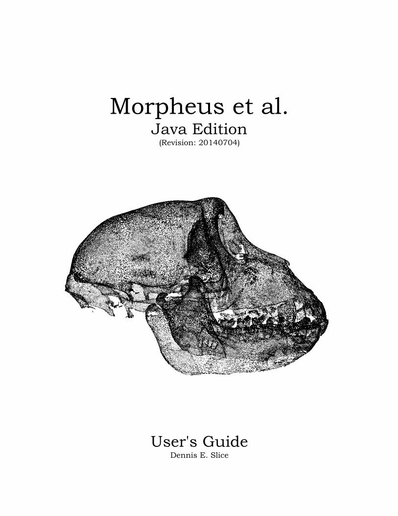
Cover Art: The image on the cover was generated by the author in Morpheus et al. It is the skull of a cynomolgus macaque (Macaca fascicularis) scanned by the FSU MorphLab's Breuckmann optoTop-HE structured light scanner. The surface was displayed as black vertices only on a white background. The original scan contains 887256 faces defined over 458797 vertices.
Morpheus et al.Java Edition
-Dennis E. Slice

[blank]
Table of Contents 1 Introduction..........................................................................................................1
1.1 Design Goals..................................................................................................1 1.1.1 Platform independence............................................................................2 1.1.2 Flexibility................................................................................................3 1.1.3 Extensibility............................................................................................4
1.2 Operational Model..........................................................................................5 1.3 First Look.......................................................................................................7 1.4 What's new?...................................................................................................8 1.5 References.....................................................................................................9
2 Installation and Execution..................................................................................11 2.1 Installation...................................................................................................11
2.1.1 Example Data Files...............................................................................13 2.1.2 Icons.....................................................................................................13
2.2 Execution.....................................................................................................13 2.3 Trouble Shooting..........................................................................................14
3 The Listing Pane.................................................................................................17 4 The Graphics Pane..............................................................................................19
4.1 Plot Options.................................................................................................27 4.1.1 General Plotting Options.......................................................................27 4.1.2 Group Plotting Options..........................................................................28
5 An Example........................................................................................................37 6 More Complex Examples.....................................................................................49
6.1 Whole-Configuration Reconstruction (with Batch Processing).......................49 6.2 High-dimensional Data................................................................................56 6.3 References....................................................................................................60
7 Commands.........................................................................................................63 7.1 File...............................................................................................................63
7.1.1 File|Open..............................................................................................64 7.1.2 File|Append..........................................................................................65 7.1.3 File|Save As..........................................................................................65 7.1.4 File|Close..............................................................................................66 7.1.5 File|Import............................................................................................66 7.1.6 File|Export............................................................................................67 7.1.7 File|New from images............................................................................67 7.1.8 File|New from images|2D.....................................................................68 7.1.9 File|New from images|3D.....................................................................68 7.1.10 File|Batch...........................................................................................69 7.1.11 File|Log...............................................................................................69 7.1.12 File|Log|Start.....................................................................................70 7.1.13 File|Log|Stop......................................................................................70 7.1.14 File|Exit..............................................................................................70
7.2 View.............................................................................................................70 7.2.1 View|Objects.........................................................................................71 7.2.2 View|Objects|Info.................................................................................71 7.2.3 View|Objects|Object i...........................................................................72
7.2.4 View|Objects|Groups...........................................................................73 7.2.5 View|Objects|List|Transformation parameters.....................................73 7.2.6 View|Points...........................................................................................74 7.2.7 View|Points|Report...............................................................................74 7.2.8 View|Points|Missing.............................................................................75 7.2.9 View|Points|Links................................................................................76 7.2.10 View|Points|Centroid Size..................................................................76 7.2.11 View|Points|Superimposition.............................................................77 7.2.12 View|Points|Superimposition|Options...............................................77 7.2.13 View|Points|Superimposition|SS.......................................................78 7.2.14 View|Points|Superimposition|SS|Mean.............................................78 7.2.15 View|Points|Superimposition|SS|Initial Reference............................78 7.2.16 View|Points|Superimposition|SS|Origin............................................78 7.2.17 View|User...........................................................................................78 7.2.18 View|User|UserVars...........................................................................79 7.2.19 View|User|Defines..............................................................................79 7.2.20 View|Measurements............................................................................80 7.2.21 View|Measurements|Definitions.........................................................80 7.2.22 View|Measurements|Values...............................................................80
7.3 Edit..............................................................................................................81 7.3.1 Edit|Objects..........................................................................................82 7.3.2 Edit|Objects|Group..............................................................................82 7.3.3 Edit|Objects|Group|By Count.............................................................83 7.3.4 Edit|Objects|Group|File......................................................................84 7.3.5 Edit|Objects|Group|Label....................................................................85 7.3.6 Edit|Objects|Group|Ungroup...............................................................85 7.3.7 Edit|Objects|Delete..............................................................................85 7.3.8 Edit|Objects|Keep................................................................................86 7.3.9 Edit|Objects|Reflect.............................................................................87 7.3.10 Edit|Objects|Rename.........................................................................87 7.3.11 Edit|Objects|Swap.............................................................................87 7.3.12 Edit|Objects|Add dimension...............................................................88 7.3.13 Edit|Objects|Merge with file...............................................................88 7.3.14 Edit|Points..........................................................................................89 7.3.15 Edit|Points|Adjust..............................................................................90 7.3.16 Edit|Points|Append............................................................................90 7.3.17 Edit|Points|Copy................................................................................91 7.3.18 Edit|Points|Delete..............................................................................91 7.3.19 Edit|Points|Demote............................................................................92 7.3.20 Edit|Points|Insert...............................................................................93 7.3.21 Edit|Points|Label...............................................................................93 7.3.22 Edit|Points|MakeMissing...................................................................94 7.3.23 Edit|Points|Promote...........................................................................94 7.3.24 Edit|Points|Swap...............................................................................95 7.3.25 Edit|Points|Compute..........................................................................96 7.3.26 Edit|Points|Compute|Distance-to-curve points..................................96 7.3.27 Edit|Points|Compute|Sample from curve...........................................97 7.3.28 Edit|Points|Sample from curve|Sample.............................................98
7.3.29 Edit|Points|Sample from curve|Merge...............................................99 7.3.30 Edit|Points|Links...............................................................................99 7.3.31 Edit|Points|Links|Add.......................................................................99 7.3.32 Edit|Points|Links|Remove...............................................................100 7.3.33 Edit|Points|Links|Clear...................................................................101 7.3.34 Edit|Points|Superimposition............................................................101 7.3.35 Edit|Points|Superimposition|Options..............................................101 7.3.36 Edit|Points|Superimposition|Options|Set.......................................102 7.3.37 Edit|Points|Superimposition|Options|Restore.................................103 7.3.38 Edit|User..........................................................................................103 7.3.39 Edit|User|UserVars..........................................................................104 7.3.40 Edit|User|UserVars|Edit..................................................................104 7.3.41 Edit|User|UserVars|Add..................................................................104 7.3.42 Edit|User|UserVars|Delete..............................................................104 7.3.43 Edit|User|Defines.............................................................................105 7.3.44 Edit|User|Defines|Set......................................................................105 7.3.45 Edit|User|Defines|Clear...................................................................105 7.3.46 Edit|User|Measurements.................................................................106 7.3.47 Edit|Measurements|Add...................................................................106 7.3.48 Edit|Measurements|Remove.............................................................107 7.3.49 Edit|Measurements|Clear................................................................107
7.4 Process.......................................................................................................108 7.4.1 Process|Points....................................................................................108 7.4.2 Process|Points|Superimposition.........................................................109 7.4.3 Process|Points|Superimposition|OPA................................................109 7.4.4 Process|Points|Superimposition|GPA................................................110 7.4.5 Process|Points|Superimposition|RF...................................................110 7.4.6 Process|Points|Superimposition|GRF................................................110 7.4.7 Process|Points|Superimposition|BSC................................................111 7.4.8 Process|Points|Superimposition|Restore............................................111 7.4.9 Process|Points|Superimposition|Restore|All......................................112 7.4.10 Process|Points|Superimposition|Restore|Scale................................112 7.4.11 Process|Points|Superimposition|Restore|Rotation...........................113 7.4.12 Process|Points|Superimposition|Restore|Translation......................113 7.4.13 Process|Points|Missing data.............................................................113 7.4.14 Process|Points|Missing data|Impute................................................114 7.4.15 Process|Points|Missing data|Impute|Simple mean substitution......114 7.4.16 Process|Points|Missing data|Impute|GPA mean substitution..........115
7.5 Analyze......................................................................................................118 7.6 Save...........................................................................................................118
7.6.1 Save|Objects.......................................................................................118 7.6.2 Save|Objects|Grand mean..................................................................118 7.6.3 Save|Objects|Group means................................................................119 7.6.4 Save|Objects|Transformation parameters...........................................119 7.6.5 Save|Points.........................................................................................119 7.6.6 Save|Points|Centroid Size..................................................................119 7.6.7 Save|Points|Analysis..........................................................................120 7.6.8 Save|User...........................................................................................121
7.6.9 Save|Measurements............................................................................121 7.7 System.......................................................................................................122
7.7.1 System|Stop graphics update.............................................................122 7.7.2 System|Desktop..................................................................................122 7.7.3 System|Deskptop|Size........................................................................123 7.7.4 System|Desktop|Defaults...................................................................123 7.7.5 System|Parameters.............................................................................123 7.7.6 System|Parameters|List.....................................................................124 7.7.7 System|Desktop|Parameters|Set.......................................................124 7.7.8 System|Listing font.............................................................................125 7.7.9 System|Desktop|Listing Font|Default................................................125 7.7.10 System|Desktop|Listing Font|Set....................................................125
7.8 Help...........................................................................................................125 7.8.1 Help|About.........................................................................................126
7.9 Unix-like Commands..................................................................................126 7.9.1 ls.........................................................................................................127 7.9.2 pwd.....................................................................................................127 7.9.3 cls.......................................................................................................127
8 The Configuration File......................................................................................129 9 Batch Processing..............................................................................................131
9.1 Batch-specific commands...........................................................................131 9.1.1 stop.....................................................................................................131 9.1.2 time.....................................................................................................131
10 Morpheus Data Files (.mdt).............................................................................133 11 Other Morpheus Formats................................................................................141
11.1 Morpheus grouping files (.grp)..................................................................141 12 Other Supported Data Formats.......................................................................143
12.1 Integrate (.lnd)..........................................................................................143 12.2 Morphologika (.txt)...................................................................................144 12.3 R (.Rdata).................................................................................................145 12.4 Raw (.raw)................................................................................................146 12.5 TPS (.tps)..................................................................................................146 12.6 NTSYSpc (.nts).........................................................................................148
13 Surface Formats.............................................................................................151 13.1 Wavefront (.obj)........................................................................................151 13.2 Polygon File Format (Stanford Triangle Format) (.ply)...............................152

ix
PrefaceI hope that my students learn some lessons from my own experience and mistakes. One of the more important of those is that few things are ever perfected or, even, finished. Instead, things often reach a level of usefulness that is sufficient to be shared. Such is the case with this latest version of Morpheus et al. I have worked on it for years, and I could easily work on it for many more and still not be satisfied that it was finished, much less perfected. Instead, I believe it is simply quite useful. So, I fixed the feature list in its current state and set about tying up the loose ends of documentation, distribution, etc. to create the package you have here. Of course, I will continue to work to expand and improve the program, and I now have a lab full of extremely competent student programmers and researchers who are, themselves, working diligently and enthusiastically to develop new functions and features that are expected to find their way into future versions of the program. For now, though, it is what it is. I hope you find it useful. -dslice
DISCLAIMERThe program, Morpheus et al.: Java Edition, and all documentation, files, scripts, etc. distributed with it are provided “As Is”. While I have attempted to check the accuracy of computations, data files, documentation, etc. and the safe performance of associated scripts, I accept no responsibility for the results of their use or misuse. No claims are made as to the suitability (or not) of the software and associated files for any particular purpose. By using this software, the user assumes all responsibility for subsequent results.

x
AcknowledgementsNo one person could claim sole credit for the development of a program such as Morpheus et al. As such, I am indebted to a vast number of individuals, many of whom remain nameless to me, as they were respondents to various online queries or sharers of clever routines for specific purposes.
Of those whose names I do know, of particular note are F. James Rohlf and Fred L. Bookstein. Jim Rohlf was my dissertation advisor and is still my general mentor who has always given freely of his vast knowledge on subjects such as, but not limited to, programming, statistics, and morphometrics. Fred Bookstein, with whom I have occasionally competed with for resources at the University of Vienna, is an icon in the field of morphometrics and has shown exceptional patience with me as I have tried to delve sufficiently deeply into the technical aspects of morphometrics and their underlying meaning.
Other individuals who cannot be overlooked are the late Leslie F. Marcus, who willingly and tirelessly, promoted my involvement in the morphometrics community and taught me how to enjoy international travel, and the late Marco Corti, who did so much for the promotion of advanced morphometric research.
I am also forever grateful for the support and encouragement given to me by Horst Seidler at the University of Vienna, who provided me a place and the means to teach and work on morphometric methods and software when I most needed them.
Of course, I cannot omit the contributions of so many colleagues, researchers, and students around the world, especially those in Vienna, whose problems and inquiries motivated me to find out more about morphometric methods and provide generally useful routines to address their own particular problems. Alas, this latter group is far too extensive to recognize individually.
This new release also affords me the opportunity to recognize the contributions of the inhabitants and local associates of the MorphLab at Florida State University. As of this writing, these include Thomas Campbell Arnold, Cameron Berkley, Kathryn O'D. Miyar, Benjamin Pomidor, James K. Soda, Detelina Stoyanova, Stephan Townsend, Olmo Zavala Romero, and Aki Watanabe. Specific, algorithmic contributions to the program are recognized individually within this document and the program, itself. Other collaborators who have inspired, through their own research questions, development of the program can be found on the MorphLab website at http://morphlab.sc.fsu.edu.
To all of these people, I am most appreciative and fully acknowledge their contribution to this effort, while taking sole responsibility for any mistakes

xi
herein.
This work was supported, in part and most recently, by Cooperative Research Agreement W911QY-12-2-0004 between Florida State University and the U.S. Army Natick Soldier Research, Development, and Engineering Center (http://www.army.mil/info/organization/natick/) and a contract from InfoSciTex Corp. This support in no way implies endorsement of the final product.

xii
1
1 IntroductionMorpheus et al. is a program designed to carry out generally useful functions related to geometric morphometrics (GM). If you have found, opened, and are reading this document, there is little reason to delve too deeply into what geometric morphometrics is other than, for completeness, to say that it is a field focused on the analysis of the shapes and forms of specimens of interest. What those shapes and forms are is generally unique to the individual researcher or project, but the methods employed to rigorously analyze them are shared across numerous and diverse disciplines.
1.1 Design GoalsEarly experience with morphometric software, e.g., GRF (Slice and Rohlf, 1989), revealed a number of problems with such domain-specific programs. Primarily, these program were, and still often are, written to perform fixed operations on perfect data conforming to the strict requirements of the software. Furthermore, these program were limited to a single computational platform. Those that did operate in multiple environments were often written in portable languages with only a rudimentary, command-line interface. GRF-ND (Slice, 1992) was an early attempt to address some of these shortcomings. It removed the restriction of morphometric analysis to two-dimensional data and allowed additional operational flexibility, but still was limited to a single computing environment and a rigid, limited data structure. With support from the U.S. National Science Foundation (BIR-9503024), it was undertaken to develop totally new, flexible software for morphometric analysis. This resulted in the first version of Morpheus et al. (Slice, 1996) and was somewhat successful. The new software supported varied, user-defined data types, tolerated incomplete data of any dimensionality, and was, initially, cross-platform, running in Windows, Unix, AIX, OS2 Warp, and Mac OS environments. However, the original Morpheus et al. was fatally flawed in that it depended upon commercial cross-platform libraries. The company responsible for those libraries never produced a promised graphical product for the MacIntosh and eventually, as might be expected, terminated support for their library in favor of dedicating their efforts to programming watches or some such nonsense. This eventually led to the program being effectively limited to the 16-bit Windows environments supporting only “8.3” DOS filenames. As such, the program never reached its full potential, though it still offers some functionality not readily found elsewhere.
Nevertheless, it was apparent that a new package needed to be developed. This was begun in 2005 with no external support. The design goals of that project, leading to the current Morpheus et al. program, were still to provide a platform-independent, flexible, and extensible environment for morphometric analysis.
2
How each of these goals was addressed is described in the following sections.
1.1.1 Platform independencePlatform independence, the ability of software to run in multiple computational environments, is a fundamental attribute I expect not only in the software I produce, but in all of the software I use on a regular basis. As I tell my student, I will not demand that they work in a particular environment or purchase a specific software package, and I do not expect them to impose such restrictions or make such demands on me. There really is no need, as there are ample high-quality, open-source, cross-platform programs available for most any need. The few exceptions for me include the very nice Osirix program (http://www.osirix-viewer.com/) that is written only for the Mac OS X environment (though I suspect alternatives for other systems are available) and certain document suites that I require to interact with colleagues who default to the use of proprietary software. For my own software development, platform independence is a basic requirement.
As was mentioned earlier, my initial attempts at achieving platform-independence was thwarted by my use of a commercial software library. Not wishing to repeat this expensive failure, I set about finding a non-commercial, well-supported platform with which to work. This led to Java (www.java.com).
The Java programming language is an interpreted language that runs on a virtual machine. That is, Java programs are compiled into Java-specific byte-code that is then executed on a “virtual machine” that is written for a particular operating environment. Reasonably carefully crafted programs are, then, platform independent and can run on any system for which a virtual machine is available. Currently, virtual machines are available for MS Windows, Mac OS X, and various flavors of Linux/Unix operating systems. In addition, Java is also supported in high-performance computing environments, which are often based, themselves, on Linux.
One critical issue in deciding to develop the new Morpheus using the Java language was acceptance and potential longevity. Java is a mature, widely accepted language that regularly competes, and usually exceeds, the “C” language for the top spot in programming popularity (e.g., http://www.tiobe.com/index.php/content/paperinfo/tpci/index.html). Furthermore, Java programmers are frequently some of the most sought-after people in the IT industry. This last observation gives me assurance that by encouraging my students to learn and use Java, I am not only addressing my own needs and those of the morphometrics community, but providing them with valuable experience for their own career development.
Along with the underlying platform independence of the Java language, it also provides a sophisticated graphical user-interface environment through its
3
Swing libraries, as well as several others should one chose to avail themselves of them. Furthermore, the Java community also supports sophisticated libraries for access to accelerated, three-dimensional graphics provided by the OpenGL language. Platform- and hardware-specific libraries for accessing these features are available for most platforms, and access to them from within Java is possible through the Jogl interface (https://jogamp.org/jogl/www/) supported by an active and talented group of developers.
Still, though the Java language provides a sophisticated graphical environment and access to high-performance, hardware-specific graphics engines, the underlying design of the latest version of Morpheus et al. keeps these features segregated from the computational components of the program necessary for morphometric analysis. In this way, a version of the program could be developed (such is planned for the near future 1) that would be completely independent of any graphical environment or hardware.
1.1.2 FlexibilityA common problem with task-specific software is its limitation to specific analyses determined by the programmer of particular types of data adhering to inflexible formatting requirements. Such an environment often restricts the user's scope of analysis and, in general, research creativity. One fundamental principal that informed both the computational model of Morpheus et al. and its data-file format was to eliminate, to the extent possible, this type of constraint.
This makes for a significant programming challenge, as routines must be developed to process data about which little may be known in advance. In morphometric research, this generally includes sample size, of course, but also data dimensionality. Researchers may also want to include with their data non-morphometric information that is not part of the fundamental morphometric operations they seek to perform within a program and may want to quantify aspects of their data that are not strictly part of the GM paradigm.
To address these issues, Morpheus et al. takes advantage of the object-oriented programming model by using dynamic, “self-aware” data structures. For instance, points2 are stored in linked lists of point-class objects (in the 1 Speculation about future features of the program has been intentionally limited in this
documentation. One can always say one is intending to do all sorts of useful and amazing things, but until they are actually available, they are of no use to the end user and their anticipation can result in lost time and research opportunities. In the case of a purely command-line version of Morpheus, this is a fairly trivial proposition and is high on the TODO list for development. I expect it to be available in the next release. ← I was wrong. Maybe next time.
2 Because of the generalized nature of the design of the software, we refer to “points” and “curves” instead of “landmarks” and “outlines”. Your points and curves may, in fact, be proper landmarks and outlines, but that is not required by the program.
4
programming sense), each of which maintains its own labeling and dimensionality information along with the coordinates of the points. Similarly, the specimens or objects in a data set are object-class objects that keep track of the types of data available, their location, and other ancillary information. These, in turn, are maintained by object-list-class objects that maintain and provide access to object-level operations. All computations within the program query the list, object, or specific data element for the information necessary to carry out the required operation. With this architecture, relatively few restrictions are placed on the data to be processed by the program.
The file format, itself, helps further this goal. Described in more detail in the “Morpheus data files (.mdt)” chapter of this document, the format of Morpheus data files provides support for a number of data types not necessarily specific to morphometric analysis and the flexible specification of those that are. For instance, the dimensionality of points and curves is specified within the data file, and user-defined variables in string, character, integer, and decimal format are supported. There are no prerequisites as to the number or, even, order of such elements in a data file. Nor is it required that all objects in a data file have the same number of components of a particular type. Specific computations, however, may require a common number and order of a particular type of data, but this is checked only when the computation is to be performed. In this way, researchers can include with their morphometric data almost any other information they would like to keep associated with their specimens. This information, while possibly not used at all by the program, remains intact and can be utilized in other analyses within other analytical environments.
The goal of flexibility extends to the organization of the computational components, as well. Operations, such as the computation of the grand mean, are carried out independently of any other operations. One does not have to, for instance, perform a generalized Procrustes analysis (GPA) to compute the grand mean of the current point data, though computation of the mean is part of the GPA operation. This means that one can load point-coordinate data whether or not it is appropriate for superimposition and compute and save the mean. For instance, one might have coordinates that represent standard types of measurements, e.g., lengths, widths, heights, and use Morpheus to compute the mean values for these variables.
1.1.3 ExtensibilityThe desire for extensibility is incorporated into all aspects of the program from its overall organization, to its computational components, to its file structure. To the extent possible, and this is a fairly great extent due to the object-oriented nature of the program, software components operate independently of one another. One component may be aware of another, but it need not know anything of the details of its organization. Instead, the second component
5
provides an interface that allows the first to query it as to any required information. The superimposition routines, for instance, ask the object list how many objects are available and their dimensionality, it then proceeds with the superimposition process by checking the objects in the list for consistency in the number and organization of their primary points3 and carrying out the superimposition based on this information.
By sequestering data-specific information to within a data class to the extent possible and providing the means to query the data structure, new routines can be easily developed that require only knowledge of how to ask the data structures about their contents. The program then needs only to be told about the existence of such a routine via the command-line processor and, usually, the addition of menu items for that routine.
The file format is similarly designed for extensibility. Basic organization is not rigidly structured with a few, generally optional, directives being required at the beginning of the file followed by fairly unstructured sets of points, variables, curves, etc. packaged into data objects. Such a design allows for the easy addition of new, useful data types as they are identified.
1.2 Operational ModelIt is worth a few words on the operational model of Morpheus to give the user an idea of what is going on “behind the scenes” when the program is run. Basically, when a data file is read in, an initially empty list is created to hold the data. This list maintains and provides access to certain global information about the data, such as the source filename, the dimensionality of the data, user-defined measurements to be made across all objects, and graphical links to facilitate visualization of an individual object. Next, data for individual objects are read in. These objects are added to the list, which maintains them as a linked list. The objects, themselves, are initially empty except for label information. As data for an object is read from a file, they are added to the list according to their type, e.g., points, curves, images, etc. The object maintains its own, separate lists of these data.
When part of the program is ready to carry out computations on the data, it usually does so through the main object list. From this list, it can determine the number of objects contained therein, their dimensionality, and globally defined measurements. If the routine needs to operate on individual objects, it
3 Points (and some other data types) are classified as either “primary” or “secondary” allowing the subsetting of data within a data type for a particular analysis. For example, a point/landmark-based superimposition will estimate the transformation parameters using only the primary points, but apply that transformation to all coordinate-based data, such as secondary points. Point state is specified in the data file and can be set by the user through the “demote” and “promote” commands within the program. See the “Commands” chapter for details.

6
asks the list for pointers to specific objects. These can be used to query the object, itself, about the numbers and types of data it contains, and, when needed, the object can be asked to provide specific data.
Overall, the organization looks something like this for point/landmark data:
Object List (label, file, dimensionality, measurements, links, number of objects)
– Object i (label, dimensionality, point lists, curve lists, etc.)
– Point List (dimensionality, number of points, etc.)
– Point (label, dimensionality, coordinate array)
Under this organization, existing routines can function without the need for hard-coded knowledge of the available data, and new data types and structures can be added without interfering with existing structures or the routines that use them.
7
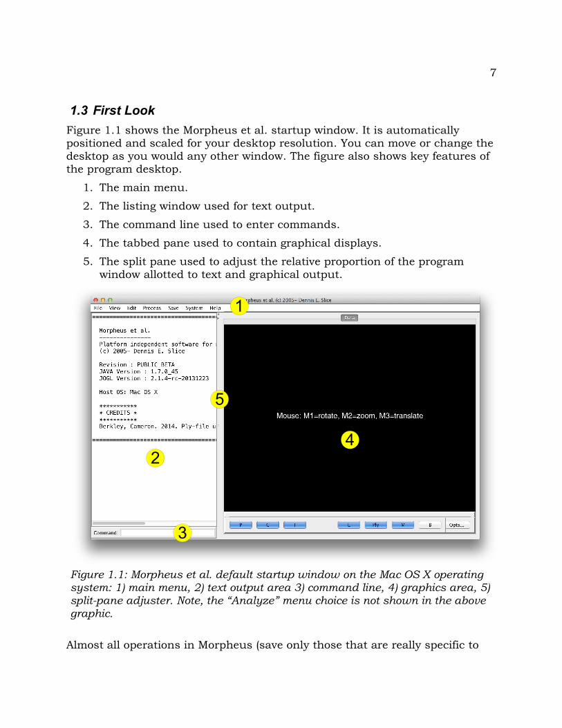
1.3 First LookFigure 1.1 shows the Morpheus et al. startup window. It is automatically positioned and scaled for your desktop resolution. You can move or change the desktop as you would any other window. The figure also shows key features of the program desktop.
1. The main menu.
2. The listing window used for text output.
3. The command line used to enter commands.
4. The tabbed pane used to contain graphical displays.
5. The split pane used to adjust the relative proportion of the program window allotted to text and graphical output.
Almost all operations in Morpheus (save only those that are really specific to
Figure 1.1: Morpheus et al. default startup window on the Mac OS X operating system: 1) main menu, 2) text output area 3) command line, 4) graphics area, 5) split-pane adjuster. Note, the “Analyze” menu choice is not shown in the above graphic.
1
2
5
4
3

8
the graphical interface) are controlled by commands. These commands can be entered by the user at the command line (no. 3 above) or read from a batch file for parsing and processing. The menu system (no. 1 above), again except for things like the desktop size that are specific to the graphical interface, serves simply to gather data to generate command lines that are then submitted for processing. The commands are printed in the listing window (no. 2 above) prior to processing so that you can use the commands to get the proper syntax to use in batch files.
The default graphics window is displayed in a sub-window on the right (4 in Figure 1.1). With no data loaded, floating interaction hints are display. As you might surmise, pressing and holding the first (left) mouse button allows the user to grab and rotate the scene, the second (middle) mouse button zooms the image, and the third (right) mouse button moves the scene up and down or left and right. The divider between the listing and graphics windows can be adjusted to show more or less of one or the other, and the current division is saved when the program is terminated with the “File|Exit” command. This proportion is restored the next time the program is run. Additional graphical output is added to this area, and specific plots can be selected via tabs that appear at the top of the pane.
1.4 What's new?Those familiar with earlier version of the Java edition of Morpheus et al will recognize that the program has undergone extensive organizational changes. The most apparent of these is that the graphics window, which was previous a separate, free-floating window, has been incorporated into the main program window. The main program window is now divided into two panes. The leftmost is used for the command line and text output, and the right is used for graphical output. These are, in fact, two components of a “split pane” and the amount of area allocated to each sub-pane can be adjusted by the bar in between. This can be manually adjusted or arrows on the bar can be used to have the text area or the graphical area fill the program window (aside from the menu area, of course). When the user exits the program via the “File|Exit” command, the proportion allocated to text and graphics is saved and restored when the program is restarted. Furthermore, the graphical area is actually a tabbed pane, and additional graphical output can be added to it. Specific graphical displays are then selected by the tabs at the top of this area.
The menus, too, have been extensively reorganized. The main menu now contains selections for “File”, “View”, “Edit”, “Process”, “Analyze”, “Save”, “System”, and “Help” selections. The first of these represent a normal flow of program interaction. The user opens a data file (“File”), views various properties of the loaded data (“View”), may edit the data by adding or modifying points (“Edit”), may further process the data by Procrustes superimposition or other
9
computational methods (“Process”), analyze the current data (“Analyze”), and save various results (“Save”). The “System” and “Help” items provide additional program-wide information or functions. The choices, many of which are new, available under these main headings are discussed in detail later in this document.
Another major addition to this version is the use of an “iSeq” parameter for specifying sequences of item indices. Previous versions of the program required the user to specify items to be operated upon one at a time. That is, commands to be applied to multiple items had to be entered for each item. With the iSeq, sets of items can be specified. What items are indexed is specific to the operation being performed. The general syntax of an iSeq is a series of index specifications separated by commas. No spaces are allowed, and ranges are supported by use of the '-' character. If a range begins with a '-', then indexing from the first item in the list is assumed. If it ends with a '-', then indexing is assumed to extend to the last item. Unique (redundancies are eliminated) items are sorted as appropriate for the command being used.
For instance, assuming a set of seventy-three items., a relevant iSeq might look like:
-3,8,12,16-19,8,17,71-
Such an iSeq would be parsed as:1,2,3,8,12,16,17,18,19,8,17,71,72,73
Then sorted:1,2,3,8,8,12,16,17,17,18,19,71,72,73
And cleaned up to produce:1,2,3,8,12,16,17,18,19,71,72,73
For some multiple operations, item indexing might lead to certain ambiguities. For instance, if one wanted to delete items 4 and 7 from a list, if one deletes item 4 first, does one then delete the current item 7 (all indices have been reduced by one) or the item 7 in the original list. To address this, it is assumed that all indices in a particular iSeq refer to the original position. So, for some operations, e.g., insertions and deletions, the operations are performed using the iSeq indices in descending index order. When such ambiguities are not present, operations are performed from lowest to highest index.
1.5 ReferencesSlice, D. E. 1992. GRF-ND: N-dimensional Rotational Fitting and Analysis. Stony Brook, NY, USA: Department of Ecology and Evolution, SUNY, Stony Brook.

10
Slice, D. E. 1996. Morpheus et al.: Cross-platform Software for Morphometric Research. Stony Brook, NY, USA: Department of Ecology and Evolution, SUNY, Stony Brook.
Slice, D. E., and F. J. Rohlf. 1989. GRF: Generalized Rotational Fitting Program. Stony Brook, NY, USA: Department of Ecology and Evolution, SUNY, Stony Brook.
11
2 Installation and Execution
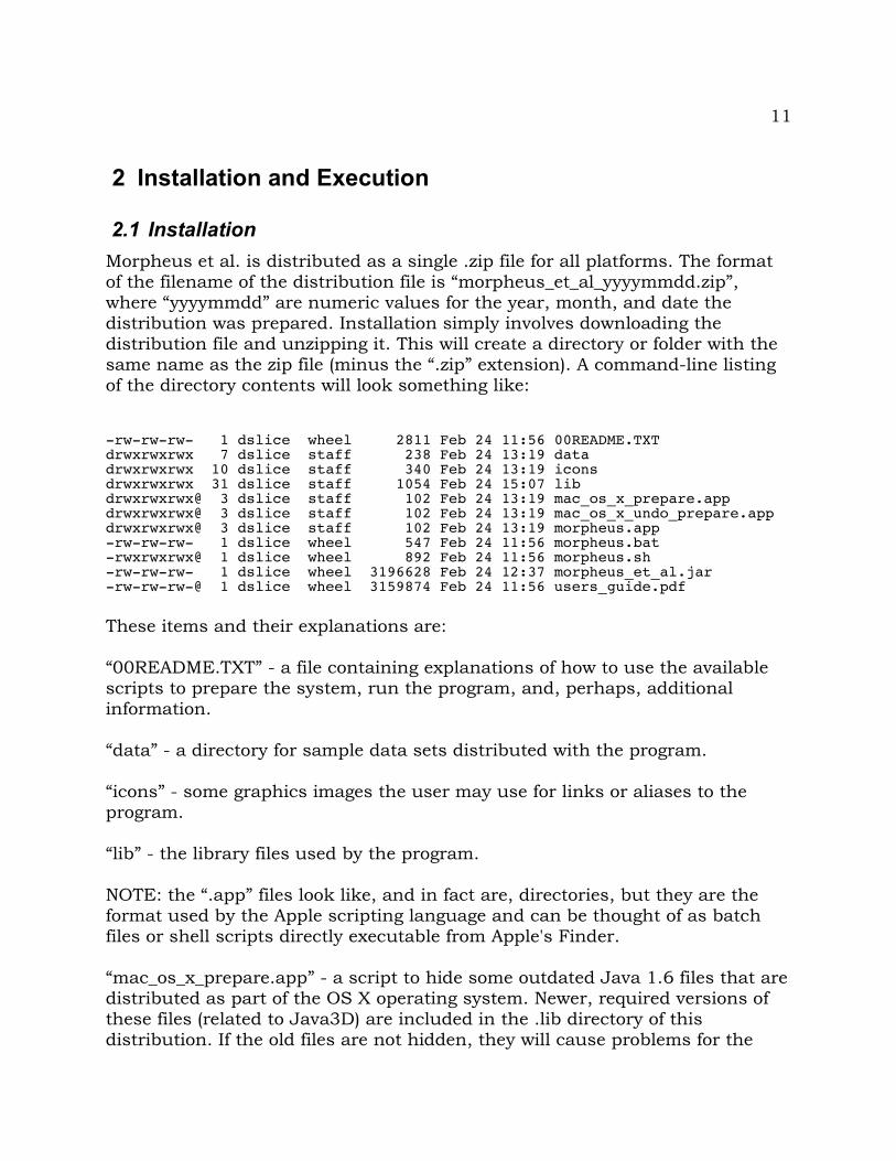
2.1 InstallationMorpheus et al. is distributed as a single .zip file for all platforms. The format of the filename of the distribution file is “morpheus_et_al_yyyymmdd.zip”, where “yyyymmdd” are numeric values for the year, month, and date the distribution was prepared. Installation simply involves downloading the distribution file and unzipping it. This will create a directory or folder with the same name as the zip file (minus the “.zip” extension). A command-line listing of the directory contents will look something like:
-rw-rw-rw- 1 dslice wheel 2811 Feb 24 11:56 00README.TXTdrwxrwxrwx 7 dslice staff 238 Feb 24 13:19 datadrwxrwxrwx 10 dslice staff 340 Feb 24 13:19 iconsdrwxrwxrwx 31 dslice staff 1054 Feb 24 15:07 libdrwxrwxrwx@ 3 dslice staff 102 Feb 24 13:19 mac_os_x_prepare.appdrwxrwxrwx@ 3 dslice staff 102 Feb 24 13:19 mac_os_x_undo_prepare.appdrwxrwxrwx@ 3 dslice staff 102 Feb 24 13:19 morpheus.app-rw-rw-rw- 1 dslice wheel 547 Feb 24 11:56 morpheus.bat-rwxrwxrwx@ 1 dslice wheel 892 Feb 24 11:56 morpheus.sh-rw-rw-rw- 1 dslice wheel 3196628 Feb 24 12:37 morpheus_et_al.jar-rw-rw-rw-@ 1 dslice wheel 3159874 Feb 24 11:56 users_guide.pdf
These items and their explanations are:
“00README.TXT” - a file containing explanations of how to use the available scripts to prepare the system, run the program, and, perhaps, additional information.
“data” - a directory for sample data sets distributed with the program.
“icons” - some graphics images the user may use for links or aliases to the program.
“lib” - the library files used by the program.
NOTE: the “.app” files look like, and in fact are, directories, but they are the format used by the Apple scripting language and can be thought of as batch files or shell scripts directly executable from Apple's Finder.
“mac_os_x_prepare.app” - a script to hide some outdated Java 1.6 files that are distributed as part of the OS X operating system. Newer, required versions of these files (related to Java3D) are included in the .lib directory of this distribution. If the old files are not hidden, they will cause problems for the

12
program. These files are in the /System/Library/Java/Extensions directory. The script moves them to a subdirectory there called “hold_j3d”. Because this is a system directory, the user will be asked several times for an administrative password to carry out the necessary operations. These files may still be present even if you have installed a more recent Java 1.7 version. So, one still might have to run this script or figure out how to delete 1.6 from your system. We leave that as an exercise and test of your internet search skills.
“mac_os_x_undo_prepare.app” - a script to undo the actions of the above script. This is not likely to be necessary for most users, but is provided for completeness.
N.B. Execution of the “prepare” script is not necessary if you (or the OS) has not installed Apple's Java 1.6 on your system.
“morpheus.app” - a script to execute the program under OS X. While the program may be executed directly by double-clicking the morpheus_et_al.jar file, this does not allocate additional memory the program may need, and the program may not be executed from the correct subdirectory. This script does both. What it actually does is invoke the shell script “morpheus.sh” that is provided for linux systems and can be used under OS X from the command line. This script may be edited with an ASCII text editor to change the amount of memory allocated to the program.
“morpheus.bat” - a batch file to execute the program under MS Windows. While the program may be executed directly by double-clicking the morpheus_et_al.jar file, this does not allocated additional memory the program may need, and the program may not be executed from the correct subdirectory. This batch file does both, and may be edited with an ASCII text editor to change the amount of memory allocated to the program.
“morpheus.sh” - a shell script to execute the program under unix-like operating systems. While the program may be executed directly by double-clicking the morpheus_et_al.jar file, this does not allocated additional memory the program may need, and the program may not be executed from the correct subdirectory. This script does both. It can be used under the linux operating system or from the command line in OS X, and it may be edited with an ASCII text editor to change the amount of memory allocated to the program.
“morpheus_et_al.jar” - the actual Morpheus et al. program. While the program may be executed directly by double-clicking this file, this does not allocated additional memory the program may need and may not execute from the correct subdirectory. One should use one of the provided platform-specific

13
execution scripts.
“users_guide.pdf” - the Morpheus et al. user's guide (this file).
2.1.1 Example Data FilesA number of example data files are provided with the program in the “data” subdirectory. The contents of this subdirectory are:
-rw-rw-rw- 1 dslice wheel 1056 Feb 24 11:56 00README.TXTdrwxrwxrwx 12 dslice staff 408 Feb 24 13:19 2ddrwxrwxrwx 7 dslice staff 238 Feb 24 13:19 3ddrwxrwxrwx 7 dslice staff 238 Feb 24 13:19 batchdrwxrwxrwx 3 dslice staff 102 Feb 24 13:19 nd
“00README.TXT” - a text file describing the subdirectory contents.
“2d” - various data sets of two-dimensional data.
“3d” - data sets of three-dimensional data.
“batch” - files and data illustrating the use of Morpheus's batch-file processing system.
“nd” - sample data files of n-dimensional data.
2.1.2 IconsThe “icons” directory provides a number of graphics files (e.g., the morpheus macaque) in various formats the user may wish to associate with the program or its executing scripts. The .xcf extension is a Gimp-format file (http://www.gimp.org/) that can be modified in that program. The “.png” files are in portable network graphics format, and the other files are OS X Finder icons. The free, online icon convertor at http://iconverticons.com/ is a useful resource for creating your own icons. For OS X, for instance, upload the graphics file to the website, convert the file, and save the “.hqx” version. Double-clicking on the downloaded file will unpack the icon that can be directly dropped onto a file's “Get info” dialog icon.
2.2 ExecutionMorpheus et al. may be run from most operating systems by double-clicking the morpheus_et_al.jar file. However, this may not provide sufficient memory to the program for larger data sets, and the program may not be executed from the appropriate subdirectory. Hence, a number of platform-specific scripts are
14
provided for this purpose. These are “morpheus” (as it appears in Finder) for OS X, “morpheus.bat” for MS Windows, and “morpheus.sh” for unix-like operating systems (Linux and the Mac OS X command-line). It is preferable to run the program by executing these scripts.
Furthermore, DO NOT move these scripts from the directory. They need to be in their original locations in the main distribution directory to find the necessary files and libraries. For more convenient remote execution, create an alias or link to the appropriate execution script and move that link to the desired location, e.g., the operating system desktop.
The Morpheus et al. distribution directory, on the other hand, can be moved to any convenient location.
2.3 Trouble ShootingSimply unzipping the distribution file and clicking on the program launcher for your platform (see below) should run the program. However, it is practically impossible for us to check the program under all possible combinations operating system and hardware/software revisions. If it does not run after unzipping and clicking, one might need to seek help from someone proficient in your operating system and/or Java installation and configuration. The program has been developed at various times under Linux, Windows, and, for the most part, Mac OS X, and it is known to run without incident under all such operating systems. Some environments have reported problems, however. For instance, at a recent workshop, all participants running a version of Windows (no one seems to have had the same version) were able to run the program straight out of the archive. A few Mac users had problems.
There are a couple of known complexities in the Mac OS X environment. The first of these relates to Apple's original development and maintenance of its own Java 1.6 engine. Apple did not do a very good job of updating the engine, and, unfortunately, included (and still includes) additional libraries that conflict with more modern ones used by Morpheus. That is the purpose of the mac_os_x_prepare.app and mac_os_x_undo_prepare.app described below. Basically, these just move out-of-date files out the way so Morpheus doesn't try to use them, or put them back if you wish.
Java, however, is into version 1.7 (early versions of 1.8 are available as of this writing), so that is the best choice if you don't have Apple's 1.6 installed. Even if you have installed 1.7 (or later), the 1.6 files will still interfere with program operation if they are lying about.
A second subtlety with Java 1.7 on the Mac is that it is geared more toward running online apps than standalone ones like Morpheus et al. As a result, installing the 1.7 JRE (Java Runtime Environment) doesn't set up the system

15
for running standalone apps on Mac OS X (since all of our platforms are set up for development, we do not know if this is the case for other OSs.). One should instead install the JDE (Java Development Environment - http://www.oracle.com/technetwork/java/javase/downloads/jdk7-downloads-1880260.html). That should work.
Still some Mac users mentioned above were still unable to get the program running properly. In one case, the system was running OS 10.9 and would run the program from the command line, but the .app scripts would not execute. In two others, nothing would work – scripts or app. Both of these systems were running OS 10.7 and, initially, Java 1.6. Upgrading to Java 1.7 JDK did not help.
If you have a problem, please let us know and, best of all, try to seek local expertise in resolving the issue. As problems are identified and solved, these solutions will be announced and included in this documentation.

16
17
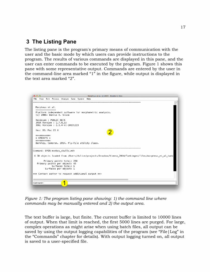
3 The Listing PaneThe listing pane is the program's primary means of communication with the user and the basic mode by which users can provide instructions to the program. The results of various commands are displayed in this pane, and the user can enter commands to be executed by the program. Figure 1 shows this pane with some representative output. Commands are entered by the user in the command-line area marked “1” in the figure, while output is displayed in the text area marked “2”.
Figure 1: The program listing pane showing: 1) the command line where commands may be manually entered and 2) the output area.
The text buffer is large, but finite. The current buffer is limited to 10000 lines of output. When that limit is reached, the first 5000 lines are purged. For large, complex operations as might arise when using batch files, all output can be saved by using the output logging capabilities of the program (see “File|Log” in the “Commands” chapter for details). With output logging turned on, all output is saved to a user-specified file.
1
2

18
Commands and output can be copied from the listing pane, and copied commands can be pasted into the command line for editing and/or re-execution. In most cases, the menu system is used to generate appropriately formatted commands, but with some familiarity with the program, the user may tend to enter simpler commands directly through the command line. This may require clicking the command area with the mouse to give it “focus” for accepting input.
19
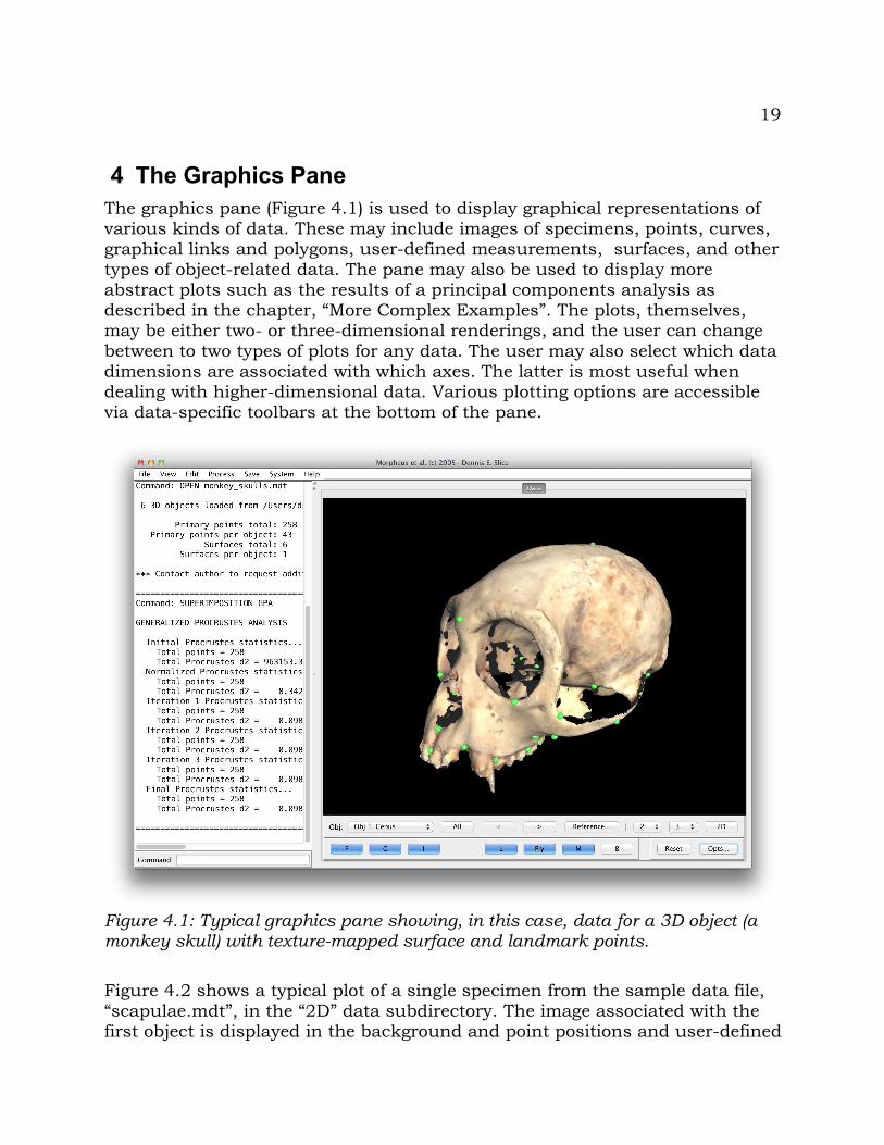
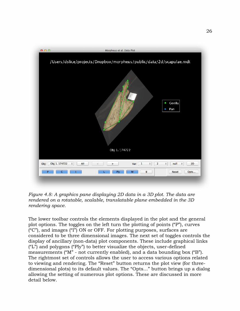
4 The Graphics PaneThe graphics pane (Figure 4.1) is used to display graphical representations of various kinds of data. These may include images of specimens, points, curves, graphical links and polygons, user-defined measurements, surfaces, and other types of object-related data. The pane may also be used to display more abstract plots such as the results of a principal components analysis as described in the chapter, “More Complex Examples”. The plots, themselves, may be either two- or three-dimensional renderings, and the user can change between to two types of plots for any data. The user may also select which data dimensions are associated with which axes. The latter is most useful when dealing with higher-dimensional data. Various plotting options are accessible via data-specific toolbars at the bottom of the pane.
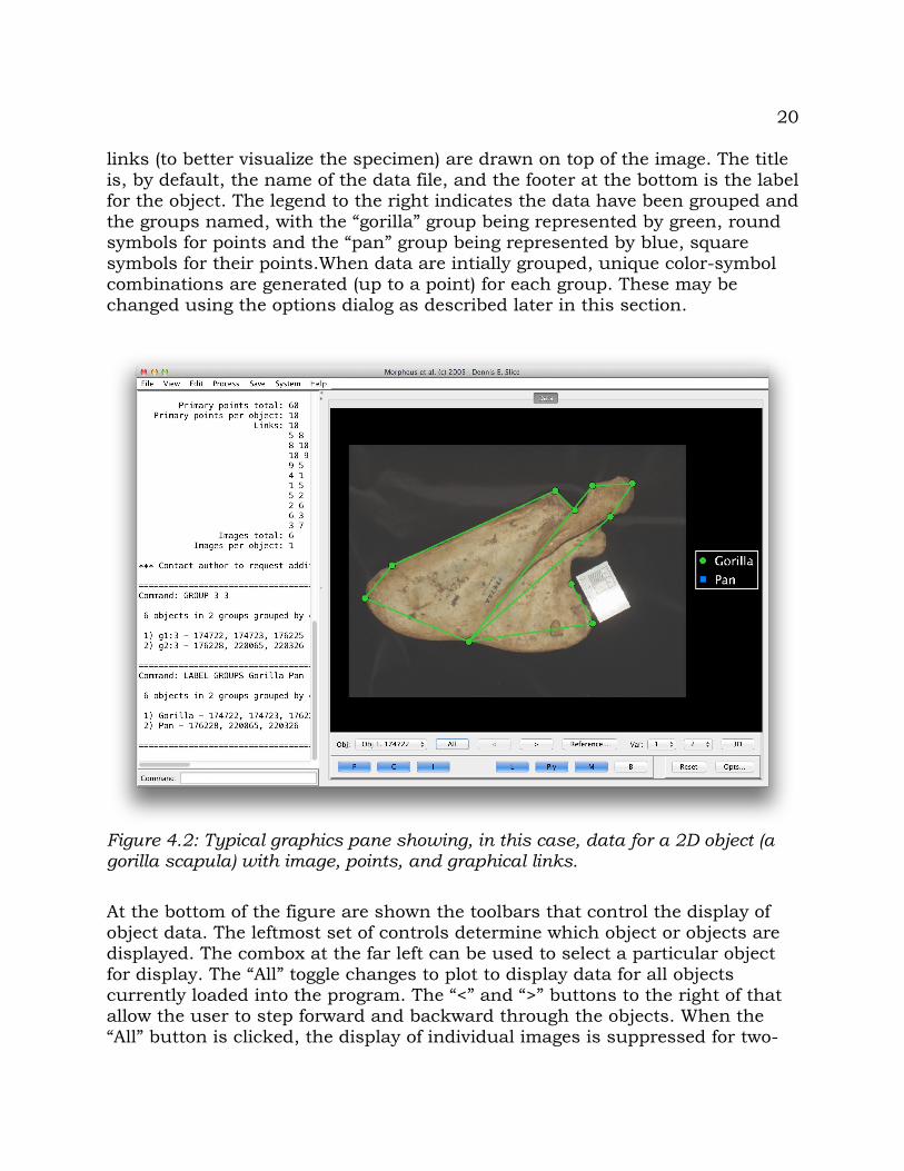
Figure 4.2 shows a typical plot of a single specimen from the sample data file, “scapulae.mdt”, in the “2D” data subdirectory. The image associated with the first object is displayed in the background and point positions and user-defined
Figure 4.1: Typical graphics pane showing, in this case, data for a 3D object (a monkey skull) with texture-mapped surface and landmark points.
20
links (to better visualize the specimen) are drawn on top of the image. The title is, by default, the name of the data file, and the footer at the bottom is the label for the object. The legend to the right indicates the data have been grouped and the groups named, with the “gorilla” group being represented by green, round symbols for points and the “pan” group being represented by blue, square symbols for their points.When data are intially grouped, unique color-symbol combinations are generated (up to a point) for each group. These may be changed using the options dialog as described later in this section.
At the bottom of the figure are shown the toolbars that control the display of object data. The leftmost set of controls determine which object or objects are displayed. The combox at the far left can be used to select a particular object for display. The “All” toggle changes to plot to display data for all objects currently loaded into the program. The “<” and “>” buttons to the right of that allow the user to step forward and backward through the objects. When the “All” button is clicked, the display of individual images is suppressed for two-
Figure 4.2: Typical graphics pane showing, in this case, data for a 2D object (a gorilla scapula) with image, points, and graphical links.
21
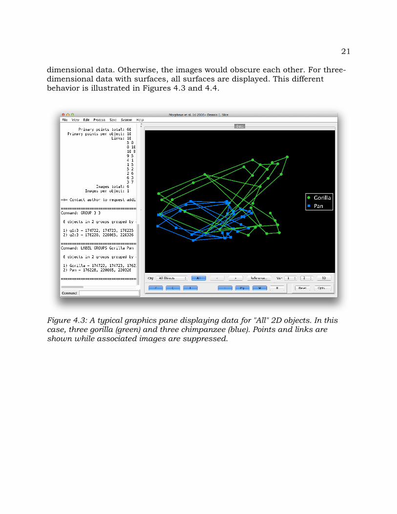
dimensional data. Otherwise, the images would obscure each other. For three-dimensional data with surfaces, all surfaces are displayed. This different behavior is illustrated in Figures 4.3 and 4.4.
Figure 4.3: A typical graphics pane displaying data for "All" 2D objects. In this case, three gorilla (green) and three chimpanzee (blue). Points and links are shown while associated images are suppressed.
22
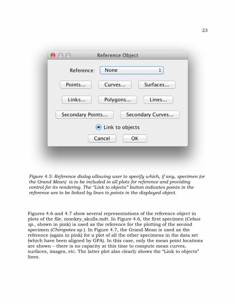
The “Reference” button presents a dialog (Figure 4.5) that allows the user to specify a specimen to include in all plots for reference purposes. The drop-down menu at the top allows the specification of the grand mean or one of the data objects to be used as the reference. At this time, only the points (not surfaces or curves) of the grand mean are displayed. Other buttons invoke dialogs that allow the specification of how elements of the reference object are to be rendered. These are the same dialogs used for object rendering and are explained in detail below. The “Link to objects” toggle enables the drawing of lines from the reference points to their homologs on individual data objects. This allows for an assessment of consistent point ordering, especially when point clouds overlap – lines will extend from the reference into another point cloud if points are out of order.
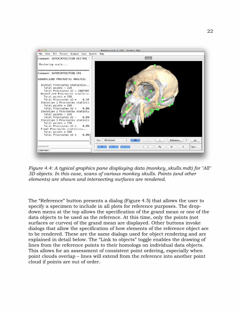
Figure 4.4: A typical graphics pane displaying data (monkey_skulls.mdt) for "All" 3D objects. In this case, scans of various monkey skulls. Points (and other elements) are shown and intersecting surfaces are rendered.
23
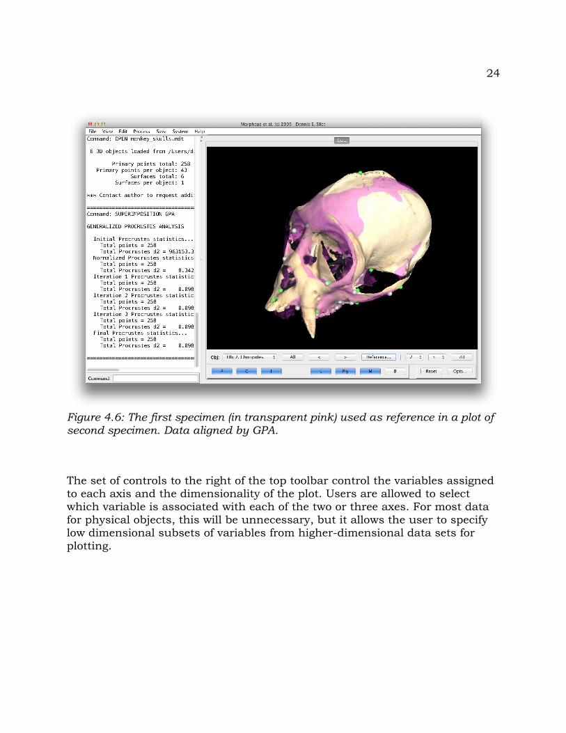
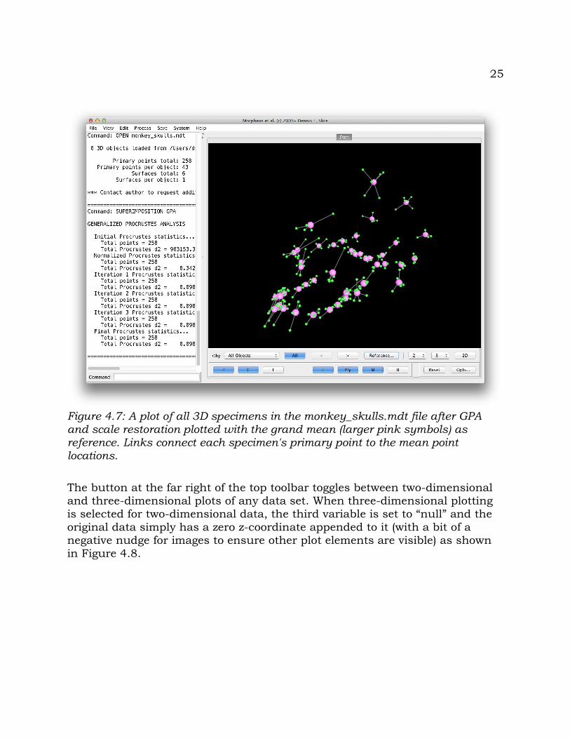
Figures 4.6 and 4.7 show several representations of the reference object in plots of the file, monkey_skulls.mdt. In Figure 4.6, the first specimen (Cebus sp., shown in pink) is used as the reference for the plotting of the second specimen (Chiropotes sp.). In Figure 4.7, the Grand Mean is used as the reference (again in pink) for a plot of all the other specimens in the data set (which have been aligned by GPA). In this case, only the mean point locations are shown – there is no capacity at this time to compute mean curves, surfaces, images, etc. The latter plot also clearly shows the “Link to objects” lines.
Figure 4.5: Reference dialog allowing user to specify which, if any, specimen (or the Grand Mean) is to be included in all plots for reference and providing control for its rendering. The “Link to objects” button indicates points in the reference are to be linked by lines to points in the displayed object.
24
The set of controls to the right of the top toolbar control the variables assigned to each axis and the dimensionality of the plot. Users are allowed to select which variable is associated with each of the two or three axes. For most data for physical objects, this will be unnecessary, but it allows the user to specify low dimensional subsets of variables from higher-dimensional data sets for plotting.
Figure 4.6: The first specimen (in transparent pink) used as reference in a plot of second specimen. Data aligned by GPA.
25
The button at the far right of the top toolbar toggles between two-dimensional and three-dimensional plots of any data set. When three-dimensional plotting is selected for two-dimensional data, the third variable is set to “null” and the original data simply has a zero z-coordinate appended to it (with a bit of a negative nudge for images to ensure other plot elements are visible) as shown in Figure 4.8.
Figure 4.7: A plot of all 3D specimens in the monkey_skulls.mdt file after GPA and scale restoration plotted with the grand mean (larger pink symbols) as reference. Links connect each specimen's primary point to the mean point locations.
26
The lower toolbar controls the elements displayed in the plot and the general plot options. The toggles on the left turn the plotting of points (“P”), curves (“C”), and images (“I”) ON or OFF. For plotting purposes, surfaces are considered to be three dimensional images. The next set of toggles controls the display of ancillary (non-data) plot components. These include graphical links (“L”) and polygons (“Ply”) to better visualize the objects, user-defined measurements (“M” - not currently enabled), and a data bounding box (“B”). The rightmost set of controls allows the user to access various options related to viewing and rendering. The “Reset” button returns the plot view (for three-dimensional plots) to its default values. The “Opts...” button brings up a dialog allowing the setting of numerous plot options. These are discussed in more detail below.
Figure 4.8: A graphics pane displaying 2D data in a 3D plot. The data are rendered on a rotatable, scalable, translatable plane embedded in the 3D rendering space.
27
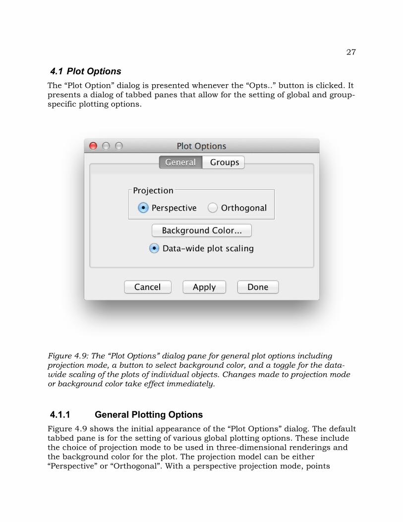
4.1 Plot OptionsThe “Plot Option” dialog is presented whenever the “Opts..” button is clicked. It presents a dialog of tabbed panes that allow for the setting of global and group-specific plotting options.
4.1.1 General Plotting OptionsFigure 4.9 shows the initial appearance of the “Plot Options” dialog. The default tabbed pane is for the setting of various global plotting options. These include the choice of projection mode to be used in three-dimensional renderings and the background color for the plot. The projection model can be either “Perspective” or “Orthogonal”. With a perspective projection mode, points
Figure 4.9: The “Plot Options” dialog pane for general plot options including projection mode, a button to select background color, and a toggle for the data-wide scaling of the plots of individual objects. Changes made to projection mode or background color take effect immediately.
28
equidistance apart appear closer together when farther away than when they are closer to the viewer. This simulates actual human vision, where parallel lines (e.g., the rails of a train track) appear to converge in the distance. With an orthogonal projection model, relative distances between points are preserved regardless of their distance from the viewer. The latter is probably a more reasonable projection for scientific usage, but this (in the current graphics system) precludes the ability to zoom in on parts of the plot. Therefore, the program uses the perspective projection by default.
Clicking the “Background Color...” button brings up a color dialog that provides the user with a variety of ways to select the background color for the plot.
The “Data-wide plot scaling” toggle, if selected, specifies that plots of individual objects are to be based on the range of values found across the entire data set. That is scaling (and offset) factors are computed to allow the display of the entire data set within the plot, even though a single object is being plotted. That is, the individual object is plotted just as it would be if all the data were being plotted. This helps to identify individual objects oddly positioned in larger data sets. If this toggle is not selected, each object is scaled and positioned to maximize its size in the plotting space.
Changes to either the projection model or background color have immediate effect. Change to the “Data-wide plot scaling” toggle requires either clicking the “Apply” or “Done” button, at which point the data will be replotted.
4.1.2 Group Plotting OptionsThe second tabbed pane, “Groups”, provides the user access to options for the plotting of object elements according to group membership (Figure 4.10). If the objects are ungrouped, the only choice available in the group-selection drop-down list is “ALL”. Otherwise, the drop-down list allows the user to select to which group changes will be applied.
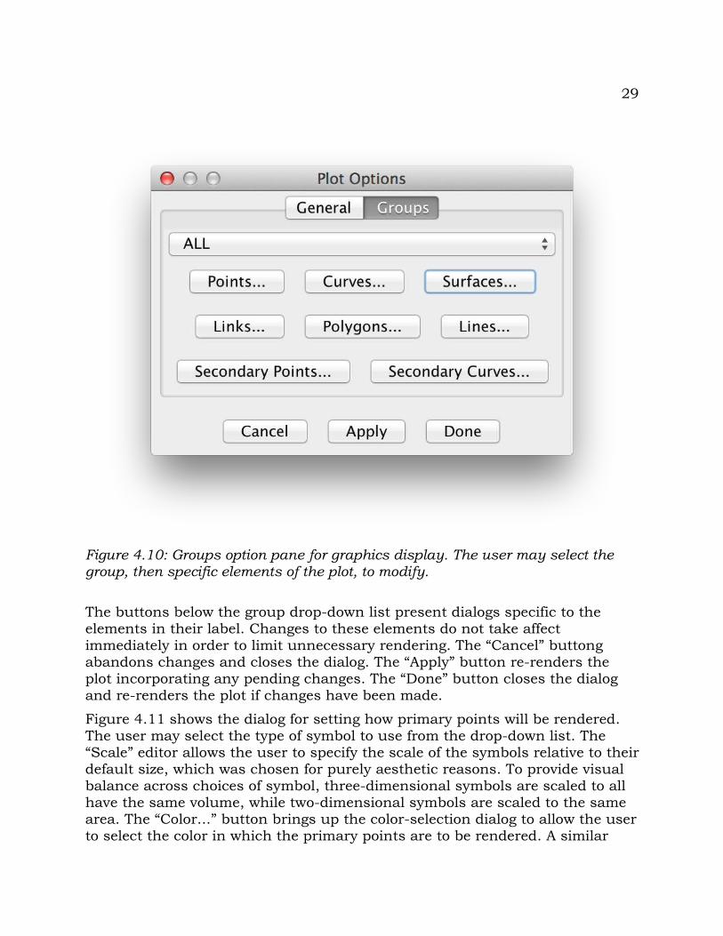
29
The buttons below the group drop-down list present dialogs specific to the elements in their label. Changes to these elements do not take affect immediately in order to limit unnecessary rendering. The “Cancel” buttong abandons changes and closes the dialog. The “Apply” button re-renders the plot incorporating any pending changes. The “Done” button closes the dialog and re-renders the plot if changes have been made.
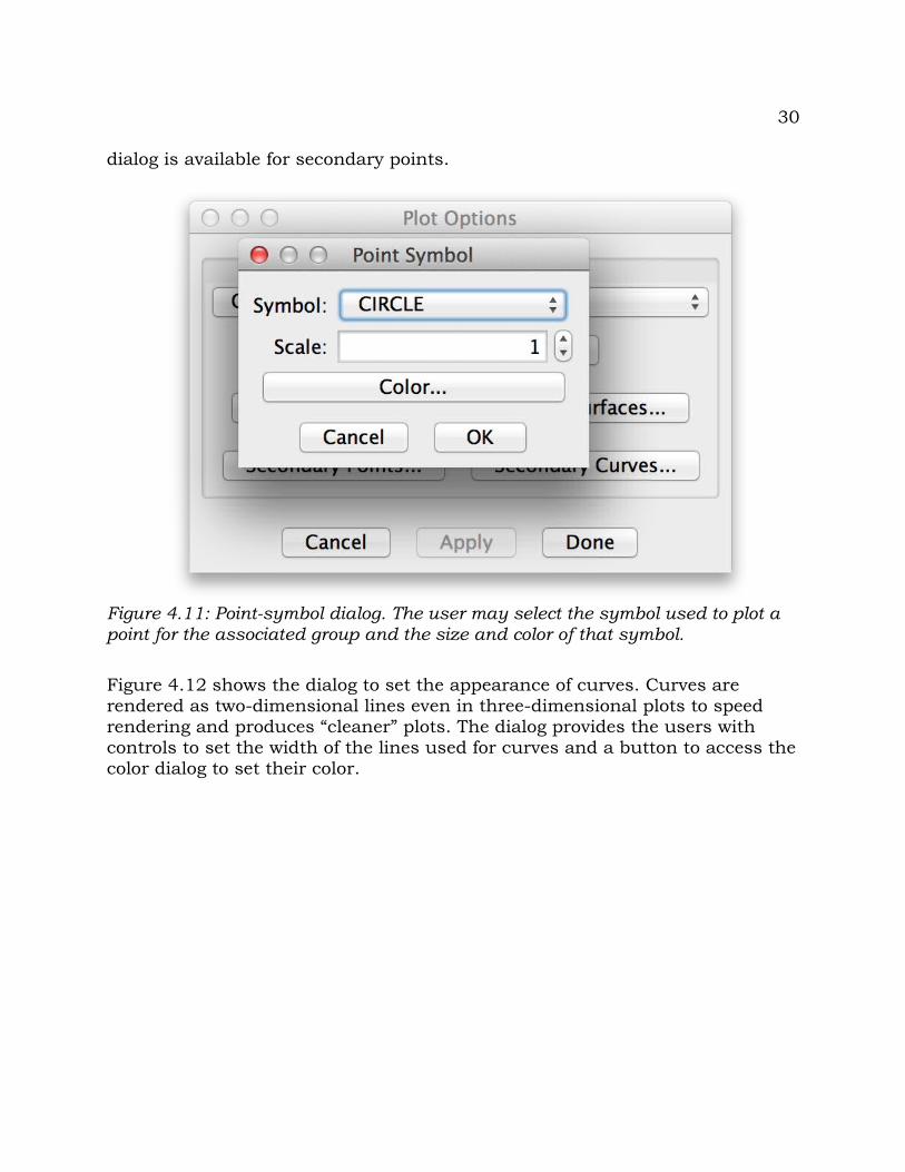
Figure 4.11 shows the dialog for setting how primary points will be rendered. The user may select the type of symbol to use from the drop-down list. The “Scale” editor allows the user to specify the scale of the symbols relative to their default size, which was chosen for purely aesthetic reasons. To provide visual balance across choices of symbol, three-dimensional symbols are scaled to all have the same volume, while two-dimensional symbols are scaled to the same area. The “Color...” button brings up the color-selection dialog to allow the user to select the color in which the primary points are to be rendered. A similar
Figure 4.10: Groups option pane for graphics display. The user may select the group, then specific elements of the plot, to modify.
30
dialog is available for secondary points.
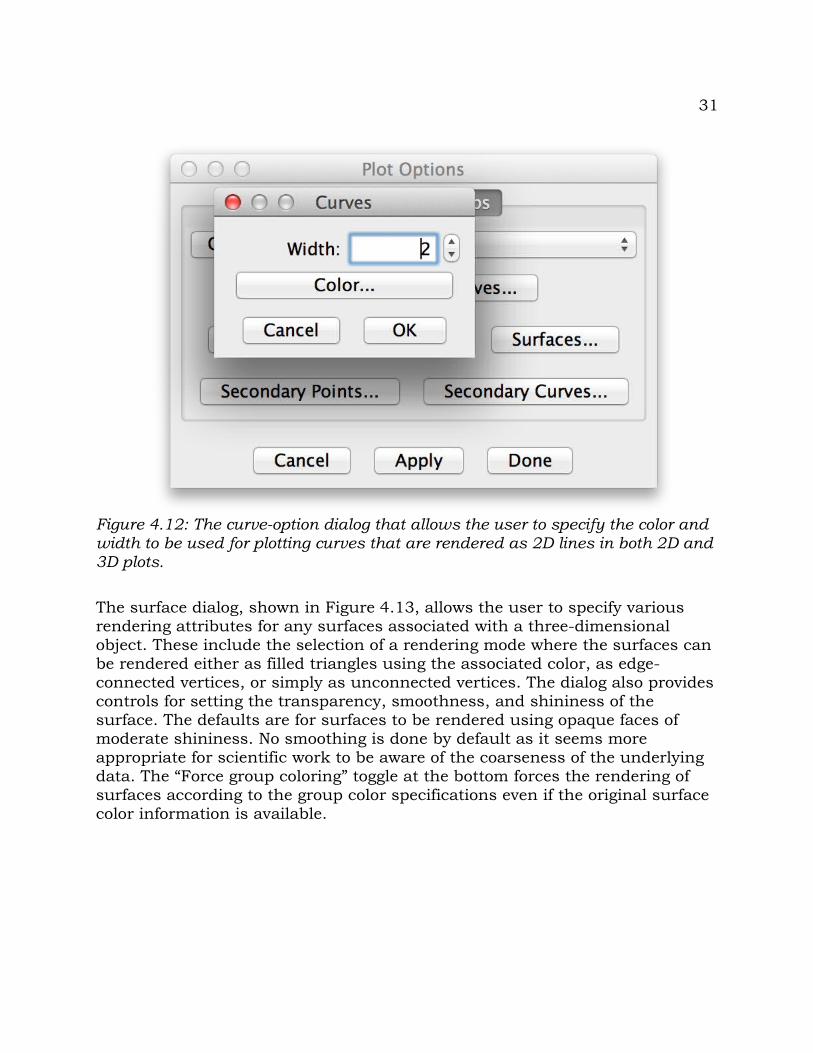
Figure 4.12 shows the dialog to set the appearance of curves. Curves are rendered as two-dimensional lines even in three-dimensional plots to speed rendering and produces “cleaner” plots. The dialog provides the users with controls to set the width of the lines used for curves and a button to access the color dialog to set their color.
Figure 4.11: Point-symbol dialog. The user may select the symbol used to plot a point for the associated group and the size and color of that symbol.
31
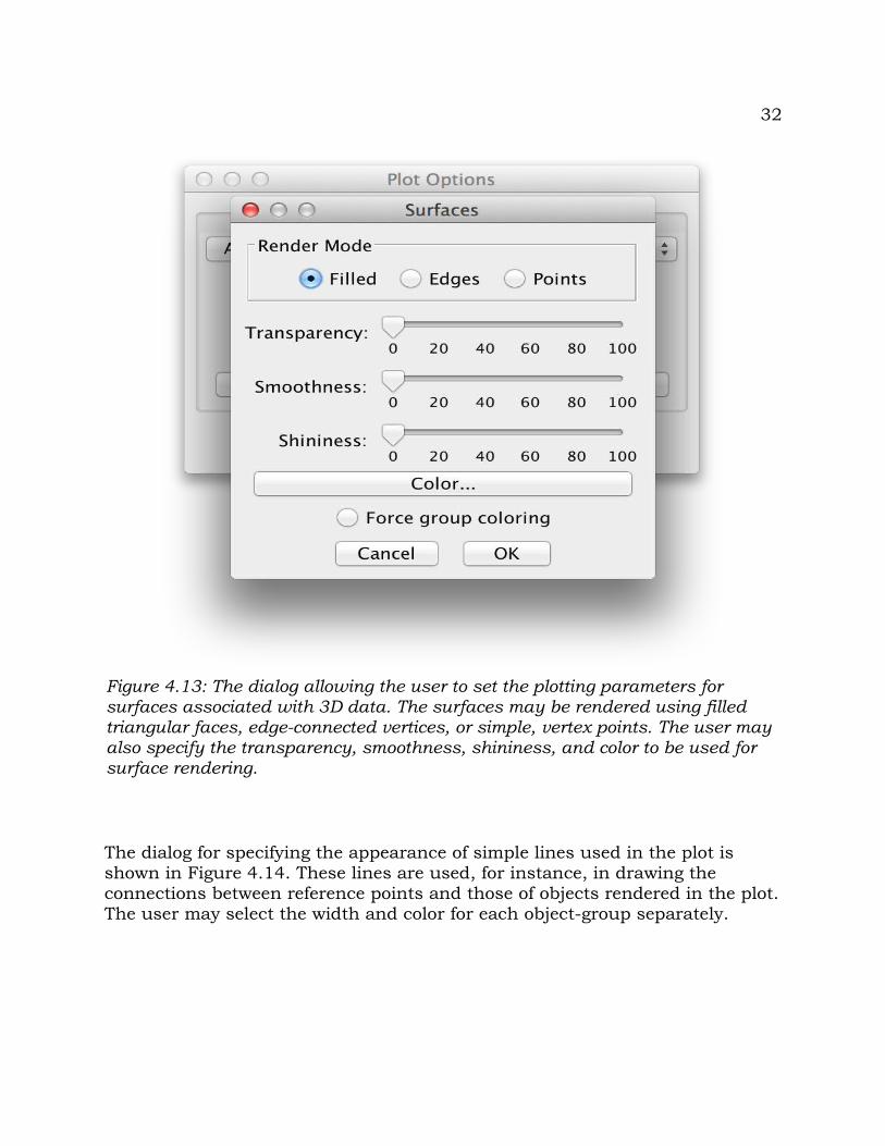
The surface dialog, shown in Figure 4.13, allows the user to specify various rendering attributes for any surfaces associated with a three-dimensional object. These include the selection of a rendering mode where the surfaces can be rendered either as filled triangles using the associated color, as edge-connected vertices, or simply as unconnected vertices. The dialog also provides controls for setting the transparency, smoothness, and shininess of the surface. The defaults are for surfaces to be rendered using opaque faces of moderate shininess. No smoothing is done by default as it seems more appropriate for scientific work to be aware of the coarseness of the underlying data. The “Force group coloring” toggle at the bottom forces the rendering of surfaces according to the group color specifications even if the original surface color information is available.
Figure 4.12: The curve-option dialog that allows the user to specify the color and width to be used for plotting curves that are rendered as 2D lines in both 2D and 3D plots.
32
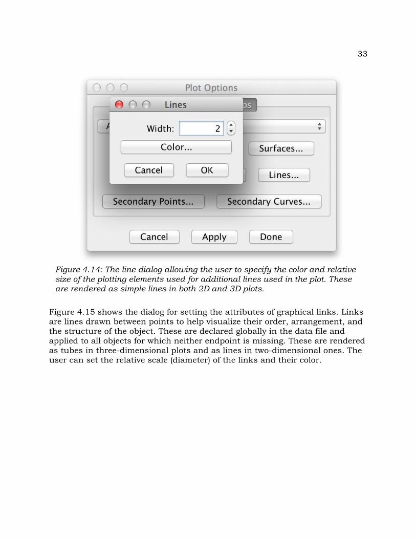
The dialog for specifying the appearance of simple lines used in the plot is shown in Figure 4.14. These lines are used, for instance, in drawing the connections between reference points and those of objects rendered in the plot. The user may select the width and color for each object-group separately.
Figure 4.13: The dialog allowing the user to set the plotting parameters for surfaces associated with 3D data. The surfaces may be rendered using filled triangular faces, edge-connected vertices, or simple, vertex points. The user may also specify the transparency, smoothness, shininess, and color to be used for surface rendering.
33
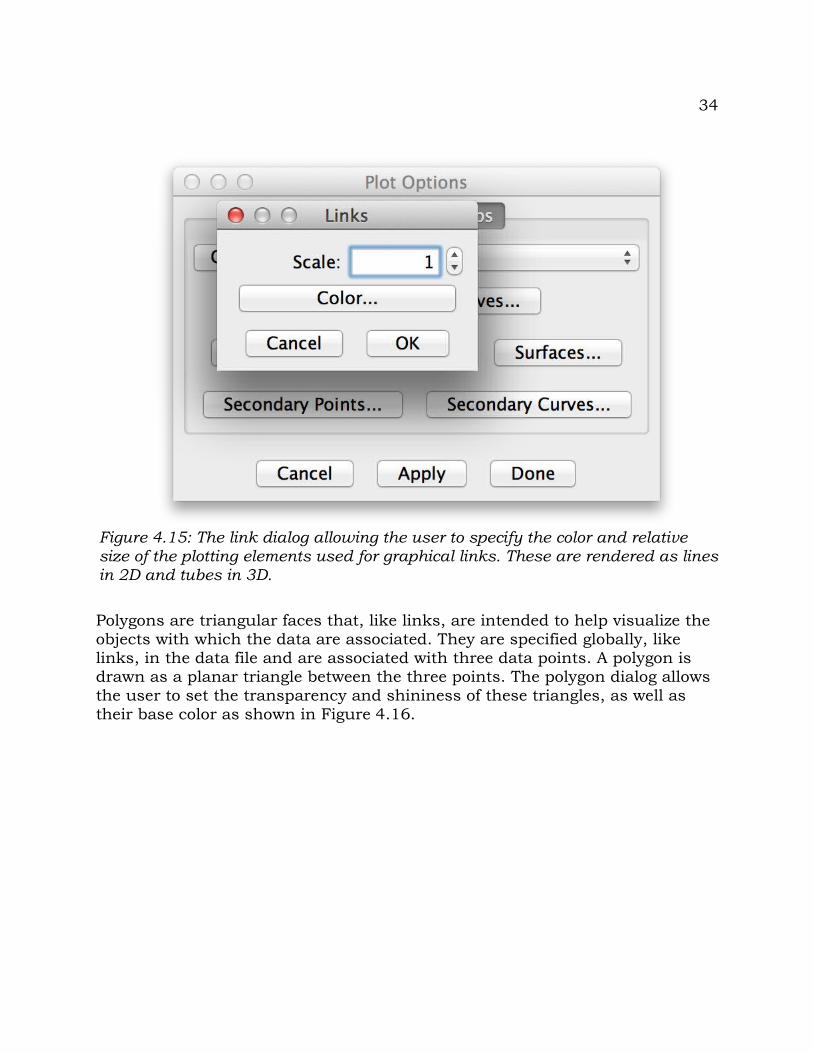
Figure 4.15 shows the dialog for setting the attributes of graphical links. Links are lines drawn between points to help visualize their order, arrangement, and the structure of the object. These are declared globally in the data file and applied to all objects for which neither endpoint is missing. These are rendered as tubes in three-dimensional plots and as lines in two-dimensional ones. The user can set the relative scale (diameter) of the links and their color.
Figure 4.14: The line dialog allowing the user to specify the color and relative size of the plotting elements used for additional lines used in the plot. These are rendered as simple lines in both 2D and 3D plots.
34
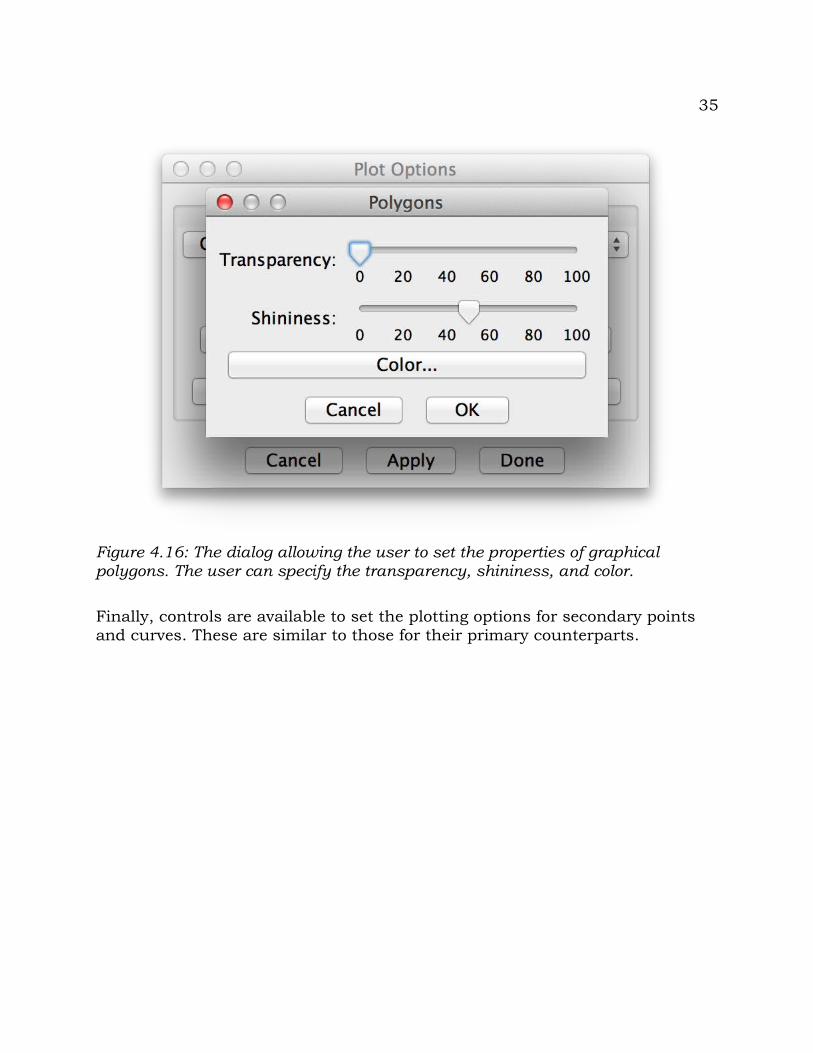
Polygons are triangular faces that, like links, are intended to help visualize the objects with which the data are associated. They are specified globally, like links, in the data file and are associated with three data points. A polygon is drawn as a planar triangle between the three points. The polygon dialog allows the user to set the transparency and shininess of these triangles, as well as their base color as shown in Figure 4.16.
Figure 4.15: The link dialog allowing the user to specify the color and relative size of the plotting elements used for graphical links. These are rendered as lines in 2D and tubes in 3D.
35
Finally, controls are available to set the plotting options for secondary points and curves. These are similar to those for their primary counterparts.
Figure 4.16: The dialog allowing the user to set the properties of graphical polygons. The user can specify the transparency, shininess, and color.

36

37
5 An ExampleNOTE: The figures in this chapter may not reflect the extensive reorganization of the program interface in the latest version. Translation of these examples to the new interface, though, should be straightforward.
To get started with Morpheus et al., let's walk through a simple example. We will read in an example 2D data set distributed with the program. This file consists of data for six ape scapulae – three male lowland gorillas (Gorilla gorilla gorilla) and three male common chimpanzees (Pan troglodytes). The data are the coordinates of ten landmarks digitized from digital images. The images are included with and referenced from the morpheus data file, scapulae.mdt.
We will then look at the data, carry out a generalized Procrustes analysis (GPA), and save the superimposed coordinates to a file in R format for subsequent analysis, say a multivariate t-test. All of the requisite steps should be intuitive.
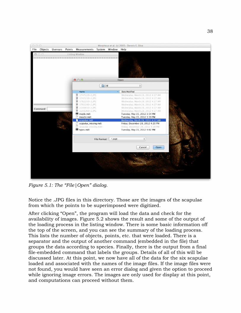
First, we select the “File|Open” menu choice and are presented with a file-selection dialog. Navigate to the morpheus folder and into the data/2d directory. Select “scapulae.mdt” and click “Open” (see Figure 5.1).
38
Notice the .JPG files in this directory. Those are the images of the scapulae from which the points to be superimposed were digitized.
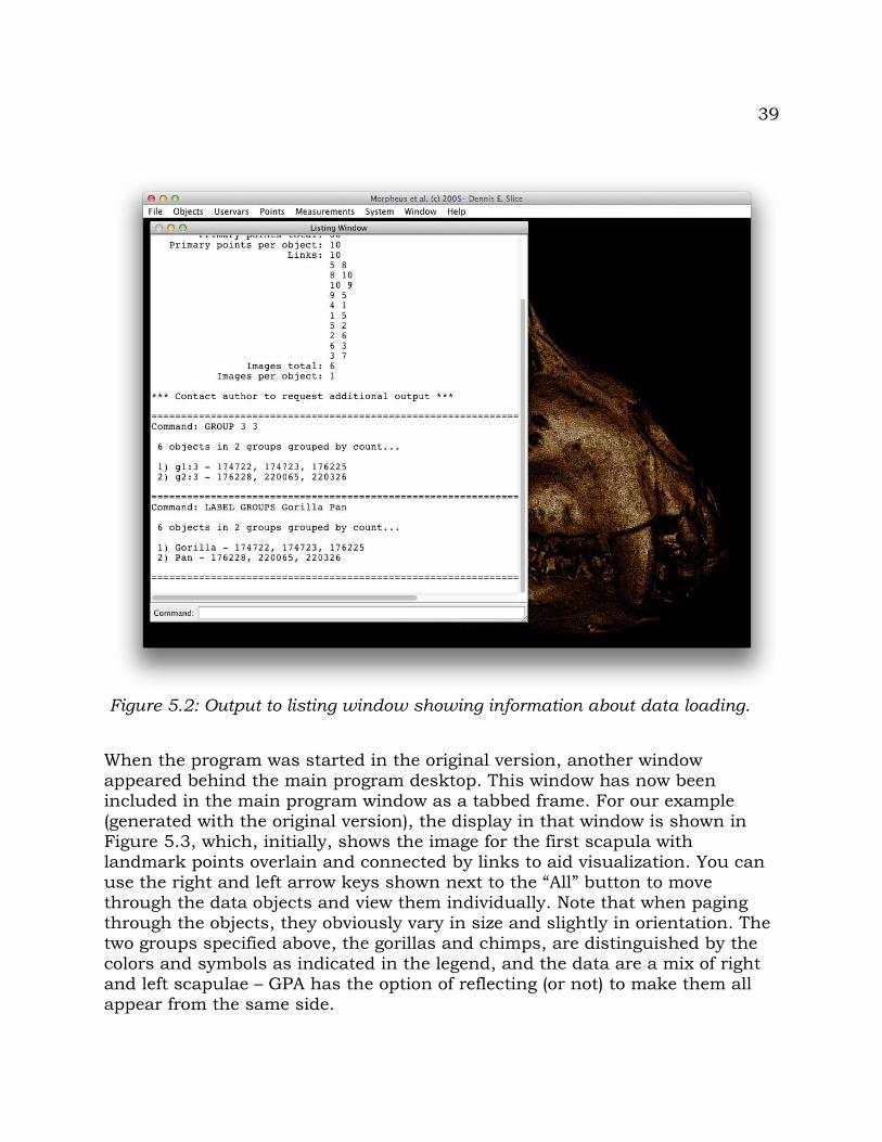
After clicking “Open”, the program will load the data and check for the availability of images. Figure 5.2 shows the result and some of the output of the loading process in the listing window. There is some basic information off the top of the screen, and you can see the summary of the loading process. This lists the number of objects, points, etc. that were loaded. There is a separator and the output of another command (embedded in the file) that groups the data according to species. Finally, there is the output from a final file-embedded command that labels the groups. Details of all of this will be discussed later. At this point, we now have all of the data for the six scapulae loaded and associated with the names of the image files. If the image files were not found, you would have seen an error dialog and given the option to proceed while ignoring image errors. The images are only used for display at this point, and computations can proceed without them.
Figure 5.1: The “File|Open” dialog.
39
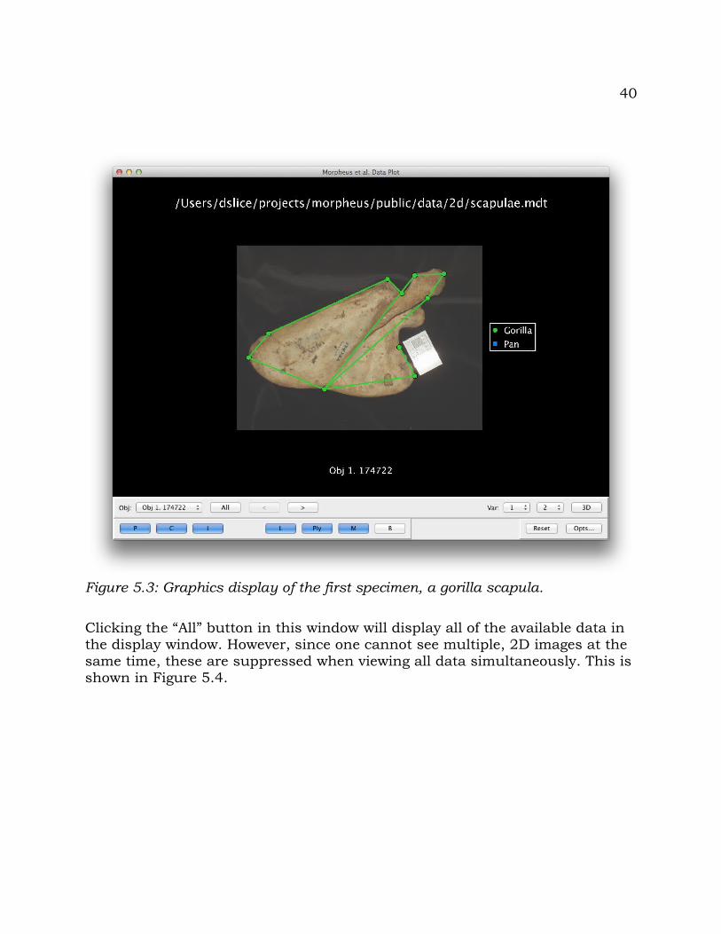
When the program was started in the original version, another window appeared behind the main program desktop. This window has now been included in the main program window as a tabbed frame. For our example (generated with the original version), the display in that window is shown in Figure 5.3, which, initially, shows the image for the first scapula with landmark points overlain and connected by links to aid visualization. You can use the right and left arrow keys shown next to the “All” button to move through the data objects and view them individually. Note that when paging through the objects, they obviously vary in size and slightly in orientation. The two groups specified above, the gorillas and chimps, are distinguished by the colors and symbols as indicated in the legend, and the data are a mix of right and left scapulae – GPA has the option of reflecting (or not) to make them all appear from the same side.
Figure 5.2: Output to listing window showing information about data loading.
40
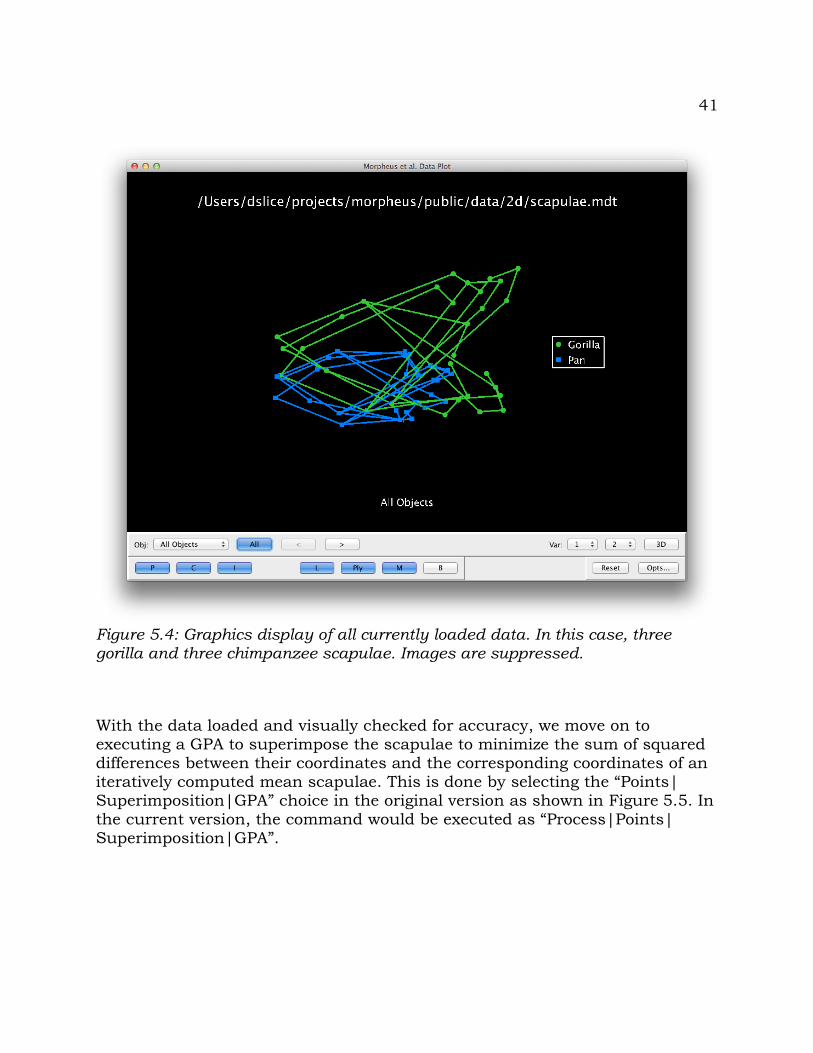
Clicking the “All” button in this window will display all of the available data in the display window. However, since one cannot see multiple, 2D images at the same time, these are suppressed when viewing all data simultaneously. This is shown in Figure 5.4.
Figure 5.3: Graphics display of the first specimen, a gorilla scapula.
41
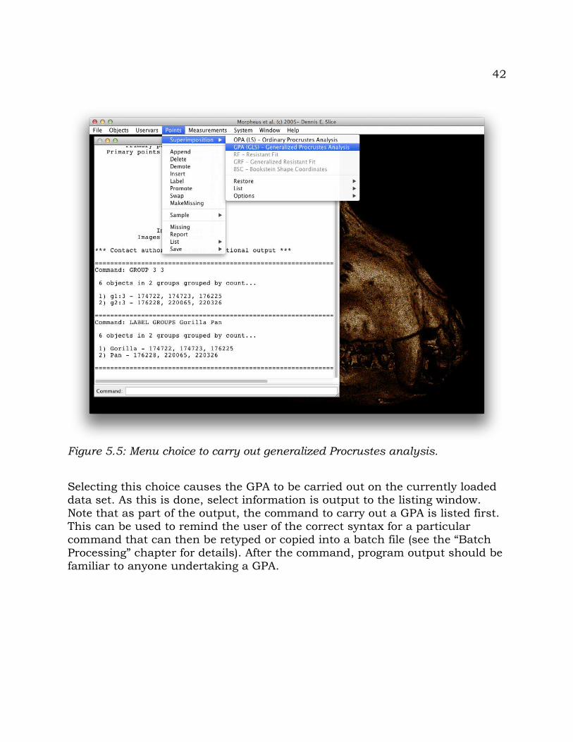
With the data loaded and visually checked for accuracy, we move on to executing a GPA to superimpose the scapulae to minimize the sum of squared differences between their coordinates and the corresponding coordinates of an iteratively computed mean scapulae. This is done by selecting the “Points|Superimposition|GPA” choice in the original version as shown in Figure 5.5. In the current version, the command would be executed as “Process|Points|Superimposition|GPA”.
Figure 5.4: Graphics display of all currently loaded data. In this case, three gorilla and three chimpanzee scapulae. Images are suppressed.
42
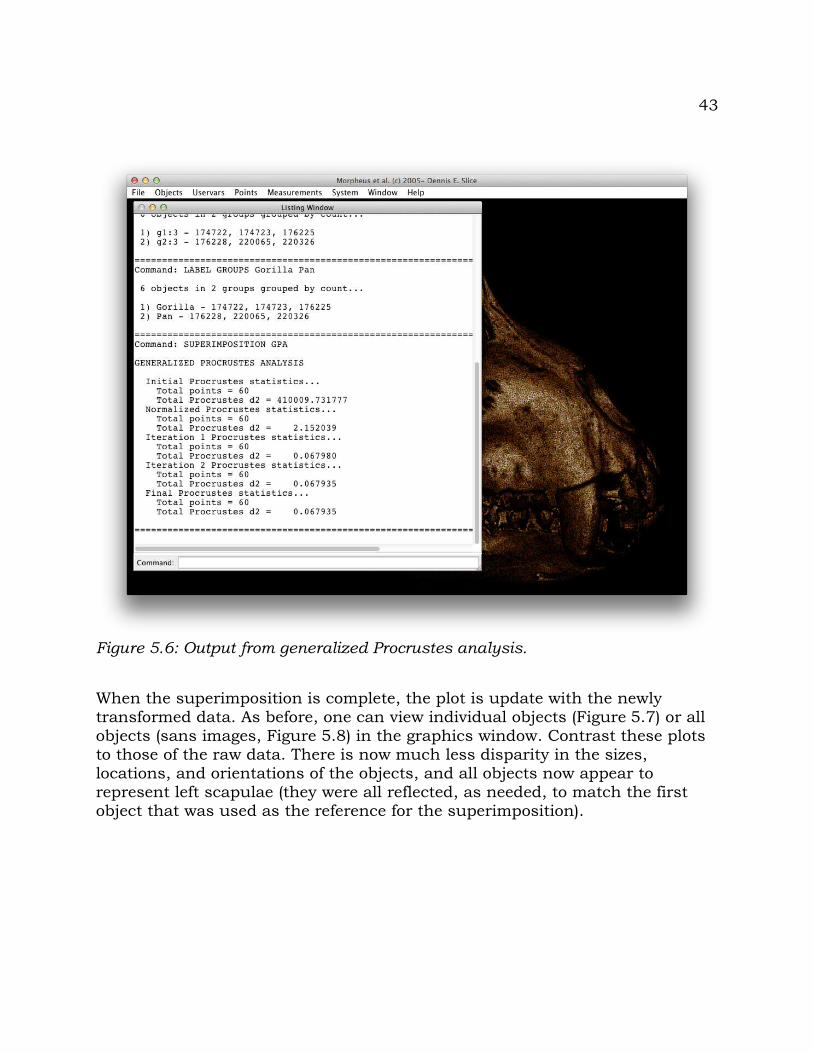
Selecting this choice causes the GPA to be carried out on the currently loaded data set. As this is done, select information is output to the listing window. Note that as part of the output, the command to carry out a GPA is listed first. This can be used to remind the user of the correct syntax for a particular command that can then be retyped or copied into a batch file (see the “Batch Processing” chapter for details). After the command, program output should be familiar to anyone undertaking a GPA.
Figure 5.5: Menu choice to carry out generalized Procrustes analysis.
43
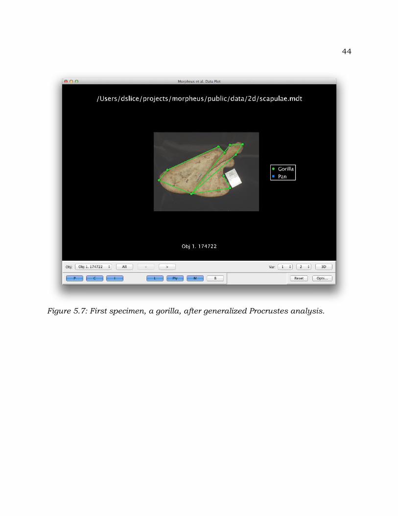
When the superimposition is complete, the plot is update with the newly transformed data. As before, one can view individual objects (Figure 5.7) or all objects (sans images, Figure 5.8) in the graphics window. Contrast these plots to those of the raw data. There is now much less disparity in the sizes, locations, and orientations of the objects, and all objects now appear to represent left scapulae (they were all reflected, as needed, to match the first object that was used as the reference for the superimposition).
Figure 5.6: Output from generalized Procrustes analysis.
44
Figure 5.7: First specimen, a gorilla, after generalized Procrustes analysis.
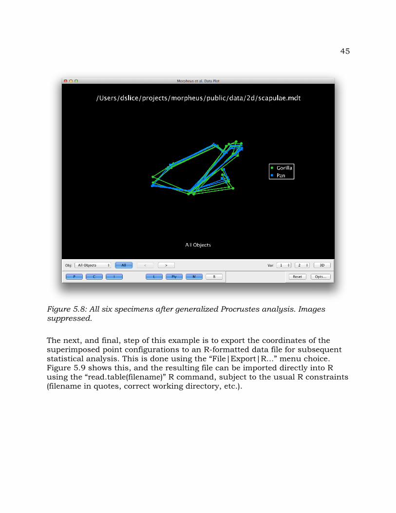
45
The next, and final, step of this example is to export the coordinates of the superimposed point configurations to an R-formatted data file for subsequent statistical analysis. This is done using the “File|Export|R...” menu choice. Figure 5.9 shows this, and the resulting file can be imported directly into R using the “read.table(filename)” R command, subject to the usual R constraints (filename in quotes, correct working directory, etc.).
Figure 5.8: All six specimens after generalized Procrustes analysis. Images suppressed.
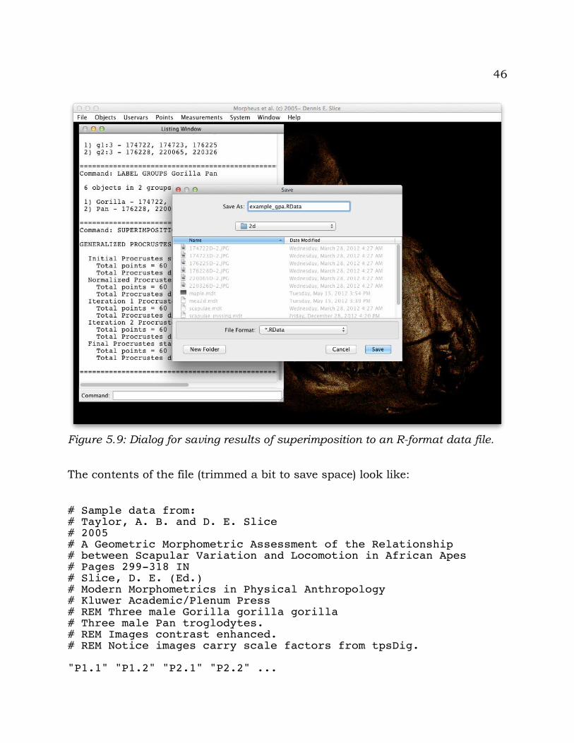
46
The contents of the file (trimmed a bit to save space) look like:
# Sample data from:# Taylor, A. B. and D. E. Slice# 2005# A Geometric Morphometric Assessment of the Relationship# between Scapular Variation and Locomotion in African Apes# Pages 299-318 IN# Slice, D. E. (Ed.)# Modern Morphometrics in Physical Anthropology# Kluwer Academic/Plenum Press# REM Three male Gorilla gorilla gorilla# Three male Pan troglodytes.# REM Images contrast enhanced.# REM Notice images carry scale factors from tpsDig.
"P1.1" "P1.2" "P2.1" "P2.2" ...
Figure 5.9: Dialog for saving results of superimposition to an R-format data file.
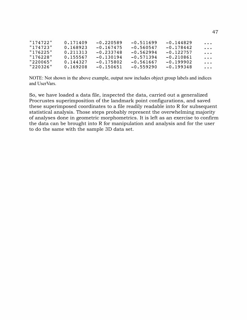
47
"174722" 0.171409 -0.220589 -0.511699 -0.144829 ..."174723" 0.168923 -0.167475 -0.560547 -0.178442 ..."176225" 0.211313 -0.233748 -0.562994 -0.122757 ..."176228" 0.155567 -0.130194 -0.571394 -0.210861 ..."220065" 0.144327 -0.175802 -0.561667 -0.199902 ..."220326" 0.169208 -0.150651 -0.559290 -0.199348 ...
NOTE: Not shown in the above example, output now includes object group labels and indices and UserVars.
So, we have loaded a data file, inspected the data, carried out a generalized Procrustes superimposition of the landmark point configurations, and saved these superimposed coordinates to a file readily readable into R for subsequent statistical analysis. Those steps probably represent the overwhelming majority of analyses done in geometric morphometrics. It is left as an exercise to confirm the data can be brought into R for manipulation and analysis and for the user to do the same with the sample 3D data set.

48
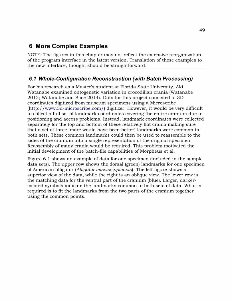
49
6 More Complex ExamplesNOTE: The figures in this chapter may not reflect the extensive reorganization of the program interface in the latest version. Translation of these examples to the new interface, though, should be straightforward.
6.1 Whole-Configuration Reconstruction (with Batch Processing)For his research as a Master's student at Florida State University, Aki Watanabe examined ontogenetic variation in crocodilian crania (Watanabe 2012; Watanabe and Slice 2014). Data for this project consisted of 3D coordinates digitized from museum specimens using a Microscribe (http://www.3d-microscribe.com/) digitizer. However, it would be very difficult to collect a full set of landmark coordinates covering the entire cranium due to positioning and access problems. Instead, landmark coordinates were collected separately for the top and bottom of these relatively flat crania making sure that a set of three (more would have been better) landmarks were common to both sets. These common landmarks could then be used to reassemble to the sides of the cranium into a single representation of the original specimen. Reassembly of many crania would be required. This problem motivated the initial development of the batch-file capabilities of Morpheus et al.
Figure 6.1 shows an example of data for one specimen (included in the sample data sets). The upper row shows the dorsal (green) landmarks for one specimen of American alligator (Alligator mississippiensis). The left figure shows a superior view of the data, while the right is an oblique view. The lower row is the matching data for the ventral part of the cranium (blue). Larger, darker-colored symbols indicate the landmarks common to both sets of data. What is required is to fit the landmarks from the two parts of the cranium together using the common points.
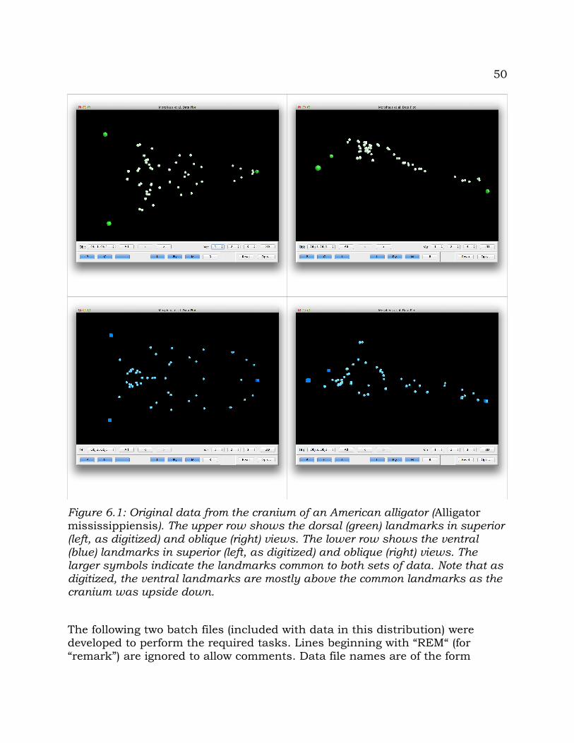
50
Figure 6.1: Original data from the cranium of an American alligator (Alligator mississippiensis). The upper row shows the dorsal (green) landmarks in superior (left, as digitized) and oblique (right) views. The lower row shows the ventral (blue) landmarks in superior (left, as digitized) and oblique (right) views. The larger symbols indicate the landmarks common to both sets of data. Note that as digitized, the ventral landmarks are mostly above the common landmarks as the cranium was upside down.
The following two batch files (included with data in this distribution) were developed to perform the required tasks. Lines beginning with “REM“ (for “remark”) are ignored to allow comments. Data file names are of the form
51
“unique_id-dors.mdt” and “unique_id-vent.mdt”, where “unique-id” is the unique identifier indicating an individual specimen and “-dors” and “-vent” indicate files with dorsal and ventral landmark coordinates.
The first file defines variables for the unique identifiers used in the datafile names. It then invokes a second batch file where the variables are used in the relative complex set of tasks needed to carry out the desired operations. Variables can be redefined and the second batch file called as many times as needed from within the first batch file:
REM Morpheus et al. batch processing example
REM This is an example batch file that defines REM variables representing unique text in the names REM of files to be processed.
REM Here is where we define the unique parts of the REM file name(s).define $fn$ allmis_A_AMNH9043
REM Now we call the merging commands that willREM substitute "allmis_A_AMNH9043" for "$fn$"batch 02_batch_merge.btc
REM Repeat as needed. E.g.,...REM define $fn$ allmis_A_AMNH9047REM batch 02_batch_merge.btcREM define $fn$ allmis_A_AMNH9127REM batch 02_batch_merge.btc
In the second batch file, the value of the variable defined in the first bath file is used to carry out the desired tasks. Ellipses (“...”) indicates lines deleted to save space.
REM Morpheus et al. batch processing example.
REM $fn$ has been defined in the calling batch fileREM and used to identify individual files to beREM processed. In this case, we have dorsal and ventralREM landmark coordinates from the same cranium stored in.REM separate files. The first three points in both filesREM are homologous. We need to fill out both sets soREM all corresponding points are homologous.
REM NOTE: the APPEND and INSERT commands have changed REM from earlier versions. Those were of the form:REM APPEND p MISSING o 1
52
REM INSERT p 4 MISSING o 1REM As there is no common scenario in which one couldREM reasonably provide actual coordinates, the specificationREM of "MISSING" was deemed entirely unnecessary. The newREM syntax for these commands, used below, is of the form:REM APPEND p o 1REM INSERT p 4 o 1
REM Open the first file and append the second.REM We now have two objects with different numbers of points.OPEN $fn$-dors.mdtAPPEND $fn$-vent.mdt
REM Fill out both data sets.REM Append ventral points as missing to dorsal data.APPEND p o 1 APPEND p o 1APPEND p o 1...APPEND p o 1APPEND p o 1APPEND p o 1
REM Insert dorsal points at position 4 (the first three are REM homologous) as missing to ventral data.INSERT p 4 o 2 INSERT p 4 o 2INSERT p 4 o 2...INSERT p 4 o 2INSERT p 4 o 2 INSERT p 4 o 2
REM The following approach is much more efficient REM than demoting individual points.REM Demote all 134 pointsdemote p *REM Now, promote the common points (1-3) in both.promote p 1promote p 2promote p 3
REM GPA the two configurations.REM Fitting will only use the remaining primary pointsREM 1-3 which should match nearly perfectly as they areREM the same points from the same cranium.REM Because the common points formed a planar triangleREM (not the best choice for 3D data), we must not allow REM reflections.super set allowreflections falsesuper gpa
53
REM Restore the configurations to their original size.super restore scale
REM Compute the grand mean of the two objects.REM The grand mean is a reconstruction of theREM entire configuration of cranial landmarks REM from the original two files.
REM Both configurations have the first three points inREM common, which should differ only by digitizing error.REM The remaining are all data paired with MISSING values.REM Hence, the mean will be those original coordinatesREM re-aligned by the common points.OBJECTS SAVE MEANS GRAND $fn$_merged.mdt
REM Reopen and rename grand mean for later mergingREM of many crania into a single data set. Otherwise, REM they all have the same object name "grand_mean"OPEN $fn$_merged.mdtOBJECT RENAME 1 $fn$SAVEAS $fn$_merged.mdt
REM That's it. Will return to the calling batch fileREM which can redefine $fn$ to process data for anotherREM cranium.
The following is some heavily edited batch-file output. The batch level and line number are output prior to the execution of a batch line command. The batch level is indicated by the number of periods preceding the line number - '.' first-level batch file, '..' second-level batch file, etc. Remark lines are echoed to the output. Blank lines are counted, but ignored. In the following, ellipses (“...”) indicated lines deleted to save space.
================================================================Command: BATCH 01_batch_def.btc
.Processing batch file /Users/myaccount/data/batch/01_batch_def.btc
================================================================.Batch Line 1Command: REM Morpheus et al. batch processing example
Morpheus et al. batch processing example
================================================================.Batch Line 3
54
Command: REM This is an example batch file that defines
This is an example batch file that defines
...
================================================================.Batch Line 9Command: DEFINE $fn$ allmis_A_AMNH9043
$fn$ = allmis_A_AMNH9043
================================================================.Batch Line 11Command: REM Now we call the merging commands that will
Now we call the merging commands that will
================================================================.Batch Line 12Command: REM substitute "allmis_A_AMNH9043" for "allmis_A_AMNH9043"
substitute "allmis_A_AMNH9043" for "allmis_A_AMNH9043"
================================================================.Batch Line 13Command: BATCH 02_batch_merge.btc
..Processing batch file /Users/myaccount/data/batch/02_batch_merge.btc
================================================================..Batch Line 1Command: REM Morpheus et al. batch processing example.
Morpheus et al. batch processing example.
...
================================================================..Batch Line 13Command: OPEN allmis_A_AMNH9043-dors.mdt
1 3D object loaded from /Users/myaccount/data/batch/allmis_A_AMNH9043-dors.mdt
Primary points total: 78 Primary points missing: 23 Primary points per object: 78
55
*** Contact author to request additional output ***
...
================================================================
..Processing complete of batch file /Users/myaccount/data/batch/02_batch_merge.btc
================================================================.Batch Line 15Command: REM Repeat as needed. E.g.,...
Repeat as needed. E.g.,...
...
================================================================
.Processing complete of batch file /Users/myaccount/data/batch/01_batch_def.btc
================================================================
Figure 6.2 shows the results of the above process. The image on the left is not produced by the batch files, but was, instead, generated by hand to illustrate an intermediate stage in data merging. It shows the dorsal (green) and ventral (blue) datasets as two objects fit together by their common landmarks (larger symbols). The image on the right is the final object that is the average of the two objects in the left image that was saved as single, reconstructed specimen. At this point, the common points are still classified as primary points while those unique to either the dorsal or ventral components are still classified as secondary points. Promoting all points to primary status would be the next step prior to further morphometric analysis.
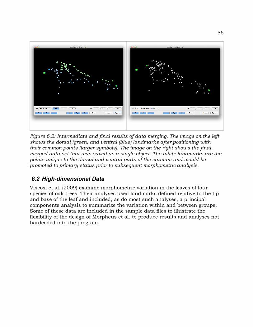
56
Figure 6.2: Intermediate and final results of data merging. The image on the left shows the dorsal (green) and ventral (blue) landmarks after positioning with their common points (larger symbols). The image on the right shows the final, merged data set that was saved as a single object. The white landmarks are the points unique to the dorsal and ventral parts of the cranium and would be promoted to primary status prior to subsequent morphometric analysis.
6.2 High-dimensional DataViscosi et al. (2009) examine morphometric variation in the leaves of four species of oak trees. Their analyses used landmarks defined relative to the tip and base of the leaf and included, as do most such analyses, a principal components analysis to summarize the variation within and between groups. Some of these data are included in the sample data files to illustrate the flexibility of the design of Morpheus et al. to produce results and analyses not hardcoded into the program.
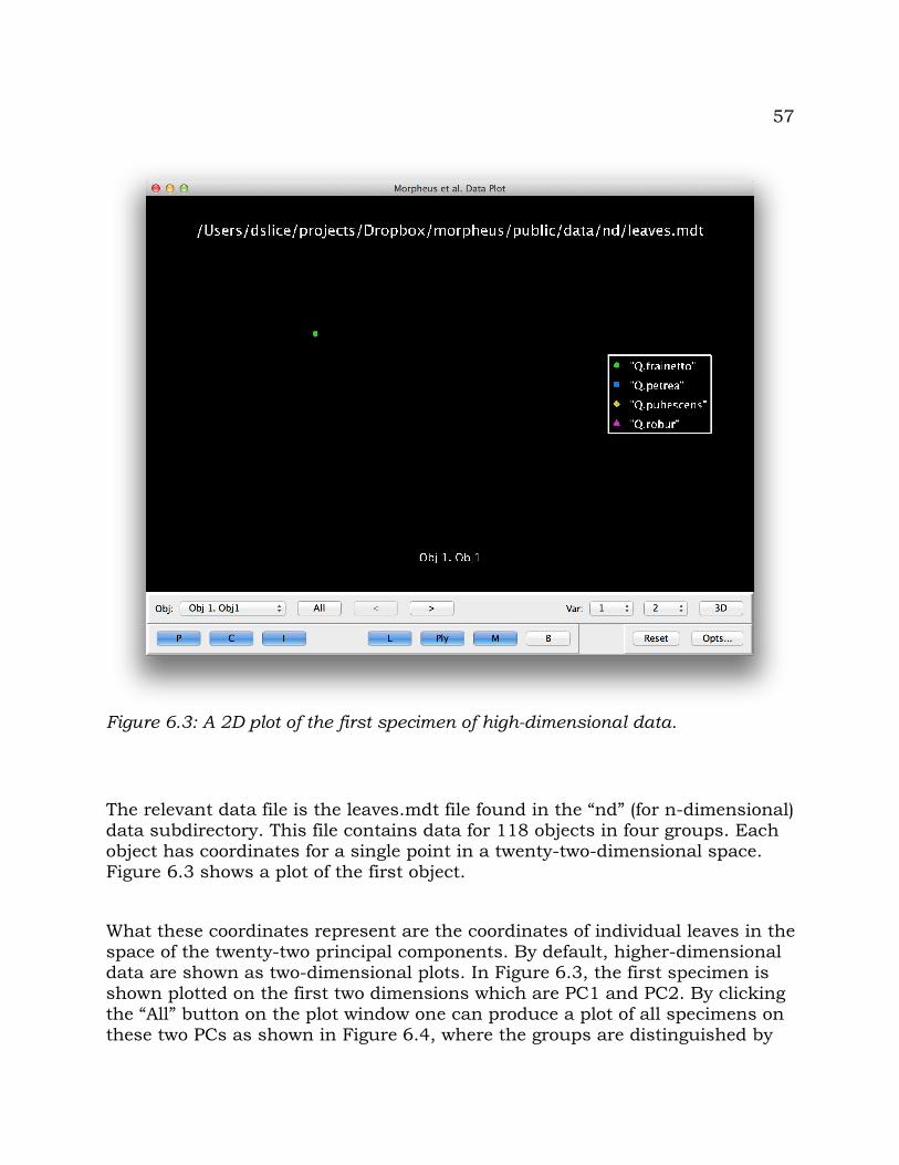
57
The relevant data file is the leaves.mdt file found in the “nd” (for n-dimensional) data subdirectory. This file contains data for 118 objects in four groups. Each object has coordinates for a single point in a twenty-two-dimensional space. Figure 6.3 shows a plot of the first object.
What these coordinates represent are the coordinates of individual leaves in the space of the twenty-two principal components. By default, higher-dimensional data are shown as two-dimensional plots. In Figure 6.3, the first specimen is shown plotted on the first two dimensions which are PC1 and PC2. By clicking the “All” button on the plot window one can produce a plot of all specimens on these two PCs as shown in Figure 6.4, where the groups are distinguished by
Figure 6.3: A 2D plot of the first specimen of high-dimensional data.
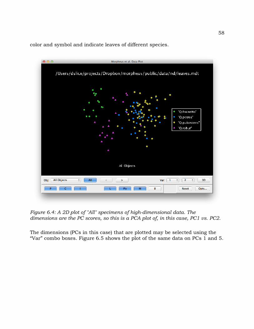
58
color and symbol and indicate leaves of different species.
The dimensions (PCs in this case) that are plotted may be selected using the “Var” combo boxes. Figure 6.5 shows the plot of the same data on PCs 1 and 5.
Figure 6.4: A 2D plot of "All" specimens of high-dimensional data. The dimensions are the PC scores, so this is a PCA plot of, in this case, PC1 vs. PC2.
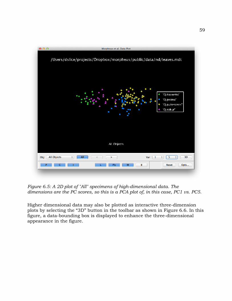
59
Higher dimensional data may also be plotted as interactive three-dimension plots by selecting the “3D” button in the toolbar as shown in Figure 6.6. In this figure, a data-bounding box is displayed to enhance the three-dimensional appearance in the figure.
Figure 6.5: A 2D plot of "All" specimens of high-dimensional data. The dimensions are the PC scores, so this is a PCA plot of, in this case, PC1 vs. PC5.

60
Three-dimensional plots default to plotting dimensions one, two, and three for higher-dimensional data, but these can be changed using the “Var” combo boxes. For two-dimensional data, the third axes defaults to “null” so that the user has a rotatable, flat representation of the data, but, again, this can be changed to any combination of available axes.
6.3 ReferencesViscosi, V., P. Fortini, D. E. Slice, A. Loy, and C. Blasi. 2009. “Geometric Morphometric Analyses of Leaf Variation in Four Oak Species of the Subgenus Quercus (Fagaceae).” Plant Biosystems - An International Journal Dealing with All Aspects of Plant Biology 143 (3): 575–587.
Figure 6.6: A 3D plot of "All" specimens of high-dimensional data. The dimensions are the PC scores, so this is a PCA plot of, in this case, PC1 vs. PC2 vs. PC3. A bounding box is shown to enhance the 3D appearance of the plot.

61
doi:10.1080/11263500902775277.
Watanabe, A. 2012. The ontogeny of cranial morphology in extant crocodilians and its phylogenetic utility: a geometric morphometric approach. MS Thesis, Florida State University.
Watanabe, A, and D E Slice. 2014. The Utility of Cranial Ontogeny for Phylogenetic Inference: A Case Study in Crocodylians Using Geometric Morphometrics. Journal of Evolutionary Biology 27 (6): 1078–92. doi:10.1111/jeb.12382.

62
63
7 Commands
Program commands may be entered in the command-line area of the text pane. The menu system simply provides an easy method for the construction of these commands, which are then submitted to the program for processing. In many cases, the selection of a menu item will bring up a dialog with a skeleton of the command presented for editing by the user.
The menu system for this version of Morpheus et al. has been extensively revised. Submenus are now grouped based on the operations contained therein – viewing, editing, processing, etc. Within each submenu, commands are organized according to the type of data to which they are relevant – objects, points, etc.
The submenus of the main menu (Figure 7.1) are presented below, as are their commands and lower-level submenus. See the “What's new?” section of “Introduction” chapter for an explanation of the use of the iSeq command parameter.
7.1 File
Figure 7.1: The main menu.
Figure 7.2: The “File” submenu.

64
The “File” submenu (Figure 7.2) provides access to choices and submenus related to reading and writing data, log, and other files.
7.1.1 File|Open...Command: OPEN filename
Selecting the “File|Open...” menu choice presents the user with a file-selection dialog box highlighting files with the .mdt extension. This is the default extension used for Morpheus data files, but this is not enforced, so the user can select other files by choosing the “All Files” file format.Once selected, the program attempts to load the specified data file. Example output is shown below. The warning notes that it has been detected that the file contains older formatting tags associated with the original Morpheus et al. program (see the “Morpheus Data Files (.mdt)” chapter). The number of objects loaded, their dimensionality, and file name are shown next. This is followed by a summary of that data: number of primary points, primary points per object (which can be variable), any visual links that were specified and their definitions, the total number of images, and the number of images per object (usually one, but not strictly required).After the initial data is loaded, any commands embedded in the data file are applied to the data. In this case, the six objects were grouped into two groups of three and these groups given more meaningful labels.
================================================================Command: OPEN scapulae.mdt
WARNING: Converting old-format, embedded LABEL command.
6 2D objects loaded from /Users/myaccount/data/2d/scapulae.mdt
Primary points total: 60 Primary points per object: 10 Links: 10 5 8 8 10 10 9 9 5 4 1 1 5 5 2 2 6 6 3 3 7 Images total: 6 Images per object: 1
*** Contact author to request additional output ***
65
================================================================Command: GROUP 3 3
6 objects in 2 groups grouped by count...
1) g1:3 - 174722, 174723, 176225 2) g2:3 - 176228, 220065, 220326
================================================================Command: LABEL GROUPS Gorilla Pan
6 objects in 2 groups grouped by count...
1) Gorilla - 174722, 174723, 176225 2) Pan - 176228, 220065, 220326
7.1.2 File|Append...Command: APPEND FILE filename
The “File|Append...” menu choice allows one Morpheus data set to be appended to the current object list. The user is presented with a file-selection dialog box and the appropriate command-line command generated. An error is displayed if there is not an existing object list to which to append the new data.
A good use of this feature is to save a specimen-specific set of graphical links to a file, then append those to different data files related to that type of specimen. For instance, one might have a link file for turtles or human face scans, as long as all data sets contained the same landmarks in the same order.
If the data are grouped, an error occurs and the append routine aborted. There is no clear action to take with respect to how to introduce new data into a grouped data structure.
Finally, note the “FILE” term is not required, but should be used. The default action of the APPEND command is to append a data file to a current data list, but there are other APPEND commands that need to be distinguished. For instance, one can APPEND points to objects.
7.1.3 File|Save As...Command: SAVEAS filename
The “File|Save As...” menu choice allows for saving the current data to a specified file. This choice opens the usual file-selection dialog for saving files
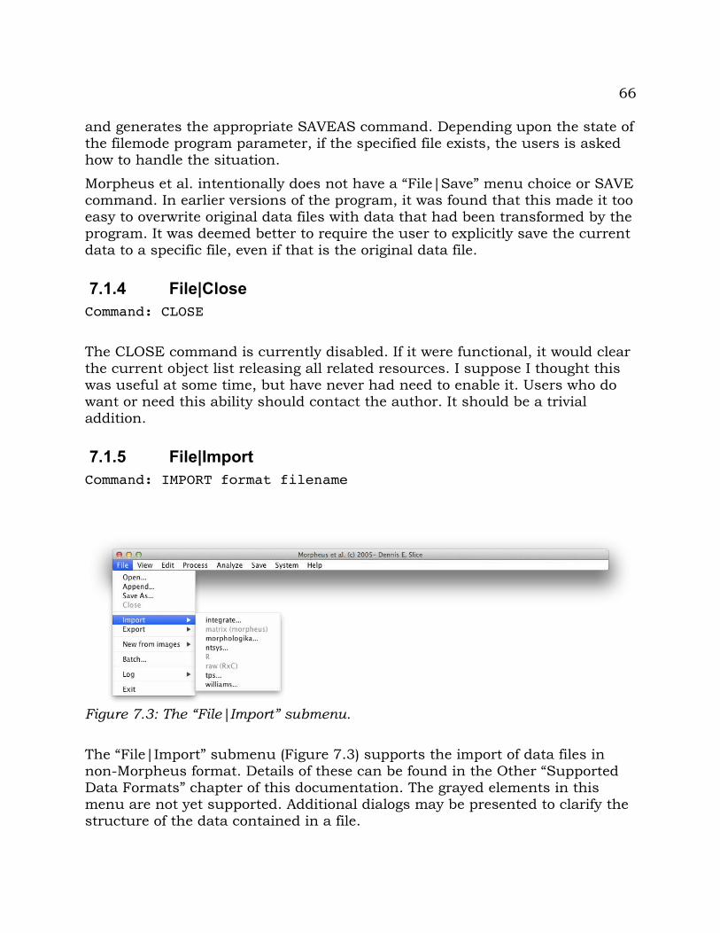
66
and generates the appropriate SAVEAS command. Depending upon the state of the filemode program parameter, if the specified file exists, the users is asked how to handle the situation.
Morpheus et al. intentionally does not have a “File|Save” menu choice or SAVE command. In earlier versions of the program, it was found that this made it too easy to overwrite original data files with data that had been transformed by the program. It was deemed better to require the user to explicitly save the current data to a specific file, even if that is the original data file.
7.1.4 File|CloseCommand: CLOSE
The CLOSE command is currently disabled. If it were functional, it would clear the current object list releasing all related resources. I suppose I thought this was useful at some time, but have never had need to enable it. Users who do want or need this ability should contact the author. It should be a trivial addition.
7.1.5 File|ImportCommand: IMPORT format filename
The “File|Import” submenu (Figure 7.3) supports the import of data files in non-Morpheus format. Details of these can be found in the Other “Supported Data Formats” chapter of this documentation. The grayed elements in this menu are not yet supported. Additional dialogs may be presented to clarify the structure of the data contained in a file.
Figure 7.3: The “File|Import” submenu.
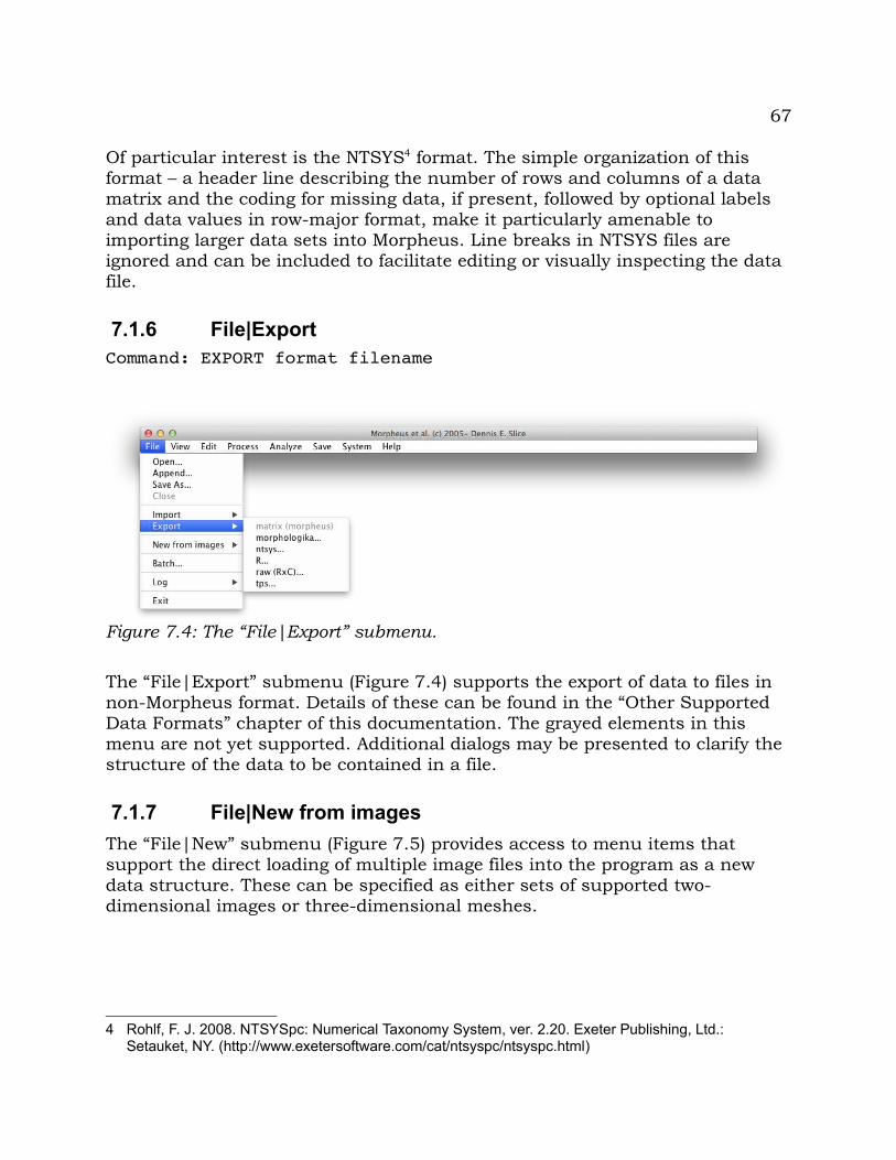
67
Of particular interest is the NTSYS4 format. The simple organization of this format – a header line describing the number of rows and columns of a data matrix and the coding for missing data, if present, followed by optional labels and data values in row-major format, make it particularly amenable to importing larger data sets into Morpheus. Line breaks in NTSYS files are ignored and can be included to facilitate editing or visually inspecting the data file.
7.1.6 File|ExportCommand: EXPORT format filename
The “File|Export” submenu (Figure 7.4) supports the export of data to files in non-Morpheus format. Details of these can be found in the “Other Supported Data Formats” chapter of this documentation. The grayed elements in this menu are not yet supported. Additional dialogs may be presented to clarify the structure of the data to be contained in a file.
7.1.7 File|New from imagesThe “File|New” submenu (Figure 7.5) provides access to menu items that support the direct loading of multiple image files into the program as a new data structure. These can be specified as either sets of supported two-dimensional images or three-dimensional meshes.
4 Rohlf, F. J. 2008. NTSYSpc: Numerical Taxonomy System, ver. 2.20. Exeter Publishing, Ltd.: Setauket, NY. (http://www.exetersoftware.com/cat/ntsyspc/ntsyspc.html)
Figure 7.4: The “File|Export” submenu.

68
7.1.8 File|New from images|2D...Command: NEW 2D filename [filename ...]
The “File|New from images|2D...” menu choice opens a file-selection dialog that allows the user to select multiple two-dimensional images from which to build a new main data structure. Images in any supported format are made available in the dialog. Selecting images and clicking the “Open” button replaces the currently loaded data with a new data set including the selected images. These data can then be saved or exported to a Morpheus et al. or other format file. In the latter case, exporting to a tps file would be similar to using the tpsUtil function to create a tps file from images for use in tpsDig. Example output is shown below.
================================================================Command: NEW 2D 174722D-2.JPG 176225D-2.JPG 220065D-2.JPG
Creating new data set...Object added with image 174722D-2.JPGObject added with image 176225D-2.JPGObject added with image 220065D-2.JPG
================================================================
7.1.9 File|New from images|3D...Command: NEW 3D filename [filename ...]
The “File|New from images|3D...” menu choice opens a file-selection dialog that allows the user to select multiple surface-mesh files from which to build a new main data structure. Surfaces in any currently supported format are made
Figure 7.5: The “File|New” from images submenu.
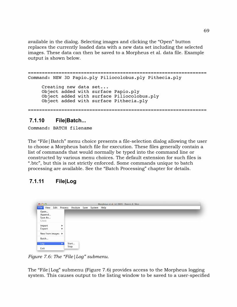
69
available in the dialog. Selecting images and clicking the “Open” button replaces the currently loaded data with a new data set including the selected images. These data can then be saved to a Morpheus et al. data file. Example output is shown below.
================================================================Command: NEW 3D Papio.ply Piliocolobus.ply Pithecia.ply
Creating new data set...Object added with surface Papio.plyObject added with surface Piliocolobus.plyObject added with surface Pithecia.ply
================================================================
7.1.10 File|Batch...Command: BATCH filename
The “File|Batch” menu choice presents a file-selection dialog allowing the user to choose a Morpheus batch file for execution. These files generally contain a list of commands that would normally be typed into the command line or constructed by various menu choices. The default extension for such files is “.btc”, but this is not strictly enforced. Some commands unique to batch processing are available. See the “Batch Processing” chapter for details.
7.1.11 File|Log
The “File|Log” submenu (Figure 7.6) provides access to the Morpheus logging system. This causes output to the listing window to be saved to a user-specified
Figure 7.6: The “File|Log” submenu.
70
ASCII text file.
7.1.12 File|Log|Start...Command: LOG START filename
The “File|Log|Start...” menu choice presents a file-save dialog that allows the user to specify the file to which subsequent listing-window output will be saved. A reasonable extension for such files is .log, but this is not strictly enforced. Example output is shown below.
================================================================Command: LOG START mylog.log
START logging to /Users/myaccount/data/mylog.log
================================================================
7.1.13 File|Log|StopCommand: LOG STOP
The “File|Log|Stop” menu choice forces any buffered output to be written to the currently open log file and closes that file. Example output is shown below.
================================================================Command: LOG STOP
STOP logging to /Users/myaccount/data/mylog.log
================================================================
7.1.14 File|ExitThe “File|Exit” choice terminates the program. This is the only method of termination that will save the current configuration data to the morpheus configuration file. That is, exiting the program via the “Close Window” frame control or by keyboard shortcut does not save the configuration information.
7.2 View
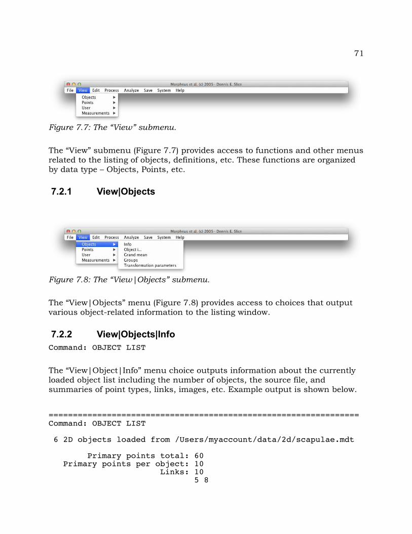
71
The “View” submenu (Figure 7.7) provides access to functions and other menus related to the listing of objects, definitions, etc. These functions are organized by data type – Objects, Points, etc.
7.2.1 View|Objects
The “View|Objects” menu (Figure 7.8) provides access to choices that output various object-related information to the listing window.
7.2.2 View|Objects|InfoCommand: OBJECT LIST
The “View|Object|Info” menu choice outputs information about the currently loaded object list including the number of objects, the source file, and summaries of point types, links, images, etc. Example output is shown below.
================================================================Command: OBJECT LIST
6 2D objects loaded from /Users/myaccount/data/2d/scapulae.mdt
Primary points total: 60 Primary points per object: 10 Links: 10 5 8
Figure 7.7: The “View” submenu.
Figure 7.8: The “View|Objects” submenu.
72
8 10 10 9 9 5 4 1 1 5 5 2 2 6 6 3 3 7 Images total: 6 Images per object: 1
*** Contact author to request additional output ***
================================================================
7.2.3 View|Objects|Object i...Command: OBJECT LIST *Command: OBJECT LIST i
The “View|Objects|Object i...” menu choice opens a dialog with an editable skeleton of the command. The default form, OBJECT LIST *, outputs a summary of the data for all objects to the screen. The more specific form, OBJECTS LIST i, outputs more detailed information about the specified object. Example output for both is shown below. An ellipsis (“...”) indicates text deleted to save space.
================================================================Command: OBJECT LIST *
Obj1: 174722 User vars: 0 Primary points: 10 Secondary points: 0
...
Obj6: 220326 User vars: 0 Primary points: 10 Secondary points: 0
*** Contact author to request additional output ***
================================================================Command: OBJECT LIST 4
73
Obj4: 176228 Dim: 2 Points: 10 Primary points: 10 Secondary points: 0 1. P "" 173.933000 45.933000 2. P "" 9.947000 71.095000 3. P "" 165.887000 121.855000 4. P "" 167.204000 53.979000 5. P "" 89.965000 38.912000 6. P "" 60.562000 105.471000 7. P "" 181.101000 98.596000 8. P "" 200.996000 108.251000 9. P "" 204.506000 92.013000 10. P "" 221.183000 100.059000 _____________________ P=Primary S=Secondary
*** Contact author to request additional output ***
================================================================
7.2.4 View|Objects|GroupsCommand: OBJECT LIST GROUPS
The “View|Object|Groups” command outputs a summary of the current grouping of the objects in the object list. An example is shown below.
================================================================Command: OBJECT LIST GROUPS
6 objects in 2 groups grouped by count...
1) Gorilla - 174722, 174723, 176225 2) Pan - 176228, 220065, 220326
================================================================
7.2.5 View|Objects|List|Transformation parametersCommand: LIST OBJECT TRANSFORMS
The “View|Objects|Transformation parameters” menu choice outputs the current translation, scale, and rotation parameters that have been applied to the coordinate data of each object in the list. Example output after a generalized Procrustes superimposition is shown below. An ellipsis (“...”) indicates text deleted here to save space.
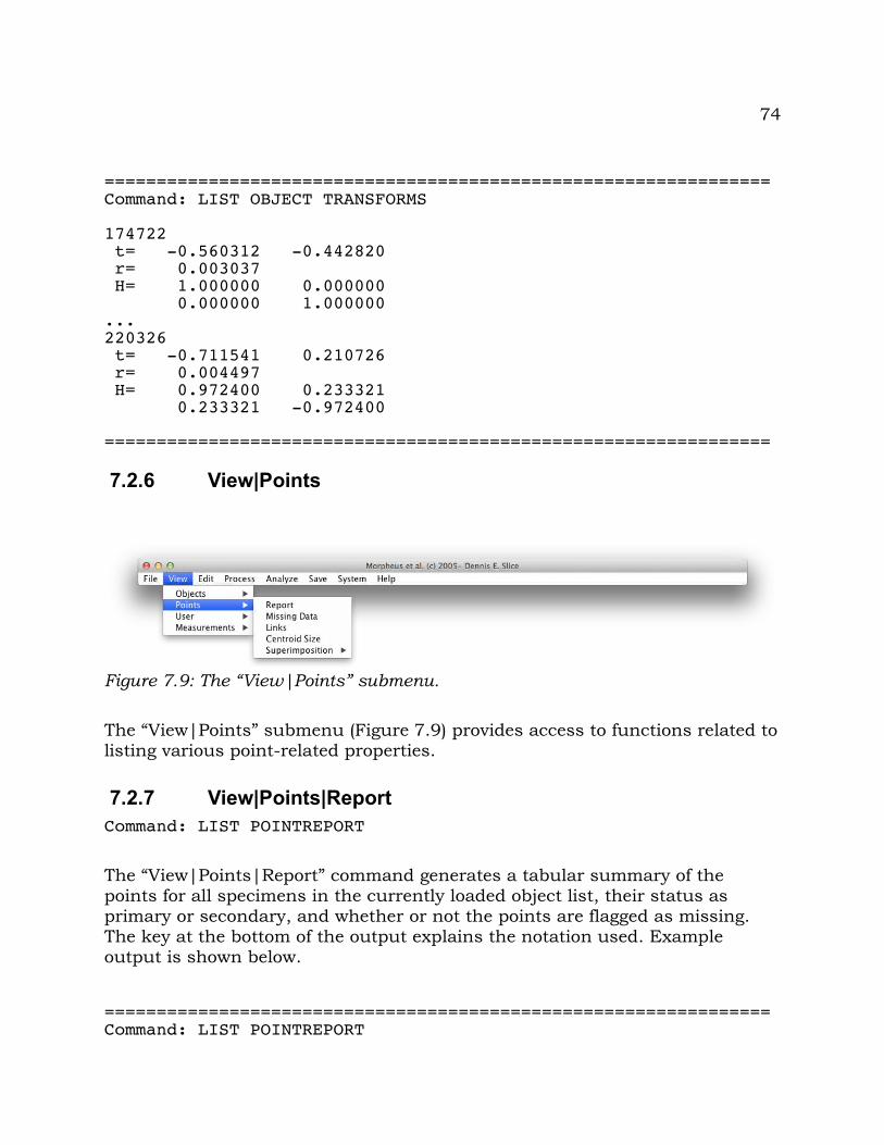
74
================================================================Command: LIST OBJECT TRANSFORMS
174722 t= -0.560312 -0.442820 r= 0.003037 H= 1.000000 0.000000 0.000000 1.000000 ...220326 t= -0.711541 0.210726 r= 0.004497 H= 0.972400 0.233321 0.233321 -0.972400
================================================================
7.2.6 View|Points
The “View|Points” submenu (Figure 7.9) provides access to functions related to listing various point-related properties.
7.2.7 View|Points|ReportCommand: LIST POINTREPORT
The “View|Points|Report” command generates a tabular summary of the points for all specimens in the currently loaded object list, their status as primary or secondary, and whether or not the points are flagged as missing. The key at the bottom of the output explains the notation used. Example output is shown below.
================================================================Command: LIST POINTREPORT
Figure 7.9: The “View|Points” submenu.
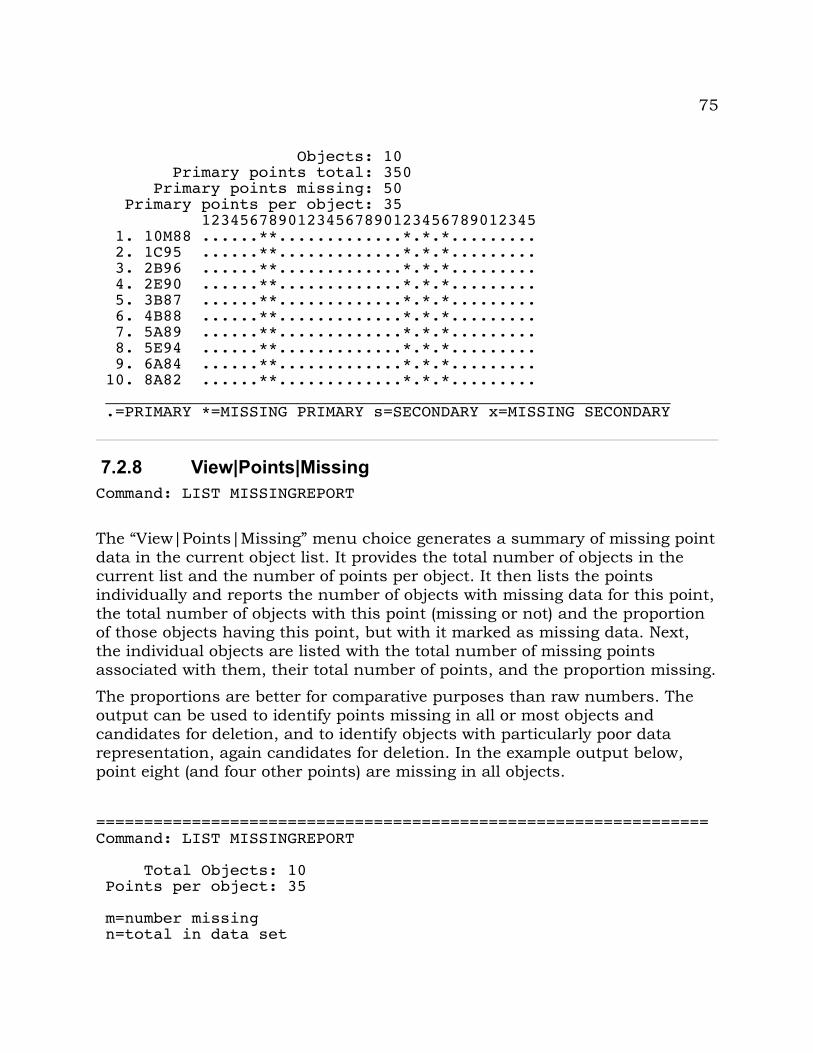
75
Objects: 10 Primary points total: 350 Primary points missing: 50 Primary points per object: 35 12345678901234567890123456789012345 1. 10M88 ......**.............*.*.*......... 2. 1C95 ......**.............*.*.*......... 3. 2B96 ......**.............*.*.*......... 4. 2E90 ......**.............*.*.*......... 5. 3B87 ......**.............*.*.*......... 6. 4B88 ......**.............*.*.*......... 7. 5A89 ......**.............*.*.*......... 8. 5E94 ......**.............*.*.*......... 9. 6A84 ......**.............*.*.*......... 10. 8A82 ......**.............*.*.*......... ___________________________________________________________ .=PRIMARY *=MISSING PRIMARY s=SECONDARY x=MISSING SECONDARY
7.2.8 View|Points|MissingCommand: LIST MISSINGREPORT
The “View|Points|Missing” menu choice generates a summary of missing point data in the current object list. It provides the total number of objects in the current list and the number of points per object. It then lists the points individually and reports the number of objects with missing data for this point, the total number of objects with this point (missing or not) and the proportion of those objects having this point, but with it marked as missing data. Next, the individual objects are listed with the total number of missing points associated with them, their total number of points, and the proportion missing.
The proportions are better for comparative purposes than raw numbers. The output can be used to identify points missing in all or most objects and candidates for deletion, and to identify objects with particularly poor data representation, again candidates for deletion. In the example output below, point eight (and four other points) are missing in all objects.
================================================================Command: LIST MISSINGREPORT
Total Objects: 10 Points per object: 35
m=number missing n=total in data set
76
pro=m/n
Points: # m n pro 1 0 10 0.00
... 8 10 10 1.00 9 0 10 0.00
... 35 0 10 0.00 Objects: # m n pro 1 5 35 0.14
... 10 5 35 0.14
7.2.9 View|Points|LinksThe “View|Points|Links” menu choice generates and displays a list of the current link definitions. Sample output is shown below.================================================================Command: LINK LIST
Links...1. 5 82. 8 103. 10 94. 9 55. 4 16. 1 57. 5 28. 2 69. 6 310. 3 7
================================================================
7.2.10 View|Points|Centroid SizeCommand: LIST CENTROIDSIZE
The “View|Points|Centroid Size” menu choice generates a list of the centroid sizes of the current objects. These values were calculated when the data were loaded, and any object with missing data for any of the primary points will have its CS reported as *MISSING*. Example output is shown below.
================================================================Command: LIST CENTROIDSIZE
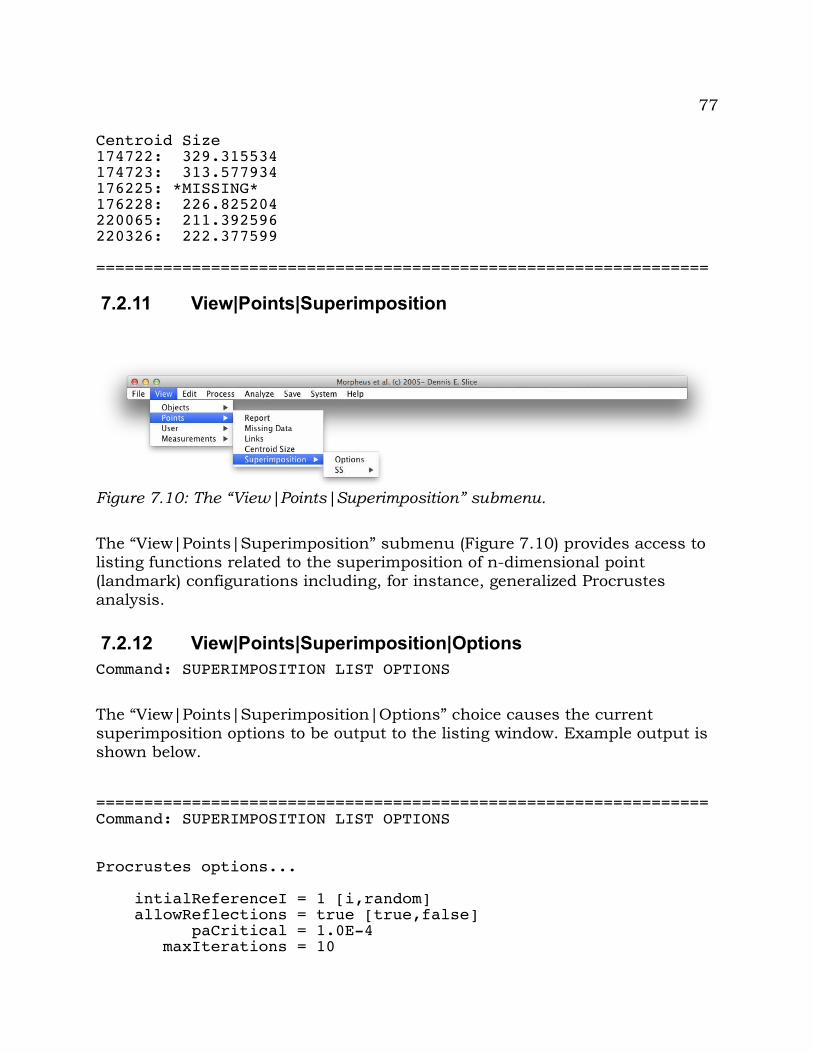
77
Centroid Size174722: 329.315534174723: 313.577934176225: *MISSING*176228: 226.825204220065: 211.392596220326: 222.377599
================================================================
7.2.11 View|Points|Superimposition
The “View|Points|Superimposition” submenu (Figure 7.10) provides access to listing functions related to the superimposition of n-dimensional point (landmark) configurations including, for instance, generalized Procrustes analysis.
7.2.12 View|Points|Superimposition|OptionsCommand: SUPERIMPOSITION LIST OPTIONS
The “View|Points|Superimposition|Options” choice causes the current superimposition options to be output to the listing window. Example output is shown below.
================================================================Command: SUPERIMPOSITION LIST OPTIONS
Procrustes options...
intialReferenceI = 1 [i,random] allowReflections = true [true,false] paCritical = 1.0E-4 maxIterations = 10
Figure 7.10: The “View|Points|Superimposition” submenu.
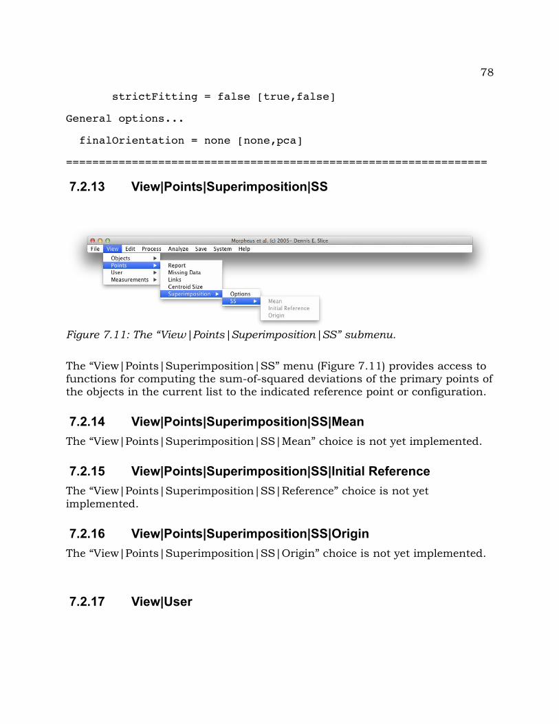
78
strictFitting = false [true,false]
General options...
finalOrientation = none [none,pca]
================================================================
7.2.13 View|Points|Superimposition|SS
The “View|Points|Superimposition|SS” menu (Figure 7.11) provides access to functions for computing the sum-of-squared deviations of the primary points of the objects in the current list to the indicated reference point or configuration.
7.2.14 View|Points|Superimposition|SS|MeanThe “View|Points|Superimposition|SS|Mean” choice is not yet implemented.
7.2.15 View|Points|Superimposition|SS|Initial ReferenceThe “View|Points|Superimposition|SS|Reference” choice is not yet implemented.
7.2.16 View|Points|Superimposition|SS|OriginThe “View|Points|Superimposition|SS|Origin” choice is not yet implemented.
7.2.17 View|User
Figure 7.11: The “View|Points|Superimposition|SS” submenu.
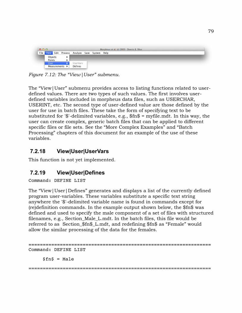
79
The “View|User” submenu provides access to listing functions related to user-defined values. There are two types of such values. The first involves user-defined variables included in morpheus data files, such as USERCHAR, USERINT, etc. The second type of user-defined value are those defined by the user for use in batch files. These take the form of specifying text to be substituted for '$'-delimited variables, e.g., $fn$ = myfile.mdt. In this way, the user can create complex, generic batch files that can be applied to different specific files or file sets. See the “More Complex Examples” and “Batch Processing” chapters of this document for an example of the use of these variables.
7.2.18 View|User|UserVarsThis function is not yet implemented.
7.2.19 View|User|DefinesCommand: DEFINE LIST
The “View|User|Defines” generates and displays a list of the currently defined program user-variables. These variables substitute a specific text string anywhere the '$'-delimited variable name is found in commands except for (re)definition commands. In the example output shown below, the $fn$ was defined and used to specify the male component of a set of files with structured filenames, e.g., Section_Male_L.mdt. In the batch files, this file would be referred to as Section_$fn$_L.mdt, and redefining $fn$ as “Female” would allow the similar processing of the data for the females.
================================================================Command: DEFINE LIST
$fn$ = Male
================================================================
Figure 7.12: The “View|User” submenu.
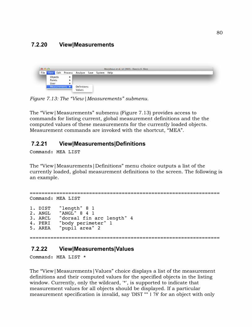
80
7.2.20 View|Measurements
The “View|Measurements” submenu (Figure 7.13) provides access to commands for listing current, global measurement definitions and the the computed values of these measurements for the currently loaded objects. Measurement commands are invoked with the shortcut, “MEA”.
7.2.21 View|Measurements|DefinitionsCommand: MEA LIST
The “View|Measurements|Definitions” menu choice outputs a list of the currently loaded, global measurement definitions to the screen. The following is an example.
================================================================Command: MEA LIST
1. DIST "length" 8 12. ANGL "ANGL" 8 4 13. ARCL "dorsal fin arc length" 44. PERI "body perimeter" 15. AREA "pupil area" 2
================================================================
7.2.22 View|Measurements|ValuesCommand: MEA LIST *
The “View|Measurements|Values” choice displays a list of the measurement definitions and their computed values for the specified objects in the listing window. Currently, only the wildcard, '*', is supported to indicate that measurement values for all objects should be displayed. If a particular measurement specification is invalid, say 'DIST "" 1 78' for an object with only
Figure 7.13: The “View|Measurements” submenu.
81
twelve primary points, the value is reported as “NaN” - “Not a Number”. If the measurement is defined, but necessary data for its computation is marked as missing, the value is reported as “*MISSING*”.
An example is shown below. The ellipsis (“...”) indicates data deleted to save space. After the measurement definitions, the results begin with a row number indicating the object being measured and its label. Measurements follow on the same line.
================================================================Command: MEA LIST *
1. AREA "AREA" 12. AREA "AREA" 23. AREA "AREA" 34. TRIAREA "TRIAREA" 3 1 25. TRIAREA "TRIAREA" 4 1 26. TRIAREA "TRIAREA" 4 1 37. TRIAREA "TRIAREA" 6 1 28. TRIAREA "TRIAREA" 7 1 29. TRIAREA "TRIAREA" 9 1 210. DIST "DIST" 2 111. DIST "DIST" 3 012. DIST "DIST" 3 113. DIST "DIST" 3 214. DIST "DIST" 9 115. TRIAREA "TRIAREA" 3 1 216. ARCL "ARCL" 117. PERI "PERI" 118. ARCL "ARCL" 219. PERI "PERI" 220. ARCL "ARCL" 321. PERI "PERI" 3
1. "O1" 3.141433 3.455850 NaN 0.500000 ...
2. "w/Missing" NaN 3.455850 NaN *MISSING* 0.000000...
ListAll Under construction.
================================================================
7.3 Edit
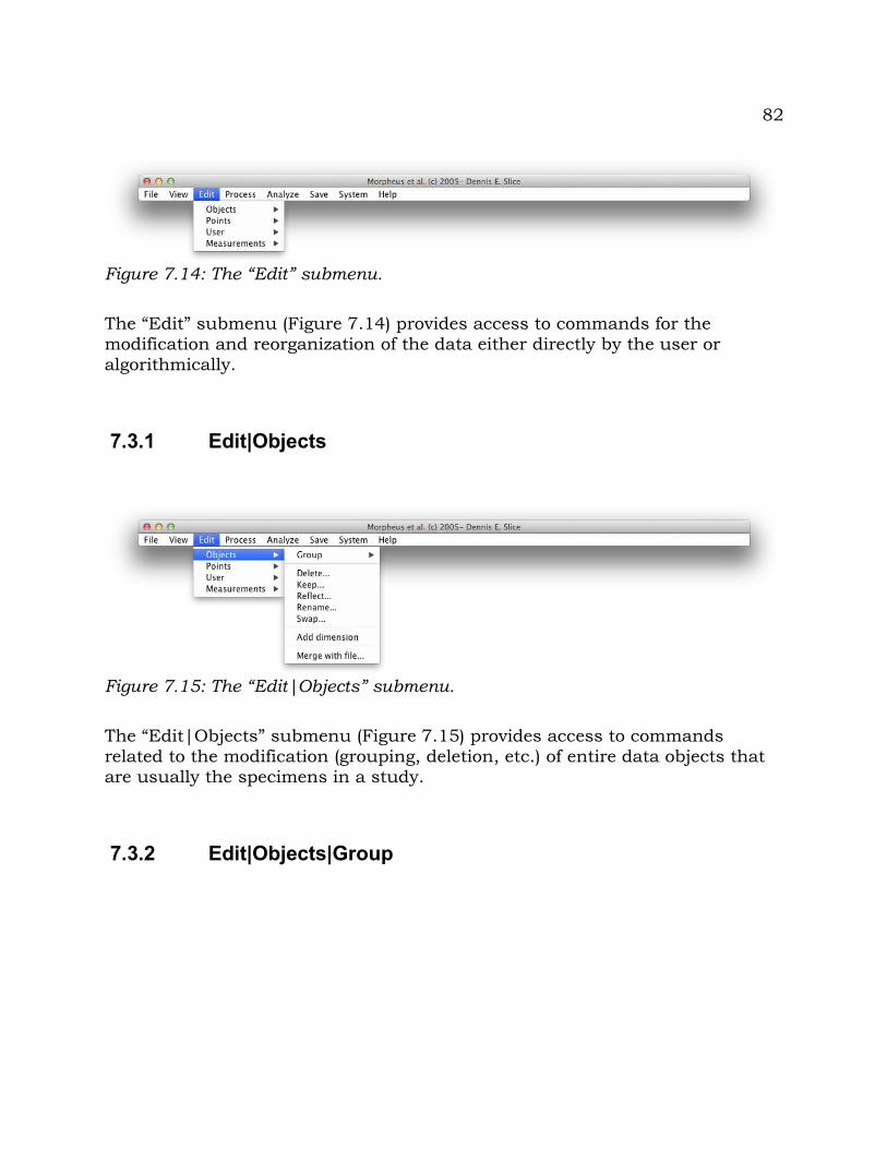
82
The “Edit” submenu (Figure 7.14) provides access to commands for the modification and reorganization of the data either directly by the user or algorithmically.
7.3.1 Edit|Objects
The “Edit|Objects” submenu (Figure 7.15) provides access to commands related to the modification (grouping, deletion, etc.) of entire data objects that are usually the specimens in a study.
7.3.2 Edit|Objects|Group
Figure 7.14: The “Edit” submenu.
Figure 7.15: The “Edit|Objects” submenu.
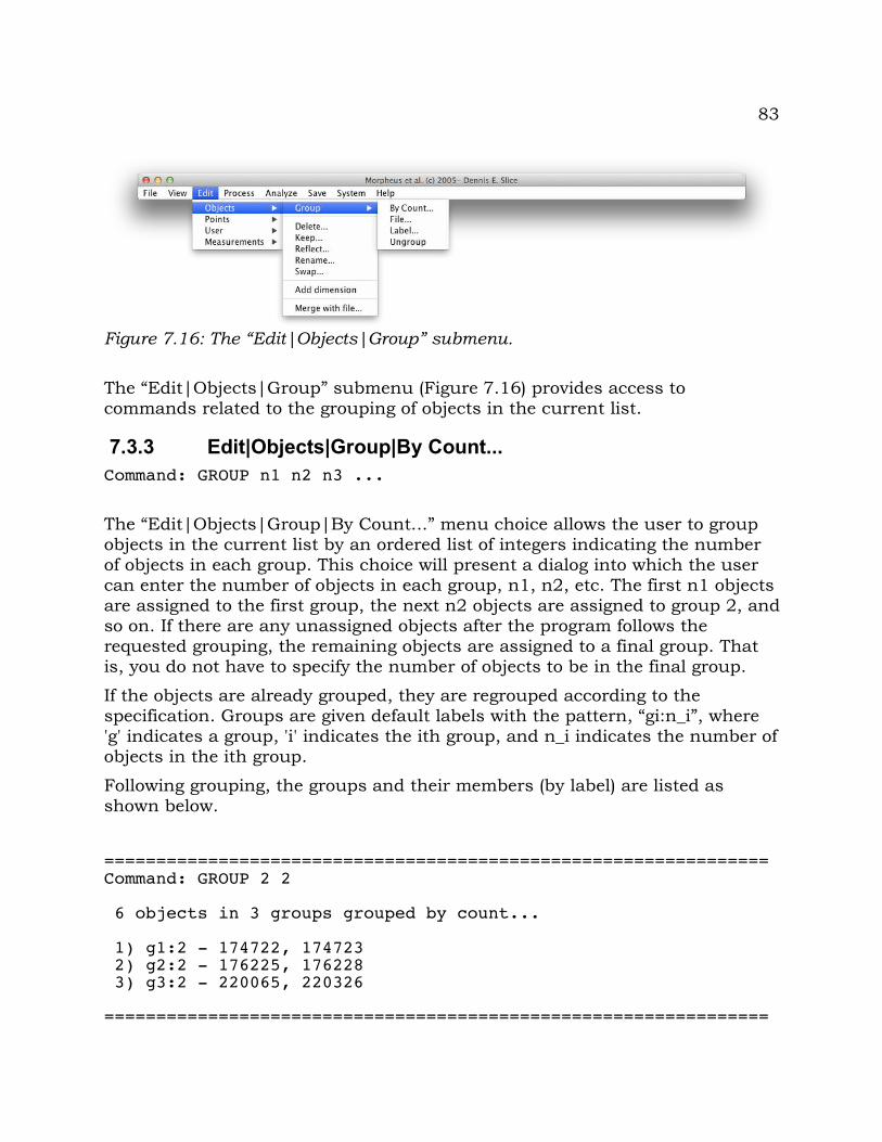
83
The “Edit|Objects|Group” submenu (Figure 7.16) provides access to commands related to the grouping of objects in the current list.
7.3.3 Edit|Objects|Group|By Count...Command: GROUP n1 n2 n3 ...
The “Edit|Objects|Group|By Count...” menu choice allows the user to group objects in the current list by an ordered list of integers indicating the number of objects in each group. This choice will present a dialog into which the user can enter the number of objects in each group, n1, n2, etc. The first n1 objects are assigned to the first group, the next n2 objects are assigned to group 2, and so on. If there are any unassigned objects after the program follows the requested grouping, the remaining objects are assigned to a final group. That is, you do not have to specify the number of objects to be in the final group.
If the objects are already grouped, they are regrouped according to the specification. Groups are given default labels with the pattern, “gi:n_i”, where 'g' indicates a group, 'i' indicates the ith group, and n_i indicates the number of objects in the ith group.
Following grouping, the groups and their members (by label) are listed as shown below.
================================================================Command: GROUP 2 2
6 objects in 3 groups grouped by count...
1) g1:2 - 174722, 174723 2) g2:2 - 176225, 176228 3) g3:2 - 220065, 220326
================================================================
Figure 7.16: The “Edit|Objects|Group” submenu.
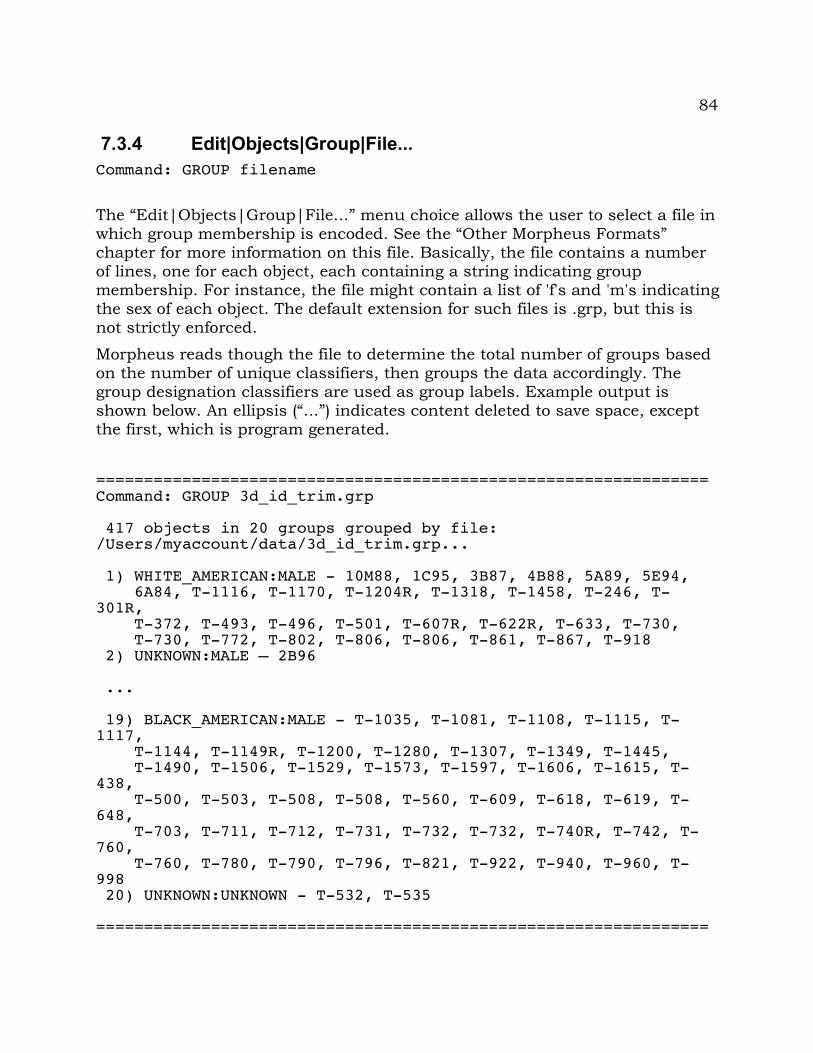
84
7.3.4 Edit|Objects|Group|File...Command: GROUP filename
The “Edit|Objects|Group|File...” menu choice allows the user to select a file in which group membership is encoded. See the “Other Morpheus Formats” chapter for more information on this file. Basically, the file contains a number of lines, one for each object, each containing a string indicating group membership. For instance, the file might contain a list of 'f's and 'm's indicating the sex of each object. The default extension for such files is .grp, but this is not strictly enforced.
Morpheus reads though the file to determine the total number of groups based on the number of unique classifiers, then groups the data accordingly. The group designation classifiers are used as group labels. Example output is shown below. An ellipsis (“...”) indicates content deleted to save space, except the first, which is program generated.
================================================================Command: GROUP 3d_id_trim.grp
417 objects in 20 groups grouped by file: /Users/myaccount/data/3d_id_trim.grp...
1) WHITE_AMERICAN:MALE - 10M88, 1C95, 3B87, 4B88, 5A89, 5E94, 6A84, T-1116, T-1170, T-1204R, T-1318, T-1458, T-246, T-301R, T-372, T-493, T-496, T-501, T-607R, T-622R, T-633, T-730, T-730, T-772, T-802, T-806, T-806, T-861, T-867, T-918 2) UNKNOWN:MALE – 2B96
...
19) BLACK_AMERICAN:MALE - T-1035, T-1081, T-1108, T-1115, T-1117, T-1144, T-1149R, T-1200, T-1280, T-1307, T-1349, T-1445, T-1490, T-1506, T-1529, T-1573, T-1597, T-1606, T-1615, T-438, T-500, T-503, T-508, T-508, T-560, T-609, T-618, T-619, T-648, T-703, T-711, T-712, T-731, T-732, T-732, T-740R, T-742, T-760, T-760, T-780, T-790, T-796, T-821, T-922, T-940, T-960, T-998 20) UNKNOWN:UNKNOWN - T-532, T-535
================================================================
85
7.3.5 Edit|Objects|Group|Label...Command: LABEL GROUPS label_1 label_2 ...
The “Edit|Objects|Group|Label” menu choice allows the user to rename groups. The user is presented with a dialog box into which they may type an ordered series of strings that will be used for group labels. While the use of spaces in labels is discouraged, it is supported through the use of quotation marks around the space-containing label. Labels for all groups are not required, and groups can be skipped over for relabelling by using '*', as shown in the example below.
================================================================Command: LABEL GROUPS Gorilla Chimp
6 objects in 2 groups grouped by count...
1) Gorilla - 174722, 174723, 176225 2) Chimp - 176228, 220065, 220326
================================================================Command: LABEL GROUPS * Pan
6 objects in 2 groups grouped by count...
1) Gorilla - 174722, 174723, 176225 2) Pan - 176228, 220065, 220326
================================================================
7.3.6 Edit|Objects|Group|UngroupCommand: UNGROUP
The “Edit|Objects|Group|Ungroup” choice removes object grouping. Objects are effectively put into a single group, but a single group has no special designation or labeling. Example output follows.
================================================================Command: UNGROUP
6 objects ungrouped.================================================================
7.3.7 Edit|Objects|Delete...Command: DELETE OBJECT(S) iSeq
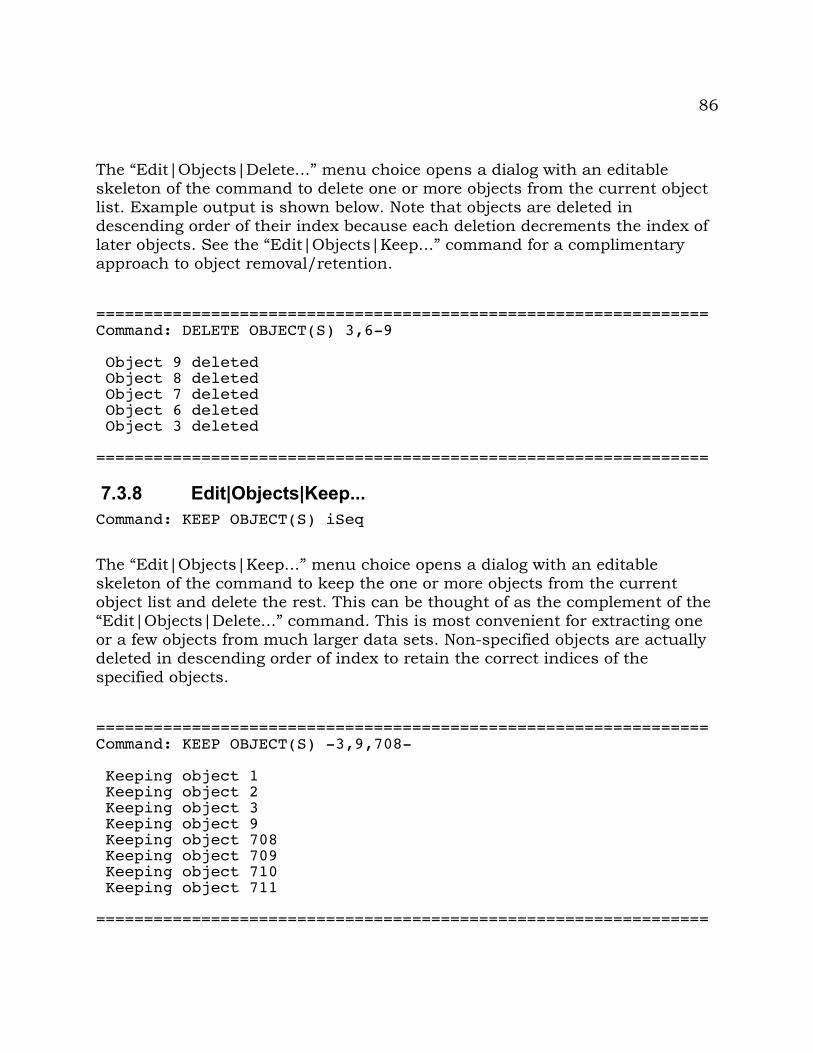
86
The “Edit|Objects|Delete...” menu choice opens a dialog with an editable skeleton of the command to delete one or more objects from the current object list. Example output is shown below. Note that objects are deleted in descending order of their index because each deletion decrements the index of later objects. See the “Edit|Objects|Keep...” command for a complimentary approach to object removal/retention.
================================================================Command: DELETE OBJECT(S) 3,6-9
Object 9 deleted Object 8 deleted Object 7 deleted Object 6 deleted Object 3 deleted
================================================================
7.3.8 Edit|Objects|Keep...Command: KEEP OBJECT(S) iSeq
The “Edit|Objects|Keep...” menu choice opens a dialog with an editable skeleton of the command to keep the one or more objects from the current object list and delete the rest. This can be thought of as the complement of the “Edit|Objects|Delete...” command. This is most convenient for extracting one or a few objects from much larger data sets. Non-specified objects are actually deleted in descending order of index to retain the correct indices of the specified objects.
================================================================Command: KEEP OBJECT(S) -3,9,708-
Keeping object 1 Keeping object 2 Keeping object 3 Keeping object 9 Keeping object 708 Keeping object 709 Keeping object 710 Keeping object 711
================================================================
87
7.3.9 Edit|Objects|Reflect...Command: OBJECT REFLECT iSeq
The “Edit|Obects|Reflect...” menu opens a dialog with a editable skeleton of the command to reflect one or more objects. Reflection is achieved by simply multiplying the x coordinate of data and the first column of the rotation matrix associated with an image or surface by -1.0. Note that at this time, this has the effect of turning surfaces “inside out”.
================================================================Command: OBJECT REFLECT 1,3,5
Reflecting object 1 Reflecting object 3 Reflecting object 5
================================================================
7.3.10 Edit|Objects|Rename...Command: OBJECT RENAME i|LAST new_name
The “Edit|Objects|Rename” menu choice opens a dialog with a editable skeleton of the command to rename either the ith or last object in the current object list. The LAST parameter is supported so as not to require the user to know the exact object count when renaming a newly added object. Example output is shown below.
================================================================Command: OBJECT RENAME 2 second
Label of Obj 2 changed from 174723 to second
================================================================Command: OBJECT RENAME LAST last
Label of Obj 6 changed from 220326 to last
================================================================
7.3.11 Edit|Objects|Swap...Command: SWAP OBJECTS i j
88
The “Edit|Objects|Swap...” menu choice opens a dialog with an editable skeleton of the command to swap the positions of two objects, i and j, in the current object list. Example output is shown below.
================================================================Command: SWAP OBJECTS 4 5
Objects 4 and 5 swapped================================================================
7.3.12 Edit|Objects|Add dimensionCommand: OBJECT ADDDIM
The “Edit|Objects|Add dimension” menu choice adds one dimension (2D->3D, 3D->4D, etc.) to all objects in the current data set. Coordinate values for this dimension are all set to 0.0, and images and surfaces associated with a given object are deleted. This function was develop to be used in combination with the “Edit|Points|Copy...” and “Edit|Points|Adjust...” functions to add a dimension to a data set, duplicate one of the existing points, then push that point out into the added dimension. When done properly for appropriate data, this can be used to combine orthogonal, two-dimensional data sets into a three-dimensional one. Example output is shown below.
================================================================Command: OBJECT ADDDIM
Adding dimension to objects... Processing object 1 Processing object 2 Processing object 3 Processing object 4 Processing object 5 Processing object 6 Dimension added to objects.
================================================================
7.3.13 Edit|Objects|Merge with file...Command: FILEMERGE filename
The “Edit|Objects|Merge with file...” menu choice combines data from objects in a second, compatible file with that of objects in the currently loaded data
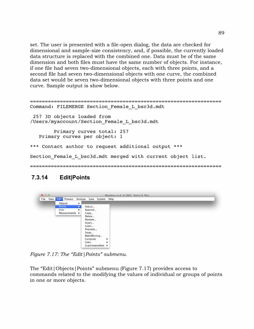
89
set. The user is presented with a file-open dialog, the data are checked for dimensional and sample-size consistency, and, if possible, the currently loaded data structure is replaced with the combined one. Data must be of the same dimension and both files must have the same number of objects. For instance, if one file had seven two-dimensional objects, each with three points, and a second file had seven two-dimensional objects with one curve, the combined data set would be seven two-dimensional objects with three points and one curve. Sample output is show below.
================================================================Command: FILEMERGE Section_Female_L_bsc3d.mdt
257 3D objects loaded from /Users/myaccount/Section_Female_L_bsc3d.mdt
Primary curves total: 257 Primary curves per object: 1
*** Contact author to request additional output ***
Section_Female_L_bsc3d.mdt merged with current object list.
================================================================
7.3.14 Edit|Points
The “Edit|Objects|Points” submenu (Figure 7.17) provides access to commands related to the modifying the values of individual or groups of points in one or more objects.
Figure 7.17: The “Edit|Points” submenu.
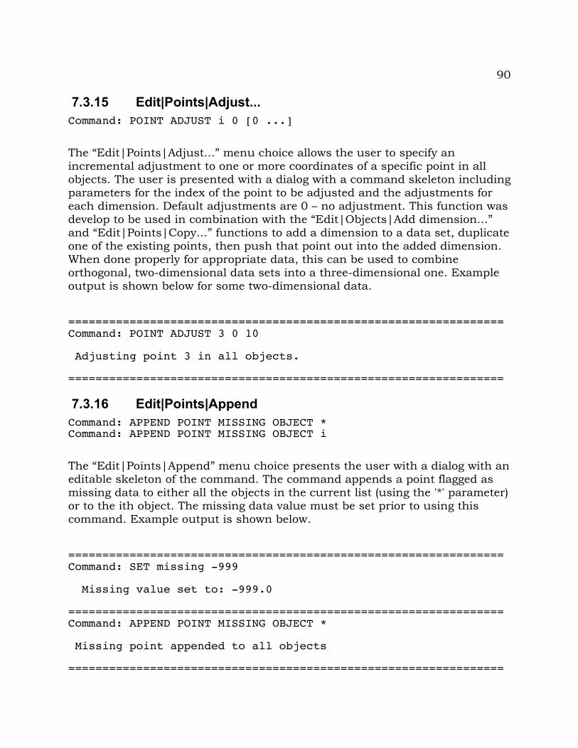
90
7.3.15 Edit|Points|Adjust...Command: POINT ADJUST i 0 [0 ...]
The “Edit|Points|Adjust...” menu choice allows the user to specify an incremental adjustment to one or more coordinates of a specific point in all objects. The user is presented with a dialog with a command skeleton including parameters for the index of the point to be adjusted and the adjustments for each dimension. Default adjustments are 0 – no adjustment. This function was develop to be used in combination with the “Edit|Objects|Add dimension...” and “Edit|Points|Copy...” functions to add a dimension to a data set, duplicate one of the existing points, then push that point out into the added dimension. When done properly for appropriate data, this can be used to combine orthogonal, two-dimensional data sets into a three-dimensional one. Example output is shown below for some two-dimensional data.
================================================================Command: POINT ADJUST 3 0 10
Adjusting point 3 in all objects.
================================================================
7.3.16 Edit|Points|AppendCommand: APPEND POINT MISSING OBJECT *Command: APPEND POINT MISSING OBJECT i
The “Edit|Points|Append” menu choice presents the user with a dialog with an editable skeleton of the command. The command appends a point flagged as missing data to either all the objects in the current list (using the '*' parameter) or to the ith object. The missing data value must be set prior to using this command. Example output is shown below.
================================================================Command: SET missing -999
Missing value set to: -999.0
================================================================Command: APPEND POINT MISSING OBJECT *
Missing point appended to all objects
================================================================
91
Command: APPEND POINT MISSING OBJECT 1
Missing point appended to object 1
================================================================
7.3.17 Edit|Points|Copy...Command: POINT COPY i
The “Edit|Points|Copy...” menu choice allows the user to specify a point to be duplicated in all objects. The new point occupies the index immediately after the duplicated one. This function was develop to be used in combination with the “Edit|Objects|Add dimension...” and “Edit|Points|Adjust...” functions to add a dimension to a data set, duplicate one of the existing points, then push that point out into the added dimension. When done properly for appropriate data, this can be used to combine orthogonal, two-dimensional data sets into a three-dimensional one. Example output is shown below.
================================================================Command: POINT COPY 3
Copying point 3 in all objects.
================================================================
7.3.18 Edit|Points|Delete...Command: DELETE POINT(S) iSeq OBJECT *Command: DELETE POINT(S) iSeq OBJECT iSeq
The “Edit|Points|Delete...” menu choice presents the user with a dialog containing an editable command line. The command deletes one or more points from one or more objects – both specified as iSeq index sequences or the '*' (all objects) parameter. Points are deleted in descending order of the indices. Example output is shown below.
================================================================Command: DELETE POINT(S) 1,5 OBJECT(S) 1-3
Object: 1Deleting point: 5Deleting point: 1
Object: 2Deleting point: 5
92
Deleting point: 1Object: 3
Deleting point: 5Deleting point: 1
================================================================
7.3.19 Edit|Points|Demote...Command: DEMOTE POINT(S) * OBJECT(S) *Command: DEMOTE POINT(S) iSeq OBJECT(S) iSeq
The “Edit|Points|Demote...” menu choice presents the user with a dialog containing an editable command string. The command demotes one or more points in one or more objects as specified by either the '*' parameter (all points or objects) or an iSeq specifying individual or ranges of indices. Demotion means changing the point class from primary (used in point-based computations) to secondary, which are ignored in computations, but carried along with any transformations. Points are demoted in descending order of index for no apparent reason – probably carried over from copy-and-pasting code for deletion. Example output is shown below.
================================================================Command: DEMOTE POINT(S) 2-4 OBJECT(S) *
Object: 1Demoting point: 4Demoting point: 3Demoting point: 2
Object: 2Demoting point: 4Demoting point: 3Demoting point: 2
Object: 3Demoting point: 4Demoting point: 3Demoting point: 2
Object: 4Demoting point: 4Demoting point: 3Demoting point: 2
Object: 5Demoting point: 4Demoting point: 3Demoting point: 2
Object: 6Demoting point: 4Demoting point: 3
93
Demoting point: 2
================================================================
7.3.20 Edit|Points|Insert...Command: INSERT POINT(S) * OBJECT(S) *Command: INSERT POINT(S) iSeq OBJECT(S) iSeq
The “Edit|Points|Insert...” menu choice presents the user with a dialog containing an editable command string. The command inserts one or more data points, marked as missing data, into one or more objects as specified by the iSeq index parameter. The '*' character may be used to specify all points or objects. Example output is shown below.
================================================================Command: INSERT POINT(S) 3 OBJECT(S) 2
Object: 2Inserting point: 3
================================================================Command: INSERT POINT(S) 6 OBJECT(S) *
Object: 1Inserting point: 6
Object: 2Inserting point: 6
Object: 3Inserting point: 6
Object: 4Inserting point: 6
Object: 5Inserting point: 6
Object: 6Inserting point: 6
================================================================
7.3.21 Edit|Points|Label...Command: LABEL POINT i new_label OBJECT *Command: LABEL POINT i new_label OBJECT j
The “Edit|Points|Label...” menu choice presents the user with a dialog containing an editable command string. The command sets the label of the ith point to the specified string for either all objects (when using the '*' parameter)
94
or for just the ith object. Example output is shown below.
================================================================Command: LABEL POINT 1 new_label OBJECT *
Point 1 label set to 'new_label' for all objects
================================================================Command: LABEL POINT 1 new_label_for_object_1 OBJECT 1
Point 1 label set to 'new_label_for_object_1' for object 1
================================================================
7.3.22 Edit|Points|MakeMissing...Command: MAKEMISSING POINT i OBJECT *Command: MAKEMISSING POINT i OBJECT j
The “Edit|Points|MakeMissing...” menu choice presents the user with a dialog containing an editable command string. The command marks the ith point as missing data in either all objects (when the '*' parameter is used) or the jth object only. Example output is shown below.
================================================================Command: SET missing -999
Missing value set to: -999.0
================================================================Command: MAKEMISSING POINT 1 OBJECT *
Point 1 made missing for all objects
================================================================Command: MAKEMISSING POINT 2 OBJECT 1
Point 2 made missing for object 1
================================================================
7.3.23 Edit|Points|Promote...Command: PROMOTE POINT iSeq OBJECT *Command: PROMOTE POINT iSeq OBJECT iSeq
The “Edit|Points|Promote...” menu choice presents the user with a dialog
95
containing an editable command string. The command promotes one or more points in one or more objects as specified by the iSeq or '*' parameter. Promotion means changing the point class from secondary, which is ignored in computations, but carried along with any transformations, to primary, which is used for point-based computations. Promotion of primary points does nothing. Example output is shown below.
================================================================Command: PROMOTE POINT 1 OBJECT *
Point 1 promoted for all objects
================================================================Command: PROMOTE POINT 1 OBJECT 1
Point 1 promoted for object 1
================================================================
7.3.24 Edit|Points|Swap...Command: SWAP POINTS i j OBJECT *Command: SWAP POINTS i j OBJECT k
The “Edit|Points|Swap...” menu choice presents the user with a dialog containing an editable command string. The command swaps the positions of the ith and jth points in either all objects (when using the '*' parameter) or for the kth object only. Example output is shown below.
================================================================Command: SWAP POINTS 1 2 OBJECT *
Points 1 and 2 swapped for all objects
================================================================Command: SWAP POINTS 1 2 OBJECT 3
Points 1 and 2 swapped for object 3
================================================================
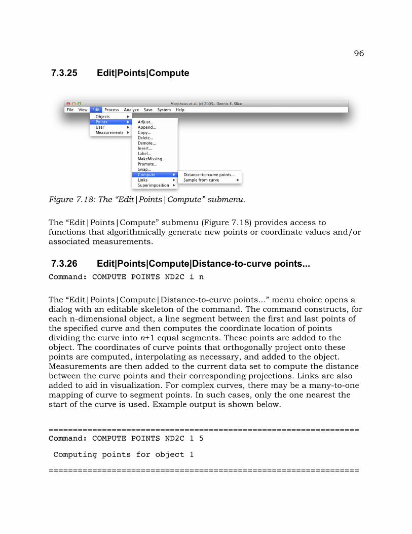
96
7.3.25 Edit|Points|Compute
The “Edit|Points|Compute” submenu (Figure 7.18) provides access to functions that algorithmically generate new points or coordinate values and/or associated measurements.
7.3.26 Edit|Points|Compute|Distance-to-curve points...Command: COMPUTE POINTS ND2C i n
The “Edit|Points|Compute|Distance-to-curve points...” menu choice opens a dialog with an editable skeleton of the command. The command constructs, for each n-dimensional object, a line segment between the first and last points of the specified curve and then computes the coordinate location of points dividing the curve into n+1 equal segments. These points are added to the object. The coordinates of curve points that orthogonally project onto these points are computed, interpolating as necessary, and added to the object. Measurements are then added to the current data set to compute the distance between the curve points and their corresponding projections. Links are also added to aid in visualization. For complex curves, there may be a many-to-one mapping of curve to segment points. In such cases, only the one nearest the start of the curve is used. Example output is shown below.
================================================================Command: COMPUTE POINTS ND2C 1 5
Computing points for object 1
================================================================
Figure 7.18: The “Edit|Points|Compute” submenu.
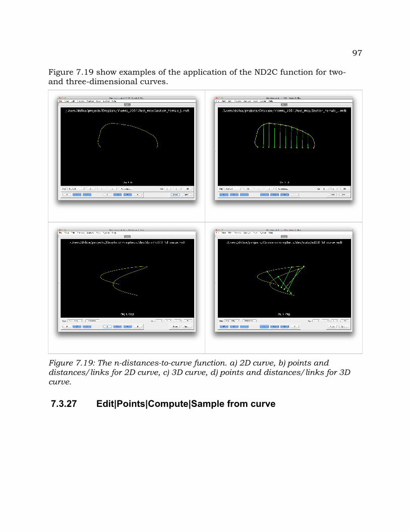
97
Figure 7.19 show examples of the application of the ND2C function for two- and three-dimensional curves.
Figure 7.19: The n-distances-to-curve function. a) 2D curve, b) points and distances/links for 2D curve, c) 3D curve, d) points and distances/links for 3D curve.
7.3.27 Edit|Points|Compute|Sample from curve

98
The “Edit|Points|Sample from curve” submenu (Figure 7.20) provides access to functions related to generating points by sampling curves.
7.3.28 Edit|Points|Sample from curve|Sample...Command: SAMPLE i/label n OPEN/CLOSED
The “Edit|Points|Sample from curve|Sample...” choice opens a dialog with which the user can specify the curve to be sampled (either by index or label), the number of points to sample, and whether or not the curve is open or closed. Open curves are evenly sampled between the first and last points. For closed curves, sampling is evenly spaced around the curve perimeter including the distance between the last and first point. Point labels are autogenerated to indicate the source curve and point index. Sampled points are retained in a temporary data structure until they are explicitly merged with the data of the current object list. Example output for the sampling of an object list containing a single object is shown below.
================================================================Command: SAMPLE 1 5 OPEN
CurveID(int): 1 CurveType: OPEN NPts: 5 PtLabel: C1_Pi
Processing...
Obj 1: Sampling curve 1
================================================================
Figure 7.20: The “Edit|Points|Compute|Sample from curve” submenu.
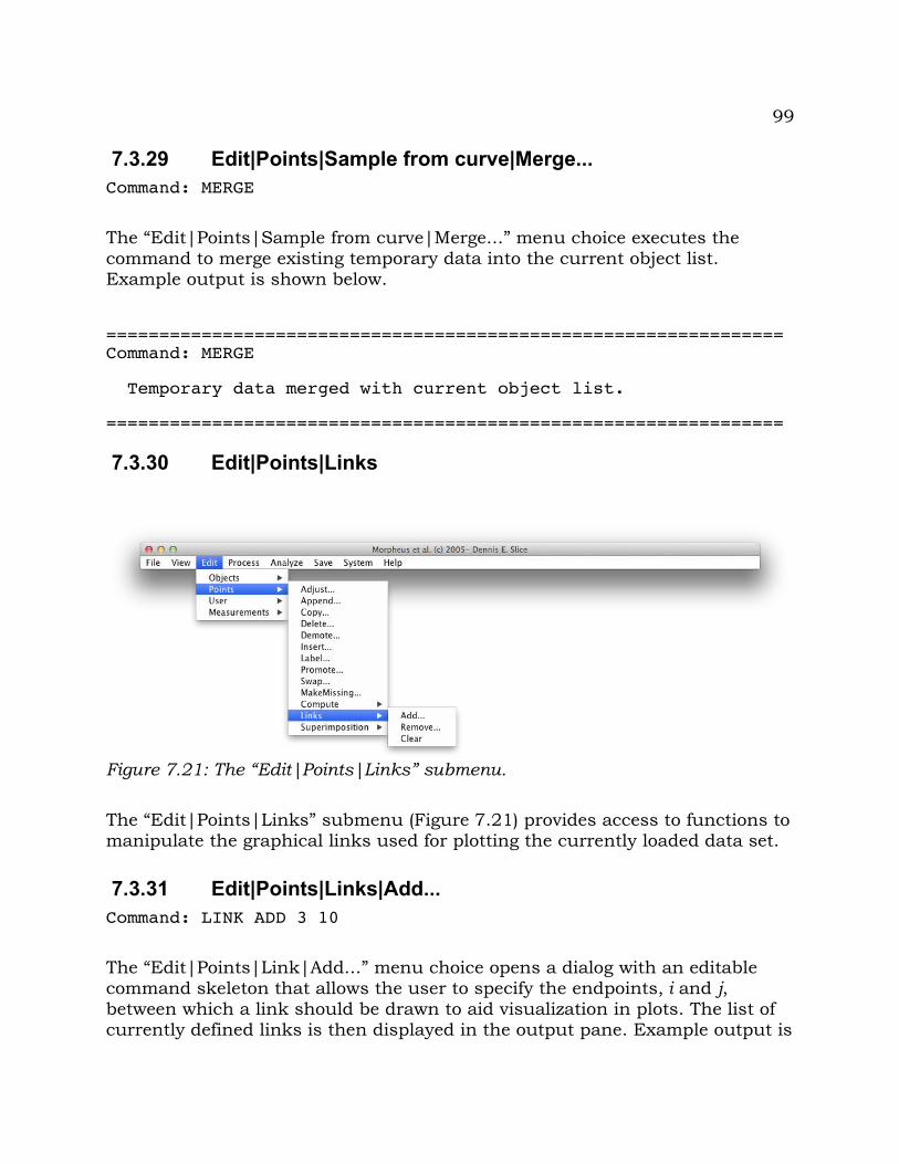
99
7.3.29 Edit|Points|Sample from curve|Merge...Command: MERGE
The “Edit|Points|Sample from curve|Merge...” menu choice executes the command to merge existing temporary data into the current object list. Example output is shown below.
================================================================Command: MERGE
Temporary data merged with current object list.
================================================================
7.3.30 Edit|Points|Links
The “Edit|Points|Links” submenu (Figure 7.21) provides access to functions to manipulate the graphical links used for plotting the currently loaded data set.
7.3.31 Edit|Points|Links|Add...Command: LINK ADD 3 10
The “Edit|Points|Link|Add...” menu choice opens a dialog with an editable command skeleton that allows the user to specify the endpoints, i and j, between which a link should be drawn to aid visualization in plots. The list of currently defined links is then displayed in the output pane. Example output is
Figure 7.21: The “Edit|Points|Links” submenu.
100
shown below.
================================================================Command: LINK ADD 3 10
Adding link...Links...
1. 1 22. 3 43. 5 64. 7 85. 9 106. 3 10
================================================================
7.3.32 Edit|Points|Links|Remove...Command: LINK REMOVE iSeq
The “Edit|Points|Links|Remove...” menu choice first displays a list of currently defined graphical links, then opens a dialog with an editable command line that allows the user to specify one or more links (via the iSeq parameter) to remove from the list. Example output is shown below.
================================================================Command: LINK LIST
Links...1. 1 22. 3 43. 5 64. 7 85. 9 106. 3 10
================================================================Command: LINK REMOVE 3-5
Removing link 5Removing link 4Removing link 3Links...
1. 1 22. 3 43. 3 10
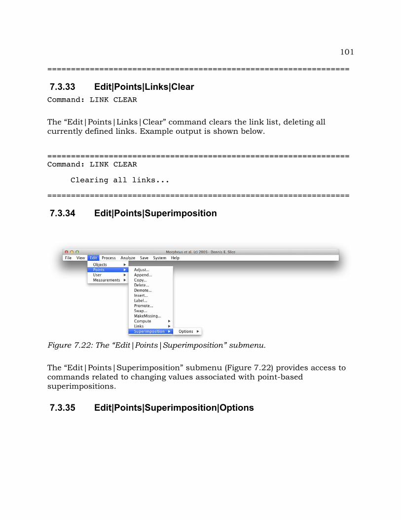
101
================================================================
7.3.33 Edit|Points|Links|ClearCommand: LINK CLEAR
The “Edit|Points|Links|Clear” command clears the link list, deleting all currently defined links. Example output is shown below.
================================================================Command: LINK CLEAR
Clearing all links...
================================================================
7.3.34 Edit|Points|Superimposition
The “Edit|Points|Superimposition” submenu (Figure 7.22) provides access to commands related to changing values associated with point-based superimpositions.
7.3.35 Edit|Points|Superimposition|Options
Figure 7.22: The “Edit|Points|Superimposition” submenu.
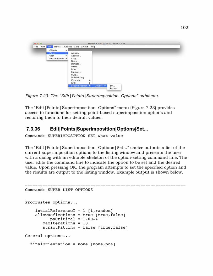
102
The “Edit|Points|Superimposition|Options” menu (Figure 7.23) provides access to functions for setting point-based superimposition options and restoring them to their default values.
7.3.36 Edit|Points|Superimposition|Options|Set...Command: SUPERIMPOSITION SET what value
The “Edit|Points|Superimposition|Options|Set...” choice outputs a list of the current superimposition options to the listing window and presents the user with a dialog with an editable skeleton of the option-setting command line. The user edits the command line to indicate the option to be set and the desired value. Upon pressing OK, the program attempts to set the specified option and the results are output to the listing window. Example output is shown below.
================================================================Command: SUPER LIST OPTIONS
Procrustes options...
intialReferenceI = 1 [i,random] allowReflections = true [true,false] paCritical = 1.0E-4 maxIterations = 10 strictFitting = false [true,false]
General options...
finalOrientation = none [none,pca]
Figure 7.23: The “Edit|Points|Superimposition|Options” submenu.
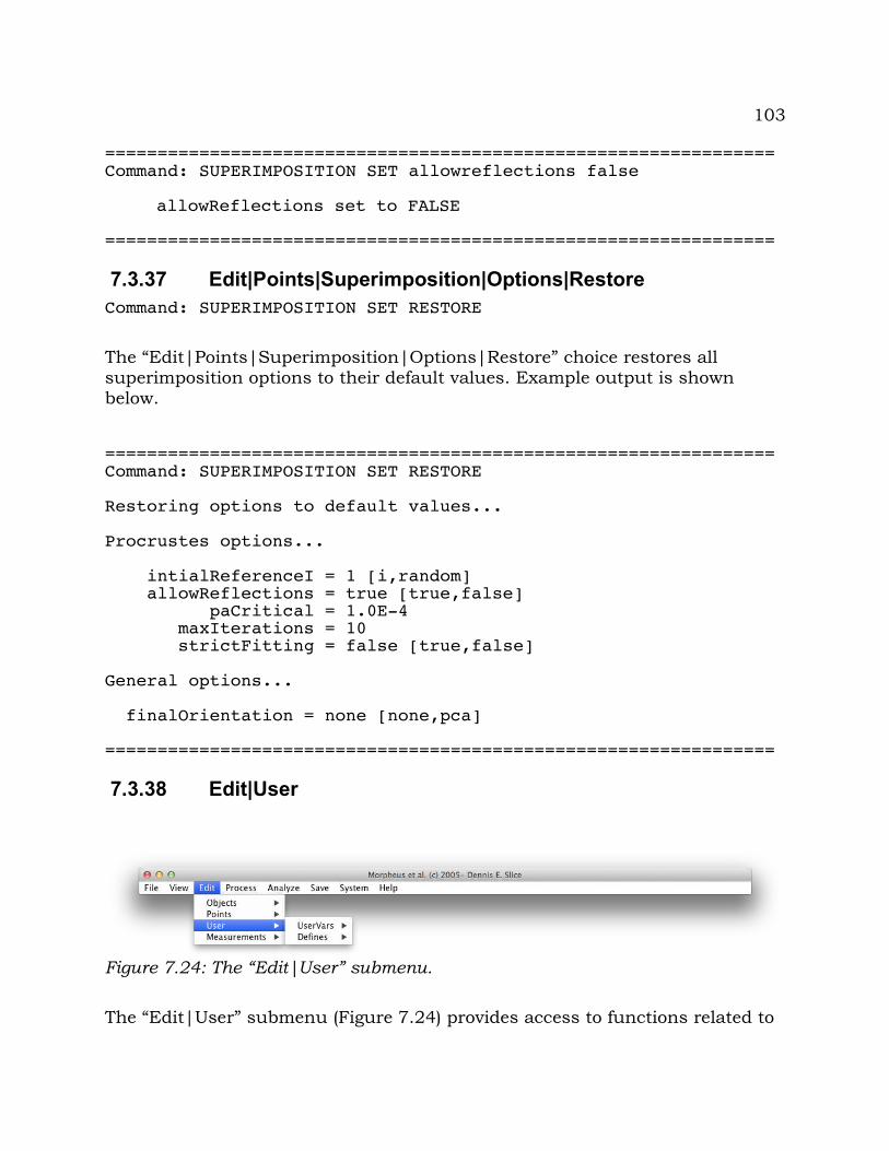
103
================================================================Command: SUPERIMPOSITION SET allowreflections false
allowReflections set to FALSE
================================================================
7.3.37 Edit|Points|Superimposition|Options|RestoreCommand: SUPERIMPOSITION SET RESTORE
The “Edit|Points|Superimposition|Options|Restore” choice restores all superimposition options to their default values. Example output is shown below.
================================================================Command: SUPERIMPOSITION SET RESTORE
Restoring options to default values...
Procrustes options...
intialReferenceI = 1 [i,random] allowReflections = true [true,false] paCritical = 1.0E-4 maxIterations = 10 strictFitting = false [true,false]
General options...
finalOrientation = none [none,pca]
================================================================
7.3.38 Edit|User
The “Edit|User” submenu (Figure 7.24) provides access to functions related to
Figure 7.24: The “Edit|User” submenu.
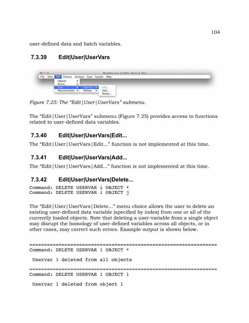
104
user-defined data and batch variables.
7.3.39 Edit|User|UserVars
The “Edit|User|UserVars” submenu (Figure 7.25) provides access to functions related to user-defined data variables.
7.3.40 Edit|User|UserVars|Edit...The “Edit|User|UserVars|Edit...” function is not implemented at this time.
7.3.41 Edit|User|UserVars|Add...The “Edit|User|UserVars|Add...” function is not implemented at this time.
7.3.42 Edit|User|UserVars|Delete...Command: DELETE USERVAR i OBJECT *Command: DELETE USERVAR i OBJECT j
The “Edit|User|UserVars|Delete...” menu choice allows the user to delete an existing user-defined data variable (specified by index) from one or all of the currently loaded objects. Note that deleting a user-variable from a single object may disrupt the homology of user-defined variables across all objects, or in other cases, may correct such errors. Example output is shown below.
================================================================Command: DELETE USERVAR 1 OBJECT *
Uservar 1 deleted from all objects
================================================================Command: DELETE USERVAR 1 OBJECT 1
Uservar 1 deleted from object 1
Figure 7.25: The “Edit|User|UserVars” submenu.
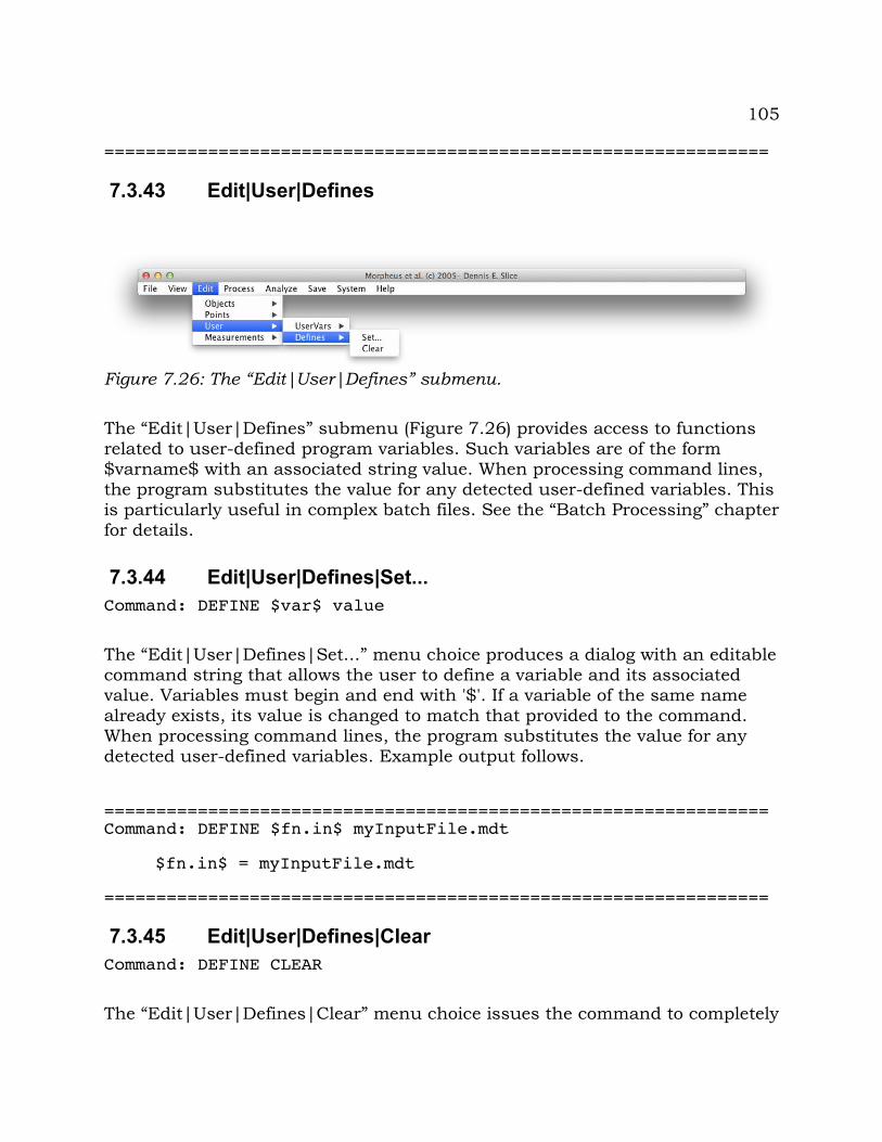
105
================================================================
7.3.43 Edit|User|Defines
The “Edit|User|Defines” submenu (Figure 7.26) provides access to functions related to user-defined program variables. Such variables are of the form $varname$ with an associated string value. When processing command lines, the program substitutes the value for any detected user-defined variables. This is particularly useful in complex batch files. See the “Batch Processing” chapter for details.
7.3.44 Edit|User|Defines|Set...Command: DEFINE $var$ value
The “Edit|User|Defines|Set...” menu choice produces a dialog with an editable command string that allows the user to define a variable and its associated value. Variables must begin and end with '$'. If a variable of the same name already exists, its value is changed to match that provided to the command. When processing command lines, the program substitutes the value for any detected user-defined variables. Example output follows.
================================================================Command: DEFINE $fn.in$ myInputFile.mdt
$fn.in$ = myInputFile.mdt
================================================================
7.3.45 Edit|User|Defines|ClearCommand: DEFINE CLEAR
The “Edit|User|Defines|Clear” menu choice issues the command to completely
Figure 7.26: The “Edit|User|Defines” submenu.
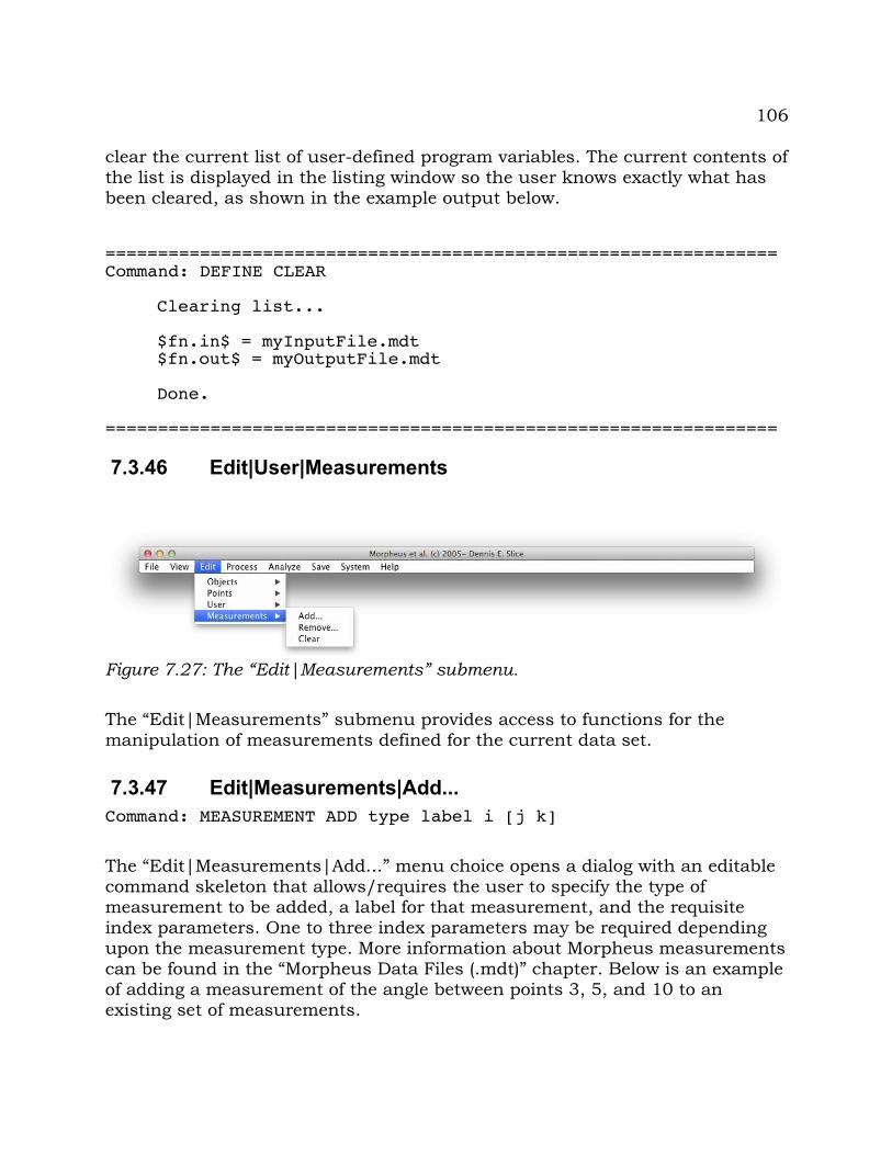
106
clear the current list of user-defined program variables. The current contents of the list is displayed in the listing window so the user knows exactly what has been cleared, as shown in the example output below.
================================================================Command: DEFINE CLEAR
Clearing list...
$fn.in$ = myInputFile.mdt$fn.out$ = myOutputFile.mdt
Done.
================================================================
7.3.46 Edit|User|Measurements
The “Edit|Measurements” submenu provides access to functions for the manipulation of measurements defined for the current data set.
7.3.47 Edit|Measurements|Add...Command: MEASUREMENT ADD type label i [j k]
The “Edit|Measurements|Add...” menu choice opens a dialog with an editable command skeleton that allows/requires the user to specify the type of measurement to be added, a label for that measurement, and the requisite index parameters. One to three index parameters may be required depending upon the measurement type. More information about Morpheus measurements can be found in the “Morpheus Data Files (.mdt)” chapter. Below is an example of adding a measurement of the angle between points 3, 5, and 10 to an existing set of measurements.
Figure 7.27: The “Edit|Measurements” submenu.
107
================================================================Command: MEASUREMENT ADD angle a1 3 5 10
1. DIST "ND2C_1" 2 12. DIST "ND2C_2" 4 33. DIST "ND2C_3" 6 54. DIST "ND2C_4" 8 75. DIST "ND2C_5" 10 96. ANGL "a1" 10 5 3
================================================================
7.3.48 Edit|Measurements|Remove...Command: MEASUREMENT REMOVE iSeq
The “Edit|Measurements|Remove...” menu choice provides for the removal of one or more measurements (specified by an iSeq) defined for the current data set. The program first displays a list of the measurements defined for the current data set. The user is then presented with a dialog with an editable skeleton of the command they can modify to specify which measurements are to be removed from the list. Measurements are removed in descending order of their index. Example output is shown below.
================================================================Command: MEA LIST
1. DIST "ND2C_1" 2 12. DIST "ND2C_2" 4 33. DIST "ND2C_3" 6 54. DIST "ND2C_4" 8 75. DIST "ND2C_5" 10 96. ANGL "a1" 10 5 3
================================================================Command: MEASUREMENT REMOVE -3
Removing measurement 3Removing measurement 2Removing measurement 1
================================================================
7.3.49 Edit|Measurements|ClearCommand: MEA CLEAR
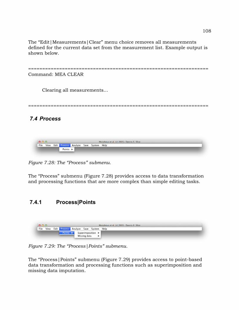
108
The “Edit|Measurements|Clear” menu choice removes all measurements defined for the current data set from the measurement list. Example output is shown below.
================================================================Command: MEA CLEAR
Clearing all measurements...
================================================================
7.4 Process
The “Process” submenu (Figure 7.28) provides access to data transformation and processing functions that are more complex than simple editing tasks.
7.4.1 Process|Points
The “Process|Points” submenu (Figure 7.29) provides access to point-based data transformation and processing functions such as superimposition and missing data imputation.
Figure 7.28: The “Process” submenu.
Figure 7.29: The “Process|Points” submenu.
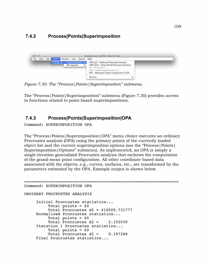
109
7.4.2 Process|Points|Superimposition
The “Process|Points|Superimposition” submenu (Figure 7.30) provides access to functions related to point-based superimpositions.
7.4.3 Process|Points|Superimposition|OPACommand: SUPERIMPOSITION OPA
The “Process|Points|Superimposition|OPA” menu choice executes an ordinary Procrustes analysis (OPA) using the primary points of the currently loaded object list and the current superimposition options (see the “Process|Points|Superimposition|Options” submenu). As implemented, an OPA is simply a single-iteration generalized Procrustes analysis that eschews the computation of the grand-mean point configuration. All other coordinate-based data associated with the objects, e.g., curves, surfaces, etc., are transformed by the parameters estimated by the OPA. Example output is shown below.
================================================================Command: SUPERIMPOSITION OPA
ORDINARY PROCRUSTES ANALYSIS
Initial Procrustes statistics...Total points = 60Total Procrustes d2 = 410009.731777
Normalized Procrustes statistics...Total points = 60Total Procrustes d2 = 2.152039
Iteration 1 Procrustes statistics...Total points = 60Total Procrustes d2 = 0.197288
Final Procrustes statistics...
Figure 7.30: The “Process|Points|Superimposition” submenu.

110
Total points = 60Total Procrustes d2 = 0.197288
================================================================
7.4.4 Process|Points|Superimposition|GPACommand: SUPERIMPOSITION GPA
The “Process|Points|Superimposition|GPA” menu choice executes a generalized Procrustes analysis (GPA) using the primary points of the currently loaded object list and the current superimposition options (see the “Process|Points|Superimposition|Options” submenu). All other coordinate-based data associated with the objects, e.g., curves, surfaces, etc., are transformed by the parameters estimated by the GPA. Example output is shown below.
================================================================Command: SUPERIMPOSITION GPA
GENERALIZED PROCRUSTES ANALYSIS
Initial Procrustes statistics...Total points = 60Total Procrustes d2 = 410009.731777
Normalized Procrustes statistics...Total points = 60Total Procrustes d2 = 2.152039
Iteration 1 Procrustes statistics...Total points = 60Total Procrustes d2 = 0.067980
Iteration 2 Procrustes statistics...Total points = 60Total Procrustes d2 = 0.067935
Final Procrustes statistics...Total points = 60Total Procrustes d2 = 0.067935
================================================================
7.4.5 Process|Points|Superimposition|RFResistant Fitting not yet implemented.
7.4.6 Process|Points|Superimposition|GRFGeneralized Resistant fitting (GRF) not yet implemented.
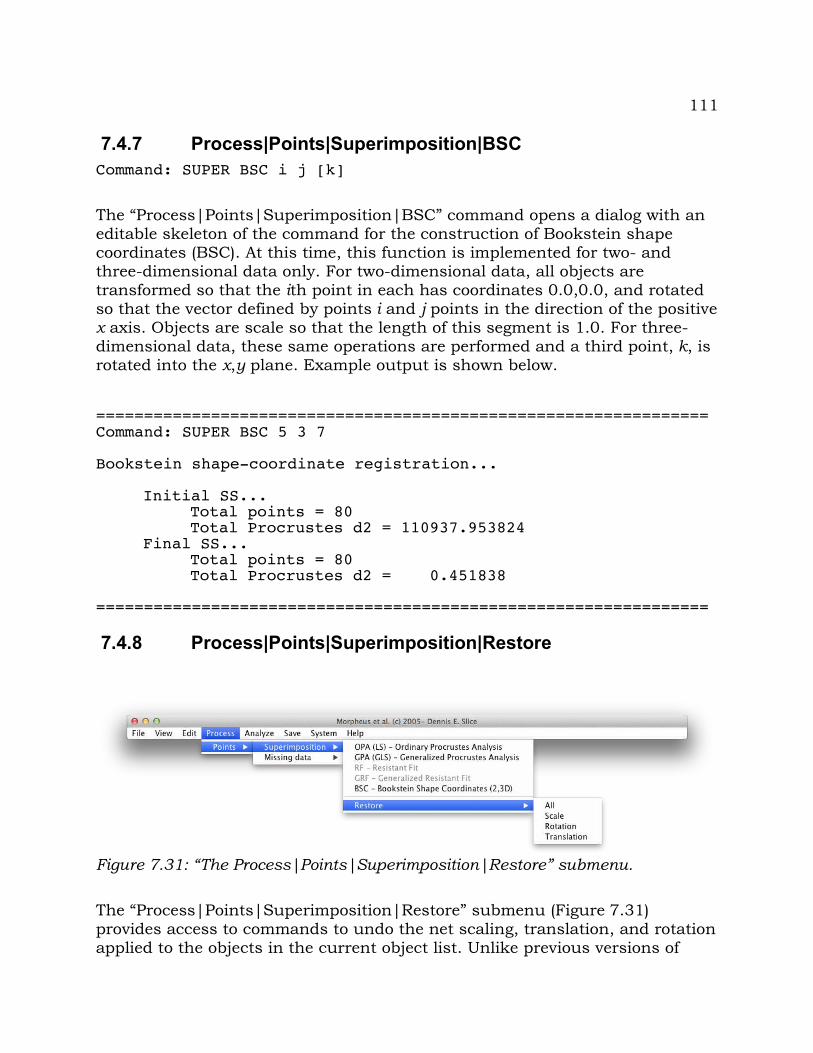
111
7.4.7 Process|Points|Superimposition|BSCCommand: SUPER BSC i j [k]
The “Process|Points|Superimposition|BSC” command opens a dialog with an editable skeleton of the command for the construction of Bookstein shape coordinates (BSC). At this time, this function is implemented for two- and three-dimensional data only. For two-dimensional data, all objects are transformed so that the ith point in each has coordinates 0.0,0.0, and rotated so that the vector defined by points i and j points in the direction of the positive x axis. Objects are scale so that the length of this segment is 1.0. For three-dimensional data, these same operations are performed and a third point, k, is rotated into the x,y plane. Example output is shown below.
================================================================Command: SUPER BSC 5 3 7
Bookstein shape-coordinate registration...
Initial SS...Total points = 80Total Procrustes d2 = 110937.953824
Final SS...Total points = 80Total Procrustes d2 = 0.451838
================================================================
7.4.8 Process|Points|Superimposition|Restore
The “Process|Points|Superimposition|Restore” submenu (Figure 7.31) provides access to commands to undo the net scaling, translation, and rotation applied to the objects in the current object list. Unlike previous versions of
Figure 7.31: “The Process|Points|Superimposition|Restore” submenu.
112
Morpheus et al., these parameters are encoded by tracking identical transformations applied to a set of standard basis vectors generated when the data were loaded. As such, and again unlike earlier versions, the undoing of these transformations is independent of the order of their application. That is, one can restore translation before or after rotation and scaling. The latter have, in previous versions, always been order-independent.
7.4.9 Process|Points|Superimposition|Restore|AllCommand: SUPERIMPOSITION RESTORE ALL
The “Process|Points|Superimposition|Restore|All” menu choice restores the coordinate data (primary and secondary points, curves, etc.) of all objects in the current list to their position, size, and orientation at the time they were read into the program. That is, using this command after a series of transformation operations will restore the coordinate data to their original values. The same can be achieved by the restoration of scale, rotation, and translation terms separately. Example output is shown below.
================================================================Command: SUPERIMPOSITION RESTORE ALL
Restoring... Scale... Rotation... Translation...
================================================================
7.4.10 Process|Points|Superimposition|Restore|ScaleCommand: SUPERIMPOSITION RESTORE SCALE
The “Process|Points|Superimposition|Restore|Scale” menu choice restores the coordinate data (primary and secondary points, curves, etc.) of all objects in the current list to their original size at the time they were read into the program. Complete restoration of the original data can be achieved by the subsequent restoration of rotation and translation. Example output is shown below.================================================================Command: SUPERIMPOSITION RESTORE SCALE
Restoring scale...
================================================================
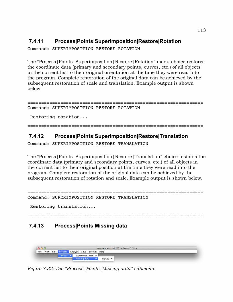
113
7.4.11 Process|Points|Superimposition|Restore|RotationCommand: SUPERIMPOSITION RESTORE ROTATION
The “Process|Points|Superimposition|Restore|Rotation” menu choice restores the coordinate data (primary and secondary points, curves, etc.) of all objects in the current list to their original orientation at the time they were read into the program. Complete restoration of the original data can be achieved by the subsequent restoration of scale and translation. Example output is shown below.
================================================================Command: SUPERIMPOSITION RESTORE ROTATION
Restoring rotation...
================================================================
7.4.12 Process|Points|Superimposition|Restore|TranslationCommand: SUPERIMPOSITION RESTORE TRANSLATION
The “Process|Points|Superimposition|Restore|Translation” choice restores the coordinate data (primary and secondary points, curves, etc.) of all objects in the current list to their original position at the time they were read into the program. Complete restoration of the original data can be achieved by the subsequent restoration of rotation and scale. Example output is shown below.
================================================================Command: SUPERIMPOSITION RESTORE TRANSLATION
Restoring translation...
================================================================
7.4.13 Process|Points|Missing data
Figure 7.32: The “Process|Points|Missing data” submenu.
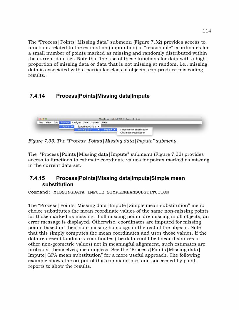
114
The “Process|Points|Missing data” submenu (Figure 7.32) provides access to functions related to the estimation (imputation) of “reasonable” coordinates for a small number of points marked as missing and randomly distributed within the current data set. Note that the use of these functions for data with a high-proportion of missing data or data that is not missing at random, i.e., missing data is associated with a particular class of objects, can produce misleading results.
7.4.14 Process|Points|Missing data|Impute
The “Process|Points|Missing data|Impute” submenu (Figure 7.33) provides access to functions to estimate coordinate values for points marked as missing in the current data set.
7.4.15 Process|Points|Missing data|Impute|Simple mean substitution
Command: MISSINGDATA IMPUTE SIMPLEMEANSUBSTITUTION
The “Process|Points|Missing data|Impute|Simple mean substitution” menu choice substitutes the mean coordinate values of the same non-missing points for those marked as missing. If all missing points are missing in all objects, an error message is displayed. Otherwise, coordinates are imputed for missing points based on their non-missing homologs in the rest of the objects. Note that this simply computes the mean coordinates and uses those values. If the data represent landmark coordinates (the data could be linear distances or other non-geometric values) not in meaningful alignment, such estimates are probably, themselves, meaningless. See the “Process|Points|Missing data|Impute|GPA mean substitution” for a more useful approach. The following example shows the output of this command pre- and succeeded by point reports to show the results.
Figure 7.33: The “Process|Points|Missing data|Impute” submenu.
115
================================================================Command: LIST POINTREPORT
Objects: 6 Primary points total: 60 Primary points missing: 9 Primary points per object: 10 1234567890 1. 174722 .......... 2. 174723 .*....*.*. 3. 176225 .*....*.*. 4. 176228 .......... 5. 220065 ..**.....* 6. 220326 .......... ___________________________________________________________ .=PRIMARY *=MISSING PRIMARY s=SECONDARY x=MISSING SECONDARY
================================================================Command: MISSINGDATA IMPUTE SIMPLEMEANSUBSTITUTION
Missing DataSimple Mean Substitution
Obj2: points 2 7 9Obj3: points 2 7 9Obj5: points 3 4 10
================================================================Command: LIST POINTREPORT
Objects: 6 Primary points total: 60 Primary points per object: 10 1234567890 1. 174722 .......... 2. 174723 .......... 3. 176225 .......... 4. 176228 .......... 5. 220065 .......... 6. 220326 .......... ___________________________________________________________ .=PRIMARY *=MISSING PRIMARY s=SECONDARY x=MISSING SECONDARY
================================================================
7.4.16 Process|Points|Missing data|Impute|GPA mean substitution
Command: MISSINGDATA IMPUTE GPAMEANSUBSTITUTION
The “Process|Points|Missing data|Impute|GPA mean substitution” menu
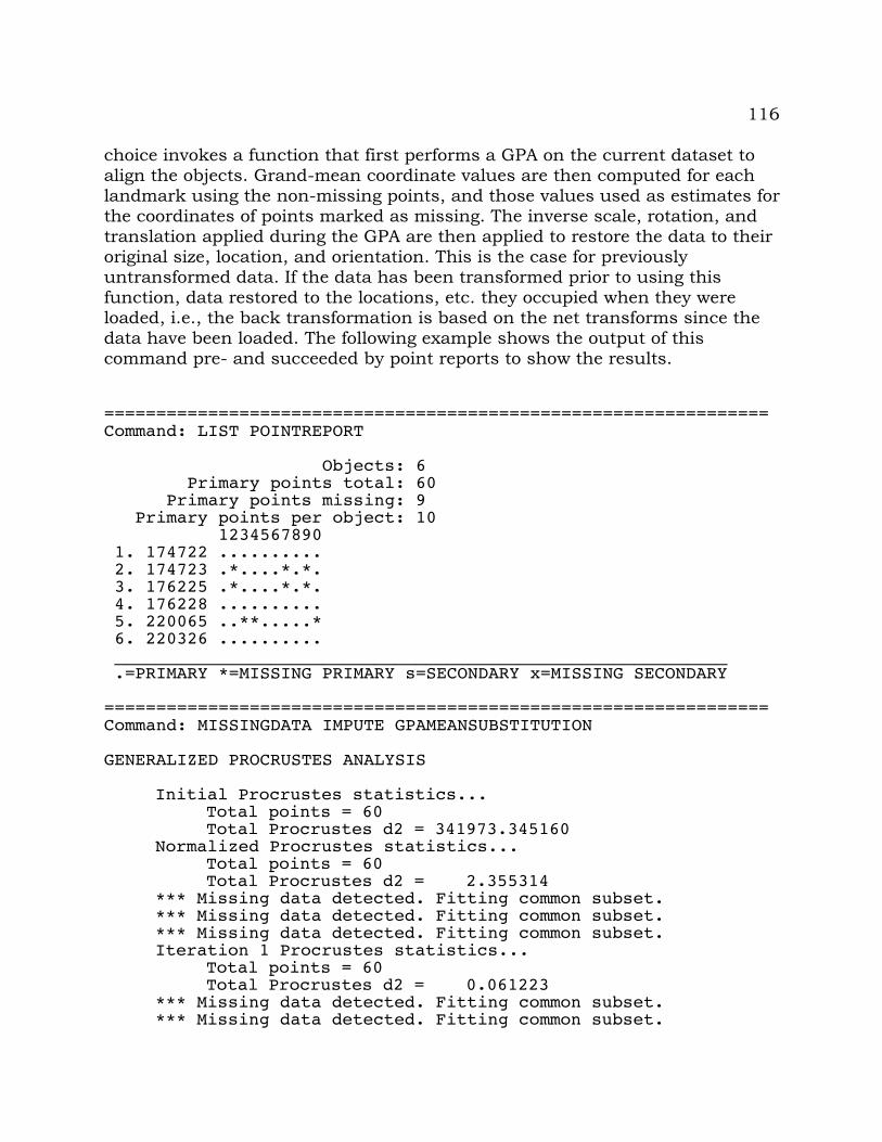
116
choice invokes a function that first performs a GPA on the current dataset to align the objects. Grand-mean coordinate values are then computed for each landmark using the non-missing points, and those values used as estimates for the coordinates of points marked as missing. The inverse scale, rotation, and translation applied during the GPA are then applied to restore the data to their original size, location, and orientation. This is the case for previously untransformed data. If the data has been transformed prior to using this function, data restored to the locations, etc. they occupied when they were loaded, i.e., the back transformation is based on the net transforms since the data have been loaded. The following example shows the output of this command pre- and succeeded by point reports to show the results.
================================================================Command: LIST POINTREPORT
Objects: 6 Primary points total: 60 Primary points missing: 9 Primary points per object: 10 1234567890 1. 174722 .......... 2. 174723 .*....*.*. 3. 176225 .*....*.*. 4. 176228 .......... 5. 220065 ..**.....* 6. 220326 .......... ___________________________________________________________ .=PRIMARY *=MISSING PRIMARY s=SECONDARY x=MISSING SECONDARY
================================================================Command: MISSINGDATA IMPUTE GPAMEANSUBSTITUTION
GENERALIZED PROCRUSTES ANALYSIS
Initial Procrustes statistics...Total points = 60Total Procrustes d2 = 341973.345160
Normalized Procrustes statistics...Total points = 60Total Procrustes d2 = 2.355314
*** Missing data detected. Fitting common subset.*** Missing data detected. Fitting common subset.*** Missing data detected. Fitting common subset.Iteration 1 Procrustes statistics...
Total points = 60Total Procrustes d2 = 0.061223
*** Missing data detected. Fitting common subset.*** Missing data detected. Fitting common subset.
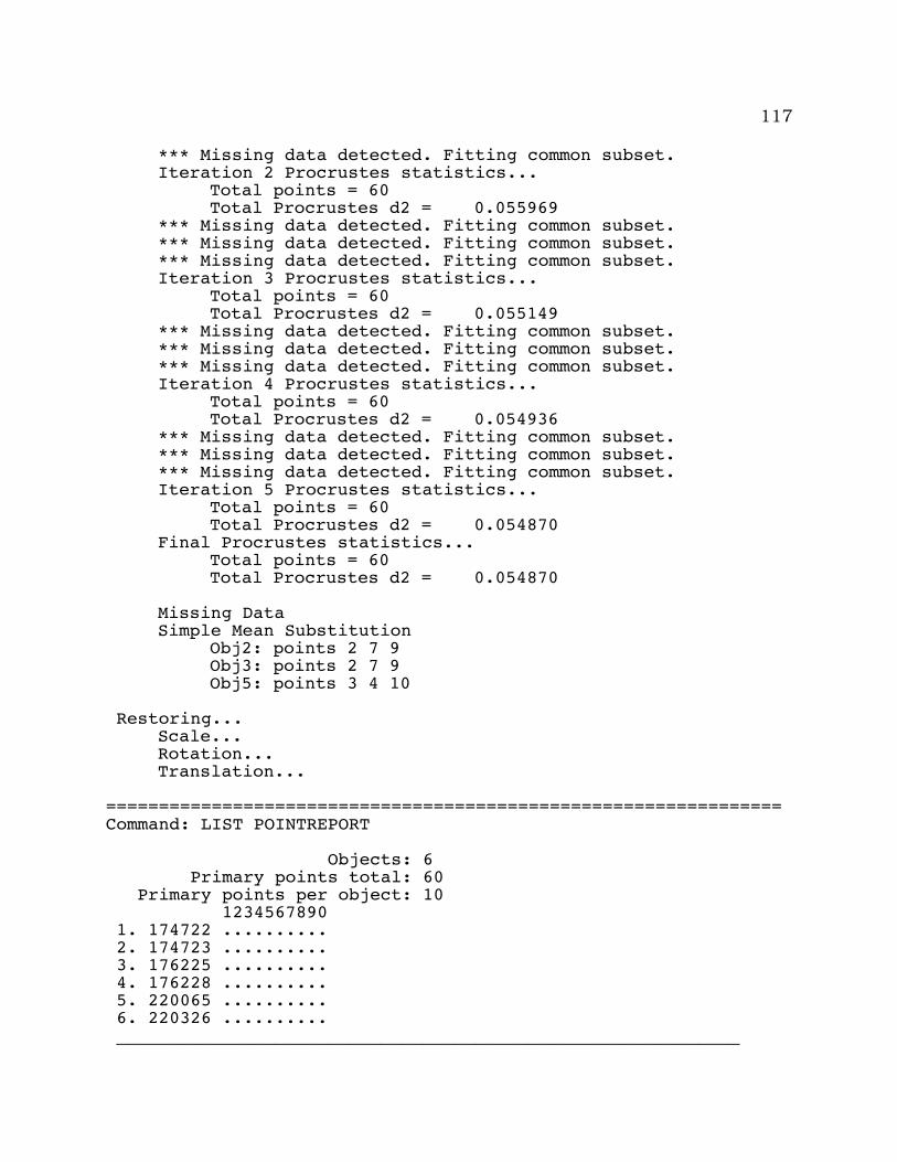
117
*** Missing data detected. Fitting common subset.Iteration 2 Procrustes statistics...
Total points = 60Total Procrustes d2 = 0.055969
*** Missing data detected. Fitting common subset.*** Missing data detected. Fitting common subset.*** Missing data detected. Fitting common subset.Iteration 3 Procrustes statistics...
Total points = 60Total Procrustes d2 = 0.055149
*** Missing data detected. Fitting common subset.*** Missing data detected. Fitting common subset.*** Missing data detected. Fitting common subset.Iteration 4 Procrustes statistics...
Total points = 60Total Procrustes d2 = 0.054936
*** Missing data detected. Fitting common subset.*** Missing data detected. Fitting common subset.*** Missing data detected. Fitting common subset.Iteration 5 Procrustes statistics...
Total points = 60Total Procrustes d2 = 0.054870
Final Procrustes statistics...Total points = 60Total Procrustes d2 = 0.054870
Missing DataSimple Mean Substitution
Obj2: points 2 7 9Obj3: points 2 7 9Obj5: points 3 4 10
Restoring... Scale... Rotation... Translation...
================================================================Command: LIST POINTREPORT
Objects: 6 Primary points total: 60 Primary points per object: 10 1234567890 1. 174722 .......... 2. 174723 .......... 3. 176225 .......... 4. 176228 .......... 5. 220065 .......... 6. 220326 .......... ___________________________________________________________
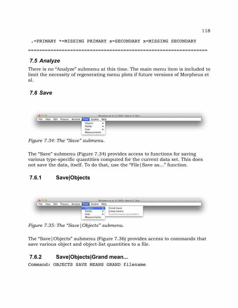
118
.=PRIMARY *=MISSING PRIMARY s=SECONDARY x=MISSING SECONDARY
================================================================
7.5 AnalyzeThere is no “Analyze” submenu at this time. The main menu item is included to limit the necessity of regenerating menu plots if future versions of Morpheus et al.
7.6 Save
The “Save” submenu (Figure 7.34) provides access to functions for saving various type-specific quantities computed for the current data set. This does not save the data, itself. To do that, use the “File|Save as...” function.
7.6.1 Save|Objects
The “Save|Objects” submenu (Figure 7.36) provides access to commands that save various object and object-list quantities to a file.
7.6.2 Save|Objects|Grand mean...Command: OBJECTS SAVE MEANS GRAND filename
Figure 7.34: The “Save” submenu.
Figure 7.35: The “Save|Objects” submenu.
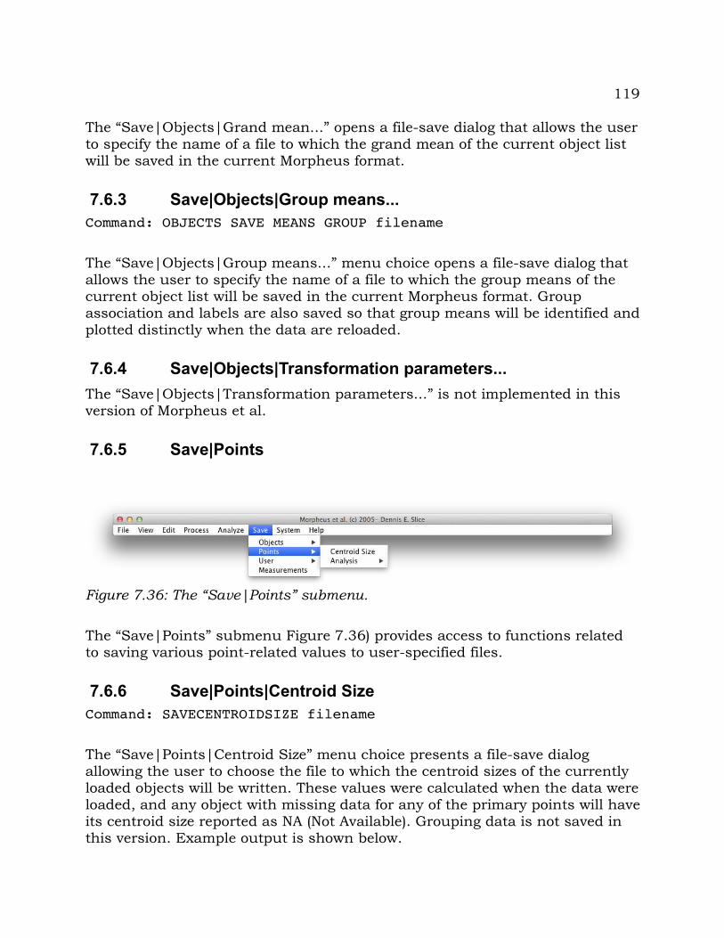
119
The “Save|Objects|Grand mean...” opens a file-save dialog that allows the user to specify the name of a file to which the grand mean of the current object list will be saved in the current Morpheus format.
7.6.3 Save|Objects|Group means...Command: OBJECTS SAVE MEANS GROUP filename
The “Save|Objects|Group means...” menu choice opens a file-save dialog that allows the user to specify the name of a file to which the group means of the current object list will be saved in the current Morpheus format. Group association and labels are also saved so that group means will be identified and plotted distinctly when the data are reloaded.
7.6.4 Save|Objects|Transformation parameters...The “Save|Objects|Transformation parameters...” is not implemented in this version of Morpheus et al.
7.6.5 Save|Points
The “Save|Points” submenu Figure 7.36) provides access to functions related to saving various point-related values to user-specified files.
7.6.6 Save|Points|Centroid SizeCommand: SAVECENTROIDSIZE filename
The “Save|Points|Centroid Size” menu choice presents a file-save dialog allowing the user to choose the file to which the centroid sizes of the currently loaded objects will be written. These values were calculated when the data were loaded, and any object with missing data for any of the primary points will have its centroid size reported as NA (Not Available). Grouping data is not saved in this version. Example output is shown below.
Figure 7.36: The “Save|Points” submenu.
120
================================================================Command: SAVECENTROIDSIZE cs.RData
Ready to write R file...
Centroid sizes for 6 object(s) written to "cs.RData" in "/Users/myaccount/data"================================================================
The following are the contents of the R-formatted file generated by the above command.
# Centroid sizes from /Users/myaccount/data/scapulae.mdt# Jan 19, 2013 4:42:43 AM
# Sample data from:# Taylor, A. B. and D. E. Slice# 2005# A Geometric Morphometric Assessment of the Relationship# between Scapular Variation and Locomotion in African Apes# Pages 299-318 IN# Slice, D. E. (Ed.)# Modern Morphometrics in Physical Anthropology# Kluwer Academic/Plenum Press# REM Three male Gorilla gorilla gorilla# Three male Pan troglodytes.# REM Images contrast enhanced.# REM Notice images carry scale factors from tpsDig.# *File format version no.# *Point 1 made missing for object 3# *File format version no.
CENTROID_SIZE"174722" 329.315534"174723" 313.577934"176225" NA"176228" 226.825204"220065" 211.392596"220326" 222.377599
7.6.7 Save|Points|Analysis
121
The “Save|Points|Analysis” submenu (Figure 7.37) currently contains no items. It is included as a placeholder for future functions.
7.6.8 Save|User
The “Save|User” submenu (Figure 7.38) currently contains no items. It is included as a placeholder for future functions.
7.6.9 Save|Measurements...Command: MEA SAVE filename
The “Save|Measurements...” choice opens a file-save dialog allowing the user to specify the location and name of the file to which to output the current measurement values. The values are saved in R format and can be read directly into R with the “read.table()” command. The first row of the file contains the labels for the columns of data. Subsequent rows begin with a number indicating the object followed by the object's label and the computed values for each measurement. An example follows.
================================================================Command: MEA SAVE mea.RData
Measurements saved to /Users/myaccount/data/mea.RData
================================================================
Figure 7.37: The “Save|Points|Analysis” submenu.
Figure 7.38: The “Save|User” submenu.
122
The contents of one such output file is shown below for a data set that had two distances, D1 and D2, and one angle, A1, defined. The first variable is the object label. Note that the group index and label are also included if the data have been grouped. Also, the second specimen had missing data for a landmark necessary to compute the D1 and A1 measurements. Its values are thus marked as NA – the R reserved word for “Not Available”.
Object GroupI GroupLabel "D1" "D2" "A1" 1 "174722" 1 Gorilla 123.757428 113.210279 0.1502842 "174723" 1 Gorilla NA 92.041595 NA3 "176225" 1 Gorilla 130.940010 127.380697 0.3972584 "176228" 2 Pan 84.261020 53.148582 0.3954605 "220065" 2 Pan 73.889144 63.434751 0.4124196 "220326" 2 Pan 87.256977 58.968477 0.388476
7.7 System
The “System” submenu (Figure 7.39) provides access to submenus and options related to the program desktop appearance, text output, and other program-wide parameters. Some parameters related to desktop appearance are stored in the Morpheus configuration file.
7.7.1 System|Stop graphics updateThe “System|Stop graphics update” toggle, when checked, turns off the automatic updating of plots by the program. Refreshing plots can be very time consuming when dealing with large data sets such as those including surface meshes. In fact, refreshing can be the most time consuming aspect of a given computation. After the computations have completed, unchecking this toggle will force the graphics to refresh and automatic refreshing by the program will resume.
7.7.2 System|Desktop
Figure 7.39: The “System” submenu.
123
The “System|Desktop” submenu (Figure 7.40) provides access to options that affect the appearance of the main program window.
7.7.3 System|Deskptop|Size...The “System|Desktop|Size...” menu choice presents the user with a dialog in which they can specify the exact dimensions of the program window. This is most useful for, say, preparing graphics and figures of consistent size and resolution for publication. All menu figures in this manual, for instance, used a program desktop width of 1024 pixels. Figure 7.41 shows the “System|Desktop|Size...” dialog.
Figure 7.41: The “System|Desktop|Size...” dialog.
7.7.4 System|Desktop|DefaultsThe “System|Desktop|Defaults” menu choice resizes the main program window to the default size computed at startup.
7.7.5 System|Parameters
Figure 7.40: The “System|Desktop” submenu.
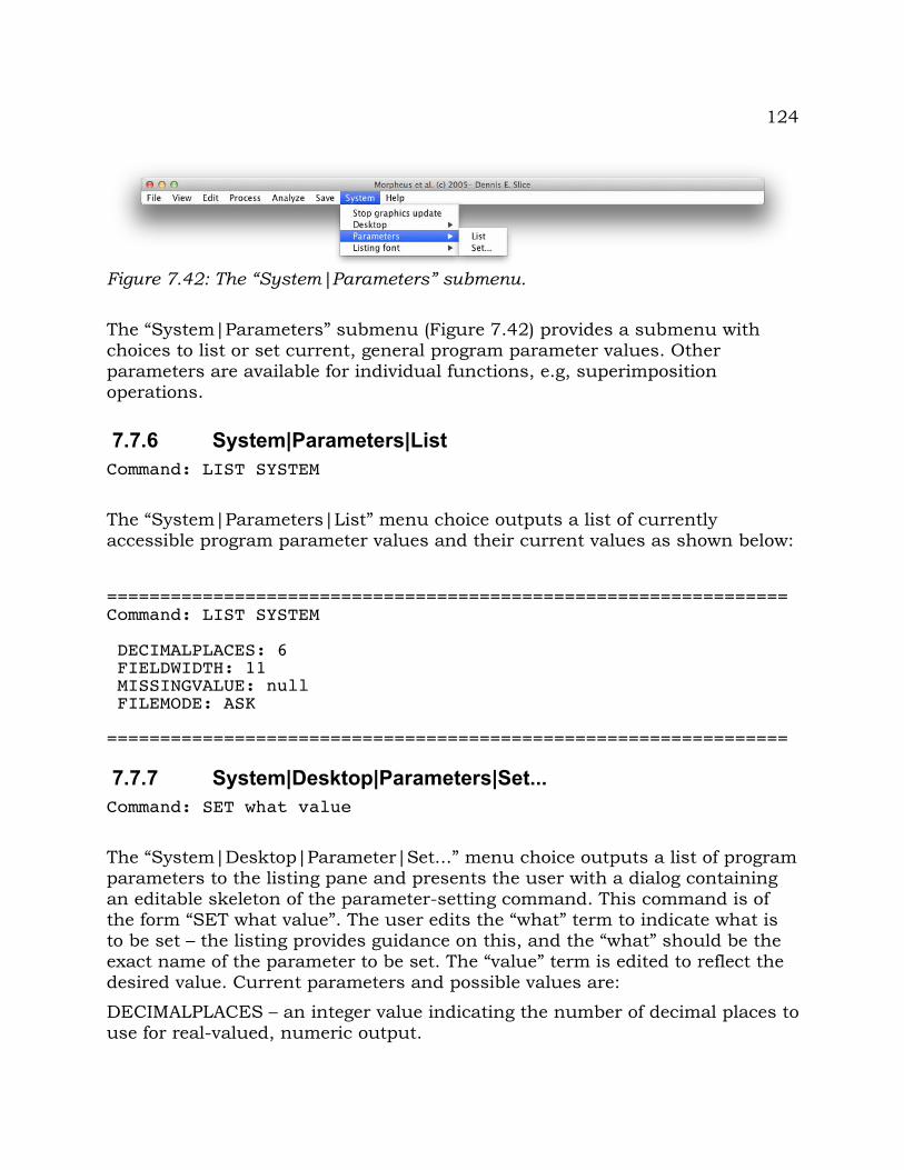
124
The “System|Parameters” submenu (Figure 7.42) provides a submenu with choices to list or set current, general program parameter values. Other parameters are available for individual functions, e.g, superimposition operations.
7.7.6 System|Parameters|ListCommand: LIST SYSTEM
The “System|Parameters|List” menu choice outputs a list of currently accessible program parameter values and their current values as shown below:
================================================================Command: LIST SYSTEM
DECIMALPLACES: 6 FIELDWIDTH: 11 MISSINGVALUE: null FILEMODE: ASK
================================================================
7.7.7 System|Desktop|Parameters|Set...Command: SET what value
The “System|Desktop|Parameter|Set...” menu choice outputs a list of program parameters to the listing pane and presents the user with a dialog containing an editable skeleton of the parameter-setting command. This command is of the form “SET what value”. The user edits the “what” term to indicate what is to be set – the listing provides guidance on this, and the “what” should be the exact name of the parameter to be set. The “value” term is edited to reflect the desired value. Current parameters and possible values are:
DECIMALPLACES – an integer value indicating the number of decimal places to use for real-valued, numeric output.
Figure 7.42: The “System|Parameters” submenu.
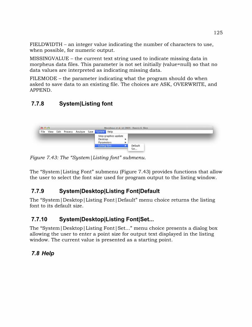
125
FIELDWIDTH – an integer value indicating the number of characters to use, when possible, for numeric output.
MISSINGVALUE – the current text string used to indicate missing data in morpheus data files. This parameter is not set initially (value=null) so that no data values are interpreted as indicating missing data.
FILEMODE – the parameter indicating what the program should do when asked to save data to an existing file. The choices are ASK, OVERWRITE, and APPEND.
7.7.8 System|Listing font
The “System|Listing Font” submenu (Figure 7.43) provides functions that allow the user to select the font size used for program output to the listing window.
7.7.9 System|Desktop|Listing Font|DefaultThe “System|Desktop|Listing Font|Default” menu choice returns the listing font to its default size.
7.7.10 System|Desktop|Listing Font|Set...The “System|Desktop|Listing Font|Set...” menu choice presents a dialog box allowing the user to enter a point size for output text displayed in the listing window. The current value is presented as a starting point.
7.8 Help
Figure 7.43: The “System|Listing font” submenu.
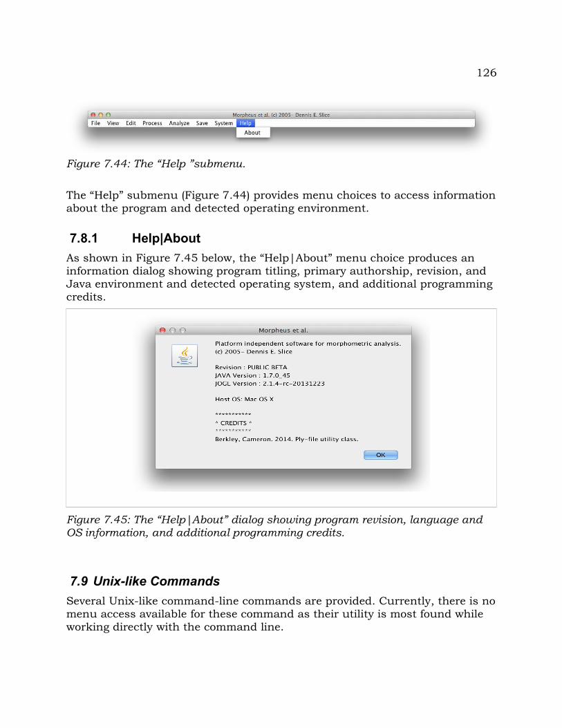
126
The “Help” submenu (Figure 7.44) provides menu choices to access information about the program and detected operating environment.
7.8.1 Help|AboutAs shown in Figure 7.45 below, the “Help|About” menu choice produces an information dialog showing program titling, primary authorship, revision, and Java environment and detected operating system, and additional programming credits.
Figure 7.45: The “Help|About” dialog showing program revision, language and OS information, and additional programming credits.
7.9 Unix-like CommandsSeveral Unix-like command-line commands are provided. Currently, there is no menu access available for these command as their utility is most found while working directly with the command line.
Figure 7.44: The “Help ”submenu.
127
7.9.1 lsCommand: LS filename
The file listing command, LS, outputs the names of the contents (files and directories) in the current, working directory to the listing window. Basic wildcards such as '*' and '?' are supported. The following shows a simple example.
N.B. Wildcards appear not to work. This has been added to the TODO list for a future version.
================================================================Command: LS *.mdt
/Users/myaccount/data/3d.DS_Storemandible.mdtmandible.objmea3d.mdtsurfaces_with_points.mdtwilliams.mdt
================================================================
7.9.2 pwdCommand: PWD
The print working directory command, PWD, outputs the current working directory to the listing window. The current, working directory is the last directory from which a data file was read or written by Morpheus. An example is shown below.
================================================================Command: PWD
/Users/myaccount/data================================================================
7.9.3 clsCommand: CLS
For clear screen command, CLS, clears the Morpheus listing window.

128
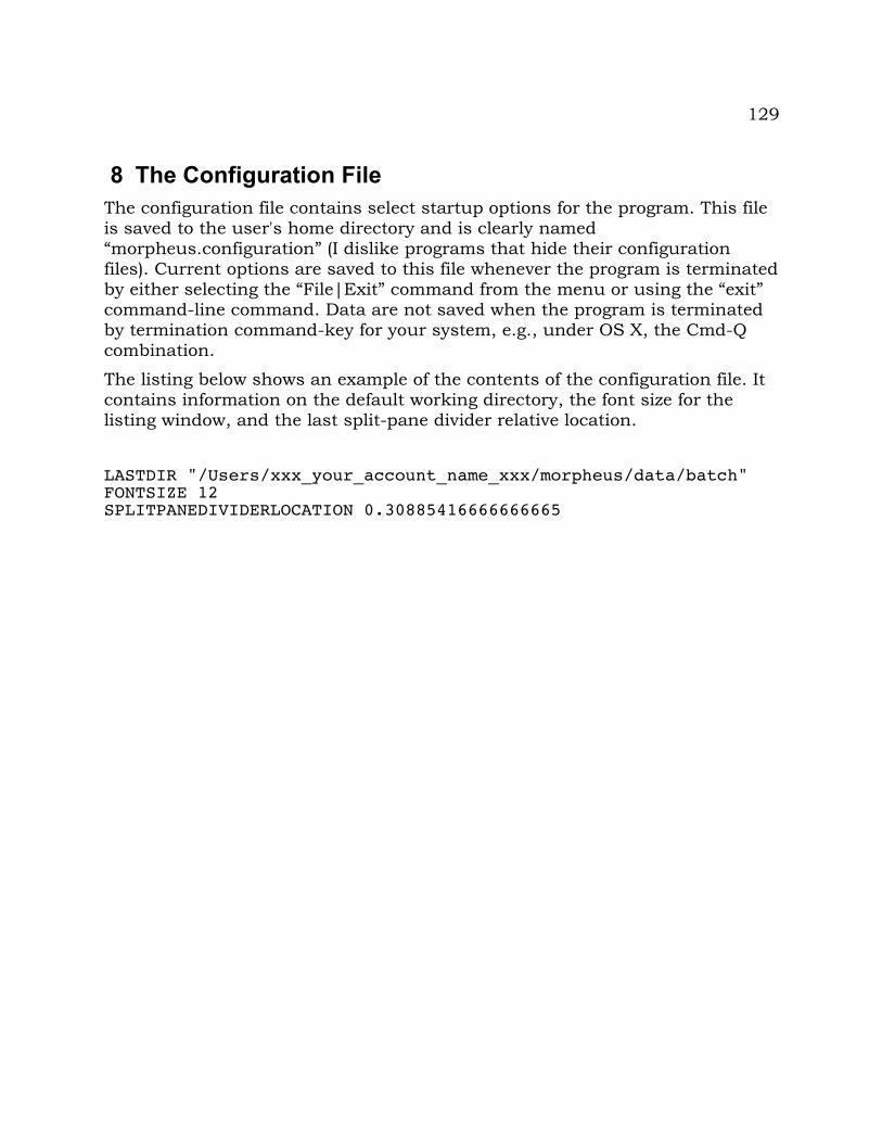
129
8 The Configuration FileThe configuration file contains select startup options for the program. This file is saved to the user's home directory and is clearly named “morpheus.configuration” (I dislike programs that hide their configuration files). Current options are saved to this file whenever the program is terminated by either selecting the “File|Exit” command from the menu or using the “exit” command-line command. Data are not saved when the program is terminated by termination command-key for your system, e.g., under OS X, the Cmd-Q combination.
The listing below shows an example of the contents of the configuration file. It contains information on the default working directory, the font size for the listing window, and the last split-pane divider relative location.
LASTDIR "/Users/xxx_your_account_name_xxx/morpheus/data/batch"FONTSIZE 12SPLITPANEDIVIDERLOCATION 0.30885416666666665

130
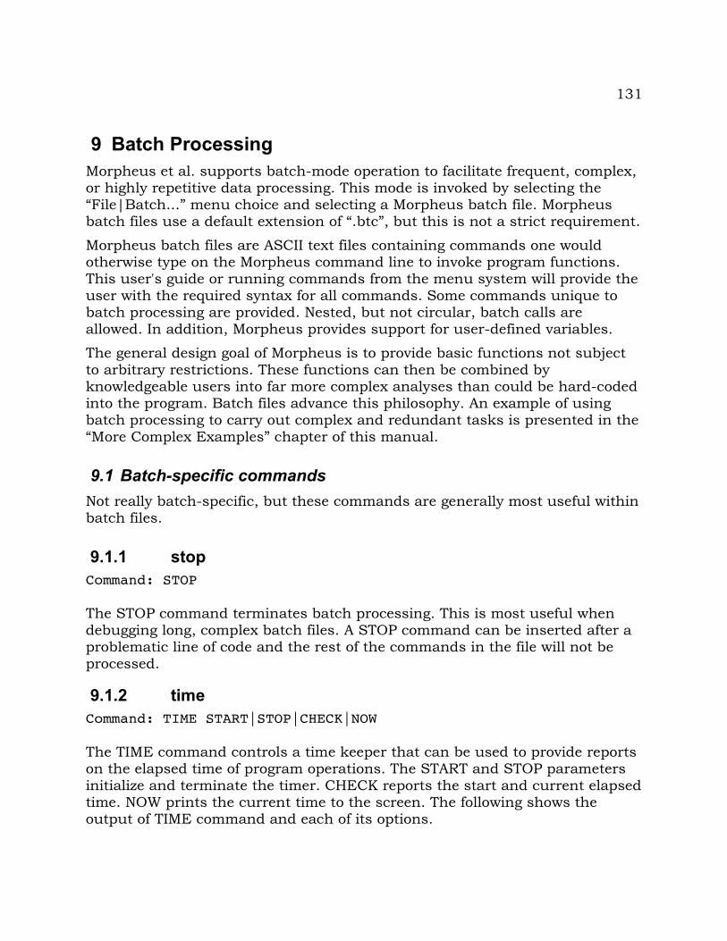
131
9 Batch ProcessingMorpheus et al. supports batch-mode operation to facilitate frequent, complex, or highly repetitive data processing. This mode is invoked by selecting the “File|Batch...” menu choice and selecting a Morpheus batch file. Morpheus batch files use a default extension of “.btc”, but this is not a strict requirement.
Morpheus batch files are ASCII text files containing commands one would otherwise type on the Morpheus command line to invoke program functions. This user's guide or running commands from the menu system will provide the user with the required syntax for all commands. Some commands unique to batch processing are provided. Nested, but not circular, batch calls are allowed. In addition, Morpheus provides support for user-defined variables.
The general design goal of Morpheus is to provide basic functions not subject to arbitrary restrictions. These functions can then be combined by knowledgeable users into far more complex analyses than could be hard-coded into the program. Batch files advance this philosophy. An example of using batch processing to carry out complex and redundant tasks is presented in the “More Complex Examples” chapter of this manual.
9.1 Batch-specific commandsNot really batch-specific, but these commands are generally most useful within batch files.
9.1.1 stopCommand: STOP
The STOP command terminates batch processing. This is most useful when debugging long, complex batch files. A STOP command can be inserted after a problematic line of code and the rest of the commands in the file will not be processed.
9.1.2 timeCommand: TIME START|STOP|CHECK|NOW
The TIME command controls a time keeper that can be used to provide reports on the elapsed time of program operations. The START and STOP parameters initialize and terminate the timer. CHECK reports the start and current elapsed time. NOW prints the current time to the screen. The following shows the output of TIME command and each of its options.
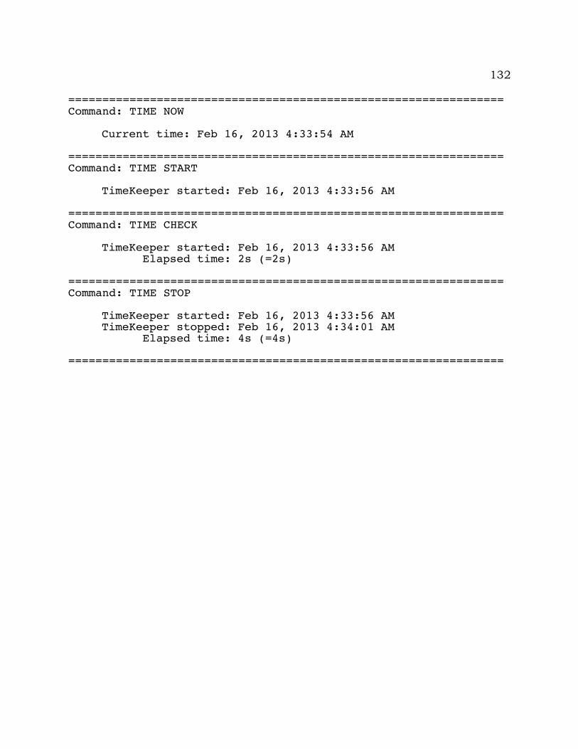
132
================================================================Command: TIME NOW
Current time: Feb 16, 2013 4:33:54 AM
================================================================Command: TIME START
TimeKeeper started: Feb 16, 2013 4:33:56 AM
================================================================Command: TIME CHECK
TimeKeeper started: Feb 16, 2013 4:33:56 AM Elapsed time: 2s (=2s)
================================================================Command: TIME STOP
TimeKeeper started: Feb 16, 2013 4:33:56 AMTimeKeeper stopped: Feb 16, 2013 4:34:01 AM Elapsed time: 4s (=4s)
================================================================

133
10 Morpheus Data Files (.mdt)The native, default format of newer versions of the program is a slightly extended version of that used by the old Morpheus et al. The format was developed to be flexible, extensible, and human-readable. The “object” represents the level of the individual specimen, and data or parameters provided outside of an object specification, such as links or measurements, are associated with all objects in the data set. In general, the ordering of complete units of data, such as complete point specifications, curves, etc., is irrelevant within an object (though in practice, it must be consistent throughout the data set), as are spacing, line breaks (with some exceptions), etc. The basic structure of the data specification is that of a tag followed by a label followed by information appropriate to that data type. Files must be ASCII text files – not Word or OpenOffice document files.
Note, the Morpheus format is very easy to read, but rather difficult to construct. It is often convenient to get data into Morpheus by initially importing it from a simpler format. The author often uses the NTSYS format described later for this purpose.
The following is an example of a two-dimensional Morpheus data set. It is a rather confused jumble since it was designed to test I/O robusticity. “...snip...” indicates lines deleted to save space. Details are discussed below:
REM *1 2-dimensional object loaded from f:\m\data\one.mdt.REM *DATE: 1996-06-23 TIME: 14.47.27
DIM 2MISSING -999
REM Sample data file for testing morpheus data structure input
OBJ "FIGURE 517" USERCHAR "sex" M P "First point" 94.740 922.490 USERTEXT "Source" CMNH USERTEXT "Source" "Carnegie Museum of Natural History" P "Second point" 531.580 1211.240 P "" 855.260 1456.560 P "" 836.840 1275.130 REM next val P "" 1050.00 1086.03 USERINT "Number of eyes" 2 P "test missing" -999 -999 ...snip... P "" 1936.840 567.290 USERDBL "" 128.340 P "" 136.840 746.170
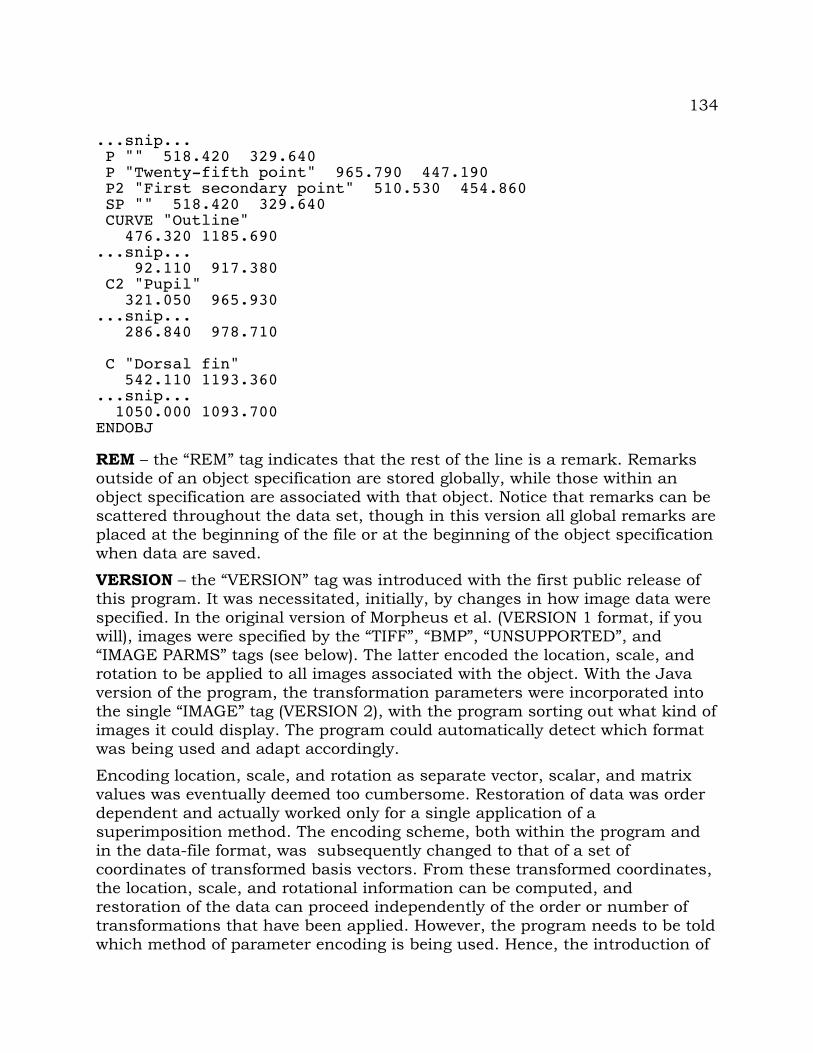
134
...snip... P "" 518.420 329.640 P "Twenty-fifth point" 965.790 447.190 P2 "First secondary point" 510.530 454.860 SP "" 518.420 329.640 CURVE "Outline" 476.320 1185.690 ...snip... 92.110 917.380 C2 "Pupil" 321.050 965.930 ...snip... 286.840 978.710
C "Dorsal fin" 542.110 1193.360 ...snip... 1050.000 1093.700 ENDOBJ
REM – the “REM” tag indicates that the rest of the line is a remark. Remarks outside of an object specification are stored globally, while those within an object specification are associated with that object. Notice that remarks can be scattered throughout the data set, though in this version all global remarks are placed at the beginning of the file or at the beginning of the object specification when data are saved.
VERSION – the “VERSION” tag was introduced with the first public release of this program. It was necessitated, initially, by changes in how image data were specified. In the original version of Morpheus et al. (VERSION 1 format, if you will), images were specified by the “TIFF”, “BMP”, “UNSUPPORTED”, and “IMAGE PARMS” tags (see below). The latter encoded the location, scale, and rotation to be applied to all images associated with the object. With the Java version of the program, the transformation parameters were incorporated into the single “IMAGE” tag (VERSION 2), with the program sorting out what kind of images it could display. The program could automatically detect which format was being used and adapt accordingly.
Encoding location, scale, and rotation as separate vector, scalar, and matrix values was eventually deemed too cumbersome. Restoration of data was order dependent and actually worked only for a single application of a superimposition method. The encoding scheme, both within the program and in the data-file format, was subsequently changed to that of a set of coordinates of transformed basis vectors. From these transformed coordinates, the location, scale, and rotational information can be computed, and restoration of the data can proceed independently of the order or number of transformations that have been applied. However, the program needs to be told which method of parameter encoding is being used. Hence, the introduction of
135
the “VERSION” tag starting with version 3, e.g. “VERSION 3”. This will also allow subtle adjustments to the file format in the future.
It is recommended that the “VERSION” tag be placed in the data file either before or after any initial comments. This is the convention now used by the program for saving morpheus-formatted data.
DIM – the “DIM” specification is optional for two-dimensional data. Otherwise, it is required to specify the dimensionality of the data to follow. Any non-zero integer following the tag is acceptable.
MISSING – if the data have missing values encoded in them, the “MISSING” tag can be used to specify the value indicating that data is missing. This can be either a number, integer, or string (e.g., a dot, '.'). Morpheus first tries to convert the value into a number. If that succeeds, subsequent attempts to read in data that could be missing are compared numerically to the missing value. If the specified missing value cannot be converted to a numerical value, a string comparison is made between data tokens read in by the program and the missing value. In either case, if match is found, the particular data being read in is marked as missing. Examples of frequently used values include “999”, “-999”, '.'
OBJ – the “OBJ” tag marks the beginning of data for a new specimen or object. It must be followed by an object label. Labels with spaces can be specified in quotes, and blank labels in quotes are acceptable. Between an “OBJ” tag and the “ENDOBJ” or the next “OBJ” tag are the data for that object.
POINT, P – the fundamental data type in current geometric morphometric analysis is the location of an anatomical point, or landmark, specified by its Cartesian coordinates. Morpheus recognizes two types of points – primary and secondary. Primary points are the ones used in point-related parameter computations such as those of generalized Procrustes analysis, etc. Secondary points are merely carried along by any transformations and can be used to isolate an analysis to a specific subset of points or simply for visualization. The “POINT” or “P” tag indicates a primary point. It must be followed by a label, such as “bregma”, but a blank label can be specified by empty quotes. This is followed by the number of numerical values specified by the dimensionality of the data. Labels and/or coordinates must be in order, but need not occupy the same line.
P2, SP – secondary points are indicated by either the tags “P2” or “SP”. As described under the “P” tag definition, secondary points are carried along with data transformations, but are not used in the computation of transformation parameters or subsequent statistical analysis. In the original Morpheus, primary and secondary points were two different types of data. Now, “primary” and “secondary” are treated as attributes of individual points.
136
CURVE, C – besides points, Morpheus also supports the specification of curves in n-dimensions. These are indicated by either the “CURVE” or “C” tag followed by a label. These are then followed by an arbitrary number of sets of point coordinates that describe the curve. The end of the curve is indicated when the next tag or end-of-file is found. As with points, both primary and secondary curves are supported. Their distinct usage at this point remains a mystery even to the development team.
C2, SC – the “C2” and “SC” tags indicate specification of a secondary curve. The formatting is otherwise the same as for primary curves.
USERCHAR, USERTEXT, USERINT, USERDBL – a variety of data types are provided to record non-coordinate user data such as sex, museum, size, etc. For each variable, one of these tags must be provided and followed by a label. Again, blank labels can be indicated by empty quotation marks. The label is then followed by appropriate data. “USERCHAR” is used for data consisting of a single character code, e.g., USERCHAR “sex” m. “USERTEXT” is used for more lengthy text descriptors, e.g., USERTEXT “location” south_america or USERTEXT “location” “south america”. “USERINT” types can hold integer values, e.g., USERINT “bristle number” 7. And “USERDBL” can be used to record real-valued variables (sorry, the tag derives from the use of 'double' in programming terms to indicate double-precision real numbers), e.g., USERDBL “mass” 260.5.
ENDOBJ – this is an optional tag included for neatness and indicates the end of the data specification for an object. The program will actually recognize the end of an object specification when it finds another “OBJ” tag or end-of-file marker.
TIFF, BMP, UNSUPPORTED, IMAGEPARMS – (NOTE: this form of image specification is still supported, but should not be used) “TIFF”, “BMP”, and “UNSUPPORTED” were tags used in the old Morpheus to identify images associated with an object. The old Morpheus was capable of displaying TIFF and BMP images, and in UNSUPPORTED cases would save the image filename to keep it associated with the object. For consistency, these tags must be followed by a label, even a blank one, and then by the name of the image file with quotes included as needed to allow for spaces in the path or filename. If a complete path is not included, the images are assumed to be relative to the current directory. IMAGEPARMS is a tag for providing scale, translation, and rotation information (as an angle) for 2D images. These parameters would be associated with all images in an object and provided the necessary information to transform images along with points as they were, say, subjected to GPA. In fact, the original Morpheus was never able to rotate the images, but would apply the scaling and translation parameters to provide some approximation to the actual transform (the newer Morpheus versions do apply all of the transforms). Below is an example of an object with a BMP image and an image
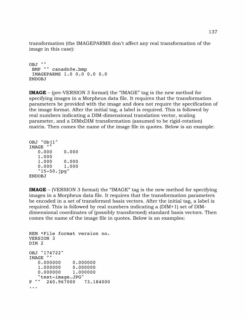
137
transformation (the IMAGEPARMS don't affect any real transformation of the image in this case):
OBJ "" BMP "" canadn0e.bmp IMAGEPARMS 1.0 0.0 0.0 0.0ENDOBJ
IMAGE – (pre-VERSION 3 format) the “IMAGE” tag is the new method for specifying images in a Morpheus data file. It requires that the transformation parameters be provided with the image and does not require the specification of the image format. After the initial tag, a label is required. This is followed by real numbers indicating a DIM-dimensional translation vector, scaling parameter, and a DIMxDIM transformation (assumed to be rigid-rotation) matrix. Then comes the name of the image file in quotes. Below is an example:
OBJ "Obj1"IMAGE "" 0.000 0.000 1.000 1.000 0.000 0.000 1.000 "15-50.jpg"ENDOBJ
IMAGE – (VERSION 3 format) the “IMAGE” tag is the new method for specifying images in a Morpheus data file. It requires that the transformation parameters be encoded in a set of transformed basis vectors. After the initial tag, a label is required. This is followed by real numbers indicating a (DIM+1) set of DIM-dimensional coordinates of (possibly transformed) standard basis vectors. Then comes the name of the image file in quotes. Below is an examples:
REM *File format version no.VERSION 3DIM 2
OBJ "174722"IMAGE "" 0.000000 0.000000 1.000000 0.000000 0.000000 1.000000 "test-image.JPG"P "" 240.967000 73.184000 ...

138
ENDOBJ
SURFACE, SURF – the “SURFACE” or “SURF” tag indicates the specification of an surface file. Logically, this could be considered a three-dimensional image file, but such data required a bit too much specialized programming to be easily incorporated under the IMAGE tag for now. Like the IMAGE tag, the SURF tag requires a label, then translation, scale, and rotation/transformation matrix specification. Wavefront .obj and .ply (polygon) files are supported at this time (see description under “Surface Formats” below),. The following are examples of the use of the SURF tag in both the VERSION 3 and pre-VERSION 3 formats:
VERSION 3...VERSION 3DIM 3OBJ "mandible"SURF "" 0.0 0.0 0.0 1.0 0.0 0.0 0.0 1.0 0.0 0.0 0.0 1.0 "mandible.obj"ENDOBJ
REM *File format version no.VERSION 3DIM 3
OBJ "mandible"SURF "" 0.127366 0.049117 0.014852 0.131988 0.049117 0.014852 0.127366 0.053739 0.014852 0.127366 0.049117 0.019474 "mandible.obj"P "" -0.004051 -0.029724 0.036688 ...ENDOBJ
Pre-VERSION 3...DIM 3OBJ "mandible"SURF "" 0.0 0.0 0.0
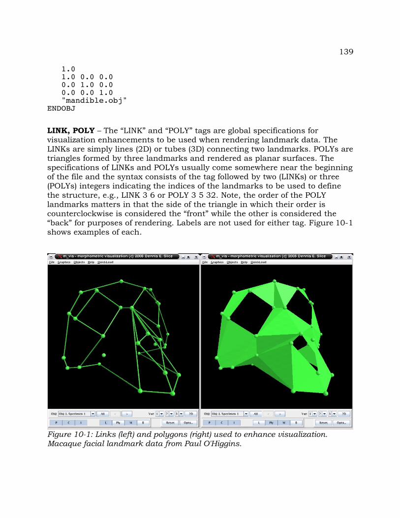
139
1.0 1.0 0.0 0.0 0.0 1.0 0.0 0.0 0.0 1.0 "mandible.obj"ENDOBJ
LINK, POLY – The “LINK” and “POLY” tags are global specifications for visualization enhancements to be used when rendering landmark data. The LINKs are simply lines (2D) or tubes (3D) connecting two landmarks. POLYs are triangles formed by three landmarks and rendered as planar surfaces. The specifications of LINKs and POLYs usually come somewhere near the beginning of the file and the syntax consists of the tag followed by two (LINKs) or three (POLYs) integers indicating the indices of the landmarks to be used to define the structure, e.g., LINK 3 6 or POLY 3 5 32. Note, the order of the POLY landmarks matters in that the side of the triangle in which their order is counterclockwise is considered the “front” while the other is considered the “back” for purposes of rendering. Labels are not used for either tag. Figure 10-1 shows examples of each.
Figure 10-1: Links (left) and polygons (right) used to enhance visualization. Macaque facial landmark data from Paul O'Higgins.
140
DIST, ANGL, TRIAREA, ARCL, PERI, AREA – These tags specify measurements to be made on all objects. Like LINKs and POLYs, these are global specifications and are usually found near the top of the file. After each tag is a label that is followed by the appropriate number of integers specifying the landmarks or curves to be used in the computation. Examples of each follow. Comments in parentheses would not be included in an actual data file:
DIST “head_length” 1 7 (distance between points one and seven)ANGL “face_angle” 3 9 17 (angle at point nine formed with points three and seventeen)TRIAREA “facial_area” 3 9 17 (area of the triangle formed by points three, nine, and seventeen)ARCL “brow arc” 3 (arclength of curve number three)PERI “skull perimeter” 1 (perimeter of curve one – arclength plus distance from first and last point)AREA “orbital area” 2 (area of curve two – two dimensional data only)
CMD – the “CMD” tag indicates a line containing an embedded Morpheus command that should be applied to the data after loading. Currently, two commands are supported - “GROUP” and “LABEL”. The GROUP command groups the data, while the LABEL command applies labels to the groups. See the “Commands” chapter for details, but simple examples of each are: “GROUP 52 45” that groups the data such that the first fifty-two objects are in group one, the next forty-five are in group two, and any remaining objects are in group three, and “LABEL male female juvenile”, which would relabel the three groups from the previous command “male”, “female”, and “juvenile”. Default group labels are of the form “gi:j” where “i” is the group number and “j” is the group size. An embedded LABEL command must appear after an embedded GROUP command. For instance:
CMD GROUP 52 45CMD LABEL male female juvenile
141
11 Other Morpheus FormatsMorpheus supports one or more other formats to associate different types of data with the specimens in a Morpheus data file. These are described below.
11.1 Morpheus grouping files (.grp)Besides grouping specimens by count, one can also group them by a list of tags provided in a Morpheus grouping file. Count grouping, of course, requires all group members be contiguously arranged within the file. Grouping files allow alternative groupings. The format of the file is rather simple. There may be any number of comment lines, indicated by “REM” tags, scattered throughout the file. Non-blank, non-remark lines that contain text are treated as group labels. The text may be integers, real numbers, characters, or strings. All such data are read as strings, and the number of unique strings in such a file determines the number of groups. Each individual, in order, is assigned to the group indicated by the grouping string. Note, there must be exactly as many non-blank, non-comment lines in the grouping file as the number of objects being grouped. The “.grp” suffix is used for convenience, but is not required. Below is part of a grouping file:
REM grouping for 10 individuals.REM 3 groupsREM malemmREM femalefmfffREM juvenile3m3
This file can be used to group ten objects as “m” for male, “f” for female, and “3” for juvenile. The mix of characters and integers is meant to show the flexibility of the grouping system and emphasize that numbers are treated as strings for purposes of identifying groups and associating objects.

142
143
12 Other Supported Data Formats
12.1 Integrate (.lnd)Support for the Integrate format was developed as part of a consulting project to read in a specific set of data files. Perhaps it could be useful to others. The files are ASCII text with the following structure (ellipses “...” indicated lines deleted to save space):
SUBJECT_ID = UnnamedSCAN_TYPE = NO TYPESTUDY_NAME = * * * NO STUDY * * *LAND_STUDY = New StudySTD_LAND = 42AUX_LAND = 6STANDARD = 1 259 212 78.59 -78.54 148.40 -2.90...42 -999 -999 0.00 0.00 0.00 0.00AUX = 1 -999 -999 0.00 0.00 0.00 0.00 top_head... 6 161 85 144.22 -56.83 59.50 132.56 chinEND =
The import routine was developed from looking at a series of these files, so it simply imports the initial tokens on the first four lines as named USERTEXT variables. The rest of the line after the '=' is read in as the value. The number of standard landmarks, n, is then read in and then the number of auxiliary landmarks, m. The next line is skipped, and n standard lines are read. The first token on each line is used as the point label, the next three are skipped, and the final three read in as x, y, and z coordinates. The next line is skipped, and M auxiliary landmarks are read in. Here, the first four tokens are skipped and the rest of the line after the z coordinate is read in as a point label, e.g., “top_head” and “chin” above.
It is assumed that “-999” indicates missing values. Standard points are flagged as “primary” points, and auxiliary points are flagged as “secondary”.
I am not sure how common this format is, but if you have some Integrate files with standard and auxiliary landmarks, this should read them in. If you have a variation on this that you would like to see supported, feel free to contact the Morpheus development team.

144
12.2 Morphologika (.txt)Morphologika (see https://sites.google.com/site/hymsfme/resources ) is the morphometrics program developed by Paul O'Higgins and Nicholas Jones5. It supported 3D data and has embedded PCA analysis with scatter plots and visualization of associated morphologies. Below is the provided 3D example data file used to develop support in Morpheus. “...snip...” indicates data deleted to save space. Changes to support 2D data are obvious:
[individuals]15[landmarks]31[Dimensions]3[names]Specimen 1...snip...Specimen 15[labels]Sex[labelvalues]Female...snip...MaleFemale[rawpoints]'#116.01 24.17 11.18...snip...17.48 27.52 13.71...snip...'#15 22.44 25.44 10.9...snip...23.63 29.14 13.63[wireframe]1 4...snip...15 31[polygons]8 6 7 ...snip...18 30 17
5 Morphologika is reportedly no longer developed or maintained. The user is, instead, directed to EVAN toolkit – http://www.evan-society.org/.
145
Morphologika tags are contained in square brackets and followed by relevant data. The first three of these indicate the number of individuals and landmarks in the file and the dimensionality of the coordinate data. Next, come the names for each specimen and a label for one or more user-supplied variables. This is followed by the values of the labeled variables. These values must match the variable names and number of individuals previously specified. After the label values are the raw coordinates for each landmark in each individual. The lines beginning with a single quote in the rawpoints section are interpreted by Morpheus as object-level remarks. Wireframes are Morphologika's equivalent of Morpheus links, and that tag is followed by an arbitrary number of integer pairs specifying the numbers of the landmarks to be linked. Similarly, polygons are triplets of points that define triangles used to help visualize three-dimensional structures. See the Morphologika documentation for more detail.
12.3 R (.Rdata)The R format is used to export data (group label and indices, user variables, and primary point coordinates) into an ASCII text file that can be read directly into the R program with the “read.table('filename')” command. Column labels are provided on the first row, then the coordinate or other data. Coordinates for each primary point are provided on a single row for each object, and this row begins with a row label. When R attempts to read the file, it will recognize the first line has one less column that the next and interpret this as indicating the first row contains column-label information. An example follows where “...snip...” indicates data excised to save space:
"P1.1" "P1.2" "P1.3" ...snip... "P8.1" "P8.2" "P8.3" "Obj1" 1.000 1.000 1.000 ...snip... 1.000 -1.000 -1.000 "Obj2" 1.000 1.000 1.000 ...snip... 1.000 -1.000 -1.000 ...snip..."Obj9" 0.410 0.410 0.410 ...snip... 0.410 -0.410 -0.410
If the points have associated labels, these are used to generate the column labels. Otherwise, “Pi” is used, where i indicates the point number. Appended to these are the dimension number, e.g., “.1”, “.2”, etc. Object labels are used as row labels if they exist. Otherwise, row labels are generated as “Objj”, where j indicates the object number. The above example is for nine, three dimensional objects (cubes) with eight landmarks.
This format is also used for other exported information such as measurement values. These can be read in and merged with coordinate or other compatible
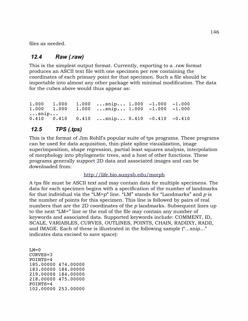
146
files as needed.
12.4 Raw (.raw)This is the simplest output format. Currently, exporting to a .raw format produces an ASCII text file with one specimen per row containing the coordinates of each primary point for that specimen. Such a file should be importable into almost any other package with minimal modification. The data for the cubes above would thus appear as:
1.000 1.000 1.000 ...snip... 1.000 -1.000 -1.000 1.000 1.000 1.000 ...snip... 1.000 -1.000 -1.000 ...snip...0.410 0.410 0.410 ...snip... 0.410 -0.410 -0.410
12.5 TPS (.tps)This is the format of Jim Rohlf's popular suite of tps programs. These programs can be used for data acquisition, thin-plate spline visualization, image superimposition, shape regression, partial least squares analysis, interpolation of morphology into phylogenetic trees, and a host of other functions. These programs generally support 2D data and associated images and can be downloaded from:
http://life.bio.sunysb.edu/morph
A tps file must be ASCII text and may contain data for multiple specimens. The data for each specimen begins with a specification of the number of landmarks for that individual via the “LM=p” line. “LM” stands for “Landmarks” and p is the number of points for this specimen. This line is followed by pairs of real numbers that are the 2D coordinates of the p landmarks. Subsequent lines up to the next “LM=” line or the end of the file may contain any number of keywords and associated data. Supported keywords include: COMMENT, ID, SCALE, VARIABLES, CURVES, OUTLINES, POINTS, CHAIN, RADIIXY, RADII, and IMAGE. Each of these is illustrated in the following sample (“...snip...” indicates data excised to save space):
LM=0CURVES=3POINTS=4185.00000 474.00000183.00000 184.00000219.00000 184.00000218.00000 475.00000POINTS=4102.00000 253.00000
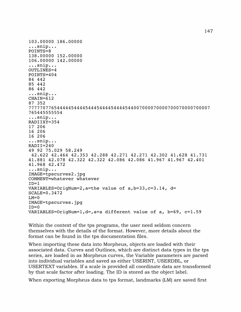
147
103.00000 186.00000...snip...POINTS=8138.00000 152.00000106.00000 142.00000...snip...OUTLINES=4POINTS=40484 44285 44286 442...snip...CHAIN=61287 3527777707765444445444454445444454444544007000070000700070000700007765445555554...snip...RADIIXY=35417 20616 20616 206...snip...RADII=24049 92 75.029 58.249 42.622 42.464 42.353 42.288 42.271 42.271 42.302 41.628 41.731 41.881 42.078 42.322 42.322 42.086 42.086 41.967 41.967 42.401 41.968 42.472...snip...IMAGE=tpscurves2.jpgCOMMENT=whatever whateverID=1 VARIABLES=OrigNum=2,a=the value of a,b=33,c=3.14, d= SCALE=0.3472LM=0IMAGE=tpscurves.jpgID=0 VARIABLES=OrigNum=1,d=,a=a different value of a, b=69, c=1.59
Within the context of the tps programs, the user need seldom concern themselves with the details of the format. However, more details about the format can be found in the tps documentation files.
When importing these data into Morpheus, objects are loaded with their associated data. Curves and Outlines, which are distinct data types in the tps series, are loaded in as Morpheus curves, the Variable parameters are parsed into individual variables and saved as either USERINT, USERDBL, or USERTEXT variables. If a scale is provided all coordinate data are transformed by that scale factor after loading. The ID is stored as the object label.
When exporting Morpheus data to tps format, landmarks (LM) are saved first
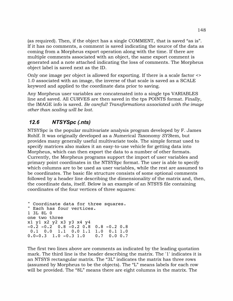
148
(as required). Then, if the object has a single COMMENT, that is saved “as is”. If it has no comments, a comment is saved indicating the source of the data as coming from a Morpheus export operation along with the time. If there are multiple comments associated with an object, the same export comment is generated and a note attached indicating the loss of comments. The Morpheus object label is saved next as the ID.
Only one image per object is allowed for exporting. If there is a scale factor <> 1.0 associated with an image, the inverse of that scale is saved as a SCALE keyword and applied to the coordinate data prior to saving.
Any Morpheus user variables are concatenated into a single tps VARIABLES line and saved. All CURVES are then saved in the tps POINTS format. Finally, the IMAGE info is saved. Be careful! Transformations associated with the image other than scaling will be lost.
12.6 NTSYSpc (.nts)NTSYSpc is the popular multivariate analysis program developed by F. James Rohlf. It was originally developed as a Numerical Taxonomy SYStem, but provides many generally useful multivariate tools. The simple format used to specify matrices also makes it an easy-to-use vehicle for getting data into Morpheus, which can then export the data to a number of other formats. Currently, the Morpheus programs support the import of user variables and primary point coordinates in the NTSYSpc format. The user is able to specify which columns are to be used as user variables, while the rest are assumed to be coordinates. The basic file structure consists of some optional comments followed by a header line describing the dimensionality of the matrix and, then, the coordinate data, itself. Below is an example of an NTSYS file containing coordinates of the four vertices of three squares:
" Coordinate data for three squares." Each has four vertices.1 3L 8L 0one two threex1 y1 x2 y2 x3 y3 x4 y4 -0.2 -0.2 0.8 -0.2 0.8 0.8 -0.2 0.8 0.1 0.0 1.1 0.0 1.1 1.0 0.1 1.00.0-0.3 1.0 -0.3 1.0 0.7 0.0 0.7
The first two lines above are comments as indicated by the leading quotation mark. The third line is the header describing the matrix. The '1' indicates it is an NTSYS rectangular matrix. The “3L” indicates the matrix has three rows (assumed by Morpheus to be the objects). The “L” means labels for each row will be provided. The “8L” means there are eight columns in the matrix. The
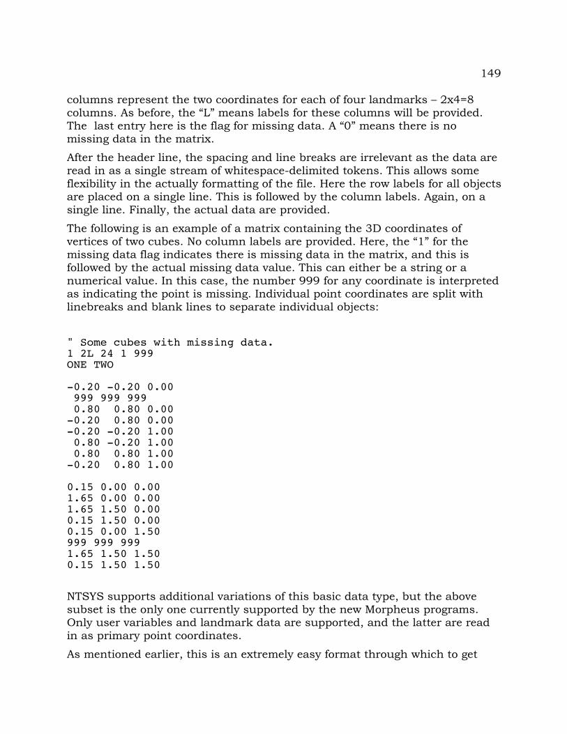
149
columns represent the two coordinates for each of four landmarks – 2x4=8 columns. As before, the “L” means labels for these columns will be provided. The last entry here is the flag for missing data. A “0” means there is no missing data in the matrix.
After the header line, the spacing and line breaks are irrelevant as the data are read in as a single stream of whitespace-delimited tokens. This allows some flexibility in the actually formatting of the file. Here the row labels for all objects are placed on a single line. This is followed by the column labels. Again, on a single line. Finally, the actual data are provided.
The following is an example of a matrix containing the 3D coordinates of vertices of two cubes. No column labels are provided. Here, the “1” for the missing data flag indicates there is missing data in the matrix, and this is followed by the actual missing data value. This can either be a string or a numerical value. In this case, the number 999 for any coordinate is interpreted as indicating the point is missing. Individual point coordinates are split with linebreaks and blank lines to separate individual objects:
" Some cubes with missing data.1 2L 24 1 999ONE TWO
-0.20 -0.20 0.00 999 999 999 0.80 0.80 0.00-0.20 0.80 0.00-0.20 -0.20 1.00 0.80 -0.20 1.00 0.80 0.80 1.00-0.20 0.80 1.00
0.15 0.00 0.001.65 0.00 0.001.65 1.50 0.000.15 1.50 0.000.15 0.00 1.50999 999 9991.65 1.50 1.500.15 1.50 1.50
NTSYS supports additional variations of this basic data type, but the above subset is the only one currently supported by the new Morpheus programs. Only user variables and landmark data are supported, and the latter are read in as primary point coordinates.
As mentioned earlier, this is an extremely easy format through which to get

150
new data into Morpheus. One need only cut-and-paste coordinate data for individuals into an ASCII text file and add the appropriate header as described above.
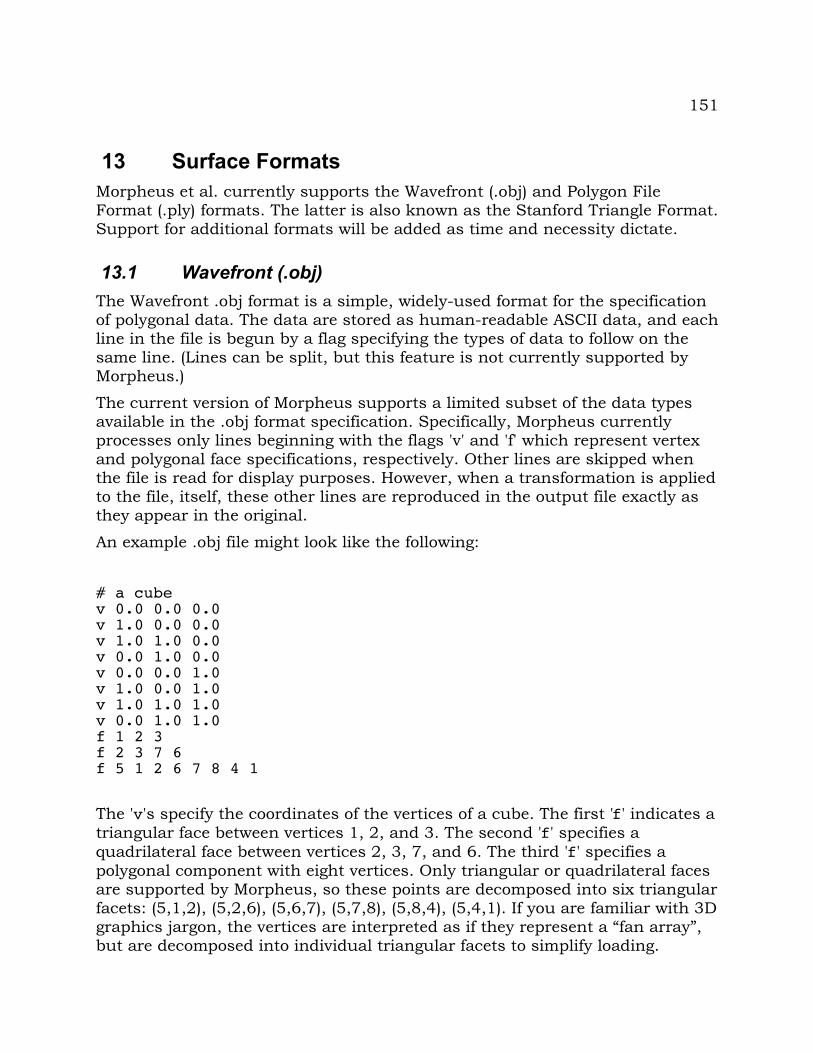
151
13 Surface FormatsMorpheus et al. currently supports the Wavefront (.obj) and Polygon File Format (.ply) formats. The latter is also known as the Stanford Triangle Format. Support for additional formats will be added as time and necessity dictate.
13.1 Wavefront (.obj)The Wavefront .obj format is a simple, widely-used format for the specification of polygonal data. The data are stored as human-readable ASCII data, and each line in the file is begun by a flag specifying the types of data to follow on the same line. (Lines can be split, but this feature is not currently supported by Morpheus.)
The current version of Morpheus supports a limited subset of the data types available in the .obj format specification. Specifically, Morpheus currently processes only lines beginning with the flags 'v' and 'f' which represent vertex and polygonal face specifications, respectively. Other lines are skipped when the file is read for display purposes. However, when a transformation is applied to the file, itself, these other lines are reproduced in the output file exactly as they appear in the original.
An example .obj file might look like the following:
# a cubev 0.0 0.0 0.0v 1.0 0.0 0.0v 1.0 1.0 0.0v 0.0 1.0 0.0v 0.0 0.0 1.0v 1.0 0.0 1.0v 1.0 1.0 1.0v 0.0 1.0 1.0f 1 2 3f 2 3 7 6 f 5 1 2 6 7 8 4 1
The 'v's specify the coordinates of the vertices of a cube. The first 'f' indicates a triangular face between vertices 1, 2, and 3. The second 'f' specifies a quadrilateral face between vertices 2, 3, 7, and 6. The third 'f' specifies a polygonal component with eight vertices. Only triangular or quadrilateral faces are supported by Morpheus, so these points are decomposed into six triangular facets: (5,1,2), (5,2,6), (5,6,7), (5,7,8), (5,8,4), (5,4,1). If you are familiar with 3D graphics jargon, the vertices are interpreted as if they represent a “fan array”, but are decomposed into individual triangular facets to simplify loading.
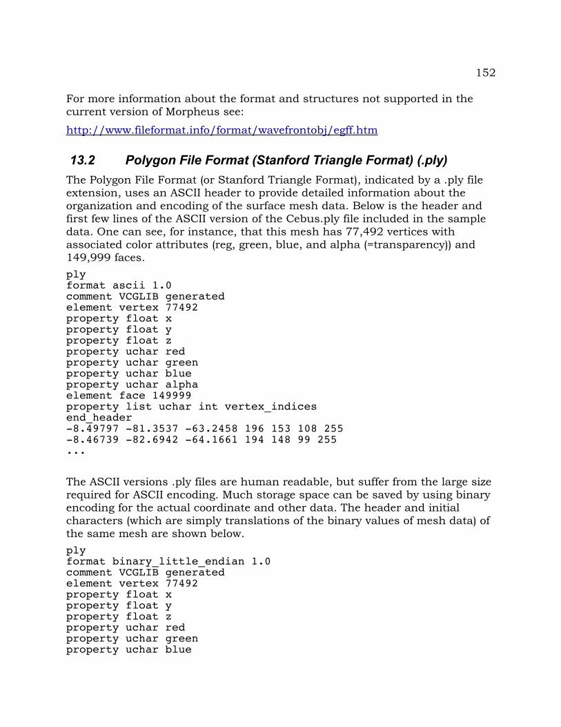
152
For more information about the format and structures not supported in the current version of Morpheus see:
http://www.fileformat.info/format/wavefrontobj/egff.htm
13.2 Polygon File Format (Stanford Triangle Format) (.ply)The Polygon File Format (or Stanford Triangle Format), indicated by a .ply file extension, uses an ASCII header to provide detailed information about the organization and encoding of the surface mesh data. Below is the header and first few lines of the ASCII version of the Cebus.ply file included in the sample data. One can see, for instance, that this mesh has 77,492 vertices with associated color attributes (reg, green, blue, and alpha (=transparency)) and 149,999 faces.plyformat ascii 1.0comment VCGLIB generatedelement vertex 77492property float xproperty float yproperty float zproperty uchar redproperty uchar greenproperty uchar blueproperty uchar alphaelement face 149999property list uchar int vertex_indicesend_header-8.49797 -81.3537 -63.2458 196 153 108 255 -8.46739 -82.6942 -64.1661 194 148 99 255 ...
The ASCII versions .ply files are human readable, but suffer from the large size required for ASCII encoding. Much storage space can be saved by using binary encoding for the actual coordinate and other data. The header and initial characters (which are simply translations of the binary values of mesh data) of the same mesh are shown below. plyformat binary_little_endian 1.0comment VCGLIB generatedelement vertex 77492property float xproperty float yproperty float zproperty uchar redproperty uchar greenproperty uchar blue

153
property uchar alphaelement face 149999property list uchar int vertex_indicesend_header¨˜#¡#µ¢¬ß˚|¬ƒôlˇlz#¡lc•¬...
The binary example is from the actual file distributed with Morpheus et al. By comparison, this version takes up around 3 megabytes of storage, while the ASCII version requires over twice that amount. The .ply files distributed with Morpheus are of relatively reduced resolution. The space savings of binary encoding becomes even more apparent with higher-resolution files. For example, one file with 1.3 million vertices and 2.6 million faces without color is 110 megabytes in size with ASCII encoding and 51.3 megabytes with binary encoding.