monte carlo tree search and alphago - yisong yue · advantages/disadvantages of mcts aheuristic no...

Monte Carlo Tree Search and AlphaGo

Suraj Nair, Peter Kundzicz, Kevin An, Vansh Kumar

Zero-Sum Games and AI● A player’s utility gain or loss is exactly balanced by the combined gain or loss

of opponents:○ E.g. - Given a pizza with 8 slices to share between person A and B.

■ A eats 1 slice.● A experiences +1 net utility.● B experiences -1 net utility.

● This is a powerful concept important to AI development for measuring the cost/benefit of a particular move.

● Nash Equilibrium.

Games and AI

● Traditional strategy - Minimax:○ Attempt to minimize opponent’s

maximum reward at each state (Nash Equilibrium)

○ Exhaustive Search

Player 1

Player 2

Player 1

Player 2

Drawbacks● The number of moves to be

analyzed quickly increases in depth.● The computation power limits how

deep the algorithm can go.Player 1

Player 2

Player 1

Player 2

Alternative Idea● Bandit-Based Methods

○ Choosing between K actions/moves.

○ Need to maximize the cumulative reward by continuously picking the best move.

● Given a game state we can treat each possible move as an action.

● Some problems / Further improvements:

○ Once we pick a move the state of the game changes.

○ The true reward of each move depends on subsequently possible moves.

Player 1

Player 2

Player 1

Player 2

Monte Carlo Tree Search ● Application of the Bandit-Based Method.● Two Fundamental Concepts:

○ The true value of any action can be approximated by running several random simulations.

○ These values can be efficiently used to adjust the policy (strategy) towards a best-first strategy.

● Builds a partial game tree before each move. Then selection is made.○ Moves are explored and values are updated/estimated.

General Applications of Monte Carlo Methods● Numerical Algorithms● AI Games

○ Particularly games with imperfect information○ Scrabble/Bridge○ Also very successful in Go (We will hear more about this later)

● Many other applications○ Real World Planning○ Optimization○ Control Systems

Understanding Monte Carlo Tree Search

MCTS Overview

● Iteratively building partial search tree● Iteration

○ Most urgent node■ Tree policy■ Exploration/exploitation

○ Simulation■ Add child node■ Default policy

○ Update weights

Development of MCTS● Kocsis and Szepesvári, 2006

○ Formally describing bandit-based method○ Simulate to approximate reward

● Proved MCTS converges to minimax solution● UCB1: finds optimal arm of upper confidence bound (UCT employed UCB1

algorithm on each explored node)

Algorithm Overview

Policies● Policies are crucial for how MCTS operates● Tree policy

○ Used to determine how children are selected

● Default policy○ Used to determine how simulations are run (ex. randomized)○ Result of simulation used to update values

Selection● Start at root node● Based on Tree Policy select child● Apply recursively - descend through tree

○ Stop when expandable node is reached○ Expandable -

■ Node that is non-terminal and has unexplored children

Expansion● Add one or more child nodes to tree

○ Depends on what actions are available for the current position○ Method in which this is done depends on Tree Policy

Simulation● Runs simulation of path that was selected● Get position at end of simulation● Default Policy determines how simulation is run● Board outcome determines value

Backpropagation● Moves backward through saved path● Value of Node

○ representative of benefit of going down that path from parent

● Values are updated dependent on board outcome○ Based on how the simulated game ends, values are updated

Policies● Tree policy

○ Select/create leaf node○ Selection and Expansion○ Bandit problem!

● Default policy○ Play the game till end○ Simulation

● Selecting the best child○ Max (highest weight)○ Robust (most visits)○ Max-robust (both, iterate if none exists)

UCT Algorithm● Selecting Child Node - Multi-Arm Bandit Problem● UCB1 for each child selection● UCT -

● n - number of times current(parent) node has been visited● nj - number of times child j has been visited● Cp - some constant > 0● Xj - mean reward of selecting this position

○ [0, 1]

UCT Algorithm

● nj = 0 means infinite weight○ Guarantees we explore each child node at least once

● Each child has non-zero probability of selection● Adjust Cp to change exploration vs exploitation tradeoff

Advantages/disadvantages of MCTS● Aheuristic

○ No need for domain-specific knowledge○ Other algos may work better if heuristics exists

■ Minimax for Chess

■ Better because chess has strong heuristics that can decrease size of tree.

● Anytime○ Can stop running MCTS at any time○ Return best action

● Asymmetric○ Favor more promising nodes

● Ramanujan et al.○ Trap states = UCT performs worse

○ Can’t model sacrifices well (Queen Sacrifice in Chess)

Example - Othello

Rules of Othello ● Alternating turns● You can only make a move that sandwiches a

continuous line of your opponent's pieces between yours○ Color of sandwiched pieces switches to your color

● Ends when board is full● Winner is whoever has more pieces

Example - The Game of Othello

root

m4m3m2m1m1

m2

m3

m4

● nj - initially 0○ all weights are initially infinity

● n - initially 0● Cp - some constant > 0

○ For this example ○ C = (1 / 2√2)

● Xj - mean reward of selecting this position

○ [0, 1]○ Initially N/A

Example - The Game of Othello cont.

root

m4m3m2m1

Xj n nj

m1 1 4 1

m2 1 4 1

m3 1 4 1

m4 0 4 1

m1

m2

m3

m4

After first 4 iterations: Suppose m1, m2, m3 black wins in simulation and m4 white wins

(Xj, n, nj) - (Mean Value, Parent Visits, Child Visits)

Example - The Game of Othello Iter #5root

m4m3m2m1m1m11

m12

m13

m13m12m11


(0, 4, 1)(1, 4, 1)(1, 4, 1)(1, 4, 1)

(N/A, 1, 0) (N/A, 1, 0) (N/A, 1, 0)

● First selection picks m1● Second selection picks m11

Black’s Move

White’s Move


m4m3m2m1m1

m11

(0, 5, 1)(1, 5, 1)(1, 5, 1)(.5, 5, 2)

(1, 2, 1)

● Run a simulation● White Wins● Backtrack, and update mean scores

accordingly.

Black’s Move

White’s Move



m4m3m2m1

m11

(0, 5, 1)(1, 5, 1)(1, 5, 1)(.5, 5, 2)

(1, 2, 1)

1.3972.269

2.269

1.269

● Suppose we first select m2

Black’s Move

White’s Move



m4m3m2m1

(0, 5, 1)(1, 5, 1)(1, 5, 1)(.5, 5, 2)

1.3972.269

2.269

1.269

m23m22m21(N/A, 1, 0) (N/A, 1, 0) (N/A, 1, 0)

● Suppose we pick m22

m23

m21 m22

White’s Move

Black’s Move


m11(1, 2, 1)


m4m3m2m1

(0, 6, 1)(1, 6, 1)(1, 6, 2)(.5, 6, 2)

m22(0, 2, 1)

● Run simulated game from this position.● Suppose black wins the simulated game.● Backtrack and update values

Black’s Move


m11(1, 2, 1)

White’s Move


m4m3m2m1

(1, 6, 2)(.5, 6, 2)

m23m22m21(N/A, 2, 0) (0, 2, 1) (N/A, 2, 0)

White’s Move

Black’s Move

m13m11(1, 2, 1) (N/A, 2, 0)

1.4472.339

1.339

(1, 6, 1) (0, 6, 1)

1.947

∞ ∞ ∞1.833

0.833

● This is how our tree looks after 6 iterations.● Red Nodes not actually in tree ● Now given a tree, actual moves can be made using max, robust, max-

robust, or other child selection policies.● Only care about subtree after moves have been made


∞

m12(N/A, 2, 0)

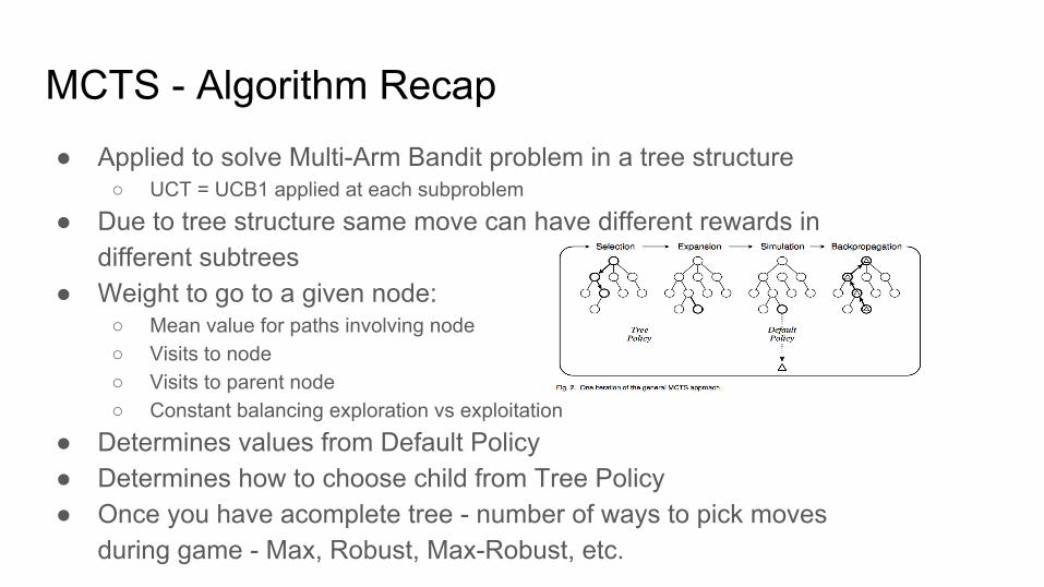
MCTS - Algorithm Recap● Applied to solve Multi-Arm Bandit problem in a tree structure

○ UCT = UCB1 applied at each subproblem

● Due to tree structure same move can have different rewards in different subtrees

● Weight to go to a given node:○ Mean value for paths involving node○ Visits to node○ Visits to parent node○ Constant balancing exploration vs exploitation

● Determines values from Default Policy● Determines how to choose child from Tree Policy● Once you have acomplete tree - number of ways to pick moves

during game - Max, Robust, Max-Robust, etc.

Analysis of UCT Algorithm

UCT Algorithm Convergence

● UCT is an application of the bandit algorithm (UCB1) for Monte Carlo search● In the case of Go, the estimate of the payoffs is non-stationary (mean payoff

of move shifts as games are played)● Vanilla MCTS has not been shown to converge to the optimal move (even

when iterated for a long period of time) for non-stationary bandit problems● UCT Algorithm does converge to optimal move at a polynomial rate at the root

of a search tree with non-stationary bandit problems● Assumes that the expected value of partial averages converges to some

value, and that the probability that experienced average payoff is a factor off of the expected average is less than delta if we play long enough


● Builds on earlier work by Auer (2002) who proved UCB1 algorithm converged for stationary distributions

● Since UCT algorithm views each visited node as running a separate UCB1 algorithm, bounds are made on expected number of plays on suboptimal arms, pseudo-regret measure, deviation from mean bounds, and eventually proving that UCB1 algorithm plays an suboptimal arm with 0 probability giving enough time

● Kocsis and Szepesvári’s work was very similar, with additions of ε-δ type arguments using the convergence of payoff drift to remove the effects of drift in their arguments, especially important in their regret upper bounds


● After showing UCB1 correctly converges to the optimal arm, the convergence of UCT follows with an induction argument on search tree depth

● For a tree of depth D, we can consider the all children of the root node and their associated subtrees.

● Induction hypothesis gives probability of playing suboptimal arm goes to 0 (base case is just UCB1), and the pseudo-regret bounds and deviation from partial mean bounds ensures the drift is accounted for

● The most important takeaway is when a problem can be rephrased in terms of multi-armed bandits (even with drifting average payoff), similar steps can be used to show failure probability goes to 0

Variations to MCTSApplying MCTS to different game domains

Go and other Games● Go is a combinatorial game.

○ Zero-sum, perfect information, deterministic, discrete and sequential.

● What happens when some of these aspects of the game change?

Multi-player MCTS● The central principle of minimax search:

○ The searching player seeks to find the move to maximize their reward while their opponent seeks to minimize it.

○ In the case of two players: each player seeks to maximize their own reward.

● Not necessarily true in the case of more than two players.○ Is the loss of player 1 and gain of player 2 necessarily a gain for player 3?

Multi-player MCTS● More than 2 players does not guarantee zero-sum game.● No perfect way to model reward/loss among all players● Simple suggestion - maxn idea:

○ Nodes store a vector of rewards.○ UCB then seeks to maximize the value using the appropriate vector component depending.○ Components of vector used depend on the current player.○ But how exactly are these components combined?

MCTS in Multi-player Go● Cazenave applies several variants of UCT to Multi-player Go.

○ Because players can have common enemies he considers the possibility of “coalitions”

● Uses maxn, but takes into account the moves that may be adversarial towards coalition members.

● Changes scoring to include the coalition stones as if they were the player’s own.

MCTS in Multi-player Go● Different ways to treat coalitions:

○ Paranoid UCT: player assumes all other players are in coalition against him.■ Coalition Reduction■ Usually better than Confident.

○ Confident UCT: searches are completed with the possibility of coalition with each other one player. Move is selected based on whichever coalition could prove most beneficial.

■ Better when algorithms of other players are known.○ Etc.

● No known perfect way to model strategy equilibrium between more than two players.

Variation Takeaway● Game Properties:

○ Zero-sum: Reward across all players sums to zero.○ Information: Fully or partially observable to the players.○ Determinism: Chance Factors?○ Sequential/Simultaneous actions.○ Discrete: Whether actions are discrete or applied in real-time.

● MCTS is altered in order to apply to different games not necessarily combinatorial.

AlphaGo

Go● 2 player● Zero-sum● 19x19 board● Very large search tree

○ Breadth ≈ 250, depth ≈ 150○ Unlike chess

● No amazing heuristics○ Human intuition hard to replicate

● Great candidate for applying MCTS○ Vanilla MCTS not good enough

How to make MCTS work for Go?Idea 1: Value function to truncate tree -> shallower MCTS search

Idea 2: Better tree & default policies -> smarter MCTS search

● Value function○ Expected future reward from board s assuming we play perfectly from that point

● Tree policy○ Selecting which part of the search tree to expand

● Default policy○ Determine how simulations are run○ Ideally, should be perfect player

Before AlphaGo● Strongest programs

○ MCTS○ Enhanced by policies predicting expert moves

■ Narrow search tree○ Limitations

■ Simple heuristics from expert players■ Value functions based on linear combinations of input features

○ Cannot capture full breadth of human intuition○ Generally only looking a few moves ahead○ Local v global approach to reward

AlphaGo - Training● AlphaGo

○ Uses both ideas for improving MCTS○ Two resources

■ Expert data■ Simulator (self-play)

○ Value function■ Expected future reward from a board s assuming we play perfectly from that point

○ Tree & Default Policy networks■ Probability distributions over possible moves a from a board s■ Distribution encodes reward estimates

Main idea: For better policies and value functions, train with deep convolutional networks

AlphaGo - Training

Human expert positions Self-play positions

Rollout policy SL policy network RL policy network Value function

AlphaGo - Training● Supervised Learning network pσ

○ Slow to evaluate○ Goal = predict expert moves well, prior probabilities for each move

● Fast rollout network pπ○ Default policy○ Goal = quick simulation/evaluation

● Reinforcement Learning network pρ○ Play games between current network and randomly selected previous iteration○ Goal = optimize on game play, not just predicting experts

● Value function vP(s)○ Self-play according to optimal policies pr for both players from pρ○ Default policy○ Function of a board, not probability distribution of moves○ Goal = get expected future reward assuming our best estimate of perfect play

AlphaGo - Playing● Each move

○ Time constraint○ Deepen/build our MCTS search tree○ Select our optimal move and only consider subtree from there

● at - action selected at time step t from board st● Q(st, a) - average reward for playing this move (exploitation term)● P(s, a) - prior expert probability of playing moving a● N(s, a) - number of times we have visited parent node● u acts as a bonus value

○ Decays with repeated visits

AlphaGo - Playing (Selection/Tree Policy)

AlphaGo - Playing (Policy Recap)

Human expert positions Self-play positions

Rollout policy SL policy network RL policy network Value function

● When leaf node is reached, it has a chance to be expanded● Processed once by SL policy network (pσ) and stored as prior probs P(s, a)● Pick child node with highest prior prob

AlphaGo - Playing (Expansion)

● Default policy, of sorts● vθ - value from value function of board position sL● zL - Reward from fast rollout p

○ Played until terminal step

● λ - mixing parameter○ Empirical

AlphaGo - Playing (Evaluation/Default Policy)

● Extra index i is to denote the ith simulation, n total simulations● Update visit count and mean reward of simulations passing through node● Once search completes:

○ Algorithm chooses the most visited move from the root position

AlphaGo - Playing (Backup)

AlphaGo Results

AlphaGo Takeaway

● You should work for Google

● Tweaks to MCTS are not independently novel● Deep learning allows us to train good policy networks● Have data and computation power for deep learning

○ Can now solve a huge game such as Go

● Method applicable to other 2 player zero-sum games as well

Questions?

monte carlo tree search and alphago - yisong yue · advantages/disadvantages of mcts aheuristic no...

Documents