monte carlo state-space likelihoods by weighted posterior...

Monte Carlo State-Space Likelihoods by WeightedPosterior Kernel Density Estimation

Perry DE VALPINE

Maximum likelihood estimation and likelihood ratio tests for nonlinear non-Gaussian state-space models require numerical integration forlikelihood calculations Several methods including Monte Carlo (MC) expectation maximization MC likelihood ratios direct MC integra-tion and particle lter likelihoods are inef cient for the motivating problem of stage-structured population dynamics models in experimen-tal settings An MC kernel likelihood (MCKL) method is presented that estimates classical likelihoods up to a constant by weighted kerneldensity estimates of Bayesian posteriors MCKL is derived by using Bayesian posteriors as importance sampling densities for unnormalizedkernel smoothing integrals MC error and mode bias due to kernel smoothing are discussed and two methods for reducing mode bias areproposed ldquozooming inrdquo on the maximum likelihood parameters using a focused prior based on an initial estimate and using a posteriorcumulant-based approximation of mode bias A simulated example shows that MCKL can be much more ef cient than previous approachesfor the population dynamics problem The zooming-in and cumulant-based corrections are illustrated with a multivariate variance estimationproblem for which accurate results are obtained even in 20 parameter dimensions

KEY WORDS Importance sampling Monte Carlo expectation maximization Monte Carlo kernel likelihood Monte Carlo likelihoodratio Population dynamics State-space model

1 INTRODUCTION

A dif culty for frequentist likelihood-based analysis withmechanistic models is that the models often include unknownstates or process errors so that likelihood calculations requirehigh-dimensional integrations Approaches to maximum like-lihood estimation using Monte Carlo (MC) integration in thissetting include MC expectation maximization (MCEM) (Weiand Tanner 1990 Chan and Ledolter 1995 McCulloch 1997Robert and Casella 1999 Booth and Hobert 1999 Huumlrzelerand Kuumlnsch 2001 Levine and Casella 2001) MC likelihoodratio (MCLR) estimation via importance sampling (Geyer andThompson 1992 Geyer 1994 1996 McCulloch 1997) basicMC integrationmore advanced MC integrationsuch as impor-tance sampling (Durbin and Koopman 1997 2000) and parti-cle ltering (PF) (Gordon Salmond and Smith 1993Kitagawa1996 1998 Pitt and Shephard 1999 Doucet de Freitas andGordon 2001b Huumlrzeler and Kuumlnsch 2001) However for mymotivating model a biologically stage-structured populationdynamics model for a replicated experimental setting none ofthese methods is very ef cient

I present a faster approach based on estimating likelihoodsfrom weighted kernel density estimates of a Bayesian poste-rior which is motivated by importance sampling the kernelsmoothing integral I consider convergence and accuracy ofthe method including MC error and mode bias due to ker-nel smoothing I give methods to gain accuracy by ldquozoominginrdquo on the likelihood maximum using focused priors whichis equivalent to importance sampling near the maximum andto estimate the mode bias due to kernel smoothing using pos-terior cumulants I give a second example showing that evenin 10ndash20 dimensions these methods can provide high accu-racy for chi-squared hypothesis test cutoffs This approach maybe widely and easily applicable because it can take advan-tage of the boom in computational methods for Bayesian pos-terior sampling

Perry de Valpine is Postdoctoral Researcher Department of Integra-tive Biology University of California Berkeley CA 94720-3140 (E-maildevalpinnceasucsbedu) This work was supported by the National Centerfor Ecological Analysis and Synthesis a center funded by the National Sci-ence Foundation (grant DEB-0072909) the University of California (UC) andUC Santa Barbara and the US Department of Agriculture National ResearchInitiative Competitive Grants Program

My investigation is motivated by the need to t demographicmodels to time series from ecological population dynamicsexperiments In population ecology there is a wide gap be-tween plausible mechanistic models and models commonlyused to analyze data Population dynamics experiments typi-cally produce replicated time series structured by species lifestages within species andor location These common typesof experiments (reviewed by Hairston 1989 Underwood 1997Resetarits and Bernardo 1998) follow a long tradition that in-cludes classic work by Huffaker (1958) on predatory and her-bivorous spider mites and by Gause (1934) and Luckinbill(1973) on predator and prey protozoans Population dynamicsexperiments are used to study direct and indirect species inter-actions (eg Wootton 1994 Rosenheim Kaya Ehler Maroisand Jaffee 1995 Karban English-Loeb and Hougen-Eitzman1997 MurdochNisbet McCauley de Roos and Gurney 1998Ellner et al 2001 Rosenheim 2001 Snyder and Ives 2001)population cycles (eg Nicholson and Bailey 1935 GurneyBlythe and Nisbet 1980McCauleyNisbet Murdoch de Roosand Gurney 1999) speciesrsquo roles in ecosystem functioning(eg Naeem Thompson Lawler Lawton and Wood n 1994Downing and Leibold 2002) trophic cascades (eg Carpenterand Kitchell 1993 Ives Carpenter and Dennis 1999 StrongWhipple Child and Dennis 1999 Pace Cole Carpenter andKitchell 1999 Klug Fischer Ives and Dennis 2000) and labo-ratory ldquomodelrdquo systems (eg Costantino Desharnais Cushingand Dennis 1997 Kaunzinger and Morin 1998 Holyoak 2000Dennis Desharnais Cushing Henson and Costantino 2001)

I use agricultural insect ecology to illustrate the model- ttingproblem for population dynamics experiments Entomologistsroutinelyconduct laboratorygreenhouse and eld experimentsin which abundancesof eggs immatures and adults of differentspecies are estimated at several times under variousplant condi-tions predator communities or other experimental treatmentsCurrently such data are almost always analyzed with general-ized linear models that do not re ect processes of reproduc-tion growth mortality and predation that produced the dataIn contrast the models used for theoreticalstudies of population

copy 2004 American Statistical AssociationJournal of the American Statistical Association

June 2004 Vol 99 No 466 Theory and MethodsDOI 101198016214504000000476

523

524 Journal of the American Statistical Association June 2004

dynamics describe these processes and often involve nonlinearpredatorndashprey interactions time lags arising from developmentand other factors that can produce complex dynamics (egMetz and Diekmann 1986 Tuljapurkar and Caswell 1997Gurney and Nisbet 1998)

Because of their relative dimensionalityof noises states ob-servations and replicates experimental population dynamicsproblemshave a different balance of ef ciency issues than otherstate-space or hidden-variables problems MC state-space re-search has typically considered methods for single long timeseries such as for nancial data (Carlin Polson and Stoffer1992 Shephard and Pitt 1997 Tanizaki and Mariano 1998Pitt and Shephard 1999 Durham and Gallant 2002) or sh-eries catch and survey records (Bjoslashrnstad Fromentin Stensethand Gjosaeter 1999 Meyer and Millar 1999 Millar and Meyer2000) At the other extreme MC methods for experimentaldatahave been applied to generalized linear mixed models wheredata are iid and the likelihood requires a MC integration overunknown random variables (Clayton 1996 McCulloch 1997Booth and Hobert 1999) Experimental population dynamicsdata mix these features in the form of short replicated time se-ries In addition realistic populationdynamics models are oftencontinuous in time or have a short time step so that the spaceof random disturbances entering the process may be of muchhigher dimension than the observationspace Also the aim hereis to calculate approximate likelihood ratio tests whereas mostMC state-space research has addressed nonexperimental set-tings with more focus on ltering and smoothing than on pa-rameter estimation and testing

I compare ve MC methods for likelihood maximizationTwo of the main approaches in the literature are MCEM (Weiand Tanner 1990 Chan and Ledolter 1995 McCulloch 1997Robert and Casella 1999 Booth and Hobert 1999) and MCLR(Geyer and Thompson 1992 Geyer 1994 1996 McCulloch1997) which both use alternating steps of MC sampling andlocal maximization (but see Levine and Casella 2001 for po-tential improvements) Two other natural candidates for theproblem are PF (Gordon et al 1993 Kitagawa 1996 Pitt andShephard 1999 Doucet et al 2001b) and basic MC integra-tion possibly with importance sampling which I call MC di-rect (MCD) The method developedhere MC kernel likelihood(MCKL) temporarily treats parameters as random variablesfor purposes of Markov Chain MC (MCMC) sampling andthen uses a weighted kernel density estimator to approximatea classical likelihood surface MCKL is related to kernel den-sity estimation of Bayesian posterior distributions (West 1993Chen 1994 Givens and Raftery 1996 Liu and West 2001) butthe approach here of using kernel density estimates to recoverthe classical likelihood surface for a state-space model appearsto be new

Next I introduce the MC likelihood methods in detailFor MCKL I discuss convergence MC error and smoothingmode bias zooming in by resampling near the mode to reducesmoothing bias and estimating smoothing bias from posteriorcumulants I then introduce an example population model andhypothetical experiment and compare maximum likelihoodconvergence of the different methods Finally I use a problemof multivariate standard deviation estimation to illustrate andevaluate the zooming and cumulant-basedcorrections

2 MONTE CARLO LIKELIHOOD METHODS

Suppose that there are n experimental units with data vec-tors Yi i D 1 n which include both multiple times andmultiple observation dimensions To be more explicit denoteYi D Yi1 YiT where Yit is a vector of observa-tions at time t and there is a xed set of observation timest D 1 T (For notational simplicity I assume the sameset of observation times for each replicate) The methods hererequire only that the model be amenable to various MC al-gorithms MCMC for the MCKL MCEM and MCLR meth-ods and sequential particle ltering for the PF method Foreach replicate i let ordm i be the unknown states or processnoises with probability density Prordm i and let PrYijordm i bethe probability density of observations given states Denoteordmi D ordm i1 ordm iT where ordm it are the process noisesfrom time t iexcl 1 to t which may include many model time steps(and noise values) between observation times

Each method aims to maximize the likelihood integral for thed-dimensional parameter vector 2

L2 DnY

iD1

ZPrYijordm iPrordm i dordm i (1)

or l2 D logL2 Although (1) makes sense with ordm as ei-ther states or process noises from here on I use it as processnoises and write Xordm for the states In other words PrYi jordm i

will usually involve a calculation of state dynamics from theprocess noises with the observation density related to the statevalues In the example that follows ordmrsquos are random environ-mental variations X is a time trajectory of dynamics for an agecohort model with a 1-day time step and Y is a time series ofestimates taken every 10 days of the abundance of several lifestages each of which is a summation of multiple age cohortsFor general introductionof each method I do not need to spec-ify dimensions for states noises or observations Treatment ofinitial conditions is assumed to be included in the notation Ifthese conditionsare xed then the state calculations start fromthem if they are random then they are included in the processnoises Dependence of probabilities on 2 is suppressed in thenotationFinally everything is written for continuousvariablesbut could be easily adapted to discrete variables

Only the MCD and PF methods estimate the likelihood with-out introducing an unknown constant For the other methodsafter estimating the maximum likelihood estimator (MLE) it isnecessary to estimate the likelihood at the MLE for purposesof likelihood ratio approximate hypothesis tests and I assumethat this is feasible For my populationdynamics example I dothis through an importance-sampled MC estimate of (1) withan estimate of each Prordm i jYi as the importance density foreach Prordm i (Shephard and Pitt 1997)

21 Monte Carlo Direct

The most obvious approach MCD draws a large sam-ple fordmj

i gmjD1 from each Prordm i and uses

l2 frac14nX

iD1

log

1m

mX

jD1

PriexclYi

shyshyordmj i

cent

(2)

This method suffers from the inef ciency of basic MC inte-gration a large variance of PrYi jordmj

i (Robert and Casella

de Valpine Monte Carlo State-Space Likelihoods 525

1999 sec 32) However it has the potential ef ciency that thesame noise sample and state trajectories can be used for eachreplicate within a treatment group If the same model appliesto i 2 I where I de nes a treatment group then a single sam-ple fordmj

I gmjD1 and only one calculation of each Xordm

j I can be

used in the inner sum of (2) for each i 2 I This may be usefulif Xordm

j i is the most computationallyintensive step for each j

For likelihood maximization MCD provides a smooth surfacein 2 if the same MC sample is used for all 2

22 Particle Filter

A basic PF or bootstrap lter (Doucet et al 2001a) like-lihood approximation uses a sampling importance-resampling(SIR)-type algorithm at each observation time to obtain a sam-ple from Prordm i jYi as follows The algorithm handles eachreplicate separately and subscripts i are omitted in this sectionand replaced with time subscripts Denote Yt D Yt ordm t D ordmtY1 t D Y1 Yt ordm1 t D ordm1 ordm t and ordm1 t j1 s Dordm1 t jY1 s Also de ne dummy variables Y0 D andY1 0 D Factor the likelihoodsequentially for each replicateso that

PrYj2 DTY

t D1

PrYt jY1 tiexcl1 (3)

PF uses the following steps starting with t D 1 and a sam-ple fordmj

1 t j1 tiexcl1gmj D1 from Prordm1 t j1 tiexcl1

1 Estimate PrYt jY1 tiexcl1 by direct MC integration as1m

PmjD1 PrYt jordmj

1 t j1 tiexcl1

2 De ne normalized weights wj D PrYt jordmj 1 t j1 tiexcl1=

PmjD1 PrYt jordmj

1 t j1 tiexcl13 Generate a sample from Prordm1 t j1 t by drawing

ordmj 1 t j1 tiexcl1 with probability wj

4 Generate a sample from Prordm1 tC1j1 t by drawing

ordmj tC1j1 t from Prordm tC1jordmj

1 t j1 t and setting ordmj 1 tC1j1 t D

ordmj 1 t j1 t ordm

j tC1j1 t Increment t and return to step 1

Gordon et al (1993) showed that this procedure works as-ymptotically (as m 1) but the primary dif culty in practiceis sample degradationas samples are lost in step 3 as t increases(Doucet et al 2001b) For likelihood maximization PF hasthe serious dif culty of not providing a smooth surface in 2Huumlrzeler and Kuumlnsch (2001) handled this by loess smoothingthe PF estimate of L2 a step that I do not try here becauseit would be computationallyexpensive in the dimensionalityofmy examples

23 Monte Carlo Expectation Maximization

MCEM works by using MC samples for the expectations ofthe EM algorithm The MCEM algorithm is to start with 20obtain samples fordmj

i gmjD1 from Prordm i jYi20 for each repli-

cate i nd 21 by maximizingnX

iD1

mX

jD1

1m

logPriexclYi ordm

j i

shyshy21cent

frac14nX

iD1

ZlogPrYiordm i j21 Prordm ijYi 20 dordm i (4)

and nally set 20 to the new value of 21 and repeat the pro-cedure The samples from Prordm i jYi 20 for each i could ingeneral be obtained with an MCMC or other algorithm Thismethod requires a sample for each replicate for each iterationof the algorithm althoughLevine and Casella (2001) suggestedsimply reweighting the previous sample according to impor-tance sampling principles if it covers the region of interest forthe next maximization step MCEM also has the advantagesand drawbacks of the EM algorithm (Chan and Ledolter 1995McCulloch 1997) it can be slow to converge and can convergeto local maxima

24 Monte Carlo Likelihood Ratio

MCLR works by using MC samples to approximate like-lihood ratios The approach is based on the importance sam-pling identity

l2 iexcl l2S

DnX

iD1

log

microZPrYi ordm ij2

PrYi ordm i j2SPrordm i jYi 2S dordm i

para (5)

For MC approximationone starts with a xed initial guess 2S

and obtains samples (like MCEM) fordmj i gm

jD1 from Prordm i jYi 2S for each replicate i and maximizes over 2

l2 iexcl l2S frac14nX

iD1

log

mX

jD1

PrYi ordmj i j2

PrYi ordmj i j2S

(6)

The ef ciency of this method depends on how the importancesampling approximation breaks down as 2 gets far from 2S and MCLR has been observed to perform poorly in somecases (Geyer 1994 McCulloch 1997) For example if 2 is thevariance of a normal distribution then for 2 gt 2S the MCapproximate integrals may not have nite variance (Robertand Casella 1999 sec 532) Geyer (1996) suggested iterat-ing the proceduremdashmaximize 2 in a trust region around 2S set 2S equal to 2 and start overmdashbut this does not neces-sarily solve the convergence issue Geyer (1994) and Geyer(1996) suggested using importance sampling distributions thatare mixtures of the conditional noise distributions from severaldifferent reference parameters This seems to work well for aone-dimensional parameter problem of an Ising model (Geyer1994) but would gain complexity for higher-dimensionalpara-meter spaces Like MCEM MCLR requires a sample for eachreplicate for each iteration of the algorithm

3 MONTE CARLO KERNEL LIKELIHOOD METHOD

The MCKL method appears to be a new approach to max-imum likelihood parameter estimation for state-space modelsbut it is related to kernel density estimation of Bayesian poste-rior densities (West 1993Chen 1994Givens and Raftery 1996Liu and West 2001)The approach involves temporarily treatingparameters as having probabilitydensities and sampling from aposterior density as in Bayesian methods The likelihood canthen be estimated up to a constant as a weighted kernel densityestimate with weights obtained by viewing the posterior as animportance sampling density (For a wide prior the likelihoodcan also be estimated up to a constant as an unweighted kernel


density estimate divided by the prior I brie y discuss this ver-sion later) MCKL does not involvea Bayesian interpretationofparameters because only likelihoods are recovered in the endbut I use terms like ldquopriorrdquo and ldquoposteriorrdquo for consistency withBayesian methods

MCKL involves the following steps

1 Choose a prior Pr2 and use an MCMC (or some otheralgorithm such as a joint parameter-state particle lterLiu and West 2001) to obtain a sample from

Pr2 ordm1 ordmnjY1 Yn

Pr2

nY

iD1

PrYiordm i j2 (7)

The 2 dimensions of this sample are a sample fromthe posterior

PrS2 acute Pr2jY1 Yn DL2Pr2

CS

DZ

cent cent centZ

Pr2ordm1 ordmnj

Y1 Yn dordm1 cent cent centdordmn (8)

where CS DR

L2Pr2 d22 Maximize the following kernel density estimate of the

likelihood up to the unknown constant CS

OLh2 D 1m

mX

jD1

Khiexcl2 2j

centwj (9)

wj D1

Pr2j

where f2j gmjD1 are the sample points and Kh is a

normalized kernel smoother function with multivariatebandwidth h D h1 hd For convenience I assumethroughout that Kh is orthogonal and oriented along thecoordinate axes that is Kh2 acute D

QdlD1 Khl

2l acutel

where hl 2l and acutel are the l-axis components of h2 and acute in d dimensions and Khl is a one-dimensionalkernel smoother For example for Gaussian Kh I usea diagonal covariance matrix with entries h2

1 h2d

I also assume Kh symmetric in every dimension withKh22j D Kh2 iexcl 2j

To see that (9) is an unnormalized importance-sampledkernel estimate of L consider a function g2 such thatR

g2L2 d2 exists The usual importance sampling mo-tivation isZ

g2L2 d2 DZ

g2L2

PrS2PrS2 d2 (10)

where PrS is an importance density MCKL uses the specialchoice PrS2 D Pr2L2=CS because L cannot be calcu-lated directly giving the MC estimate

Zg2L2 d2 frac14

CS

m

mX

jD1

g2j

Pr2j (11)

2j raquo PrS2 j D 1 m

MCKL uses g2j D Kh2 2j and drops the normaliza-tion constant CS

31 Convergence

Next I examine several aspects of MCKL convergence witha focus on understanding rather than technical proofs Romano(1988) proved almost sure convergence of modes of kernel es-timates as m 1 and h 0 with h Agrave logm=m (see alsoGrund and Hall 1995) These proofs have the useful feature ofrequiring regularity only in a neighborhoodof the true mode sothe possibilities of nonintegrabilityor in nite ldquomomentsrdquo of L

are not problematicSimply put in reasonable cases kernel den-sity estimates and their derivatives converge to their true valuesas m 1 and h 0 in a coordinated way so mode estimatesconverge to the true mode

To transfer proofs of convergence of kernel mode estimatesto the MCKL setting compare unweighted normalized ker-nel density estimates for which the proofs were developed tothe weighted unnormalizedkernel density estimates of MCKLThe relation between the unweighted and weighted estimatesis exactly the relation between simple MC integration andimportance-sampled MC integration and it is well known thatfor a well-chosen importance density the latter converges atleast as well as the former and is often more accurate The un-known normalizing constant of MCKL is bounded over properpriors (assuming bounded L) and scaling by a bounded con-stant also leaves proofs of mode convergenceintact Thus modeconvergence transfers to both the importance sampling andscaling aspects of MCKL Moreover MCKL can be more ac-curate for mode estimation in a region of high posterior densitythan unweightedkernel density estimates essentially because itcan use more sample points near the mode

32 Accuracy in Practice

As in kernel estimation of entire densities the key challengein kernel mode estimation is more practical than theoreticalmdashthat is to obtain useful choices of h gt 0 and m lt 1 Be-cause h gt 0 in practice it is useful to consider accuracy for xed h as m 1 Denote the true likelihood as L0 withtrue mode 20 and the smoothed likelihood as Lh D Kh curren L0where ldquocurrenrdquo denotes convolution with true mode 2h D 20 C12h and MCKL mode estimate O2h Here O2h iexcl 2h is the MCerror and 12h is the smoothing bias for xed h As beforeI use Kh orthogonal and oriented along the coordinate axeswith h D h1 hd I use the derivativenotation l D =2l lm D 2=2l2m and so on and rL D 1L dLr2Llm D lmL As m 1 CS

OLh Lh by the law of largenumbers In this setting I consider MC variance of the MCKLmode estimate as well as the more challenging problem of esti-mating and reducing its smoothing bias

33 Monte Carlo Variance

I use M-estimator theory (van der Vaart 1998) to describe theMC error The MCKL mode estimator O2h is a solution to theestimating equations

r OLh2 D 1m

mX

jD1

rKh2 iexcl 2j

Pr2j D 0 (12)


De ne Atildej 2 D Kh2 iexcl 2j =Pr2j General M-estima-tor theory gives that

pm O2h iexcl 2h is asymptotically normal

with mean 0 and variance

E[r2Atilde2h]iexcl1EpoundrAtilde2hrAtilde2hT

curren

pound E[r2Atilde2h]iexcl1 (13)

where expectations are with respect to PrS2 (van der Vaart1998 sec 53 using rAtilde instead of Atilde ) In terms of Lh

E[r2Atilde2h]iexcl1 D CS [r2Lh2h]iexcl1 (14)

and the l m matrix component of the middle expectation is

EpoundrAtilde2hrAtilde2hT

currenlm

D1

CS

Z[lKh2h iexcl 2][mKh2h iexcl 2]

Pr2L2 d2

(15)

These results require that E[r2Atilde2h] be invertible and non-trivially that (15) exist for all l m D 1 d (Use of m asa dimension subscript is separate from its use as sample sizethroughout)

When Pr2 and Kh are Gaussian with covariances 6Prand 6K (15) is nite when 26iexcl1

K iexcl 6iexcl1Pr is positive de -

nite which is always true for suf ciently small 6K When6Pr D diagfrac34 2

1 frac34 2d (ie 6Pr and 6K have the same eigen-

values) this amounts to h2l lt 2frac34 2

l for l D 1 d MC errorof O2h can be estimated by a plug-in estimator for (13) or bya bootstrap (for independent samples) or a moving-block boot-strap for sequentially-dependent samples such as from MCMC(Kunsch 1989 Efron and Tibshirani 1993 Mignani and Rosa1995) I now focus on the more dif cult problem of smooth-ing bias

34 Smoothing Bias

The usual conundrum of kernel density estimation is that es-timation of smoothing bias requires more accurate knowledgeof the density than is provided from the kernel estimates In thecurrent context this is revealed by approximating 12h forsmall h using the standard Taylor series for kernelestimates (Silverman 1986 Scott 1992 sec 63) Using2 D 21 2d 2h D 2h1 2hd Kh2 DQd

mD1Khm 2m Khm2m D K2m=hm=hm mKhm2m DK 02m=hm=h2

m and 12hm D 2hm iexcl 2m D hmtm allfor m D 1 d leads to

0 D lLh2h

DZ sup3 Y

m6Dl

Ktm

acuteK 0tl

hlL2h1 iexcl h1 t1 2hd iexcl hd td dt

(16)

Expanding L around 2h gives

0 DZ sup3 Y

m 6Dl

Ktm

acuteK 0tl

hl

poundmicro

L2h iexclX

i

hi ti iL2h C 1

2

X

ij

hihj ti tj ij L2h

iexcl 1

6

X

ijk

hihj hk ti tj tk ij kL2h C Oh4

paradt (17)

Integrating and expanding L around 20 relates 12h to h ForGaussian Kh this gives for each l

0 DdX

mD1

12hm lmL20

iexcldX

jD1

h2j

2

Aacute

ljjL20 CdX

mD1

12hm ljjmL20

C Oh4 (18)

Estimating 12h from (18) is useful only if the derivativesof L

are known with greater accuracy than the kernel estimates usedto estimate O2h in the rst place In the usual kernel densityestimation context with a xed data sample higher-order esti-mates are the primary option to reduce smoothing bias (Jonesand Signorini 1997) but these are ultimately limited by sam-ple size The MCKL situation is quite different because muchgreater improvements can be obtained by simulating additionalpoints in the region of the MLE which I consider next

341 Reducing Smoothing Bias by Zooming in Supposethat one has an initial estimate O2h using h m Pr2and PrS2 as well as some rough estimate of a new priorPr02 that will yield a new posterior Pr0

S2 with moreweight than PrS2 on 2h The following approximation ofthe MC error (13) shows that for suf ciently small h if Pr0

S2

puts more weight than PrS2 on 2h then it reduces (13)This implies that with a sample of size m from Pr0S an im-proved estimate O2h0 with h0

l lt hl l D 1 d can be ob-tained with smaller smoothing bias and no greater MC errorthan for O2h A natural choice for Pr0 is a parametric estimateof PrS which performs well in Example 2 of Section 5 Al-ternatively Pr0 might be based on an estimate of 12h whichcould come from a higher-order kernel estimate or for a wideprior from the cumulant-based estimate given below

De ne AS (with dependence on h implicit) to be the ma-trix factor of (13) that depends on Pr (or PrS ) that is AS

lm DC2

SE[rAtilde2hrAtilde2hT ]lm which from (15) is

ASlm D

Z[lKh2h iexcl y][mKh2h iexcl y]

Ly2

PrSydy (19)

Using the same type of expansion as (17) gives for the lth di-agonal element

ASll D

1

h2l

QdmD1 hm

poundmicro

L2h2

PrS2h[K]diexcl1[K 0]

C [K]diexcl2[K 0][K2]X

i 6Dl

h2i ii

sup3L2h2

PrS2h

acute

C [K]diexcl1[K 02]h

2l ll

sup3L2h2

PrS2h

acuteC Oh4

para (20)

where [K] DR

Kt2 dt [K 0] DR

K 0t2 dt [K2] DRt2Kt2 dt and [K 0

2] DR

t2K 0t2 dt Off diagonal-termscan be derived similarly but have no O1 term inside the


brackets For suf ciently small h the leading term indicatesthat asymptotic variance decreases as PrS puts more weightat 2h This suggests the interpretation that to rst order us-ing Pr 0 with sample size m0 is equivalent to using Pr with sam-ple size m0

e D m0 Pr 0S2h= PrS2h which I call the ldquoeffec-

tive mrdquo for Pr 0S relative to PrS

Given more speci c knowledge of L one could derive morecareful choices of Pr 0 but because L is unknown it is usefulthat mismatches of Pr 0 h0 and m0 can be easily diagnosedTheprimary danger is that if h0 is too large then spurious maximacan occur in the tails of Lh due to the 1=Pr 0 weights whichis like the danger of in nite variance of an importance sam-pled integral with a light-tailed importancedensityFortunatelythis can be easily diagnosed by examining the distribution ofweights in (9) at O2h0 and by making independent calculationsof L O2h0 There is also the usual pitfall for kernel density sit-uations that for h0 too small MC error can be large

342 Estimating Smoothing Bias From Posterior Cumu-lants A different approach which shows good results inExample 2 (Sec 5) uses the multivariate Edgeworth approx-imation (eg Severini 2000 sec 23) to estimate smoothingmode bias For a density f y with mean zero

f y frac14 Aacutey 6

micro1 C 1

6

X

ij k

middotij kHij ky 6

para (21)

where Aacute is the multivariate normal density middotij k are the thirdcumulants of f and Hij k are the Hermite polynomials

Hij k D zizj zk iexcl cediljkzi iexcl cedilikzj iexcl cedilij zk (22)

where z D 6iexcl1y and cedilij D 6iexcl1ij Following the approxima-tion of the distance between the mean and mode of a univariateunit-variance distribution as approximately iexcl 1

2middot3 (Stuart andOrd 1994 exercise 620) from keeping Oz and larger termsin the derivative of f the kth dimension of the mean-mode dis-tance denoted as ycurren

f k is approximatedby

ycurrenf k frac14 iexcl

1

2

X

ij

middotij k6iexcl1ij (23)

Convolution with a Gaussian kernel adds covariance matricesbut leaves the mean and third cumulants unchangedThereforefor the convolved density g D Kh curren f where Kh has covari-ance matrix 6h the difference between the modes of g and f

is approximately

ycurrengk iexcl ycurren

f k

frac14 iexcl 12

X

ij

middotij k

poundiexcl6 C 62

hiexcl1centij

iexcl 6iexcl1ij

curren (24)

k D 1 d This approximationcan be used for MCKL with awide prior and f D PrS g D Kh curren PrS to estimate the smooth-ing mode bias of the posterior as an approximationto that of L

35 Choice of h

Complex methods for choosing h have been proposed forgeneral kernel mode estimation problems (eg Romano 1988Grund and Hall 1995) but here I consider a simpler choice mo-tivated by the asymptotically Gaussian shape of L and by thepotential for zooming in suf ciently so that L can be approx-imated as Gaussian near its mode If L is unit Gaussian andPr and Kh are Gaussian with mean 0 and variances frac34p and h

in each dimension then the asymptotic variance (13) in eachdimension l is

var O2hl frac14frac34 2

pdC11 C h2dC2

m1 C frac34 2p d=2hdC2h2frac34 2

p iexcl 1 C 2frac34 2pd=2C1

(25)which for frac34p 1 is

var O2hl frac141 C h2dC2

mhdC2h2 C 2d=2C1 (26)

Given a target value of var O2hl and a feasible sample size m(25) or (26) can be numerically solved for h I consider choos-ing the target value by xing p D PrL O2h=L2 gt q wherep and q must be chosen Solutions of (25) and (26) give some-what counterintuitive results because increasing h increasesaccuracy in the Gaussian case (ie as h 1 MCKL es-timates the mean which for symmetric L is the mode) butthis approach at least translates h into a useful accuracy state-ment A coordinate scaling still must be estimated because(25) and (26) use unit variance for L A simple choice is to usestandardized principal components of the posterior (for a wideprior) Another possibility would be to estimate the Hessianof L around its mode and then scale axes so that it approxi-mates a unit-Gaussian mode Although further results on au-tomated optimal choices of prior and kernel bandwidth couldimprove MCKL manual choices are nevertheless practicable

36 Unweighted Monte Carlo Kernel Likelihood

For a wide at prior one can also consider an unweighteddensity estimate divided by the prior

QL2 D 1m Pr2

mX

jD1

Khiexcl22j

cent (27)

I refer to (27) as the UMCKL estimate In practiceUMCKL is useful only for wide priors because for xed hQL2 KhcurrenPrS 2

Pr2 as m 1 For narrow Pr this functioncan have no maximum For example if L is N01 and

Pr is N0 frac34 2Pr then Kh curren PrS is N0

frac34 2Pr

1Cfrac34 2Pr

C h2 so that for

h2 gtfrac34 4

Pr1Cfrac342

Pr KhcurrenPrS

Pr2 has only a global minimum and in prac-

tice one might not sample with m large enough to choose h

below this criterion For my populationdynamics example witha nearly at prior UMCKL gives virtually the same results asMCKL but MCKL is more general because of its potential forzooming in


4 EXAMPLE 1 MAXIMUM LIKELIHOOD ESTIMATIONFOR A POPULATION DYNAMICS EXPERIMENT

I compared convergenceef ciency for the ve MC maximumlikelihood methods for a hypothetical age-structured popula-tion dynamics experiment Simulated experiments were startedwith known conditions of 10 adult insects placed on each of20 plants 10 each grown in treatment and control conditionsNoisy observations were taken for eggs juveniles and adultsevery 10 days for 40 days (Fig 1) This represents a simpletypical ecological experiment

41 Stage-Structured Population Model

For the population model na t is the number of individ-uals of age a at time t with a and t taking integer valuesand 1 middot a middot amax so the state at time t is the age vectornt D [n1 t n2 t namax t] Using a state-space for-mat denote the state dynamics by

nt C 1 D Aiexclnt ordm tC1

centnt (28)

and an observation at time t by

Yt D GiexclBntsup2 t

cent (29)

where the matrix A determines day cohort survival and repro-duction matrix B sums day cohorts into stage totals (eg the rst several day cohorts may be eggs which are estimated to-gether) G models estimation of stage totals ordm t is process noiseand sup2 t is observation noise

The matrix A is called a Leslie matrix in population biol-ogy In an age cohort model it can have non-0 elements onlyin the top row the subdiagonal and the lower right corner Inthe top row A1a is the daily reproductive rate of age a indi-viduals In the subdiagonalAaC1a is the survival rate of age a

individuals who grow into age a C 1 Cohort amax serves tocollect individuals with age cedil amax with survival Aamax amax (See Caswell 2001 for a thorough treatment of matrix modelsin ecology) Model (28) ts in the more general class of phys-iologically structured models with na t the density of indi-viduals age a at time t with a and t taking continuous values(Metz and Diekmann 1986 Tuljapurkar and Caswell 1997Gurney and Nisbet 1998) These models have a wide and com-plex range of potential dynamics and it seems unlikely that tting methods that perform inadequately for my example canhandle more complex cases

For my simulated examples I assume that A does not de-pend on n and that day cohorts in the same life stage sharethe same demographic ratesmdasha common realistic assumptionfor arthropods with distinct stages (instars) separated by molt-ing (Gurney Nisbet and Lawton 1983) De ne individualswith 0 middot a lt LE as eggs those with LE middot a lt LE C LJ asjuveniles and those with a cedil LE C LJ as adults Let Ds bethe maximum integer less than Ls for s 2 fE J g and let Ss bethe daily survival rate for an individual in stage s 2 fE J AgFor each stage transition there may be one day cohort with in-dividuals in both stages so let hs1s1 and hs1s2 be the fractionsof individuals in the s1 s2 day cohort who experience thesurvival rates for stages s1 and s2 with the obvious choice

(a)

(b)

(c)

Figure 1 Simulated Data for Example 1 Control ( ) and Treat-ment ( ) Trajectories for (a) Eggs (b) Juveniles and (c) Adults forthe Simulated Population Experiment for Which LikelihoodMaximizationComparisons Were Conducted

of hEE D LE iexcl DE hEJ D 1 iexcl hEE hJ J D LJ iexcl DJ andhJ A D 1 iexcl hJ J Now the non-0 elements of A are

AaC1a D

8gtgtgtlt

gtgtgt

SE a middot DE

hEESE C hEJ SJ a D DE C 1

SJ DE C 1 lt a middot DJ

hJ J SJ C hJ ASA a D DJ C 1

(30)

and

Aaa D SA a D amax D DJ C 2 (31)


Only adults reproduce so

A1a Draquo

macrSE t a D amax

h0J AmacrSEt a D DJ C 1

(32)

where h0J A is the fraction of the J A cohort (age DJ C 1)

in stage A at time t C 1 de ned by h0J A D hJ ASA=

hJ J SJ C hJ ASAFor environmental randomness in the survival rates I let SE

SJ and SA change every 2 days as follows

Sszs t D exp[as C bszs t]1 C exp[as C bszst]

(33)

zs t raquo N0 1 t odd (34)

and

zs t D zst iexcl 1 t even (35)

where s 2 fE JAg For simplicity a reasonable time scale ofenvironmental variation has been assumed to be 2 days Onecould let environmentalvariation be autocorrelated andor havea different time scale For variation in fecundity let macr for eachexperimental replicate be gamma distributed with mean sup1macr andstandard deviation frac34macr

I assume that observations are made every 10 days at timest1 D 10 t4 D 40 To de ne the stage summation matrix Bassign indices E D 1 J D 2 and A D 3 for the rows of Bgiving

Bsa D

8gtgtgtlt

gtgtgt

1 Dsiexcl1 C 1 lt a middot Ds

h0siexcl1s a D Dsiexcl1 C 1

h0ssC1 a D DsC1 C 1

0 otherwise

(36)

with s 2 fE J Ag h0EJ de ned by similar logic as for h0

J A be-fore and D0 acute iexcl1 The observations are distributed as

Yst raquo NBnts frac34 D 1Bnts C 01 (37)

where s 2 fE J Ag I also assume that the investigators haveconducted replicated observation trials independentlyof the ex-periment and know this model of the observation distributions

For the experimental length of 40 days with one macr valueand a three-dimensional z value for every 2 days the dimen-sion of ordm was 61 for each experimental unit Control parame-ters were sup1macr D 4 frac34 2

macr D 1 SE0 D 9 SJ 0 D 8 SA0 D 7bE D bJ D bA D 1 LE D 40 and LJ D 60 Treatment para-meters were sup1macr D 80 SE 0 D 86 SJ 0 D 76 SA0 D 66and all others identical to control The treatment here repre-sents some change in plant growth conditions such as water ornutrient regime induction of secondary chemical defenses ordifferent plant type The assumed effect of the treatment is ashift in life history strategy toward higher fecundity at the costof lower survival insects often have a high range of pheno-typic plasticity These parameters lead to very rapid populationgrowth with 10s to 1000s of eggs and 10s of adults by theend of the experiment which can happen with real organismsI considered the idealized situation that the experimenters use

the correct model structure for analysis including knowledgeof the observation model (37) I used the null hypothesis thatall parameters are equal between treatment and control and thealternative that sup1macr aE aJ and aA may vary between treatmentand control

42 Implementation Issues

For the MCEM and MCLR methods I used a block samplingMetropolisndashHastings algorithm to sample from Prordm ijYi for xed 2 (Liu Wong and Kong 1994 Roberts and Sahu 1997Shephard and Pitt 1997 Liu and Sabatti 2000) with blocks ofadjacentz values I sampled separately from macr with log-normalproposals iterated ve times and blocks of 10 5 and 1 adja-cent zrsquos with normal proposals This sampling is cumbersomebecause unlike in many state-space models there is no guar-antee of the existence or an easy solution for the noise thatmoves one state to another arbitrary state This means that thestate trajectory must be recalculated for each proposal from theearliest proposed change to the end of the trajectory Simplersituations could have been devised for the examples here butthe goal was to maintain generality with the most general casebeing recalculation of the entire state process for any changein ordm The sampler produceda well-mixed sample recording thesample after every fth full iteration

A second issue for the MCEM and MCLR methods washow large the MCMC sample should be for each experimentalunit for each optimization iteration After some experimenta-tion I show results that start with m D 1000 and then afterfast initial progress toward the MLE use either m D 1000or m D 5000 The performance of these algorithms has notbeen fully optimized but the results suggest that further opti-mization is unwarranted in this case

For the MCD method there was a choice of whether to im-portance sample for macr andor z Because there was only a sin-gle macr for each trajectory this value was very important andI used an importance density that was Nsup1macr frac34 D 11frac34macr Themapping from ordm (61-dimensional) to Xordm (12-dimensional) isroughly degenerate in the sense that many different ordm valuescan produce similar Xordm This diminishes the role of extremez values which appears to be why importance sampling for thezrsquos offered little or no improvement in preliminary trials andwas not used

For the MCKL method sampling from Pr2ordm1 ordmnjY1 Yn was considerably more complicated than sam-pling each Prordmi jYi for xed 2 because of strong correla-tions between 2 and each ordm i I reparameterized by replacingaE aJ and aA with SE D SE0 SJ D SJ 0 and SA D SA0MetropolisndashHastings steps for joint parameter-process noise di-rections were developed based on biological interpretationsFor example SE was negatively correlated with macri becausehigher fecundity can compensate for lower egg survival to pro-duce similar population trajectories To take advantage of thisI used a MetropolisndashHastings proposal in the parameterizationSE k1 k2 kn D gSE macr1macr2 macrn with g de ned byki D macriS

LE

E which is the number of eggs surviving to becomejuveniles in the mean environment (zE D 0) for i D 1 n


The transformed density is

PrSE k1 kn D PrSE macr1 macrn

SnLE

E

(38)

where the denominator is the determinant of the Jacobianof gcent Then for a proposal density qS0

E jSE adjustingthe macri rsquos to keep the ki rsquos constant the MetropolisndashHastings ratioin the original coordinates is

[Qn

iD1 PrYijordm 0i 20] PrS 0

E[Qn

iD1 Prmacr 0ij2

0]SnLE

E qSEjS 0E

[Qn

iD1 PrYi jordm i 2] PrSE [Qn

iD1 Prmacri j2]S 0nLEE qS 0

E jSE

(39)

where prime indicates a proposal value and model terms thatcancel [eg Prz] have been omitted This approach is sim-ilar to the generalized Gibbs steps of Liu and Sabatti (2000)The proposal density qS 0

E jSE was a re ected normal distri-bution centered on SE with re ection points at 0 and 1 soqSE jS 0

E D qS0E jSE

Other MetropolisndashHastings steps included sampling from SJ

holding each macriSLJ

J constant from SE SJ holding eachmacriS

LE

E SLJ

J constant from SA holding each macri=1 iexcl SA (life-time reproductive output of an adult in the mean environment)constant from LE iexcl LJ holding LE C LJ constant fromLE iexcl LJ holding LE C LJ and each macriS

LE

E SLJ

J constant fromeach parameter separately in some cases log-transformed andfrom process noises using the sampler described for the MCEMand MCLR methods Samples were recorded after every 15 it-erations to ensure good mixing For the convergence studyMCMC sample sizes were 2000 (increments of 2000)

8000 (increments of 4000) 40000For MCKL I used a Gaussian kernel on the standardized

principal components of the 2 sample with h chosen by solv-ing (26) so that PrL O2=L2 gt 95 D 95 (A Jacobian ad-justment would be required for a coordinate transformationafter sampling and before kernel estimation but the constantJacobian of a linear transformation just introducesanother scal-ing constant) For the constrained d D 10 parameter spacethis gave h from 86 (m D 2000) to 055 (m D 40000) andfrom 103 (m D 2000) to 67 (m D 40000) for the uncon-strained d D 14 parameter space Figure 2 shows posteriorpro le contours from the unconstrained posterior the MCMCalgorithms mixed well and the approximately normal assump-tion for (26) seems reasonable The prior was proper but virtu-ally at throughout the region of the posterior

For all methods L O2h was estimated by importance sam-pling Normal approximationsPrS

i ordm i to each PrS ordmi jYi wereestimated from MCMC samples using the same state sampleras in MCEM and MCLR and were used as the importance den-sity in

l2 frac14nX

iD1

log

micro1m

mX

jD1

PriexclYi

shyshyordm j i

cent Prordm j i

PrSi ordmj i

ordmj i raquo PrS

i ordm i (40)

with m D 10000 MCMC samples for estimating each PrSi had

m D 2000

Figure 2 Posterior Pro le Contours (maximizedover all other dimen-sions) for Three Pairs of Standardized Principal Components of the Pos-terior Sample for the Unconstrained Parameter Space of the SimulatedPopulation Experiment Plotted Over a Thinned Marginal Sample

For all methods optimizationwas conductedusing a standardNelderndashMead simplex algorithm (Press Teukolsky Vetterlingand Flannery 1992) Restarting an optimization algorithm af-ter rst convergence is often a good safety step I restarted the


MCKL optimization which has almost no computational bur-den because the kernel likelihood calculations are fast oncethe sample is obtained For the MCD method I optimizedwith an initial sample of m D 10000 followed by a restartwith m D 10000 20000 30000 or 40000 For PF I used asample size scheme such that for the unconstrained parame-ter space (d D 10) the total number of state trajectories cal-culated over all n replicates matched the totals for MCD foreach m For example samples of 25001250 1250 1250

for [ordm i10 ordmi20ordm i30 ordmi40] give the same total trajec-tories as m D 10000 in MCD The larger samples for ordm i10

alleviate the PF dif culty of sample thinning and are compu-tationally cheap because the same sample can be used for allreplicates up to the rst observation

43 Results

MCKL convergedquickly to the maximum likelihoodas MCsample size (and computation time) increased (Fig 3) MCEMMCLR MCD and PF all show quick initial movement towardthe maximum likelihood but then very slow subsequent con-vergence The results shown in Figure 3 were produced bystarting with (the same) parameter values moderately far awayfrom the MLEs and are typical of other simulated datasets thatwere tried For MCKL the initial conditions have little effectbecause the MCMC sampler moves quickly around the para-meter posterior This appears to be a relatively unskewed likeli-hood surface (Fig 2) so that even for the smallest sample size(m D 2000) with relatively large kernel bandwidth the MCKLestimate is quite good For initial parameters even further awayMCEM and MCLR perform even worse For some parametersclose to the MLEs MCEM and MCLR perform reasonablybut I have no results about how close is close enough or howone could assess in practice whether one of these methods hasachieved a correct maximum McCulloch (1997) suggested us-ing MCEM rst followed by MCLR once parameters close tothe MLE are known My results do not rule out that MCLRmay be useful near the MLE Also note that for MCD and PFthe lines connect points in increasing order of MC sample size(10000 to 40000 for the restart sample) and illustrate that timeto convergence can depend on the sample

Comparison of MCD and PF shows that PF is more ef- cient for likelihood estimation at xed 2 but that MCDprovides a smooth surface that allows optimization (Fig 4)Huumlrzeler and Kuumlnsch (1998 2001) used a loess smoother ona regular grid of PF likelihood evaluations in one and two di-mensions but this would be unwieldy for higher dimensionsStavropoulos and Titterington (2001) smoothed the PF like-lihood surface by resampling particles from a kernel densityestimate of Prordm1 t j1 tiexcl1 With this approach the likelihoodsurface would be smooth with respect to a xed sample of un-derlying random variablesused for the simulationsbut the lterdensities at each time would be distorted by kernel smoothing

I used MCKL (with m D 10000) to t 100 simulated ex-periments and found that despite MC and smoothing errorsit offers dramatic improvement over ANOVA for detectingthe treatment effect (de Valpine 2003) In all cases iexcl2 timesthe likelihood ratio was in the extreme tail of a Acirc 2

4 distribu-tion [the minimum value was 115 compared with P Acirc2

4 gt

334 D 10iexcl6] strongly rejecting the null In contrast a t test

(a)

(b)

Figure 3 Convergence to Maximum Likelihood Estimates for FiveMC Likelihood Approximations for (a) Unconstrained and (b) Con-strained Parameter Spaces of the Population Model Starting parame-ters for optimization were sup1macr D true value C 5 aE D true value iexcl 10frac34macr

2 D true value C 10 bA D true value C 1 and the true value of allother parameters For the constrained optimizationstarting values werethe average of control and treatment starting values MCD and PFpoints are connected in order of MC sample size maximization time de-pends on the sample so a particular larger sample can happen to givefaster maximization than a smaller one For MCKL the MCMC samplerstarts with the same initial parameter values as the other methods butquickly samples throughout the posterior Even for the smallest MCKLsample m D 2000 the MCKL provides a fairly good maximum likeli-hood estimate ( MCKL pound MCD curren PF plusmn MCLR 1K sup2 MCLR 5K

MCEM 1K MCEM 5K)

with Welch correction for unequal variances on the log distri-butions of eggs juveniles or adults at the end of the experi-ment rejected the null in only 44 17 and 2 out of 100 casesANOVA is the conventional analysis method in applied ento-mology so the inaccuracies in MC state-space likelihoods aretiny relative to the dramatic improvement over common prac-tice offered by using population models for hypothesis testswith populationdata See de Valpine (2003) for more simulatedpower comparisons


Figure 4 Pro le of Log-Likelihood Estimates for MCD and PF Alonga Discrete Transect of sup1macr and aE (values not shown) Near the MLEof the Population Model A bootstrapped 95 condence interval for asingle parameter value is shown for each method offset left (MCD) andright (PF) of the sup1macr value

5 EXAMPLE 2 ZOOMING ANDCUMULANT CORRECTION

To investigate the accuracy of MCKL with zooming andcumulant-based corrections as dimensionality increases I con-sidered estimation of d-dimensionalnormal standard deviationsfrom n D 10 d-dimensional unit normal data points I assumethat the data are independent but that the standard deviationsmust be estimated jointly This an arti cial but useful situationgiving the conditions of interest a d-dimensional likelihoodsurface that is skewed so smoothing mode bias is substantialeasy posterior simulation and easy calculation of true MLEsfor comparison

De ne frac34l as the standard deviation and acutel D 1=frac34 2l for each

dimension l De ne each dimension of the prior as

Prfrac34l sup3

1

frac34 2l

acuteregiexcl1

eiexclr=frac34 2l (41)

Because Prfrac34l D 2jacutelj15 Pracutel (41) can be simulated byacutel raquo gamma with shape reg iexcl 15 and rate r Similarly the pos-terior PrSfrac34l D Prfrac34l jY can be simulated by acutel jY raquo gammawith shape regjY D reg iexcl 15 C 5n r jY D r C 5

PniD1 Y2

i I used reg D 1 r D 1 (mean D standard deviation D 10) for anuninformative prior

I calculated the cumulant correction (24) from posterior cu-mulants For a zooming correction I used an estimate of PrS with regjY and r jY estimated from the sample as a zoomedprior Pr0 For the unzoomed prior I calculated hl l D 1 d by solving (26) for PrL O2h=L20 gt 99 D 9 and scalingby the standard deviation of the sample For the zoomed caseI estimated m0

e using the ratio of unzoomed to zoomed pos-terior densities estimated by kernel estimates with bandwidth75 curren h with h from the unzoomed case I then re-solved (26)with m D m0

e to obtain a smaller h for the zoomed case I alsoapplied the cumulant correction from the unzoomed posteriormoments to estimate 12h for the zoomed h I view these

h choices as ad hoc but reasonablemdashthe kind of practical de-cisions often made in other importance sampling and densityestimation contexts which invite more theoretical developmentbut may be useful nonetheless

Figure 5 shows distributions of the log-likelihood errorlogL O2h=L20 where 20 is the true MLE from 100 sim-ulated datasets with d D 510 1520 For all d I used m D40000 which is excessive for small d but simpli es compar-isons across d values The right-hand axes show the p valuesthat would result from the maximum likelihood errors if thetrue p value from a Acirc2

d test for iexcl2 logL is 05 and the MCKLestimate is for an unconstrainedparameter space The cumulantcorrection and zooming methods offer dramatic improvementsand in a real analysis zooming could be iterated and samplesizes increased for greater accuracy

6 DISCUSSION

At least for my motivating class of problems with replicatedshort state-space datasets MCKL provides ef ciency gainsover other MC maximum likelihood methods that can facili-tate practical use MCKLrsquos greatest strength may be in quicklylocating approximate MLEs and Example 2 shows that it canbe very accurate Nevertheless further work is warranted onreducing smoothing mode bias or if no smoothing bias is ac-ceptable perhaps switching to another method once MCKLhas quickly located a neighborhoodof the MLE Further workon automated bandwidth selection and protocols for zoomingwould also facilitate the application of MCKL

I have focused on relatively basic versions of each methodbut all of the methods have the potential for improvementsand combinations For example Levine and Casella (2001)considered an MCEM method where the sample approximat-ing Prordm i jYi 20 can be obtained by reweighting the samplefrom the previous iteration according to importance samplingprinciples instead of running a new MCMC each time A sim-ilar idea could be used for MCLR although in both cases itimproves only the repeated sampling aspect of their ef ciencynot the repeated local maximization aspect

Posterior sampling by means other than MCMC may im-prove MCKL implementation and ef ciency Gordon et al(1993) Kitagawa (1998) and Kitagawa and Sato (2001) pro-posed sampling Pr2 ordm1 ordmnjY1 Yn by particle l-tering parameters and states jointly with arti cial parameterldquodynamicsrdquo such as 2t C 1 D 2 C noise to alleviate sampledegradation Liu and West (2001) addressed the sample degra-dation problem using Westrsquos (1993) approach of kernel smooth-ing the parameter dimensions (see also Liu and Chen 1998 andBerzuini Best Gilks and Larizza 1997) Another approach byGilks and Berzuini (2001) and Berzuini and Gilks (2001) is touse MCMC steps to mix particles after each lter step

For the population model example the correlations betweenparameter and process noise dimensions were problematic andef cient samplers were obtained only by drawing on under-standing of the model dynamics which takes away from thegenerality of the approach An alternative way to formulate themodel would be with random variables for each transition be-tween each day class This would in ate the dimension of theprocess noise space but would allow calculationof MetropolisndashHastings ratios without recalculating entire state trajectories


Figure 5 Distributions of Log Maximum Likelihood Error for Example 2 For dimensionalities d D 510 15 20 box-and-whisker plots from100 simulated datasets are plotted with no correction (ldquoNonerdquo) cumulant correction (ldquoCumrdquo) one iteration of zooming (ldquoZoomrdquo) and zoomingwith cumulant correction (ldquoBothrdquo) Right-side axes show p values that would be estimated by a Acirc2

d test if the true p value is 05 (see text)

for each proposal The primary dif culty would still be theparameterndashnoise or parameterndashstate correlations and it is un-clear whether this alternative formulation would have led to amore general approach to that dif culty

Implementation issues aside application of MC state-spacelikelihood ratio tests to population dynamics experiments of-fers the potential for signi cant insight into complex ecolog-ical dynamics Many such experiments are conducted everyyear and are typically analyzed with ANOVA models that donot incorporate relevant biological processes with a handful ofexceptions that are in various ways specialized (eg DennisDesharnais Cushing and Costantino 1995 Dennis et al 2001Ives et al 1999 Gibson Gilligan and Kleczkowski 1999Bjoslashrnstad Sait Stenseth Thompson and Begon 2001) State-space likelihood methods offer increased statistical power

closer connections between hypothesized processes and sta-tistical analyses and the potential to analyze novel kindsof experiments

[Received January 2002 Revised September 2003]

REFERENCES

Berzuini C Best N G Gilks W R and Larizza C (1997) ldquoDynamic Con-ditional Independence Models and Markov Chain Monte Carlo MethodsrdquoJournal of the American Statistical Association 92 1403ndash1412

Berzuini C and Gilks W (2001) ldquoRESAMPLE-MOVE Filtering WithCross-Model Jumpsrdquo in Sequential Monte Carlo Methods in Practice edsA Doucet N de Freitas and N Gordon New York Springer pp 117ndash138

Bjoslashrnstad O N Fromentin J-M Stenseth N C and Gjosaeter J (1999)ldquoCycles and Trends in Cod Populationsrdquo Proceedings of the National Acad-emy of Sciences USA 96 5066ndash5071

Bjoslashrnstad O N Sait S M Stenseth N C Thompson D J and Begon M(2001) ldquoThe Impact of Specialized Enemies on the Dimensionality of HostDynamicsrdquo Nature 409 1001ndash1006


Booth J G and Hobert J P (1999) ldquoMaximizing Generalized Linear MixedModel Likelihoods With an Automated Monte Carlo EM Algorithmrdquo Journalof the Royal Statistical Society Ser B 61 265ndash285

Carlin B P Polson N G and Stoffer D S (1992) ldquoA Monte Carlo Ap-proach to Nonnormal and Nonlinear State-Space Modelingrdquo Journal of theAmerican Statistical Association 87 493ndash500

Carpenter S R and Kitchell J F (1993) The Trophic Cascade in Lakes Cam-bridge UK Cambridge University Press

Caswell H (2001) Matrix Population Models Construction Analysis andInterpretation (2nd ed) Sunderland MA Sinauer Associates

Chan K and Ledolter J (1995) ldquoMonte Carlo EM Estimation for Time SeriesModels Involving Countsrdquo Journal of the American Statistical Association90 242ndash252

Chen M-H (1994) ldquoImportance-Weighted Marginal Bayesian PosteriorDensity Estimationrdquo Journal of the American Statistical Association 89818ndash824

Clayton D (1996) ldquoGeneralized Linear Mixed Modelsrdquo in Markov ChainMonte Carlo in Practice eds W Gilks S Richardson and D SpiegelhalterBoca Raton FL Chapman amp HallCRC pp 275ndash301

Costantino R F Desharnais R A Cushing J M and Dennis B (1997)ldquoChaotic Dynamics in an Insect Populationrdquo Science 275 389ndash391

Dennis B Desharnais R A Cushing J M and Costantino R (1995) ldquoNon-linear Demographic Dynamics Mathematical Models Statistical Methodsand Biological Experimentsrdquo Ecological Monographs 65 261ndash281

Dennis B Desharnais R A Cushing J M Henson S M andCostantino R F (2001) ldquoEstimating Chaos and Complex Dynamics in anInsect Populationrdquo Ecological Monographs 71 277ndash303

de Valpine P (2003) ldquoBetter Inferences From Population Dynamics Exper-iments Using Monte Carlo State-Space Likelihood Methodsrdquo Ecology 843064ndash3077

Doucet A de Freitas N and Gordon N (2001a) ldquoAn Introduction to Sequen-tial Monte Carlo Methodsrdquo in Sequential Monte Carlo Methods in Practiceeds A Doucet N de Freitas and N Gordon New York Springer-Verlagpp 3ndash14

(eds) (2001b) Sequential Monte Carlo Methods in PracticeNew York Springer-Verlag

Downing A L and Leibold M A (2002) ldquoEcosystem Consequences ofSpecies Richness and Composition in Pond Food Websrdquo Nature 416837ndash839

Durbin J and Koopman S J (1997) ldquoMonte Carlo Maximum LikelihoodEstimation for Non-Gaussian State-Space Modelsrdquo Biometrika 84 669ndash684

(2000) ldquoTime Series Analysis of Non-Gaussian Observations Basedon State-Space Models From Both Classical and Bayesian PerspectivesrdquoJournal of the Royal Statistical Society Ser B 62 3ndash56

Durham G B and Gallant R (2002) ldquoNumerical Techniques for MaximumLikelihood Estimation of Continuous-Time Diffusion Processesrdquo Journal ofBusiness amp Economic Statistics 20 297ndash316

Efron B and Tibshirani R J (1993) An Introduction to the BootstrapNew York Chapman amp Hall

Ellner S P McCauley E Kendall B E Briggs C J Hosseini P RWood S N Janssen A Sabelis M W Turchin P Nisbet R M andMurdoch W W (2001) ldquoHabitat Structure and Population Persistence in anExperimental Communityrdquo Nature 412 538ndash543

Gause G (1934) The Struggle for Existence Baltimore MD Williamsamp Wilkins

Geyer C J (1994) ldquoEstimating Normalizing Constants and Reweighting Mix-tures in Markov Chain Monte Carlordquo Technical Report 568 University ofMinnesota School of Statistics

(1996) ldquoEstimation and Optimization of Functionsrdquo in MarkovChain Monte Carlo in Practice eds W R Gilks S Richardson andD J Spiegelhalter New York Chapman amp Hall pp 241ndash258

Geyer C J and Thompson E A (1992) ldquoConstrained Monte Carlo Maxi-mum Likelihood for Dependent Datardquo Journal of the Royal Statistical Soci-ety Ser B 54 657ndash699

Gibson G Gilligan C and Kleczkowski A (1999) ldquoPredicting Variabilityin Biological Control of a PlantndashPathogen System Using Stochastic ModelsrdquoProceedings of the Royal Society of London Ser B 266 1743ndash1753

Gilks W R and Berzuini C (2001) ldquoFollowing a Moving TargetmdashMonteCarlo Inference for Dynamic Bayesian Modelsrdquo Journal of the Royal Statis-tical Society Ser B 63 127ndash146

Givens G H and Raftery A E (1996) ldquoLocal Adaptive Importance Samplingfor Multivariate Densities With Strong Nonlinear Relationshipsrdquo Journal ofthe American Statistical Association 433 132ndash141

Gordon N J Salmond D J and Smith A F M (1993) ldquoNovel Approachto Nonlinear Non-Gaussian Bayesian State Estimationrdquo IEE Proceedings F140 107ndash113

Grund B and Hall P (1995) ldquoOn the Minimisation of Lp Error in ModeEstimationrdquo The Annals of Statistics 23 2264ndash2284

Gurney W Blythe S and Nisbet R (1980) ldquoNicholsonrsquos Blow ies Revis-itedrdquo Nature 287 17ndash21

Gurney W and Nisbet R (1998) Ecological Dynamics New York OxfordUniversity Press

Gurney W Nisbet R and Lawton J (1983) ldquoThe Systematic Formulation ofTractable Single-Species Population Models Incorporating Age StructurerdquoJournal of Animal Ecology 52 479ndash495

Hairston N G Sr (1989) Ecological Experiments Purpose Design and Ex-ecution Cambridge UK Cambridge University Press

Holyoak M (2000) ldquoEffects of Nutrient Enrichment on PredatorndashPreyMetapopulation Dynamicsrdquo Journal of Animal Ecology 69 985ndash997

Huffaker C B (1958) ldquoExperimental Studies on Predation Dispersion Factorsand PredatorndashPrey Oscillationsrdquo Hilgardia 27 343ndash383

Huumlrzeler M and Kuumlnsch H R (1998) ldquoMonte Carlo Approximations forGeneral State-Space Modelsrdquo Journal of Computational and Graphical Sta-tistics 7 175ndash193

(2001) ldquoApproximating and Maximising the Likelihood for a Gen-eral State-Space Modelrdquo in Sequential Monte Carlo Methods in Practiceeds A Doucet N de Freitas and N Gordon New York Springer-Verlagpp 159ndash175

Ives A R Carpenter S R and Dennis B (1999) ldquoCommunity InteractionWebs and Zooplankton Responses to Planktivory Manipulationsrdquo Ecology80 1405ndash1421

Jones M and Signorini D (1997) ldquoA Comparison of Higher-Order Bias Ker-nel Density Estimatorsrdquo Journal of the American Statistical Association 921063ndash1073

Karban R English-Loeb G and Hougen-Eitzman D (1997) ldquoMite Vaccina-tions for Sustainable Management of Spider Mites in Vineyardsrdquo EcologicalApplications 7 183ndash193

Kaunzinger C M K and Morin P J (1998) ldquoProductivity Controls Food-Chain Properties in Microbial Communitiesrdquo Nature 395 495ndash497

Kitagawa G (1996) ldquoMonte Carlo Filter and Smoother for Non-GaussianNonlinear State-Space Modelsrdquo Journal of Computational and GraphicalStatistics 5 1ndash25

(1998) ldquoA Self-Organizing State-Space Modelrdquo Journal of the Amer-ican Statistical Association 93 1203ndash1215

Kitagawa G and Sato S (2001) ldquoMonte Carlo Smoothing and Self-Organizing State-Space Modelrdquo in Sequential Monte Carlo Methods in Prac-tice eds A Doucet N de Freitas and N Gordon New York Springerpp 177ndash195

Klug J L Fischer J Ives A and Dennis B (2000) ldquoCompensatory Dy-namics in Planktonic Community Responses to pH Perturbationsrdquo Ecology81 387ndash398

Kunsch H R (1989) ldquoThe Jackknife and the Bootstrap for General StationaryObservationsrdquo The Annals of Statistics 17 1217ndash1241

Levine R A and Casella G (2001) ldquoImplementations of the Monte CarloEM Algorithmrdquo Journal of Computational and Graphical Statistics 10422ndash439

Liu J and West M (2001) ldquoCombined Parameter and State Estimation inSimulation-Based Filteringrdquo in Sequential Monte Carlo Methods in Practiceeds A Doucet N de Freitas and N Gordon New York Springer-Verlagpp 197ndash223

Liu J S and Chen R (1998) ldquoSequential Monte Carlo Methods for DynamicSystemsrdquo Journal of the American Statistical Association 93 1032ndash1044

Liu J S and Sabatti C (2000) ldquoGeneralised Gibbs Sampler and MultigridMonte Carlo for Bayesian Computationrdquo Biometrika 87 353ndash369

Liu J S Wong W H and Kong A (1994) ldquoCovariance Structure of theGibbs Sampler With Applications to the Comparisons of Estimators and Aug-mentation Schemesrdquo Biometrika 81 27ndash40

Luckinbill L S (1973) ldquoCoexistence in Laboratory Populations of Parame-cium Aurelia and Its Predator Didinium Nasutumrdquo Ecology 54 1320ndash1327

McCauley E Nisbet R M Murdoch W W de Roos A M andGurney W S C (1999) ldquoLarge-Amplitude Cycles of Daphnia and Its Al-gal Prey in Enriched Environmentsrdquo Nature 402 653ndash656

McCulloch C E (1997) ldquoMaximum Likelihood Algorithms for GeneralizedLinear Mixed Modelsrdquo Journal of the American Statistical Association 92162ndash170

Metz J and Diekmann O (eds) (1986) The Dynamics of PhysiologicallyStructured Populations Berlin Springer-Verlag

Meyer R and Millar R B (1999) ldquoBayesian Stock Assessment Using a State-Space Implementation of the Delay Difference Modelrdquo Canadian Journal ofFisheries and Aquatic Sciences 56 37ndash52

Mignani S and Rosa R (1995) ldquoThe Moving Block Bootstrap to Assessthe Accuracy of Statistical Estimates of Ising Model Simulationsrdquo ComputerPhysics Communications 92 203ndash213

Millar R B and Meyer R (2000) ldquoNon-Linear State Space Modelling ofFisheries Biomass Dynamics by Using MetropolisndashHastings Within-GibbsSamplingrdquo Applied Statistics 49 327ndash342


Murdoch W Nisbet R M McCauley E de Roos A M andGurney W S C (1998) ldquoPlankton Abundance and Dynamics Across Nu-trient Levels Tests of Hypothesesrdquo Ecology 79 1339ndash1356

Naeem S Thompson L J Lawler S P Lawton J H and Wood n R M(1994) ldquoDeclining Biodiversity Can Alter the Performance of EcosystemsrdquoNature 368 734ndash737

Nicholson A and Bailey V (1935) ldquoThe Balance of Animal PopulationsPart Irdquo Proceedings of the Zoological Society London 3 551ndash598

Pace M L Cole J J Carpenter S R and Kitchell J F (1999) ldquoTrophicCascades Revealed in Diverse Ecosystemsrdquo Trends in Ecology and Evolution14 483ndash488

Pitt M K and Shephard N (1999) ldquoFiltering via Simulation Auxiliary Par-ticle Filtersrdquo Journal of the American Statistical Association 94 590ndash599

Press W H Teukolsky S A Vetterling W T and Flannery B P (1992)Numerical Recipes in C The Art of Scientic Computing (2nd ed) Cam-bridge UK Cambridge University Press

Resetarits W J and Bernardo J (eds) (1998) Experimental Ecology Issuesand Perspectives New York Oxford University Press

Robert C P and Casella G (1999) Monte Carlo Statistical Methods NewYork Springer-Verlag

Roberts G O and Sahu S (1997) ldquoUpdating Schemes Correlation StructureBlocking and Parameterization for the Gibbs Samplerrdquo Journal of the RoyalStatistical Society Ser B 59 291ndash317

Romano J (1988) ldquoOn Weak Convergence and Optimality of Kernel DensityEstimates of the Moderdquo The Annals of Statistics 16 629ndash647

Rosenheim J A (2001) ldquoSource-Sink Dynamics for a Generalist Insect Preda-tor in Habitats With Strong Higher-Order Predationrdquo Ecological Mono-graphs 71 93ndash116

Rosenheim J A Kaya H K Ehler L E Marois J J and Jaffee B A(1995) ldquoIntraguild Predation Among Biological Control Agents Theory andEvidencerdquo Biological Control 5 303ndash335

Scott D (1992) Multivariate Density Estimation New York Wiley

Severini T A (2000) Likelihood Methods in Statistics New York OxfordUniversity Press

Shephard N and Pitt M K (1997) ldquoLikelihood Analysis of Non-GaussianMeasurement Time Seriesrdquo Biometrika 84 653ndash667

Silverman B (1986) Density Estimation for Statistics and Data Analysis NewYork Chapman amp Hall

Snyder W E and Ives A R (2001) ldquoGeneralist Predators Disrupt BiologicalControl by a Specialist Parasitoidrdquo Ecology 82 705ndash716

Stavropoulos P and Titterington D M (2001) ldquoImproved Particle Filters andSmoothingrdquo in Sequential Monte Carlo Methods in Practice eds A DoucetN de Freitas and N Gordon New York Springer-Verlag pp 295ndash317

Strong D R Whipple A V Child A L and Dennis B (1999) ldquoModelSelection for a Subterranean Trophic Cascade Root-Feeding Caterpillars andEntomopathogenic Nematodesrdquo Ecology 80 2750ndash2761

Stuart A and Ord J K (1994) Kendallrsquos Advanced Theory of Statistics Dis-tribution Theory (6th ed) Vol 1 London Edward Arnold

Tanizaki H and Mariano R S (1998) ldquoNonlinear and Non-Gaussian StateSpace Modeling With Monte Carlo Simulationsrdquo Journal of Econometrics83 263ndash290

Tuljapurkar S and Caswell H (eds) (1997) Structured-Population Modelsin Marine Terrestrial and Freshwater Systems New York Chapman amp Hall

Underwood A (1997) Experiments in Ecology Their Logical Design and In-terpretation Using Analysis of Variance Cambridge UK Cambridge Uni-versity Press

van der Vaart A W (1998) Asymptotic Statistics Cambridge UK Cam-bridge University Press

Wei G C G and Tanner M A (1990) ldquoA Monte Carlo Implementation of theEM Algorithm and the Poor Manrsquos Data Augmentation Algorithmsrdquo Journalof the American Statistical Association 85 699ndash704

West M (1993) ldquoApproximating Posterior Distributions by Mixturerdquo Journalof the Royal Statistical Society Ser B 55 409ndash422

Wootton J T (1994) ldquoThe Nature and Consequences of Indirect Effects inEcological Communitiesrdquo Annual Review of Ecology and Systematics 25443ndash466


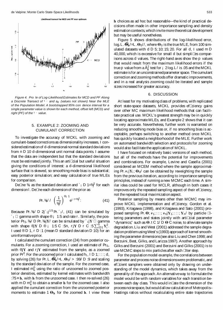dynamics describe these processes and often involve nonlinearpredatorndashprey interactions time lags arising from developmentand other factors that can produce complex dynamics (egMetz and Diekmann 1986 Tuljapurkar and Caswell 1997Gurney and Nisbet 1998)

Because of their relative dimensionalityof noises states ob-servations and replicates experimental population dynamicsproblemshave a different balance of ef ciency issues than otherstate-space or hidden-variables problems MC state-space re-search has typically considered methods for single long timeseries such as for nancial data (Carlin Polson and Stoffer1992 Shephard and Pitt 1997 Tanizaki and Mariano 1998Pitt and Shephard 1999 Durham and Gallant 2002) or sh-eries catch and survey records (Bjoslashrnstad Fromentin Stensethand Gjosaeter 1999 Meyer and Millar 1999 Millar and Meyer2000) At the other extreme MC methods for experimentaldatahave been applied to generalized linear mixed models wheredata are iid and the likelihood requires a MC integration overunknown random variables (Clayton 1996 McCulloch 1997Booth and Hobert 1999) Experimental population dynamicsdata mix these features in the form of short replicated time se-ries In addition realistic populationdynamics models are oftencontinuous in time or have a short time step so that the spaceof random disturbances entering the process may be of muchhigher dimension than the observationspace Also the aim hereis to calculate approximate likelihood ratio tests whereas mostMC state-space research has addressed nonexperimental set-tings with more focus on ltering and smoothing than on pa-rameter estimation and testing

I compare ve MC methods for likelihood maximizationTwo of the main approaches in the literature are MCEM (Weiand Tanner 1990 Chan and Ledolter 1995 McCulloch 1997Robert and Casella 1999 Booth and Hobert 1999) and MCLR(Geyer and Thompson 1992 Geyer 1994 1996 McCulloch1997) which both use alternating steps of MC sampling andlocal maximization (but see Levine and Casella 2001 for po-tential improvements) Two other natural candidates for theproblem are PF (Gordon et al 1993 Kitagawa 1996 Pitt andShephard 1999 Doucet et al 2001b) and basic MC integra-tion possibly with importance sampling which I call MC di-rect (MCD) The method developedhere MC kernel likelihood(MCKL) temporarily treats parameters as random variablesfor purposes of Markov Chain MC (MCMC) sampling andthen uses a weighted kernel density estimator to approximatea classical likelihood surface MCKL is related to kernel den-sity estimation of Bayesian posterior distributions (West 1993Chen 1994 Givens and Raftery 1996 Liu and West 2001) butthe approach here of using kernel density estimates to recoverthe classical likelihood surface for a state-space model appearsto be new

Next I introduce the MC likelihood methods in detailFor MCKL I discuss convergence MC error and smoothingmode bias zooming in by resampling near the mode to reducesmoothing bias and estimating smoothing bias from posteriorcumulants I then introduce an example population model andhypothetical experiment and compare maximum likelihoodconvergence of the different methods Finally I use a problemof multivariate standard deviation estimation to illustrate andevaluate the zooming and cumulant-basedcorrections

2 MONTE CARLO LIKELIHOOD METHODS

Suppose that there are n experimental units with data vec-tors Yi i D 1 n which include both multiple times andmultiple observation dimensions To be more explicit denoteYi D Yi1 YiT where Yit is a vector of observa-tions at time t and there is a xed set of observation timest D 1 T (For notational simplicity I assume the sameset of observation times for each replicate) The methods hererequire only that the model be amenable to various MC al-gorithms MCMC for the MCKL MCEM and MCLR meth-ods and sequential particle ltering for the PF method Foreach replicate i let ordm i be the unknown states or processnoises with probability density Prordm i and let PrYijordm i bethe probability density of observations given states Denoteordmi D ordm i1 ordm iT where ordm it are the process noisesfrom time t iexcl 1 to t which may include many model time steps(and noise values) between observation times

Each method aims to maximize the likelihood integral for thed-dimensional parameter vector 2

L2 DnY

iD1

ZPrYijordm iPrordm i dordm i (1)

or l2 D logL2 Although (1) makes sense with ordm as ei-ther states or process noises from here on I use it as processnoises and write Xordm for the states In other words PrYi jordm i

will usually involve a calculation of state dynamics from theprocess noises with the observation density related to the statevalues In the example that follows ordmrsquos are random environ-mental variations X is a time trajectory of dynamics for an agecohort model with a 1-day time step and Y is a time series ofestimates taken every 10 days of the abundance of several lifestages each of which is a summation of multiple age cohortsFor general introductionof each method I do not need to spec-ify dimensions for states noises or observations Treatment ofinitial conditions is assumed to be included in the notation Ifthese conditionsare xed then the state calculations start fromthem if they are random then they are included in the processnoises Dependence of probabilities on 2 is suppressed in thenotationFinally everything is written for continuousvariablesbut could be easily adapted to discrete variables

Only the MCD and PF methods estimate the likelihood with-out introducing an unknown constant For the other methodsafter estimating the maximum likelihood estimator (MLE) it isnecessary to estimate the likelihood at the MLE for purposesof likelihood ratio approximate hypothesis tests and I assumethat this is feasible For my populationdynamics example I dothis through an importance-sampled MC estimate of (1) withan estimate of each Prordm i jYi as the importance density foreach Prordm i (Shephard and Pitt 1997)

21 Monte Carlo Direct

The most obvious approach MCD draws a large sam-ple fordmj

i gmjD1 from each Prordm i and uses

l2 frac14nX

iD1

log

1m

mX

jD1

PriexclYi

shyshyordmj i

cent

(2)

This method suffers from the inef ciency of basic MC inte-gration a large variance of PrYi jordmj

i (Robert and Casella




j I can be




22 Particle Filter


PrYj2 DTY

t D1





PmjD1 PrYt jordmj

1 t j1 tiexcl1


PmjD1 PrYt jordmj






ordmj 1 t j1 t ordm







iD1

mX

jD1

1m

logPriexclYi ordm

j i

shyshy21cent

frac14nX

iD1





l2 iexcl l2S

DnX

iD1

log

microZPrYi ordm ij2


para (5)





iD1

log

mX

jD1

PrYi ordmj i j2

PrYi ordmj i j2S

(6)









Pr2

nY

iD1

PrYiordm i j2 (7)



CS

DZ

cent cent centZ

Pr2ordm1 ordmnj


where CS DR



OLh2 D 1m

mX

jD1

Khiexcl2 2j

centwj (9)

wj D1

Pr2j



QdlD1 Khl

2l acutel


1 h2d




g2L2 d2 DZ

g2L2

PrS2PrS2 d2 (10)


Zg2L2 d2 frac14

CS

m

mX

jD1

g2j

Pr2j (11)



31 Convergence









r OLh2 D 1m

mX

jD1

rKh2 iexcl 2j

Pr2j D 0 (12)






curren






currenlm

D1

CS


Pr2L2 d2

(15)








34 Smoothing Bias




0 D lLh2h

DZ sup3 Y

m6Dl

Ktm

acuteK 0tl


(16)


0 DZ sup3 Y

m 6Dl

Ktm

acuteK 0tl

hl

poundmicro

L2h iexclX

i

hi ti iL2h C 1

2

X

ij

hihj ti tj ij L2h

iexcl 1

6

X

ijk


paradt (17)


0 DdX

mD1

12hm lmL20

iexcldX

jD1

h2j

2

Aacute

ljjL20 CdX

mD1

12hm ljjmL20

C Oh4 (18)





S2




lm DC2


ASlm D


Ly2

PrSydy (19)


ASll D

1

h2l

QdmD1 hm

poundmicro

L2h2



i 6Dl

h2i ii

sup3L2h2

PrS2h

acute

C [K]diexcl1[K 02]h

2l ll

sup3L2h2

PrS2h

acuteC Oh4

para (20)

where [K] DR

Kt2 dt [K 0] DR


2] DR









micro1 C 1

6

X

ij k

middotij kHij ky 6

para (21)







1

2

X

ij



is approximately


f k

frac14 iexcl 12

X

ij

middotij k

poundiexcl6 C 62

hiexcl1centij

iexcl 6iexcl1ij

curren (24)


35 Choice of h




pdC11 C h2dC2





mhdC2h2 C 2d=2C1 (26)




QL2 D 1m Pr2

mX

jD1

Khiexcl22j

cent (27)




frac34 2Pr

1Cfrac34 2Pr

C h2 so that for

h2 gtfrac34 4

Pr1Cfrac342

Pr KhcurrenPrS










centnt (28)



cent (29)





(a)

(b)

(c)



AaC1a D

8gtgtgtlt

gtgtgt

SE a middot DE




(30)

and




A1a Draquo

macrSE t a D amax


(32)






(33)


and




Bsa D

8gtgtgtlt

gtgtgt



h0ssC1 a D DsC1 C 1

0 otherwise

(36)













LE





SnLE

E

(38)



[Qn


E[Qn

iD1 Prmacr 0ij2

0]SnLE

E qSEjS 0E

[Qn



E jSE

(39)



E D qS0E jSE




LE

E SLJ


LE

E SLJ






l2 frac14nX

iD1

log

micro1m

mX

jD1

PriexclYi

shyshyordm j i

cent Prordm j i

PrSi ordmj i

ordmj i raquo PrS

i ordm i (40)


m D 2000







43 Results





4 gt


(a)

(b)



MCEM 1K MCEM 5K)








Prfrac34l sup3

1

frac34 2l

acuteregiexcl1



PniD1 Y2








6 DISCUSSION












REFERENCES






























































































j I can be




22 Particle Filter


PrYj2 DTY

t D1





PmjD1 PrYt jordmj

1 t j1 tiexcl1


PmjD1 PrYt jordmj






ordmj 1 t j1 t ordm







iD1

mX

jD1

1m

logPriexclYi ordm

j i

shyshy21cent

frac14nX

iD1





l2 iexcl l2S

DnX

iD1

log

microZPrYi ordm ij2


para (5)





iD1

log

mX

jD1

PrYi ordmj i j2

PrYi ordmj i j2S

(6)









Pr2

nY

iD1

PrYiordm i j2 (7)



CS

DZ

cent cent centZ

Pr2ordm1 ordmnj


where CS DR



OLh2 D 1m

mX

jD1

Khiexcl2 2j

centwj (9)

wj D1

Pr2j



QdlD1 Khl

2l acutel


1 h2d




g2L2 d2 DZ

g2L2

PrS2PrS2 d2 (10)


Zg2L2 d2 frac14

CS

m

mX

jD1

g2j

Pr2j (11)



31 Convergence









r OLh2 D 1m

mX

jD1

rKh2 iexcl 2j

Pr2j D 0 (12)






curren






currenlm

D1

CS


Pr2L2 d2

(15)








34 Smoothing Bias




0 D lLh2h

DZ sup3 Y

m6Dl

Ktm

acuteK 0tl


(16)


0 DZ sup3 Y

m 6Dl

Ktm

acuteK 0tl

hl

poundmicro

L2h iexclX

i

hi ti iL2h C 1

2

X

ij

hihj ti tj ij L2h

iexcl 1

6

X

ijk


paradt (17)


0 DdX

mD1

12hm lmL20

iexcldX

jD1

h2j

2

Aacute

ljjL20 CdX

mD1

12hm ljjmL20

C Oh4 (18)





S2




lm DC2


ASlm D


Ly2

PrSydy (19)


ASll D

1

h2l

QdmD1 hm

poundmicro

L2h2



i 6Dl

h2i ii

sup3L2h2

PrS2h

acute

C [K]diexcl1[K 02]h

2l ll

sup3L2h2

PrS2h

acuteC Oh4

para (20)

where [K] DR

Kt2 dt [K 0] DR


2] DR









micro1 C 1

6

X

ij k

middotij kHij ky 6

para (21)







1

2

X

ij



is approximately


f k

frac14 iexcl 12

X

ij

middotij k

poundiexcl6 C 62

hiexcl1centij

iexcl 6iexcl1ij

curren (24)


35 Choice of h




pdC11 C h2dC2





mhdC2h2 C 2d=2C1 (26)




QL2 D 1m Pr2

mX

jD1

Khiexcl22j

cent (27)




frac34 2Pr

1Cfrac34 2Pr

C h2 so that for

h2 gtfrac34 4

Pr1Cfrac342

Pr KhcurrenPrS










centnt (28)



cent (29)





(a)

(b)

(c)



AaC1a D

8gtgtgtlt

gtgtgt

SE a middot DE




(30)

and




A1a Draquo

macrSE t a D amax


(32)






(33)


and




Bsa D

8gtgtgtlt

gtgtgt



h0ssC1 a D DsC1 C 1

0 otherwise

(36)













LE





SnLE

E

(38)



[Qn


E[Qn

iD1 Prmacr 0ij2

0]SnLE

E qSEjS 0E

[Qn



E jSE

(39)



E D qS0E jSE




LE

E SLJ


LE

E SLJ






l2 frac14nX

iD1

log

micro1m

mX

jD1

PriexclYi

shyshyordm j i

cent Prordm j i

PrSi ordmj i

ordmj i raquo PrS

i ordm i (40)


m D 2000







43 Results





4 gt


(a)

(b)



MCEM 1K MCEM 5K)








Prfrac34l sup3

1

frac34 2l

acuteregiexcl1



PniD1 Y2








6 DISCUSSION












REFERENCES
































































































Pr2

nY

iD1

PrYiordm i j2 (7)



CS

DZ

cent cent centZ

Pr2ordm1 ordmnj


where CS DR



OLh2 D 1m

mX

jD1

Khiexcl2 2j

centwj (9)

wj D1

Pr2j



QdlD1 Khl

2l acutel


1 h2d




g2L2 d2 DZ

g2L2

PrS2PrS2 d2 (10)


Zg2L2 d2 frac14

CS

m

mX

jD1

g2j

Pr2j (11)



31 Convergence









r OLh2 D 1m

mX

jD1

rKh2 iexcl 2j

Pr2j D 0 (12)






curren






currenlm

D1

CS


Pr2L2 d2

(15)








34 Smoothing Bias




0 D lLh2h

DZ sup3 Y

m6Dl

Ktm

acuteK 0tl


(16)


0 DZ sup3 Y

m 6Dl

Ktm

acuteK 0tl

hl

poundmicro

L2h iexclX

i

hi ti iL2h C 1

2

X

ij

hihj ti tj ij L2h

iexcl 1

6

X

ijk


paradt (17)


0 DdX

mD1

12hm lmL20

iexcldX

jD1

h2j

2

Aacute

ljjL20 CdX

mD1

12hm ljjmL20

C Oh4 (18)





S2




lm DC2


ASlm D


Ly2

PrSydy (19)


ASll D

1

h2l

QdmD1 hm

poundmicro

L2h2



i 6Dl

h2i ii

sup3L2h2

PrS2h

acute

C [K]diexcl1[K 02]h

2l ll

sup3L2h2

PrS2h

acuteC Oh4

para (20)

where [K] DR

Kt2 dt [K 0] DR


2] DR









micro1 C 1

6

X

ij k

middotij kHij ky 6

para (21)







1

2

X

ij



is approximately


f k

frac14 iexcl 12

X

ij

middotij k

poundiexcl6 C 62

hiexcl1centij

iexcl 6iexcl1ij

curren (24)


35 Choice of h




pdC11 C h2dC2





mhdC2h2 C 2d=2C1 (26)




QL2 D 1m Pr2

mX

jD1

Khiexcl22j

cent (27)




frac34 2Pr

1Cfrac34 2Pr

C h2 so that for

h2 gtfrac34 4

Pr1Cfrac342

Pr KhcurrenPrS










centnt (28)



cent (29)





(a)

(b)

(c)



AaC1a D

8gtgtgtlt

gtgtgt

SE a middot DE




(30)

and




A1a Draquo

macrSE t a D amax


(32)






(33)


and




Bsa D

8gtgtgtlt

gtgtgt



h0ssC1 a D DsC1 C 1

0 otherwise

(36)













LE





SnLE

E

(38)



[Qn


E[Qn

iD1 Prmacr 0ij2

0]SnLE

E qSEjS 0E

[Qn



E jSE

(39)



E D qS0E jSE




LE

E SLJ


LE

E SLJ






l2 frac14nX

iD1

log

micro1m

mX

jD1

PriexclYi

shyshyordm j i

cent Prordm j i

PrSi ordmj i

ordmj i raquo PrS

i ordm i (40)


m D 2000







43 Results





4 gt


(a)

(b)



MCEM 1K MCEM 5K)








Prfrac34l sup3

1

frac34 2l

acuteregiexcl1



PniD1 Y2








6 DISCUSSION












REFERENCES
































































































curren






currenlm

D1

CS


Pr2L2 d2

(15)








34 Smoothing Bias




0 D lLh2h

DZ sup3 Y

m6Dl

Ktm

acuteK 0tl


(16)


0 DZ sup3 Y

m 6Dl

Ktm

acuteK 0tl

hl

poundmicro

L2h iexclX

i

hi ti iL2h C 1

2

X

ij

hihj ti tj ij L2h

iexcl 1

6

X

ijk


paradt (17)


0 DdX

mD1

12hm lmL20

iexcldX

jD1

h2j

2

Aacute

ljjL20 CdX

mD1

12hm ljjmL20

C Oh4 (18)





S2




lm DC2


ASlm D


Ly2

PrSydy (19)


ASll D

1

h2l

QdmD1 hm

poundmicro

L2h2



i 6Dl

h2i ii

sup3L2h2

PrS2h

acute

C [K]diexcl1[K 02]h

2l ll

sup3L2h2

PrS2h

acuteC Oh4

para (20)

where [K] DR

Kt2 dt [K 0] DR


2] DR









micro1 C 1

6

X

ij k

middotij kHij ky 6

para (21)







1

2

X

ij



is approximately


f k

frac14 iexcl 12

X

ij

middotij k

poundiexcl6 C 62

hiexcl1centij

iexcl 6iexcl1ij

curren (24)


35 Choice of h




pdC11 C h2dC2





mhdC2h2 C 2d=2C1 (26)




QL2 D 1m Pr2

mX

jD1

Khiexcl22j

cent (27)




frac34 2Pr

1Cfrac34 2Pr

C h2 so that for

h2 gtfrac34 4

Pr1Cfrac342

Pr KhcurrenPrS










centnt (28)



cent (29)





(a)

(b)

(c)



AaC1a D

8gtgtgtlt

gtgtgt

SE a middot DE




(30)

and




A1a Draquo

macrSE t a D amax


(32)






(33)


and




Bsa D

8gtgtgtlt

gtgtgt



h0ssC1 a D DsC1 C 1

0 otherwise

(36)













LE





SnLE

E

(38)



[Qn


E[Qn

iD1 Prmacr 0ij2

0]SnLE

E qSEjS 0E

[Qn



E jSE

(39)



E D qS0E jSE




LE

E SLJ


LE

E SLJ






l2 frac14nX

iD1

log

micro1m

mX

jD1

PriexclYi

shyshyordm j i

cent Prordm j i

PrSi ordmj i

ordmj i raquo PrS

i ordm i (40)


m D 2000







43 Results





4 gt


(a)

(b)



MCEM 1K MCEM 5K)








Prfrac34l sup3

1

frac34 2l

acuteregiexcl1



PniD1 Y2








6 DISCUSSION












REFERENCES


































































































micro1 C 1

6

X

ij k

middotij kHij ky 6

para (21)







1

2

X

ij



is approximately


f k

frac14 iexcl 12

X

ij

middotij k

poundiexcl6 C 62

hiexcl1centij

iexcl 6iexcl1ij

curren (24)


35 Choice of h




pdC11 C h2dC2





mhdC2h2 C 2d=2C1 (26)




QL2 D 1m Pr2

mX

jD1

Khiexcl22j

cent (27)




frac34 2Pr

1Cfrac34 2Pr

C h2 so that for

h2 gtfrac34 4

Pr1Cfrac342

Pr KhcurrenPrS










centnt (28)



cent (29)





(a)

(b)

(c)



AaC1a D

8gtgtgtlt

gtgtgt

SE a middot DE




(30)

and




A1a Draquo

macrSE t a D amax


(32)






(33)


and




Bsa D

8gtgtgtlt

gtgtgt



h0ssC1 a D DsC1 C 1

0 otherwise

(36)













LE





SnLE

E

(38)



[Qn


E[Qn

iD1 Prmacr 0ij2

0]SnLE

E qSEjS 0E

[Qn



E jSE

(39)



E D qS0E jSE




LE

E SLJ


LE

E SLJ






l2 frac14nX

iD1

log

micro1m

mX

jD1

PriexclYi

shyshyordm j i

cent Prordm j i

PrSi ordmj i

ordmj i raquo PrS

i ordm i (40)


m D 2000







43 Results





4 gt


(a)

(b)



MCEM 1K MCEM 5K)








Prfrac34l sup3

1

frac34 2l

acuteregiexcl1



PniD1 Y2








6 DISCUSSION












REFERENCES

































































































centnt (28)



cent (29)





(a)

(b)

(c)



AaC1a D

8gtgtgtlt

gtgtgt

SE a middot DE




(30)

and




A1a Draquo

macrSE t a D amax


(32)






(33)


and




Bsa D

8gtgtgtlt

gtgtgt



h0ssC1 a D DsC1 C 1

0 otherwise

(36)













LE





SnLE

E

(38)



[Qn


E[Qn

iD1 Prmacr 0ij2

0]SnLE

E qSEjS 0E

[Qn



E jSE

(39)



E D qS0E jSE




LE

E SLJ


LE

E SLJ






l2 frac14nX

iD1

log

micro1m

mX

jD1

PriexclYi

shyshyordm j i

cent Prordm j i

PrSi ordmj i

ordmj i raquo PrS

i ordm i (40)


m D 2000







43 Results





4 gt


(a)

(b)



MCEM 1K MCEM 5K)








Prfrac34l sup3

1

frac34 2l

acuteregiexcl1



PniD1 Y2








6 DISCUSSION












REFERENCES





























































































A1a Draquo

macrSE t a D amax


(32)






(33)


and




Bsa D

8gtgtgtlt

gtgtgt



h0ssC1 a D DsC1 C 1

0 otherwise

(36)













LE





SnLE

E

(38)



[Qn


E[Qn

iD1 Prmacr 0ij2

0]SnLE

E qSEjS 0E

[Qn



E jSE

(39)



E D qS0E jSE




LE

E SLJ


LE

E SLJ






l2 frac14nX

iD1

log

micro1m

mX

jD1

PriexclYi

shyshyordm j i

cent Prordm j i

PrSi ordmj i

ordmj i raquo PrS

i ordm i (40)


m D 2000







43 Results





4 gt


(a)

(b)



MCEM 1K MCEM 5K)








Prfrac34l sup3

1

frac34 2l

acuteregiexcl1



PniD1 Y2








6 DISCUSSION












REFERENCES






























































































SnLE

E

(38)



[Qn


E[Qn

iD1 Prmacr 0ij2

0]SnLE

E qSEjS 0E

[Qn



E jSE

(39)



E D qS0E jSE




LE

E SLJ


LE

E SLJ






l2 frac14nX

iD1

log

micro1m

mX

jD1

PriexclYi

shyshyordm j i

cent Prordm j i

PrSi ordmj i

ordmj i raquo PrS

i ordm i (40)


m D 2000







43 Results





4 gt


(a)

(b)



MCEM 1K MCEM 5K)








Prfrac34l sup3

1

frac34 2l

acuteregiexcl1



PniD1 Y2








6 DISCUSSION












REFERENCES































































































43 Results





4 gt


(a)

(b)



MCEM 1K MCEM 5K)








Prfrac34l sup3

1

frac34 2l

acuteregiexcl1



PniD1 Y2








6 DISCUSSION












REFERENCES

































































































Prfrac34l sup3

1

frac34 2l

acuteregiexcl1



PniD1 Y2








6 DISCUSSION












REFERENCES


































































































REFERENCES



























































































monte carlo state-space likelihoods by weighted posterior...

Documents