monte carlo simulations of elastic scattering with .... comput. phys. doi:...

Commun. Comput. Phys.doi: 10.4208/cicp.210211.270511a

Vol. 11, No. 5, pp. 1618-1642May 2012

Monte Carlo Simulations of Elastic Scattering

with Applications to DC and High Power Pulsed

Magnetron Sputtering for Ti3SiC2

Jurgen Geiser1,∗ and Sven Blankenburg2

1 Department of Mathematics, Humboldt-Universitat zu Berlin, D-10099 Berlin,Germany.2 Department of Physics, Humboldt-Universitat zu Berlin, D-10099 Berlin,Germany.

Received 21 February 2011; Accepted (in revised version) 27 May 2011

Communicated by Haiqing Lin

Available online 9 January 2012

Abstract. We simulate the particle transport in a thin film deposition process madeby PVD (physical vapor deposition) and present several models for projectile and tar-get collisions in order to compute the mean free path and the differential cross section(angular distribution of scattered projectiles) of the scattering process. A detailed de-scription of collision models is of the highest importance in Monte Carlo simulationsof high power impulse magnetron sputtering and DC sputtering. We derive an equa-tion for the mean free path for arbitrary interactions (cross sections) that includes therelative velocity between the particles. We apply our results to two major interactionmodels: hard sphere interaction & screened Coulomb interaction. Both types of inter-action separate DC sputtering from HIPIMS.

AMS subject classifications: 80M31, 60J20, 65N74, 65C05, 65C35, 65C40

Key words: DC sputtering, MAX-phases, mean free path, particle in cell Monte Carlo collisions,Monte Carlo Markov chain.

1 Introduction

The main reason for studying the collision processes of elastic scattering is the need for areliable physical description of the interactions between ions and a plasma (backgroundgas) in high power pulsed magnetron sputtering processes for the creation of uniform,stoichiometric thin films. MAX-phases experienced a renaissance in the mid 1990s, when

∗Corresponding author. Email addresses: [email protected] (J. Geiser), [email protected] (S. Blankenburg)

http://www.global-sci.com/ 1618 c©2012 Global-Science Press

J. Geiser and S. Blankenburg / Commun. Comput. Phys., 11 (2012), pp. 1618-1642 1619

Barsoum synthesized relatively phase-pure samples of the MAX-phase Ti3SiC2, and dis-covered a material with a unique combination of metallic and ceramic properties: it ex-hibited high electrical and thermal conductivity, and it was extremely resistant to oxida-tion and thermal shock, and so is very attractive for industrial applications like protonexchange fuel cells (PEFC). These stoichiometries (MAX-phases) are described by thegeneral formula Mn+1AXn, where M is an early transition metal (Sc, Ti, V, Cr, Zr, Nb,Mo, Hf, Ta), A is an A-group element (Al, Si, P, S, Ga, Ge, As, Cd, In, Sn, Ti, Pb), andX is either Carbon and/or Nitrogen. The different MAX stoichiometries are often re-ferred to as 211 (n= 1), 312 (n= 2). Recent developments have led to a new method ofsynthesizing thin films of MAX-phases on a substrate (workpiece): high power impulsemagnetron sputtering (HIPIMS or HPPMS), see [1–4]. The most important ingredientin sputtering processes is a plasma, i.e., a partially ionized gas, which, at macroscopicscales, is electrically neutral. If a material body such as a substrate is immersed in aplasma it will acquire a potential slightly negative with respect to ground. This effectis known as a floating potential. The physical reason for this is the higher mobility ofelectrons than that of ions. Hence, more electrons reach the substrate surface than ions.A very sensitive quantity in sputtering processes (with respect to the experimental setup:gas-pressure, temperature, target-material, etc.) is the sputtering yield, which describesthe ratio of atoms ejected from a target surface per incident ion. The sputtering yieldcan take almost any value from 0.1 up to 10. To optimize production, one is generallyinterested in obtaining values for the sputtering yield as high as possible. In order toobtain a well defined film stoichiometry at the substrate, one has to take into accountthe transport mechanism of the sputtered particles within the plasma. This can be doneeither within a macroscopic description of the transport phenomena, i.e., the solution ofthe advection–diffusion equation, or at a microscopic scale, via Monte Carlo simulationsof the transport phenomena. This paper deals almost exclusively with the last approach,in the future, the ultimate goal of our work will be to link both approaches to each other(this will be presented in future papers).

This paper is organized as follows: In Section 2 we describe the concept of mean freepath and derive, on the basis of the kinetic theory, an appropriate expression for the meanfree path of an external particle (projectile) that is probing an ensemble of target particlesthat constitute an ideal gas (background gas). The main modification to standard meanfree paths is to allow of initially moving targets. Section 3 studies, from first principles,the concept of differential cross sections. In Section 4 we present our Monte Carlo methodbased on a pathway model, see [5], and perform several simulations of direct current(DC) and high power pulsed magnetron sputtering (HIPIMS). At the end, in Section 5,we summarize our results and discuss perspectives for future work.

2 Collision model: mean free path

The mean free path or average distance between collisions for a gas molecule may beestimated from kinetic theory. If one assumes the gas consists of hard spheres (non over-

1620 J. Geiser and S. Blankenburg / Commun. Comput. Phys., 11 (2012), pp. 1618-1642

lapping spheres), then the effective collision area is given by

σ=π(d1+d2)2=πD2. (2.1)

In time δt, the area sweeps out a volume of Vinteraction and the number of collisions can beestimated from the number of target molecules (nV) that are in that volume

Vinteraction=σvδt. (2.2)

The expression for the mean free path,

λ=|vproj|δt

VinteractionnV=

|vproj|δt

πD2vδtnV=

1

πD2nV, (2.3)

is a good approximation, but it suffers from a significant flaw—it assumes the targetobject’s being at rest, which is of course nonsense, physically. We introducing the relativevelocity between the gas objects

vrel =√

2v. (2.4)

Here the√

2 results from the molecular speed distribution of a mono atomic ideal gas(Maxwell–Boltzmann distribution). We therefore have the expression

λ=1√

2πD2nV

. (2.5)

The number of molecules per unit volume can be determined from the state equation ofthe gas

pV=(1+B1+B2+···)RT. (2.6)

If one assumes an ideal gas (non interacting and non overlapping gas particles) one canneglect the so called higher virial coefficients (B1+B2+···). Inserting the state equationfor an ideal gas into (2.5), one gets

λ=(1)RT√

2πD2NA p. (2.7)

Here R is the gas constant and NA is Avogadro’s number. This is an approximation forthe mean free path of an atom/molecule of an ideal gas. In our problem, however, wehave to calculate the mean free path of an external particle (projectile) which is not amember of the background gas (ideal gas). This can be done by modifying the averagerelative velocity between projectile and target. This is done in the next part.


2.1 The mean relative velocity between projectiles and targets

The background gas is assumed to be Maxwell distributed in velocity (this is motivatedby the assumption of an ideal gas). Because the background particles are an ensemble(with statistically distributed velocities) one can just speak of a mean relative velocity< |vrel |>=< |vproj−vtarget|>, which can be calculated via:

< |vrel |>=∫ ∫ ∫

V|vproj−vtarget|Z

(vtarget

)dvtarget, (2.8)

where Z is the three-dimensional Maxwell distribution given by

Z(vtarget

)=(A/π)3/2 1

2√

2exp

(−Avtarget

2), (2.9)

with the abbreviation A = Mtarget/2kBT. A complete derivation of the solution can befound in the Appendix. The result is

|vrel |=

[(s+ 1

2s

)erf(s)+ 1√

πexp

(−s2

)]

3s×|vproj|, (2.10)

with s= a√

A (scalar) and a= |vproj|. We now want to discuss a few special cases.If the velocity of the projectile is very small, |vproj| ≈ 0, then s ≈ 0 and therefore the

following approximation holdsvrel ≈vtarget. (2.11)

If the target objects are identical to the projectile objects (same mass and same meanvelocity), then the following limit holds

|vrel |≈1.41|vtarget |, (2.12)

which gives the factor√

2≈1.41 and leads to the mean free path of an element of a monoatomic ideal gas (as expected). However, the general expression for the mean free pathof a projectile probing into an ideal gas with pressure Pgas and temperature T is given by

λproj =3

4π

s[(s+ 1

2s

)erf(s)+ 1√

πexp(−s2)

] kBT(

Rion+Rtarget

)2Pgas

. (2.13)

There are a few things to say about this expression. First, the main assumption that thebackground gas (ensemble of target particles) is an ideal gas, is valid only within the highvacuum regime, i.e., small target density. Second, the interaction between the projectileand target atoms are assumed to be of hard sphere type, i.e., purely geometrical. If theprojectile is a free particle between the interactions, its Hamilton function is

H=p2

2Mproj=E. (2.14)


In this case one can easily compute a= |vproj|=√

2E/Mproj.. There follows immediately

s= a√

A=

√E

kBT

√Mtarget

Mproj. (2.15)

In appropriate units (atomic units) the scalar s is

s=107.7242

√E[eV]

T[K]

√Mtarget

Mproj. (2.16)

Therefore the mean free path in units of cm is given by:

λproj[cm]=s[(

s+ 12s

)erf(s)+ 1√

πexp(−s2)

] · 3.297cm·T[K](

Rion[pm]+Rtarget[pm])2

Pgas[mbar]. (2.17)

In [2], a formula for the mean free path of ions surrounded by an ideal gas of pressurepar is used and given by

λ[cm]=4.39cm·T[K]√(

1+ MionMtarget

)(rion[pm]+rtarget [pm]

)2ptarget[mbar]

. (2.18)

Table 1 shows the mean free path for ions at E = 3 eV and T = 300K and gas pressurep=4×10−3 mbar.

Table 1: mean free paths for the different sputter species.

Ion Eq. (2.17) Eq. (2.18)carbon (12) 12.96 cm 15.18 cmsilicon (28) 7.52 cm 7.71 cm

titanium (48) 5.03 cm 4.55 cm

In a sputtering process, the ions obey a kinetic energy distribution as well as anangular-distribution at the target. Because of different transport mechanisms, an ionloses to some extent its initial kinetic energy. The ions of a sputter process can there-fore be classified into three groups. First, the ballistic group, such that any member of theballistic group travels from the target to the substrate in a straight line because no colli-sions occur. The transition group is characterized by the observation that the path of theion is not a straight line and therefore the ions of this group undergo some collisions butstill retain some of their initial energy. The last group is the thermalized or diffusive group,where any member of this group has completely lost its initial kinetic energy. The motionof such an ion is therefore described by a random walk. The typical distances betweenthe target and the substrate are of the order of 5–15 cm. Hence, at low argon pressures


10−3

10−2

10−1

100

101

0

2

4

6

8

10

12

14mean free path particle @ argon(rigid sphere)

ion energy [eV]

mea

n fr

ee p

ath

[cm

]

C

Si

Ti

temperature: T=300 KAr pressure: p=0.004 mbar

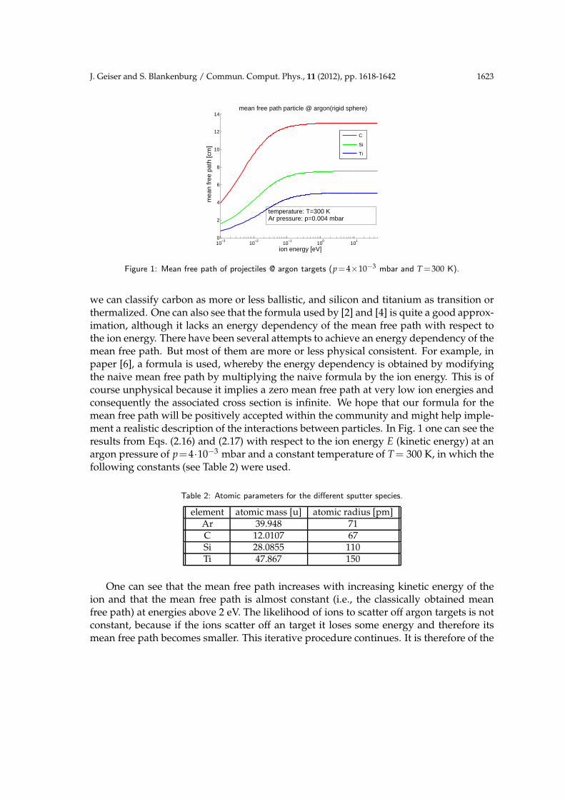
Figure 1: Mean free path of projectiles @ argon targets (p=4×10−3 mbar and T=300 K).

we can classify carbon as more or less ballistic, and silicon and titanium as transition orthermalized. One can also see that the formula used by [2] and [4] is quite a good approx-imation, although it lacks an energy dependency of the mean free path with respect tothe ion energy. There have been several attempts to achieve an energy dependency of themean free path. But most of them are more or less physical consistent. For example, inpaper [6], a formula is used, whereby the energy dependency is obtained by modifyingthe naive mean free path by multiplying the naive formula by the ion energy. This is ofcourse unphysical because it implies a zero mean free path at very low ion energies andconsequently the associated cross section is infinite. We hope that our formula for themean free path will be positively accepted within the community and might help imple-ment a realistic description of the interactions between particles. In Fig. 1 one can see theresults from Eqs. (2.16) and (2.17) with respect to the ion energy E (kinetic energy) at anargon pressure of p=4·10−3 mbar and a constant temperature of T= 300 K, in which thefollowing constants (see Table 2) were used.

Table 2: Atomic parameters for the different sputter species.

element atomic mass [u] atomic radius [pm]Ar 39.948 71C 12.0107 67Si 28.0855 110Ti 47.867 150

One can see that the mean free path increases with increasing kinetic energy of theion and that the mean free path is almost constant (i.e., the classically obtained meanfree path) at energies above 2 eV. The likelihood of ions to scatter off argon targets is notconstant, because if the ions scatter off an target it loses some energy and therefore itsmean free path becomes smaller. This iterative procedure continues. It is therefore of the


highest importance in situations in which one has to deal with multiple scattering, as isthe case if the sputter-target and the substrate.

3 Collision model: Differential cross section & angular

distribution

With the help of the mean free path λ one is able, within a Monte Carlo approach, todetermine the collision frequency. But several questions are unanswered by a knowledgeof the mean free path. If one is interested in a detailed description (kinematic) of thescattering process, one has to work out the differential cross section. We propose twodescriptions; both are, within their limits, applicable. In the first model, we assume thetarget particle is initially at rest, whereas the second model will loosen this restriction.

3.1 Scattering with initially fixed targets

If the projectile velocity is much higher than the target velocity one can assume the tar-get atoms are initially at rest. Describing the scattering process with the center of masssystem (CMS) simplifies the calculations. The theoretical analysis of such a scatteringprocess can be found in almost any text book on classical mechanics such as [7]. We usespherical coordinates, wherein θ,φ describes the coordinates in the laboratory and Θ, Φ

are the coordinates in the CMS. The ratio

ρ=Mproj

Mtarget

vt,1

vrel,1(3.1)

can be used to connect the scattering angles in the laboratory and the CMS (radial sym-metric scattering potential)

cosθ=cosΘ+ρ√

1+2ρcosΘ+ρ2. (3.2)

The transformation from CMS coordinates to laboratory coordinates brings in the Jaco-bian as an extra factor:

σ(θ)=σ(Θ)sinΘ

sinθ

∣∣∣∣d(Θ,Φ)

d(θ,φ)

∣∣∣∣. (3.3)

Because Φ=φ the Jacobian reduces to

σ(θ)=σ(Θ)

∣∣∣∣dcosΘ

dcosθ

∣∣∣∣. (3.4)

With the help of Eq. (3.2) one gets

σ(θ)=σ(Θ)

(1+2ρcosΘ+ρ2

)3/2

1+ρcosΘ. (3.5)


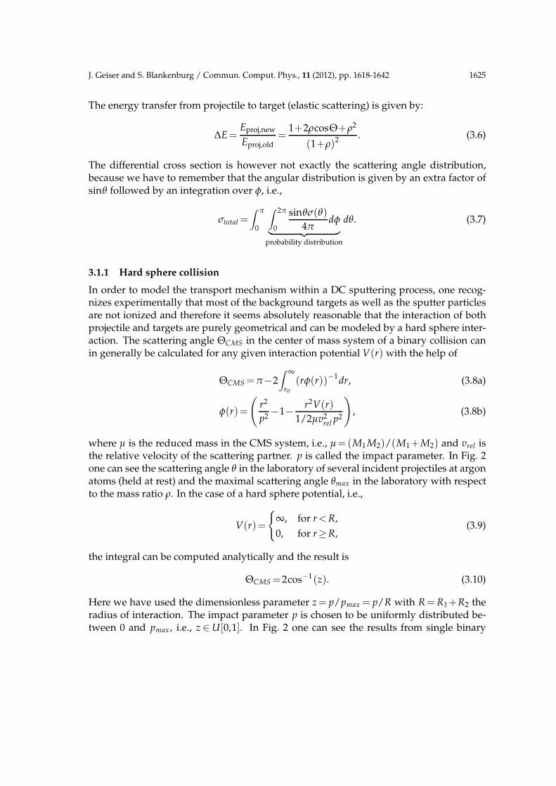
The energy transfer from projectile to target (elastic scattering) is given by:

∆E=Eproj,new

Eproj,old=

1+2ρcosΘ+ρ2

(1+ρ)2. (3.6)

The differential cross section is however not exactly the scattering angle distribution,because we have to remember that the angular distribution is given by an extra factor ofsinθ followed by an integration over φ, i.e.,

σtotal =∫ π

0

∫ 2π

0

sinθσ(θ)

4πdφ

︸︷︷︸probability distribution

dθ. (3.7)

3.1.1 Hard sphere collision

In order to model the transport mechanism within a DC sputtering process, one recog-nizes experimentally that most of the background targets as well as the sputter particlesare not ionized and therefore it seems absolutely reasonable that the interaction of bothprojectile and targets are purely geometrical and can be modeled by a hard sphere inter-action. The scattering angle ΘCMS in the center of mass system of a binary collision canin generally be calculated for any given interaction potential V(r) with the help of

ΘCMS =π−2∫ ∞

r0

(rφ(r))−1dr, (3.8a)

φ(r)=

(r2

p2−1− r2V(r)

1/2µv2rel p2

), (3.8b)

where µ is the reduced mass in the CMS system, i.e., µ=(M1M2)/(M1+M2) and vrel isthe relative velocity of the scattering partner. p is called the impact parameter. In Fig. 2one can see the scattering angle θ in the laboratory of several incident projectiles at argonatoms (held at rest) and the maximal scattering angle θmax in the laboratory with respectto the mass ratio ρ. In the case of a hard sphere potential, i.e.,

V(r)=

{∞, for r<R,

0, for r≥R,(3.9)

the integral can be computed analytically and the result is

ΘCMS =2cos−1(z). (3.10)

Here we have used the dimensionless parameter z= p/pmax = p/R with R=R1+R2 theradius of interaction. The impact parameter p is chosen to be uniformly distributed be-tween 0 and pmax, i.e., z ∈ U[0,1]. In Fig. 2 one can see the results from single binary


0 20 40 60 80 100 120 140 160 1800

100

200

300

400

500

600

700

800

900

1000

scattering angle ΘCMS

[degree]

rela

tive

prob

abili

ty d

istr

ibut

ion

total MC−events:100000

0 20 40 60 80 100 120 140 160 1800

2000

4000

6000

8000

10000

12000

14000

16000

18000

scattering angle ΘLAB

[degree]

rela

tive

prob

abili

ty d

istr

ibut

ion


C12

at Ar39

Si28

at Ar39

Ti48

at Ar39

0 0.2 0.4 0.6 0.8 1 1.2 1.4 1.6 1.8 220

40

60

80

100

120

140

160

180

mass ratio ρ

θ max

[deg

ree]

numerical estimation of θmax

0 0.1 0.2 0.3 0.4 0.5 0.6 0.7 0.8 0.9 10

1000

2000

3000

4000

5000

6000

7000

8000

9000

transfered energy amount

rela

tive

prob

abili

ty d

istr

ibut

ion


C12

at Ar39

Si28

at Ar39

Ti48

at Ar39

0 0.1 0.2 0.3 0.4 0.5 0.6 0.7 0.8 0.9 10

20

40

60

80

100

120

140

160

180Hard Sphere Scattering

parameter z=b/bmax

scat

terin

g an

gle

ΘC

MS [d

egre

e]

Upper left: scattering angle distribution of ΘCMSin the CMS system and upper right: Monte Carloresults of the scattering angle probability distribu-tion in the laboratory system. Middle left: numer-ical determination of the maximal scattering angleθmax in the laboratory and Middle right: prob-ability distribution of the transferred energy viaMonte Carlo simulations. Lower left: scatteringangle ΘCMS with respect to the scattering parame-ter z.

Figure 2: Results from one hard sphere collision (targets initially at rest).

collisions for the sputter species C, Si, and Ti within the framework of hard sphere colli-sions. One can see that as long as the projectile mass is smaller than the target mass allscattering angles are allowed. However, this changes if the mass ratio becomes greaterthan 1. In this case only a cone of scattering directions is allowed, and the opening angleof the cone decreases with increasing mass ratio. In the case of titanium projectiles at ar-gon targets, only scattering angles between 0 and θmax≈60 degrees are allowed. Titaniumprojectiles are therefore subjected to forward scattering and the cone angle is around 120degrees. The above approach is quite satisfactory if one assumes highly energetic pro-jectiles (with respect to target velocity) and the suppression of multi-scattering events. A


proper description of the kinematics should include the random motion of the target pro-jectiles and therefore an energy dependency for the differential cross section. The totalcross section has to be unchanged, because the total area per target cannot depend on therelative velocity of the target and projectile, because the total cross section is an intrinsicquantity.

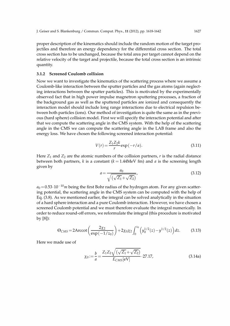
3.1.2 Screened Coulomb collision

Now we want to investigate the kinematics of the scattering process where we assume aCoulomb-like interaction between the sputter particles and the gas atoms (again neglect-ing interactions between the sputter particles). This is motivated by the experimentallyobserved fact that in high power impulse magnetron sputtering processes, a fraction ofthe background gas as well as the sputtered particles are ionized and consequently theinteraction model should include long range interactions due to electrical repulsion be-tween both particles (ions). Our method of investigation is quite the same as in the previ-ous (hard sphere) collision model. First we will specify the interaction potential and afterthat we compute the scattering angle in the CMS system. With the help of the scatteringangle in the CMS we can compute the scattering angle in the LAB frame and also theenergy loss. We have chosen the following screened interaction potential:

V(r)=Z1Z2k

rexp(−r/a). (3.11)

Here Z1 and Z2 are the atomic numbers of the collision partners, r is the radial distancebetween both partners, k is a constant (k = 1.44MeV fm) and a is the screening lengthgiven by

a=a0√(√

Z1+√

Z2

) , (3.12)

a0=0.53·10−10m being the first Bohr radius of the hydrogen atom. For any given scatter-ing potential, the scattering angle in the CMS system can be computed with the help ofEq. (3.8). As we mentioned earlier, the integral can be solved analytically in the situationof a hard sphere interaction and a pure Coulomb interaction. However, we have chosen ascreened Coulomb potential and we must therefore evaluate the integral numerically. Inorder to reduce round-off errors, we reformulate the integral (this procedure is motivatedby [8]):

ΘCMS =2Arccot

(2χ2

exp(−1/z0)

)+2χ0χ2

∫ z0

0

(y1/2

0 (z)−y1/2(z))

dz. (3.13)

Here we made use of

χ0 :=b

a=

Z1Z2

√(√Z1+

√Z2

)

ECMS[eV]·27.17, (3.14a)


χ2 :=p

b=

p[10−10m]ECMS[eV]

Z1Z2· 1

14.4, (3.14b)

ECMS =

((1+1/2s)erf(s)+1/

√πexp

(−s2

))2

(1+

Mproj

Mtarget

)9s2

·Eproj, (3.14c)

y0(z)=1−(χ0χ2)2z2−χ0zexp(−1/z0), (3.14d)

y(z)=1−(χ0χ2)2 z2−χ0zexp(−1/z), z= r/a. (3.14e)

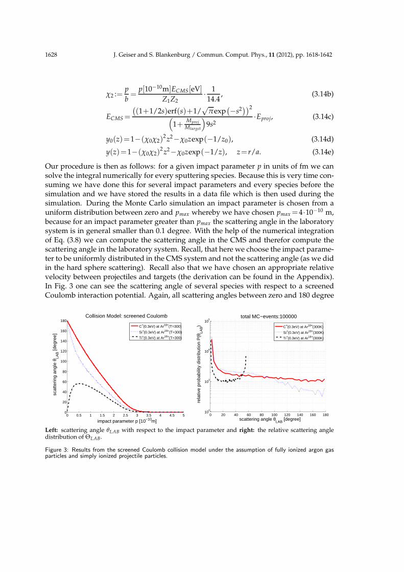
Our procedure is then as follows: for a given impact parameter p in units of fm we cansolve the integral numerically for every sputtering species. Because this is very time con-suming we have done this for several impact parameters and every species before thesimulation and we have stored the results in a data file which is then used during thesimulation. During the Monte Carlo simulation an impact parameter is chosen from auniform distribution between zero and pmax whereby we have chosen pmax =4·10−10 m,because for an impact parameter greater than pmax the scattering angle in the laboratorysystem is in general smaller than 0.1 degree. With the help of the numerical integrationof Eq. (3.8) we can compute the scattering angle in the CMS and therefor compute thescattering angle in the laboratory system. Recall, that here we choose the impact parame-ter to be uniformly distributed in the CMS system and not the scattering angle (as we didin the hard sphere scattering). Recall also that we have chosen an appropriate relativevelocity between projectiles and targets (the derivation can be found in the Appendix).In Fig. 3 one can see the scattering angle of several species with respect to a screenedCoulomb interaction potential. Again, all scattering angles between zero and 180 degree

0 0.5 1 1.5 2 2.5 3 3.5 4 4.5 50

20

40

60

80

100

120

140

160

180

impact parameter p [10−10m]

scat

terin

g an

gle

θ LAB [d

egre

e]

Collision Model: screened Coulomb

C+(0.3eV) at Ar18+(T=300)

Si+(0.3eV) at Ar18+(T=300)

Ti+(0.3eV) at Ar18+(T=300)

0 20 40 60 80 100 120 140 160 18010

2

103

104

105

scattering angle θLAB

[degree]

rela

tive

prob

abili

ty d

istr

ibut

ion

P(θ

LAB)


C+(0.3eV) at Ar18+(300K)

Si+(0.3eV) at Ar18+(300K)

Ti+(0.3eV) at Ar18+(300K)

Left: scattering angle θLAB with respect to the impact parameter and right: the relative scattering angledistribution of ΘLAB.

Figure 3: Results from the screened Coulomb collision model under the assumption of fully ionized argon gasparticles and simply ionized projectile particles.


are possible for projectiles with a mass smaller than the target mass. For projectiles with amass greater than the target mass there exists a maximum scattering angle and thereforethe scattering occurs only with an scattering cone of finite opening angle, i.e., forwardscattering in the laboratory system will be preferred for titanium. In Fig. 3 one can seethe functional dependency of the scattering angle in the laboratory stem with respectto the impact parameter as well as the relative probability distribution of the scatteringangle θLAB in the laboratory system.

4 Monte Carlo simulations

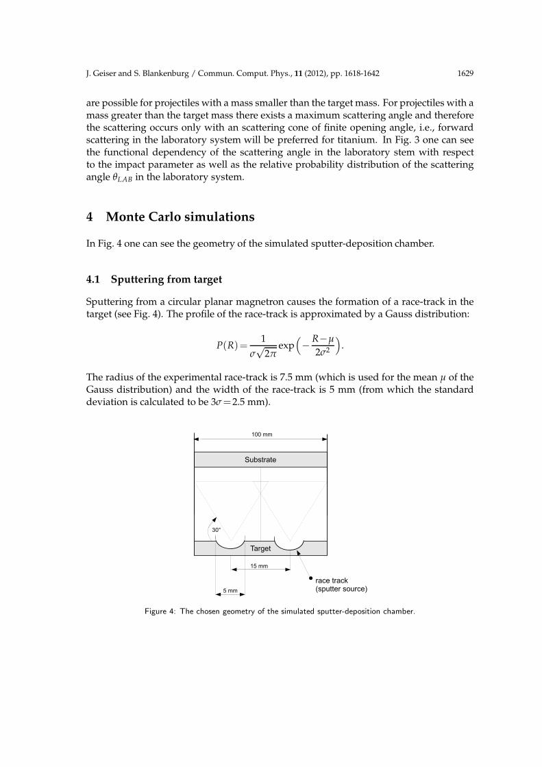
In Fig. 4 one can see the geometry of the simulated sputter-deposition chamber.

4.1 Sputtering from target

Sputtering from a circular planar magnetron causes the formation of a race-track in thetarget (see Fig. 4). The profile of the race-track is approximated by a Gauss distribution:

P(R)=1

σ√

2πexp

(− R−µ

2σ2

).

The radius of the experimental race-track is 7.5 mm (which is used for the mean µ of theGauss distribution) and the width of the race-track is 5 mm (from which the standarddeviation is calculated to be 3σ=2.5 mm).

Figure 4: The chosen geometry of the simulated sputter-deposition chamber.


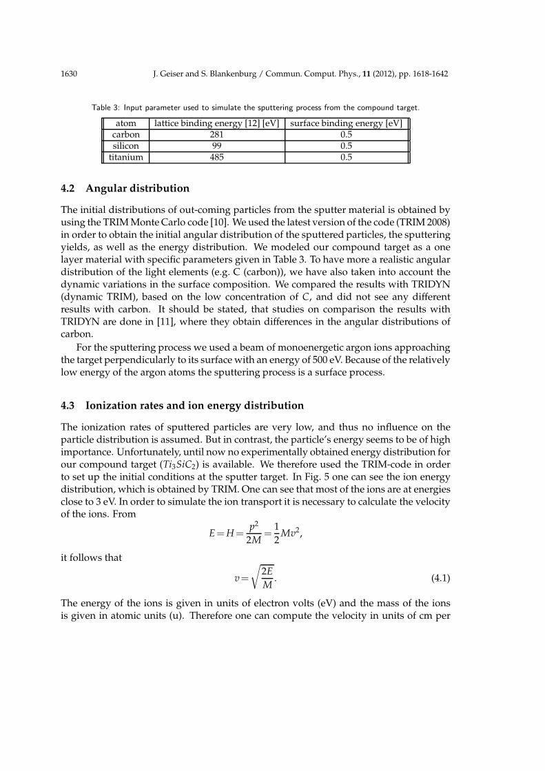
Table 3: Input parameter used to simulate the sputtering process from the compound target.

atom lattice binding energy [12] [eV] surface binding energy [eV]carbon 281 0.5silicon 99 0.5

titanium 485 0.5

4.2 Angular distribution

The initial distributions of out-coming particles from the sputter material is obtained byusing the TRIM Monte Carlo code [10]. We used the latest version of the code (TRIM 2008)in order to obtain the initial angular distribution of the sputtered particles, the sputteringyields, as well as the energy distribution. We modeled our compound target as a onelayer material with specific parameters given in Table 3. To have more a realistic angulardistribution of the light elements (e.g. C (carbon)), we have also taken into account thedynamic variations in the surface composition. We compared the results with TRIDYN(dynamic TRIM), based on the low concentration of C, and did not see any differentresults with carbon. It should be stated, that studies on comparison the results withTRIDYN are done in [11], where they obtain differences in the angular distributions ofcarbon.

For the sputtering process we used a beam of monoenergetic argon ions approachingthe target perpendicularly to its surface with an energy of 500 eV. Because of the relativelylow energy of the argon atoms the sputtering process is a surface process.

4.3 Ionization rates and ion energy distribution

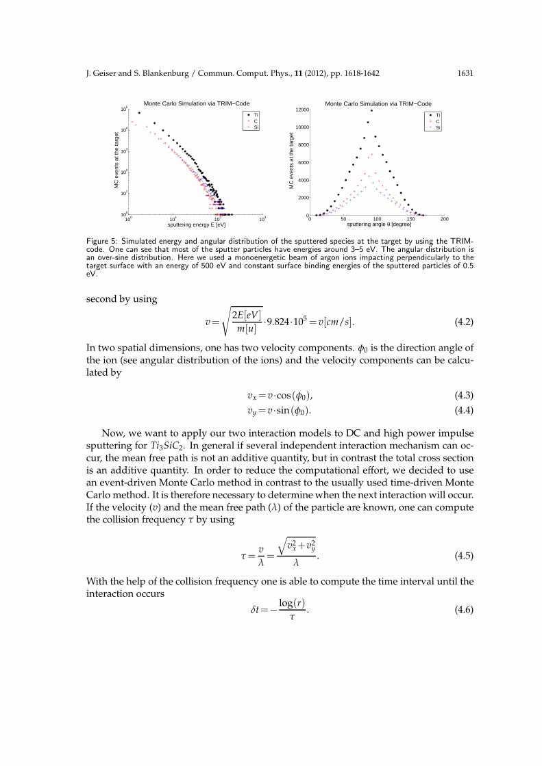
The ionization rates of sputtered particles are very low, and thus no influence on theparticle distribution is assumed. But in contrast, the particle’s energy seems to be of highimportance. Unfortunately, until now no experimentally obtained energy distribution forour compound target (Ti3SiC2) is available. We therefore used the TRIM-code in orderto set up the initial conditions at the sputter target. In Fig. 5 one can see the ion energydistribution, which is obtained by TRIM. One can see that most of the ions are at energiesclose to 3 eV. In order to simulate the ion transport it is necessary to calculate the velocityof the ions. From

E=H=p2

2M=

1

2Mv2,

it follows that

v=

√2E

M. (4.1)

The energy of the ions is given in units of electron volts (eV) and the mass of the ionsis given in atomic units (u). Therefore one can compute the velocity in units of cm per


100

101

102

103

100

101

102

103

104

105

Monte Carlo Simulation via TRIM−Code

MC

eve

nts

at th

e ta

rget

sputtering energy E [eV]

TiCSi

0 50 100 150 2000

2000

4000

6000

8000

10000

12000Monte Carlo Simulation via TRIM−Code

MC

eve

nts

at th

e ta

rget

sputtering angle θ [degree]

TiCSi

Figure 5: Simulated energy and angular distribution of the sputtered species at the target by using the TRIM-code. One can see that most of the sputter particles have energies around 3–5 eV. The angular distribution isan over-sine distribution. Here we used a monoenergetic beam of argon ions impacting perpendicularly to thetarget surface with an energy of 500 eV and constant surface binding energies of the sputtered particles of 0.5eV.

second by using

v=

√2E[eV]

m[u]·9.824·105 =v[cm/s]. (4.2)

In two spatial dimensions, one has two velocity components. φ0 is the direction angle ofthe ion (see angular distribution of the ions) and the velocity components can be calcu-lated by

vx =v·cos(φ0), (4.3)

vy=v·sin(φ0). (4.4)

Now, we want to apply our two interaction models to DC and high power impulsesputtering for Ti3SiC2. In general if several independent interaction mechanism can oc-cur, the mean free path is not an additive quantity, but in contrast the total cross sectionis an additive quantity. In order to reduce the computational effort, we decided to usean event-driven Monte Carlo method in contrast to the usually used time-driven MonteCarlo method. It is therefore necessary to determine when the next interaction will occur.If the velocity (v) and the mean free path (λ) of the particle are known, one can computethe collision frequency τ by using

τ=v

λ=

√v2

x+v2y

λ. (4.5)

With the help of the collision frequency one is able to compute the time interval until theinteraction occurs

δt=− log(r)

τ. (4.6)


Mworkpiece M+workpiece

Mtotal

M+Target

SMG

ηt 1−η t

Workpiece

Target

Lost

+TargetG

SMM +

+

+

+

+

+

ζζ

1−β

βσ

1−σ

M+Target

1−η t


Mtotal

SMG

+G

ζζ

1−β

Target

SMM

β

1−σ

ηtLost

++

+

+

+

+

Mtotal

SMG

G 1G 2σ

Workpiece

Target

Species 1

+

+

+

+

++

Lostηt

Target

SMM

β

1−σ

ζζ

1−β

+G


M+Target

1−η t

Species 2

λ

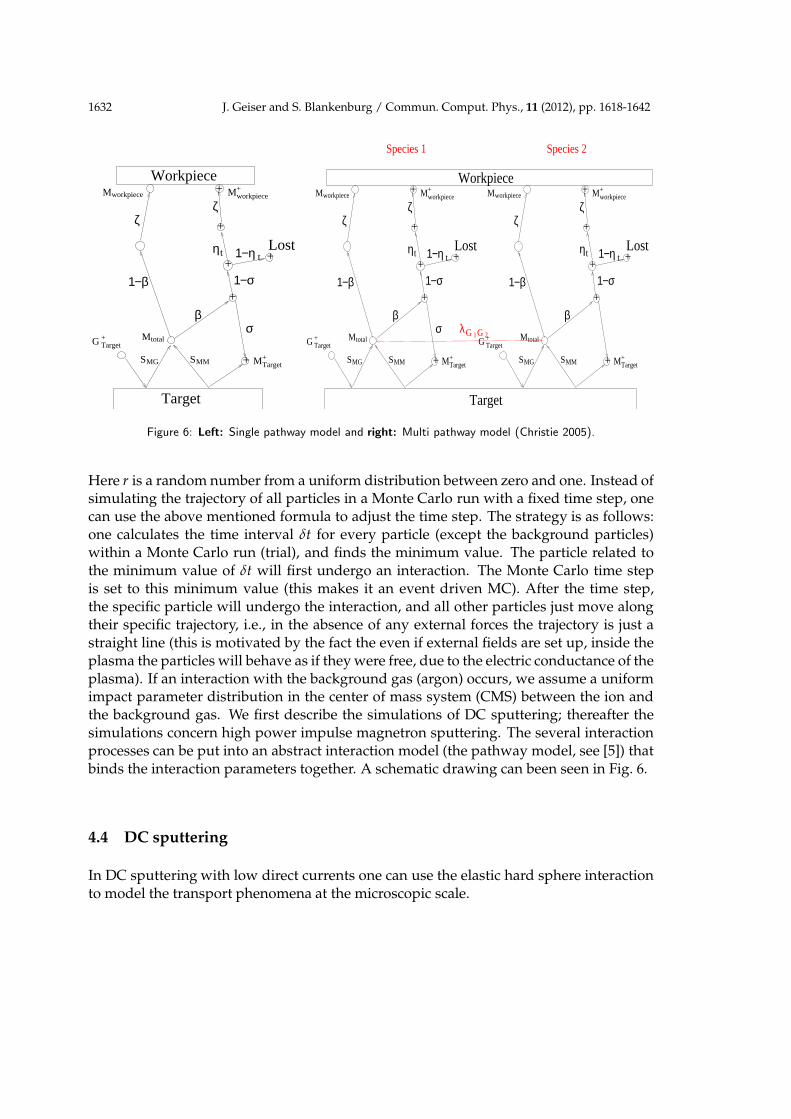
Figure 6: Left: Single pathway model and right: Multi pathway model (Christie 2005).

Here r is a random number from a uniform distribution between zero and one. Instead ofsimulating the trajectory of all particles in a Monte Carlo run with a fixed time step, onecan use the above mentioned formula to adjust the time step. The strategy is as follows:one calculates the time interval δt for every particle (except the background particles)within a Monte Carlo run (trial), and finds the minimum value. The particle related tothe minimum value of δt will first undergo an interaction. The Monte Carlo time stepis set to this minimum value (this makes it an event driven MC). After the time step,the specific particle will undergo the interaction, and all other particles just move alongtheir specific trajectory, i.e., in the absence of any external forces the trajectory is just astraight line (this is motivated by the fact the even if external fields are set up, inside theplasma the particles will behave as if they were free, due to the electric conductance of theplasma). If an interaction with the background gas (argon) occurs, we assume a uniformimpact parameter distribution in the center of mass system (CMS) between the ion andthe background gas. We first describe the simulations of DC sputtering; thereafter thesimulations concern high power impulse magnetron sputtering. The several interactionprocesses can be put into an abstract interaction model (the pathway model, see [5]) thatbinds the interaction parameters together. A schematic drawing can been seen in Fig. 6.

4.4 DC sputtering

In DC sputtering with low direct currents one can use the elastic hard sphere interactionto model the transport phenomena at the microscopic scale.


Table 4: Experimental setup parameter concerning the first experiment.

Parameter ValueTemperature (T) 300 K

Ar-pressure (pAr) 4·10−3 mbarS-T-distance (d) variable from 1 cm to 24 cm

Table 5: Experimental setup concerning the second experiment.

Parameter ValueTemperature (T) 300 K

Ar-pressure (pAr) 4·10−3 mbarS–T distance (d) variable from 1 cm to 24 cm

4.4.1 First experiment: Only hard sphere interaction

In Fig. 7 the results of 100,000 Monte Carlo events are shown, in which we used theexperimental setup parameters in Table 4.

4.5 High power impulse magnetron sputtering

In HIPIMS one can assume that at least a fraction of particles (sputter particles as wellas target particles) are ionized. Unfortunately, there is no specific relation between pulseduration and/or pulse height and the percentage of ionized particles. The next results aretherefore very academic. In our first experiment concerning HIPIMS we assume that allgas particles and sputter particles are simply ionized. This is of course a realistic propertyfor the gas particles (argon) but not for the sputter particles.

4.5.1 Second experiment: Only Coulomb interaction

If one assumes all sputter particles and all gas particles are at least simply ionized, thenthe interaction is completely described by the Coulomb or screened Coulomb interac-tion. For sake of simplicity, we assume only simply ionized particles. The results fromMonte Carlo simulations can be seen in Fig. 8 whereby we used the experimental setupparameters in Table 5.

4.5.2 Third experiment: Mixed interactions

If one assumes the sputter particles consist of ionized as well as neutral atoms two inter-actions with the background gas can occur: hard sphere collisions if one of the collisionparticles is neutral, and Coulomb interactions if both collision particles are at least simplyionized. We assume the particles are only simply ionized and therefore we have chosenthe following (see Table 6) effective atomic numbers Ze f f with respect to the Slater rulesin atomic physics.


−10 −5 0 5 1010

0

101

102

103

104

distance from target axis [cm]

MC

−ev

ents

at w

orkp

iece

(1cmDC)total MC−events:87002

CSiTi

−10 −5 0 5 100

10

20

30

40

50

60

70

80

90

100


atom

−%


CSiTi

S−T−distance:1 cmAr pressure:0.004 mbar

−10 −5 0 5 1010

0

101

102

103

104


MC

−ev

ents

at w

orkp

iece


CSiTi

−10 −5 0 5 100

10

20

30

40

50

60

70

80


atom

−%


CSiTi


−10 −5 0 5 1010

1

102

103

104


MC

−ev

ents

at w

orkp

iece


CSiTi

−10 −5 0 5 100

10

20

30

40

50

60

70


atom

−%


C

Si

Ti


−10 −5 0 5 1010

1

102

103


MC

−ev

ents

at w

orkp

iece


CSiTi

−10 −5 0 5 1010

20

30

40

50

60

70


atom

−%


C

Si

Ti


Left: registered Monte Carlo events at the workpiece and right: stoichiometric composition at the workpiecefor several target–substrate distances in cm in which we assumed a pure hard sphere interaction betweenthe sputter particles and the gas particles.

Figure 7: Results from the first experiment.


−10 −5 0 5 1010

0

101

102

103

104


MC

−ev

ents

at w

orkp

iece

(1cmsc)total MC−events:87002

CSiTi

−10 −5 0 5 100

10

20

30

40

50

60

70

80

90

100


atom

−%


CSiTi


−10 −5 0 5 1010

0

101

102

103

104


MC

−ev

ents

at w

orkp

iece


CSiTi

−10 −5 0 5 100

10

20

30

40

50

60

70

80


atom

−%


CSiTiS−T−distance:4 cm

Ar pressure:0.004 mbar

−10 −5 0 5 1010

0

101

102

103

104


MC

−ev

ents

at w

orkp

iece


CSiTi

−10 −5 0 5 1010

20

30

40

50

60

70


atom

−%


C

Si

Ti


−10 −5 0 5 1010

1

102

103

104


MC

−ev

ents

at w

orkp

iece


CSiTi

−10 −5 0 5 1010

20

30

40

50

60

70


atom

−%


C

Si

Ti


Left: Registered Monte Carlo events at the workpiece and right: stoichiometric film composition at theworkpiece for several target–substrate distances in cm in which we assumed a pure Coulomb interactionbetween the sputter particles and the gas particles (simple ionized species). One can easily see the effectof the two sputter sources on the stoichiometric film composition at small substrate–target distances. Thiseffect smears out at far distances.

Figure 8: Results from the second experiment.


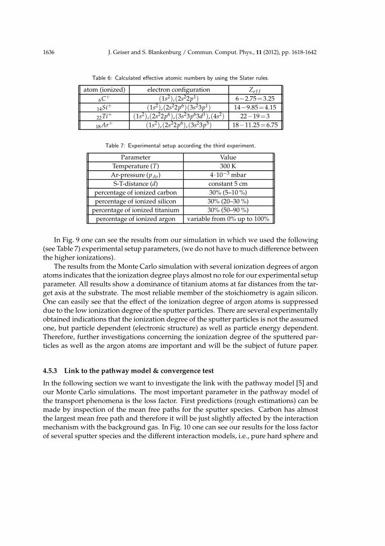
Table 6: Calculated effective atomic numbers by using the Slater rules.

atom (ionized) electron configuration Ze f f

6C+ (1s2),(2s22p1) 6−2.75=3.25

14Si+ (1s2),(2s22p6)(3s23p1) 14−9.85=4.15

22Ti+ (1s2),(2s22p6),(3s23p63d1),(4s2) 22−19=3

18 Ar+ (1s2),(2s22p6),(3s23p5) 18−11.25=6.75

Table 7: Experimental setup according the third experiment.

Parameter Value

Temperature (T) 300 K

Ar-pressure (pAr) 4·10−3 mbar

S-T-distance (d) constant 5 cm

percentage of ionized carbon 30% (5–10 %)

percentage of ionized silicon 30% (20–30 %)

percentage of ionized titanium 30% (50–90 %)

percentage of ionized argon variable from 0% up to 100%

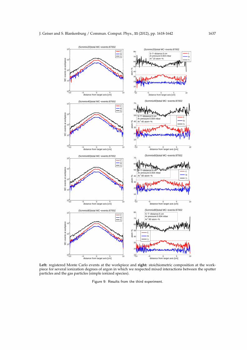
In Fig. 9 one can see the results from our simulation in which we used the following(see Table 7) experimental setup parameters, (we do not have to much difference betweenthe higher ionizations).

The results from the Monte Carlo simulation with several ionization degrees of argonatoms indicates that the ionization degree plays almost no role for our experimental setupparameter. All results show a dominance of titanium atoms at far distances from the tar-get axis at the substrate. The most reliable member of the stoichiometry is again silicon.One can easily see that the effect of the ionization degree of argon atoms is suppresseddue to the low ionization degree of the sputter particles. There are several experimentallyobtained indications that the ionization degree of the sputter particles is not the assumedone, but particle dependent (electronic structure) as well as particle energy dependent.Therefore, further investigations concerning the ionization degree of the sputtered par-ticles as well as the argon atoms are important and will be the subject of future paper.

4.5.3 Link to the pathway model & convergence test

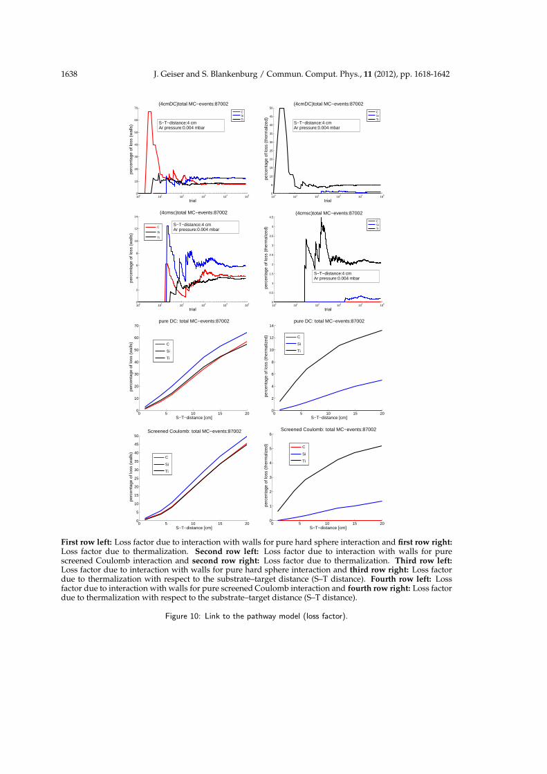
In the following section we want to investigate the link with the pathway model [5] andour Monte Carlo simulations. The most important parameter in the pathway model ofthe transport phenomena is the loss factor. First predictions (rough estimations) can bemade by inspection of the mean free paths for the sputter species. Carbon has almostthe largest mean free path and therefore it will be just slightly affected by the interactionmechanism with the background gas. In Fig. 10 one can see our results for the loss factorof several sputter species and the different interaction models, i.e., pure hard sphere and


−10 −5 0 5 1010

0

101

102

103

104


MC

−ev

ents

at w

orkp

iece

(5cmmix20)total MC−events:87002

CSiTi

−10 −5 0 5 100

10

20

30

40

50

60

70

80


atom

−%


C

Si

Ti

S−T−distance:5 cmAr pressure:0.004 mbarAr+:20 atom−%

−10 −5 0 5 1010

0

101

102

103

104


MC

−ev

ents

at w

orkp

iece


CSiTi

−10 −5 0 5 100

10

20

30

40

50

60

70


atom

−%


C

Si

Ti


−10 −5 0 5 1010

0

101

102

103

104


MC

−ev

ents

at w

orkp

iece


CSiTi

−10 −5 0 5 100

10

20

30

40

50

60

70


atom

−%


C

Si

Ti


−10 −5 0 5 1010

0

101

102

103

104


MC

−ev

ents

at w

orkp

iece


CSiTi

−10 −5 0 5 1010

20

30

40

50

60

70

80


atom

−%


C

Si

Ti


Left: registered Monte Carlo events at the workpiece and right: stoichiometric composition at the work-piece for several ionization degrees of argon in which we respected mixed interactions between the sputterparticles and the gas particles (simple ionized species).

Figure 9: Results from the third experiment.


100

101

102

103

104

105

0

10

20

30

40

50

60

70

trial

perc

enta

ge o

f los

s (w

alls

)


CSiTi


100

101

102

103

104

105

0

5

10

15

20

25

30

35

40

45

50

trial

perc

enta

ge o

f los

s (t

herm

aliz

ed)


CSiTi


100

101

102

103

104

105

0

2

4

6

8

10

12

14

trial

perc

enta

ge o

f los

s (w

alls

)


C

Si

Ti


100

101

102

103

104

105

0

0.5

1

1.5

2

2.5

3

3.5

4

4.5

trial

perc

enta

ge o

f los

s (t

herm

aliz

ed)


CSiTi


0 5 10 15 200

10

20

30

40

50

60

70

S−T−distance [cm]

perc

enta

ge o

f los

s (w

alls

)

pure DC: total MC−events:87002

C

Si

Ti

0 5 10 15 200

2

4

6

8

10

12

14


perc

enta

ge o

f los

s (t

herm

aliz

ed)

pure DC: total MC−events:87002

C

Si

Ti

0 5 10 15 200

5

10

15

20

25

30

35

40

45

50


perc

enta

ge o

f los

s (w

alls

)

Screened Coulomb: total MC−events:87002

C

Si

Ti

0 5 10 15 200

1

2

3

4

5

6


perc

enta

ge o

f los

s (t

herm

aliz

ed)

Screened Coulomb: total MC−events:87002

C

Si

Ti

First row left: Loss factor due to interaction with walls for pure hard sphere interaction and first row right:Loss factor due to thermalization. Second row left: Loss factor due to interaction with walls for purescreened Coulomb interaction and second row right: Loss factor due to thermalization. Third row left:Loss factor due to interaction with walls for pure hard sphere interaction and third row right: Loss factordue to thermalization with respect to the substrate–target distance (S–T distance). Fourth row left: Lossfactor due to interaction with walls for pure screened Coulomb interaction and fourth row right: Loss factordue to thermalization with respect to the substrate–target distance (S–T distance).

Figure 10: Link to the pathway model (loss factor).


pure screened Coulomb (described by the first two experiments). One can easily see thatthe values for the loss factor are almost constant after some equilibrium trials. This indi-cates a way of observing the convergence behavior of our Monte Carlo algorithm. Thus,with the help of the loss factor we can estimate the minimum Monte Carlo trials withina simulation and conclude from the equilibrium tendency that our implementation wasdone correctly. It is important to remember that the equilibrium MC time (number of MCtrials) for the loss factor differs from Monte Carlo run to Monte Carlo run even with thesame experimental setup parameter. We see that 50,000 Monte Carlo trials (events) arealmost enough to equilibrate the system, i.e., reach convergence. One can also see thesensitivity of the loss factor with respect to different interaction mechanism between tar-get atoms and projectiles. The loss factor for Coulomb interactions in general is smallerthan the loss factor for hard sphere interactions.

5 Conclusion

So far, we have developed an appropriate Monte Carlo method based on a pathwaymodel for interactions between sputtered particles and a background gas, assumed tobe an ideal gas. We have set up a novel equation for the mean free path which incorpo-rates all physical parameter such as temperature and gas pressure, but most importantlyit respects the movement of the target atoms, i.e., the argon particles. With the help ofour theoretical investigations we performed several Monte Carlo simulations for directcurrent (DC) and high power impulse magnetron sputtering (HIPIMS). The results fromour simulations are qualitatively in agreement with experimentally obtained film com-positions at the substrate as in the target composition. We were thus able to show thatin DC sputtering the main interaction between the sputter particles and the backgroundgas is of hard sphere type, i.e., purely geometrical. In HIPIMS a mixture of hard sphereand Coulomb interaction takes place. Unfortunately, the lack of experimentally obtaineddata concerning the ionization degree of the sputtered particles and the background gasforbids a direct comparison between simulation and experiments. In the future we hopeto extract the ionization degree from first principles or by data fitting to experimentallyobtained results. The effect of moving targets on the differential cross section, i.e., theangular distribution of sputtered particles, cannot be neglected. The effect of initiallymoving targets (with respect to the Maxwell velocity distribution) is especially impor-tant within the thermal group, i.e., with an energy ratio of the target and projectile ofabout one. Carbon and silicon are almost not members of the thermal group (because oftheir large mean free path). But titanium is a member of the thermal or diffusive group.In the case of a pure hard sphere interaction between argon and titanium, almost all scat-tering angles in the laboratory system can occur (in contrast to the initially resting targetapproach). The calculation and implementation of the initially moving target approachis in progress and includes an appropriate Monte Carlo Markov chain method.


Acknowledgments

This work was funded by the Federal Ministry of Education and Research under contractnumber 03 SF 0325 A. We additionally thank Dipl.-Ing. Martin Balzer, FEM, SchwabischGmund, Germany for his discussions and for inspiring this work.

Appendix: Derivation of the mean relative velocity

Within the framework of statistical mechanics, the mean value of an observable O can becomputed via

<O>=

∫ ∫O(q,p)Z(q,p;H)d3Nqd3N p∫ ∫

pZ(q,p;H)d3Nqd3N p. (A.1)

With q the canonical coordinates and p the canonical momenta of an N-particle system,i.e., with Hamiltonian H(q,p) and obeying Hamiltonian’s equations of motion. The prob-ability distribution Z depends on the total Hamiltonian H of the system. Within thecanonical ensemble one has the following relation

Z=exp

(−H(q,p)

kBT

). (A.2)

With p = mv and the assumption of an ideal gas, the Hamilton function for the back-ground gas is constructed by means of the kinetic energies of the gas particles

H=N

∑i=1

p2i

2mi. (A.3)

If O=O(p) then the coordinate integration gives a volume factor in the numerator anddenominator and therefore no contribution. The momentum integration can be doneimmediately and results in Gaussian integrals. The result for the mean relative velocityis therefore given by

<O=vrel >=∫ ∫ ∫

V|vproj−vtarget|Z

(vtarget

)dvtarget, (A.4)

with Z=(A/π)3/2 12√

2exp(−Av2) the reduced partition function (Maxwell distribution)

and A=Mtarget/2kBT. By substituting u=vtarget−vproj and du=vtarget one gets

< |vrel |>=∫ ∫ ∫

V|u|exp

(−Av2

proj−2Avproju−Au2)

du

=(A/π)3/2exp

(−Avproj

2)

2√

2︸︷︷︸=:C(a,A)

∫ ∫ ∫

V|u|exp

(−2Avproju−Au2

)du. (A.5)


By using spherical coordinates with r = |u|, a= |vproj.| and vproj ·u= |vproj|·|u|cosθ onegets

< |vrel |>=C(a,A)∫ ∞

0

∫ 2π

0

∫ π

0rexp

(−Ar2−2A·a·r·cosθ

)r2sinθdθdφdr

=2πC(a,A)∫ ∞

0r3∫ π

0exp

(−Ar2−2Aarcosθ

)sinθdθdr. (A.6)

The double integral on the right hand side can be evaluated and its solution is

∫ ∞

0r3∫ π

0exp

(−Ar2−2Aarcosθ

)sinθdθdr

=

(Aπ

)3/2exp

(−a2 A

)

2√

2

2√

Aa+(2Aa2+1

)exp

(a2 A

)√πerf

(a√

A)

4aA5/2

. (A.7)

After some simplification the mean relative velocity is

< |vrel |>=

(2a+ 1

Aa

)erf(

a√

A)+

2exp(−a2A)√A√

π

4√

2. (A.8)

Here we made use of the scalar s := a√

A.With a= |vproj| the final result for the mean relative velocity between projectiles prob-

ing into a mono-atomic ideal gas is given by

< |vrel |>=

[(s+ 1

2s

)erf(s)+ 1√

πexp

(−s2

)]

3s×|vproj|. (A.9)

References

[1] J. Alami, P. Eklund, J. Emmerlich, O. Wilhelmsson, U. Jansson, H. Hogberg, L. Hultman,and U. Helmersson, High-power impulse magnetron sputtering of Ti-Si-C thin films from aTi3SiC2 compound target, Thin Solid Films 515 (2006), 1731-1736.

[2] P. Eklund, M. Beckers, U. Jansson, H. Hogberg, and L. Hultman, The Mn+1AXn phases:Materials science and thin-film processing, Thin Solid Films 518 (2010), 1851-1878.

[3] P. Eklund, M. Beckers, J. Frodelius, H. Hogberg, and L. Hultman, Magnetron sputtering ofTi3SiC2 thin films from a compound target, J. Vac. Sci. Technol. A 25 (2007), 1381–1388.

[4] K. Sarakinos, J. Alami, and S. Konstantinidis, High power pulsed magnetron sputtering: Areview on scientific and engineering state of the art, Surf. Coat. Tech. 204 (2010), 1661-1684.

[5] D.J. Christie, Target material pathways model for high power pulsed magnetron sputtering,J. Vac. Sci. Technol. 23 (2005), 330–335.

[6] S. Mahiheu, G. Buyle, D. Depla, S. Heirwegh, P. Ghekiere, and R. De Gryse, Monte Carlosimulation of the transport of atoms in DC magnetron sputtering, Nucl. Instrum. MethodsPhys. Res. B 243 (2006), 313–319.


[7] H. Goldstein, Classical Mechanics, 2nd edition, Addison-Wesley: Reading, MA, USA, 1980.[8] E. Everhart, G. Stone, and R.J. Carbone, Classical calculation of differential cross section

for scattering from a Coulomb potential with exponential screening, Phys. Rev. 99 (1955),1287–1290.

[9] A. Russek, Effect of target gas temperature on the scattering cross section, Phys. Rev. 120(1960), 1536–1542.

[10] J.P. Biersack and W. Eckstein, Sputtering studies with the Monte Carlo Program TRIM.SP,Appl. Phys. A 34 (1984), 73–94.

[11] J. Neidhardt, S. Mraz, J.M. Schneider, E. Strub, W. Bohne, J. Rohrich, and C. Mitterer, Exper-iment and simulation of the compositional evolution of TiB thin films deposited by sputter-ing of a compound target, J. Appl. Phys. 104 (2008), 063304.

[12] D.P. Riley, D.J. O’Connor, P. Dastoor, N. Brack, and P.J. Pigram, Comparative analysis ofTi3SiC2 and associated compounds using x-ray diffraction and x-ray photoelectron spec-troscopy, J. Phys. D: Appl. Phys. 35 (2002), 1603-1611.

monte carlo simulations of elastic scattering with .... comput. phys. doi:...

Documents