monte carlo search in games
TRANSCRIPT
Project Number: CS-GXS-0901
Monte Carlo Search in Games
a Major Qualifying Project Reportsubmitted to the Faculty of the
WORCESTER POLYTECHNIC INSTITUTE
in partial fulfillment of the requirements for theDegree of Bachelor of Science by
David A. Anderson
April 29, 2009
Professor Gabor N. Sarkozy, Major Advisor
Professor Stanley M. Selkow, Co-Advisor

Abstract
In this project we implemented four training algorithms designed to improve random
playouts in Monte Carlo simulations. We applied these algorithms to the game Go using a
small board (9x9), and 3x3 patterns to parameterize our playout policy. We analyzed the
effectiveness of these algorithms against a purely random policy, both with and without deep
Monte Carlo searches.
i

Acknowledgements
This project would not have been possible without the generous help of the following people:
• Professor Gabor N. Sarkozy, main advisor
• Professor Stanley M. Selkow, co-advisor
• Levente Kocsis, SZTAKI MLHCI liaison
In addition, special thanks to:
• MTA SZTAKI
• Worcester Polytechnic Institute
• Lukasz Lew for the libEGO project
• Sensei’s Library for a wealth of Go knowledge
• Isaac Edwards for countless Go discussions
ii

Contents
Appendices ii
1 Background 1
1.1 Motivation . . . . . . . . . . . . . . . . . . . . . . . . . . . . . . . . . . . . . 1
1.2 Rules and History of Go . . . . . . . . . . . . . . . . . . . . . . . . . . . . . 2
1.3 Computer Go . . . . . . . . . . . . . . . . . . . . . . . . . . . . . . . . . . . 7
1.4 Monte-Carlo Search . . . . . . . . . . . . . . . . . . . . . . . . . . . . . . . . 8
2 Algorithms 12
2.1 Introduction . . . . . . . . . . . . . . . . . . . . . . . . . . . . . . . . . . . . 12
2.2 Softmax Policy . . . . . . . . . . . . . . . . . . . . . . . . . . . . . . . . . . 14
2.3 Apprenticeship Learning . . . . . . . . . . . . . . . . . . . . . . . . . . . . . 15
2.4 Policy Gradient Reinforcement Learning . . . . . . . . . . . . . . . . . . . . 17
2.5 Policy Gradient Simulation Balancing . . . . . . . . . . . . . . . . . . . . . . 18
2.6 Two Step Simulation Balancing . . . . . . . . . . . . . . . . . . . . . . . . . 19
2.7 Development . . . . . . . . . . . . . . . . . . . . . . . . . . . . . . . . . . . 20
3 Experiments 23
3.1 Setup . . . . . . . . . . . . . . . . . . . . . . . . . . . . . . . . . . . . . . . . 23
3.2 libEGO Uniform Random . . . . . . . . . . . . . . . . . . . . . . . . . . . . 26
3.3 Apprenticeship Learning . . . . . . . . . . . . . . . . . . . . . . . . . . . . . 27
iii
3.4 Policy Gradient Reinforcement Learning . . . . . . . . . . . . . . . . . . . . 30
3.5 Policy Gradient Simulation Balancing . . . . . . . . . . . . . . . . . . . . . . 32
3.6 Two Step Simulation Balancing . . . . . . . . . . . . . . . . . . . . . . . . . 34
4 Conclusions 37
A Development Notes 40
iv
Figures, Tables, and Algorithms
List of Figures
1.1 Liberties . . . . . . . . . . . . . . . . . . . . . . . . . . . . . . . . . . . . . . 3
1.2 Capturing . . . . . . . . . . . . . . . . . . . . . . . . . . . . . . . . . . . . . 4
1.3 Life and death. . . . . . . . . . . . . . . . . . . . . . . . . . . . . . . . . . . 5
1.4 Ko position, black to play. . . . . . . . . . . . . . . . . . . . . . . . . . . . . 5
1.5 UCB1 formula. . . . . . . . . . . . . . . . . . . . . . . . . . . . . . . . . . . 9
1.6 UCT algorithm as in libEGO. . . . . . . . . . . . . . . . . . . . . . . . . . . 10
2.1 Symmetries of a pattern. . . . . . . . . . . . . . . . . . . . . . . . . . . . . . 13
2.2 Pattern as white to play, then as black to play. . . . . . . . . . . . . . . . . . 13
2.3 MoGo pattern examples. . . . . . . . . . . . . . . . . . . . . . . . . . . . . . 14
2.4 Softmax formula. . . . . . . . . . . . . . . . . . . . . . . . . . . . . . . . . . 15
2.5 Converting a pattern to a 16-bit integer. . . . . . . . . . . . . . . . . . . . . 21
3.1 Interesting test patterns. . . . . . . . . . . . . . . . . . . . . . . . . . . . . . 25
3.2 Human versus uniform random policy. . . . . . . . . . . . . . . . . . . . . . 26
3.3 Simple playout winrates for some apprenticeship coefficients. . . . . . . . . . 27
3.4 Winrates against random player for some apprenticeship coefficients. . . . . . 28
3.5 Weight distribution for apprenticeship patterns. . . . . . . . . . . . . . . . . 29
3.6 Human versus apprenticeship learning. . . . . . . . . . . . . . . . . . . . . . 30
v
3.7 PGRLlow versus human. . . . . . . . . . . . . . . . . . . . . . . . . . . . . . 31
3.8 PGRLhigh versus human. . . . . . . . . . . . . . . . . . . . . . . . . . . . . . 32
3.9 PGSBpgrl versus human. . . . . . . . . . . . . . . . . . . . . . . . . . . . . . 35
3.10 PGSB0 versus human. . . . . . . . . . . . . . . . . . . . . . . . . . . . . . . 35
3.11 Two step simulation balancing versus human. . . . . . . . . . . . . . . . . . 36
4.1 Final comparison of all algorithms. . . . . . . . . . . . . . . . . . . . . . . . 38
List of Tables
2.1 Notational conventions . . . . . . . . . . . . . . . . . . . . . . . . . . . . . . 15
3.1 libEGO Uniform Random Experiments. . . . . . . . . . . . . . . . . . . . . . 26
3.2 Apprenticeship learning results. . . . . . . . . . . . . . . . . . . . . . . . . . 27
3.3 Apprenticeship learning pattern statistics. . . . . . . . . . . . . . . . . . . . 28
3.4 Policy gradient reinforcement results. . . . . . . . . . . . . . . . . . . . . . . 30
3.5 Policy gradient reinforcement pattern statistics. . . . . . . . . . . . . . . . . 31
3.6 Simulation balancing results. . . . . . . . . . . . . . . . . . . . . . . . . . . . 33
3.7 Simulation balancing pattern statistics. . . . . . . . . . . . . . . . . . . . . . 34
3.8 Two step simulation balancing results. . . . . . . . . . . . . . . . . . . . . . 34
3.9 Two step simulation pattern statistics. . . . . . . . . . . . . . . . . . . . . . 36
List of Algorithms
1 Random Move via Softmax Policy . . . . . . . . . . . . . . . . . . . . . . . . 16
2 Apprenticeship Learning . . . . . . . . . . . . . . . . . . . . . . . . . . . . . 17
3 Policy Gradient Reinforcement Learning . . . . . . . . . . . . . . . . . . . . 18
4 Policy Gradient Simulation Balancing . . . . . . . . . . . . . . . . . . . . . . 19
5 Two Step Simulation Balancing . . . . . . . . . . . . . . . . . . . . . . . . . 20
vi

6 Move Selection via Softmax Policy, 2 . . . . . . . . . . . . . . . . . . . . . . 22
vii

Chapter 1
Background
1.1 Motivation
Chess is one of the most widely recognized board games, but interest in computer Chess is
dwindling. In 1997 grandmaster Garry Kasparov famously lost to IBM’s Deep Blue, and
since then computers have become much more powerful. In 2006 grandmaster Vladimir
Kramnik lost to a program running on a consumer-level desktop [11]. The techniques that
allow Chess to be played so well, however, do not apply so easily to the ancient game “Go”,
and thus interest in computer Go is increasing in Chess’s stead.
The board size alone is a significant problem. On a typical 19x19 Go board the average
branching factor (number of legal moves from a given position) is 250, compared to 35 on
Chess’s 8x8 board. Chess algorithms that rely on alpha-beta searches over minimax trees
do not scale even on small boards; the average branching factor on 9x9 Go is around 50 [2].
There is no database of openings or endings. As there is no single move that wins the game
(like checkmating in Chess), it is difficult to evaluate the true value of a position. Go also
requires evaluating formations of pieces in seemingly abstract ways. For example, a good
player must balance a formation’s strength (its ability to survive) with its usefulness in the
game (its influence on other formations or the overall game).
1

A few years ago, even a beginner with a month or two of experience could easily defeat
the best computer programs, regardless of the board size. Now the landscape is changing
rapidly. The introduction of a surprising new methodology, playing random games, has
brought computer Go much closer to professional play. In 2008, the program “MoGo” won
a 19x19 game against a high-level professional, using the seminal, stochasticity-based UCT
algorithm proposed by Kocsis et al [8]. While a major milestone, this result is still behind
computer Chess. MoGo ran on an 800-node supercomputer and needed to start with an
enormous handicap.
The idea behind UCT is that by playing random games, called Monte-Carlo simulations,
a computer can converge to a good move, or the best move, in a reasonably short amount
of time. The effectiveness of UCT, or indeed any such Monte-Carlo method, is highly
dependent on the intelligence of the random game simulation process. Purely random plays
are inaccurate, and require more time to reach an acceptable solution. Informed gameplay,
still maintaining stochasticity, is much more effective.
It is possible to hand-craft game-specific knowledge into random simulations, and this
has gained considerable success [9]. However, an emerging area of research is whether this
knowledge can be learned or trained automatically. In this paper we look at four algorithms
for automatically training such simulations, and apply them to 9x9 Go.
1.2 Rules and History of Go
Go is an ancient game thought to have originated in China more than 2,500 years ago, and
is considered the oldest board game in existence. A popular legend holds that a Chinese
emperor had it commissioned for his misbehaving son in order to teach him mental discipline.
Go’s popularity is greatest in Asia. Its evolvement and professional play typically comes from
China, Japan, and Korea. Nonetheless, it continues to gain acceptance throughout the rest
of the world.
2

A game of Go begins on a board with an empty grid. Players take turns placing black
and white pieces, called stones, on the board intersections. Pieces can be captured, although
unlike Chess, they cannot be moved. Players can pass instead of playing a move. The game
ends upon both players passing, and whoever has surrounded the most empty intersections,
or territory, is the winner. Go can be played on arbitrarily sized boards. The standard size
is 19x19, although “small board” Go exists for beginners, usually as 13x13 or 9x9 (boards
smaller than this are almost never used by humans).
Stones are placed on the intersections of the board grid. A stone can only be placed on
an empty intersection, and only in a position where it has liberties. A liberty is a “life line,”
or a free space next to a stone on a connecting line. When two stones of the same color are
adjacent, their liberties are shared, forming a chain (see Figure 1.1).
(a) Black stonehas four liberties,marked with x.
(b) Black stonehas two liberties,marked with x.White has takenone.
(c) Black chainhas seven liber-ties. The markedstone is not con-nected, and doesnot contributeliberties, thoughWhite needs twostones to isolateit.
Figure 1.1: Liberties
Stones that have no liberties are removed from the board, and count as points for the
opponent at the end of the game. Taking away a group’s liberties in order to remove it is
called capturing. In most rulesets it is illegal to suicide, or place a stone that causes self-
capture. The exception is if placing the stone causes the capture of opponent pieces first.
For examples, see Figure 1.2.
It follows from the capturing rules that if a shape surrounds at least two disjoint inter-
3

(a) Black stoneis captured by aWhite play at x.
1
(b) Result of aWhite capture(this powerfulformation is calleda “death star”).
1
(c) Black evadescapture.
1
23
45
(d) White se-quence capturinga Black chain in a“ladder.”
(e) Result of cap-ture from (d).
Figure 1.2: Capturing
sections, it cannot be removed from the board, since the opponent is unable to reduce its
liberty count to one or less. These points are called eyes, and it is thus said that a shape
must have two eyes to live. Shapes surrounding a small number of intersections (less than
ten or so) are often at risk of dying, meaning the opponent can make a play that prevents a
shape from ever being alive, thus capturing it (see Figure 1.3).
While capturing is important in Go, it is merely a means to an end. The goal of the game
is first and foremost to secure territory, and this is done by creating living shapes. A dead
shape is free points and territory for the opponent, whereas a living shape gains territory,
prevents an opponent from taking territory, and exerts influence to friendly stones throughout
the board. A strong Go player is able to invade enemy territory and live, and read deeply
into whether a group will survive. Note that a dead shape need not be immediately captured,
which is often a waste of moves on behalf of either player. Dead shapes are automatically
removed from the board when the game ends (each stone contributing an extra point).
4

(a) Black is surrounded.The vital point is x.
1
(b) If black plays, Whitecannot make a capturingmove. Black has twopoints.
1 3
(c) After white 1, blackcannot prevent capture,and is dead.
Figure 1.3: Life and death.
Although Go is scored with points (empty intersections plus captured pieces), it is only
necessary to score enough points to defeat the opponent. A win by half a point is the same
as a win by 80 points. For humans, this means playing moves that are sufficient to win,
and disregarding moves that have lesser value when played. There are a multitude of Go
proverbs discouraging “greed” by trying to maximize score aggressively.
Figure 1.4: Ko position, black to play.
It is worth making note of a special situation in Go called ko. There are certain shapes
(see Figure 1.4) whereby each player can take turns infinitely capturing the same stone.
Capturing a piece in a position like this is called taking a ko. If one player takes a ko, it is
illegal for the other player to immediately re-take the same ko without playing another move
first. This introduces an important strategic aspect: winning a ko (filling it in to prevent
capture) may result in an extremely valuable position. Thus players can fight over a ko,
making threats that entice the opponent into not filling it. Fighting kos can require deep
insight into the game as they often entail sacrifice. Kos also factor into life and death, and
5

can expose very esoteric game rules. For example, there are a few (extremely rare, and thus
famous) games whereby both players refused to yield a triple-ko, causing the game to be
cancelled.
Like many games, the second player to move (white) has a small disadvantage from not
playing first. This is resolved by the komi rule, which gives the second player points as
compensation. It was introduced in the early 20th century. As opening theory increased in
strength, and the value of playing first became more and more apparent, black’s advantage
became noticeable. Game statistics are now constantly analyzed to determine a standard
and fair value for komi. For example, komi originally started as 5.5 points, but has since
risen to 6.5, and even 7.5 in China. The half point is almost always preserved to prevent
ties.
Additionally, the equal nature of Go pieces (as opposed to Chess or Shogi) lends to an
easy handicap system. The weaker player selects Black, and komi is either very low (0.5),
or negative (called a “reverse komi”). Black can get a further handicap by placing extra
stones before the game starts. These are usually placed on pre-determined intersections of
the board. The difference in skill between two players is generally measured in how many
stones the weaker player needs to play evenly.
Go is ranked using a martial arts system. Players begin at 25kyu (25k) and work up to
1kyu. The difference between two levels is the amount of handicap stones the weaker player
needs. Players who reach beyond this are dan-level. Amateur dan ranks start at 1-dan (1d)
and reach to 7-dan, with the same handicap rule applying. Professional ranks reach to 9-dan,
and are usually abbreviated as 1p through 9p. One level of difference between two pros is
about one third of a handicap stone. A pro of any rank can usually defeat the highest ranked
amateurs, though there are exceptions.
6

1.3 Computer Go
Computer Go has been considered extremely difficult for decades, and only recently has
interest begun to increase rapidly. The first Go program was written in the 1960s by Albert
Zobrist, who invented a ko-detection technique called Zobrist hashing. This method has been
applied as a hashing technique to other games as well. Competitions between Go programs
did not begin until the 1980s, and even today they lack the publicity that computer Chess
matches enjoy (or did enjoy).
Aside from the board size and branching factor, Go has fundamental differences from
Chess that make it difficult for computers. Evaluating the life status of a group of stones is
EXPTIME-complete1 for the popular Japanese ruleset [6]. There are also complex forms of
life that often evade heuristics, such as sekis (two “dead” shapes forming mutual life), “two-
headed dragons” (shapes awkwardly living inside other shapes), and groups whose outcome
depends on one or more kos. It is even difficult to decide whether two groups of stones are
effectively connected. Tactical evaluation of a group is tantamount in Go, and thus a mistake
on behalf of a computer is devastating. Much research has gone into this aspect alone.
Similarly, the inability to evaluate these positions accurately is troublesome for typi-
cal minimax tree algorithms. The heuristics involved are expensive and unreliable, as the
true status is not known until the game is finished. For example, the most accurate score
estimation function in GNU Go actually plays out a full game internally, which is EXPTIME-
complete.
Openings are especially difficult. Go has no “opening book” like Chess. Players are
constantly forming new opening strategies through experimentation, simply by applying
basic knowledge about shapes and influence. There are, however, standard rallies of opening
plays (usually in the corners) that are common knowledge. These are called joseki, and
computers often rely on joseki dictionaries for help. This is not enough for good opening
1EXPTIME is a decision problem that can be solved by a deterministic Turing machine in O(2p(n)) time,where p(n) is a polynomial function of n. EXPTIME-complete problems are in EXPTIME, and can bereduced, in polynomial-time, to every other problem in EXPTIME.
7

play though, as choosing the correct joseki requires analyzing the board as a whole to form
a strategy (for example, directions of influence).
Go is also additive, meaning that pieces are added, rather than moved and captured like
Chess. This lends to an enormous number of possible games, eliminating the possibility of
an end-game dictionary. To make things worse, there is a saying that there is “only one
solution” to the end-game. A skilled player will recognize that the game is winding down,
and know exactly which moves can be played in one fell swoop for the maximum overall
value. Failing to see this series of plays can leave a player in the dust.
1.4 Monte-Carlo Search
The idea behind Monte-Carlo methods in games is to use random simulations to better
inform decisions. It is easiest to see this method through an inherently stochastic game.
Battleship, for example, requires the player to guess positions on the opponent’s board. A
Monte-Carlo algorithm could be used to simulate this guessing, using the known shapes of
pieces to improve accuracy.
Surprisingly, Monte-Carlo methods also apply to deterministic games, and offer much
promise to the future of computer Go. Random simulations are trivial for a computer
to calculate, and because they are played to the end, have cheap positional evaluation.
With even a small amount of domain knowledge, random search algorithms can quickly
converge to a good move that would otherwise require complex heuristics to find. One of
the first attempts at applying Monte-Carlo methods to Go was in 1993, with the program
Gobble. Bernd Brugmann found that with almost no Go-specific knowledge, he could achieve
beginner-level play on a 9x9 board [5].
Ten years later, Bouzy [4] and Coulom [7] applied more advanced heuristics to Monte-
Carlo methods. The algorithms worked by playing random games from a given position and
creating a game tree from the most interesting moves encountered. At each node some values
8

were stored, such as the win rate of games passing through that node, or the number of times
the node was visited. This information was used to guide either move selection or deeper
exploration of nodes that looked promising. To prevent the search tree from becoming too
bushy, nodes were cut beyond a certain depth, or removed if seemingly futile.
In 2006, Levente Kocsis and Csaba Szepesvari published a major step forward in Monte-
Carlo search called UCT (Upper Confidence Bounds Applied to Trees) [10]. UCT treats
every decision in the game as a multi-armed bandit problem.
Consider n slot machines each with an unknown random chance of producing a reward.
The best action is to always play on the machine with the highest probability of success.
Since this information is not known to the player, it must be discovered through trial and
error. A possible strategy for the player is to try the first machine a few times, then the next,
et cetera, trying to infer each probability. This is called exploration. Then he or she plays
the machine with the highest perceived success rate, exploiting the discovered probability. If
through further trials the machine seems less promising, the player tries another. Ideally, the
player wants to minimize his or her regret, or loss of reward from not selecting the optimal
set of choices.
UCB1 = node.value+ C
√
ln(parent.visits)child.visits
(C is the “exploration coefficient,”√
2 in Kocsis et al.)
Figure 1.5: UCB1 formula.
UCB1 (Figure 1.5) minimizes this regret by taking advantage of concentration inequal-
ities [3]. Most values in a random sample are concentrated around their mean value (this
is known as Chebyshev’s theorem), and thus continued sampling will approximate the true
expected value of a random function. A concentration inequality gives an upper bound on
the probability of this not holding true (i.e., that a value deviates from its expected value
by some amount). UCB1 uses such an inequality to compute an upper confidence index for
each machine, and the machine with the highest such value is chosen to be played next.
9

UCT reduces each game decision to a multi-armed bandit problem. Legal moves from
a node in the game tree are the bandit arms, and are chosen according to the highest
UCB1 value. These values are discovered through repeated exploration via Monte-Carlo
simulations, and are propagated up the game tree.
The move selection process via UCT begins with an empty tree. Nodes in the tree have
a value property, the average score (winrate) of games passing through that node, and a
visits property, the number of times the node has been visited by UCT. Each step of the
algorithm walks through the game tree, selecting child nodes with the highest UCB1 values.
This stops when a leaf node is encountered. If the leaf node is “mature” (having reached
some threshold of visits), all legal moves from that node are added to the game tree as new
children. Otherwise, a Monte-Carlo simulation is performed from that node, and the result
is propagated up the game tree [10]. See Figure 1.6 for a diagram.
Reached time or play limit?
N = root nodeClear history
Does N have children?
N = Max UCB1 childAdd N to history
Is N mature?
Monte-Carlo simulation. For each node in history,
update visits and win rates.
Expand game tree for legal moves from
NNo Yes
Start UCT
Return child from root with highest
visits
Yes
No Yes
No
Figure 1.6: UCT algorithm as in libEGO.
An interesting aspect of UCT is that it does not necessarily play the best move, but rather
the move it thinks is most likely to win. Since in Go a win by 0.5 points is the same as a
win by 80.5 points, UCT will often play weaker moves as long as they guarantee a victory.
This is especially common near the end-game, where if UCT has decided that all paths lead
to success, its play may seem sub-optimal.
10

Like other Monte Carlo search methods, UCT converges to the correct solution given
enough time, though it converges much faster [10]. This is important when there are strict
time limits, because the algorithm can be stopped at arbitrary times while still producing
reasonable results.
UCT has seen wide success and is now the basis of most modern, competitive Go pro-
grams. This includes repeated winners of computer Go championships, such as MoGo [9],
CrazyStone, and Many Faces of Go.
11
Chapter 2
Algorithms
2.1 Introduction
The process of selecting moves for random simulations is called the playout policy. A policy
with no diversity will not be improved by a Monte-Carlo search, while a policy with too much
diversity (purely random play) will result in Monte-Carlo searches being less accurate [13].
Thus it is very important to have an effective playout policy. Gelly et al, realizing that
purely random simulations resulted in meaningless games, experimented with improvements
in MoGo [9]. Its playout was adapted to look at the surrounding area of the last move
for further “interesting” moves, such as ataris (chains that can be captured in one move)
and basic advantageous shapes from Go theory. The MoGo authors accomplished this with
patterns, or small subsections of the board used for quickly mapping a move to some internal
knowledge. These enhancements proved successful, nearly doubling the winrate over purely
random play [9].
Consider a board state s (set of intersections, each being empty or having a stone), and
an action (legal move) a from that state. A pattern for (s, a) is the surrounding nxn grid
with a as the center vertex, before a is played. The rotations and mirrors of a pattern are
treated as identical (see Figure 2.1) [9]. Patterns are always interpreted as black to play. If
12

a pattern is played as white, its colors and result are reversed (see Figure 2.2). Edges of the
board are treated differently as they have less liberties. If a pattern’s scope reaches beyond
the edge of the board, those intersections are treated as invalid.
Figure 2.1: Symmetries of a pattern.
w b
Figure 2.2: Pattern as white to play, then as black to play.
The MoGo authors hand-coded a small set of patterns deemed interesting (see Figure 2.3).
GNU Go as well uses a hand-crafted set of patterns. A current area of research is whether
policies using such techniques can be trained or improved automatically. In the past this
has been done with reinforcement learning or supervised learning, in order to maximize the
strength of a policy, such that the policy plays well on its own. However this can actually
lead to weaker Monte-Carlo search, as a certain amount of error is incurred at each move of
a playout [13].
The paper “Monte Carlo Simulation Balancing” [13] explores this problem using four
algorithms to discover and weight patterns. These weights are used as a probability distri-
bution for selecting the next random move, based on the legal positions available. Consider
policy πθ(s, a), returning the probability of selecting action a from state s, where θ is a vector
13

(a) Hane,“hitting thehead” of astone.
(b) Cut, dis-connectingstones.
(c) Anothercut.
Figure 2.3: MoGo pattern examples.
mapping patterns to weights. The goal is to find the optimal θ∗ that allows Monte-Carlo
searches to perform best.
Two of these learning algorithms maximize strength (minimizing the error incurred at
each move), and two balance strength, attempting to minimize the mean squared error
between the estimated value of a game V (s) = 1N
∑N
i=1 playout(πθ), and the true value
V ∗(s). While the true value of a position is not known, it can be estimated, either via hand-
crafted heuristics (like GNU Go), or by deep Monte-Carlo searches. The authors of Monte
Carlo Simulation Balancing tested these algorithms using 2x2 patterns on a 5x5 board. The
results here were generated with 3x3 patterns on a 9x9 board. Since there are four different
states for an intersection on the grid (black, white, empty, or edge), there are at most 49
possible patterns. In practice there are less than 1, 500 discounting the center vertex (it is
always empty), impossible edge configurations, and symmetrical identities.
Please refer to Table 2.1 for discussion of the proceeding algorithms.
2.2 Softmax Policy
For testing the algorithms in this paper, a softmax policy was used as a probability distri-
bution function (see Figure 2.4). It was chosen for its ability to express a wide variety of
stochasticity across different positions. It becomes more deterministic as highly preferred
patterns appear, and more random as patterns are equally weighted [13]. To randomly chose
a move given a legal board position, first a probability distribution is generated using pattern
14
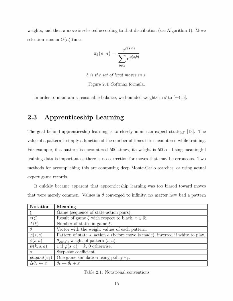
weights, and then a move is selected according to that distribution (see Algorithm 1). Move
selection runs in O(n) time.
πθ(s, a) =eφ(s,a)
∑
b∈seφ(s,b)
b is the set of legal moves in s.
Figure 2.4: Softmax formula.
In order to maintain a reasonable balance, we bounded weights in θ to [−4, 5].
2.3 Apprenticeship Learning
The goal behind apprenticeship learning is to closely mimic an expert strategy [13]. The
value of a pattern is simply a function of the number of times it is encountered while training.
For example, if a pattern is encountered 500 times, its weight is 500α. Using meaningful
training data is important as there is no correction for moves that may be erroneous. Two
methods for accomplishing this are computing deep Monte-Carlo searches, or using actual
expert game records.
It quickly became apparent that apprenticeship learning was too biased toward moves
that were merely common. Values in θ converged to infinity, no matter how bad a pattern
Notation Meaningξ Game (sequence of state-action pairs).z(ξ) Result of game ξ with respect to black, z ∈ R.T (ξ) Number of states in game ξ.θ Vector with the weight values of each pattern.ϕ(s, a) Pattern of state s, action a (before move is made), inverted if white to play.φ(s, a) θϕ(s,a), weight of pattern (s, a).ψ(k, s, a) 1 if ϕ(s, a) = k, 0 otherwise.α Step-size coefficient.playout(πθ) One game simulation using policy πθ.∆θk ← x θk ← θk + x
Table 2.1: Notational conventions
15

Algorithm 1 Random Move via Softmax Policysum← 0for all k ∈ legal moves doPk ← eφ(s,a)
sum← sum+ Pk
end forif sum = 0 then
return PASSend ifsum← sum ∗ Uniform random number in [0, 1)for all k ∈ legal moves do
if sum <= 0 thenreturn k
end ifsum← sum− Pk
end for
was for a given position. For example, endgame patterns on the edge of the board gained
very high weights, as they appear frequently during that point of the game. However, when
there are many legal positions above the second line of the board, edge plays are usually not
important. Therefore it seemed necessary to mitigate this bias.
We addressed this by introducing a simple notion of error. For each move chosen, its
pattern is incremented by α+. For each move not chosen from the same position, the
corresponding pattern is incremented by a negative value, α−. We also used Rprop, or
Resilient Backpropagation, to help compensate for error. For each round of training, each
pattern accumulates an update value that will be applied to θ. Rprop scales this update
value based on its sign change from the last update. If signs are the same, the update value
is multiplied by η+. If signs differ, the update value is multiplied by η−. These values are
1.2 and 0.5 respectively, as given by the author of Rprop [12]. See Algorithm 2 for details.
The values for α+ and α− depend on the number of training sets and the πθ function. It
is important that they do not converge out of reasonable bounds too quickly.
Apprenticeship learning proved to have slightly weaker play over a purely random policy,
although this was not unexpected. It often resulted in policies that were strong on their
own, for example, achieving 80% win rates in simulations against a purely random player.
16

Algorithm 2 Apprenticeship Learning
Old← ∅New ← ∅for all ξ ∈ expert games doP ← ∅for t = 1 to T (ξ) doNewϕ(st,at) ← α+
P ← P⋃
ϕ(st, at)for all b ∈ legal moves from st where b 6= t doNewϕ(st,b) ← α−
P ← P⋃
ϕ(st, b)end for
end forfor all k ∈ P do
if sign(Newk) = Oldk thenθk ← θk +Newk · η+
elseθk ← θk +Newk · η−
end ifOldk ← sign(Newk)
end forend for
With UCT, however, it often chose moves with good local shape but extremely poor global
influence.
2.4 Policy Gradient Reinforcement Learning
Policy gradient reinforcement learning attempts to optimize the raw strength of individual
moves in order to maximize the expected cumulative reward of a game [13]. Similar to
apprenticeship learning, an expert set of state-action pairs is used for training. A single
random simulation is generated from each training set. If the simulation result matches the
game result, all patterns generated in the simulation receive a higher preference. Otherwise,
they receive a lower preference. Like apprenticeship learning, we used Rprop to balance the
step size when updating weights. See Algorithm 3 for details.
Reinforcement learning was a noted improvement over apprenticeship learning and purely
17

Algorithm 3 Policy Gradient Reinforcement Learning
for n = 1 to N dos1 ← random state ∈ expert setξ ← playout(πθ) from s1
for t = 1 to T (ξ) do
∆θϕ(st,at) ← αz(s1)N
end forend for
random play. The variance in pattern weights was much smaller, lending to less deterministic
move selection (that is, there was less over-training).
2.5 Policy Gradient Simulation Balancing
Policy Gradient Simulation Balancing attempts to compensate for the error between V ∗
and V . Similar to the prior algorithms, it uses an expert training set of state-action pairs.
For each state-action pair, weights are updated as follows. First, M simulations are run to
produce estimate result estimate V . Next, N playouts against policy πθ are simulated, a
vector of deltas accumulates from the patterns encountered. Finally, θ is updated from the
vector of deltas, adjusting for the error (V ∗ − V ).
This means the weights are adjusted based on whether black needs to win more or less
frequently, to minimize the expected error. For example, if a game is won by white, but
playouts result in black wins, it means that the weights must be adjusted so black wins less.
See Algorithm 4 for details.
Policy gradient simulation balancing was about as strong as apprenticeship learning.
Though it converged to some good pattern distributions, it had poor global play and weighted
edge moves too low to have proper end-game responses.
18

Algorithm 4 Policy Gradient Simulation Balancing
for s1 ∈ training set doV ← 0for i = 1 to M doξ ← playout(πθ) from s1
V ← V + z(ξ)M
end forg ← 0for j = 1 to N doξ ← playout(πθ) from s1
for t = 1 to T (ξ) do
∆gϕ(st,at) ← z(ξ)NT
end forend forfor all k ∈ g do
∆θk ← α(V ∗(s1)− V )gk
end forend for
2.6 Two Step Simulation Balancing
Two Step Simulation Balancing is the second algorithm to balance overall error. The expert
training set of state-action pairs is used again. For each entry in the training set, all legal
moves two plies deep are computed. The πθ and V ∗ values for these moves are used to update
the delta vector. Once again, θ is updated using the delta vector, with compensation for
the original (V ∗ − V ). For this algorithm, V ∗ is computed using either reasonably accurate
estimates (for example, GNU Go’s heuristic evaluator), or deep Monte Carlo searches. See
Algorithm 5 for details.
Two Step Simulation Balancing grows massively complex as the board size increases. The
accuracy and simplicity of estimating a game score is vastly different between 5x5 Go (which
is completely solved), 9x9 Go, and 19x19 Go. Additionally the usefulness of a two-ply search
decreases as the board size increases. Thus, we found this algorithm to perform the weakest
compared to a purely random policy, given its computational complexity and dubious easy
applicability to 9x9 Go.
19

Algorithm 5 Two Step Simulation Balancing
for n = 1 to N doV ← 0g ← 0s1 ← random state ∈ expert setfor all a1 ∈ legal moves from s1 dos2 ← play a1 in s1
for all a2 ∈ legal moves from s2 dos3 ← play a2 in s2
p← π(s1, a1)π(s2, a2)V ← V + pV ∗(s3)∆gϕ(s1,a1) ← pV ∗(s3)∆gϕ(s2,a2) ← pV ∗(s3)
end forend forfor all k ∈ g do
∆θk ← α(V ∗(s1)− V )gk
end forend for
2.7 Development
For testing these algorithms, the Library of Effective Go Routines (libEGO) was used.
libEGO was ideal because of its minimalistic design, good code coverage density, good per-
formance, and open source license. It also supported GTP, a text protocol designed for
communication between Go clients. Its UCT implementation is described in Figure 1.6.
Implementing the softmax policy required careful attention to optimization, as it was
critical that playouts were as fast as possible. Given that a UCT invocation could result in
hundreds of thousands of simulations, even a small increase in per-playout time could result
in a noticeable difference. Luckily, the fact that there were only 216 (48) possible patterns
meant that each pattern could be represented in a 16-bit integer. This was small enough
to index patterns in a vector of 216 (65,536) elements, which used less than a megabyte of
memory to store θ. To express patterns as 16-bit integers, each intersection is encoded in
two bits, and the intersections together form a bitmap. The bit encoding (for speed and
convenience) used the same values that libEGO stored for board locations: 0 for a black
20

stone, 1 for a white stone, 2 for an empty intersection, and 3 for an edge (see Figure 2.5 for
an example).
1 0 20 22 2 1
Pattern on left, to bitboard on right.
= 0110101000100001b=0x6A21
Figure 2.5: Converting a pattern to a 16-bit integer.
The softmax policy itself was implemented according to Algorithm 1. Deducing the
pattern at a given vertex was reasonably fast thanks to libEGO’s efficient representation of
the board grid (a vector of integers), and amounted to only a handful of memory loads and
bit shifts. Additionally, the ex values were pre-computed for θ. Despite this, the algorithm
was inherently O(n) (where n is the number of legal moves), whereas the purely random
policy in libEGO was O(1). On an 2.4GHz Intel Core 2 Duo, the original random policy
ran around 28,570 simulations per second (35µs per playout), whereas the softmax policy
only managed around 3,500 per second (285µs per playout). This was an unfortunate but
unavoidable 12X decrease in performance.
Although it is possible to use uniformly weighted patterns to achieve a purely random
playout policy, it is important to note that in our implementation this is semantically different
from the libEGO default. For speed, the set of legal moves is taken to be the set of empty
intersections, but not every intersection is actually a legal move. libEGO handles this in
its playout abstraction by attempting to play the move the policy selects, and then calling
an error callback if the move is bad. If the move is bad it asks for a new vertex. The
default functionality is to simply select the next adjacent vertex. This method belied the
stochasticity implicit in “purely random,” and so we modified our move selection algorithm
to account for this. The updated version is three functions, in Algorithm 6.
21

Algorithm 6 Move Selection via Softmax Policy, 2
PrepareForMove():∀k ∈ legal moves, Pk ← eφ(s,a)
Sum←∑
k Pk
GenerateMove():if Sum = 0 then
return PASSs← Sum * Uniform random number in [0, 1)for all k ∈ legal moves do
if s <= 0 thenreturn k
s← s− Pk
end for
MarkBadMove(k):Sum← Sum− Pk
Pk ← 0
All possible symmetries are precomputed for each pattern when training begins. Given
the convenient storage of patterns as integers, rotating and flipping is just a matter of
bitshifting, though this is a one-time expense regardless. When θ needs to be updated, all
versions of a pattern are updated to receive the sum of those patterns. Special care is taken
to ensure that patterns are not encountered twice during this process; a secondary vector
shadows which patterns have been seen. To avoid excessive clearing, this array stores a
generation number for each pattern, and each “flattening” session changes the generation
number.
Other tools were used to assist in heavy-lifting. Levente Kocsis provided source code
for parsing SGF files, the de-facto text format for storing Go records. GNU Go was used
to compute V ∗ for two step simulation balancing. GoGui’s “twogtp” program was used to
playtest libEGO against GNU Go for experimentation. For additional information about
these tools, see Appendix A.
22

Chapter 3
Experiments
3.1 Setup
Each algorithm was tested with a series of benchmarks, each with a tradeoff between accuracy
and time. From least to most accurate, and likewise, fastest to slowest:
Move Guessing: Probability of πθ(s, a) correctly predicting the next move
of a random point in an expert game.
Result Guessing: Probability of playout(πθ) correctly predicting the result
of a random point in an expert game.
Playout Winrate: Win rate of playout(πθ) against libEGO’s original ran-
dom policy.
libEGO Winrate: Win rate of UCT with πθ against libEGO’s original ran-
dom policy.
GNU Go Winrate: Win rate of UCT with πθ against a reference expert
program (GNU Go 3.8).
All training data was gathered from the NNGS (No-Name Go Server) game archives [1].
Only 9x9 games between two different, human opponents, both ranked at 12-kyu or higher,
were used. Computer program records were not interesting, since often they play very
23
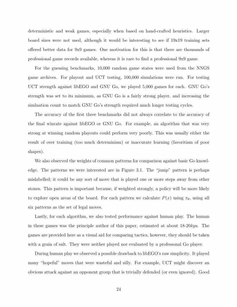
deterministic and weak games, especially when based on hand-crafted heuristics. Larger
board sizes were not used, although it would be interesting to see if 19x19 training sets
offered better data for 9x9 games. One motivation for this is that there are thousands of
professional game records available, whereas it is rare to find a professional 9x9 game.
For the guessing benchmarks, 10,000 random game states were used from the NNGS
game archives. For playout and UCT testing, 100,000 simulations were run. For testing
UCT strength against libEGO and GNU Go, we played 5,000 games for each. GNU Go’s
strength was set to its minimum, as GNU Go is a fairly strong player, and increasing the
simluation count to match GNU Go’s strength required much longer testing cycles.
The accuracy of the first three benchmarks did not always correlate to the accuracy of
the final winrate against libEGO or GNU Go. For example, an algorithm that was very
strong at winning random playouts could perform very poorly. This was usually either the
result of over training (too much determinism) or inaccurate learning (favoritism of poor
shapes).
We also observed the weights of common patterns for comparison against basic Go knowl-
edge. The patterns we were interested are in Figure 3.1. The “jump” pattern is perhaps
mislabelled; it could be any sort of move that is played one or more steps away from other
stones. This pattern is important because, if weighted strongly, a policy will be more likely
to explore open areas of the board. For each pattern we calculate P (x) using πθ, using all
six patterns as the set of legal moves.
Lastly, for each algorithm, we also tested performance against human play. The human
in these games was the principle author of this paper, estimated at about 18-20kyu. The
games are provided here as a visual aid for comparing tactics, however, they should be taken
with a grain of salt. They were neither played nor evaluated by a professonal Go player.
During human play we observed a possible drawback to libEGO’s raw simplicity. It played
many “hopeful” moves that were wasteful and silly. For example, UCT might discover an
obvious attack against an opponent group that is trivially defended (or even ignored). Good
24

Go players typically do not play such moves as they waste potential ko threats. It is likely
that our UCT playout count was not deep enough to discover more meaningful moves on
the board, or that UCT decided it was more valuable to risk a mistake on behalf of the
opponent.
(a) Hane, strong (b) Empty triangle,weak
(c) Suicide, weak
(d) Jump, strong (e) Cut #1, strong (f) Cut #2, strong
Figure 3.1: Interesting test patterns.
25

3.2 libEGO Uniform Random
The default libEGO algorithm is to select a move according to a uniformly random distribu-
tion. If the selected move is illegal, adjacent empty intersections are tried until a valid one
is found. If no intersections are free, libEGO passes.
Move Guessing: 1.6%Result Guessing: 52.8%Playout Winrate: 46.6%libEGO Winrate: 48.4%GNU Go Winrate: 46.2%
Table 3.1: libEGO Uniform Random Experiments.
The results in Table 3.1 are the baseline for observing whether an algorithm performs
better or worse than the libEGO default. Of particular note is the game record in Figure 3.2.
Using this policy, the computer barely managed to make a shape capable of living. Despite
numerous mistakes on behalf of the human player, the computer resigned. While it took
advantage of poor moves such as 19 , it made serious mistakes. For example, 40 should
have been at 41 , and other algorithms in this paper indeed discovered the better move.
1
2
3
45
67
8
910 11
12
13
1415
16
17
18 19
20
21
22
23
24
25
26 27
28
29
30 31
32
33
34
35
36 37
38
39
40
41
42
43
44
45
46
47
48 4950
51
5253
54
55 56
57
58
Computer (W) resigns to human (B).
Figure 3.2: Human versus uniform random policy.
26

3.3 Apprenticeship Learning
As mentioned earlier, apprenticeship learning suffers from over-training; each pattern has
the potential to converge to∞ or −∞. Although the algorithm was tweaked to compensate
for this, it was still highly dependent on the number of training sets. To slow growth we
empirically tested various α+ and α− values, using both simple playouts and fast UCT games
(10,000 simulations) against a purely random player.
Move Guessing: 1.5%Result Guessing: 53.3%Playout Winrate: 73.8%libEGO Winrate: 40.2%GNU Go Winrate: 42.6%
Table 3.2: Apprenticeship learning results.
!!"
#$"
#!"
%$"
%!"
&$"
&!"
'$($$$$$)" '$($$$$$!" '$($$$$)" '$($$$$!" '$($$$)" '$($$$!"
!"#
$%&'$%()*+,'-"./(,&'0$&/1&.,2'
34'1*4&51"&.,'
$($$!"
$($)"
$($*"
$($+"
$($,"
36'1*4&51"&.,'
Figure 3.3: Simple playout winrates for some apprenticeship coefficients.
As demonstrated in Figure 3.3, single playouts against a random player became much
stronger. Contrasted with Figure 3.4, however, none of the results were good. We chose
α+ = 0.005, α− = −0.0005 for the full suite of tests in Table 3.2.
Apprenticeship learning seemed to arrive at some reasonable values for our experimental
patterns. The empty triangle and suicide were strongly disfavored. Cut #2 and hane did not
27

!"
#"
$"
%"
&"
'!"
'#"
'$"
(!)!!!!!'" (!)!!!!!*" (!)!!!!'" (!)!!!!*" (!)!!!'" (!)!!!*"
!"#$%&'(%&)%*++%,-./$%
01%2&3/42"/#(%
!)!!*"
!)!'"
!)!#"
!)+"
!)$"
03%2&3/42"/#(%
Figure 3.4: Winrates against random player for some apprenticeship coefficients.
receive extraordinarily high weights. The jump pattern, unfortunately, received an extreme
disfavor. This was most likely the result of over-training; since this pattern occurs in many
positions, but is not always played, our error compensation considered it bad.
To test this theory we altered the algorithm slightly. Previously we had applied α− to
patterns resulting from unchosen moves. We changed this to exclude patterns matching the
originally chosen pattern. This resulted in much more sensible values. Not unexpectedly,
this also resulted in much stronger local play, quickly discovering severe attacks on weak
shapes. However its global play weakened, as it became too focused on local eye shape,
and overall performed worse. Nonetheless this “fixed” version of the algorithm seems more
promising and warrants further exploration.
Pattern P (x) old P (x) newHane 22.2% 14.2%Empty Triangle 0.4% 0.7%Suicide 7.3% 0.3%Jump 0.4% 42.0%Cut #1 52.2% 42.0%Cut #2 17.5% 0.8%
Table 3.3: Apprenticeship learning pattern statistics.
Figure 3.6 shows a game record of an apprenticeship-trained policy against a human.
28
!"
!#"
!##"
!###"
!####"
$%"
$&'(%"
$&')*"
$)'+)"
$)',("
$)')"
$!'*%"
$!'%*"
$!'!)"
$#'-("
$#'%"
$#'#%"
#'&)"
#'(*"
!'#%"
!'%"
!'-("
)'!)"
)'%*"
)'*%"
&')"
&',("
&'+)"
%')*"
%'(%"
,"
!"#$%&'()'*+,%&-.'/0(12'
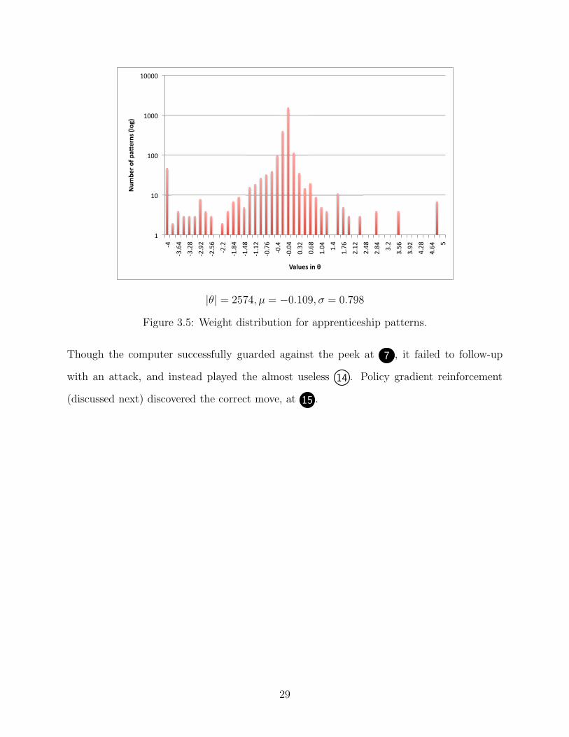
3+0"%.'4-'5'
|θ| = 2574, µ = −0.109, σ = 0.798
Figure 3.5: Weight distribution for apprenticeship patterns.
Though the computer successfully guarded against the peek at 7 , it failed to follow-up
with an attack, and instead played the almost useless 14 . Policy gradient reinforcement
(discussed next) discovered the correct move, at 15 .
29

1
2
3
4
56
7 8
9
10
11
1213
14
15
1617
18 19
2021
22
23
24
25
26
27 28
29
30 31
3233
34
35
36
37
3839
40
41
42
434445
4647
4849
50
51
52
535455
58
60
61
62
63
64
Human (B) defeats computer (W) by 5.5 points.
Figure 3.6: Human versus apprenticeship learning.
3.4 Policy Gradient Reinforcement Learning
Policy gradient reinforcement learning (PGRL) proved much more sporadic than appren-
ticeship learning. Its output was highly dependent on the ratio of αT
and the relationship
between α+ and α−. Lower values of αT
formed more concentrated, less deterministic results.
Higher values caused extreme determinism.
To demonstrate these extremeties, we experimented with three result sets using T =
100, 000: PGRLlow with α = 1, PGRLmed with α = 4, and PGRLhigh with α = 50. See
Table 3.4 for details.
PGRLlow PGRLmed PGRLhigh
Move Guessing: 2.5% 3.6% 6.0%Result Guessing: 53.0% 53.2% 53.6%Playout Winrate: 61.9% 75.6% 93.8%libEGO Winrate: 58.8% 54.2% 24.1%GNU Go Winrate: 51.0% 45.2% 34.4%
Table 3.4: Policy gradient reinforcement results.
Unfortunately as PGRL became more deterministic, it also became weaker, preferring
some odd patterns over others. This can be seen in Table 3.5. As αT
grew, the jump and cut
patterns converged to 0. Although not demonstrated here, changing the distance between
30

α+ and α− made the policy more deterministic. α+ > α− biased toward bad moves, and the
reverse relationship acted similar to PGRLhigh with a higher preference for cut #1.
Pattern P (x) PGRLlow P (x) PGRLmed P (x) PGRLhigh
Hane 18.3% 20.3% 18.4%Empty Triangle 15.2% 11.5% 0.8%Suicide 18.4% 20.8% 11.9%Jump 10.9% 5.8% 0.8%Cut #1 18.2% 19.3% 0.8%Cut #2 18.9% 22.3% 67.4%
(a) Test pattern probabilities.
PGRLlow PGRLmed PGRLhigh
µ -0.062 -0.166 -1.382σ 0.113 0.286 1.720
(b) Weight distribution in θ.
Table 3.5: Policy gradient reinforcement pattern statistics.
The sheer difference the coefficient made could be seen in human play as well. In Fig-
ure 3.7, PGRLlow played a calm, accurate game, and won by 1.5 points. Note how it cleanly
captured territory down the middle of the board. PGRLhigh, however, was hopelessly spo-
radic in Figure 3.8. Almost every move by white was a mistake, and the survival of its group
was questionable after 33 (the rest was not played out).
1
2
34
5
6 7
8
910
11
12 13
14
15
16 17
18
1920 21
22 23
24
25
26
27
28
29
30
31
32
33
Computer (W) calmly defeats human (B) by 1.5 points.
Figure 3.7: PGRLlow versus human.
31

1
2
3
4
5
6
7
8
9
10 11
12
13
14
15
17
19
20
21
22
23 24
252627
28
2930
31
32
33
34
Computer (W) has no hope of defeating human (B) here.
Figure 3.8: PGRLhigh versus human.
3.5 Policy Gradient Simulation Balancing
Policy gradient simulation balancing produced mixed and generally disappointing results.
The variables we experimented with were M (which estimates the policy winrate), N (which
gathers and updates patterns through simulation), the step-size coefficient α, and the number
of training iterations. The algorithm began yielding reasonable results with M = N = 100;
anything significantly less was too inaccurate. Tweaking the step-size, we were able to
achieve very strong playouts against the random player, upwards of 90% winrates and higher.
Unfortunately, even though pattern statistics looked promising, overall play was poor.
One reason for this was that simulation balancing highly disregarded moves along the
edge of the board. For example, a common edge pattern received a weight of −2.7, a
miniscule number for the numerator of the softmax formula. In the end game, these patterns
are critical for protecting against unwanted encroachment into territory. Many simulation
balancing games had acceptable gameplay until the end, at which point they let their groups
die by not considering simple moves. We decided to superficially address this problem by
introducing a higher lower bound (−2, from a previous −5) on final weight values.
Even with this change, simulation balancing resulted in lukewarm play. It could solve
life and death situations, but was not aggressive enough to capture territory. It spent a
32

good deal of energy making useless cuts that only strengthened opponent formations. Many
simulated games resulted in a small loss simply from a lack of aggressive opening moves.
One reason for this could be that there is no guarantee that a policy will be improved
simply by playing against itself. Although simulation balancing attempts to correct for error,
a policy can play only bad moves against itself and come to the conclusion that those moves
are good. We tested this theory by using three trials of simulation balancing. The first,
PGSB0, was trained from empty weights. The second, PGSBpgrl, was trained using the
weights from PGRLlow. Lastly, PGSBal was trained using the weights from apprenticeship
learning (the original version). All instances used 10,000 training sets and α = 1. Our
hope was that with an initial “good” set of data, simulation balancing would improve it
further. Unfortunately, as shown in Table 3.6, neither PGRL nor apprenticeship learning
was improved.
PGSB0 PGSBpgrl PGSBal
Move Guessing: 1.9% 1.7% 12.9%Result Guessing: 52.9% 52.9% 53.1%Playout Winrate: 55.4% 51.5% 67.3%libEGO Winrate: 41.4% 43.2% 16.9%GNU Go Winrate: 43.1% 41.2% 34.4%
Table 3.6: Simulation balancing results.
Pattern preferences for PGSB0 were mostly evenly distributed, with the jump gaining a
favorable advantage. PGSBpgrl and PGSBal looked fairly similar to their original weights.
Raising the α coefficient converged to a more optimal distribution. However, UCT play with
these weights was very poor.
PGSBpgrl and PGSBal suffered from poor endgame play. In Figure 3.9, 28 is a severe
mistake, prompting an immediate play from black at 29 . The computer was able to prevent
further damage, but the loss was unrecoverable and it later resigned (not shown). PGSB0
on the other hand played a better game, shown in Figure 3.10. Its play was far from flawless,
however; for example, move 8 was a wasted move, especially so early in the game. It did
catch a black mistake at 21 , but failed to follow up with a more aggressive attack.
33

Pattern P (x) PGSB0 P (x) PGSBpgrl P (x) PGSBal
Hane 16.3% 15.3% 22.5%Empty Triangle 14.8% 15.3% 1.9%Suicide 17.0% 15.7% 5.7%Jump 19.4% 23.5% 1.9%Cut #1 16.5% 15.2% 55.7%Cut #2 16.2% 15.1% 12.4%
(a) Test pattern probabilities.
PGSB0 PGSBpgrl PGSBal
µ 0.222 0.03 -0.032σ 0.064 0.035 0.605
(b) Weight distribution in θ.
Table 3.7: Simulation balancing pattern statistics.
3.6 Two Step Simulation Balancing
Two step simulation balancing resulted in weak performance. This was most likely the result
of several mitigating factors. We used GNU Go 3.8 to precompute the approximate V ∗ of
the complete two-ply depth of random positions from 1,000 games. More data points would
have been desireable, but the process was extremely expensive. An hour of computation on
one CPU resulted in only one to five training sets, and time and resources were limited.
Move Guessing: 6.5%Result Guessing: 53.3%Playout Winrate: 66.0%libEGO Winrate: 33.9%GNU Go Winrate: 27.6%
Table 3.8: Two step simulation balancing results.
We also computed V ∗ as either a win or a loss, which may have been too coarse. As the
size of a Go board increases, it is less likely that two moves from a position will significantly
change the score in a meaningful way. Furthermore, as mentioned earlier, score estimation
before the end of a game is extremely difficult in Go, and prone to gross inaccuracies. These
observations suggest that either two step simulation balancing does not scale to larger boards
well, or that V ∗ needs to be computed with finer granularity (perhaps, as a difference between
34

1
2
3
4 5
6 7
8
9
10
11
12 13
14 15
16
17
18 19
20
21
22
23
24
2526
27
28
29
Computer (W) resigns to human (B).
Figure 3.9: PGSBpgrl versus human.
1
2
3
4
5
6
7
8
9 10
111213
14
15
16 18 19
2021
22
23
24
25
26
27
28
30
3132
33
34
35
36 37
38 39
40
41
42
43
44
45
46
47
48
49
50
51
52
53
54 55
56
Computer (W) defeats human (B) by 2.5 points.
Figure 3.10: PGSB0 versus human.
expected scores).
For our results, we used α+ = 1.3 and α− = 1.6.
Two step’s poor overall play is easily seen in Figure 3.11. From the start, 4 is bad. It is
too slow a move, forming strong shape but gaining no valuable territory. The computer also
failed to solve basic life and death situations. Move 57 killed the computer’s large group
of stones; a white play at the same position would have saved it, or turned it into ko. Two
step simulation balancing seemed weak at both the local and global scope of the board.
35

Pattern P (x)Hane 13.1%Empty Triangle 2.8%Suicide 10.5%Jump 2.8%Cut #1 2.8%Cut #2 67.9%
Table 3.9: Two step simulation pattern statistics.
1
2
3
4
5
6
7
8
9
10
11
12
13
14
15
16
17
18
19
20
21 22 23
24
25
26 27
28
29
30
32
33
34
35
36
37
38
39
40
41
42
43 44
4647
48
49
50
51
52 53
54
55
56
57
Computer (W) has lost badly to human (B).
Figure 3.11: Two step simulation balancing versus human.
36

Chapter 4
Conclusions
In this project, we implemented and tested four algorithms proposed in the Monte Carlo
Simulation Balancing paper [13]. Two of these algorithms maximized the strength of indi-
vidual moves in random simulations, whereas the other two minimized the whole-game error
of random simulations. We trained these algorithms using a database of amateur 9x9 games,
using 3x3 patterns to parameterize the simulation policy. We experimented the effectiveness
of these algorithms on 9x9 Go.
The first strength algorithm, Apprenticeship Learning, learned a strong policy, but it
proved too deterministic for play with UCT. Even with superficial compensation for error,
its strength in a full game was slightly worse than purely random.
The second strength algorithm, Policy Gradient Reinforcement Learning, learned a mod-
erately strong policy with a fairly concentrated pattern distribution. With full UCT play, it
slightly outperformed a purely random policy.
The first balancing algorithm, Policy Gradient Simulation Balancing, learned a very
strong policy with a seemingly logical pattern distribution. However, its gameplay with UCT
was weaker than a purely random policy. Edge moves in particular received unnecessarily
low preferences due to their weakness in general gameplay. This caused the computer to
miss extremely important end-game tactics. While local play was otherwise strong, moves
37

in the opening had poor global perspective, and stones often ended up clumped together.
The second balancing algorithm, Two Step Simulation Balancing, performed the weakest,
significantly worse than a purely random policy. While it learned a strong simulation policy,
it was too deterministic and biased toward poor pattern distributions. The original authors
tested Two Step Balancing on a 5x5 board [13]. The nature of the algorithm suggested that
it probably did not scale to larger boards. It required computing a score estimate which was
both computationally expensive and inaccurate. While it was possible that we did not have
enough training data (due to time constraints), it was also likely that the two-ply depth of
a game was not enough to infer a meaningful score change.
!"
#!"
$!"
%!"
&!"
'!"
(!"
)!"
*!"
+,-./01" 234"+056"7-89/:" ;<2";/"
!"#$%&'()*+(
,--.#'#&(
+056"7-89/:"
=>>568?@6ABC>"
76C8D/5@6:681"
EC:0,-?/8"F-,-8@C8G"
4H/"E16>"F-,-8@C8G"
Figure 4.1: Final comparison of all algorithms.
We also observed that all four algorithms were capable of highly strong policies, achieving
up to 95% winrate or higher against purely random simulations. This did not necessarily
mean, however, that the policy was playing good moves. In fact, it usually meant the
policy was too deterministic, and playout winrates this high tended to fare poorly with
UCT. Relatedly, we did not attempt to try any policy other than the softmax policy. It
38

is possible that this was not a good probability function given the distribution of pattern
weights resulting from our training data.
As a final observation, the unpromising results of our experiments may reflect the sheer
complexity of Go. Our training sets and computational power were limited, and this might
not have been sufficient enough for the reinforcement and balancing algorithms to converge
to a good solution. On the other hand, the domain of larger Go boards may simply be too
vast and complex to produce meaningful results.
39

Appendix A
Development Notes
For producing this paper, we used the following tools:
• LATEX for typesetting (TeXShop as an editor)
• Microsoft Excel 2008 for producing EPS graphs
• OmniGraffle for producing flow charts
• psgo LATEX package for drawing Go diagrams
• GoGui for exporting large diagrams to LATEX
As mentioned earlier, we used libEGO as a codebase for implementing the softmax policy
and training algorithms. We also used GNU Go 3.8 as a reference expert program, and to
evaluate board positions for Two Step Simulation Balancing.
The layout of our source code tarball is as follows:
• libego - Contains our modified libEGO source code, as well as our implementation of
all algorithms in this paper.
• sgfparser - Modified SGF (game record) parser originally given by Levente Kocsis.
• paper - The LATEX source code to this paper.
40
All source code was tested on GCC 4.2, on OS X 10.5, and on Debian Linux (x86 64).
The SGF parser is built via “make rand db” and accepts the following command line
arguments:
• sgflist=[file] ; Required. File containing a list of SGF files.
• mode=[0,1] ; Required. Mode 0 outputs random game states for move and result
guessing. Mode 1 outputs a compact representation of games that can be used for
training.
• rank=[value] ; Optional. “value” must be a valid rank, such as 12kyu. Games below
this rank are excluded.
• maxgames=[value] ; Required. Maximum number of SGF files to parse.
All data from “rand db” is written to standard out.
We modified libEGO’s parameters such that the first parameter must be either “random”
(meaning the original, purely random playout policy) or the path to a file containing a set
of patterns and their weights, which invokes the softmax policy.
Lastly, the following is a brief command line documentation for all algorithm training
and testing tools we developed.
apprentice <training file> <alpha+> <alpha->
Apprenticeship Learning. Results are written to standard out.
pgrad_rprop <training file> <nsimulations> <alpha+> <alpha->
Policy Gradient Reinforcement Learning. Results are written to standard out.
The nsimulations parameter specifies how many training sets to run.
simbal <training file> <M> <N> <nsimulations> <alpha+> <alpha-> [prev]
Policy Gradient Simulation Balancing. Results are written to standard out.
41

The nsimulations parameter specifies how many training sets to run.
The optional prev parameter specifies a file with initial weights to use.
build_twostep <training file> <nsimulations> <outfolder> <prefix>
Builds score estimation database for Two Step Simulation Balancing.
The nsimulations parameter specifies how many game states to compute.
The outfolder parameter specifies where to store output files.
The prefix parameter specifies a prefix for output file names.
Note: "gnugo" must be in PATH.
Bug: child process is not terminated properly on premature exit.
twostep <folder> <prefix> <alpha+> <alpha->
Two Step Simulation Balancing. Results are written to standard out.
The outfolder parameter specifies where to store output files.
The prefix parameter specifies a prefix for output file names.
ptop <pattern file>
Displays the 5 highest and lowest weighted patterns.
Displays sum, average, variance, and standard deviation for weights.
Displays P(x) for six patterns in our artificial distribution.
simpolicy <count> <black> <white>
Plays simulated games between two policies and returns the black winrate.
The count parameter is the number of simulations to run.
The black and white parameters are policies to use. Each must either be
"random" or a file containing a pattern database.
fastsim <database> <fast|slow|bench> [policy]
42

Performs a benchmark on a policy and prints the result.
The database parameter must be a file from mode 0 of "rand_db".
The "fast" variant is move guessing.
The "slow" variant is result guessing.
The "bench" variant benchmarks the policy for time.
The policy parameter must either be empty (random) or a pattern file.
playtestXk.py <black> <white> <ngames> <prefix> <strength>
Plays full games between two GTP programs, using gogui-twogtp.
Results and SGF files are written to files.
The black and white parameters must either be "gnugo", or a policy
parameter that libEGO would take on the command line.
The ngames parameter specifies the number of games to play.
The prefix parameter specifies a common prefix for file output.
The strength parameter changes libEGO if it is used. "default"
specifies the "ego_opt" program, anything else is "ego_<strenght>".
grid.py <policy> <start> <end> <prefix> <strength> <ngames> <opponent>
Submits (end-start) games to Condor using condor_submit.
All results are (overwritten) to the "sresults" folder in the working
directory. File names have the start, end, and prefix parameters.
Game count per grid job is specified via ngames.
The policy parameter is the black player for playtestXk.py.
The prefix and strength parameters are passed to playtestXk.py.
The opponent is the white player for playtestXk.py.
stats.pl <prefix>
43

Finds all grid results submitted with a certain prefix in the
"sresults" folder, and displays the winrate of black.
44

Bibliography
[1] Guido Adam. NNGS archive data?, Apr 21, 2006. Online posting. Computer-Go
mailing list. Mar 17 2009 <http://www.computer-go.org/pipermail/computer-go/2006-
April/005343.html>.
[2] Victor Allis. Searching for Solutions in Games and Artificial Intelligence. PhD thesis,
University of Limburg, Maastricht, 1994. ISBN 9090074880.
[3] Peter Auer, Nicolo Cesa-Bianchi, and Paul Fischer. Finite-time analysis of the Multi-
armed Bandit Problem. Machine Learning, 47(2-3):235–256, 2002.
[4] Bruno Bouzy. Associating shallow and selective tree search with Monte Carlo for 9x9
Go. Fourth International Conference on Computers and Games, 2004.
[5] Bernd Brugmann. Monte Carlo Go. Technical report, Max-Planck-Institute of Physics,
Oct 9 1993.
[6] Ken Chen and Zhixing Chen. Static analysis of life and death in the game of Go. Inf.
Sci. Inf. Comput. Sci., 121(1-2):113–134, 1999.
[7] Remi Coulom. Efficient Selectivity and Backup Operators in Monte-Carlo Tree Search.
Fifth International Conference on Computers and Games, pages 72–83, 2006.
[8] Chris Garlock. Computer Beats Pro at U.S. Go Congress. American Go Association
News, Aug 7, 2008.
45

[9] Sylvain Gelly et al. Modification of UCT with Patterns in Monte-Carlo Go. INRIA,
Nov 2006.
[10] Levente Kocsis and Csaba Szepesvari. Bandit based Monte-Carlo Planning. European
Conference on Machine Learning, pages 282–293, 2006.
[11] Dylan Loeb McClain. Once Again, Machine Beats Human Champion at Chess. The
New York Times, Dec 5, 2006.
[12] Martin Riedmiller. Rprop - Description and Implementation Details. Technical report,
University of Karlsruhe, Jan 1994.
[13] David Silver and Gerald Tesauro. Monte-Carlo Simulation Balancing. The Learning
Workshop, 2009.
46