montage: a grid portal and software toolkit for science ... · pdf fileint. j. computational...

Int. J. Computational Science and Engineering, Vol 4, No.2, 2009 1

Montage: a grid portal and

software toolkit for science-grade

astronomical image mosaicking

Joseph C. Jacob*, Daniel S. Katz Jet Propulsion Laboratory, California Institute of Technology,

Pasadena, CA 91109-8099

E-mail: {Joseph.C.Jacob*, Daniel.S.Katz}@jpl.nasa.gov

*Corresponding author

G. Bruce Berriman, John Good, Anastasia C. Laity Infrared Processing and Analysis Center, California Institute of Technology

Pasadena, CA 91125

E-mail: {gbb, jcg, laity}@ipac.caltech.edu

Ewa Deelman, Carl Kesselman, Gurmeet Singh, Mei-Hui Su USC Information Sciences Institute,

Marina del Rey, CA 90292

E-mail: {deelman, carl, gurmeet, mei}@isi.edu

Thomas A. Prince, Roy Williams California Institute of Technology

Pasadena, CA 91125

E-mail: [email protected], [email protected]

Abstract: Montage is a portable software toolkit for constructing custom, science-grade mosaics by composing multiple astronomical images. The mosaics constructed by Montage preserve the astrometry (position) and photometry (intensity) of the sources in the input images. The mosaic to be constructed is specified by the user in terms of a set of parameters, including dataset and wavelength to be used, location and size on the sky, coordinate system and projection, and spatial sampling rate. Many astronomical datasets are massive, and are stored in distributed archives that are, in most cases, remote with respect to the available computational resources. Montage can be run on both single- and multi-processor computers, including clusters and grids. Standard grid tools are used to run Montage in the case where the data or computers used to construct a mosaic are located remotely on the Internet. This paper describes the architecture, algorithms, and usage of Montage as both a software toolkit and as a grid portal. Timing results are provided to show how Montage performance scales with number of processors on a cluster computer. In addition, we compare the performance of two methods of running Montage in parallel on a grid.

Keywords: astronomy; image mosaic; grid portal, TeraGrid, virtual observatory.

Biographical notes: Joseph C. Jacob has been a researcher at the Jet Propulsion Laboratory, California Institute of Technology, since he completed his PhD in computer engineering at Cornell University in 1996. His research interests are in the areas of parallel and distributed computing, image processing and scientific visualization.

Daniel S. Katz received his PhD in Electrical Engineering from Northwestern University in 1994. He is currently a Principal member of the Information Systems and Computer Science Staff at JPL. His current research interest include numerical methods, algorithms, and programming applied to supercomputing, parallel computing, and cluster computing; and fault-tolerant computing.

G. Bruce Berriman received his PhD in Astronomy from the California Institute of Technology. He is currently the project manager of NASA's Infrared Science Archive,

2 J. C. JACOB, ET AL.

based at the Infrared Processing and Analysis Center at the California Institute of Technology. His current research interests include searching for the very coolest stars (“brown dwarfs”) and the development of on-request Grid services for astronomy.

John C. Good received his PhD in Astronomy from the University of Massachusetts in 1983. He is currently the project architect for NASA's Infrared Science Archive, based at the Infrared Processing and Analysis Center at the California Institute of Technology and has been heavily involved for many years in distributed information systems development for astronomy.

Anastasia Clower Laity received a Bachelor's Degree in Physics and Astronomy from Pomona College in 2000. She has been at the Infrared Processing and Analysis Center (IPAC) since 2002, working primarily as a software developer and system administrator on several data archiving projects.

Ewa Deelman is a Research Team Leader at the Center for Grid Technologies at the USC Information Sciences Institute and an Assistant Research Professor at the USC Computer Science Department. Dr. Deelman's research interests include the design and exploration of collaborative scientific environments based on Grid technologies, with particular emphasis on workflow management as well as the management of large amounts of data and metadata. Dr. Deelman received her PhD from Rensselaer Polytechnic Institute in Computer Science in 1997 in the area of parallel discrete event simulation.

Carl Kesselman is the Director of the Center for Grid Technologies at the Information Sciences Institute at the University of Southern California. He is an ISI Fellow and a Research Professor of Computer Science at the University of Southern California. Dr. Kesselman received his PhD in Computer Science at the University of California at Los Angeles and an honorary PhD from the University of Amsterdam.

Gurmeet Singh received his MS in Computer Science from University of Southern California in 2003. He is currently a graduate student in the Computer Science department at USC. His current research interests include resource provisioning and task scheduling aspects of grid computing.

Mei-Hui Su received her BS in Electrical Engineering and Computer Sciences from University of California, Berkeley. She currently is a system programmer at the Center for Grid Technologies at the USC Information Sciences Institute. Her interests include Grid technology, distributed and parallel computing.

Thomas A. Prince is a Professor of Physics at the California Institute of Technology. He received his PhD from the University of Chicago. Currently he is serving as the Chief Scientist of the NASA Jet Propulsion Laboratory. His research includes gravitational wave astronomy and computational astronomy.

Roy Williams received his PhD in Physics from the California Institute of Technology. He is currently a senior scientist at the Caltech Center for Advanced Computing Research. His research interests include science gateways for the grid, multi-plane analysis of astronomical surveys, and real-time astronomy.

Int. J. Computational Science and Engineering, Vol 4, No.2, 2009 1

1 INTRODUCTION

Wide-area imaging surveys have assumed fundamental

importance in astronomy. They are being used to address

such fundamental issues as the structure and organization of

galaxies in space and the dynamical history of our galaxy.

One of the most powerful probes of the structure and

evolution of astrophysical sources is their behavior with

wavelength, but this power has yet to be fully realized in the

analysis of astrophysical images because survey results are

published in widely varying coordinates, map projections,

sizes and spatial resolutions. Moreover, the spatial extent of

many astrophysical sources is much greater than that of

individual images. Astronomy therefore needs a general

image mosaic engine that will deliver image mosaics of

arbitrary size in any common coordinate system, in any map

projection and at any spatial sampling rate. The Montage

project (Berriman et al., 2002; 2004) has developed this

capability as a scalable, portable toolkit that can be used by

astronomers on their desktops for science analysis,

integrated into project and mission pipelines, or run on

computing grids to support large-scale product generation,

mission planning and quality assurance. Montage produces

science-grade mosaics that preserve the photometric

(intensity) and astrometric (location) fidelity of the sources

in the input images.

Sky survey data are stored in distributed archives that are

often remote with respect to the available computational

resources. Therefore, state-of-the-art computational grid

technologies are a key element of the Montage portal

architecture. The Montage project is deploying a science-

grade custom mosaic service on the Distributed Terascale

Facility or TeraGrid (http://www.teragrid.org/). TeraGrid is

a distributed infrastructure, sponsored by the National

Science Foundation (NSF), and is capable of 20 teraflops

peak performance, with 1 petabyte of data storage, and 40

gigabits per second of network connectivity between the

multiple sites.

The National Virtual Observatory (NVO, http://www.us-

vo.org/) and International Virtual Observatory Alliance

(http://www.ivoa.net/) aim to establish the infrastructure

necessary to locate, retrieve, and analyze astronomical data

hosted in archives around the world. Science application

portals can easily take advantage of this infrastructure by

complying with the protocols for data search and retrieval

that are being proposed and standardized by these virtual

observatory projects. Montage is an example of one such

science application portal being developed for the NVO.

Astronomical images are almost universally stored in

Flexible Image Transport System (FITS) format

(http://fits.gsfc.nasa.gov/). The FITS format encapsulates

the image data with a meta-data header containing keyword-

value pairs that, at a minimum, describe the image

dimensions and how the pixels map to the sky. The World

Coordinate System (WCS) specifies image-to-sky

coordinate transformations for a number of different

coordinate systems and projections useful in astronomy

(Greisen and Calabretta, 2002). Montage uses FITS for

both the input and output data format and WCS for

specifying coordinates and projections.

Montage is designed to be applicable to a wide range of

astronomical image data, and has been carefully tested on

images captured by three prominent sky surveys spanning

multiple wavelengths, the Two Micron All Sky Survey,

2MASS (http://www.ipac.caltech.edu/2mass/), the Digitized

Palomar Observatory Sky Survey, DPOSS

(http://www.astro.caltech.edu/~george/dposs/), and the

Sloan Digital Sky Survey (SDSS). 2MASS has roughly 10

terabytes of images and catalogues (tabulated data that

quantifies key attributes of selected celestial objects found

in the images), covering nearly the entire sky at 1-arc-

second sampling in three near-infrared wavelengths.

DPOSS has roughly 3 terabytes of images, covering nearly

the entire northern sky in one near-infrared wavelength and

two visible wavelengths. The SDSS fourth data release

(DR4) contains roughly 7.4 terabytes of images and

catalogues covering 6,670 square degrees of the Northern

sky in five visible wavelengths.

Two previously published papers provide background on

Montage. The first described Montage as part of the

architecture of the National Virtual Observatory (Berriman

et al., 2002), and the second described some of the initial

grid results of Montage (Berriman et al., 2004). In addition,

a book chapter and a paper (Katz et al., 2005a; 2005b)

provide highlights of the results reported in this paper. We

extend these previous publications by providing additional

details about the Montage algorithms, architectures, and

usage.


In this paper, we describe the modular Montage toolkit, the

algorithms employed, and two strategies that have been

used to implement an operational service on the TeraGrid,

accessible through a web portal. The remainder of the paper

is organized as follows. Section 2 describes how Montage

is designed as a modular toolkit. Section 3 describes the

algorithms employed in Montage. Section 4 describes the

architecture of the Montage TeraGrid portal. Two strategies

for running Montage on the TeraGrid are described in

Sections 5 and 6, with a performance comparison in Section

7. A summary is provided in Section 8.

2 MONTAGE COMPONENTS

Montage’s goal is to provide astronomers with software for

the computation of custom science-grade image mosaics in

FITS format. Custom refers to user specification of mosaic

parameters, including WCS projection, coordinate system,

mosaic size, image rotation, and spatial sampling rate.

Science-grade mosaics preserve the calibration and

astrometric (spatial) fidelity of the input images.

There are three steps to building a mosaic with Montage:

Reprojection of input images to a common

projection, coordinate system, and spatial scale,

Modeling of background radiation in images to

rectify them to a common flux scale and

background level, thereby minimizing the inter-

image differences, and

Coaddition of reprojected, background-rectified

images into a final mosaic.

Montage accomplishes these tasks in independent,

portable, ANSI C modules. This approach controls testing

and maintenance costs, and provides flexibility to users.

They can, for example, use Montage simply to reproject sets

of images and co-register them on the sky, implement a

custom background removal algorithm, or define another

processing flow through custom scripts. Table 1 describes

the core computational Montage modules and Figure 1

illustrates how they may be used to produce a mosaic.

Three usage scenarios for Montage are as follows: the

modules listed in Table 1 may be run as stand-alone

programs; the executive programs listed in the table (i.e.,

mProjExec, mDiffExec, mFitExec, and mBgExec) may be

used to process multiple input images either sequentially or

in parallel via MPI; or the grid portal described in Section 4

may be used to process a mosaic in parallel on a

computational grid. The modular design of Montage

permits the same set of core compute modules to be used

regardless of the computational environment being used.

3 MONTAGE ALGORITHMS

Table 1 The core design components of Montage

Component Description

Mosaic Engine Components

mImgtbl Extract geometry information from a set of FITS headers and create a metadata table

from it.

mProject Reproject a FITS image.

mProjExec A simple executive that runs mProject for each image in an image metadata table.

mAdd Coadd the reprojected images to produce an

output mosaic.

Background Rectification Components

mOverlaps Analyze an image metadata table to determine

which images overlap on the sky.

mDiff Perform a simple image difference between a

pair of overlapping images. This is meant for use on reprojected images where the pixels

already line up exactly.

mDiffExec Run mDiff on all the overlap pairs identified by mOverlaps.

mFitplane Fit a plane (excluding outlier pixels) to an

image. Meant for use on the difference

images generated by mDiff.

mFitExec Run mFitplane on all the mOverlaps pairs.

Creates a table of image-to-image difference

parameters.

mBgModel Modeling/fitting program which uses the image-to-image difference parameter table to

interactively determine a set of corrections to apply to each image to achieve a "best" global

fit.

mBackground Remove a background from a single image (a

planar correction has proven to be adequate for the images we have dealt with).

mBgExec Run mBackground on all the images in the

metadata table

Figure 1 The high-level design of Montage.

MONTAGE: A GRID PORTAL AND SOFTWARE TOOLKIT FOR SCIENCE-GRADE ASTRONOMICAL IMAGE MOSAICKING 5

As described in Section 2, Montage constructs a mosaic

through separate modules for image reprojection,

background rectification, and coaddition. This section

describes the main algorithms used in these modules.

3.1 General image reprojection

The first step in mosaic construction is to reproject each

input image to the spatial scale, coordinate system, and

projection of the output mosaic. Image reprojection

involves the redistribution of information from a set of input

pixels to a set of output pixels. For astronomical data, the

input pixels represent the total energy received from an area

on the sky, and it is critical to preserve this information

when redistributed into output pixels. Also, in astronomy it

is important to preserve the positional (astrometric)

accuracy of the energy distribution, so common techniques

such as adding all the energy from an input pixel to the

“nearest” output pixel are inadequate. Instead, we must

redistribute input pixel energy to the output based on the

exact overlap of these pixels, possibly even using a

weighting function across the pixels based on the point

spread function for the original instrument.

The most common approach to determining pixel overlap

is to project the input pixel into the output Cartesian space.

This works well for some projection transformations but is

difficult for others. One example of a difficult

transformation is the Aitoff projection, commonly used in

astronomy, where locations at the edge of an image

correspond to undefined locations in pixel space. For

Montage, we have decided instead to project both input and

output pixels onto the celestial sphere. Since all such

“forward” projections are well defined, the rest of the

problem reduces to calculating the area of overlap of two

convex polygons on a sphere (with no further consideration

of the projections). The issue of handling reprojections thus

becomes a problem of classical spherical trigonometry.

General algorithms exist for determining the overlap of

polygons in Cartesian space (O’Rourke, 1998). We have

modified this approach for use in spherical coordinates to

determine the intersection polygon on the sphere (a convex

hull) and applied Girard's Theorem, which gives the area of

a spherical triangle based on the interior angles, to calculate

the polygon’s area.

The result is that for any two overlapping pixels, we can

determine the area of the sky from the input pixel that

contributes energy to the output pixel. This provides a

mechanism for accurately distributing input energy to

output pixels and a natural weighting mechanism when

combining overlapping images.

Our approach implicitly assumes that the polygon defining

a single pixel can be approximated by the set of great circle

segments connecting the pixel’s corners. Since even the

largest pixels in any realistic image are on the order of a

degree across, the nonlinearities along a pixel edge are

insignificant. Furthermore, the only affect this would have

would be to the astrometric accuracy of the energy location

information and it would amount to a very small fraction

(typically less that 0.01) of the size of a pixel. Total energy

is still conserved.

http://math.rice.edu/~pcmi/sphere


3.2 Rapid image reprojection

Image reprojection is by far the most compute-intensive part

of the processing because, in its general form, mapping

from input image to output mosaic coordinates is done in

two steps. First, input image coordinates are mapped to sky

coordinates (i.e., right ascension and declination, analogous

to longitude and latitude on the Earth). Second, those sky

coordinates are mapped to output image coordinates. All of

the mappings from one projection to another are compute-

intensive, but some require more costly trigonometric

operations than others and a few require even more costly

iterative algorithms. The first public release of Montage

applied this two-step process to the corners of the input

pixels in order to map the flux from input image space to

output space. Because the time required for this process

stood as a serious obstacle to using Montage for large-scale

image mosaics of the sky, a novel algorithm that is about 30

times faster was devised for the second code release.

The new much faster algorithm uses a set of linear

equations (though not a linear transform) to transform

directly from input pixel coordinates to output pixel

coordinates. This alternate approach is limited to cases

where both the input and output projections are “tangent

plane” type (gnomonic, orthographic, etc.), but since these

projections are by far the most common, it is appropriate to

treat them as a special case.

This “plane-to-plane” approach is based on a library

developed at the Spitzer Science Center (Makovoz and

Khan, 2004). When both images are tangent plane, the

geometry of the system can be viewed as in Figure 2, where

a pair of gnomonic projection planes intersects the

coordinate sphere. A single line connects the center of the

sphere, the projected point on the first plane and the

projected point on the second plane. This geometric

relationship results in transformation equations between the

two planar coordinate systems that require no trigonometry

or extended polynomial terms. As a consequence, the

transform is a factor of thirty or more faster than using the

normal spherical projection formulae.

A bonus to the plane-to-plane approach is that the

computation of pixel overlap is much easier, involving only

clipping constraints of the projected input pixel polygon in

the output pixel space.

This approach excludes many commonly-used projections

such as “Cartesian” and “zenithal equidistant,” and is

essentially limited to small areas of few square degrees.

Processing of all-sky images, as is almost always the case

with projections such as Aitoff, generally requires the

slower plane-to-sky-to-plane approach.

There is, however, a technique that can be used for images

of high resolution and relatively small extent (up to a few

degrees on the sky). Rather than use the given image

projection, we can often approximate it with a very high

degree of accuracy with a “distorted” Gnomonic projection.

In this case, the pixel locations are “distorted” by small

distances relative to the plane used in the image projection

formulae. A distorted space is one in which the pixel

locations are slightly offset from the locations on the plane

used by the projection formulae, as happens when detectors

are slightly misshapen, for instance. This distortion is

modelled by pixel-space polynomial correction terms that

are stored as parameters in the image FITS header.

While this approach was developed to deal with physical

distortions caused by telescope and instrumental effects, it is

also applicable to Montage in augmenting the plane-to-

plane reprojection. Over a small, well-behaved region, most

projections can be approximated by a Gnomonic (TAN)

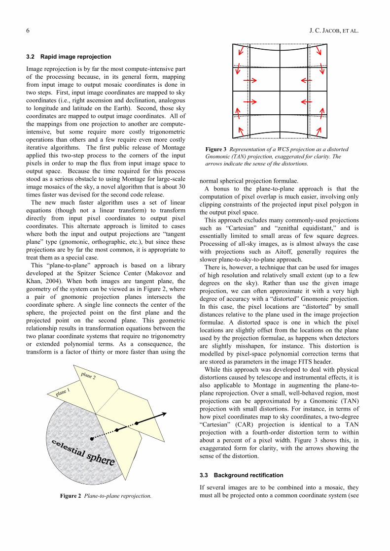
projection with small distortions. For instance, in terms of

how pixel coordinates map to sky coordinates, a two-degree

“Cartesian” (CAR) projection is identical to a TAN

projection with a fourth-order distortion term to within

about a percent of a pixel width. Figure 3 shows this, in

exaggerated form for clarity, with the arrows showing the

sense of the distortion.

3.3 Background rectification

If several images are to be combined into a mosaic, they

must all be projected onto a common coordinate system (see

Figure 2 Plane-to-plane reprojection.

Figure 3 Representation of a WCS projection as a distorted

Gnomonic (TAN) projection, exaggerated for clarity. The

arrows indicate the sense of the distortions.


above) and then any discrepancies in brightness or

background must be removed, as illustrated in Figure 4. Our

assumption is that the input images are all calibrated to an

absolute energy scale (i.e., brightnesses are absolute and

should not be modified) and that any discrepancies between

the images are due to variations in their background levels

that are terrestrial or instrumental in origin.

The Montage background rectification algorithm is based

on the assumption that terrestrial and instrumental

backgrounds can be described by simple linear functions or

surfaces (e.g., slopes and offsets). Stated more generally,

we assume that the “non-sky” background has very little

energy in any but the lowest spatial frequencies. If this not

the case, it is unlikely that any generalized background

matching algorithm will be able distinguish between “sky”

and rapidly varying “background”; background removal

would then require an approach that depends on a detailed

knowledge of an individual data set.

Given a set of overlapping images, characterization of the

overlap differences is key to determining how each image

should be adjusted before combining them. We consider

each image individually with respect to its neighbours.

Specifically, we determine the areas of overlap between

each image and its neighbours, and use the complete set of

overlap pixels in a least-squares fit to determine how each

image should be adjusted (e.g., what gradient and offset

should be added) to bring it best in line with its neighbours.

In practice, we adjust the image by half this optimal

amount, since all the neighbors are also being analyzed and

adjusted and we want to avoid ringing. After doing this for

all the images, we iterate (currently for a fixed number of

iterations, though a convergence criteria could be used).

The final effect is to have subtracted a low-frequency

(currently a gradient and offset) background from each

image such that the cumulative image-to-image differences

are minimized. To speed the computation and minimize

memory usage, we approximate the gradient and offset

values by a planar surface fit to the overlap area difference

images rather than perform a least squares fit using all of the

overlap pixels.

3.4 Coaddition

In the reprojection algorithm (described above), each input

pixel’s energy contribution to an output pixel is added to

that pixel, weighted by the sky area of the overlap. In

addition, a cumulative sum of these sky area contributions is

kept for the output pixels (called an “area” image). When

combining multiple overlapping images, these area images

provide a natural weighting function; the output pixel value

is simply the area-weighted average of the pixels being

combined.

Such images are in practice very flat (with only slight

slopes due to the image projection) since the cumulative

effect is that each output pixel is covered by the same

amount of input area, regardless of the pattern of coverage.

The only real variation occurs at the edges of the area

covered, since there an output pixel may be only partially

covered by input pixels.

The limitations of available memory have been simply

overcome in coaddition by reading the reprojected images

one line at a time from files that reside on disk. Assuming

that a single row of the output file does not fill the memory,

the only limitation on file size is that imposed by the file

system. Indeed, images of many gigabytes have thus far

been built with the new software. For each output line,

mAdd determines which input files will be contributing

pixel values, and opens only those files. Each contributing

pixel value is read from the flux and area coverage files, and

the value of each of these pixels is stored in an array until

all contributing pixels have been read for the corresponding

output row. This array constitutes a “stack” of input pixel

Figure 4 A Montage mosaic before (left) and after (right) background rectification.


values; a corresponding stack of area coverage values is also

preserved. The contents of the output row are then

calculated one output pixel (i.e., one input stack) at a time,

by averaging the flux values from the stack.

Different algorithms to perform this average can be

trivially inserted at this point in the program. Montage

currently supports mean and median coaddition, with or

without weighting by area. The mean algorithm (the default)

accumulates flux values contributing to each output pixel,

and then scales them by the total area coverage for that

pixel. The median algorithm ignores any pixels whose area

coverage falls below a specific threshold, and then

calculates the median flux value from the remainder.

If there are no area files, then the algorithm gives equal

weight to all pixels. This is valuable for science data sets

where the images are already projected into the same pixel

space (e.g., MSX). An extension of the algorithm to support

outlier rejection is planned for a future release.

3.5 Drizzle

The Space Telescope Science Institute (STScI) has

developed a method for the linear reconstruction of an

image from under-sampled, dithered data. The algorithm is

known as “drizzling,” or more formally as Variable-Pixel

Linear Reconstruction (Fruchter and Hook, 2002). Montage

provides drizzle as an option in the image reprojection. In

this algorithm, pixels in the original input images are

mapped onto the output mosaic as usual, except the pixel is

first “shrunken” by a user-defined amount. This is

particularly easy to do in Montage. Since the Montage

algorithm projects the corners of each pixel onto the sky, we

implement drizzle by simply using a different set of corners

in the interior of the original pixel. In other words, the flux

is modelled as all coming from a box centered on the

original pixel but smaller by the drizzle factor.

4 MONTAGE GRID PORTAL ARCHITECTURE

The basic user interface to Montage is implemented as a

web portal. In this portal, the user selects a number of input

parameters for the mosaicking job, such as the centre and

size of the region of interest, the source of the data to be

mosaicked, and some identification such as an email

address. Once this information is entered, the user assumes

that the mosaic will be computed, and she will be notified of

the completion via an email message containing a URL

where the mosaic can be retrieved.

Behind the scenes, a number of things have to happen.

First, a set of compute resources needs to be chosen. Here,

we will assume that this is a cluster with processors that

have access to a shared file system. Second, the input data

files and executable code needs to be moved to these

resources. Third, the modules need to be executed in the

right order. In general, this might involve moving

intermediate files from one set of resources to another, but

the previous assumption makes this file movement

unnecessary. Fourth, the output mosaic and some status

information need to be moved to a location accessible to the

user. Fifth and finally, the user must be notified of the job

completion and the location of the output files.

The Montage TeraGrid portal includes components

distributed across computers at the Jet Propulsion

Laboratory (JPL), Infrared Processing and Analysis Center

(IPAC), USC Information Sciences Institute (ISI), and the

TeraGrid, as illustrated in Figure 5. Note that the

description here applies to 2MASS mosaics, but can be

easily extended to DPOSS and SDSS images as well. The

portal is comprised of the following five main components,

each having a client and server as described below: (i) User

Portal, (ii) Abstract Workflow Service, (iii) 2MASS Image

List Service, (iv) Grid Scheduling and Execution Service,

and (v) User Notification Service.

Figure 5 The Montage TeraGrid portal architecture.


This design exploits the parallelization inherent in the

Montage architecture. The Montage grid portal is flexible

enough to run a mosaic job on a number of different cluster

and grid computing environments, including Condor pools

and TeraGrid clusters. We have demonstrated processing

on both a single cluster configuration and on multiple

clusters at different sites having no shared disk storage.

4.1 User portal

Users on the Internet submit mosaic requests by filling in

a simple web form with parameters that describe the mosaic

to be constructed, including an object name or location,

mosaic size, coordinate system, projection, and spatial

sampling rate. After request submission, the remainder of

the data access and mosaic processing is fully automated

with no user intervention.

The server side of the user portal includes a CGI program

that receives the user input via the web server, checks that

all values are valid, and stores the validated requests to disk

for later processing. A separate daemon program with no

direct connection to the web server runs continuously to

process incoming mosaic requests. The processing for a

request is done in two main steps:

1. Call the abstract workflow service client code

2. Call the grid scheduling and execution service client

code and pass to it the output from the abstract

workflow service client code

4.2 Abstract workflow service

The abstract workflow service takes as input a celestial

object name or location on the sky and a mosaic size and

returns a zip archive file containing the abstract workflow as

a directed acyclic graph (DAG) in XML and a number of

input files needed at various stages of the Montage mosaic

processing. The abstract workflow specifies the jobs and

files to be encountered during the mosaic processing, and

the dependencies between the jobs. These dependencies are

used to determine which jobs can be run in parallel on

multiprocessor systems. A pictorial representation of an

abstract workflow for computing a mosaic from three input

images is shown in Figure 6.

4.3 2MASS image list service

The 2MASS Image List Service takes as input a celestial

object name or location on the sky (which must be specified

as a single argument string), and a mosaic size. The

2MASS images that intersect the specified location on the

sky are returned in a table, with columns that include the

filenames and other attributes associated with the images.

4.4 Grid scheduling and execution service

The Grid Scheduling and Execution Service takes as input

the abstract workflow, and all of the input files needed to

Figure 6 Example abstract workflow.


construct the mosaic. The service authenticates users using

grid security credentials stored in a MyProxy server

(Novotny et al., 2001), schedules the job on the grid using

Pegasus (Deelman et al., 2002; 2003; 2004), and then

executes the job using Condor DAGMan (Frey et al., 2001).

Section 6 describes how this is done in more detail.

4.5 User notification service

The last step in the grid processing is to notify the user

with the URL where the mosaic may be downloaded. This

notification is done by a remote user notification service at

IPAC so that a new notification mechanism can be used

later without having to modify the Grid Scheduling and

Execution Service. Currently the user notification is done

with a simple email, but a later version will use the Request

Object Management Environment (ROME), being

developed separately for the National Virtual Observatory.

ROME will extend our portal with more sophisticated job

monitoring, query, and notification capabilities.

5 GRID-ENABLING MONTAGE VIA MPI

PARALLELIZATION

The first method of running Montage on a grid is to use

grid-accessible clusters, such as the TeraGrid. This is very

similar to traditional, non-grid parallelization. By use of

MPI, the Message Passing Interface (Snir et al., 1996), the

executives (mProjExec, mDiffExec, mFitExec, mBgExec,

mAddExec) and mAdd can be run on multiple processors.

The Atlasmaker (Williams et al., 2003) project previously

developed an MPI version of mProject, but it was not

closely coupled to the released Montage code, and therefore

has not continued to work with current Montage releases.

The current MPI versions of the Montage modules are

generated from the same source code as the single-processor

modules by preprocessing directives.

The structure of the executives are similar to each other, in

that each has some initialization that involves determining a

list of files on which a module will be run, a loop in which

the module is actually called for each file, and some

finalization work that includes reporting on the results of the

module runs. The executives, therefore, are parallelized

straightforwardly, with all processes of a given executive

being identical to each other. All the initialization is

duplicated by all of the processes. A line is added at the

start of the main loop, so that each process only calls the

sub-module if the remainder of the loop count divided by

the number of processes equals the MPI rank (a logical

identifier of an MPI process). All processes then participate

in global sums to find the total statistics of how many sub-

modules succeeded, failed, etc., as each process keeps track

of its own statistics. After the global sums, only the process

with rank 0 prints the global statistics.

mAdd writes to the output mosaic one line at a time,

reading from its input files as needed. The sequential mAdd

writes the FITS header information into the output file

before starting the loop on output lines. In the parallel

mAdd, only the process with rank 0 writes the FITS header

information, then it closes the file. Each process then

carefully seeks and writes to the correct part of the output

file. Each process is assigned a unique subset of the rows of

the mosaic to write, so there is no danger of one process

overwriting the work of another. While the executives were

written to divide the main loop operations in a round-robin

fashion, it makes more sense to parallelize the main mAdd

loop by blocks, since it is likely that a given row of the

output file will depend on the same input files as the

previous row, and this can reduce the amount of input I/O

for a given process.

Note that there are two modules that can be used to build

the final output mosaic, mAdd and mAddExec, and both can

be parallelized as discussed in the previous two paragraphs.

At this time, we have just run one or the other, but it would

be possible to combine them in a single run.

A set of system tests is available from the Montage web

site. These tests, which consist of shell scripts that call the

various Montage modules in series, were designed for the

single-processor version of Montage. The MPI version of

Montage is run similarly, by changing the appropriate lines

of the shell script, for example, from:

mProjExec arg1 arg2 ...

to:

mpirun -np N mProjExecMPI arg1 arg2 ...

No other changes are needed. If this is run on a queue

system, a set of processors is reserved for the job. Some

parts of the job, such as mImgtbl, only use one processor,

and other parts, such as mProjExecMPI, use all the

processors. Overall, most of the processors are in use most

of the time. There is a small bit of overhead here in

launching multiple MPI jobs on the same set of processors.

One might change the shell script into a parallel program,

perhaps written in C or Python, to avoid this overhead, but

this has not been done for Montage.

The processing part of this approach is not very different

from what might be done on a cluster that is not part of a

grid. In fact, one might choose to run the MPI version of

Montage on a local cluster by logging into the local cluster,

transferring the input data to that machine, submitting a job

that runs the shell script to the queuing mechanism, and

finally, after the job has run, retrieving the output mosaic.

Indeed, this is how the MPI code discussed in this paper was

run and measured. The discussion of how this code could

be used in a portal is believed to be correct, but has not been

implemented and tested.

6 GRID-ENABLING MONTAGE WITH PEGASUS

Pegasus (Planning for Execution in Grids), developed as

part of the GriPhyN Virtual Data (http://www.griphyn.org/),


is a framework that enables the mapping of complex

workflows onto distributed resources such as the grid. In

particular, Pegasus maps an “abstract workflow” to a

“concrete workflow” that can be executed on the grid using

a variety of computational platforms, including single hosts,

Condor pools, compute clusters, and the TeraGrid.

An abstract workflow describes a computation in terms of

logical transformations and data without identifying the

resources needed to execute it. The Montage abstract

workflow consists of the various application components

shown in Figure 6. The nodes represent the logical

transformations such as mProject, mDiff and others. The

edges represent the data dependencies between the

transformations. For example, mConcatFit requires all the

files generated by all the previous mFitplane steps.

6.1 Mapping application workflows

Pegasus maps an abstract workflow description to a

concrete, executable form after consulting various grid

information services to find suitable resources, the data that

is used in the workflow, and the necessary software. In

addition to specifying computation on grid resources, this

concrete, executable workflow also has data transfer nodes

(for both stage-in and stage-out of data), data registration

nodes that can update various catalogues on the grid (for

example, RLS), and nodes that can stage-in binaries.

Pegasus finds any input data referenced in the workflow

by querying the Globus Replica Location Service (RLS),

assuming that data may be replicated across the grid

(Chervenak et al., 2002). After Pegasus derives new data

products, it can register them into the RLS as well.

Pegasus finds the programs needed to execute a workflow,

including their environment setup requirements, by

querying the Transformation Catalogue (TC) (Deelman et

al., 2001). These executable programs may be distributed

across several systems.

Pegasus queries the Globus Monitoring and Discovery

Service (MDS) to find the available compute resources and

their characteristics such as the load, the scheduler queue

length, and available disk space (Czajkowski et al., 2001).

Additionally, the MDS is used to find information about the

location of the GridFTP servers (Allcock et al., 2002) that

can perform data movement, job managers (Czajkowski et

al., 2001) that can schedule jobs on the remote sites, storage

locations, where data can be pre-staged, shared execution

directories, the RLS into which new data can be registered,

site-wide environment variables, etc.

The information from the TC is combined with the MDS

information to make scheduling decisions, with the goal of

scheduling a computation close to the data needed for it.

One other optimization that Pegasus performs is to reuse

those workflow data products that already exist and are

registered into the RLS, thereby eliminating redundant

computation. As a result, some components from the

abstract workflow may not appear in the concrete workflow.

6.2 Workflow execution

The concrete workflow produced by Pegasus is in the form

of submit files that are given to DAGMan and Condor-G for

execution. The submit files indicate the operations to be

performed on given remote systems and dependencies, to be

enforced by DAGMAN, which dictate the order in which

the operations need to be performed.

In case of job failure, DAGMan can retry a job a given

number of times. If that fails, DAGMan generates a rescue

workflow that can be potentially modified and resubmitted

at a later time. Job retry is useful for applications that are

sensitive to environment or infrastructure instability. The

rescue workflow is useful in cases where the failure was due

to lack of disk space that can be reclaimed or in cases where

totally new resources need to be assigned for execution.

Obviously, it is not always beneficial to map and execute an

entire workflow at once, because resource availability may

change over time. Therefore, Pegasus also has the

capability to map and then execute (using DAGMan) one or

more portions of a workflow (Deelman et al., 2004).

7 COMPARISON OF GRID EXECUTION STRATEGIES

AND PERFORMANCE

Here we discuss the advantages and disadvantages of each

of the two approaches (MPI and Pegasus) we took to

running Montage on the grid. We quantify the performance

of the two approaches and describe how they differ.

7.1 Benchmark problem and system

In order to test the two approaches to grid-enabling

Montage, we chose a sample problem that could be

computed on a single processor in a reasonable time as a

benchmark. The results in this paper involve this

benchmark, unless otherwise stated.

The benchmark problem generates a mosaic of 2MASS

data from a 6 x 6 degree region at M16. This requires 1,254

input 2MASS images, each about 0.5 megapixel, for a total

of about 657 megapixels (about 5 GB with 64 bits/pixel

double precision floating point data). The output is a 3.7

GB FITS (Flexible Image Transport System) file with a

21,600 x 21,600 pixel data segment, and 64 bits/pixel

double precision floating point data. The output data is a

little smaller than the input data size because there is some

overlap between neighboring input images. For the timing

results reported in this section, the input data had been pre-

staged to a local disk on the compute cluster.

Results in this paper are measured on the “Phase 2”

TeraGrid cluster at the National Center for Supercomputing

Applications (NCSA), unless otherwise mentioned. This

cluster has (at the time of this experiment) 887 nodes, each

with dual Itanium 2 processors with at least 4 GB of

memory. 256 of the nodes have 1.3 GHz processors, and

the other 631 nodes have 1.5 GHz processors. The timing

tests reported in this paper used the 1.5 GHz processors. The

network between nodes is Myrinet and the operating system


is SuSE Linux. Disk I/O is to a 24 TB General Parallel File

System (GPFS). Jobs are scheduled on the system using

Portable Batch System (PBS) and the queue wait time is not

included in the execution times since that is heavily

dependent on machine load from other users.

Figure 6 shows the processing steps for the benchmark

problem. There are two types of parallelism: simple file-

based parallelism, and more complex module-based

parallelism. Examples of file-based parallelism are the

mProject modules, each of which runs independently on a

single file. mAddExec, which is used to build an output

mosaic in tiles, falls into this category as well, as once all

the background-rectified files have been built, each output

tile may be constructed independently, except for I/O

contention. The second type of parallelism can be seen in

mAdd, where any number of processors can work together

to build a single output mosaic. This module has been

parallelized over blocks of rows of the output, but the

parallel processes need to be choreographed to write the

single output file correctly. The results in this paper are for

the serial version of mAdd, where each output tile is

constructed by a single processor.

7.2 Starting the job

In both the MPI and Pegasus implementations, the user can

choose from various sets of compute resources. For MPI,

the user must specify a single set of processors that share a

file system. For Pegasus, this restriction is removed since it

can automatically transfer files between systems. Thus,

Pegasus is clearly more general. Here, we compare

performance on a single set of processors on the TeraGrid

cluster, described previously as the benchmark system.

7.3 Data and code stage-in

In either approach, the need for both data and code stage-in

is similar. The Pegasus approach has clear advantages, in

that the RLS and Transformation Catalogue can be used to

locate the input data and proper executables for a given

machine, and can stage the code and data to an appropriate

location. In the MPI approach, the user must know where

the executable code is, which is not a problem when the

portal executes the code, as it then is the job of the portal

creator. Data reuse can also be accomplished with a local

cache, though this is not as general as the use of RLS.

In any event, input data will sometimes need to be retrieved

from an archive. In the initial version of the portal

discussed in this paper, we use the 2MASS list service at

IPAC, but a future implementation will use the proposed

standard Simple Image Access (SIA) protocol

(http://www.ivoa.net/Documents/latest/SIA.html), which

returns a table listing the files (URLs) that can be retrieved.

7.4 Building the mosaic

With the MPI approach, the portal generates a shell script

and a job to run it is submitted to the queue. Each command

in the script is either a sequential or parallel command to

run a step of the mosaic processing. The script will have

some queue delay, and then will start executing. Once it

starts, it runs until it finishes with no additional queue

delays. The script does not contain any detail on the actual

data files, just the directories. The sequential commands in

the script examine the data directories and instruct the

parallel jobs about the actual file names.

The Pegasus approach differs in that the initial work is

more complex, but the work done on the compute nodes is

much simpler. For reasons of efficiency, a pool of

processors is allocated from the parallel machine by use of

the queue. Once this pool is available, Condor-Glidein

(http://www.cs.wisc.edu/condor/glidein/) is used to

associate this pool with an existing Condor pool. Condor

DAGMan then can fill the pool and keep it as full as

possible until all the jobs have been run. The decision about

what needs to be run and in what order is made by the

portal, where the mDAG module builds the abstract DAG,

and Pegasus then builds the concrete DAG.

Because the queuing delays are one-time delays for both

methods, we do not discuss them any further. The elements

for which we discuss timings below are the sequential and

parallel jobs for the MPI approach, and the mDAG, Pegasus,

and compute modules for the Pegasus approach.

7.5 MPI timing results

The timing results of the MPI version of Montage are

shown in Figure 7. The total times shown in this figure

include both the parallel modules (the times for which are

also shown in the figure) and the sequential modules (the

times for which are not shown in the figure, but are

relatively small).

The end-to-end runs of Montage involved running the

modules in this order: mImgtbl, mProjExec, mImgtbl,

mOverlaps, mDiffExec, mFitExec, mBgModel, mBgExec,

mImgtbl, mAddExec.

Figure 7 Performance of MPI version of Montage building a

6 x 6 degree mosaic.


MPI parallelization reduces the one processor time of 453

minutes down to 23.5 minutes on 64 processors, for a

speedup of 19. Note that with the exception of some small

initialization and finalization code, all of the parallel code is

non-sequential. The main reason the parallel modules fail to

scale linearly as the number of processors is increased is

I/O. On a system with better parallel I/O, one would expect

to obtain better speedups; the situation where the amount of

work is too small for the number of processors has not been

reached, nor has the Amdahl’s law limit been reached.

Note that there is certainly some variability inherent in

these timings, due to the activity of other users on the

cluster. For example, the time to run a serial module like

mImgtbl shouldn’t vary with number of processors, but the

measured results vary from 0.7 to 1.4 minutes. Also, the

time for mDiffExec on 64 processors is fairly different from

that on 16 and 32 processors. This appears to be caused by

I/O load from other jobs running simultaneously with

Montage. Additionally, since some of the modules’ timings

are increasing as the number of processors is increased, one

would actually run the module on the number of processors

that minimizes the timing. For example, mBgExec on this

machine should only be run on 16 processors, no matter

how many are used for the other modules.

These timings are probably close to the best that can be

achieved on a single cluster, and can be thought of as a

lower bound on any parallel implementation, including any

grid implementation. However, there are numerous

limitations to this implementation, including that a single

pool of processors with shared access to a common file

system is required, and that any single failure of a module or

submodule will cause the entire job to fail, at least from that

point forward. The Pegasus approach described in Section 6

can overcome these limitations.

7.6 Pegasus timing results

When using remote grid resources for the execution of the

concrete workflow, there is a non-negligible overhead

involved in acquiring resources and scheduling the

computation over them. In order to reduce this overhead,

Pegasus can aggregate the nodes in the concrete workflow

into clusters so that the remote resources can be utilized

more efficiently. The benefit of clustering is that the

scheduling overhead (from Condor-G, DAGMan and

remote schedulers) is incurred only once for each cluster. In

the following results we cluster the nodes in the workflow

within a workflow level (or workflow depth). In the case of

Montage, the mProject jobs are within a single level, mDiff

jobs are in another level, and so on. Clustering can be done

dynamically based on the estimated run time of the jobs in

the workflow and the processor availability.

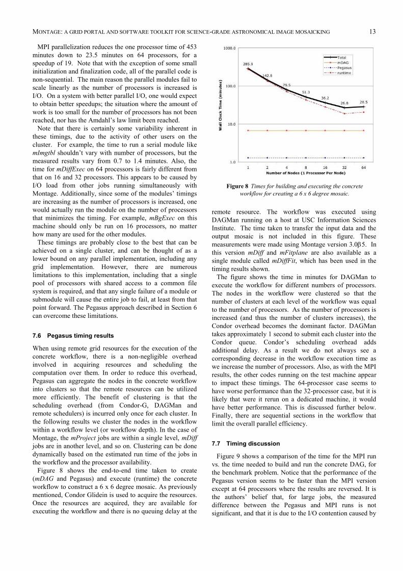
Figure 8 shows the end-to-end time taken to create

(mDAG and Pegasus) and execute (runtime) the concrete

workflow to construct a 6 x 6 degree mosaic. As previously

mentioned, Condor Glidein is used to acquire the resources.

Once the resources are acquired, they are available for

executing the workflow and there is no queuing delay at the

remote resource. The workflow was executed using

DAGMan running on a host at USC Information Sciences

Institute. The time taken to transfer the input data and the

output mosaic is not included in this figure. These

measurements were made using Montage version 3.05. In

this version mDiff and mFitplane are also available as a

single module called mDiffFit, which has been used in the

timing results shown.

The figure shows the time in minutes for DAGMan to

execute the workflow for different numbers of processors.

The nodes in the workflow were clustered so that the

number of clusters at each level of the workflow was equal

to the number of processors. As the number of processors is

increased (and thus the number of clusters increases), the

Condor overhead becomes the dominant factor. DAGMan

takes approximately 1 second to submit each cluster into the

Condor queue. Condor’s scheduling overhead adds

additional delay. As a result we do not always see a

corresponding decrease in the workflow execution time as

we increase the number of processors. Also, as with the MPI

results, the other codes running on the test machine appear

to impact these timings. The 64-processor case seems to

have worse performance than the 32-processor case, but it is

likely that were it rerun on a dedicated machine, it would

have better performance. This is discussed further below.

Finally, there are sequential sections in the workflow that

limit the overall parallel efficiency.

7.7 Timing discussion

Figure 9 shows a comparison of the time for the MPI run

vs. the time needed to build and run the concrete DAG, for

the benchmark problem. Notice that the performance of the

Pegasus version seems to be faster than the MPI version

except at 64 processors where the results are reversed. It is

the authors’ belief that, for large jobs, the measured

difference between the Pegasus and MPI runs is not

significant, and that it is due to the I/O contention caused by

Figure 8 Times for building and executing the concrete

workflow for creating a 6 x 6 degree mosaic.


other jobs running on the test platform during these runs. A

dedicated system would serve to mitigate these differences.

To examine some of these timings in more detail, we

study the work needed to create a 1-degree square mosaic

on 8 processors, as shown in Figure 10. The first difference

is that mImgtbl is run three times in the MPI code vs. only

once in the Pegasus code, where mDAG and Pegasus are run

in advance instead of the first two mImgtbl runs. This is

because the DAG is built in advance for Pegasus, but for

MPI, the inputs are built on the fly from the files created by

previous modules. Second, one MPI module starts

immediately after the previous module finishes, while the

Pegasus modules have a gap where nothing is running on

the TeraGrid. This is the overhead imposed by DAGMan, as

mentioned above. Third, the MPI code is almost 3 times

faster for this small problem.

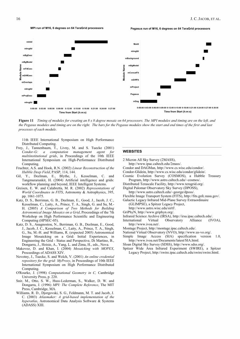
If we examine a larger problem, such as the 64 processor

runs that create the 36 square degree test problem, as seen in

Figure 11, we see some differences. First, the overall times

are now comparable. Second, in the Pegasus case, the gaps

between the modules are generally not noticeable, except

between mProject and mDiffFit and between mBgModel and

mBackground. Since the bars show the range of time of 64

processes now, some of the gaps are just hidden, while some

are truly insignificant. Finally, in the Pegasus case, the

mDAG and Pegasus times are substantial, but the mAdd time

is much shorter than in the MPI case. Again, this is just a

difference between the two implementations: mDAG allows

the individual mAdd processes to open only the relevant

files in the Pegasus case, whereas in the MPI case, the

region of coverage is not known in advance, so all mAdd

instances must open all files. Many are then closed

immediately, if they are determined to not intersect the

output tile. The I/O overhead in the MPI case is much

larger, but the startup time is much shorter.

It is possible that a larger number of experiments run on a

large dedicated machine would further illuminate the

differences in performance between the MPI and Pegasus

approaches, but even on the heavily-loaded TeraGrid cluster

at NCSA, it is clear that there is no performance difference

that outweighs the other advantages of the Pegasus

approach, such as fault tolerance and the ability to use

multiple machines for a single large job.

7.8 Finishing the job

Once the output mosaic has been built, it must be made

available to the user, and the user must be notified of this

availability. The Montage portal currently transfers the

mosaic from the compute processors to the portal, and

emails the user. In the case of Pegasus, the mosaic is also

registered in RLS. The time required to transfer the mosaic

and to notify the user are common to both the Pegasus and

MPI approaches, and thus are not discussed here.

8 CONCLUSION

Montage was written as a very general set of modules to

permit a user to generate astronomical image mosaics. A

Montage mosaic is a single image that is built from multiple

smaller images and preserves the photometric and

astrometric accuracy of the input images. Montage includes

modules that are used to reproject images to common

coordinates, calculate overlaps between images, calculate

coefficients to permit backgrounds of overlap regions to be

matched, modify images based on those coefficients, and

coadd images using a variety of methods of handling

multiple pixels in the same output space.

The Montage modules can be run on a single processor

computer using a simple shell script. Because this approach

can take a long time for a large mosaic, alternatives to make

use of the grid have been developed. The first alternative,

using MPI versions of the computation-intensive modules,

performs well but is somewhat limited. A second

alternative, using Pegasus and other grid tools, is more

general and allows for execution on a variety of platforms

without requiring a change in the underlying code base, and

appears to have real-world performance comparable to that

of the MPI approach for reasonably large problems.

Pegasus allows various scheduling techniques to be used to

optimize the concrete workflow for a particular execution

platform. Other benefits of Pegasus include

opportunistically making best use of available resources

through dynamic workflow mapping, and taking advantage

of pre-existing intermediate data products.

The Montage software, user guide and user support

system are available on the project web site at

http://montage.ipac.caltech.edu/. Montage has been used

by a number of NASA projects for science data product

generation, quality assurance, mission planning, and

outreach. These projects include: two Spitzer Legacy

Projects, SWIRE (Spitzer Wide Area Infrared Experiment,

http://swire.ipac.caltech.edu/swire/swire.html) and

GLIMPSE (Galactic Legacy Infrared Mid-Plane Survey

Extraordinaire, http://www.astro.wisc.edu/sirtf/); NASA’s

Figure 9 Times for building and executing the concrete workflow

for creating a 6 x 6 degree mosaic.


Infrared Science Archive, IRSA

(http://irsa.ipac.caltech.edu/); and the Hubble Treasury

Program, the COSMOS Cosmic Evolution Survey

(http://www.astro.caltech.edu/~cosmos/).

ACKNOWLEDGEMENT

Montage is funded by NASA's Earth Science Technology

Office, Computational Technologies (ESTO-CT) Project,

under Cooperative Agreement Number NCC5-626 between

NASA and the California Institute of Technology. Pegasus

is supported by NSF under grants ITR-0086044 (GriPhyN)

and ITR AST0122449 (NVO).

Part of this research was carried out at the Jet Propulsion

Laboratory, California Institute of Technology, under a

contract with the National Aeronautics and Space

Administration. Reference herein to any specific

commercial product, process, or service by trade name,

trademark, manufacturer, or otherwise, does not constitute

or imply its endorsement by the United States Government

or the Jet Propulsion Laboratory, California Institute of

Technology.

REFERENCES

Allcock, B., Tuecke, S., Bester, J., Bresnahan, J., Chervenak, A. L., Foster, I., Kesselman, C., Meder, S., Nefedova, V. and Quesnel, D. (2002) Data management and transfer in high performance computational grid environments, Parallel Computing, 28(5), pp. 749-771.

Berriman, G. B., Curkendall, D., Good, J. C., Jacob, J. C., Katz, D. S., Kong, M., Monkewitz, S., Moore, R., Prince, T. A. and Williams, R. E. (2002) An architecture for access to a compute

intensive image mosaic service in the NVO in Virtual Observatories, A S. Szalay, ed., Proceedings of SPIE, v. 4846: 91-102.

Berriman, G. B., Deelman, E., Good, J. C., Jacob, J. C., Katz, D. S., Kesselman, C., Laity, A. C., Prince, T. A., Singh, G. and Su, M.-H. (2004) Montage: A grid enabled engine for delivering custom science-grade mosaics on demand, in Optimizing Scientific Return for Astronomy through Information Technologies, P. J. Quinn, A. Bridger, eds., Proceedings of SPIE, 5493: 221-232.

Chervenak, A., Deelman, E., Foster, I., Guy, L., Hoschek, W., Iamnitchi, A., Kesselman, C., Kunst, P., Ripeanu, M., Schwartzkopf, B., Stockinger, H., Stockinger, K. and Tierney, B. (2002) Giggle: a framework for constructing scalable replica location services, Proceedings of SC 2002.

Czajkowski, K., Fitzgerald, S., Foster, I. and Kesselman, C. (2001) Grid information services for distributed resource sharing, Proceedings of 10th IEEE International Symposium on High Performance Distributed Computing.

Czajkowski, K., Demir, A. K., Kesselman, C. and Thiebaux, M. (2001) Practical resource management for grid-based visual exploration, Proceedings of 10th IEEE International Symposium on High-Performance Distributed Computing.

Deelman, E., Blythe, J., Gil, Y., Kesselman, C., Mehta, G., Patil, S., Su, M.-H., Vahi, K., and Livny, M. (2004) Pegasus: mapping scientific workflows onto the grid, Across Grids Conference, Nicosia, Cyprus.

Deelman, E., Blythe, J., Gil, Y., Kesselman, C., Mehta, G., Vahi, K., Blackburn, K., Lazzarini, A., Arbree, A., Cavanaugh, R. and Koranda, S. (2003) Mapping abstract complex workflows onto grid environments, Journal of Grid Computing, vol. 1, no. 1, pp. 25-39.

Deelman, E., Plante, R., Kesselman, C., Singh, G., Su, M.-H., Greene, G., Hanisch, R., Gaffney, N., Volpicelli, A., Annis, J., Sekhri, V., Budavari, T., Nieto-Santisteban, M., OMullane, W., Bohlender, D., McGlynn, T., Rots, A. and Pevunova, O. (2003) Grid-based galaxy morphology analysis for the national virtual observatory, in Proceedings of SC 2003.

Deelman, E., Koranda, S., Kesselman, C., Mehta, G., Meshkat, L., Pearlman, L., Blackburn, K., Ehrens, P., Lazzarini, A. and Williams, R. (2002) GriPhyN and LIGO, building a virtual data grid for gravitational wave scientists, in Proceedings of

Figure 10 Timing of modules for creating a 1 x 1 degree mosaic on 8 processors. The MPI modules and timing are on the left, and the

Pegasus modules and timing are on the right. The bars for the Pegasus modules show the start and end times of the first and last processes

of each module.


11th IEEE International Symposium on High Performance Distributed Computing.

Frey, J., Tannenbaum, T., Livny, M. and S. Tuecke (2001) Condor-G: a computation management agent for multiinstitutional grids, in Proceedings of the 10th IEEE International Symposium on High-Performance Distributed Computing.

Fruchter, A.S. and Hook, R.N. (2002) Linear Reconstruction of the Hubble Deep Field, PASP, 114, 144.

Gil, Y., Deelman, E., Blythe, J., Kesselman, C. and Tangmurarunkit, H. (2004) Artificial intelligence and grids: workflow planning and beyond, IEEE Intelligent Systems.

Greisen, E. W. and Calabretta, M. R. (2002) Representations of World Coordinates in FITS, Astronomy & Astrophysics, 395, pp. 1061-1075.

Katz, D. S., Berriman, G. B., Deelman, E., Good, J., Jacob, J. C., Kesselman, C., Laity, A., Prince, T. A., Singh, G. and Su, M.-H. (2005) A Comparison of Two Methods for Building Astronomical Image Mosaics on a Grid, Proceedings of the 7th Workshop on High Performance Scientific and Engineering Computing (HPSEC-05).

Katz, D. S., Anagnostou, N., Berriman, G. B., Deelman, E., Good, J., Jacob, J. C., Kesselman, C., Laity, A., Prince, T. A., Singh, G., Su, M.-H. and Williams, R. (expected 2005) Astronomical Image Mosaicking on a Grid: Initial Experiences, in Engineering the Grid - Status and Perspective, Di Martino, B., Dongarra, J., Hoisie, A., Yang, L. and Zima, H., eds., Nova.

Makovoz, D. and Khan, I. (2004) Mosaicking with MOPEX, Proceedings of ADASS XIV.

Novotny, J., Tuecke, S. and Welch, V. (2001) An online credential repository for the grid: MyProxy, in Proceedings of 10th IEEE International Symposium on High Performance Distributed Computing.

O'Rourke, J. (1998) Computational Geometry in C, Cambridge University Press, p. 220.

Snir, M., Otto, S. W., Huss-Lederman, S., Walker, D. W. and Dongarra, J. (1996) MPI: The Complete Reference, The MIT Press, Cambridge, MA.

Williams, R. D., Djorgovski, S. G., Feldmann, M. T. and Jacob, J. C. (2003) Atlasmaker: A grid-based implementation of the hyperatlas, Astronomical Data Analysis Software & Systems (ADASS) XIII.

WEBSITES

2 Micron All Sky Survey (2MASS), http://www.ipac.caltech.edu/2mass/.

Condor and DAGMan, http://www.cs.wisc.edu/condor/. Condor-Glidein, http://www.cs.wisc.edu/condor/glidein/. Cosmic Evolution Survey (COSMOS), a Hubble Treasury

Program, http://www.astro.caltech.edu/~cosmos/. Distributed Terascale Facility, http://www.teragrid.org/. Digital Palomar Observatory Sky Survey (DPOSS),

http://www.astro.caltech.edu/~george/dposs/. Flexible Image Transport System (FITS), http://fits.gsfc.nasa.gov/. Galactic Legacy Infrared Mid-Plane Survey Extraordinaire

(GLIMPSE), a Spitzer Legacy Project, http://www.astro.wisc.edu/sirtf/.

GriPhyN, http://www.griphyn.org/. Infrared Science Archive (IRSA), http://irsa.ipac.caltech.edu/. International Virtual Observatory Alliance (IVOA),

http://www.ivoa.net/. Montage Project, http://montage.ipac.caltech.edu/. National Virtual Observatory (NVO), http://www.us-vo.org/. Simple Image Access (SIA) specification version 1.0,

http://www.ivoa.net/Documents/latest/SIA.html. Sloan Digital Sky Survey (SDSS), http://www.sdss.org/. Spitzer Wide Area Infrared Experiment (SWIRE), a Spitzer

Legacy Project, http://swire.ipac.caltech.edu/swire/swire.html.

Figure 11 Timing of modules for creating an 8 x 8 degree mosaic on 64 processors. The MPI modules and timing are on the left, and

the Pegasus modules and timing are on the right. The bars for the Pegasus modules show the start and end times of the first and last

processes of each module.