monopolistic competition in trade i - university of...

Monopolistic Competition in Trade INotes for Graduate International Trade Lectures

J. Peter Neary

University of Oxford

January 21, 2015

J.P. Neary (University of Oxford) Monopolistic Competition I January 21, 2015 1 / 39

Plan of Lectures

1 Monopolistic Competition: Introduction

2 Monopolistic Competition with CES Preferences

3 One-Sector Model with General Preferences

4 Supplementary Notes


Monopolistic Competition: Introduction

Plan of Lectures








Due to Chamberlin (1933); key features:1 Differentiated products: reflecting a “taste for variety”

Hotelling approach (used by Helpman, JIE 1981): each consumer hasan “ideal type” - difficult!Dixit-Stiglitz (AER 1977) approach is now standardBoth approaches have identical implications for positive questions (butnot for normative ones)

2 Increasing returns (due to fixed costs perhaps)

Otherwise, every conceivable variety could always be produced, in tinyamounts

3 Free Entry ⇒ No long-run profits4 No strategic behaviour: Firms ignore their interdependence when

taking their decisions.

3 and 4 just like perfect competition


Monopolistic Competition with CES Preferences

Plan of Lectures


2 Monopolistic Competition with CES PreferencesDemand and Marginal RevenueAverage and Marginal CostFirm EquilibriumThe Chamberlin Tangency Solution: FigureTechnical Digression: Relative Curvature of AC and pThe Role(s) of σThe Role(s) of σ: FigureEquilibrium Anomalies




Monopolistic Competition with CES Preferences Demand and Marginal Revenue

Demand and Marginal Revenue

Firms take income and the industryprice index as given:

pi = Ay−1/σi (1)

where: A ≡ Pσ−1

σ I1σ (2)

Hence their total and marginalrevenue curves are (suppressing i):

TR = Ayσ−1

σ (3)

MR =σ− 1

σAy−1/σ = θp (4)

So the demand and MR curves areiso-elastic, with the latter afraction θ of the former.

p

D

MRMR

9

y


Monopolistic Competition with CES Preferences Average and Marginal Cost

Average and Marginal Cost

Homotheticity: Production uses acomposite input, at unit cost 1

More on this later

Overheads require f units;production c units per unit output

TC = f + cy

Hence: MC = c

AC = c + fy

A rectangular hyperbola

p

MC

ACc

1

y


Monopolistic Competition with CES Preferences Firm Equilibrium

Firm Equilibrium

1 Profit Maximization:MC = MR ⇒ c = θp i.e., p = c

θ = σσ−1c

p independent of A, fp depends only on c (positively) and σ = 1

1−θ (negatively)

Alternatively: pc = 1

θ = σσ−1

The price-cost margin is decreasing in σ and depends on nothing else

2 Free Entry:

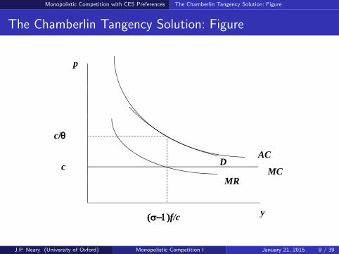
AC = AR ⇒ c + f /y = p+MC = MR ⇒ c + f /y = c/θ ⇒ y = (σ− 1) fc

Firm output depends only on σ, f , cIndustry output adjusts to demand shocks via changes in n onlyIn equilibrium: p = Ay−1/σ ⇒ A = py1/σ

i.e., Equilibrium A is also independent of P, I , and therefore n


Monopolistic Competition with CES Preferences The Chamberlin Tangency Solution: Figure

The Chamberlin Tangency Solution: Figure

p

c/

MRc MC

ACD

MR

1

f/c y


Monopolistic Competition with CES Preferences Technical Digression: Relative Curvature of AC and p

Technical Digression: Relative Curvature of AC and p

Proof that AC curve must be more convex than demand curve:

Unit-free measure of convexity of y = f (x): ρ ≡ − xf ′′f ′

Convexity of AC curve (or any rectangular hyperbola):

AC = c + fy → AC ′ = − f

y2 → AC ′′ = 2fy3 ⇒ ρAC = 2

Convexity of iso-elastic demand curve:

p = Ay−1σ → p′ = − 1

σAy− σ+1

σ = − 1σpy

→ p′′ = σ+1σ2 Ay−

2σ+1σ = σ+1

σpy2

⇒ ρp = σ+1σ ∈ (1, 2) provided σ ∈ (1, inf)

So: ρp < ρAC QED

This is consistent with:

Taste for diversity: Holds if and only if σ > 1Second-order condition for any functional form:

π = (p − AC )y → π′ = (p − AC ) + (p′ − AC ′)y→ π′′ = 2(p′ − AC ′) + (p′′ − AC ′′)y

⇒ π′′ < 0 IFF − yp′′

p′ < − yAC ′′

AC ′ ⇔ ρp < ρAC


Monopolistic Competition with CES Preferences The Role(s) of σ

The Role(s) of σ

High σ:

Different varieties are close substitutes for each other(preference for diversity is not so strong)p close to c : so p and MR curves are flat and close togethery large: economies of scale are highly exploitedFewer varieties, higher output of each

Low σ:

Different varieties are less close substitutes(greater preference for diversity)p >> c : so p and MR curves are steep and far aparty small: economies of scale are not highly exploitedMore varieties, lower output of each


Monopolistic Competition with CES Preferences The Role(s) of σ: Figure

The Role(s) of σ: Figure

p

B

A

MRMC

AC

MR(high )MR

(low )

1

yEffects of Changes in the Elasticity of Substitution


Monopolistic Competition with CES Preferences Equilibrium Anomalies

Equilibrium Anomalies

Strong properties of CES equilibrium:1 Price-cost margin depends only on σ: p

c = σσ−1

2 Output y depends only on c , f and σ: y = (σ− 1) fc3 All adjustment to other exogenous changes is via changes in n

How to avoid these implausible properties?1 Assume more than one factor with non-homothetic costs:

Lawrence-Spiller (1983), Flam-Helpman (1987), Forslid-Ottaviano(2003)

TC = rf + wcy ⇒ y = (σ− 1)r

w

f

c(5)

2 Assume heterogeneous firms: Melitz (2003)Infra-marginal firms make positive profits, so tangency condition doesnot hold

3 Relax CES assumption: Avoids all 3!Krugman (1979), Melitz-Ottaviano (2008), Zhelobodko-Kokovin-Parenti-Thisse (2011)


One-Sector Model with General Preferences

Plan of Lectures



3 One-Sector Model with General PreferencesAdditive SeparabilityThe Elasticity of DemandFirm and Industry EquilibriumFirm and Industry Equilibrium: FigureLabour-Market EquilibriumFirm, Industry and Labour-Market Equilibrium: FigureEffects of GlobalizationEffects of Globalization: FigureEffects of Globalization: Mark-UpsDigression: Sub- and SuperconvexityEffects of Globalization: Prices and OutputsEffects of Globalization: Firms and VarietiesEffects of Globalization: SummarySpecialising Additive Separability to CESGlobalization: The CES Special CaseGlobalization with Superconvex Demands



One-Sector Model with General Preferences Additive Separability

Additive Separability

Krugman JIE 1979: General additively separable preferences:

Probably the simplest possible fully-specified GE model in whichintra-industry trade could be rigorously demonstrated.

Suppose: k identical countries, n goods produced per country inequilibrium.

So: total number of varieties available in free trade is N = kn.

In each country there are L households, each of whom supplies a unitof labour (the only factor of production) and maximizes:

U =N

∑i=1

u (xi ) u′ (xi ) > 0, u′′ (xi ) < 0.

FOC gives inverse Frisch demand curves: u′ (xi ) = λpi . Appendix

Here λ is the individual household’s marginal utility of income, whichdepends on their income and on the prices of other goods.However, provided N is large, each firm rationally takes λ as fixed.Echoing Chamberlin, the demand curve a firm perceives for its ownproduct depends on its price only: pi = pi (xi ) ⇔ xi = xi (pi ).


One-Sector Model with General Preferences The Elasticity of Demand

The Elasticity of Demand

Total quantity demanded comes from all households in all countries,so market-clearing condition for the output of each firm is:

Goods-Market Equilibrium (GME): y = kLx (6)

With identical consumers, perceived elasticity of demand facing a firm,py

∂y∂p , depends only on consumption of an individual household x :

− pydydp = − p

kLx kLdxdp = − p

xdxdp .

Differentiating the demand function, this elasticity can be written as:

ε (x) ≡ − u′(x)xu′′(x) = −

p(x)xp′(x) = −

pxdxdp .

Krugman assumes ε(x) is decreasing in consumption: εx ≡ dε(x)dx < 0.

i.e., higher consumption, or, equivalently, a lower price, makeshouseholds less responsive to price.Equivalent to “sub-convexity”: demand function less convex than CES

Is this plausible? Does it matter?“Yes” and “Yes”: See below and “Not So Demanding”Mostly these notes assume this case; “*” denotes affected results


One-Sector Model with General Preferences Firm and Industry Equilibrium

Firm and Industry Equilibrium

Each firm maximizes profits by setting its marginal revenue given λequal to its marginal cost c .

c = aw in GE, but we set w = 1 by choice of numeraire.Writing FOC in terms of the perceived elasticity of demand ε (x), anddropping firm subscripts because of symmetry assumption, gives: App

Profit Maximization (MR=MC ):p

w=

ε (x)

ε (x)− 1c (7)

Recalling that ε (x) is decreasing in consumption, this implies thathigher levels of consumption allow firms to charge higher prices.Hence (7) is represented, for given values of k and L, by theupward-sloping locus MR=MC in the upper panel of Figure 1.

Second equilibrium condition in each sector: Profits are driven to zero:

Free Entry (p=AC ):p

w=

f

y+ c (8)

This implies a downward-sloping relationship between y and p/w .


One-Sector Model with General Preferences Firm and Industry Equilibrium: Figure

Firm and Industry Equilibrium: Figure

MR=MCp/w

A

p=AC

y

p=AC


One-Sector Model with General Preferences Labour-Market Equilibrium

Labour-Market Equilibrium

Each country’s labour supply L must equal the demand from alldomestic firms:

Labour-Market Equilibrium (LME ): L = n (f + cy) (9)

This equation implies a negative relationship between equilibrium firmsize y and the number of firms n, as illustrated in the lower panel ofFigure 1.

The full model then consists of the four equations (6), (7), (8), and(9), in four unknowns: p/w , x , y and n.


One-Sector Model with General Preferences Firm, Industry and Labour-Market Equilibrium: Figure

Firm, Industry and Labour-Market Equilibrium: Figure

MR=MCp/w

A

p=AC

y

p=AC

n

A'

LME

yJ.P. Neary (University of Oxford) Monopolistic Competition I January 21, 2015 20 / 39

One-Sector Model with General Preferences Effects of Globalization

Increase in the Number of Countries

Increase in k , representing the addition of more identical countries.

Equations (8) and (9), unaffected; only direct effect is to disruptgoods-market equilibrium (6).

World demand rises, so every firm must increase output by an equalamount if firms are to continue maximizing profits at the same prices.

Thus the MR=MC curve (7) shifts to the right.

If prices did not change, as at E , firms would now earn positiveprofits.

Hence, prices must fall and the new equilibrium must be at point B.


One-Sector Model with General Preferences Effects of Globalization: Figure

Effects of Globalization: Figure

MR=MCp/w

EA

B

p=AC

y

p=AC

n

A'

LME

B'

yJ.P. Neary (University of Oxford) Monopolistic Competition I January 21, 2015 22 / 39

One-Sector Model with General Preferences Effects of Globalization: Mark-Ups

Effects of Globalization: Mark-Ups

Firms move down their AC curves, producing more at lower costs,with benefits passed on to consumers in the form of lower prices.

Totally differentiating MR=MC (7) gives p = Eµx ; Eµ is the elasticityof the mark-up µ ≡ p

c with respect to consumption: Appendix

MR = MC : p =ε + 1− ερ

ε (ε− 1)x

Slope of MR=MC :px > 0 IFF ρ < ε+1

ε

i.e., IFF demand is “subconvex” Skip Subconvexity Sub-Section


One-Sector Model with General Preferences Digression: Sub- and Superconvexity

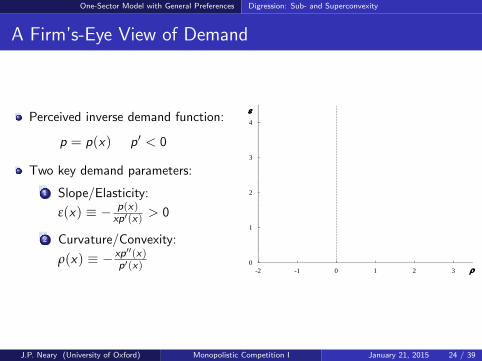
A Firm’s-Eye View of Demand

Perceived inverse demand function:

p = p(x) p′ < 0

Two key demand parameters:

1 Slope/Elasticity:

ε(x) ≡ − p(x)xp′(x) > 0

2 Curvature/Convexity:

ρ(x) ≡ − xp′′(x)p′(x)

4

4

3

2

11

0-2 -1 0 1 2 3



The Admissible Region

For a monopoly firm:

First-order condition:p+ xp′ = c ≥ 0 ⇒ ε ≥ 1

Second-order condition:2p′ + xp′′ < 0 ⇒ ρ < 2

4.0

4.0

3.0

2.0

1 01.0

0.0-2.0 -1.0 0.0 1.0 2.0 3.0



CES Demands

In general, both ε and ρ vary withsales

Exception: CES/iso-elastic case:

p = βx−1/σ

⇒ ε = σ, ρ = σ+1σ > 1

⇒ ε = 1ρ−1 0.0

1.0

2.0

3.0

4.0

-2.0 -1.0 0.0 1.0 2.0 3.0

CES

0.0

1.0

2.0

3.0

4.0

-2.0 -1.0 0.0 1.0 2.0 3.0

Cobb-Douglas

CES

Cobb-Douglas: ε = 1, ρ = 2; just on boundary of both FOC and SOC



Superconvexity

[Mrazova-Neary (2011)]

p(x) is superconvex at x0 IFF:

log p(x) is convex in log x

p(x) is more convex than a CESdemand function with the sameelasticity: ρ > ε+1

ε

ε is increasing in sales:

εx = εx

[ρ− ε+1

ε

]0.0

1.0

2.0

3.0

4.0

-2.0 -1.0 0.0 1.0 2.0 3.0

SC

Sub-Convex Super-Convex

A

C

B

0.0

1.0

2.0

3.0

4.0

-2.0 -1.0 0.0 1.0 2.0 3.0

SC


0.0

1.0

2.0

3.0

4.0

-2.0 -1.0 0.0 1.0 2.0 3.0

SC


“Globalization”[x ↓]

lowers mark-ups[ pc ↓]

IFF demands are subconvex

Because the mark-up is decreasing in elasticity: pc = ε

ε−1 = 1 + 1ε−1


One-Sector Model with General Preferences Effects of Globalization: Prices and Outputs

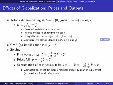
Effects of Globalization: Prices and Outputs

Totally differentiating AR=AC (8) gives p = −(1−ω)y .

ω ≡ cyf +cy = c

p

Share of variable in total costsInverse measure of returns to scaleIn equilibrium: ω = ε−1

ε ⇒ p = − 1ε y

Comparative statics depend only on ε and ρ Details

GME (6) implies that x = y − k.

Solving:

Firm output rises: y = ε+1−ερε(2−ρ)

k > 0∗

Prices fall: p = − 1ε y < 0∗

Consumption of each variety falls: x = y − k = − ε−1ε(2−ρ)

k < 0

Competition effect (in home market) offset by market-size effect(expansion of world demand).


One-Sector Model with General Preferences Effects of Globalization: Firms and Varieties

Effects of Globalization: Firms and Varieties

Because of the aggregate resource constraint, the lower panel of thefigure shows that an increase in firm output can only come about ifthe number of domestic firms falls.

The proportional change in the number of domestic firms (which is alsothe change in the number of domestically-produced varieties) is:

n = − ε−1ε y < 0∗.

However, the total number of varieties produced in the world rises, soconsumers benefit from an increase in diversity as well as a fall inprices.

The change in the total number of active firms in the world is:

N = k + n = (ε−1)2+(2−ρ)εε2(2−ρ)

k > 0.

Finally, because consumers demand all varieties, there is an increasein trade, all of which is intra-industry.

Share of trade in GNP = k−1k


One-Sector Model with General Preferences Effects of Globalization: Summary

Effects of Globalization with Subconvex Demands

k > 0:

y =ε + 1− ερ

ε (2− ρ)k > 0∗

p = −1

εy < 0∗

n = − ε− 1

εy < 0∗

x = y − k = − ε− 1

ε(2− ρ)k < 0

N = k+ n =(ε− 1)2 + (2− ρ) ε

ε2 (2− ρ)k > 0

* IFF demands are subconvex

CES Case Back

MR=MCp/w

EA

B

p=AC

y

p=AC

n

A'

LME

B'

y



Changes in Price and Number of Varieties

p = − ε + 1− ερ

ε2 (2− ρ)k

Negative IFF ρ < 1 + 1ε

Hetero

Always increasing in ρ

Increasing in ε IFF ρ < 1 + 2ε

N =(ε− 1)2 + (2− ρ) ε

ε2 (2− ρ)k

Always positive BP Pollak

Always increasing in ρ NPOLLAK

Decreasing in ε IFF ρ < 2ε



Summary

Krugman’s landmark 1979 paper was thus the first to present a coherentgeneral-equilibrium analysis of the kind of trade that, in the words of theNobel Memorial Prize Committee: “enables specialization and large-scaleproduction, which results in lower prices and a greater diversity ofcommodities.” It was arguably also the last, since most of the subsequentliterature has concentrated on a special case in which only the finalprediction, a greater diversity of goods consumed, remains true. Theproblem which soon emerged is that, though the model is deceptivelysimple, for most purposes it is not nearly simple enough. In particular, thegeneral [additively separable] Dixit-Stiglitz specification does not yieldclosed-form solutions. As a result, Krugman himself . . . and mostsubsequent writers on monopolistic competition and trade have workedwith . . .

Neary (2009)


One-Sector Model with General Preferences Specialising Additive Separability to CES

Specialising Additive Separability to CES

CES: Uθ =n

∑i=1

x θi , 0 < θ = σ−1

σ < 1, θ fixed.

MR = MC locus (7) is horizontal, and is unaffected by changes in k.⇒ Profit maximization fixes price-cost margin: p

c = σσ−1 .

Free entry fixes the size of each firm as a function only of σ and theratio of fixed to variable costs: from (7) and (8), y = (σ− 1) f

c .Increase in k : initial equilibrium in Figure 1 is unaffected [Eµ = 0]:

No change at all in price-cost margins, scale of production, or n.Only the destination of home output changes, with a larger shareexported in exchange for more imports, leading to a greater range ofvarieties, and thus higher utility, for domestic consumers.The fact that even n does not change is an artefact of the particularshock (rise in k); e.g., a rise in population of each country, L, shiftsLME upwards, so inducing entry of more firms.Still: most shocks leave firm scale unaffected, with adjustment indomestic production coming via changes in the number of firms.

CES case de-emphasizes increasing returns; concentrates attention onthe range of varieties available to consumers.


One-Sector Model with General Preferences Globalization: The CES Special Case

Globalization: The CES Special Case

k > 0, ε = σ:

p = 0

y = 0

n = 0

x = y − k = −k < 0

N = k + n = k > 0

Back to Subconvex Case

p/w

AMR=MC

p=AC

y

p=AC

n

A'

LME

y


One-Sector Model with General Preferences Globalization with Superconvex Demands

Globalization with Superconvex Demands

MR=MC now slopes downwards

Multiple equilibria are possible

C is unstable

Globalization shifts MR=MC up

Equilibrium moves from A → B

Comparative statics reversed forp, y , n

y

n

LME

MR=MC

p/w

y

EA

B

p=AC

A'

B'

C


Supplementary Notes

Plan of Lectures




4 Supplementary NotesComparison with Krugman 1979Frisch DemandsDerivations of Comparative Statics


Supplementary Notes Comparison with Krugman 1979

Comparison with Krugman 1979

Notation etc. is similar to Krugman’s with some differences:

1 Krugman uses a different notation for the utility function:

u =N

∑i=1

v (xi ) v ′ (xi ) > 0, v ′′ (xi ) < 0

2 Krugman assumes subconvexity: “it seems to be necessary if themodel is to yield reasonable results, and I make the assumptionwithout apology.”

3 Krugman draws the MR=MC and p=AC curves in {p/w , x} spacerather than {p/w , y} space as I do. This is slightly more natural, butmisses out on the link with the LME locus.


Supplementary Notes Frisch Demands

Frisch Demands

Different kinds of demand functions:

Direct Inverse

Marshallian x(p, I ) p(x , I )Hicksian x(p, u) p(x , u)Frisch x(p, λ) p(x , λ)

Each of these depends in general on a vector of prices or outputs

Special feature of additively separable preferences:

Given λ, Frisch demands depend only on own price/output

Back to text


Supplementary Notes Derivations of Comparative Statics

Derivations of Comparative Statics

Derivation of Marginal Revenue with General Demands:

TR = xp(x) ⇒ MR = xp′ + p =(

1 + xp′

p

)p =

(1− 1

ε

)p = ε−1

ε p

Back to text

Total Derivative of (7):

p = µc ⇒ p = µ = Eµx ; Eµ ≡ − 1ε(x)−1

xε(x)

dε(x)dx > 0

Express Eµ in terms of ε and ρ:

ε(x) ≡ − p(x)xp′(x) ⇒ εx = − 1

(xp′)2

[x(p′)2 − p(p′ + xp′′)

]= − p

x2p′

[xp′

p − 1− xp′′

p′

]= ε

x

(ρ− 1− 1

ε

)⇒ Eµ = 1

ε−1

(ε+1

ε − ρ)

Back to text


monopolistic competition in trade i - university of...

Documents