monocular rivalry exhibits three hallmarks of binocular

This article may not exactly replicate the final version published. It is not the copy of record. 1

Monocular rivalry exhibits three hallmarks of binocular

rivalry

Robert P. O’Shea1*, David Alais2, Amanda L. Parker2

and David J. La Rooy1

1Department of Psychology, University of Otago, PO Box 56,

Dunedin, New Zealand

2 School of Psychology, The University of Sydney, Australia

* Corresponding author: e-mail: [email protected]

Acknowledgements: We are grateful to Frank Tong for allowing us to use his stimuli for

Experiment 2, and to Janine Mendola for helpful discussion.

O'Shea, R. P., Parker, A. L., La Rooy, D. J. & Alais, D. (2009).Monocular rivalry exhibits

three hallmarks of binocular rivalry: Evidence for common processes. Vision

Research, 49, 671–681. http://www.elsevier.com/wps/find/journaldescription.cws_home/263/descri

ption#description


Abstract

Binocular rivalry occurs when different images are presented one to each eye: the images

are visible only alternately. Monocular rivalry occurs when different images are

presented both to the same eye: the clarity of the images fluctuates alternately. Could

both sorts of rivalry reflect the operation of a general visual mechanism for dealing with

perceptual ambiguity? We report four experiments showing similarities between the two

phenomena. First, we show that monocular rivalry can occur with complex images, as

with binocular rivalry, and that the two phenomena are affected similarly by the size and

colour of the images. Second, we show that the distribution of dominance periods during

monocular rivalry has a gamma shape and is stochastic. Third, we show that during

periods of monocular-rivalry suppression, the threshold to detect a probe (a contrast pulse

to the suppressed stimulus) is raised compared with during periods of dominance. The

threshold elevation is much weaker than during binocular rivalry, consistent with

monocular rivalry’s weak appearance. We discuss other similarities between monocular

and binocular rivalry, and also some differences, concluding that part of the processing

underlying both phenomena is a general visual mechanism for dealing with perceptual

ambiguity.


Monocular rivalry exhibits three hallmarks of binocular

rivalry: Evidence for common processes

We experience the visual world in astounding richness and detail, yet our

knowledge of how these conscious percepts arise is still quite poor (cf. Chalmers, 1995).

One way to learn more about these processes is to study phenomena in which visual

consciousness changes without any change in the stimuli being viewed (Crick & Koch,

1995). Such phenomena are known as perceptually multistable and include binocular

rivalry (Porta, 1593, cited in Wade, 1996), reversals of the Necker cube (Necker, 1832),

of the Rubin face-vase figure (Rubin, 1915), and of the kinetic depth effect (Wallach &

O'Connell, 1953), and motion-induced blindness (Bonneh, Cooperman, & Sagi, 2001).

Binocular rivalry is a particularly fascinating example, in which visual consciousness

fluctuates randomly between two different images presented one to each eye. It has been

studied extensively (for reviews see Alais & Blake, 2005; Blake & O’Shea, In press) and

has gone some way to shedding light on how visual awareness arises: Conscious visual

experience in binocular rivalry is thought to arise from activation, and suppression, of

neurons at a succession of stages in the visual system (e.g., Blake & Logothetis, 2002).

Our interest in this paper is in the relationship between binocular rivalry and

another phenomenon of perceptual multistability, monocular rivalry. Monocular rivalry

was discovered by Breese (1899) in the course of his foundational observations and

experiments on binocular rivalry. He found that binocular-rivalry-like behaviour also

occurred when a red and a green grating were optically superimposed by a prism and

presented to a single eye. Breese called it monocular rivalry to distinguish it from

binocular rivalry. He reported that monocular rivalry alternations tended to occur at a

slower rate than binocular rivalry alternations and that the perceptual alternations were

less vivid: “Neither disappeared completely: but at times the red would appear very

distinctly while the green would fade; then the red would fade and the green appear

distinctly” (p. 43).

One of the unresolved questions in the literature on perceptual multistability is

whether common neural mechanisms underlie binocular and monocular rivalry. There are

at least three general similarities between the two forms of rivalry that suggest


commonality. First, the basic phenomenology is similar in that both involve periods of

alternating dominance. Second, both forms of rivalry become more vigorous as stimuli

are made more different in colour (e.g., Wade, 1975), or in orientation and spatial

frequency (e.g.,Atkinson, Fiorentini, Campbell, & Maffei, 1973; Campbell, Gilinsky,

Howell, Riggs, & Atkinson, 1973; O’Shea, 1998). Third, the two forms of rivalry can

influence each other, tending to synchronize their alternations in adjacent regions of the

visual field (Andrews & Purves, 1997; Pearson & Clifford, 2005).

Although monocular and binocular rivalry are similar in these three respects, this

is by no means an exhaustive list of possible comparisons between the two rivalries. Here

we test whether monocular rivalry shares three other hallmarks of binocular rivalry. First,

binocular rivalry can occur between any two images, providing they are sufficiently

different. For example, Porta (1593, cited in Wade, 1996) observed rivalry between two

different pages of text. Wheatstone (1838) observed rivalry between two alphabetic

letters. Galton (1907) observed rivalry between pictures of different faces. Yet, with the

possible exception of a study by Boutet and Chaudhuri (2001), monocular rivalry has

always been shown between simple repetitive stimuli such as gratings, leading some to

suppose that such stimuli are necessary for monocular rivalry (e.g., Furchner & Ginsburg,

1978; Georgeson, 1984; Georgeson & Phillips, 1980; Maier, Logothetis, & Leopold,

2005). In Experiments 1 and 2, we show that monocular rivalry occurs between complex

pictures of faces and houses.

Second, binocular rivalry has a characteristic distribution of dominance times, a

gamma distribution, and the duration of one episode of dominance cannot be predicted by

any of the preceding ones (e.g., Fox & Herrmann, 1967; Levelt, 1967). Yet the

distribution and predictability of episodes of monocular rivalry dominance are unknown.

In Experiment 3, we show that the temporal periods of monocular rivalry are similar to

those of binocular rivalry: gamma distributed and independent.

Third binocular rivalry suppression is accompanied by a characteristic loss of

visual sensitivity. When a stimulus is suppressed during binocular rivalry and becomes

invisible, stimuli presented to the same retinal region are also invisible, provided the new

stimuli are not so abrupt or so bright as to break suppression (indicative of suppression of

the whole eye) (e.g., Fox & McIntyre, 1967; Nguyen, Freeman, & Alais, 2003; Norman,


Norman, & Bilotta, 1999; Wales & Fox, 1970). This is usually demonstrated by showing

a loss of sensitivity during periods of suppression relative to periods of dominance,

however it is unknown whether monocular rivalry also shows such suppression effects. In

Experiment 4, we show that monocular rivalry does indeed produce threshold elevations

during suppression, although the effect is weaker than in binocular rivalry.

The experiments in this paper have been published in abstract form (O’Shea,

Alais, & Parker, 2005; O’Shea, Alais, & Parker, 2006; O’Shea & La Rooy, 2004).

Experiment 1

Maier et al. (2005) reviewed studies of monocular rivalry, and concluded that monocular

rivalry occurs only between simple, faint, repetitive images, such as low-contrast

gratings. They observed, however, that alternations in clarity could occur between

complex images, such as the surface of a pond and a reflection on it of a tree, although

they did not measure rivalry with such stimuli. Boutet and Chaudhuri (2001) optically

superimposed two faces that differed in orientation by 90 deg. They reported that the two

faces alternated in clarity in a rivalry-like way, but they did not measure rivalry

conventionally. They forced observer’s choices about whether one or two faces was seen

after brief stimulus presentations of 1 to 3 s. Monocular rivalry, however, usually takes

several seconds, or even tens of seconds, before oscillations become evident (e.g., Breese,

1899). We decided to measure monocular rivalry with complex images in a conventional

way, by showing observers optically superimposed images for one-minute trials, and

asking them to track their perceptual alternations using key presses. We used images of

faces and houses. Moreover, we explicitly compared monocular rivalry with binocular

rivalry for identical stimuli over a range of stimulus sizes.

Method

Observers

Three males and one female volunteered for this experiment after giving informed

consent. All had normal or corrected-to-normal vision. DLR (age 33), HF (age 23), and

RS (age 24) had some experience as observers; ROS (age 50) was a highly trained

observer. All observers were right handed. HF and RS were naive as to the purpose of the

experiment.


Stimuli and Apparatus

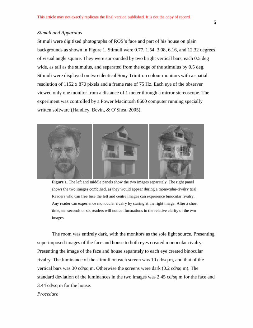
Stimuli were digitized photographs of ROS’s face and part of his house on plain

backgrounds as shown in Figure 1. Stimuli were 0.77, 1.54, 3.08, 6.16, and 12.32 degrees

of visual angle square. They were surrounded by two bright vertical bars, each 0.5 deg

wide, as tall as the stimulus, and separated from the edge of the stimulus by 0.5 deg.

Stimuli were displayed on two identical Sony Trinitron colour monitors with a spatial

resolution of 1152 x 870 pixels and a frame rate of 75 Hz. Each eye of the observer

viewed only one monitor from a distance of 1 meter through a mirror stereoscope. The

experiment was controlled by a Power Macintosh 8600 computer running specially

written software (Handley, Bevin, & O’Shea, 2005).

Figure 1. The left and middle panels show the two images separately. The right panel

shows the two images combined, as they would appear during a monocular-rivalry trial.

Readers who can free fuse the left and centre images can experience binocular rivalry.

Any reader can experience monocular rivalry by staring at the right image. After a short

time, ten seconds or so, readers will notice fluctuations in the relative clarity of the two

images.

The room was entirely dark, with the monitors as the sole light source. Presenting

superimposed images of the face and house to both eyes created monocular rivalry.

Presenting the image of the face and house separately to each eye created binocular

rivalry. The luminance of the stimuli on each screen was 10 cd/sq m, and that of the

vertical bars was 30 cd/sq m. Otherwise the screens were dark (0.2 cd/sq m). The

standard deviation of the luminances in the two images was 2.45 cd/sq m for the face and

3.44 cd/sq m for the house.

Procedure


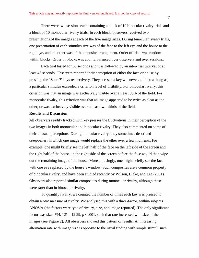
There were two sessions each containing a block of 10 binocular rivalry trials and

a block of 10 monocular rivalry trials. In each block, observers received two

presentations of the images at each of the five image sizes. During binocular rivalry trials,

one presentation of each stimulus size was of the face to the left eye and the house to the

right eye, and the other was of the opposite arrangement. Order of trials was random

within blocks. Order of blocks was counterbalanced over observers and over sessions.

Each trial lasted for 60 seconds and was followed by an inter-trial interval of at

least 45 seconds. Observers reported their perception of either the face or house by

pressing the ‘Z' or '?' keys respectively. They pressed a key whenever, and for as long as,

a particular stimulus exceeded a criterion level of visibility. For binocular rivalry, this

criterion was that an image was exclusively visible over at least 95% of the field. For

monocular rivalry, this criterion was that an image appeared to be twice as clear as the

other, or was exclusively visible over at least two-thirds of the field.

Results and Discussion

All observers readily tracked with key presses the fluctuations in their perception of the

two images in both monocular and binocular rivalry. They also commented on some of

their unusual perceptions. During binocular rivalry, they sometimes described

composites, in which one image would replace the other over a few moments. For

example, one might briefly see the left half of the face on the left side of the screen and

the right half of the house on the right side of the screen before the face would then wipe

out the remaining image of the house. More amusingly, one might briefly see the face

with one eye replaced by the house’s window. Such composites are a common property

of binocular rivalry, and have been studied recently by Wilson, Blake, and Lee (2001).

Observers also reported similar composites during monocular rivalry, although these

were rarer than in binocular rivalry.

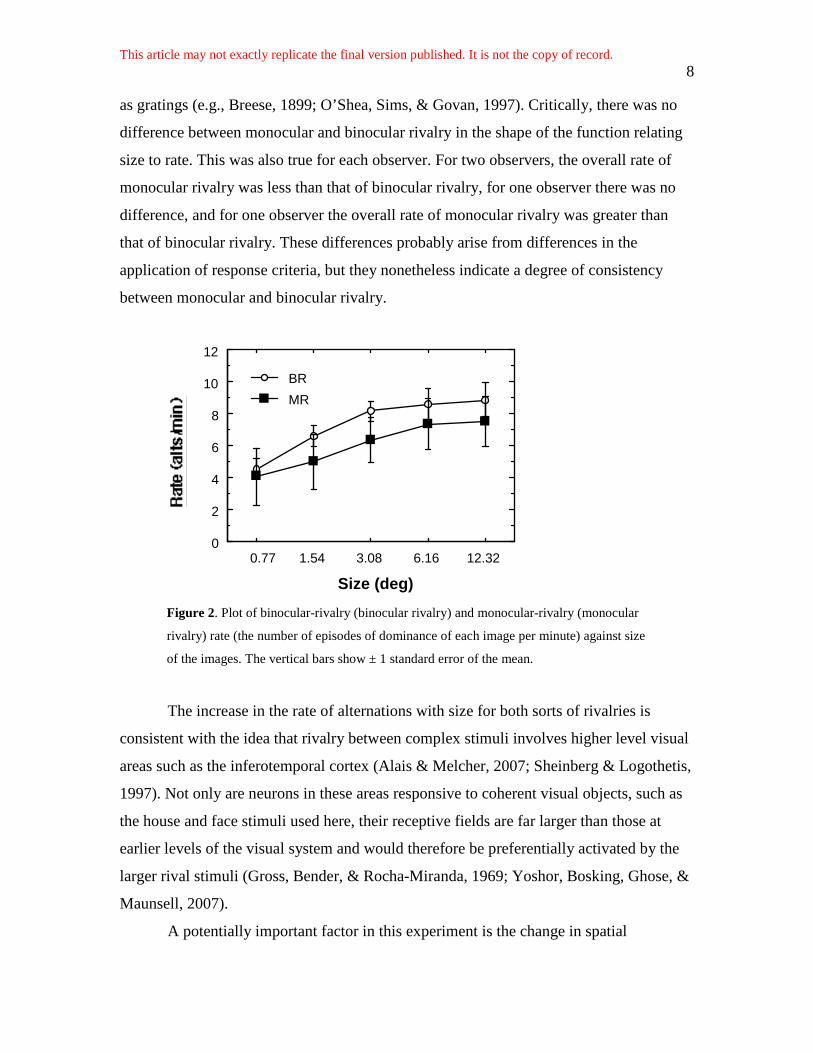
To quantify rivalry, we counted the number of times each key was pressed to

obtain a rate measure of rivalry. We analysed this with a three-factor, within-subjects

ANOVA (the factors were type of rivalry, size, and image reported). The only significant

factor was size, F(4, 12) = 12.29, p < .001, such that rate increased with size of the

images (see Figure 2). All observers showed this pattern of results. An increasing

alternation rate with image size is opposite to the usual finding with simple stimuli such


as gratings (e.g., Breese, 1899; O’Shea, Sims, & Govan, 1997). Critically, there was no

difference between monocular and binocular rivalry in the shape of the function relating

size to rate. This was also true for each observer. For two observers, the overall rate of

monocular rivalry was less than that of binocular rivalry, for one observer there was no

difference, and for one observer the overall rate of monocular rivalry was greater than

that of binocular rivalry. These differences probably arise from differences in the

application of response criteria, but they nonetheless indicate a degree of consistency

between monocular and binocular rivalry.

0

2

4

6

8

10

12

0.77 1.54 3.08 6.16 12.32

Size (deg)

MR

BR

Figure 2. Plot of binocular-rivalry (binocular rivalry) and monocular-rivalry (monocular

rivalry) rate (the number of episodes of dominance of each image per minute) against size

of the images. The vertical bars show ± 1 standard error of the mean.

The increase in the rate of alternations with size for both sorts of rivalries is

consistent with the idea that rivalry between complex stimuli involves higher level visual

areas such as the inferotemporal cortex (Alais & Melcher, 2007; Sheinberg & Logothetis,

1997). Not only are neurons in these areas responsive to coherent visual objects, such as

the house and face stimuli used here, their receptive fields are far larger than those at

earlier levels of the visual system and would therefore be preferentially activated by the

larger rival stimuli (Gross, Bender, & Rocha-Miranda, 1969; Yoshor, Bosking, Ghose, &

Maunsell, 2007).

A potentially important factor in this experiment is the change in spatial


frequency content that occurs when images are scaled up or down in size. In the case of

pictures, increasing the image size lengthens the period of the spatial modulations,

lowering the spatial frequency content of the images in direct proportion to the scale

factor. This can be contrasted with grating stimuli, where a change in size would

normally be achieved by keeping the spatial frequency constant and simply showing

more cycles in the image. The image sizes used in Experiment 1 varied over a four-

octave range. Since it has been shown that monocular rivalry is usually strongest at low

spatial frequencies (Kitterle & Thomas, 1980; Mapperson & Lovegrove, 1984; O’Shea,

1998), the effect of increasing alternation rate with larger images shown in Figure 2

might be related to the lowering of spatial frequency. However, all these studies used

grating stimuli, which contain a single spatial frequency, whereas our images are

complex with a very broad spatial frequency spectrum. Increasing the size of broadband

images extends the spatial spectrum at the lower end, but they remain broadband over a

very large spatial range and this makes comparison with grating studies difficult.

Of more central importance for our purposes is that both monocular rivalry and

binocular rivalry (which is robust over a very large range of spatial frequencies (O’Shea

et al., 1997) exhibited the same trend of increasing alternation rate with increasing image

size. Given this, the similar trends shown in Figure 2 may be indicative of common

mechanisms in monocular and binocular rivalry. We further test this idea in the next

experiment by assessing the effects on the two sorts of rivalries of adding colour

differences to the two rivalling images.

Experiment 2

Monocular rivalry does not require coloured stimuli (e.g., Experiment 1), but its

alternation rate is faster when stimuli have complementary colours (Campbell & Howell,

1972; Rauschecker, Campbell, & Atkinson, 1973; Wade, 1975). Similarly, binocular

rivalry does not require coloured stimuli, but its alternation rate is also faster when the

rival stimuli have complementary colours (Hollins & Leung, 1978; Thomas, 1978; Wade,

1975). The only study we are aware of in which the effects of colour on monocular and

binocular rivalry were compared in the same experiment with the same observers used

grating stimuli and found that colour affected monocular but not binocular rivalry

(Kitterle & Thomas, 1980). In Experiment 2, we also examine the role of colour on


binocular and monocular rivalry but extend it to include complex broadband images.

Method

The Method of Experiment 2 was very similar to that of Experiment 1. The differences

were that a second set of stimuli, that used by Tong, Nakayama, Vaughan, and Kanwisher

(1998) was used, and one of the male observers from Experiment 1 did not participate.

All stimuli were 6.16 deg square; Pixel luminances in Tong et al.’s face and house had

standard deviations of 3.22 cd/sq m and 4.98 cd/sq m respectively. There were 12

binocular-rivalry and 12 monocular-rivalry trials in which observers again tracked their

rivalry alternations. In four repetitions of each pair of stimuli the images were

achromatic, in four the face was red (CIE x = .315, y = .321) and the house green (CIE x

= .270, y = .347), and in four the face was green and the house red.


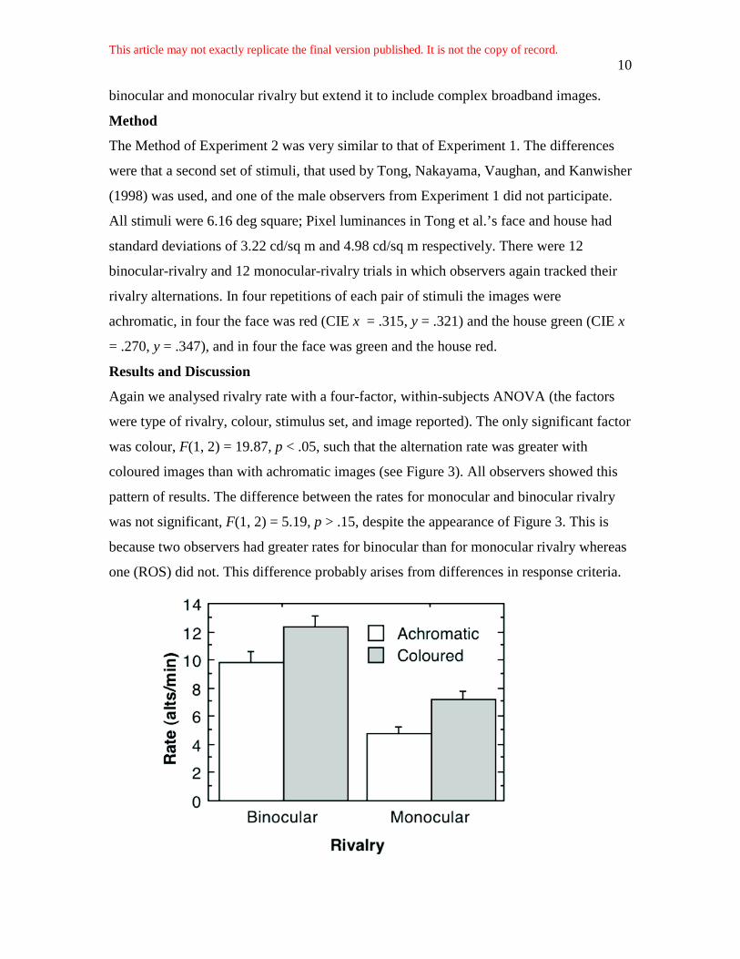
Again we analysed rivalry rate with a four-factor, within-subjects ANOVA (the factors

were type of rivalry, colour, stimulus set, and image reported). The only significant factor

was colour, F(1, 2) = 19.87, p < .05, such that the alternation rate was greater with

coloured images than with achromatic images (see Figure 3). All observers showed this

pattern of results. The difference between the rates for monocular and binocular rivalry

was not significant, F(1, 2) = 5.19, p > .15, despite the appearance of Figure 3. This is

because two observers had greater rates for binocular than for monocular rivalry whereas

one (ROS) did not. This difference probably arises from differences in response criteria.


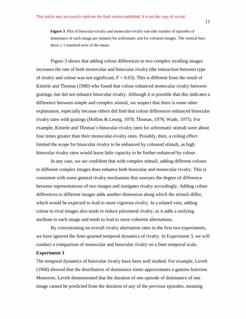
Figure 3. Plot of binocular-rivalry and monocular-rivalry rate (the number of episodes of

dominance of each image per minute) for achromatic and for coloured images. The vertical bars

show ± 1 standard error of the mean.

Figure 3 shows that adding colour differences to two complex rivalling images

increases the rate of both monocular and binocular rivalry (the interaction between type

of rivalry and colour was not significant, F = 0.03). This is different from the result of

Kitterle and Thomas (1980) who found that colour enhanced monocular rivalry between

gratings, but did not enhance binocular rivalry. Although it is possible that this indicates a

difference between simple and complex stimuli, we suspect that there is some other

explanation, especially because others did find that colour differences enhanced binocular

rivalry rates with gratings (Hollins & Leung, 1978; Thomas, 1978; Wade, 1975). For

example, Kitterle and Thomas’s binocular-rivalry rates for achromatic stimuli were about

four times greater than their monocular-rivalry rates. Possibly, then, a ceiling effect

limited the scope for binocular rivalry to be enhanced by coloured stimuli, as high

binocular rivalry rates would leave little capacity to be further enhanced by colour.

In any case, we are confident that with complex stimuli, adding different colours

to different complex images does enhance both binocular and monocular rivalry. This is

consistent with some general rivalry mechanism that assesses the degree of difference

between representations of two images and instigates rivalry accordingly. Adding colour

differences to different images adds another dimension along which the stimuli differ,

which would be expected to lead to more vigorous rivalry. In a related vein, adding

colour to rival images also tends to reduce piecemeal rivalry, as it adds a unifying

attribute to each image and tends to lead to more coherent alternations.

By concentrating on overall rivalry alternation rates in the first two experiments,

we have ignored the finer-grained temporal dynamics of rivalry. In Experiment 3, we will

conduct a comparison of monocular and binocular rivalry on a finer temporal scale.

Experiment 3

The temporal dynamics of binocular rivalry have been well studied. For example, Levelt

(1968) showed that the distribution of dominance times approximates a gamma function.

Moreover, Levelt demonstrated that the duration of one episode of dominance of one

image cannot be predicted from the duration of any of the previous episodes, meaning


that each dominance episode is a statistically independent sample from an underlying

population distribution of dominance times. We set out to determine whether monocular

rivalry also conforms to these principles, comparing it with binocular rivalry dynamics

measured on identical binocular-rivalry stimuli.

Method

Observers

Two of the authors acted as observers, ROS and AP. AP was 25.99 years old. Both

observers have normal vision.

Apparatus

The computer controlling this experiment was a Macintosh G4, running MatLab 5.2

scripts that used the Psychophysics Toolbox (Brainard, 1997; Pelli, 1997). Stimuli were

displayed on a 19-inch XYZ monitor showing 1024 x 768 pixels at a 75 Hz vertical

refresh rate. Stimuli were shown one on each side of the screen and viewed via a mirror

stereoscope at a viewing distance of 1999 cm.

Visual Stimuli

Stimuli were two orthogonal square-wave gratings, one red (CIE???) and the other green

(CIE???), oriented ±45° to vertical. The gratings had a spatial frequency of 2.2 cycles/deg

with a Michelson contrast of 8% and were placed in a circular aperture subtending 4.6°.

Gratings had a mean luminance of 19.99 cd/sq m; the background had a luminance of

19.99 cd/sq m. The gratings were superimposed and visible to both eyes for monocular

rivalry conditions; the gratings were presented one to each eye for binocular rivalry

conditions.

Procedure

For both binocular and monocular rivalry, the observer’s task was similar to that in

Experiment 1: to track episodes of perceptual dominance of one and the other stimuli by

pressing keys on the computer keyboard. There were x trials lasting 5 minutes for each

viewing condition. Viewing condition was alternated for each observer over trials; each

observer started with a different condition [if true!].


We analysed the records of rivalry in two ways. First, we plotted distributions of

dominance times to which we fitted Gamma functions. Specifically, we divided each


dominance duration by the mean for that observer and that condition, we constructed the

distribution, and we fit Gamma functions using a weighted least-squares algorithm.

Second, we computed autocorrelations between the recorded dominance sequence and

the same sequence offset by various time lags in order to test the sequential independence

of rivalry dominance times.

Figure 4 shows the distributions of dominance times separately for monocular and

binocular rivalry for each observer. All four plots exhibit the classic Gamma distribution

shape, rather like a positively skewed normal distribution; the smooth curves show the

best fitting Gamma distribution function. The parameters of all four fits are remarkably

similar, showing that monocular and binocular rivalry exhibit globally similar alternation

dynamics. This is especially true for ROS, although for AP there was an over-

representation of long dominance durations in monocular rivalry relative to binocular

rivalry that is not well captured by the best-fitting Gamma distribution.

Figure 4. Distribution of dominance times for two observers for binocular rivalry (top row) and

for monocular rivalry (bottom row). The continuous plot shows that best-fitting Gamma

distribution fitted to the data. The dominance durations were binned into 150 ms intervals and

were normalised to the mean duration.

Figure 5 shows the autocorrelation analyses for binocular and monocular rivalry.

The correlation is arbitrarily 1.0 when there is no lag. Similar to binocular rivalry (Levelt,

1968), that there no tendency for a given dominance duration to be related to the previous

dominance duration, or to dominance durations several phases earlier.. Overall, for all of

the four autocorrelation analyses, none of the correlations at any phase lag (from 1 to 12)

were statistically significant.

Figure 5. Results of the autocorrelation analysis for two observers for binocular rivalry (top row)

and for monocular rivalry (bottom row). Apart from the arbitrarily perfect autocorrelation when

the signal was not lagged, there were no statistically significant deviations from zero. 95%

confidence intervals around the correlation at each non-zero lag included a correlation of zero.


Experiment 4

One technique commonly used to study binocular rivalry has been to measure the depth

of suppression. This is done by measuring the detection threshold for a probe stimulus

presented to an eye during suppression, and comparing it against the threshold for the

same probe measured during dominance (Blake & Camisa, 1979; Blake & Fox, 1974;

Fox & Check, 1972; Wales & Fox, 1970). Generally, for simple stimuli such as gratings

and contours, probe sensitivity is reduced during suppression to about 60% of the level

measured during dominance (Fox & McIntyre, 1967; Nguyen et al., 2003; Norman et al.,

1999; Wales & Fox, 1970), although for higher-level stimuli such as faces and complex

global motions and forms, sensitivity is reduced to about 30% of the dominance level

(Alais & Melcher, 2007; Alais & Parker, 2006).

Surprisingly, the probe technique has never been used to assess the depth of

monocular rivalry suppression. We set out to do so. Of course, it is not possible to use

monocular probes (as done in binocular rivalry probe experiments) for monocular rivalry

because the rivalling stimuli are both present in the same eye. Instead, our approach was

to use a contrast increment of one of the monocular rivalry stimuli as a probe. We used

red and green orthogonal gratings oriented ±45° to vertical and we briefly and smoothly

pulsed the luminance of the red grating according to a temporal Gaussian profile, varying

the amplitude of the pulse to find the threshold. These thresholds were measured during

dominance and suppression to quantify suppression depth for monocular rivalry. As a

comparison, we also measured suppression depth for the same stimuli under binocular

rivalry conditions.

Method

The Method was similar to that of Experiment 3 with the following exceptions. Two new

observers volunteered for the experiment for a total of four, one of us (DA), an

experienced observer aged 29.99, and JT, an inexperienced observer naive to the

purposes of the experiment aged 19.99. All observers had normal vision. Instead of

tracking monocular or binocular rivalry observers pressed a key either whenever the red

or the green grating was dominant. Randomly on 50% of trials this caused a probe, a

contrast increment, to appear briefly on the red grating. Observers then made another

keypress to say whether the probe appeared or not. Feedback was given for correct and


incorrect responses. The probe followed the first keypress by 1999 ms, and had a

Gaussian profile over time (with a half-width of 67 ms) to ensure the probe was smooth

and free of transients. The Gaussian amplitude had a variable peak that was controlled by

an adaptive QUEST procedure (Watson & Pelli, 1983) involving two randomly

interleaved staircases to find the contrast increment threshold for the probe. Each QUEST

was preceded by four practice trials and comprised 40 trials. Observers responded to at

least four QUESTs in each of four conditions (probe presented during dominance vs

suppression and monocular vs binocular rivalry). Observers alternated between

dominance and suppression conditions, and alternated between monocular and binocular

rivalry. Starting condition was counterbalanced over sessions and over observers.


We analysed the mean thresholds for the four observers using a two-way, within-subjects

ANOVA. This found both main effects (rivalry type: monocular vs. binocular; and rivalry

phase: dominance vs. suppression) to be significant, but critically there was an interaction

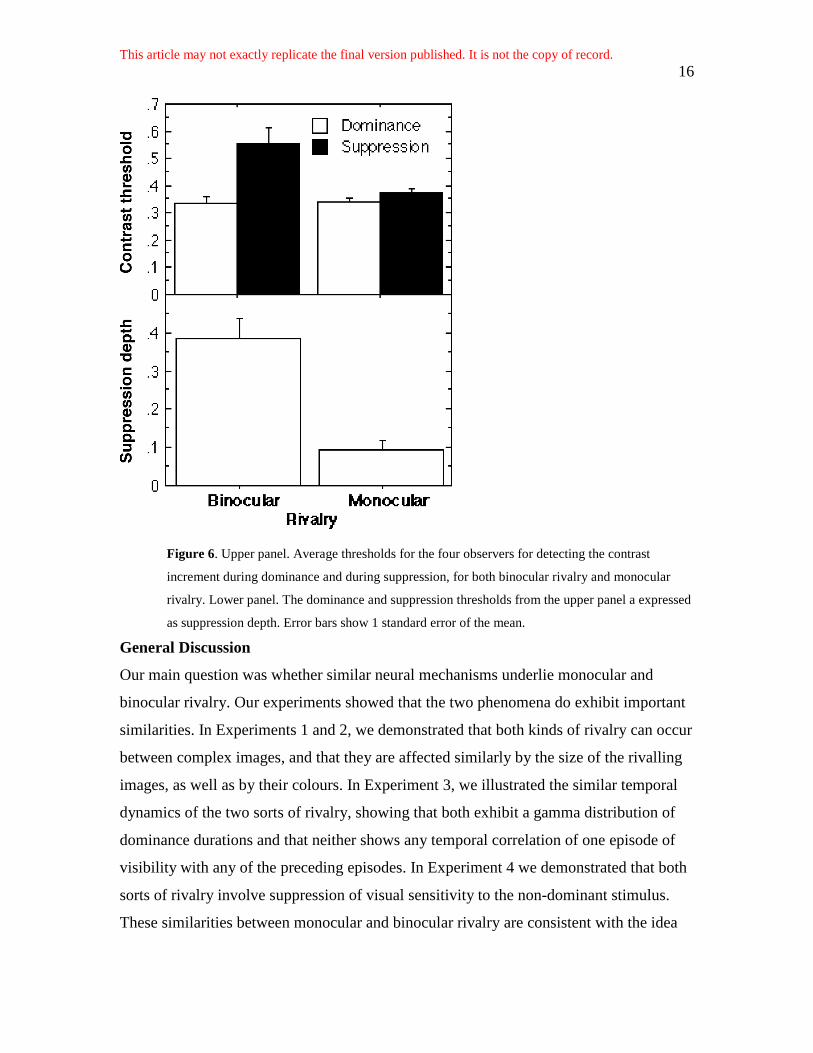
between them, F(1, 3) = 21.12, p < .05. The thresholds are shown in the upper panel of

Figure 6. Suppression depths are shown in the lower panel of Figure 6. Suppression depth

is calculated by subtracting from unity the ratio of the dominance threshold to the

suppression threshold. A suppression depth of zero, complete absence of suppression,

would occur if suppression and dominance thresholds were equal. Suppression depths

approach unity, complete suppression, when suppression thresholds are much greater

than dominance thresholds. For binocular rivalry, typical suppression depths are around

0.40 (e.g., Fox & McIntyre, 1967; Nguyen et al., 2003; Norman et al., 1999; Wales &

Fox, 1970); the lower panel of Figure 6 shows that the suppression depth we measured

for binocular rivalry is consistent with this value. By contrast, suppression depth for

monocular rivalry is much weaker at around 0.10. Although this value is significantly

greater than zero, t(3) = 4.67, p < .05, it is several times shallower than suppression depth

for binocular rivalry.


Figure 6. Upper panel. Average thresholds for the four observers for detecting the contrast

increment during dominance and during suppression, for both binocular rivalry and monocular

rivalry. Lower panel. The dominance and suppression thresholds from the upper panel a expressed

as suppression depth. Error bars show 1 standard error of the mean.

General Discussion

Our main question was whether similar neural mechanisms underlie monocular and

binocular rivalry. Our experiments showed that the two phenomena do exhibit important

similarities. In Experiments 1 and 2, we demonstrated that both kinds of rivalry can occur

between complex images, and that they are affected similarly by the size of the rivalling

images, as well as by their colours. In Experiment 3, we illustrated the similar temporal

dynamics of the two sorts of rivalry, showing that both exhibit a gamma distribution of

dominance durations and that neither shows any temporal correlation of one episode of

visibility with any of the preceding episodes. In Experiment 4 we demonstrated that both

sorts of rivalry involve suppression of visual sensitivity to the non-dominant stimulus.

These similarities between monocular and binocular rivalry are consistent with the idea


that the their underlying processes involve common neural mechanisms (cf. Leopold &

Logothetis, 1999; O’Shea, 1998; Papathomas, Kovács, Fehér, & Julesz, 1999).

Although the conclusion that monocular and binocular rivalry share common

processes has appeal, there are alternative explanations that need to be considered and

certain notable differences between the two phenomena must be addressed. One of the

competing explanations of monocular rivalry is that it is not strictly a perceptual

alternation but an epiphenomenon produced by a combination of eye movements and

afterimages. This line of argument has been proposed by Furchner and Ginsburg (1978),

by Georgeson and Phillips (1980), and by Georgeson (1984). They maintained that in the

case of two superimposed orthogonal gratings, for example, steady fixation will build up

afterimages that would tend to cancel visibility of both. If an eye movement were made in

the direction parallel to one of the gratings, with a magnitude of half the spatial period of

the other grating, it would leave the visibility of the first grating impaired but

superimpose the negative afterimage of the second grating onto its own real image,

causing that grating suddenly to become visible. However, if eye movements were made

randomly, they would produce random distributions of dominance times such as we

observed in Experiment 3, and they would also produce the dependencies of monocular

rivalry on orientation differences such that it would be most pronounced for orthogonal

gratings (O’Shea, 1998).

We argue that eye movements and afterimages cannot be a complete explanation

of monocular rivalry for at least four reasons. First, monocular rivalry occurs between

afterimages themselves (Crassini & Broerse, 1982), which are fixed on the retina and

therefore cannot combine with eye movements as required by the theory. Second,

observers report monocular-rivalry composites, patches of the visual field in which one

image is seen and adjacent patches in which the other is seen (Sindermann & Lüddeke,

1972). Our observers also reported composites in all our experiments. Such composites

would require eye movements that move the retina in different directions in different

regions, which is quite impossible. Third, the explanation requires that the images be

simple, repetitive stimuli such as gratings, so that an afterimage can be displaced but still

provide a matching overlay of the stimulus that generated it. Experiments 1 and 2 showed


clearly that monocular rivalry is possible between complex images for which no eye

movement can superimpose a matching afterimage.

Although there are striking similarities between monocular and binocular rivalry,

there are two notable differences. We tentatively propose that these differences arise

because binocular rivalry involves interactions at early levels of the visual system and

monocular rivalry involves interactions at high levels of the visual system. Although the

name of the phenomenon suggests a low-level process it is simply because it is

misleadingly labelled, prompting Maier et al. (2005) to propose that monocular rivalry

would be more approapriately called “pattern rivalry”. More importantly, Maier et al.

argue that because monocular rivalry is not a result of local processing conflict it is more

likely to be due to a higher-level process involving global interpretation of the probable

nature of the stimulus.

The first difference between monocular and binocular rivalry was observed by

Breese (1899) in his seminal study. He recorded that although binocular rivalry’s

episodes of dominance involved alternations in visibility, monocular rivalry was weaker

and usually involved alternations in clarity. Consistent with this, we showed in

Experiment 4 that the magnitude of suppression during monocular rivalry is much less

than in binocular rivalry. If the same suppressive mechanism were to underlie both types

of rivalry, its gain would need to be reduced during monocular compared with binocular

rivalry and the reasons why this would be so are not clear.

If, however, monocular rivalry involves similar neural interactions to binocular

rivalry at a higher level, we might expect it to resemble such higher-level rivalries.

Intriguingly, although suppression depth in monocular rivalry is very shallow, it is similar

in magnitude to suppression measurements that we recently made (O’Shea, Bhardwaj,

Alais, & Parker, 2007) for a higher-level form of binocular rivalry known as stimulus

rivalry, or flicker-and-swap rivalry. Invented by Logothetis, Leopold, and Sheinberg

(1996), stimulus rivalry occurs when two rival images are swapped between the eyes at

around 1.5 Hz, while also flickering on and off at around 18 Hz. The key observation is

that observers report episodes of stable visibility of one of the images which endure for

long enough to incorporate several interocular stimulus swaps. Logothetis et al. explained

this in terms of rivalry process acting on representations of images at a high level of the


visual system where eye-of-origin information (a low-level property) has been discarded.

Recent corroborative evidence for this comes from Pearson, Tadin, and Blake (2007) who

showed that transcranial magnetic stimulation of V1 disrupts conventional binocular

rivalry but has no effect on flicker-and-swap rivalry.

If flicker-and-swap rivalry occurs at a high level of the visual system, we can ask

whether monocular rivalry also occurs at a similar level. Apart from the similarities in the

level of suppression depth, there are three other similarities between the phenomena.

First, monocular rivalry and flicker-and-swap rivalry do not require that eye-of-origin

information be retained (unlike conventional binocular rivalry). Second, flicker-and-swap

rivalry is promoted by interspersing monocular rivalry stimuli between the swapping

stimuli (Kang & Blake, 2006). Third, flicker-and-swap rivalry and monocular rivalry

share some interesting parametric similarities: both are enhanced at low contrast (Lee &

Blake, 1999) and by making the images different colours.

The second major difference between monocular and binocular rivalry is that they

are affected oppositely by contrast (O’Shea & Wishart, In press). Binocular rivalry

alternation rate increases with increasing contrast of the rival images whereas monocular

rivalry alternation rate decreases with increasing contrast. Evidence from imaging and

transcranial magnetic stimuluation support the claim that early visual processes are

critical in eliciting binocular rivalry (Lee & Blake, 2002; Pearson et al., 2007; Polonsky,

Blake, Braun, & Heeger, 2000). Because early visual responses depend strongly on the

level of stimulus contrast, exhibiting a graded monotonic response to contrast, it makes

sense that binocular rivalry would be strongly modulated by contrast. Specifically,

because increases in stimulus contrast would increase the V1 response to the rival stimuli,

it is as expected that binocular rivalry should be more vigorous at high contrast.

However, if monocular rivalry is a high-level process as we have argued, then there is no

reason why it should become more vigorous with contrast because responses of high-

level neurons tend towards contrast invariance. That is, their contrast-response functions

are much steeper initially with a longer saturated plateau. Sclar, Maunsell, and Lennie

(1990) compared contrast–response functions from macaque lateral geniculate, primary

visual cortex, and middle temporal visual area (MT) and found they steepened along

these successive stages of processing. A magnetic resonance imaging study (Avidan et


al., 2002) showed steeper contrast–response functions in human subjects along the

ventral visual pathway from V1 through V2, Vp, V4/V8 and LO/pFs. Because of this

tendency towards contrast invariance, there is no reason to expect that a high-level

monocular rivalry process should behave more vigorously at high contrast.

What is less obvious is why monocular rivalry would be more vigorous at low

contrast. One reason that may explain this is that the global interpretative processes

implied by Maier et al.’s (2005) work on monocular rivalry, and more generally by

Leopold and Logothetis (1999), may be less stable at low contrast. That is, as a

consequence of reduced signal and because of noise and stochastic fluctuations, there

would be considerable uncertainty as to whether a monocular rivalry stimulus should be

interpreted as one or two objects. To take a real-world example shown in Maier et al.

(2005), the bottom of a pond might be visible transparently even though the surface of the

pond may reflect the image of a tree. In this case, both aspects of the visual scene are

imaged at the same retinal location. High contrast would facilitate an interpretation such

as transparency because both images would be reliably signaled with little ambiguity.

Low contrast, however, would render the scene hard to interpret as both interpretations

would be potentially valid but the distinction hard to make with poorly visible and

unreliable stimuli. Under these conditions, an interpretative process with bistable

behaviour appears to assume more prominence and perceptual alternations result. At high

contrast, presumably, image interpretations can be made far more definitively and

bistability is less likely to be observed.

Conclusion

In summary, we have shown similarities between monocular and binocular rivalry. Both

occur between complex images, both are similarly affected by the images’ size and

colour, both involve fluctuations in image visibility that are random and sequentially

independent, and both involve suppression of visual sensitivity to the non-dominant

image. We propose that both sorts of rivalry are partially mediated by a common high-

level mechanism for resolving ambiguity (Leopold & Logothetis, 1999; Maier et al.,

2005), although this process cannot be the primary driver of binocular rivalry, which

must be initiated by mutually inhibitory interactions between neurons retaining eye-of-

origin information in early cortex. This high-level process for ambiguity resolution


probably exerts a modulatory influence on binocular rivalry, exerting its influence via

feedback, whereas it is more likely to be the primary driver of monocular rivalry.


Figure legends

Figure 1:

Figure 2


References

Alais, D., & Blake, R. (Eds.). (2005). Binocular rivalry. Boston: MIT Press. Alais, D., & Melcher, D. (2007). Strength and coherence of binocular rivalry depends on

shared stimulus complexity. Vision Research, 47, 269-279. Alais, D., & Parker, A. (2006). Independent binocular rivalry processes for motion and

form. Neuron, 52, 911-920. Andrews, T. J., & Purves, D. (1997). Similarities in normal and binocularly rivalrous

viewing. Proceedings of the National Academy of Sciences of the United States of America, 94, 9905-9908.

Atkinson, J., Fiorentini, A., Campbell, F. W., & Maffei, L. (1973). The dependence of monocular rivalry on spatial frequency. Perception, 2, 127-133.

Avidan, G., Harel, M., Hendler, T., Ben-Bashat, D., Zohary, E., & Malach, R. (2002). Contrast sensitivity in human visual areas and its relationship to object recognition. Journal of Neurophysiology, 87, 3102–3116.

Blake, R., & Camisa, J. (1979). On the inhibitory nature of binocular rivalry suppression. J Exp Psychol Hum Percept Perform, 5(2), 315-323.

Blake, R., & Fox, R. (1974). Binocular rivalry suppression: insensitive to spatial frequency and orientation change. Vision Res, 14(8), 687-692.

Blake, R., & Logothetis, N. (2002). Visual competition. Nature Reviews Neuroscience, 3, 1-12.

Blake, R., & O’Shea, R. P. (In press). Binocular rivalry. In Encyclopedia of Neuroscience. Oxford: Elsevier.

Bonneh, Y. S., Cooperman, A., & Sagi, D. (2001). Motion-induced blindness in normal observers. Nature, 411, 798-801.

Boutet, I., & Chaudhuri, A. (2001). Multistability of overlapped face stimuli is dependent upon orientation. Perception, 30, 743-753.

Brainard, D. H. (1997). The Psychophysics Toolbox. Spatial Vision, 10, 433-436. Breese, B. B. (1899). On inhibition. Psychological Monographs, 3, 1-65. Campbell, F. W., Gilinsky, A. S., Howell, E. R., Riggs, L. A., & Atkinson, J. (1973). The

dependence of monocular rivalry on orientation. Perception, 2, 123-125. Campbell, F. W., & Howell, E. R. (1972). Monocular alternation: A method for the

investigation of pattern vision. Journal of Physiology, 225, 19P-21P. Chalmers, D. (1995). Facing up to the problem of consciousness. Journal of

Consciousness Studies, 2, 200-219. Crassini, B., & Broerse, J. (1982). Monocular rivalry occurs without eye movements.

Vision Research, 22, 203-204. Crick, F., & Koch, C. (1995). Are we aware of neural activity in primary visual cortex?

Nature, 375, 121-123. Fox, R., & Check, R. (1972). Independence between binocular rivalry suppression

duration and magnitude of suppression. J Exp Psychol, 93(2), 283-289. Fox, R., & Herrmann, J. (1967). Stochastic properties of binocular rivalry alterations.

Perception & Psychophysics, 2, 432-436. Fox, R., & McIntyre, C. (1967). Suppression during binocular fusion of complex targets.

Psychonomic Science, 8, 143-144. Furchner, C. S., & Ginsburg, A. P. (1978). ``Monocular rivalry'' of a complex waveform.

Vision Research, 18, 1641-1648.


Galton, F. (1907). Inquiries into human faculty and its development. London: Dent Georgeson, M. A. (1984). Eye movements, afterimages and monocular rivalry. Vision

Research, 24, 1311-1319. Georgeson, M. A., & Phillips, R. (1980). Angular selectivity of monocular rivalry:

Experiment and computer simulation. Vision Research, 20, 1007-1013,. Gross, C. G., Bender, D. B., & Rocha-Miranda, C. E. (1969). Visual receptive fields of

neurons in inferotemporal cortex of the monkey. Science, 166, 1303-1306. Handley, M., Bevin, M., & O’Shea, R. P. (2005). User guide for the Ocular Dominance

Experiment 2.21. Dunedin: Department of Psychology, University of Otago. Retrieved September 14, 2007 from http://psy.otago.ac.nz/r_oshea/ODE.html

Hollins, M., & Leung, E. H. L. (1978). The influence of colour on binocular rivalry. In C. Armington, J. Krauskopf & B. Wooten (Eds.), Visual psychophysics and physiology. A volume dedicated to Lorrin Riggs (pp. 181-190). New York: Academic Press.

Kang, M.-S., & Blake, R. (2006). How to enhance the incidence of stimulus rivalry [Abstract]. Journal of Vision, 6(6), 46a.

Kitterle, F., & Thomas, J. (1980). The effects of spatial frequency, orientation, and colour upon binocular rivalry and monocular pattern alternation. Bulletin of the Psychonomic Society, 16, 405-407.

Lee, S.-H., & Blake, R. (2002). V1 activity is reduced during binocular rivalry. Journal of Vision, 2, 618-626.

Lee, S. H., & Blake, R. (1999). Rival ideas about binocular rivalry. Vision Research, 39, 1447-1454.

Leopold, D. A., & Logothetis, N. K. (1999). Multistable phenomena: Changing views in perception. Trends in Cognitive Sciences, 3(7), 254-264.

Levelt, W. J. M. (1967). Note on the distribution of dominance times in binocular rivalry. British Journal of Psychology, 58, 143-145.

Levelt, W. J. M. (1968). On binocular rivalry. The Hague, Netherlands: Mouton Logothetis, N. K., Leopold, D. A., & Sheinberg, D. L. (1996). What is rivalling during

binocular rivalry? Nature, 380, 621-624. Maier, A., Logothetis, N. K., & Leopold, D. A. (2005). Global competition dictates local

suppression in pattern rivalry. Journal of Vision, 5, 668-677. Mapperson, B., & Lovegrove, W. (1984). The dependence of monocular rivalry on

spatial frequency: Some interaction variables. Perception, 13, 141-151. Necker, L. A. (1832). Observations on some remarkable Optical Phenomena seen in

Switzerland; and on an Optical Phenomenon which occurs on viewing a Figure of a Crystal or geometrical Solid. The London and Edinburgh Philosophical Magazine and Journal of Science, 1(5), 329-337.

Nguyen, V. A., Freeman, A. W., & Alais, D. (2003). Increasing depth of binocular rivalry suppression along two visual pathways. Vision Research, 43, 2003-2008.

Norman, H. F., Norman, J. F., & Bilotta, J. (1999). The temporal course of suppression while viewing binocularly rivalrous patterns [Abstract]. Investigative Ophthalmology & Visual Science, 40, S421.

O’Shea, R. P. (1998). Effects of orientation and spatial frequency on monocular and binocular rivalry. In N. Kasabov, R. Kozma, K. Ko, R. O’Shea, G. Coghill & T. Gedeon (Eds.), Progress in connectionist-based information systems:


Proceedings of the 1997 International Conference on Neural Information Processing and Intelligent Information Systems (pp. 67-70). Singapore: Springer Verlag.

O’Shea, R. P., Alais, D., & Parker, A. (2005). The depth of monocular-rivalry suppression [Abstract]. Australian Journal of Psychology, 57(Suppl), 66.

O’Shea, R. P., Alais, D., & Parker, A. (2006). The depth of suppression during monocular rivalry and binocular rivalry [Abstract]. Perception, 35(Suppl), 9.

O’Shea, R. P., Bhardwaj, R., Alais, D., & Parker, A. (2007). Weak suppression during image rivalry [Abstract]. Perception, 36(Suppl), 55.

O’Shea, R. P., & La Rooy, D. J. (2004). Monocular and binocular rivalry with complex images [Abstract]. Australian Journal of Psychology, 56(Suppl), 130.

O’Shea, R. P., Sims, A. J. H., & Govan, D. G. (1997). The effect of spatial frequency and field size on the spread of exclusive visibility in binocular rivalry. Vision Research, 37, 175-183.

O’Shea, R. P., & Wishart, B. (In press). Contrast enhances binocular rivalry and retards monocular rivalry [Abstract]. Australian Journal of Psychology, 59(Suppl.).

Papathomas, T. V., Kovács, I., Fehér, A., & Julesz, B. (1999). Visual dilemmas: Competition between the eyes and between percepts in binocular rivalry. In E. LePore & Z. Pylyshyn (Eds.), What is cognitive science? (pp. 263-294). Malden MA: Basil Blackwell.

Pearson, J., & Clifford, C. W. G. (2005). When your brain decides what you see: Grouping across monocular, binocular, and stimulus rivalry. Psychological Science, 16, 516-519.

Pearson, J., Tadin, D., & Blake, R. (2007). The effects of transcranial magnetic stimulation on visual rivalry. Journal of Vision, 7, 1-11.

Pelli, D. G. (1997). The VideoToolbox software for visual psychophysics: Transforming numbers into movies. Spatial Vision, 10, 437-442

Polonsky, A., Blake, R., Braun, J., & Heeger, D. J. (2000). Neuronal activity in human primary visual cortex correlates with perception during binocular rivalry. Nature Neuroscience, 3, 1153-1159.

Rauschecker, J. P., Campbell, F. W., & Atkinson, J. (1973). Colour opponent neurones in the human visual system. Nature, 245, 42-43.

Rubin, E. (1915). Visuell Wahrgenommene Figuren. Copenhagen.: Gyldenalske Boghandel

Sclar, G., Maunsell, J. H. R., & Lennie, P. (1990). Coding of image contrast in central visual pathways of the macaque monkey. Vision Research, 30, 1–10.

Sheinberg, D. L., & Logothetis, N. K. (1997). The role of temporal cortical areas in perceptual organization. Proceedings of the National Academy of Sciences of the United States of America, 94, 3408-3413.

Sindermann, F., & Lüddeke, H. (1972). Monocular analogues to binocular contour rivalry. Vision Research, 12, 763-772.

Thomas, J. (1978). Binocular rivalry: The effects of orientation and pattern color arrangement. Perception & Psychophysics, 23, 360-362.

Tong, F., Nakayama, K., Vaughan, J. T., & Kanwisher, N. (1998). Binocular rivalry and visual awareness in human extrastriate cortex. Neuron, 21, 753-759.


Wade, N. J. (1975). Monocular and binocular rivalry between contours. Perception, 4, 85-95.

Wade, N. J. (1996). Descriptions of visual phenomena from Aristotle to Wheatstone. Perception, 25, 1137-1175.

Wales, R., & Fox, R. (1970). Increment detection thresholds during binocular rivalry suppression. Perception & Psychophysics, 8, 90-94.

Wales, R., & Fox, R. (1970). Increment detection thresholds during binocular rivalry suppression. Perception and Psychophysics, 8, 90-94.

Wallach, H., & O'Connell, D. N. (1953). The kinetic depth effect. Journal of Experimental Psychology, 45, 205-217.

Watson, A. B., & Pelli, D. G. (1983). QUEST: A Bayesian adaptive psychometric method. Perception & Psychophysics, 33, 113-120.

Wheatstone, C. (1838). Contributions to the physiology of vision.—Part the First. On some remarkable, and hitherto unobserved, phænomena of binocular vision. Philosophical Transactions of the Royal Society of London, 128, 371-394.

Wilson, H. R., Blake, R., & Lee, S. H. (2001). Dynamics of traveling waves in visual perception. Nature, 412, 907-910.

Yoshor, D., Bosking, W. H., Ghose, G. M., & Maunsell, J. H. (2007). Receptive fields in human visual cortex mapped with surface electrodes. Cerebral Cortex, 17, 2293-2302.

monocular rivalry exhibits three hallmarks of binocular

Documents