monitoring of the atmospheric ozone layer and natural ... · monitoring of the atmospheric ozone...

Monitoring of the atmospheric ozone layer and natural ultraviolet radiation: Annual report 2012

RAPPORT

M13-2013

Monitoring of the atmospheric ozone layer and natural ultraviolet radiation: Annual report 2012 (M13-2013)

1

Preface

Ozone is one out of many gases in the stratosphere. Although the concentration of ozone is

relatively low it plays an important role for life on Earth due to its ability to absorb ultraviolet

radiation (UV) from the sun. In the course of the last 25 years we have often heard about “the

depletion of the ozone layer” and the co-called “ozone hole”, resulting from anthropogenic

release of compounds containing chlorine and bromine (CFCs and halons).

The release of CFC-gases started around 1950 and increased drastically up to the 1980s. In

1987 a number of countries signed a treaty, The Montreal Protocol, with the aim of phasing

out and finally stop the release of ozone depleting substances (ODS). In the wake of this

treaty it is important to follow the development of the ozone layer in order to verify whether

the Montreal Protocol and its amendments work as expected. For this, we need daily ground

based measurements at a large number of sites distributed globally. It is the duty of every

industrialised nation to follow up with national monitoring programmes.

In 1990 the Norwegian Environment Agency (the former Climate and Pollution Agency)

established the programme “Monitoring of the atmospheric ozone layer”. Originally the

programme only included measurements of total ozone, but in 1995 UV measurements were

also included in the programme.

NILU - The Norwegian Institute for Air Research is responsible for the operation and

maintenance of the monitoring programme. The purpose of the programme is to:

Provide continuous measurements of total ozone and natural ultraviolet radiation

reaching the ground.

Provide data that can be used for trend analysis of both total ozone and natural

ultraviolet radiation.

Provide information on the status and the development of the ozone layer and natural

ultraviolet radiation.

Notify the Norwegian Environment Agency when low ozone/high UV episodes occur.

Personnel and institutions

Several persons and institutions are involved in the operation and maintenance of the

monitoring programme and have given valuable contributions to this report. Prof. Arne

Dahlback at the University of Oslo (UiO) has been responsible for the ozone measurements at

the Department of Physics, UiO. Kåre Edvardsen (NILU) has analyzed UV measurements and

Brewer data at Andøya and Kerstin Stebel (NILU) has retrieved SAOZ ozone data from

Ny-Ålesund. Cathrine Lund Myhre was responsible for the monitoring programme until

December 2012. After that Tove Svendby took over as project leader and is now responsible

for the monitoring programme and data analysis.

Acknowledgment

Projects jointly financed by The Norwegian Space Centre (Norsk Romsenter,

http://www.romsenter.no/) and NILU makes it possible to explore relevant ozone satellite

observations and use these data in the National monitoring programme of ozone and UV

radiation. Norsk Romsenter is highly acknowledged for their support.

http://www.romsenter.no/


2

All the individuals at Andøya Rocket Range and Ny-Ålesund who have been responsible for

the daily inspections of the GUV radiometers, SAOZ and Brewer instruments are also highly

acknowledged.

Kjeller, September 2013

Tove Marit Svendby

Project leader and senior scientist, NILU


3

Contents

Preface ....................................................................................................................................... 1

1. Summary ..................................................................................................................... 5

2. Ozone measurements in 2012 .................................................................................... 8 2.1 Total ozone in Oslo ...................................................................................................... 8 2.2 Total ozone at Andøya ................................................................................................. 9 2.3 Total ozone in Ny-Ålesund ........................................................................................ 11

3. Ozone measurements and trends 1979–2012 ......................................................... 13 3.1 Background ................................................................................................................ 13

3.1.1 Status of the ozone layer ............................................................................................ 13 3.2 Trends for Oslo 1979 – 2012 ..................................................................................... 14 3.3 Trends for Andøya 1979–2012 .................................................................................. 16 3.4 Trends for Ny-Ålesund 1979 – 2012 ......................................................................... 18 3.5 The overall ozone situation for Norway 2012 ........................................................... 19

4. Satellite observations of ozone above Norway and the Norwegian Arctic

region ......................................................................................................................... 22 4.1 Short introduction to ozone observations from space ................................................ 22 4.2 Satellite ozone observations above the Norwegian sites 1979–2012 ........................ 23

5. Coupling of stratospheric ozone and climate ........................................................ 27

6. UV measurements and levels .................................................................................. 29 6.1 UV measurements in 2012 ......................................................................................... 29 6.2 Annual UV doses 1995 – 2012 .................................................................................. 33

7. References ................................................................................................................. 35


4


5

1. Summary

In 1987 the Montreal Protocol was signed in order to reduce the production and use of ozone-

depleting substances (ODS). This international agreement has later been revised several

times. Currently, 197 nations have ratified the protocol and effective regulations have reduced

the use and emissions of ODS significantly. The total amount of ODS in the troposphere

reached a maximum around 1995 and since then the concentration has declining slowly for

most compounds. In the stratosphere the ODS peak was reached a few years later, and

measurements indicate that a small ODS decline has taken place in the stratosphere as well.

With a continuing decrease in stratospheric ODS loading the Community Climate Model

(CCM) projections suggest that the global annual averaged total ozone column will return to

pre 1980 levels around the middle of the 21st century.

Even if we can see signs of ozone recovery today it is still crucial to follow the development

of the ozone layer in order to verify that the Montreal Protocol and its amendments work as

expected. It is also important to detect possible changes in the ozone layer related to factors

other than ODS, like climate change.

The national monitoring programme

In 1990 the Norwegian Environment Agency established the programme “Monitoring of the

atmospheric ozone layer”. Five years later the programme was extended to “Monitoring of the

atmospheric ozone layer and natural ultraviolet radiation”. NILU - Norwegian Institute for

Air Research has been responsible for the operation and maintenance of the monitoring

programme since 1990. NILU has long experience in ozone monitoring and has been carrying

out different stratospheric ozone research projects since 1979.

Due to economical constraints the monitoring program has been varying in the course of the

years with respect to the number of locations and instrumental data reported. In 2012 the

monitoring programme included measurements of total ozone and UV at three locations: Oslo

(60 N), Andøya (69 N) and Ny-Ålesund (79 N). Previous years ozone profile (lidar)

measurements were performed at Andøya, but these measurements terminated in June 2011

due to lack of funding. This report summarises the activities and results of the monitoring

programme in 2012. In addition it includes total ozone trend analyses for the period

1979-2012 and UV measurements in Oslo, at Andøya and in Ny-Ålesund from 1995 to 2012.

Total ozone

The monthly mean total ozone above Oslo was below the long-term mean from January to

March as well as in December 2012. In March and December 2012 the ozone layer was as

much as 14% below the 1979-1989 average. In late spring the ozone amount increased and

remained at a level close to the long-term mean until November 2012. At Andøya and in Ny-

Ålesund no long-lasting ozone decline was observed in 2012. The monthly mean ozone

values were slightly above the long-term mean most of the year and contrary to Oslo the

annual average ozone values were higher than normal. For Oslo the annual ozone mean in

2012 was about 5% below the long-term mean, whereas the annual values at Andøya and in

Ny-Ålesund were around 1% and 2% above normal, respectively.

Our monitoring programme and trend analyses indicate that the minimum ozone levels over

Norway were reached in the mid 1990s. During the period 1979-1997 the annual average

ozone layer above Oslo and Andøya decreased by -5.8%/decade and as much as -8.4%/decade

during spring. For Ny-Ålesund the decrease was even larger: -6.4%/decade annually and -


6

11.4%/decade during the spring months. For the period 1998-2012 the ozone situation seems

to have stabilized and no significant trends have been observed at any of the three locations.

However, large interannual ozone variations are observed, mainly related to stratospheric

winds and temperatures. Consequently, the calculated trend must be relatively large to be

classified as significant. When the variations are significantly larger than the resulting straight

line trend, the choice of start and end points can change the result considerably.

Recent studies indicate signs of ozone recovery in most parts of the world. However, there is

still uncertainty related to this recovery, particularly in Arctic regions. The uncertainty is

caused by the high natural ozone fluctuations in this region (varying ozone transport from

lower latitudes), plus the influence of climate factors, e.g. decreasing stratospheric

temperatures related to the increase of tropospheric greenhouse gas concentration. During

winters with very low stratospheric temperatures the formation of ozone depleting PSCs will

increase and result in low ozone values.

UV measurements

The highest UV dose rate in Oslo, 173 mW/m2 occurred 22 June. This is equivalent to a UV

index of 6.9. At Andøya the highest UV index in 2012 was 4.7 (observed 24 June), whereas

the highest UVI in Ny-Ålesund, 3.0, was observed 16 June. Due to many overcast days in

Oslo in the summer 2012 the annual UV-dose was relative low. Only in 1998 and 2007 lower

integrated annual UV-doses were measured. In Ny-Ålesund the 2012 UV-level was higher

than previous 2-3 years. This was caused by many cloudless days during the summer. Under

clear sky conditions an 1% ozone increase will give a corresponding 1% reduction of the UV-

dose. However, a thick cloud cover will have a much larger effect on UV and can easily

reduce the UVI in Oslo from a value of 6 to a value of 1 during noon in the summer.

Satellite ozone observations

Observing ozone fluctuations over just one spot is not sufficient to give a precise description

of the ozone situation in a larger region. Satellite observations are filling these gaps.

However, satellite observations rely on proper ground based monitoring as satellites have

varying and unpredictable life times, and calibration and validation rely upon high quality

ground based observations. Thus satellite observations are complementary to ground based

observations, and both are highly necessary.

Comparisons of ground based measurements and satellite data in Oslo, at Andøya and in

Ny-Ålesund show relatively good agreement during the summer, whereas the differences are

larger in the autumn and winter months. Also the monthly mean ozone values retrieved from

two different satellites can differ significantly (up to 15%). This demonstrates the importance

of validation against high quality ground based observations.

For Norway and the Norwegian Arctic region the use of satellite data provides valuable

information on spatial distribution of ozone and UV radiation. Satellites also make it possible

to investigate the geographical extent of low ozone episodes during spring and summer and

thereby discover enhanced UV intensity on a regional level.

Satellite observations are carried out in the context of different research projects and

continuation of this useful supplement to ground based monitoring is dependent on funding

from other sources than the National monitoring programme of ozone and UV radiation.


7

Coupling of stratospheric ozone and climate

For several decades, the ozone layer has been threatened by the man made release of ozone

depleting substances (ODSs). Now the expected future recovery of stratospheric ozone might

be modified by the effect of climate change. While the Earth’s surface is expected to continue

warming in response to the net positive radiative forcing from greenhouse gas increase, the

stratosphere is expected to cool. A colder stratosphere might extend the time period over

which polar stratospheric clouds (PSCs) are present in winter and early spring and, as a result,

might increase polar ozone depletion. Furthermore, climate change may alter the strength of

the stratospheric circulation and with it the distribution of ozone in the stratosphere.

Additionally, the catalytic cycles producing ozone in the stratosphere are temperature

dependent and more efficient at lower temperatures.

The atmospheric concentrations of the three long-lived greenhouse gases, CO2, CH4, and

N2O, have increased significantly due to human activities since 1750 and are expected to

continue increasing in the 21st century. These continuing increases have consequences for

ozone amounts. An increase in greenhouse gases, as previously discussed, will lower

stratospheric temperatures and thus influence PSC formation and stratospheric circulation. In

addition, increased concentrations of N2O will enhance the catalytic loss mechanism for

ozone in the stratosphere. Today the current anthropogenic emission of N2O from human

activities destroys more stratospheric ozone than the current emission of any ODS. Finally the

oxidation of CH4 in the stratosphere will increases water vapour and ozone losses in the HOx

catalytic cycle in the stratosphere. This demonstrates the complex coupling between

stratospheric ozone and climate change.

MAIN CONCLUSIONS FROM THE MONITORING PROGRAMME 2012

In 2012 the ozone values above Norway were close to the long-term mean, except from the ozone winter values in Oslo which were lower than normal.

The annual integrated UV-dose in Oslo was below normal in 2012, whereas it was relatively high in Ny-Ålesund. This was mainly caused by long periods with overcast days in Oslo, contrary to Ny-Ålesund which had many clear summer days.

The decrease in annual values of total ozone during the period 1979-1997 was 5.8%/decade in both Oslo and Andøya, with the strongest decrease, as large as 8.4 %/decade during the spring months.

In Ny-Ålesund the annual total ozone decrease during the period 1979-1997 was 6.4%/decade. For the spring months the ozone decline was as high as 11.4%/decade.

Since 1998 there has not been significant trend in the ozone layer above Norway.

Meteorological variability has large impact on ozone and can give considerable year-to-year variations in total ozone.


8

2. Ozone measurements in 2012

Total ozone is measured on a daily basis in Oslo (60 N), at Andøya (69 N) and in

Ny-Ålesund (79 N). The daily ground based ozone measurements in Oslo started in 1978,

whereas modern ground based ozone observations have been performed at Andøya and in

Ny-Ålesund since the mid 1990s. The ozone measurements are retrieved from Brewer

spectrophotometers in Oslo and at Andøya, whereas a SAOZ instrument is the standard ozone

instrument in Ny-Ålesund. In addition GUV instruments are located at all three sites and can

fill in ozone data gaps on days with absent Brewer and SAOZ measurements. We are also

analyzing total ozone data from various satellites to get a more complete description and

understanding of the ozone situation in Norway and the Arctic region.

Every year the International Ozone Services, Canada, calibrate Brewer instrument no. 42

(Oslo) and no. 104 (Andøya) against a reference instrument, last time in June 2012. The

Brewers are also regularly

calibrated against standard lamps

in order to check the stability of the

instruments. Calibration reports are

available on request.

The GUV instruments are yearly

calibrated against a European

travelling reference spectro-

radiometer QASUME (Quality

Assurance of Spectral Ultraviolet

Measurements in Europe; Gröbner

et al. 2010).

In the following sections results

from the ground based ozone

measurements in Oslo, at Andøya

and in Ny-Ålesund are described,

and in Chapter 4 satellite measure-

ments from the sites are presented.

2.1 Total ozone in Oslo

Figure 1a illustrates the daily total

ozone values from Oslo in 2012.

The black curve shows the daily

measurements, whereas the red

curve shows the long-term monthly

mean values for the period

1979-1989 (frequently denoted as

“normal” in the current report).

The total ozone values in 2012 are

based on Brewer direct sun (DS)

measurements when available. In

2012 direct sun measurements

were performed 151 out of

Figure 1a: Daily total ozone values measured at the

University of Oslo in 2012. The red curve shows the

long-term monthly mean values from 1979-1989.

Figure 1b: Monthly mean ozone values for 2012. The

red curve shows the long-term monthly mean values

from 1979-1989.


9

366 days. During overcast days or days where the minimum solar zenith angle was larger than

72 , the ozone values were calculated from the global irradiance (GI) method (Stamnes et al.,

1991). The Brewer GI method was used 207 days. Under heavy cloud conditions (low CLT;

cloud transmittance) the Brewer GI retrievals give too high ozone values. Thus, a CLT

dependent correction was applied to all GI data before inclusion in the Oslo data series. In

2012 there were totally 8 days without Brewer DS or GI measurements, all related by bad

weather conditions. On days with absent Brewer measurements, ozone can normally be

retrieved from the GUV-511 instrument, which is located next to the Brewer instrument at the

University of Oslo. However, heavy clouds and bad weather conditions will also introduce

large uncertainty to the GUV data. Thus, it was decided to also exclude GUV measurements

these 8 days. A summary of instruments and frequency of inclusion in the 2012 Oslo ozone

series, are summarized in Table 1. Even if total ozone was retrieved from the GUV instrument

350 out of 366 days, none of the measurements were used in the 2012 time series since the

Brewer measurements were considered as more accurate.

Table 1: Overview of total ozone instruments in Oslo and the number of days where the

various instruments were used in the 2012 time series

Priority Method Total days with observations

1 Brewer instrument, direct sun measurements 151

2 Brewer instrument, global irradiance method 207

3 GUV-511 instrument 0

Missing days (due to bad weather) 8

As seen from Figure 1a) there are large day-to-day fluctuations in total ozone, particularly

during winter and spring. The lowest ozone values normally occur in October and November,

and the minimum ozone value in 2012 was 223 DU, measured 22 October. This is about 23%

below the long-term mean for October. On the 27 March the ozone value in Oslo reached a

relative minimum, with 285 DU which is around 30% below normal. Five days later the

ozone value reached the 2012 maximum value of 496 DU. Such rapid ozone variations are

typically related to stratospheric winds and changes in tropopause height.

The monthly mean total ozone values for 2012 are shown in Figure 1b) and compared to the

long-term monthly mean values for the period 1979-1989. As seen from the figure the 2012

ozone values were far below normal in January, February, March and December. For the

other months the monthly average ozone values were close to normal. Section 3.5 gives a

broader discussion and interpretation of the ozone situation in Norway in 2012.

2.2 Total ozone at Andøya

At Andøya the total ozone values are based on Brewer direct-sun (DS) measurements when

available, as in Oslo. For overcast days and days where the solar zenith angle is larger than

80 (sun lower than 10 above the horizon), the ozone values are based on the Brewer global

irradiance (GI) method. The Brewer instrument at Andøya (B104) is a double monochromator

MK III, which allow ozone measurements at higher solar zenith angles than the Oslo


10

instrument. A GUV-541 instrument will also provide ozone data when the Brewer instrument

is out of order or Brewer measurements are prevented by bad weather conditions.

From 20 February to 10 April 2012 the Brewer instrument at Andøya had technical failure. To

complete the 2012 time series total ozone was instead retrieved from the GUV instrument,

which is less accurate than the Brewer instrument. This substitute has added additional

uncertainty to the 2012 spring values. The GUV measurements were also used during a few

days where Brewer GI retrievals were prevented due to bad weather conditions. Table 2 gives

an overview of the different instruments and methods that were used at Andøya in 2012. The

ozone lidar at Andøya is no longer in operation, and consequently none ozone measurements

were performed during periods with polar night.

Figure 2a) shows daily ozone

values from Andøya in 2012. The

black curve illustrates the daily

ozone values, whereas the red

curve shows the long-term

monthly mean values for the years

1979-1989. Total ozone from

early November to mid February

was not achievable due to weak

solar radiation. The lowest ozone

values at Andøya normally occur

in October and November, and the

minimum ozone value in 2012

was 222 DU, measured

23 October. This was about 22%

below the long-term mean for

October.

Monthly mean ozone values at

Andøya for 2012 are shown in

Figure 2b). For January,

November, and December (polar

night) there were not sufficient

data to calculate monthly means.

Comparison between the long-

term mean and monthly mean

ozone values for 2012 shows that

the ozone values were close to

normal all months. The most

“extreme” months were April,

where the 2012 average was about

4% above the long-term mean, and

August where the 2012 mean

value was about 3% below

normal.

Figure 2a: Daily total ozone values measured at

ALOMAR, Andøya, in 2012 by the Brewer and GUV

instruments (black curve). The red line is the long-term

monthly mean values from 1979-1989.

Figure 2b: Monthly mean total ozone values for 2012

(black curve) compared to the long-term monthly

mean values for the period 1979-1989 (red curve).


11

Table 2: Overview of instruments and methods applied for retrieval of the total ozone at

Andøya in 2012.


1 Brewer instrument, direct sun measurements 49

2 Brewer instrument, global irradiance method 135

3 GUV instrument 79

Missing days (except polar night period) 0

2.3 Total ozone in Ny-Ålesund

Ny-Ålesund is located at a high northern latitude (79ºN), which makes it more challenging to

obtain reliable ozone measurements due to weak solar radiation, especially during spring and

fall. Whereas most ozone instruments are based on UV absorption techniques, e.g. the Brewer

and GUV instruments, the SAOZ (Systeme d'Analyse par Observation Zenitale) instrument in

Ny-Ålesund is based on radiation from the visible part of the solar spectrum. This requires a

long pathway through the atmosphere. NILU’s instrument in Ny-Ålesund is located at the

observation platform of the Sverdrup Station of the Norwegian Polar Institute. Measurements

started up in 1990 and have continued until the present time with a few exceptions, one of

which was repair and maintenance of the instrument during winter 2010/2011 at

LATMOS/CNR. From 1990 to 2002 total ozone column observations from Ny-Ålesund were

funded and reported to the Norwegian Environment Agency (see Høiskar et al., 2003). From

2003 to 2010 the station was excluded from the monitoring programme, but the measurements

were included again from 2011.

The SAOZ instrument is a zenith sky UV-visible spectrometer where ozone is retrieved in the

Chappuis bands (450-550 nm) twice per day (sun rise /sun set). Data from the instrument

contribute to the Network of Detection of Atmospheric Composition Change (NDACC). For

ozone there is a consistency between stations of about 3%.

In addition to SAOZ, a GUV-541 multi-filter radiometers is used for ozone measurements

when the UV-radiation is getting stronger in the late spring, summer and early fall. These

measurements have been included in the 2012 ozone time series from Ny-Ålesund.

Preliminary comparisons between SAOZ and GUV data during overlapping measuring

periods indicate that the GUV ozone data might be too high during summer. Homogenization

of SAOZ and GUV data from all years, plus comparisons to other available ozone data will be

studied and reported to the Norwegian Environment Agency next year.

Table 3 gives an overview of the different instruments and methods that have been used for

the 2012 ozone series in Ny-Ålesund. No ozone measurements were performed during

periods with polar night.


12

Table 3: Overview of instruments and methods applied for retrieval of the total ozone in Ny-

Ålesund 2012.


1 SAOZ instrument 144

2 GUV instrument 104

Missing days (except polar night) 0

Figure 3a shows daily ozone

values from Ny-Ålesund in 2012.

The black curve illustrates the

daily ozone values, whereas the

red curve shows the long-term

monthly mean values for the years

1979-1989, calculated from

TOMS satellite data. The ozone

pattern in Ny-Ålesund is fairly

similar to Andøya, but has slightly

higher ozone values in spring and

lower values in fall. Total ozone

values during winter (November

to mid February) are not

achievable due to absence of

sunlight. Similar to Oslo and

Andøya, the lowest ozone values

in Ny-Ålesund normally occur in

October and November, and the

minimum ozone value in 2012

was 251 DU, measured 1 October.

This is about 8% below the long-

term mean for October.

Monthly mean ozone values in

Ny-Ålesund for 2012 are shown in

Figure 2b). For January,

November, and December (polar

night) there is not possible to

achieve data from our instruments.

Comparison between the long-

term mean and monthly mean

ozone values for 2012 shows that

the ozone values were slightly

below the long-term mean in

February and March, whereas the

monthly mean average was higher

than normal from April to August. It should be kept in mind that all ozone summer

measurements are based on the GUV instrument, which might overestimate ozone by a few

percent (see Section 4.2).

Figure 3a: Daily total ozone values measured in Ny-

Ålesund in 2012 by the SAOZ and GUV instruments

(black curve). The red line is the long-term monthly

mean values from 1979 -1989.

Figure 3b: Monthly mean total ozone values for 2012

(black curve) compared to the long-term monthly

mean values for the period 1979-1989 (red curve).


13

3. Ozone measurements and trends 1979–2012

3.1 Background

3.1.1 Status of the ozone layer

Since the beginning of the 1990s the World Metrological Organisation (WMO) and UNEP

have regularly published assessment reports of ozone depletion. The last report, “Scientific

Assessment of Ozone Depletion: 2010”, was published in March 2011 (WMO, 2011). This

report summarizes the current knowledge and status of the ozone layer, ozone recovery, UV

changes, development of relevant trace gases (e.g. halocarbons, chlorine and bromine) in the

atmosphere. The most relevant conclusions are briefly summarised in this section.

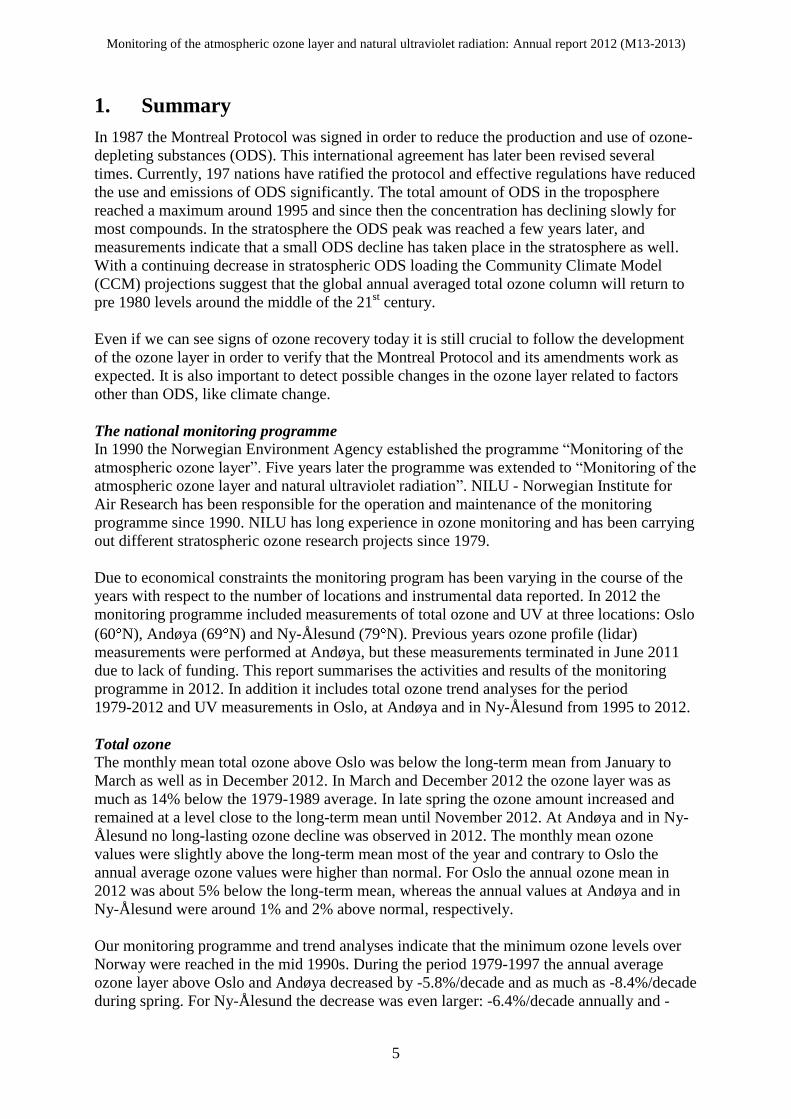
Recovery of the ozone layer is a process beginning with a decrease in the rate of decline,

followed by a levelling off and finally an increase in ozone driven by the changes in the

concentrations of ozone-depleting substances.

Figure 4: Total ozone at latitudes 60°N to 60°S for the period 1960 to 2100 (the x-axis is

not to scale). The thick red line is a representation of the ozone amounts observed to date

and projected for the future. The red-shaded region represents the model results predicted

for the future. The 1980 ozone level benchmark is shown as the horizontal line. The dashed

thick grey line represents the 1960 levels. Three recovery stages are shown by dashed

green ellipses (Figure from WMO, 2011).

Figure 4 is taken from the assessment report and shows a schematic diagram of the temporal

evolution of global ozone amounts beginning with pre-1980 values. This represents a time

before significant ozone depletion occurred due to emission of anthropogenic ozone depleting

substances (ODS). The thin black curve represents ground based observations averaged over

60⁰S-60⁰N, whereas the thin coloured curves represent various satellite observations. The

thick red line is a representation of the ozone amounts observed to date and projections for the

future, where three stages of recovery are marked by the green dashed ellipses. The red-

shaded region represents the model predictions for the future. It is worth noting that the range

is rather large and that both an under-recovery and a “super-recovery” are possible. Because

of factors other than ODSs, the ozone levels in the future could easily go above the values that


14

were present in the 1980s or even the 1960s ("super-recovery"). This is not recovery from the

influence of ODSs but due to other factors, primarily changes in CO2. Therefore, the term

"super-recovery" differs from references to recovery from ODS-forced ozone depletion.

The 2006 Assessment (WMO, 2007) showed that the globally averaged total ozone column

stopped declining around 1996, meeting the first criteria in the stage of recovery. The next

decades the ozone layer is expected to increase as a result of continued decrease in ODSs.

According to the last Assessment report (WMO, 2011) the total global ozone amount has not

started to increase yet, but has been fairly stable the last years. The average total ozone for the

period 2006–2009 remain at the same level as for previous period, i.e. roughly 3.5% and 2.5%

below the 1964–1980 averages for 90°S–90°N and 60°S–60°N, respectively.

The most dramatic ozone depletion has occurred in the Polar Regions. This region also

exhibits the highest level of natural variability, which makes the predictions of recovery more

uncertain. In Antarctica the ozone layer continues to reach very low levels from September to

November. In the Arctic and at high northern latitudes the situation is more irregular as severe

springtime ozone depletion usually occurs in years where the stratospheric temperatures are

low, exemplified with the different situations in spring 2012 (high ozone values) and the

record minimum levels in spring 2011 (not a part of the WMO report).

In the Arctic region the rate of recovery will partially depend on possible dynamical and

temperature changes the coming decades, both in the stratosphere as well as the troposphere.

The Arctic winter and springtime ozone loss between 2007 and 2012 has been variable, but

has remained in a range comparable to the values prevailing since the early 1990s. Model

predictions indicate that the evolution of ozone in the Arctic is more sensitive to climate

change than in the Antarctic. The projected strengthening of the stratospheric circulation in

Arctic is expected to increase lower stratospheric ozone transport and speed up the return to

1980 levels.

The ozone levels in the Arctic and high northern latitudes will also be strongly influenced by

changes in stratospheric winter temperatures during the next years, and possibly result in

delayed recovery or record low ozone observations due to formation of PSCs. Considerably

longer data series and improved understanding of atmospheric processes and their effect on

ozone are needed to estimate future ozone levels with higher confidence.

Studies of long-tem ozone trend, presented in the next sections, are essential in the assessment

of possible ozone recovery and to gain more information about atmospheric processes.

3.2 Trends for Oslo 1979 – 2012

Total ozone measurements using the Dobson spectrophotometer (No. 56) were performed on

a regular basis in Oslo from 1978 to 1998. The complete set of Dobson total ozone values

from Oslo is available at The World Ozone Data Centre, WOUDC (http://www.msc-

smc.ec.gc.ca/woudc/). Since the summer 1990 Brewer instrument no. 42 has been in

operation at the University of Oslo. The entire set of Brewer DS measurements from Oslo has

also been submitted to The World Ozone Data Centre.

Overlapping measurements of Dobson and Brewer total ozone in Oslo from 1990 to 1998

have shown that the two instruments agree well, but there is a systematic seasonal variation in

the difference between the two instruments. Thus, a seasonal correction function has been

http://www.msc-smc.ec.gc.ca/woudc/

http://www.msc-smc.ec.gc.ca/woudc/


15

applied to the entire Dobson ozone time series from 1978 to 1998. The homogenized Oslo

time series has been used in all ozone analyses presented in this report.

Figure 5a shows the variations in

monthly mean ozone values in Oslo

for the period 1979 to 2012. The

large seasonal variations are typical

for stations at high latitudes. This is a

dynamic phenomenon and is

explained by the springtime transport

of ozone from the source regions in

the stratosphere above the equator.

In order to make ozone trend

analyses for the period 1979 – 2012

we have removed the seasonal

variations by subtracting the long-

term monthly mean ozone value from

the data series, shown in Figure 5b.

Next, we have divided the time series

into two periods: 1) 1978-1997, and

2) 1998-2012. For the first time

period the ozone measurements were

entirely derived from the Dobson

instrument and reflect a time period

where a gradual decline in

stratospheric ozone was observed at

most mid and high latitude stations.

The second period has been based on

Brewer measurements, with

inclusion of some GUV measure-

ments. For the two time periods

simple linear regression lines have

been fitted to the data to describe

trends in the ozone layer above Oslo.

The results are summarized in

Table 4. The numbers in the table

represent seasonal and annual

percentage changes in total ozone (per decade) for the two time periods. The numbers in

parenthesis gives the uncertainty (1 ) in percent/decade. A trend larger than 2 is considered

to be significant. In winter and spring the ozone variability is relatively large and the

corresponding ozone trend must be large in order to be classified as statistical significant.

The second column in Table 4 indicates that a large ozone decrease occurred during the 1980s

and first half of the 1990s. For the period 1979-1997 there was a significant decline in total

ozone for all seasons. For the winter and spring the decrease was as large as -6.2 %/decade

and -8.4 %/decade, respectively. The negative ozone trend was less evident for the summer,

but nevertheless it was significant to a 2 level.

Figure 5a: Time series of monthly mean total ozone

in Oslo 1979-2012.

Figure 5b: Variation in total ozone over Oslo for the

period 1979–2012 after the seasonal variations have

been removed. Trend lines are marked in red.


16

For the period 1998-2012 the picture is different. There are substantial annual fluctuations one

should be cautious to draw any definite conclusions about trends. Nevertheless, the regression

analysis gives a good indication of the status of the ozone layer for recent years. As seen from

the last column in Table 4 none of the trend results are significant to a 2 level. For the

summer months there is an ozone decline of -1.6% /decade during the last 15 years, whereas

the ozone trend is correspondingly positive (+2.3%/decade) for the fall. The total ozone was

very low most of 2011 and the winter 2012, which has strongly affected the 1998-2012 trend

results. For example, the ozone winter trend from 1998-2010 was as large as +4.5%/ decade.

When 2011 and 2012 was included in the trend analysis the positive winter trend turned to a

negative value of -0.9%/ decade. This clearly demonstrates how trend results can be affected

by extreme values in the start and/or end of a short regression period. As seen from Table 4

the annual ozone trend from 1998 to 2012 is close to zero.

Table 4: Percentage changes in total ozone per year for Oslo for the period 1.1.1979 to

31.12.2012. The numbers in parenthesis gives the uncertainty (1 ) in percent. Data from the

Dobson and Brewer instruments have been used in this study. A trend larger than 2 is

considered to be significant.

Season Trend (% /decade) 1979-1997

Trend (% /decade) 1998-2012

Winter (Dec – Feb) -6.2 (2.4) -0.9 (3.0)

Spring (Mar – May) -8.4 (1.4) -0.8 (2.5)

Summer (Jun – Aug) -3.4 (1.1) -1.6 (1.3)

Fall (Sep – Nov) -4.3 (1.0) 2.3 (1.6)

Annual (Jan – Dec): -5.8 (1.0) -0.5 (1.4)

3.3 Trends for Andøya 1979–2012

The Brewer instrument has been in operation at Andøya since 2000. In the period 1994 to

1999 the instrument was located in Tromsø, approximately 130 km North of Andøya. Studies

have shown that the ozone climatology is very similar at the two locations (Høiskar et al.,

2001), and the two datasets are considered equally representative for the ozone values at

Andøya. For the time period 1979–1994 total ozone values from the satellite instrument

TOMS (Total ozone Mapping Spectrometer) have been used for the trend studies.

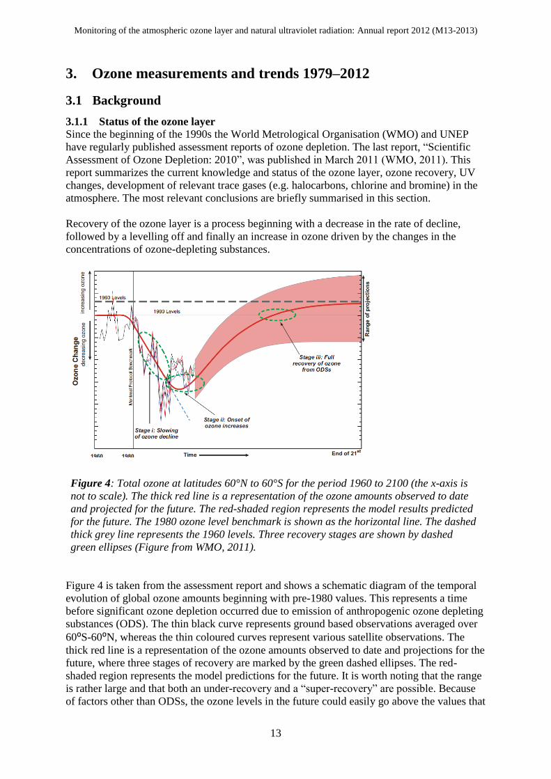
Figure 6a shows variation in the monthly mean ozone values at Andøya from 1979 to 2012.

The extreme February 2010 value and the record low 2011 spring values are seen as high and

low peaks in the plot. The variations in total ozone at Andøya for the period 1979–2012, after

removing the seasonal variations, are shown in Figure 6b together with the annual trends.

October – February months are not included in the trend analysis due to lack of data and

uncertain ozone retrievals during seasons with low sun. Simple linear regression lines have

been fitted to the data in Figure 6b. Similar to the Oslo site we have chosen to divide the

ozone time series into two periods: 1) 1979-1997, and 2) 1998-2012. The results of the trend

analyses are summarized in Table 5. Comparison of Figure 5b and Figure 6b shows that the

trend patterns from Andøya have many similarities to the Oslo trend pattern.


17

Similar to Oslo, the ozone layer

above Andøya declined

significantly from 1979 to 1997.

This decline is evident for all

seasons. The negative trend for the

spring season was as large as -8.4

%/decade, whereas the negative

trend for the summer months was -

2.8%/decade. The yearly trend in

total ozone was -5.8%/decade. In

contrast, no significant trends were

observed for the second period

from 1998 to 2012. For this period

an ozone decrease of -0.7%/decade

was observed for the spring,

whereas a trend of -0.8%/decade

was found for the summer months.

The annual trend for the period

1998-2012 was -0.2% /decade.

None of these results are significant

at either 1 or 2 significance

level.

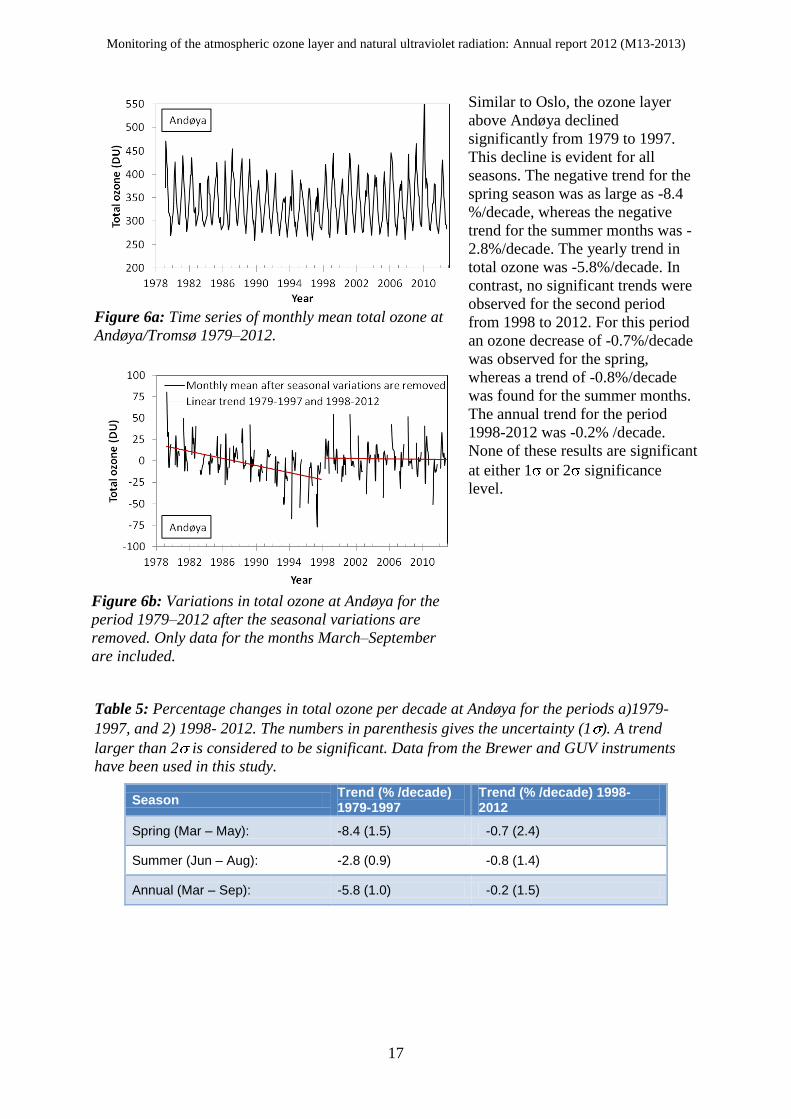
Table 5: Percentage changes in total ozone per decade at Andøya for the periods a)1979-

1997, and 2) 1998- 2012. The numbers in parenthesis gives the uncertainty (1 ). A trend

larger than 2 is considered to be significant. Data from the Brewer and GUV instruments

have been used in this study.



Spring (Mar – May): -8.4 (1.5) -0.7 (2.4)

Summer (Jun – Aug): -2.8 (0.9) -0.8 (1.4)

Annual (Mar – Sep): -5.8 (1.0) -0.2 (1.5)

Figure 6a: Time series of monthly mean total ozone at

Andøya/Tromsø 1979–2012.

Figure 6b: Variations in total ozone at Andøya for the

period 1979–2012 after the seasonal variations are

removed. Only data for the months March–September

are included.


18

3.4 Trends for Ny-Ålesund 1979 – 2012

The first Arctic ozone measurements started in Svalbard more than 60 years ago. In 1950 a

recalibrated and upgraded Dobson instrument (D8) was sent to Longyearbyen, and Søren

H.H. Larsen was the first person who performed ozone measurements in polar regions

(Henriksen and Svendby, 1997).

Larsen studied the annual ozone

cycle, and his measurements were

of great importance when Gordon

M.B. Dobson and his co-workers

went to Antarctica (Halley Bay)

some years later.

Regular Dobson ozone

measurements were performed at

Svalbard until 1962. The data have

been reanalyzed and published by

Vogler et al. (2006). After 1962

only sporadic measurements were

performed in Longyearbyen, but

after the instrument was moved to

Ny-Ålesund in 1994 more

systematic measurements took

place. However, the Dobson

instruments require manual

operation and it soon became more

convenient to replace the manual

instrument with the more automatic

SAOZ and GUV instruments.

The ozone measurements presented

in Figure 7a and Figure 7b are

based on a combination of Dobson,

SOAZ, GUV and satellite

measurements. For the years 1979

to 1994 the monthly mean ozone

values are entirely based on TOMS

Nimbus 7 and Meteor-3 overpass data. For the latest 20 years only ground based

measurements are used: Dobson data are included when available, SAOZ data are the next

priority, whereas GUV data are used when no other ground based measurements are available.

As seen from Figure 7b and Table 6 the trend pattern in Ny-Ålesund has many similarities to

the Oslo and Andøya trend series. A massive ozone decline was observed from 1979 to 1997,

especially during winter and spring. The negative trend for the spring season was as large as

-11.4%/decade, whereas the negative trend for the summer months was only -1.0%/decade.

The annual trend in total ozone was -6.4%/decade during these years. In contrast, no

significant trends were observed for the second period from 1998 to 2012. During this period

an ozone decrease of -1.9%/decade was observed for the spring months, whereas a trend of

Figure 7a: Time series of monthly mean total ozone at

Ny-Ålesund 1979–2012.

Figure 7b: Variations in total ozone at Ny-Ålesund for

the period 1979–2012. Only data for the months

March–September are included.


19

+1.2%/decade was found for the summer months. The annual trend for the period 1998-2012

was -0.7% /decade. None of these results are significant at either 1 or 2 significance level.

Table 6: Percentage changes in total ozone per decade in Ny-Ålesund for the periods

a) 1979-1997, and 2) 1998- 2012. The numbers in parenthesis gives the uncertainty (1 ). A

trend larger than 2 is considered to be significant.



Spring (Mar – May): -11.4 (1.8) -1.9 (3.3)

Summer (Jun – Aug): -1.0 (1.3) 1.2 (1.6)

Annual (Mar – Sep): -6.4 (1.1) -0.7 (2.0)

3.5 The overall ozone situation for Norway 2012

The ozone pattern and month-to-month variations at the three Norwegian sites were slightly

differently in 2012. The overall Norwegian ozone picture was not as dramatic as in 2011,

when record low ozone values in March and April contributed to low values throughout the

rest of the year. In spite of low ozone values in Oslo in January-March 2012, the weather

frontal systems changed in April and resulted in ozone values close to the long term-mean rest

of the year. Figure 8 shows a map from WOUDC 15 March 2012 illustrating ozone deviations

at the Northern Hemisphere. This day the ozone decline in Southern Norway was 20-25%,

whereas insignificant reductions where measured at Andøya and Ny-Ålesund. This was a

typical situation winter and early spring 2012.

Figure 9, Figure 10 and Figure 11 show the percentage difference between yearly mean total

ozone and the long-term yearly mean for all years from 1979 to 2012. The low values in 1983

and 1992/1993 are related to the eruption of the El Chichón volcano in Mexico in 1982 and

the Mount Pinatubo volcano at the Philippines in 1991. Also, the low ozone values in 2011

can clearly be seen.

For Oslo the annual ozone mean in 2012

was about 5% below the long-term mean.

As explained above the low ozone average

was caused by the unusual low values

during the winter months. Contrary to Oslo,

the annual average ozone values at Andøya

and in Ny-Ålesund were above the long-

term mean in 2012: around 1% and 2% for

the two stations, respectively.

Figure 8: Deviation from normal ozone

values 15 March 2012 (map from

WOUDC).


20

Figure 9: Percentage difference between yearly mean total ozone in Oslo and the long-term

yearly mean for 1979-1989.

Table 7 gives the percentage difference between the monthly mean total ozone values for

2012 and the long-term monthly mean values for the three Norwegian sites. For Oslo the

ozone level was as large as 14% below “normal” in March and December. Only June and

November 2012 had values above the long-term average. At Andøya all the 2012 values were

within ±5% compared to the long-term mean. The largest negative deviation was seen in

August (-2.9%), whereas the largest positive deviation occurred in April (+4.3%). In

Ny-Ålesund the ozone level was fairly high most of the year. In August the monthly mean

value was as much as 8.5% above than the 1979-1989 average. As noted in Section 2.3 the

high Ny-Ålesund values can partly be assigned the fact that GUV ozone values in general are

higher than the satellite retrieved ozone values, which have been used for calculating the

ozone long-term mean for the 1979-1989 period. This will be described in more detail in

Section 4.

Figure 10: Percentage difference between yearly mean total ozone at Andøya and the long-

term yearly mean for 1979-1989 for the months March-October.


21

Again, comparison of Figure 9, Figure 10 and Figure 11 shows that the ozone patterns at the

three Norwegian sites have several similarities. At all sites high ozone values were measured

in the end of the 1970s and in 2010. Also, all sites had record low ozone values in 1993

(around 9% below the long-term 1979-1989 mean) and low ozone values in 2011 (roughly

6% below the long-term yearly mean).

Figure 11: Percentage difference between yearly mean total ozone in Ny-Ålesund and the

long-term yearly mean value (1979-1989 average). Ozone values from March to October are

included in the calculations.

Table 7: Percentage difference between the monthly mean total ozone values in 2012 and the

long-term mean for Oslo, Andøya, and Ny-Ålesund.

Month Oslo (%) Andøya (%) Ny-Ålesund (%)

January -11.4

February -12.6 -2.1 -2.0

March -14.1 0.2 -4.0

April -1.4 4.3 1.7

May -5.6 2.8 6.3

June 2.0 1.5 4.0

July -0.9 2.7 8.5

August -2.4 -2.9 2.2

September -0.8 -1.7 0.3

October -1.1 -0.6 1.7

November 3.2

December -14.4


22

4. Satellite observations of ozone above Norway and the

Norwegian Arctic region

Satellites can never replace our ground based ozone monitoring network, but they give a very

important contribution to the global ozone mapping. For Norway and the Norwegian Arctic

region the use of satellite data will provide valuable information on spatial distribution of

ozone and UV radiation. Satellites also make it possible to investigate the geographical extent

of low ozone episodes during spring and summer and thereby discover enhanced UV intensity

on a regional level. Based on projects jointly financed by The Norwegian Space Centre (NRS,

Norsk Romsenter) and NILU we are in a good position to explore and utilize ozone satellite

observations in the National monitoring of the ozone and UV radiation. One project

(SatMonAir) was funded in 2012, whereas a follow-up project (SatMonAir II) started in 2013.

Some results from the activities within the SatMonAir projects are included in this report.

4.1 Short introduction to ozone observations from space

The amount and distribution of

ozone in the stratosphere varies

greatly over the globe and is mainly

controlled by two factors: the fact

that the maximum production of

ozone takes place at 40 km height in

the tropical region, and secondly the

large scale stratospheric transport

from the tropics towards the mid-

and high latitudes. In addition there

are small scale transport and

circulation patterns in the

stratosphere determining the daily

ozone levels. Thus, observing ozone

fluctuations over just one spot is not

sufficient to give a precise

description of the ozone situation in

a larger region. Satellite

observations are filling these gaps.

However, satellite observations rely on proper ground based monitoring as satellites have

varying and unpredictable life times, and calibration and validation rely upon high quality

ground based observations. Thus satellite observations are complementary to ground based

observations, and both are highly necessary.

Observations of seasonal, latitudinal, and longitudinal ozone distribution from space have

been performed since the 1970’s, using a variety of satellite instruments. The American

institutions NASA and NOAA (National Oceanic and Atmospheric Administration) started

these observations, and later The European Space Agency initiated their ozone programmes.

Figure 12 gives an overview of the various ozone measuring satellites and their time.

Figure 12: An overview of the various satellites and

their instruments measuring ozone from space since

the beginning of 1970’s (Figure from NASA).

Year


23

4.2 Satellite ozone observations above the Norwegian sites 1979–2012

In the course of the last 35 years several satellites have provided ozone data for Norway. The

most widely used instruments have been TOMS (onboard Nimbus-7), TOMS (onboard

Meteor-3), TOMS (on Earth Probe), GOME I (on ESR-2), GOME-2 (on MetOp),

SCIAMACHY (on Envisat), and OMI (onboard Aura). In the 1980s TOMS Nimbus 7 was the

only reliable satellite borne ozone instrument in space, but the last decades overlapping ESA

and NASA satellite products have been available. Also, different ozone retrieval algorithms

have been used over the years, which have gradually improved the quality and confidence in

the ozone data. Corrections for instrumental drift and increased knowledge of ozone

absorption cross sections and latitude dependent atmospheric profiles have improved the data

quality, especially in the Polar region.

In 2011 the Arctic ozone situation was extraordinary in winter/spring, where extremely low

ozone values were measured until the beginning of April. Figure 13 (left panel) shows the

Scandinavian/Arctic ozone situation 1st April 2011, with ozone values down to 250 DU north

of 70ºN. As shown in Figure 13 (right panel) the ozone situation was very different 1st April

2012, where ozone values around 500 DU were measured in Arctic regions. The ground based

ozone values in Oslo, at Andøya and in Ny-Ålesund are marked in the figures (blue numbers)

along with the OMI ozone value at the same locations (black numbers).

Comparisons of Ground based measurements and satellite data over Oslo, Andøya and

Ny-Ålesund show that the satellite values normally differs from the ground based measure-

ments. Ozone can exhibit some variations within short distances and a satellite pixel of

typically 1x1 degree might have an average value that deviates from the point measurement.

On the other hand the satellites give a very good picture of spatial extent of “ozone holes” and

how ozone rich/poor air moves. As a part of the SatMonAir projects spatial correlation,

standard deviation and bias between satellite products (plus comparisons to ground based

measurements) have been studied.

Figure 13: Ozone maps over Scandinavia and the Arctic 1st April 2011 (left panel) and

1st April 2012 (right panel). The numbers above Oslo, Andøya and Ny-Ålesund represent

satellite observations (black) and ground based observation (blue numbers).


24

As mentioned above, there might be relative large differences between ground based

measurements and satellite retrieved data on a day-to-day basis. In addition there are often

differences between the various satellite ozone products for overlapping time periods. The

differences have regional, seasonal and systematic nature.

Figure 14: Difference between ground based (GB) and satellite retrieved monthly mean

ozone values from 1979 to 2012 (Oslo) and 1995-2012 (Andøya and Ny-Ålesund). Deviations

(GB minus satellite values) are given in %. Upper panel: Oslo, Middle panel: Andøya, Lower

panel: Ny-Ålesund.


25

The monthly mean ozone values from ground based (GB) measurements and satellites are

analysed for the full period 1979-2012. Figure 14 shows the percentage GB-Satellite

deviation in Oslo (upper panel), at Andøya (middle panel) and in Ny-Ålesund (lower panel)

for different satellite products. Monthly mean ozone values are calculated from days where

simultaneous ground based and satellite data are available. The most surprising finding is that

the monthly mean ozone deviation between two different satellites can be up to 15%, e.g. in

December 2004 where OMI measured 328 DU and SCIAMACHY measured 380 DU, a

difference of 52 DU. The ground based Brewer observation was 329 DU this month, which

was close to the OMI ozone value. This clearly demonstrates the importance of continuous

long-term ground based measurements.

Table 8: Average deviations in % between ground based and satellite retrieved monthly mean

ozone values from Oslo and Andøya. Standard deviation and variance are also included.

Oslo

Instrument Period Mean St. Dev Variance

TOMS (Nimbus 7) Nov-78 May-93 1.35 1.88 3.53

TOMS (Earth probe) Jul-96 Dec-05 0.96 1.60 2.56

OMI Oct-04 Dec-12 0.98 1.40 1.96

GOME I Mar-96 Jul-11 -0.85 2.42 5.84

GOME II Jan-07 Dec-12 0.91 1.77 3.12

SCIAMACHY Jul-02 Apr-12 -2.07 4.43 19.63

Andøya



OMI Oct-04 Oct-12 2.64 2.09 4.36

GOME 1 Mar-96 Jul-11 1.42 2.78 7.74

GOME 2 Jan-07 Dec-12 2.12 2.02 4.10

SCIAMACHY Jul-02 Apr-12 0.30 2.37 5.61

Ny-Ålesund



OMI Oct-04 Dec-12 2.51 4.18 17.45

GOME 1 Mar-96 Jul-11 1.18 3.78 14.30

GOME 2 Jan-07 Dec-12 3.14 3.45 11.93

SCIAMACHY Jul-02 Apr-12 -0.67 4.86 23.61

Table 8 gives an overview of the average deviations between ground-based ozone

measurements and various satellite data products, together with standard deviations and

variance for Oslo, Andøya and Ny-Ålesund. For Oslo, ozone values from TOMS, OMI and

GOME II seems to be slightly underestimated, whereas GOME I and SCIAMACHY tend to

overestimate the ozone. For Andøya all mean satellite values are lower than the ground based

observations. The same is the case in Ny-Ålesund, except from SCIAMACHY which has a

large negative bias during early spring and late fall which gives an overall annual average

ozone value higher than the ground based mean value. For Ny-Ålesund, all satellite retrieved


26

ozone values are lower than the ground based measurements during summer. As seen from

Figure 14 (lower panel), the GB measurements are typically 7-8% higher during the summer

months. This might be caused by overestimated GUV ozone values, but can also be attributed

to uncertain satellite retrievals at high latitudes. Comparisons to other ground based

instruments, preferably Dobson or Brewer measurements, will give a better insight to this

problem.

There are also clear seasonal variations in the deviations between GB ozone and satellite

retrieved ozone values, especially in Oslo and Ny-Ålesund. For example, SCIAMACH

systematically overestimates ozone values during periods with low sun. This gives a very high

standard deviation and variance for the GB-SCIAMACHY deviation in Oslo and Ny-Ålesund.

The high SCIAMACHY winter values are visualized by the light blue columns/lines in

Figure 14. In contrast the OMI ozone values are close to the Brewer measurements in Oslo all

year, giving a variance of only 2.0 (see Table 8). The GB-OMI variance in Ny-Ålesund is as

high as 17.5, whereas GB-GOME II has a variance of only 11.9. This might indicate that

GOME II is more accurate at high latitudes. It can also be noted that the BG-SCIAMACHY

variance is much smaller at Andøya than in Oslo. This is probably caused by the fact that no

measurements are performed in December, January and most of November and February.

Thus, the months with largest uncertainty and variance are omitted from the comparison.

One aim of the SatMonAir project is to define and construct an integrated satellite data set

that is suitable for trend analysis for the Scandinavian region. Based on the analysis and

results presented in Table 8 it can be concluded the ozone data from TOMS and OMI have

similar mean and standard deviation and are suited for such trend studies, especially in

Southern Norway. Figure 15 shows the results from our preliminary satellite trend

calculations, focusing on April isolated. Left panel shows trends from 1979-1993, where a

large negative trend of 7- 10%/decade is seen most places in Norway. This is in line with

trend results presented in Section 3.2 - 3.4. However, for the westerly regions around Iceland,

the negative trend is less evident. For the period 1998-2012 no strong satellite retrieved ozone

trend is seen in the Arctic regions. For the Svalbard and Andøya area the trend is close to

zero, whereas a negative trend of around 3%/decade can be seen around Oslo. For the Bergen

region the negative 1998-2012 April trend is somewhat larger and estimated to about

7%/decade.

Figure 15: April ozone trend (%/decade) calculated from space. Left panel: TOMS Nimbus 7

data 1979-1993. Right panel: TOMS Earth Probe and OMI data 1998-2012.

1979-1993


27

5. Coupling of stratospheric ozone and climate

Climate change will affect the evolution of the ozone layer in several ways; through changes

in transport, chemical composition, and temperature (IPCC, 2007; WMO, 2007). In turn,

changes to the ozone layer will affect climate through the influence on the radiative balance,

and the stratospheric temperature gradients. Climate change and the evolution of the ozone

layer are coupled, and understanding of the processes involved is very complex as many of

the interactions are non-linear.

Radiative forcing1 is a useful tool to estimate the relative climate impacts due to radiative

changes. The influence of external factors on climate can be broadly compared using this

concept. Revised global-average radiative forcing estimates from the 4th

IPCC are shown in

Figure 16 (IPCC, 2007). The estimates are for changes in anthropogenic factors since pre-

industrial times. Stratospheric ozone is a greenhouse gas. The change in stratospheric ozone

since pre-industrial times has a weak negative forcing of -0.05 W/m2 with a medium level of

scientific understanding. This new estimate is weaker than in the previous report where the

estimate was –0.15 W/m2. The updated estimate is based on new model results employing the

same data set as in the previous report, where observational data up to 1998 is included. No

study has utilized ozone trend observations after 1998 (Forster et al., 2007).

Figure 16: Global-average radiative forcing estimates for important anthropogenic agents

and mechanisms as greenhouse gases, aerosol effects, together with the typical geographical

extent (spatial scale) of the forcing and the assessed level of scientific understanding (LOSU).

1 Radiative forcing is a measure of the influence a factor has in altering the balance of incoming and outgoing energy in the

Earth-atmosphere. It is an index of the importance of the factor as a potential climate change mechanism. It is expressed in

Wm-2 and positive radiative forcing tends to warm the surface. A negative forcing tends to cool the surface.


28

The temporarily and seasonally non-uniform nature of the ozone trends has important

implications for the radiative forcing. Total column ozone changes over mid latitudes is

considerable larger at the southern hemisphere (-6%) than at the northern hemisphere (-3%).

According to the IPCC report the negative ozone trend has slowed down the last decade, also

described in section 3 of this report.

Stratospheric ozone is indirectly affected by climate change through changes in dynamics and

in the chemical composition of the troposphere and stratosphere (Denman et al., 2007). An

increase in the greenhouse gases, especially CO2, will warm the troposphere and cool the

stratosphere. In general a decrease in stratospheric temperature reduces ozone depletion

leading to higher ozone column. However, there is a possible exception in the Polar Regions

where lower stratospheric temperatures lead to more favourable conditions for the formation

of more PSCs. These ice clouds are formed when the stratospheric temperature gets below -

78ºC. Chemical reactions occurring on the PSC surfaces can transform passive halogen

compounds into active chlorine and bromine and cause massive ozone destruction. This is of

particular importance in the Arctic region (WMO, 2007). It should also be mentioned that

ozone absorbs UV radiation and provides the heating responsible for the observed

temperature profile above the tropopause. Changes in stratospheric temperatures, induced by

changes in ozone or greenhouse gas concentrations will alter dynamic processes.

A long-term increase in stratospheric water content has been observed in the second half of

the 20th

century. This might have important consequences for the ozone layer as stratospheric

water vapour is among the main sources of OH in the stratosphere. OH is one of the key

species in the chemical cycles regulating the ozone levels. There are several sources for

stratospheric water, where CH4 is the most important. Other water vapour sources are

volcanoes and aircrafts, as well as natural and anthropogenic biomass burning which

indirectly can influence on stratospheric moisture through cloud mechanisms (Andreae et al.,

2004). In the 4th

IPCC report, the increase in stratospheric water vapour resulting from

anthropogenic emissions of methane (CH4) has a positive forcing of 0.07 W/m2, shown in

Figure 16.

The evolution of stratospheric ozone over the next decades will to a large extent depend on

the stratospheric halogen loading. Halocarbons play a double role in the ozone-climate

system. They are climate gases and contribute to a strong positive radiative forcing (see

Figure 16). In addition, chlorine and bromine containing compounds play a key role in ozone

destruction processes. Since ozone itself is an important climate forcer, less ozone means a

negative radiative forcing. The negative forcing due to the net ozone change from 1979 to

1994 has likely counterbalanced more than 30% of the positive forcing due to the increase of

well-mixed greenhouse gases in the same period (Hansen et al., 1997). However, if we study

radiative forcing related to human activities between 1750 and today (Figure 16), the ozone

depleting contribution is small compared with the contribution from all other greenhouse gas

increases.

Finally, nitrous oxide (N2O) is another key species that regulates the ozone levels. The

photochemical degradation of N2O in the stratosphere leads to ozone-depleting NOx.

Although the past emissions of ODSs (i.e. CFCs) still dominate global ozone depletion, the

current emission of N2O from human activities will destroy more stratospheric ozone than the

current emission of any ODS (WMO, 2011). Reduction of future N2O emissions, one target of

the Kyoto Protocol, would enhance the recovery of the ozone layer and would also reduce

anthropogenic forcing of the climate system.


29

6. UV measurements and levels

The Norwegian UV network was established in 1994/95 and consists of nine 5-channel GUV

instruments located from 58 N to 79 N, illustrated in Figure 17. NILU is responsible for the

daily operation of three of the instruments, located at Oslo (60 N), Andøya (69 N) and Ny-

Ålesund (79 N). The Norwegian Radiation Protection Authority (NRPA) is responsible for

the operation of the measurements performed at Trondheim, Bergen, Kise, Landvik, Finse and

Østerås. On-line data from the UV network is shown at www.nilu.no and at

http://www.nrpa.no/uvnett/.

This annual report includes results from

Oslo, Andøya and Ny-Ålesund. Due to lack

of funding, the GUV instrument in Ny-

Ålesund was omitted from the monitoring

programme in the period 2006-2009, but was

included again in 2010.

The Norwegian GUV instruments were

included in a calibration and intercomparison

campaign in 2005 as a part of the project

FARIN (Factors Controlling UV in

Norway)2. The project, which was financed

by The Norwegian Research Council, aimed

to quantify the various factors controlling

UV radiation in Norway. This includes e.g.

clouds, ozone, surface albedo, aerosols,

latitude, and geometry of exposed surface.

One part of the project has been the

comparison and evaluation of all the UV-

instruments in the Norwegian monitoring

network. In total 43 UV instruments were

included in the campaign. The three GUV

instruments from NILU were set up at

NRPA, Østerås, during the campaign and the

calibration results were satisfactory.

The GUV instruments are normally easy to maintain and have few interruptions due to

technical problems. The number of missing days due to technical problems in 2012 is given in

Table 9.

6.1 UV measurements in 2012

The UV dose rate is a measure of the total biological effect of UVA and UVB radiation (UV

irradiance weighted by the CIE action spectra). The unit for dose rate is mW/m2, but is often

given as a UV index (also named UVI). A UV index of 1 is equal to 25 mW/m2. The

2 http://www.nilu.no/farin/

Figure 17: Map of the stations included in

the Norwegian UV network. The stations

marked with blue are operated by NILU,

whereas the Norwegian Radiation Protection

Authority operates the stations marked with

green.

http://www.nilu.no/

http://www.nrpa.no/uvnett/


30

concept of UV index is widely used for

public information concerning sunburn

potential of solar UV radiation. At Northern

latitudes the UV indices typically vary

between 0 – 7 at sea level, but can range up

to 20 in Equatorial regions and high

altitudes (WHO, 2009). Table 10 shows the

UV-index scale with the recommended

protections at the different levels. The

recommendations are based on a moderate

light skin type, typical for the Nordic

population.

Table 10: UV-index together with the recommended protection.

UV-Index

Category Recommended protection

11+ Extreme Extra protection is definitively necessary. Avoid the sun and seek shade.

10

Very high Extra protection is necessary. Avoid the sun between 12 PM and 3 PM and seek shade. Use clothes, a hat, and sunglasses and apply sunscreen with high factor (15-30) regularly.

9

8

7 High

Protection is necessary. Take breaks from the sun between 12 PM and 3 PM. Use clothes, a hat, and sunglasses and apply sunscreen with high factor (15+). 6

5

Moderate Protection may be necessary. Clothes, a hat and sunglasses give good protection. Don't forget the sunscreen!

4

3

2 Low No protection is necessary.

1

Figure 18 shows the UV dose rates measured at noon (averaged between 10:30 and

11:30 UTC) for Oslo, Andøya and Ny-Ålesund. The highest UV dose rate in Oslo,

173.1 mW/m2, was observed 22 June at 11:17 UTC and is equivalent to a UV index of 6.9.

The black curves represent the measurements whereas the red curves are model calculations

employing the measured ozone values and clear sky. At Andøya the highest UV index in 2012

was 4.7, equivalent to a dose rate of 118.0 mW/m2, observed 24 June at 10:41 UTC. The

highest UVI value in Ny-Ålesund was 3.0, or 75.9 mW/m2, and was measured 16 June at

11:00 UTC. The maximum UVI in Oslo was observed during scattered cloud conditions and

slightly lower total ozone value than normal, i.e. 317 DU (normal ~ 340 DU). At Andøya the

ozone column was almost the same as in Oslo (311 DU versus normally ~ 350 DU) and was

measured during clear sky conditions. At Ny-Ålesund the maximum UVI was observed

during scattered cloud conditions and a total ozone column of 341 DU, slightly under the

normal of ~360 DU. For UV-levels corresponding to the maximum UVI-value of 6.9 in Oslo,

people with a typical Nordic skin type get sunburnt after approximately 20 minutes if no sun

protection is used.

Table 9: Number of days with more than

2 hours of missing GUV data in 2012 and

2011. Days where the sun is below the

horizon (polar night) are not included.

Station Technical problems

2012 2011

Oslo 1 1

Andøya 1 12

Ny-Ålesund 1 1


31

Figure 19 shows the atmospheric conditions during the days of maximum UVI in Oslo,

Andøya and Ny-Ålesund. A cloud transmission of 100% (red curve) represents clear sky

conditions. In Ny-Ålesund it was clear sky until noon and a few scattered clouds towards the

evening. As seen from Figure 19 (right

panel) the cloud transmission in Ny-

Ålesund was above 100% the first part

of the day. This was caused by high

albedo from snow and ice in the

vicinity of the instrument site, which

enhanced the solar radiation detected

by the GUV instrument. At Andøya the

day was fairly clear in the morning,

with a few scattered clouds around

noon. Such clouds tend to enhance the

UV-radiation due to scattering of

radiation towards the ground. Towards

the evening the sky became more and

more cloudy. Oslo had scattered clouds

all day, and this will normally create

multiple reflection which enhances the

UV-radiation.

Many people from Norway visit

Mediterranean countries during

holidays, and UV-indices may easily

become twice as high as in Oslo under

conditions with clear sky and low

ozone.

In Norway the highest UV dose rates

generally occur in the late spring and

early summer in alpine locations with

fresh snow, such as Finse in May and

early June. Here the UV indices at noon

can reach 8.

The seasonal variation in observed UV

dose rate is closely related to the solar

elevation. Consequently the highest UV

levels normally occur during the

summer months when the solar

elevation is highest. As mentioned

above the appearance of fresh snow in

late May and early June can enhance

the UV-level and give exceptional high

UV values. In addition to the solar

zenith angle, the UV radiation is

influenced by e.g. clouds, total ozone and ground reflection (albedo). Day-to-day fluctuation

in cloud cover is the main explanation for large daily variations in UV radiation. However,

rapid changes in the total ozone column, as may occur during the spring, may also give rise to

Figure 18: Hourly averaged UV dose rate

measured at noon (between 10:30 and 11:30 UTC)

in 2012. Upper panel: Oslo. Mid panel: Andøya

Lower panel: Ny-Ålesund.


32

large fluctuations in the UV-radiation. In general the UV-radiation in Ny-Ålesund is largely

enhanced during spring due to the high albedo from snow and ice that surrounds the

measurement site.

Figure 19: UV dose rates (left axis, black curves) and cloud transmission (right axis, red

curves) during the days of maximum UVI in Oslo (left panel), Andøya (middle panel) and

Ny-Ålesund (right panel). A cloud transmission of 100% represents clear sky conditions,

whereas cloud transmissions of 20-30% represent heavy clouds.

Monthly mean noon UV doses for Oslo, Andøya and Ny-Ålesund in 2012 are compared in

Figure 20. As expected, the monthly mean UV doses in Oslo were significantly higher than

the values observed at Ny-Ålesund, except for June when the midnight sun in Ny-Ålesund

contributes significantly to the UV-dose. If the cloud and ozone conditions at both sites were

similar during the summer, the UV-radiation would be highest in Oslo due to higher solar

elevation most of the day.

Figure 20: Monthly mean UV doses (in kJ/m

2) in 2012 measured with the GUV instruments

located in Oslo, Andøya and Ny-Ålesund.


33

6.2 Annual UV doses 1995 – 2012

Annual UV doses for the period 1995–2012 are shown in Table 11 for the GUV instruments

in Oslo, at Andøya and in Ny-Ålesund. Annual UV doses for 2005 are not included in the

Table as there were large gaps in the data set caused by a calibration campaign. The

uncertainty in the daily UV doses is estimated to 5 % at a 2 level (Johnsen et al., 2002). For

periods with missing data we have estimated the daily UV doses from a radiative transfer

model (FastRt, http://nadir.nilu.no/~olaeng/fastrt/fastrt.html). Normally this gives an

additional uncertainty in the annual UV doses of 1.6 % for all stations and years, except for

Andøya where the uncertainty is 2 % for 2000, 5 % for 2001, and 5 % for 2011 where

12 days of measurements are missing.

In 2012 the UV-doses in Oslo during summer were relative low. This can be explained by

many overcast days in June and July. As shown in Figure 18 (upper panel) there were many

days during the summer where the UV index in Oslo was below 2. Contrary to Oslo, there

were few heavy overcast days in Ny-Ålesund in 2012. Thus, the monthly mean UVI for June

is almost equal in Oslo and Ny-Ålesund (see Figure 20).

A graphical illustration of the yearly integrated UV-doses is shown in Figure 21 to show

yearly fluctuations.

Table 11: Annual integrated UV doses (in kJ/m2) for Oslo, Andøya and Ny-Ålesund for the

period 1995 – 2012.

Year Oslo (kJ/m

2)

Andøya (kJ/m

2)

Tromsø (kJ/m

2)*

Ny-Ålesund (kJ/m2)

1995 387.6

1996 387.4 253.6 218.5

1997 415.0 267.0 206.5

1998 321.5 248.4 217.7

1999 370.5 228.0 186.1

2000 363.0 239.7 231.0

2001 371.0 237.0 208.6

2002 382.5 260.0 201.8

2003 373.2 243.4 Excluded from the program

2004 373.2 243.7 190.5

2005 No annual UV doses due to gaps in the data caused by a calibration campaign





2010 360.5 225.6 201.6

2011 365.2 254.8 200.8

2012 352.6 227.5 211.6

*The GUV instrument at Andøya was operating at Tromsø in the period 1996 – 1999.

http://nadir.nilu.no/~olaeng/fastrt/fastrt.html


34

Figure 21: Annual integrated UV doses (in kJ/m2) at Oslo, Tromsø/Andøya and Ny-Ålesund

for the period 1995–2012.


35

7. References

Andreae, M.O., Rosenfeld, D., Artaxo, P., Costa, A.A., Frank, G.P., Longo, K.M., Silva-Dias,

M.A.F. (2004) Smoking rain clouds over the Amazon. Science, 303,1337-1342.

Denman, K.L., Brasseur, G., Chidthaisong, A., Ciais, P., Cox, P.M., Dickinson, R.E.,

Hauglustaine, D., Heinze, C., Holland, E., Jacob, D., Lohmann, U., Ramachandran, S., da

Silva Dias, P.L., Wofsy, S.C., Zhang, X. (2007) Couplings between changes in the climate

system and biogeochemistry. In: Climate Change 2007: The physical science basis.

Contribution of Working Group I to the fourth assessment report of the Intergovernmental

Panel on Climate Change. Ed. by S. Solomon, D. Qin, M. Manning, Z. Chen, M. Marquis,

K.B. Averyt, M.Tignor, H.L. Miller. Cambridge, Cambridge University Press.

Forster, P., Ramaswamy, V., Artaxo, P., Berntsen, T., Betts, R., Fahey, D.W., Haywood, J.,

Lean, J., Lowe, D.C., Myhre, G., Nganga, J., Prinn, R., Raga, G., Schulz, M., Van Dorland,

R. (2007) Changes in atmospheric constituents and in radiative forcing. In: Climate

Change 2007: The physical science basis. Contribution of Working Group I to the fourth

assessment report of the Intergovernmental Panel on Climate Change. Ed. by S. Solomon,

D. Qin, M. Manning, Z. Chen, M. Marquis, K.B. Averyt, M. Tignor, H.L. Miller.

Cambridge, Cambridge University Press.

Gröbner, J., Hülsen, G., Wuttke, S., Schrems, O., Simone, S. D., Gallo, V., Rafanelli, C.,

Petkov, B., Vitale, V., Edvardsen, K., Stebel, K. (2010) Quality assurance of solar UV

irradiance in the Arctic. Photochem. Photobiol. Sci., 9, 384-391.

Hansen, J., Sato, M., Ruedy, R. (1997) Radiative forcing and climate response, J. Geophys.

Res., 102, 6831-6864.

Henriksen, T., Svendby, T. (1997) Ozonlag, UV-stråling og helse. Department of Physics,

University of Oslo.

Høiskar, B.A.K., Braathen, G.O., Dahlback, A., Bojkov, B.R., Edvardsen, K., Hansen, G.,

Svenøe, T. (2001) Monitoring of the atmospheric ozone layer and natural ultraviolet

radiation. Annual report 2000. Kjeller (Statlig program for forurensningsovervåking.

Rapport 833/01. TA-1829/2001) (NILU OR 35/2001).

Høiskar, B.A., Braathen, G.O., Dahlback, A., Edvardsen, K., Hansen, G., Stebel, K.,

Svendby, T., Vik, A.F. (2003) Overvåking av ozonlaget og naturlig ultrafiolett stråling.

Årsrapport 2002. Kjeller (Statlig program for forurensningsovervåking. Rapport 881/2003)

(TA-1972/2003) (NILU OR 33/2003).

IPCC (2007) Summary for policymakers. In: Climate Change 2007: The physical science

basis. contribution of Working Group I to the fourth assessment report of the

Intergovernmental Panel on Climate Change. Ed. by S. Solomon, D. Qin, M. Manning,

Z. Chen, M. Marquis, K.B. Averyt, M.Tignor, H.L. Miller. Cambridge, Cambridge

University Press.

Johnsen, B., Mikkelborg, O., Hannevik, M., Nilsen, L.T., Saxebø, G., Blaasaas, K.G. (2002)

The Norwegian UV-monitoring program, period 1995/96 to 2001. Østerås, Statens

strålevern (Strålevern Rapport 2002:4).

Stamnes, K., Slusser, J., Bowen, M. (1991) Derivation of total ozone abundance and cloud

effects from spectral irradiance measurements. Appl. Opt., 30, 4418-4426.

Vogler, C., Bröonnimann, S., Hansen, G. (2006) Re-evaluation of the 1950–1962 total ozone

record from Longyearbyen, Svalbard. Atmos. Chem. Phys., 6, 4763-4773.


36

WHO (2009) Ultraviolet radiation and human health. Geneva, World Health Organization

(Fact Sheet No 305).

URL: http://www.who.int/mediacentre/factsheets/fs305/en/index.html.

WMO (2007) Scientific assessment of ozone depletion: 2006. Geneva, World Meteorological

Organization (Global Ozone Research and Monitoring Project – Report No. 50).

WMO (2011) Scientific assessment of ozone depletion: 2010. Geneva, World Meteorological

Organization, (Global Ozone Research and Monitoring Project – Report No. 52).

http://www.who.int/mediacentre/factsheets/fs305/en/index.html

Utførende institusjon NILU – Norsk institutt for luftforskning

ISBN-nummer 978-82-425-2600-7 (trykt)

978-82-425-2601-4

(elektronisk)

Oppdragstakers prosjektansvarlig Tove Marit Svendby

Kontaktperson

Miljødirektoratet Harold Leffertstra

M-nummer M13-2013

SPFO-nummer 1149/2013

År

2013

Sidetall 36

Miljødirektoratets (tidl.

Klif) kontraktnummer 4010021

Utgiver NILU – Norsk institutt for luftforskning

NILU OR 34/2013

NILU project no. O-106007/O-106008

Prosjektet er finansiert av Miljødirektoratet

Forfatter(e) T.M. Svendby, K. Edvardsen, C.L. Myhre, K. Stebel (all NILU), A. Dahlback (UiO)

Tittel - norsk og engelsk Overvåking av ozonlaget og naturlig ultrafiolett stråling: Årsrapport 2012.

Monitoring of the atmospheric ozone layer and natural ultraviolet radiation: Annual report 2012.

Sammendrag – summary Rapporten presenterer måledata for totalozon og UV-stråling over norske målestasjoner i 2012. For Oslo, Andøya

og Ny-Ålesund er trenden i totalozon beregnet for perioden 1979-2012. Ozonverdiene over Norge var tilnærmet

normale 2012, bortsett fra vinterverdiene i Oslo som var lavere enn normalt. Den klare reduksjonen av ozonlaget

over Norge i perioden 1979-1997 stoppet opp i 1998 og ozonlaget over Norge ser nå ut til å ha stabilisert seg.

This is an annual report describing the activities and main results of the monitoring programme “Monitoring of

the atmospheric ozone layer and natural ultraviolet radiation” for 2012. In 2012 the ozone values above Norway

were close to the long-term mean, except from the ozone winter values in Oslo which were lower than normal. A

clear decrease in the ozone layer above Norway during the period 1979-1997 stopped after 1998 and the ozone

layer above Norway now seems to have stabilized.

4 emneord Stratosfærisk ozon

UV-stråling

Målinger og observasjoner

Montreal-protokollen

4 subject words Stratospheric ozone

UV radiation

Measurements and observations

Montreal protocol

Om Statlig program for forurensningsovervåking

Statlig program for forurensningsovervåking omfatter

overvåking av forurensningsforholdene i luft og nedbør,

skog, vassdrag, fjorder og havområder. Overvåkings-

programmet dekker langsiktige undersøkelser av:

• overgjødsling

• forsuring (sur nedbør)

• ozon (ved bakken og i stratosfæren)

• klimagasser

• miljøgifter

Overvåkingsprogrammet skal gi informasjon om

tilstanden og utviklingen av forurensningssituasjonen,

og påvise eventuell uheldig utvikling på et tidlig

tidspunkt. Programmet skal dekke myndighetenes

informasjonsbehov om forurensningsforholdene,

registrere virkningen av iverksatte tiltak for å redusere

forurensningen, og danne grunnlag for vurdering av nye

tiltak. Miljødirektoratet er ansvarlig for

gjennomføringen av overvåkingsprogrammet.

SPFO-rapport 1149/2013

M13-2013

ISBN 978-82-425-2600-7 (trykt)

ISBN 978-82-425-2601-4 (elektronisk)

Miljødirektoratet

Telefon: 03400/73 58 05 00 | Faks: 73 58 05 01

E-post: [email protected]

Nett: www.miljødirektoratet.no

Post: Postboks 5672 Sluppen, 7485 Trondheim

Besøksadresse Trondheim: Brattørkaia 15, 7010 Trondheim

Besøksadresse Oslo: Strømsveien 96, 0602 Oslo

monitoring of the atmospheric ozone layer and natural ... · monitoring of the atmospheric ozone...

Documents