Money management with optimal stopping of losses for

maximizing the returns of futures trading1

Christian Lundström

Department of Economics

Umeå School of Business and Economics

Umeå University

SE-901 87 Umeå

Abstract

By using money management, an investor may determine the optimal leverage factor

to apply on each trade, for maximizing the profitability of investing. Research

suggests that the stopping of losses may increase the profitability of a trading strategy

when returns follow momentum. This paper contributes to the literature by

proposing the first money management criterion that incorporates optimal stopping

of losses. In an empirical trading study, we are able to substantially improve the

profitability when using this criterion, relative to the existing criteria. We conclude

that money management should incorporate stopping of losses when returns follow

momentum.

Key words: Kelly criterion, Vince optimal f, Leverage, Position size, Commodity trading advisor,

Managed futures hedge funds.

JEL classification: G11, G14, G17, G19.

1 The author thanks Kurt Brännäs, Tomas Sjögren, Jörgen Hellström, Daniel Halvarsson and André Gyllenram for

insightful comments and suggestions.

1

1. Introduction

Futures have become mainstream investment vehicles among traditional and alternative asset

managers (Fuertes et al., 2010). An investor may, through futures contracts, gain exposure to a

wide range of various asset classes such as commodities, fixed income, currencies, debt, and stock

market indices. Besides hedging, futures may be used as an inflation hedge (e.g., Greer, 1978;

Bodie and Rosansky, 1980; Bodie, 1983), and in portfolio diversification (e.g., Jensen et al., 2000;

Erb and Harvey, 2006). In addition, futures may be traded to generate abnormal returns (e.g.,

Chan et al., 2000; Jensen et al., 2002; Wang and Yu, 2004; Erb and Harvey, 2006; Miffre and Rallis

2007; Basu et al., 2010; Fuertes et al., 2010; Holmberg et al., 2013; Lundström, 2013). For example,

Erb and Harvey (2006) and Miffre and Rallis (2007) follow momentum signals to allocate capital

towards the best performing commodities and away from the worst performing ones. When

assessing the profitability of a publicly known day trading strategy, Holmberg et al. (2013) and

Lundström (2013) report empirical evidence of intraday momentum in futures contracts.

Futures trading for profit is a multi-billion US dollar industry. The Commodity Trading Advisor

(CTA) funds, or Managed Futures funds, constitute a particular class of hedge funds involved

solely in futures trading for profit. In 2013, CTA funds manage over 331 billion US dollars

(BarclayHedge.com 2014-04-10). Given abnormal returns in trading, the investor must, however,

decide what leverage factor he should apply on each trade. By using money management, an

investor may determine the optimal leverage factor to apply on each trade in order to maximize

the profitability of investing (e.g., Sewell, 2011). Money management is of immense importance

for an investor as it determines the difference between going broke and being extraordinarily

successful (e.g., Rotando and Thorp, 1992; Tharp, 1997; Williams, 1999, Faith, 2003; Anderson

and Faff, 2004; Tharp, 2007). To work well in investment applications, however, money

management requires a readily available supply of leverage. Adding to the appeal of futures is that

contracts may be bought on a margin.

In this paper we study money management for maximizing the profitability of futures trading.

There are two existing criteria in the literature (see MacLean et al., 2010; Sewell, 2011, for reviews)

from which we take our departure. First, Thorp (1969) extends the original Bernoulli game

criterion of Kelly (1956) on stock market and derivatives trading where the returns follow a

continuous probability distribution. In line with this literature, we denote this as the Kelly

criterion. The Kelly criterion is suggested for futures trading also by other authors (e.g., Gehm,

1983; Balsara, 1992; Poundstone, 2005). From a practical investment management perspective,

several of the most successful investors, including John Maynard Keynes, Warren Buffett, and

2

Bill Gross, use money management criteria similar to the Kelly criterion in their funds (see

Thorp, 1997; Ziemba, 2005; Ziemba and Ziemba, 2007, for details). Rotando and Thorp (1992)

study the empirical trading results from buying S&P 500 contracts at the start of the year, and

selling the same contracts at the end of the year. They find sizable long-run profitability when

reinvesting profits using the Kelly criterion, (Rotando and Thorp, 1992). Second, Vince (1990,

1992, 1995, 2009, 2011) independently suggests an alternative money management criterion for

futures trading; the optimal criterion. We refer to it as the Vince criterion to avoid confusion.

Anderson and Faff (2004) assess the profitability of a publicly available trading strategy in five

futures markets reinvesting profits using the Vince criterion. They conclude that money

management plays a more important role for profitability in futures trading than previously

realized, with large differences in profitability depending on what leverage factor is applied.

The stop loss is one of the most frequently used techniques to control futures market risk (e.g.,

Shyy, 1989) and considered an integral part of money management in futures trading among

practitioners (e.g., Tharp, 1997; Williams, 1999; Faith, 2003; Tharp, 2007). The stop loss is a

resting market order, tied to the opening price of the position, which covers the position if the

price moves by a distance against him. This distance is referred to as the stop distance and is

predetermined by the investor. Despite its popularity among practitioners, stopping of losses is

not part of the Kelly or Vince money management criteria, and the academic literature regarding

stop loss orders is limited. In the market microstructure literature, stop loss orders are somewhat

studied in the context of optimal order selection algorithms (e.g., Easley and O'Hara, 1991; Biais

et al., 1995; Chakravarty and Holden, 1995; Handa and Schwartz, 1996; Harris and Hasbrouck,

1996; Seppi, 1997; Lo et al., 2002). Shefrin and Statman (1985) and Tschoegl (1988) consider

behavioral patterns that may explain the popularity of stop loss orders among trading

practitioners. From this literature, stopping of losses can be seen as a mechanism for avoiding or

anticipating pitfalls of human judgment, e.g., the disposition effect and loss aversion. Kaminski

and Lo (2013) provide the first study of the stop loss effects on the profitability of a trading

strategy. They show that stop loss orders increase the profitability of trading if returns follow

momentum. The rationale is that if returns follow momentum, small losses tend to grow into

larger losses and, by stopping losses before they grow large, the stop loss should increase the

long-run profitability from trading. Kaminski and Lo (2013) furthermore finds empirical support

of an increase in trading profitability when stop loss orders are added to a buy and hold strategy

of a US equities index, using monthly returns data from January 1950 to December 2004.

3

As empirical evidence of momentum in returns are reported by many (e.g., Chan et al., 2000; Erb

and Harvey, 2006; Miffre and Rallis, 2007; Fuertes et al., 2010; Holmberg et al., 2013; Lundström,

2013) we expect that the stopping of losses should increase the profitability of many trading

applications (for momentum in the stock markets, see, for example, Jegadeesh and Titman, 1993).

Providing important insights of the stop loss effects on trading profitability, Kaminski and Lo

(2013) does not provide a criterion to determine the optimal stop distance, or analyze the

combined effects with optimal leverage by money management, in order to maximize the

profitability. A money management criterion that incorporates optimal stopping of losses should

be of interest to every investor trading for profit when returns follow momentum. Such a

criterion must, however, be able to account for both continuously distributed returns, but also

for discretely distributed returns of the stopped out trades.

This paper proposes the first money management criterion to incorporate optimal stopping of

losses in futures trading. The main contribution is that, by using the money management criterion

of this paper, the investor may increase the profitability of trading above that of the existing

criteria, when returns follow momentum. A minor contribution is that, although the Kelly and

the Vince criteria are treated as separate criteria, yielding possibly different profitability (e.g.,

Balsara, 1992; Tharp, 1997; Vince, 2011), we show in this paper that both criteria produce

identical profitability when evaluated under the same assumptions. To illustrate the practical

relevance of the proposed criterion of this paper, we apply it to a futures trading strategy together

with the Vince criterion. We are able to substantially improve the empirical profitability of futures

trading relative to the Vince criterion. We note that both the Kelly and Vince criteria are derived

assuming risk-neutral investors with the sole interest of maximizing the long-run profitability of

trading. To ensure comparability with the existing criteria, we therefore limit the study of this

paper to consider money management for risk-neutral investors only. Risk-averse investors

should instead apply only a fraction of the leverage factor suggested for maximizing the capital

growth, (see, MacLean et al., 2010, for a review).

The remainder of the paper is outlined as follows: In Section 2 we present the Kelly and Vince

criteria in futures trading. We propose the money management criterion with optimal stopping in

Section 3. In Section 4 we present the data and the empirical results, and Section 5 concludes.

4

2. Money management in futures trading

A trade position is initiated when an investor either buys, or short sells, a number of futures

contracts. The position is subsequently closed when the same contracts are covered, that is, sold

(bought) for a long (short) position. The decisions when to initiate a trade, and when to close the

trade, are determined by a trading strategy comprised of a given set of rules. In this paper we

consider any type of trading strategy. Strategies may be based on technical or fundamental

analysis, initiating long and/or short trades, for different assets, etc. Furthermore, we note that a

return from trading is generated over a time period which we refer to as the investment period.

The investment period may vary from seconds to several days, weeks, or possibly years,

depending on the strategy used. For reviews of various trading strategies, what rules they may be

comprised of, and the length of the investment periods, etc., see Conrad and Kaul (1998) and

Katz and McCormick (2000).

Suppose that is the return of trade , including trading costs, generated by a given trading

strategy. We assume, as with Thorp (1969) and Rotando and Thorp (1992), that the process { }

is stationary with a positive mean, , generated by a continuous returns distribution which is

exogenously given and a priori known. Moreover, we assume a risk-free interest rate equal to zero

and that money which is not used for trading remains at a constant value. When applying a fixed

leverage factor to capital, , on each trade , we may write the investor’s Terminal Wealth

Relative ( ) to the initial level of wealth, , as:

∏( )

( )

where is the wealth after successive trades. A leverage factor of , , or

corresponds to a smaller, equal, or larger exposure, respectively, relative to the capital

level. We assume as in Thorp (1969) and Rotando and Thorp (1992) that contracts are infinitely

divisible, yielding a continuous leverage factor, and that the investor chooses a small enough

leverage factor that satisfies: for each trade . We may thus write the growth rate of

capital as:

5

(

)

∑ ( )

( )

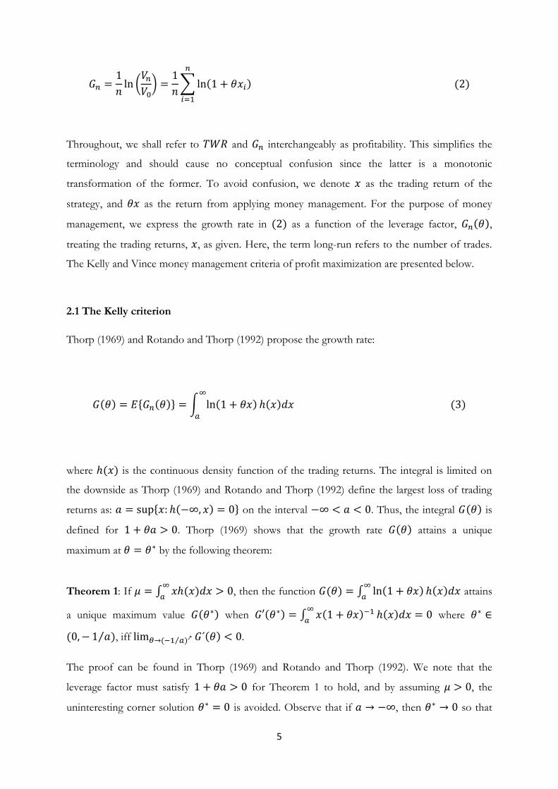
Throughout, we shall refer to and interchangeably as profitability. This simplifies the

terminology and should cause no conceptual confusion since the latter is a monotonic

transformation of the former. To avoid confusion, we denote as the trading return of the

strategy, and as the return from applying money management. For the purpose of money

management, we express the growth rate in ( ) as a function of the leverage factor, ( ),

treating the trading returns, , as given. Here, the term long-run refers to the number of trades.

The Kelly and Vince money management criteria of profit maximization are presented below.

2.1 The Kelly criterion

Thorp (1969) and Rotando and Thorp (1992) propose the growth rate:

( ) { ( )} ∫ ( )

( ) ( )

where ( ) is the continuous density function of the trading returns. The integral is limited on

the downside as Thorp (1969) and Rotando and Thorp (1992) define the largest loss of trading

returns as: { ( ) } on the interval . Thus, the integral ( ) is

defined for . Thorp (1969) shows that the growth rate ( ) attains a unique

maximum at by the following theorem:

Theorem 1: If ∫ ( )

, then the function ( ) ∫ ( )

( ) attains

a unique maximum value ( ) when ( ) ∫ ( )

( ) where

( ⁄ ), iff ( ⁄ ) ( ) .

The proof can be found in Thorp (1969) and Rotando and Thorp (1992). We note that the

leverage factor must satisfy for Theorem 1 to hold, and by assuming , the

uninteresting corner solution is avoided. Observe that if , then so that

6

the Kelly criterion applied to continuous distributions will yield non-trivial results only if the

lower limit of the integral ( ) ∫ ( )

( ) is finite, Rotando and Thorp (1992).

In fact, we note that the lower bound of any trading strategy return distribution is always limited

to as the price of the underlying asset can never attain values below zero. Therefore, we

consider here instead the largest loss: { ( ) } on the interval [ ).

The position size, , refers to the fraction of capital the investor stands to lose in each trade (e.g.,

Faith, 2003; Tharp, 2007). Thorp (1969) and Rotando and Thorp (1992) interpret as a leverage

factor, but refer to it as the fraction of capital to correspond to the original criterion by Kelly

(1956). This may be a somewhat confusing use of terminology as the Kelly criterion for futures

trading produces an optimal leverage on the interval ⁄ , not restricted to , while

the Kelly criterion for gambling produces an optimal position size, , on the interval of

(see Vince, 2011). The Vince criterion allows for this separation in futures trading.

2.2 The Vince criterion

Vince (1990, 1992, 1995, 2009, 2011) suggests that the investor should maximize the capital

growth rate with respect to the position size, relative to the largest loss of the trading returns.

Assuming that trading returns are of an a priori unknown distribution, Vince (1990, 1992, 1995,

2009, 2011) proposes that the investor should first estimate the returns distribution using

historical trading returns. We refer to the largest loss of the trading returns as ( ). The

Vince criterion then proposes the leverage factor: ( )

( ) | ( )|⁄ , where

indicates the Vince criterion. When applying the leverage factor, ( ), the largest loss of capital

is always limited to the position size: ( )

if ( ). The profitability, ( ), is

a function of in the Vince criterion, instead of as in the Kelly criterion.

We now compare the profitability of the Vince criterion with the Kelly criterion, and in the next

section with the criterion of this paper. For a fair comparison we compare the Kelly and Vince

criteria under the same assumptions. When we evaluate the Vince criterion under the

assumptions of this paper, the largest loss of is given by: { ( ) }, yielding

an optimal leverage factor of:

| |⁄ . Thus the Vince growth rate can be written as:

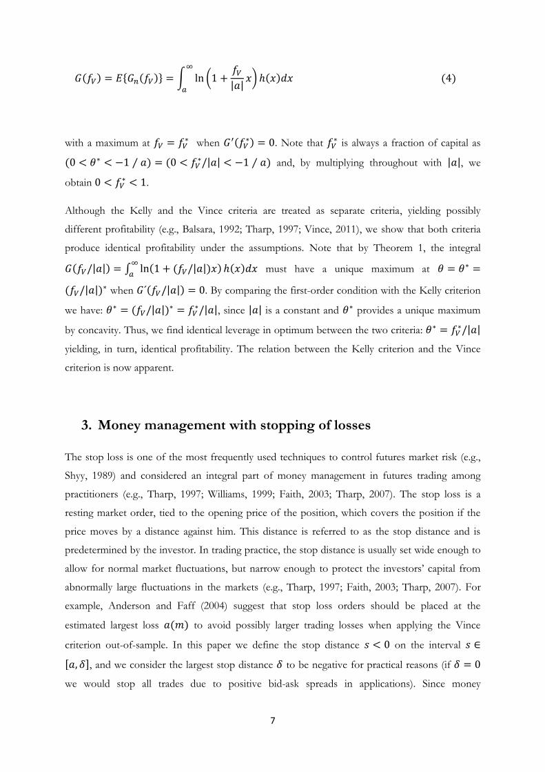
7

( ) { ( )} ∫ ( | |

)

( ) ( )

with a maximum at when (

) . Note that is always a fraction of capital as

( ⁄ ) ( | | ⁄ ) and, by multiplying throughout with | |, we

obtain .

Although the Kelly and the Vince criteria are treated as separate criteria, yielding possibly

different profitability (e.g., Balsara, 1992; Tharp, 1997; Vince, 2011), we show that both criteria

produce identical profitability under the assumptions. Note that by Theorem 1, the integral

( | |) ∫ ( ( | |) )

( ) must have a unique maximum at

( | |) when ( | |) . By comparing the first-order condition with the Kelly criterion

we have: ( | |) | |, since | | is a constant and provides a unique maximum

by concavity. Thus, we find identical leverage in optimum between the two criteria: | |

yielding, in turn, identical profitability. The relation between the Kelly criterion and the Vince

criterion is now apparent.

3. Money management with stopping of losses

The stop loss is one of the most frequently used techniques to control futures market risk (e.g.,

Shyy, 1989) and considered an integral part of money management in futures trading among

practitioners (e.g., Tharp, 1997; Williams, 1999; Faith, 2003; Tharp, 2007). The stop loss is a

resting market order, tied to the opening price of the position, which covers the position if the

price moves by a distance against him. This distance is referred to as the stop distance and is

predetermined by the investor. In trading practice, the stop distance is usually set wide enough to

allow for normal market fluctuations, but narrow enough to protect the investors’ capital from

abnormally large fluctuations in the markets (e.g., Tharp, 1997; Faith, 2003; Tharp, 2007). For

example, Anderson and Faff (2004) suggest that stop loss orders should be placed at the

estimated largest loss ( ) to avoid possibly larger trading losses when applying the Vince

criterion out-of-sample. In this paper we define the stop distance on the interval

[ ], and we consider the largest stop distance to be negative for practical reasons (if

we would stop all trades due to positive bid-ask spreads in applications). Since money

8

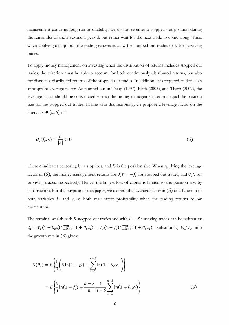
management concerns long-run profitability, we do not re-enter a stopped out position during

the remainder of the investment period, but rather wait for the next trade to come along. Thus,

when applying a stop loss, the trading returns equal for stopped out trades or for surviving

trades.

To apply money management on investing when the distribution of returns includes stopped out

trades, the criterion must be able to account for both continuously distributed returns, but also

for discretely distributed returns of the stopped out trades. In addition, it is required to derive an

appropriate leverage factor. As pointed out in Tharp (1997), Faith (2003), and Tharp (2007), the

leverage factor should be constructed so that the money management returns equal the position

size for the stopped out trades. In line with this reasoning, we propose a leverage factor on the

interval [ ] of:

( ) | |

( )

where indicates censoring by a stop loss, and is the position size. When applying the leverage

factor in ( ), the money management returns are for stopped out trades, and for

surviving trades, respectively. Hence, the largest loss of capital is limited to the position size by

construction. For the purpose of this paper, we express the leverage factor in ( ) as a function of

both variables and , as both may affect profitability when the trading returns follow

momentum.

The terminal wealth with stopped out trades and with surviving trades can be written as:

( ) ∏ ( )

( )

∏ ( ) . Substituting ⁄ into

the growth rate in ( ) gives:

( ) {

( ( ) ∑ ( )

)}

{

( )

∑ ( )

} ( )

9

( ) ( ) [ ( )]∫ ( )

( )

where ( ) denotes the probability of stopped out trades and ( ) denotes the probability

of surviving trades. This growth rate accounts for both the continuously distributed returns of

the surviving trades and for the returns of the stopped out trades. From the growth rate as given

in ( ), we derive a money management criterion that incorporates the stopping of losses for

maximizing the long-run profitability when returns follow momentum.

3.1 The optimal position size and stopping of losses criterion

From the leverage factor in ( ) we may write ( ) ( ). Thus, the investor achieves

long-run profit maximization by maximizing ( ) with respect to both and when stop

loss orders are employed. We assume that ( ) and ( ) are a priori known, and that the investor

achieves ( ) for every on the interval [ ]. By maximizing ( ) with respect to

and , subject to the constraint , we obtain the maximum ( ) at

| |⁄

when ( ) and (

) or at corner solutions ( ), (

). Here,

⁄ and ⁄ . Note that is always a fraction of capital as (

⁄ )

( | | ⁄ ) and, by multiplying throughout with | |, we obtain

. By our

assumptions, we may rule out corner solutions other than ( ), (

) on the interval

studied here.

3.2 The effect of stopping losses on maximum profit

We know from Kaminski and Lo (2013) that the stopping of losses increase profitability if

returns follow momentum, but what is the profitability gain from applying money management

based on an optimal stop distance compared to an arbitrary stop distance?

To answer this question, we now consider the scenario where is exogenous, and where the

investor applies the optimal position size conditional on . By the criterion proposed in this

paper, we may write the profit maximum, conditional on , as ( | ) when (

| ) . We

10

may study the profitability difference using and an arbitrary stop distance, , by comparing

( | ) with (

| ). To study the profitability difference using and any arbitrary , we

consider the maximum profit contour line on the interval [ ], given by:

( ) ( ) ( ( )) [ ( )]∫ (

( )

| | )

( ) ( )

With the stop distance exogenously determined, ( ) is now a function of as it may change

with respect to . Given ( ) , it follows that ( ) for every on the interval [ ].

Further, it follows that ( ) is unique by Theorem 1, and ( ) is a function such that

, on the studied interval. Thus, each point of ( ) represents the maximum profit conditional

on , and the functional form of ( ) reveals how the maximum profit changes with respect to

. Assuming differentiability, we obtain the unconstrained maximum, ( ), when ( ) or

at corner solutions; ( ), ( ).

We study the relative profitability gain by the profit ratio: ( ) ( ) ( )⁄ , where

( ) indicates a relative gain by instead applying optimal stopping of losses, and where

( ) indicates no relative gain.

4. Empirical results

To illustrate the practical relevance of the proposed criterion of this paper, we apply it to a

futures trading strategy together with the Vince criterion. We follow the Rotando and Thorp

(1992) trading strategy where they buy and hold the S&P 500 over one year. The underlying

investment rationale is to profit from a positive price trend. With an annual holding period from

1926 to 1984, we note that their results are based on a total of 59 trades. To study the effects

regarding stopping of losses on profitability, we need more observations of trades to achieve

meaningful results. For this reason we consider a daily analog of the Rotando and Thorp (1992)

strategy, increasing the number of trades considerably, without compromising the underlying

investment rationale. That is, we still expect on average positive daily returns given positive

annual returns. As in the empirical study from Rotando and Thorp (1992), we assume zero costs,

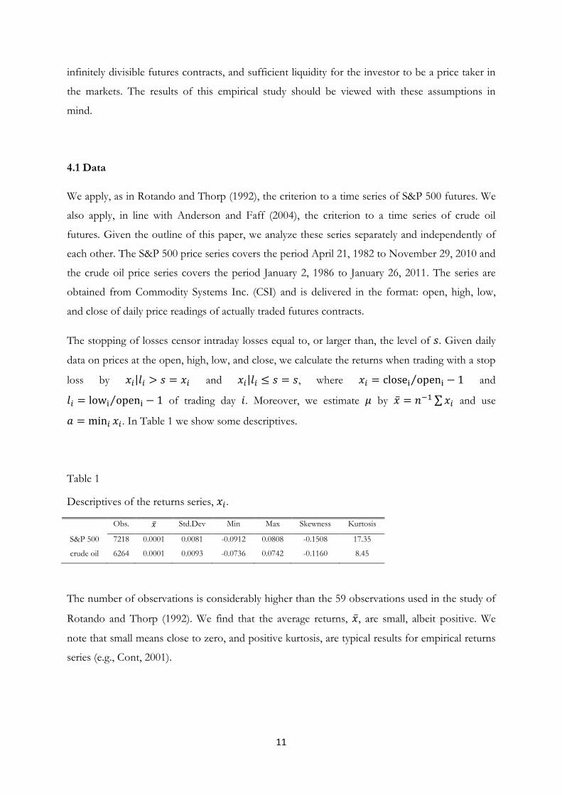
11

infinitely divisible futures contracts, and sufficient liquidity for the investor to be a price taker in

the markets. The results of this empirical study should be viewed with these assumptions in

mind.

4.1 Data

We apply, as in Rotando and Thorp (1992), the criterion to a time series of S&P 500 futures. We

also apply, in line with Anderson and Faff (2004), the criterion to a time series of crude oil

futures. Given the outline of this paper, we analyze these series separately and independently of

each other. The S&P 500 price series covers the period April 21, 1982 to November 29, 2010 and

the crude oil price series covers the period January 2, 1986 to January 26, 2011. The series are

obtained from Commodity Systems Inc. (CSI) and is delivered in the format: open, high, low,

and close of daily price readings of actually traded futures contracts.

The stopping of losses censor intraday losses equal to, or larger than, the level of . Given daily

data on prices at the open, high, low, and close, we calculate the returns when trading with a stop

loss by | and | , where ⁄ and

⁄ of trading day . Moreover, we estimate by ̅ ∑ and use

. In Table 1 we show some descriptives.

Table 1

Descriptives of the returns series, .

Obs. ̅ Std.Dev Min Max Skewness Kurtosis

S&P 500 7218 0.0001 0.0081 -0.0912 0.0808 -0.1508 17.35

crude oil 6264 0.0001 0.0093 -0.0736 0.0742 -0.1160 8.45

The number of observations is considerably higher than the 59 observations used in the study of

Rotando and Thorp (1992). We find that the average returns, ̅, are small, albeit positive. We

note that small means close to zero, and positive kurtosis, are typical results for empirical returns

series (e.g., Cont, 2001).

12

4.2 Numerical approximations

Solving the contour line ( ) in ( ) is non-elementary as is continuously distributed and

cannot be done explicitly. Instead, we estimate ( ) using polynomial regression, which is easy to

apply and estimate, even when the function is non-elementary. The polynomial regression

approximates the functional form, enabling us to study the main dynamics of profitability and to

analytically derive the profit maximum.

To obtain a point on ( ), we first generate a number of values of ( | ) conditional on ,

over the discrete valued domain of { }. We generate values of

( | ) by calculating [ ( ) ∑ ( ) ] conditional on . To

obtain the functional form of ( | ) with respect to , we fit a differentiable, degree

polynomial, ̃( | ), based on the calculated values of ( | ). We find that a step size of

percentage units in is small enough to obtain a concave functional form of ̃ with respect to

. As the polynomial fit is local, we consider only positive values of , ( | ) . We then

analytically solve for the that maximizes ̃. By inserting

into , we obtain a point on ( ).

This procedure is then repeated for each level of in the study.

Second, we estimate ( ) by fitting a differentiable, degree polynomial, ̃( ), based on the

calculated values of ( | ) over the discrete valued domain: { }. To limit the largest

stop distance, we set for both the S&P 500 and crude oil time series. This stop

distance is narrow enough to stop out more than one third of all trades, but still wide enough to

account for temporary large bid ask spreads during volatile market periods, for both assets. We

find that a step size of percentage units in is small enough given this data to obtain a

graphically “smooth” functional form of ( ) with respect to without apparent corners.

Regarding the Vince criterion, we solve for yielding (

) by the same procedure. As the

Kelly and Vince criteria yields identical profitability, we only report the empirical results of the

Vince criterion. We use OLS estimators for the polynomial regressions.

4.3 Results

We estimate ( ) with a third degree polynomial for both assets ( ). For the S&P 500 we

obtain: ̃( ) with and for crude oil

13

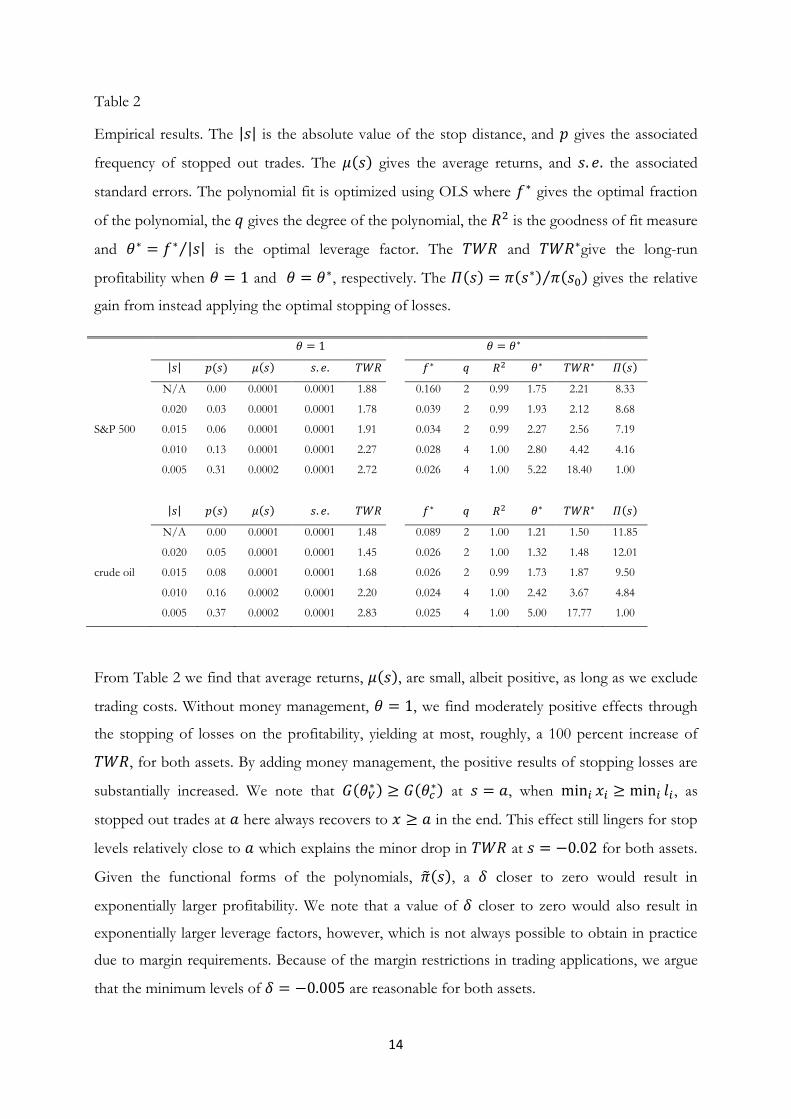
we obtain: ̃( ) with , over the

interval [ ], respectively. Calculations show that the polynomials ̃( ) are exponentially

increasing in , and we find that the profit maxima are corner solutions at , for

both assets. When trading S&P 500, we obtain the profit maximum at ⁄

yielding the , which is 8.33 times the of the Vince criterion. When

trading crude oil, we obtain the profit maximum at ⁄ yielding the

, which is 11.85 times the of the Vince criterion. For smaller than ,

considerable relative gains, ( ), can be made if the investor instead uses the optimal stop

distance. At most this being, 8.68 times, for the S&P 500, and 12.01 times, for the crude oil,

respectively, for .

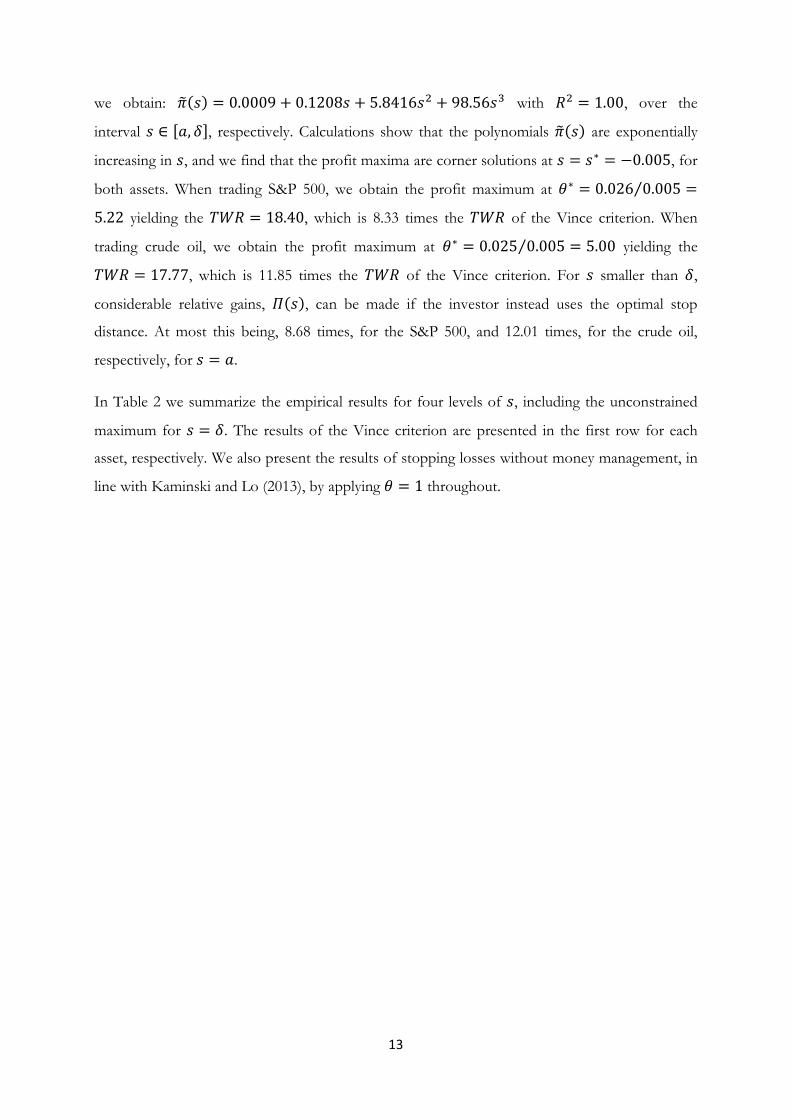
In Table 2 we summarize the empirical results for four levels of , including the unconstrained

maximum for . The results of the Vince criterion are presented in the first row for each

asset, respectively. We also present the results of stopping losses without money management, in

line with Kaminski and Lo (2013), by applying throughout.

14

Table 2

Empirical results. The | | is the absolute value of the stop distance, and gives the associated

frequency of stopped out trades. The ( ) gives the average returns, and the associated

standard errors. The polynomial fit is optimized using OLS where gives the optimal fraction

of the polynomial, the gives the degree of the polynomial, the is the goodness of fit measure

and | |⁄ is the optimal leverage factor. The and give the long-run

profitability when and , respectively. The ( ) ( ) ( )⁄ gives the relative

gain from instead applying the optimal stopping of losses.

| | ( ) ( ) ( )

N/A 0.00 0.0001 0.0001 1.88 0.160 2 0.99 1.75 2.21 8.33

0.020 0.03 0.0001 0.0001 1.78 0.039 2 0.99 1.93 2.12 8.68

S&P 500 0.015 0.06 0.0001 0.0001 1.91 0.034 2 0.99 2.27 2.56 7.19

0.010 0.13 0.0001 0.0001 2.27 0.028 4 1.00 2.80 4.42 4.16

0.005 0.31 0.0002 0.0001 2.72 0.026 4 1.00 5.22 18.40 1.00

| | ( ) ( ) ( )

N/A 0.00 0.0001 0.0001 1.48 0.089 2 1.00 1.21 1.50 11.85

0.020 0.05 0.0001 0.0001 1.45 0.026 2 1.00 1.32 1.48 12.01

crude oil 0.015 0.08 0.0001 0.0001 1.68 0.026 2 0.99 1.73 1.87 9.50

0.010 0.16 0.0002 0.0001 2.20 0.024 4 1.00 2.42 3.67 4.84

0.005 0.37 0.0002 0.0001 2.83 0.025 4 1.00 5.00 17.77 1.00

From Table 2 we find that average returns, ( ), are small, albeit positive, as long as we exclude

trading costs. Without money management, , we find moderately positive effects through

the stopping of losses on the profitability, yielding at most, roughly, a 100 percent increase of

, for both assets. By adding money management, the positive results of stopping losses are

substantially increased. We note that ( ) (

) at , when , as

stopped out trades at here always recovers to in the end. This effect still lingers for stop

levels relatively close to which explains the minor drop in at for both assets.

Given the functional forms of the polynomials, ̃( ), a closer to zero would result in

exponentially larger profitability. We note that a value of closer to zero would also result in

exponentially larger leverage factors, however, which is not always possible to obtain in practice

due to margin requirements. Because of the margin restrictions in trading applications, we argue

that the minimum levels of are reasonable for both assets.

15

If we were to relax the assumption of sufficient liquidity, possible price jumps in the contracts

will consume some of the profits relative to the existing criteria if the stop loss orders are not

executed at the predetermined level (see the discussions of price jumps in Mandelbrot, 1963;

Fama and Blume, 1966). Given the high level of liquidity during US market trading hours for the

assets we study here, price jumps are relatively small. Reasonable estimates are 2 points on

average for both assets. Given an optimal stop level of , price jumps would then, on

average, delay the position exit to for stopped out trades. A priori aware of the

price jump distribution, the investor adjusts the optimal fraction correspondingly. From the

polynomials, ̃( ), we obtain a reduced profitability of when trading the S&P

500 and when trading crude oil.

5. Concluding discussion

This paper proposes the first money management criterion to incorporate optimal stopping of

losses in futures trading. The main contribution is that we may increase the profitability of

trading relative to the existing money management criteria when returns follow momentum. To

illustrate the practical relevance of the proposed criterion of this paper, we apply it to a strategy

of trading S&P 500 and crude oil futures, together with the Vince criterion. Without money

management, we find moderately positive effects on the profitability by stopping losses, yielding

at most, roughly a 100 percent increase of terminal wealth, for both assets. By adding money

management, the positive results of stopping losses are substantially increased. We are able to

improve the empirical profitability 8.33 times the Vince criterion, when trading the S&P 500, and

11.85 times the Vince criterion, when trading crude oil.

The empirical profitability should not be interpreted as the results of actual futures trading as we

exclude all costs associated with trading such as commissions, taxes, and bid ask spreads. In this

paper we focus, however, on the relative profitability between the criterion of this paper and the

existing criteria. We note that the stopping of losses without re-entry does not induce additional

trading costs, and the profitability difference between the criterion of this paper and the Kelly

and Vince criteria remains unchanged, even if costs were included. Admittedly, possible price

jumps will consume some of the profits relative to the existing criteria if the stop loss orders are

not executed at the predetermined level. Although reduced, there remain considerable levels of

profitability relative to the existing criteria, for both assets.

16

The results of this paper are, not surprisingly, driven by relatively few influential trades. This is

natural in investing as the relative profitability from stopping losses comes from prematurely

stopping out a relatively few, large, losses for any trading strategy returns series with positive

kurtosis. As large losses are essentially unpredictable, they are also essentially unavoidable. Thus,

the stopping of losses is well motivated in futures trading even if the results depend on a

relatively few trades. We conclude that money management in futures trading should incorporate

stopping of losses when returns follow momentum.

References

Anderson, J. A. and Faff, R. W. (2004): “Maximizing futures returns using fixed fraction asset

allocation.” Applied Financial Economics, 14, 1067–1073.

Balsara, N. J. (1992): Money Management Strategies for Futures Traders, Wiley Finance, Wiley, New

York.

Basu, D., R. Oomen, and A. Stremme (2010): “How to Time the Commodity Market”, Journal of

Derivatives & Hedge Funds, 1, 1-8.

Biasis, B., P. Hillion, and C. Spatt (1995): “An Empirical Analysis of the Limit Order Book and

the Order Flow in the Paris Bourse”, Journal of Finance, 50, 1655-1689.

Bodie, Z. (1983): “Commodity Futures as a Hedge Against Inflation.” Journal of Portfolio

Management, Spring, 12-17.

Bodie, Z., and V. Rosansky (1980): “Risk and Returns in Commodity Futures.” Financial Analysts

Journal, May/June, 27-39.

Chan, K., A. Hameed, and W. Tong (2000): “Profitability of Momentum Strategies in the

International Equity Markets.” The Journal of Financial and Quantitative Analysis, 35, 153-172.

Chakravarty, S., and C. Holden (1995): “An Integrated Model of Market and Limit Orders”,

Journal of Financial Intermediation, 4, 213-241.

17

Conrad, J., and G. Kaul (1998): “An Anatomy of Trading Strategies”, Review of Financial Studies,

11, 489-519.

Cont, R. (2001): “Empirical properties of asset returns: stylized facts and statistical issues.“

Quantitative Finance, 1, 223-236.

Easley, D., and M. O´Hara (1991): “Order Form and Information in Securities Markets”, Journal

of Finance, 46, 905-927.

Erb, C., and C. Harvey (2006): “The strategic and tactical value of commodity futures”, Financial

Analysts Journal, 62, 69-97.

Faith, C. (2003): The Original Turtle Trading Rules, www.originalturtles.org 2014-04-10.

Fama, E. and M. Blume (1966): “Filter Rules and Stock Market Trading Profits," Journal of

Business, 39, 226-241.

Fuertes, A.M., J. Miffre and G. Rallis (2010): “Tactical Allocation in Commodity Futures

Markets: Combining Momentum and Term Structure Signals," Journal of Banking & Finance, 34,

2530-2548.

Gehm, F. (1983): Commodity Market Money Management, Wiley, New York.

Greer, R.J. (1978): “Conservative Commodities: A Key Inflation Hedge”, Journal of Portfolio

Management, Summer, 26-29.

Handa, P., and R. Schwartz (1996): “Limit Order Trading”, Journal of Finance, 51, 1835-1861.

Harris, L. and J. Hasbrouck (1996): “Market vs. Limit Orders: The SuperDot Evidence on Order

Submission Strategy”, Journal of Financial and Quantitative Analysis, 31, 213-231.

18

Holmberg, U., C. Lonnbark, and C. Lundstrom (2013): ”Assessing the Profitability of Intraday

Opening Range Breakout Strategies,” Finance Research Letters, 10, 27-33.

Jegadeesh, N. and S. Titman (1993): “Returns to Buying Winners and Selling Losers: Implications

for Stock Market Efficiency," Journal of Finance, 48, 65-91.

Jensen, G., R. Johnson, and J. Mercer (2000): “Efficient Use of Commodity Futures in

Diversified Portfolios.” Journal of Futures Markets, 20, 489-506.

Jensen, G., R. Johnson, and J. Mercer (2002): “Tactical Asset Allocation and Commodity

Futures.” Journal of Portfolio Management, Summer, 100-111.

Kaminski, K., and A. Lo (2013): "When Do Stop-Loss Rules Stop Losses?," Journal of Financial

Markets, Article in press.

Katz, J.O., and D.L. McCormick (2000): The Encyclopedia of Trading Strategies, McGraw-Hill, New

York.

Kelly, Jr, J. L. (1956): “A new interpretation of information rate,” The Bell System Technical Journal,

35, 917–926.

Lo, A., C. MacKinlay, and J. Zhang (2002): “Econometric Models of Limit-Order Executions”,

Journal of Financial Economics, 65, 31-71.

Lundström, C. (2013): ”Day Trading Profitability across Volatility States: Evidence of Intraday

Momentum and Mean-Reversion,” Umeå Economic Studies, 861. Umeå University.

MacLean, L. C., E.O. Thorp, and W.T. Ziemba (2010): The Kelly Capital Growth Investment Criterion:

Theory and Practice, Vol. 3 of World Scientific Handbook in Financial Economic Series, World

Scientific, Singapore.

Mandelbrot, B. (1963): “The Variation of Certain Speculative Prices.” The Journal of Business 36,

394–419.

19

Miffre, J. and G. Rallis (2007): “Momentum Strategies in Commodity Futures Markets," Journal of

Banking & Finance, 31, 1863-1886.

Poundstone, W. (2005): Fortune’s Formula: The Untold Story of the Scientific Betting System that Beat the

Casinos and Wall Street, Hill and Wang, New York.

Rotando, L. M. and E.O. Thorp (1992): “The Kelly criterion and the stock market,” The American

Mathematical Monthly, 99, 922–931.

Seppi, D. (1997): “Liquidity Provision with Limit Order and a Strategic Specialist”, Review of

Financial Studies, 10, 103-150.

Sewell, M. (2011): “Money Management.” Research note RN/11/05. The Department of Computer

Science. London University.

Shyy, G. (1989): “Gambler´s ruin and optimal stop loss strategy.” Journal of Futures Markets, 9,

565-571.

Shefrin, M., and M. Statman (1985): “The Disposition to Sell Winners Too Early and Ride Losers

Too Long: Theory and Evidence”, Journal of Finance, 40, 777-790.

Tharp, Van K. (1997): Special Report on Money Management. I.I.T.M., Inc. USA.

Tharp, Van K. (2007): Trade Your Way to Financial Freedom. McGraw-Hill. USA.

Thorp, E.O. (1969): “Optimal gambling systems for favorable games” Review of the International

Statistical Institute, 37, 273–293.

Thorp, E.O. (1997): “The Kelly criterion in blackjack, sports betting, and the stock market,”

Paper presented at: The 10th International Conference on Gambling and Risk Taking Montreal,

June 1997. Published in “Finding the Edge: Mathematical Analysis of Casino Games” (2000), eds

O. Vancura, J. A. Cornelius and W. R. Eadington, Institute for the Study of Gambling and

Commercial Gaming, Reno, 163–213.

20

Tschoegl, A. (1988): “The Source and Consequences of Stop Orders: A Conjecture”, Managerial

and Decision Economics, 9, 83-85.

Vince, R. (1990): Portfolio Management Formulas: Mathematical Trading Methods for the Futures, Options,

and Stock Markets, Wiley, New York.

Vince, R. (1992): The Mathematics of Money Management: Risk Analysis Techniques for Traders, Wiley,

New York.

Vince, R. (1995): The New Money Management: A Framework for Asset Allocation, Wiley, New York.

Vince, R. (2007): The Handbook of Portfolio Mathematics: Formulas for Optimal Allocation & Leverage,

Wiley, Hoboken, New Jersey.

Vince, R. (2009): The Leverage Space Trading Model: Reconciling Portfolio Management Strategies and

Economic Theory, Wiley Trading, Wiley, Hoboken, New Jersey.

Vince, R. (2011): “Optimal f and the Kelly Criterion”, IFTA Journal, 11, 21–28.

Wang, C., and M. Yu (2004): “Trading Activity and Price Reversals in Futures Markets.” Journal of

Banking and Finance, 28, 1337-1361.

Williams, L. (1999): Long-Term Secrets to Short-Term Trading, John Wiley & Sons, Inc., Hoboken,

New Jersey.

Ziemba, R. E. S. and W.T. Ziemba (2007): Scenarios for Risk Management and Global Investment

Strategies, Wiley Finance Series, Wiley, Chichester.

Ziemba, W.T. (2005): “The symmetric downside-risk sharpe ratio”, Journal of Portfolio Management,

32, 108-122.