Monetary Policy,Global Liquidity andCommodity Price Dynamics

#167

RUHR

Ansgar BelkeIngo G. BordonTorben W. Hendricks

ECONOMIC PAPERS

Imprint

Ruhr Economic Papers

Published by

Ruhr-Universität Bochum (RUB), Department of EconomicsUniversitätsstr. 150, 44801 Bochum, Germany

Technische Universität Dortmund, Department of Economic and Social SciencesVogelpothsweg 87, 44227 Dortmund, Germany

Universität Duisburg-Essen, Department of EconomicsUniversitätsstr. 12, 45117 Essen, Germany

Rheinisch-Westfälisches Institut für Wirtschaftsforschung (RWI)Hohenzollernstr. 1-3, 45128 Essen, Germany

Editors

Prof. Dr. Thomas K. BauerRUB, Department of Economics, Empirical EconomicsPhone: +49 (0) 234/3 22 83 41, e-mail: thomas.bauer@rub.de

Prof. Dr. Wolfgang LeiningerTechnische Universität Dortmund, Department of Economic and Social SciencesEconomics – MicroeconomicsPhone: +49 (0) 231/7 55-3297, email: W.Leininger@wiso.uni-dortmund.de

Prof. Dr. Volker ClausenUniversity of Duisburg-Essen, Department of EconomicsInternational EconomicsPhone: +49 (0) 201/1 83-3655, e-mail: vclausen@vwl.uni-due.de

Prof. Dr. Christoph M. SchmidtRWI, Phone: +49 (0) 201/81 49-227, e-mail: christoph.schmidt@rwi-essen.de

Editorial Offi ce

Joachim SchmidtRWI, Phone: +49 (0) 201/81 49-292, e-mail: joachim.schmidt@rwi-essen.de

Ruhr Economic Papers #167

Responsible Editor: Volker Clausen

All rights reserved. Bochum, Dortmund, Duisburg, Essen, Germany, 2010

ISSN 1864-4872 (online) – ISBN 978-3-86788-187-6

The working papers published in the Series constitute work in progress circulated to stimulate discussion and critical comments. Views expressed represent exclusively the authors’ own opinions and do not necessarily refl ect those of the editors.

Ruhr Economic Papers #167

Ansgar Belke, Ingo G. Bordon, and Torben W. Hendricks

Monetary Policy, Global Liquidity and Commodity Price Dynamics

Ruhr Economic Papers #124Bibliografi sche Informationen der Deutschen Nationalbibliothek

Die Deutsche Bibliothek verzeichnet diese Publikation in der deutschen National bibliografi e; detaillierte bibliografi sche Daten sind im Internet über: http//dnb.ddb.de abrufbar.

ISSN 1864-4872 (online)ISBN 978-3-86788-187-6

Ansgar Belke, Ingo G. Bordon, and Torben W. Hendricks1

Monetary Policy, Global Liquidity and Commodity Price Dynamics

AbstractThis paper examines the interactions between money, interest rates, goods and com-modity prices at a global level. For this purpose, we aggregate data for major OECD countries and follow the Johansen/Juselius cointegrated VAR approach. Our empirical model supports the view that, when controlling for interest rate changes and thus dif-ferent monetary policy stances, money (defi ned as a global liquidity aggregate) is still a key factor to determine the long-run homogeneity of commodity prices and goods prices movements. The cointegrated VAR model fi ts with the data for the analysed period from the 1970s until 2008 very well. Our empirical results appear to be overall robust since they pass inter alia a series of recursive tests and are stable for varying compositions of the commodity indices. The empirical evidence is in line with theoreti-cal considerations. The inclusion of commodity prices helps to identify a signifi cant monetary transmission process from global liquidity to other macro variables such as goods prices. We fi nd further support of the conjecture that monetary aggregates convey useful information about variables such as commodity prices which matter for aggregate demand and thus infl ation. Given this clear empirical pattern it appears justifi ed to argue that global liquidity merits attention in the same way as the world-wide level of interest rates received in the recent debate about the world savings and liquidity glut as one of the main drivers of the current fi nancial crisis, if not possibly more.

JEL Classifi cation: E31, E52, C32, F42

Keywords: Commodity prices; cointegration; CVAR analysis; global liquidity; infl ation; international spillovers

February 2010

1 Ansgar Belke, University of Duisburg-Essen and IZA Bonn; Ingo G. Bordon and Torben W. Hendricks, University of Duisburg-Essen. – All correspondence to Ansgar Belke, University of Duisburg-Essen, Universitätsstr. 12, 45117 Essen, Germany, e-mail: ansgar.belke@uni-due.de.

4

1. Introduction

Against the background of steadily increasing global liquidity since the beginning of the

century in most industrial countries as well as in numerous emerging market economies

with a dollar peg, especially China, broad money growth has been running well ahead

of nominal GDP. Surprisingly enough, for a long time, consumer price inflation has

remained largely unaffected by the strong monetary dynamics in many regions in the

world. Over the same time period, however, many countries have experienced sharp but

sequential booms in asset prices, such as commodity, real estate or share prices.1

In the period from 2001 to mid 2008, for instance, house prices increased by 40 to 60

percent in a number of OECD countries, the CRB commodity price index surged by 105

percent in the same period, and also stock prices more than doubled in nearly all major

markets from 2003 to 2008. A similar evolution can be found for oil prices. The oil

price was still low in 2001, but the next six years saw a steady increase that tripled the

price by the middle of 2007. Subsequently, oil prices continued to rise sharply reaching

an all-time high on July 3, 2008, only to be followed by an even more spectacular price

collapse.2 Around the turn-of-year 2008-09, the oil price started to rebound and has now

reached values of around $75 which is about twice as much as at the beginning of 2009.

Many observers feel that the sequential increase of asset prices is the result of liquidity

spillovers to certain asset markets.3

From a monetary policy perspective, the different price dynamics of assets and goods

prices in recent years raises the question as to whether the money-inflation nexus has

been changed (thereby calling into question the close long-term relationship between

monetary and goods price developments that was observed in the past) or whether ef-

fects from previous policy actions are still in the pipeline.4 To investigate the relative

importance of these developments, this study tries to establish an empirical link between

1 See Schnabl and Hoffmann (2007). 2 See Hamilton (2008). 3 See Adalid and Detken (2007) and Greiber and Setzer (2007). 4 The main emphasis in these kinds of studies is on globally aggregated variables, which implies that they do not explicitly deal with spillovers of global liquidity to national variables. The main motivation for this way of proceeding is related to recent research according to which inflation appears to be a global phe-nomenon. So far, the relationship between money growth, different categories of asset prices and goods prices has been little studied in an international context. Only recently have a number of authors sug-gested specific interactions of global liquidity with global consumer price and asset price inflation. See Baks and Kramer (1999), Sousa and Zaghini (2006) and Rüffer and Stracca (2006).

5

money, interest rates, asset prices and goods prices. For this purpose, we apply the coin-

tegrated VAR (CVAR) framework and analyse the impact of global liquidity on com-

modity and goods price inflation. While goods prices adjust only slowly to changing

global monetary conditions due to plentiful supply of consumer goods especially from

emerging markets, asset prices such as commodity prices react much faster since the

supply of commodities cannot be easily expanded and new information is relatively fast

incorporated in these auction-based traded markets. Thus disequilibria on these markets

are generally balanced out by price adjustments.

The paper is structured as follows: Section 2 provides an impression of the global pers-

pective of the monetary transmission process. In section 3, we present an overview of

the literature and apply some simple theoretical considerations to illustrate the potential

impacts of monetary policy on commodity prices. Section 4 turns to the technical details

using the CVAR technique on a global scale and reports on the estimation outcomes.

The final section offers conclusions as well as some policy implications of the results.

2. The global perspective of monetary transmission

Both with respect to global inflation and global liquidity performance, available evi-

dence is strong that the global rather than national perspective is more important when

the monetary transmission mechanism has to be identified and interpreted.5 Considering

the development of global liquidity over time, the question is often raised whether and

to what extent global factors are responsible for it.

A few studies investigate this aspect for the G7 countries and conclude that around 50

percent of the variance of a narrow monetary aggregate can be traced to one common

global factor such as the expansionary monetary policy stance of the Bank of Japan dur-

ing the last few years,6 which has been characterized by a significant accumulation of

foreign reserves and by extremely low interest rates – at some time even approaching

zero. By means of carry trades, financial investors took up loans in Japan and invested

5 For instance, Ciccarelli and Mojon (2005) find that deviations of national inflation from global inflation are corrected over time. Similarly, Borio and Filardo (2007) argue that the traditional way of modelling inflation is too country-centred and a global approach is more adequate. 6 See Rüffer and Stracca (2006).

6

the proceeds in currencies with higher interest rates. This kind of capital transaction has

impacts on the development of monetary aggregates far beyond the special case of Ja-

pan and national borders in general.7

An additional argument in favour of focusing on global instead of national liquidity is

that national monetary aggregates have become more difficult to interpret due to the

huge increase in international capital flows. Simply accounting for the external sources

of money growth and then mechanically correcting for cross-border portfolio flows or

M&A activity, on the presumption of their likely less relevant direct effects on con-

sumer prices, is not a sufficient reaction.8

The concept of global liquidity has attracted growing attention in the empirical literature

in recent years9 and there is empirical evidence of the existence of a global business

cycle.10 D’Agostino and Surico (2009) find that forecasts for US inflation based on

global liquidity are significantly more accurate than those based solely on domestic

data. Some studies have applied VAR or VECM models to data aggregated on a global

level. Important contributions include Rüffer and Stracca (2006), Sousa and Zaghini

(2006) and Giese and Tuxen (2007). These studies discover significant and distinctive

reaction of consumer prices to a global liquidity shock. In contrast, the relationship be-

tween global liquidity and asset prices is mixed. For instance, in the study by Rüffer and

Stracca (2006), a composite real asset price index that incorporates property and equity

prices does not show any significant reaction to a global liquidity shock. Giese and

Tuxen (2007) find no evidence that share prices increase as liquidity expands; however,

they cannot empirically reject cointegrating relationships which imply a positive impact

of global liquidity on house prices.

7 See Schnabl and Hoffmann (2007). 8 Instead, these transactions have to be investigated with respect to their information content and potential wealth effects on residents’ income and on asset prices which might backfire to goods prices as well. See Papademos (2007) and Pepper and Olivier (2006). Giese and Tuxen (2007) stress the fact that in today's linked financial markets shifts in the money supply in one country may be absorbed by demand else-where, but simultaneous shifts in major economies may have significant effects on worldwide asset and goods price inflation. 9 See IMF (2007). 10 See Canova, Ciccarelli, and Ortega (2007).

7

3. Overview of the literature and theoretical considerations

Although the focus of this paper is clearly on the empirical aspect of the subject, we will

address some theoretical issues regarding the linkages between interest rates, money

growth (and thus, liquidity) and asset prices. While there is a vast amount of literature

available on the impact of commodity price developments on the macroeconomy (Cody

and Mills, 1991) and on the role of fundamental factors other than monetary policy for

commodity price developments (Hua, 1998), studies specifically dealing with the im-

pacts of monetary policy on commodity prices are evenly distributed over the last dec-

ades but - especially for countries except the US - still surprisingly scarce.11

Over the last three decades the role of commodity prices in setting monetary policy has

been debated among economists (Angell, 1992). We would like to highlight some im-

portant main strands of this literature which also play a major role in our investigation.

First, one of the main combatants in the field, Jeffrey A. Frankel (1986), has contributed

a kind of overshooting theory of commodity prices. Commodities are exchanged on

fast-moving auction markets and, accordingly, are able to respond instantaneously to

any pressure impacting on these markets. Following a change in monetary policy, their

price reacts more than proportionately, i.e., they overshoot their new long-run equili-

brium, because the prices of other goods are sticky. Other studies checking for the po-

tential theoretical and empirical importance of monetary conditions for the relationship

between commodity prices and consumer goods prices are, for instance, Surrey (1989),

Boughton and Branson (1990, 1991) and Fuhrer and Moore (1992). However, our con-

tribution differs from these papers with respect to the way of modeling and the empiri-

cal methodology.

Furthermore, there is a strand of literature which turns the causality of its research inter-

est on its head and checks for the impact of commodity price developments on the con-

duct of monetary policy. For instance, Bhar and Hamori (2008) empirically investigate

the information content of commodity futures prices for monetary policy. They employ

a cross correlation function approach to empirically analyse the relationship between

11 It has been argued above that commodity prices might represent an early indicator of the current state of the economy because they are usually set in continuous auction markets with efficient information (Cody and Mills, 1991). Hence, some researchers as, for instance, Christiano et al. (1996) act for the inclusion of commodity prices as an explanatory variable in monetary VAR models.

8

commodity futures prices and economic activity as, for instance, consumer prices and

industrial production. They come up with the result that commodity prices can serve as

suitable information variables for monetary policy. This study also clearly supports the

view taken by Bernanke et al. (1997) who take a look at the oil price shocks to analyse

the role of monetary policy in postwar U.S. business cycles. They find that an important

part of the effect of oil price shocks on the economy results not from the change in oil

prices, per se, but from the tighter monetary policy resulting from the change in oil pric-

es. In the same vein, Awokuse and Yang (2003) claim that commodity price indices

serve as important information variables for the conduct of monetary policy because

they represent signals of future movements in macroeconomic variables.

However, there is some doubt that commodity prices can be used effectively in formu-

lating monetary policy because they tend to be subject to large and market-specific

shocks which may not have macroeconomic implications (Marquis and Cunningham,

1990, Cody and Mills, 1991). More importantly in our context and according to a more

monetarist view, other researchers (Bessler, 1984, Pindyck and Rotemberg, 1990, and

Hua, 1998) argue that commodity price movements are at least to some extent the result

of monetary factors and, hence, the causality should run from monetary variables to

commodity prices. However, we would like to argue in this paper that this controversy

can only be settled as a matter of empirical testing.

Some insights into the relationship between money, interest rates, commodity prices and

consumer prices can be derived from the dynamic price adjustment to a liquidity shock

across the commodity sector and the goods market. In the short-term, an expansionary

monetary policy providing the markets with ample liquidity may trigger an immediate

price reaction in the commodity sector, but a more subdued price reaction in the con-

sumer goods market. Over time, however, consumer prices also adjust to the new equi-

librium by proportional changes of the consumer price level. In other words, it is plaus-

ible to argue that in the long term changes in money supply do not lead to any real ef-

fects in money or output. The possibility of different dynamic adjustments of commodi-

ty prices and consumer prices to a monetary shock may also provide an explanation for

the recent shift in relative prices between commodities and consumer goods. In order to

formalise these considerations, we apply the model by Frankel and Hardouvelis (1985)

and begin with a money demand equation as starting point:

9

�� � �� � �� � �� (1),

where �� and �� are the logs of the money supply and the price level, �� represents the

influence of real income, � is the short-term interest rate and � represents the semi-

elasticity of the money demand with respect to the interest rate. The commodities mar-

ket is subject to the arbitrage condition that the expected rate of change of commodity

prices ����� � � ����, minus storage costs ��, is equal to the short-term interest rate:

���� � � ��� � �� � � (2).

The risk premium is assumed to be either zero or contained in the constant storage

costs. For the hypothetical case that commodity and all goods prices in the consumption

basket are perfectly flexible, the relative price of commodities and other goods is conse-

quently invariant with respect to monetary developments. The general price level in this

situation, ��� , is proportional to the price of commodities. Substituting (2) into (1) and

setting ��� equal to ��� results in

�� � ��� � �� � ������ � � ��� � ��� (3).

Solving for ��� gives

��� � � �� �� ��� � ��� � � �

� �� ����� � � ��� (4),

and assuming rational expectations yields

���� � � � �� �� ���� � � �� �� � � �

� �� ����� � � ��� (5).

Substituting (5) into (4), then replace for ���� � and continue recursively results in

��� � � �� ��� � �

� ������� � � �� �� � ����� (6).

10

Therefore, ��� should be viewed as the present discounted sum of the expected future

path of the money supply. Equation (6) could be used directly to interpret the reactions

of commodity prices to monetary developments provided that the hypothesis of perfect-

ly flexible goods prices in the economy is correct and adjusting directly in response to

monetary conditions is given.

Considering the other setting in which the prices of most goods and services are as-

sumed to be sticky in the short run, this equation cannot be used to indicate the reaction

of either the general price level or of commodity prices. Assuming for this situation that

the general price level adjusts only gradually over time and only in the long run moves

with ���, then it can be shown that commodity prices will react in the same direction as

���, but will move more than proportionally in the short run:

���� � �� � ���� ���� (7),

where � represents the fraction of the deviation from long-run equilibrium ��� that �� can

be expected to close each period. Equation (7) was first developed by Dornbusch (1976)

in his famous overshooting model for exchange rate determination. Frankel and Har-

douvelis (1985) adopt this to commodity prices to show how the spot price of commodi-

ties reacts more than proportional to a sudden permanent change in the money supply,

that is, how commodity prices overshoot their long-run equilibrium compensating for

the laggard movement in goods prices.12 In the special case of perfectly flexible adjust-

ment of all prices, � is infinite and (7) reduces to the aforementioned case in which

���� is equal to ����. Combining equations (6) and (7) results in

���� � �� � ���� � �� �

� ��� � �� ��

����� � � �� ���� (8).

In a money supply process with permanent disturbances to the trend and transitory dis-

turbances to the level, Mussa (1975) has shown that this linear form is the rational one

to take for market expectations. As a result, the reaction in commodity prices is linearly

related to monetary conditions. Accordingly, the possibility of different dynamic ad-

justments of price elastic and inelastic goods to a monetary shock may provide an ex- 12 See also Frankel (1986) for the detailed version of the model.

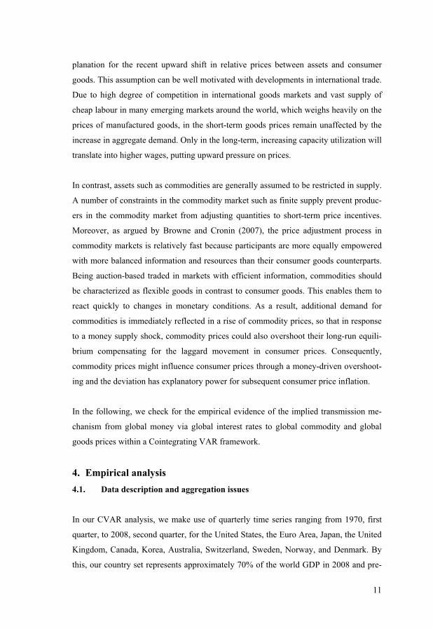
11

planation for the recent upward shift in relative prices between assets and consumer

goods. This assumption can be well motivated with developments in international trade.

Due to high degree of competition in international goods markets and vast supply of

cheap labour in many emerging markets around the world, which weighs heavily on the

prices of manufactured goods, in the short-term goods prices remain unaffected by the

increase in aggregate demand. Only in the long-term, increasing capacity utilization will

translate into higher wages, putting upward pressure on prices.

In contrast, assets such as commodities are generally assumed to be restricted in supply.

A number of constraints in the commodity market such as finite supply prevent produc-

ers in the commodity market from adjusting quantities to short-term price incentives.

Moreover, as argued by Browne and Cronin (2007), the price adjustment process in

commodity markets is relatively fast because participants are more equally empowered

with more balanced information and resources than their consumer goods counterparts.

Being auction-based traded in markets with efficient information, commodities should

be characterized as flexible goods in contrast to consumer goods. This enables them to

react quickly to changes in monetary conditions. As a result, additional demand for

commodities is immediately reflected in a rise of commodity prices, so that in response

to a money supply shock, commodity prices could also overshoot their long-run equili-

brium compensating for the laggard movement in consumer prices. Consequently,

commodity prices might influence consumer prices through a money-driven overshoot-

ing and the deviation has explanatory power for subsequent consumer price inflation.

In the following, we check for the empirical evidence of the implied transmission me-

chanism from global money via global interest rates to global commodity and global

goods prices within a Cointegrating VAR framework.

4. Empirical analysis 4.1. Data description and aggregation issues

In our CVAR analysis, we make use of quarterly time series ranging from 1970, first

quarter, to 2008, second quarter, for the United States, the Euro Area, Japan, the United

Kingdom, Canada, Korea, Australia, Switzerland, Sweden, Norway, and Denmark. By

this, our country set represents approximately 70% of the world GDP in 2008 and pre-

12

sumably a considerably larger share of the global financial markets.13 For the aforemen-

tioned countries, we have collected data for real GDP (Y), the consumer price inflation

(CPI), the three-month Treasury bill rate (TBR) as the short-term interest rate, broad

money aggregates and two commodity price indices. The selected monetary aggregates

are M2 for the U.S. and Japan, M3 for the Euro Area, and mostly M3 or M4 for the oth-

er countries.14 By the method described below, we compute the ratio of global nominal

money to nominal world GDP (LIQ) as global liquidity indicator, a measure commonly

used as a sensor of excess liquidity (see, e.g., Rüffer and Stracca, 2006). The two com-

modity price indices we take into account in our analysis are the Commodity Research

Bureau (CRB) and the CRB Raw Industrials (CRBRI) index. The CRB provides an en-

compassing gauge of price trends in commodity markets because the most important 19

commodities are involved in this index. These markets are presumed to be amongst the

first to be influenced by changes in economic conditions and would, therefore, be ex-

pected to be sensitive to developments in the monetary environment. It consists of ener-

gy (39%), softs/ tropicals (21%), grains/ livestock (20%), and industrial/ precious met-

als (20%). Along with this most broadly defined CRB index, a major division of the

index, the CRBRI index, is used for robustness analysis. It comprises raw industrial

materials/ metals but excludes the volatile food and energy parts.15 An advantage of

using indices of commodity groups rather than individual commodity prices is that idio-

syncratic factors impacting on individual commodity markets should have far less influ-

ence at the level of a multi-commodity, broadly-based index.

We start with aggregating the country-specific time series to produce a global series,

strictly following the guidelines provided by Beyer et al. (2000) and applied by Giese

and Tuxen (2007) in the same context. First, we calculate variable weights for each

country by using PPP exchange rates to convert nominal GDP into a single currency.16

Hence, the weight of country i in period t is given by:

!"#� � $%&'#()'#(***

$%&+,,#( (9).

13 Own calculations based on IMF data. 14 The data are taken from the IMF, the BIS, Thomson Financial Datastream and the EABCN database and are seasonally adjusted where available or treated with the X12-ARIMA procedure. 15 In the following, we present mostly the results for the broad CRB index as the robustness analysis yields comparable outcomes using the CRBRI index instead of the CRB. The results are available upon request by the authors. 16 1999 is our base year for the PPP exchange rates.

13

Secondly, we start with the growth rates of the variable in the domestic currency and

amalgamate them to global growth rates by applying the weights calculated above:

-.//#� � 0 !"#�-"#���"1� 2 (10).

Finally, aggregate levels are then obtained by choosing an initial value of 100 and mul-

tiplying with the computed global growth rates. This gives the level of each variable as

an index:

345678 � 9 2:� � -.//#�;8�1� 2 (11).

This method is applied to all variables except the commodity price indices, which al-

ready represent price developments at a global level and the aggregation for the short-

term interest rate is performed without calculating growth rates. With respect to the

measure of global liquidity, this method lowers the bias resulting from different national

definitions of broad money which obviously exist. Forming a simple sum of national

monetary aggregates – as often conducted in the related literature - would under-

represent countries with narrower definitions of the monetary aggregate and vice versa.

Using this methodology we also avoid the so-called ‘dollar bias,’ which results from

converting national monetary aggregates with actual exchange rates into U.S. dollar and

constructing a simple unweighted sum to obtain global money. For instance, the sharp

fall of the dollar between 1985 and 1988 or the continuous depreciation from 2001 to

2008 would result in an overestimation of global monetary growth.

Figure 1 about here

Figure 1 displays the time path of the globally aggregated time series under investiga-

tion. The CPI series reflects the great inflation of the 1970s until the mid 1980s, fol-

lowed by modest inflation rates afterwards. Even more moderate CPI inflation started to

emerge around the mid 1990s and has persisted until the end of the sample although the

liquidity measure expanded heavily in the last decade. Global short-term interest rates

started to decrease in 1982 and were at historically low levels since 2001 due to the

monetary loosing starting at this time. A closer inspection of the global time series re-

14

veals that in recent years global excess liquidity has been accompanied by strong price

increases in the commodity markets. The ongoing discussion about the linkage of global

excess liquidity and asset price inflation is not at least based on the co-movement in this

period. In the following econometric analysis we will examine this co-movement of

global liquidity and commodity price inflation more deeply.

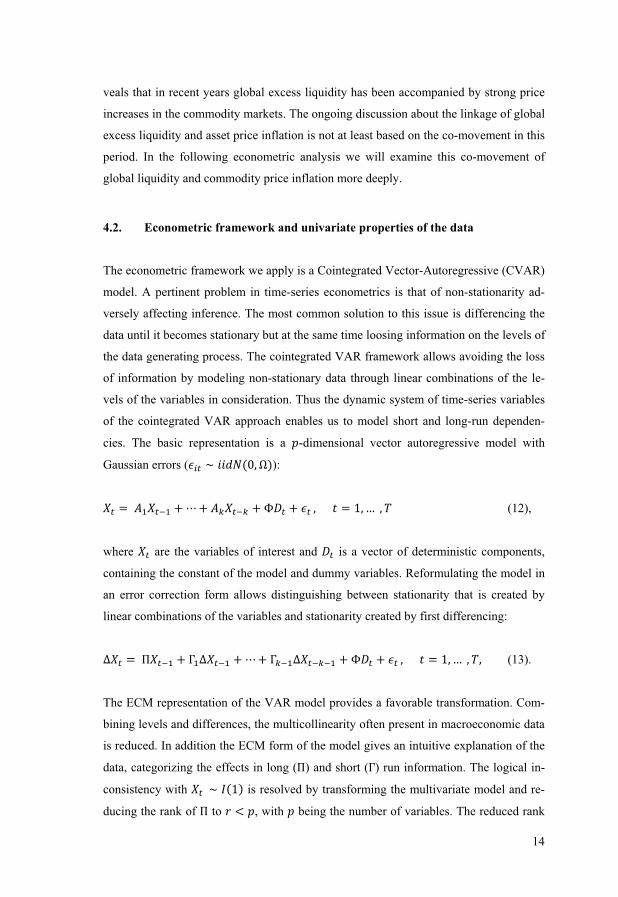
4.2. Econometric framework and univariate properties of the data

The econometric framework we apply is a Cointegrated Vector-Autoregressive (CVAR)

model. A pertinent problem in time-series econometrics is that of non-stationarity ad-

versely affecting inference. The most common solution to this issue is differencing the

data until it becomes stationary but at the same time loosing information on the levels of

the data generating process. The cointegrated VAR framework allows avoiding the loss

of information by modeling non-stationary data through linear combinations of the le-

vels of the variables in consideration. Thus the dynamic system of time-series variables

of the cointegrated VAR approach enables us to model short and long-run dependen-

cies. The basic representation is a �-dimensional vector autoregressive model with

Gaussian errors (<"� = 335>�?# @�):

A� � 2B�A�C� � D� BEA�CE � FG� � <�2#222222H � �#I2# J (12),

where A� are the variables of interest and G� is a vector of deterministic components,

containing the constant of the model and dummy variables. Reformulating the model in

an error correction form allows distinguishing between stationarity that is created by

linear combinations of the variables and stationarity created by first differencing:

KA� � 2LA�C� � M��A�C� � D� MEC��A�CEC� � FG� � <�2#222222H � �#I2# J# (13).

The ECM representation of the VAR model provides a favorable transformation. Com-

bining levels and differences, the multicollinearity often present in macroeconomic data

is reduced. In addition the ECM form of the model gives an intuitive explanation of the

data, categorizing the effects in long (L) and short (M) run information. The logical in-

consistency with A�2 = N��� is resolved by transforming the multivariate model and re-

ducing the rank of L to O �, with � being the number of variables. The reduced rank

15

matrix can be factorised into two � P matrices Q and R (L � STU). The factorization

provides stationary linear combinations of the variables (cointegrating vectors) and

� � common stochastic trends of the system. Formulating the cointegration hypothe-

sis as a reduced rank condition on the matrix L � STU implies that the processes KA�

and RUA� are stationary, while the levels of the variables A� are nonstationary. Therefore

the ECM model allows for the variables contained in A� to be integrated of order 1

(I(1)).

To access the unit root properties of the individual time series used by us we apply

Augmented Dickey-Fuller (ADF) and Phillips-Perron (PP) test statistics to the natural

logs of our variables of consideration, except the interest rate, which is verified in its

level.

Table 1 about here

Table 1 reports that the levels of all series are clearly non-stationary using standard

ADF tests, where the appropriate lag length is selected by the Akaike Information Crite-

rion (AIC) and by the Schwarz Bayesian Criterion (SBC). The Phillips–Perron (PP)

tests corroborate these results. Looking at the results for the first-differences conveys

empirical evidence that most of the series can be assumed to be integrated of order one.

However, the only exception is the CPI data for which the empirical realization of the

test statistics gives mixed results. The PP test clearly indicates that CPI can be consi-

dered as integrated of order 1 (I(1)), an assessment which is confirmed by the ADF test

with respect to the SBC at the 10% significance level. However, the ADF test specified

according to the AIC does not reject the null hypothesis of a unit root. However, Greene

(2008) and Hamilton (1994) observe that the ADF test tends to fail to distinguish be-

tween a unit root and a near unit root process and too often indicates that a series con-

tains a unit root. Furthermore, they argue that the SBC is superior to the AIC in the case

of a large sample. Given these arguments and the fact that we dispose of a sample size

of 154 observations and an empirical realization of the ADF test statistic based on the

AIC only marginally larger than the 90 per cent critical value of -3.146, we feel legiti-

mized to continue assuming that all series are each integrated of order one. We now

proceed with the lag length selection and diagnostic testing on the unrestricted VAR

model.

16

4.3. Lag length selection and diagnostic testing on the unrestricted VAR model

Since all asymptotic results as the choice of the cointegrating rank depend on the appro-

priateness of specification of the underlying model, we now focus on testing the ade-

quacy of the econometric model used by us.

Specifying the lag length of the VAR has strong implications for our subsequent model-

ing choices. Choosing too few lags could lead to systematic variation in the residuals

whereas choosing too many lags comes with the penalty of fewer degrees of freedom

(as adding another lag, adds � P � variables). In macroeconomic modeling it is hard to

imagine agents using information that reaches back much further than two to four quar-

ters. Hence, a lag length of two is generally encouraged. With regards to the formal test-

ing based on the maximum of the likelihood function, the choice of a lag length of two

is supported for our data by the “Schwartz” and “Hannan-Quinn” information criteria.

Estimation of our VAR model is based on the assumption that the residuals display

Gaussian properties. Extraordinarily large shocks corresponding to economic reforms or

intervention and by those possibly marking structural breakpoints in the data series tend

to cause a violation of the normality assumption. The deviation from the normality as-

sumption leads to incorrect statistical inferences. Hence, it is quite important to identify

the dates of such shocks and to correct them with intervention dummies (Juselius,

2006). The global data used here seem overall well behaved. However, our formal resi-

dual analysis suggests the inclusion of dummy variables to deal with potentially non-

Gaussian properties of the residuals.

Table 2 about here

Table 2 reports a univariate and multivariate residual analysis of the unrestricted

VAR(2). Based on these results, the multivariate LM(1) and LM(2) tests reject autocor-

relation in the first and second lag of the residuals. We reject the null of normality for

the multivariate model due to empirical evidence of deviations from normality in skew-

ness and/or kurtosis for the global liquidity and the global interest rate series. Although

the commodity price time series display high fluctuations especially in the last period of

17

the data sample, there is hardly any evidence of 2nd order ARCH effects according to the

univariate statistics. We do not consider even moderate ARCH-effects as highly prob-

lematic since Rahbek et al. (2002) show that the cointegration rank testing is still robust

in this case. Our formal misspecification tests indicate rejection of multivariate normali-

ty and ARCH effects due to the above mentioned features of the global liquidity and

interest rates series. Overall the VAR(2) model seems to provide a reasonable descrip-

tion of the information contained in the data. We now estimate our global CVAR after

having determined its rank.

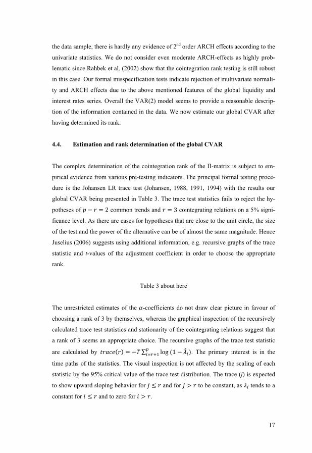
4.4. Estimation and rank determination of the global CVAR

The complex determination of the cointegration rank of the L-matrix is subject to em-

pirical evidence from various pre-testing indicators. The principal formal testing proce-

dure is the Johansen LR trace test (Johansen, 1988, 1991, 1994) with the results our

global CVAR being presented in Table 3. The trace test statistics fails to reject the hy-

potheses of � � � V common trends and � W cointegrating relations on a 5% signi-

ficance level. As there are cases for hypotheses that are close to the unit circle, the size

of the test and the power of the alternative can be of almost the same magnitude. Hence

Juselius (2006) suggests using additional information, e.g. recursive graphs of the trace

statistic and t-values of the adjustment coefficient in order to choose the appropriate

rank.

Table 3 about here

The unrestricted estimates of the Q-coefficients do not draw clear picture in favour of

choosing a rank of 3 by themselves, whereas the graphical inspection of the recursively

calculated trace test statistics and stationarity of the cointegrating relations suggest that

a rank of 3 seems an appropriate choice. The recursive graphs of the trace test statistic

are calculated by HX�6�� � �J � YZ[2�� � �\"�]"1^ � . The primary interest is in the

time paths of the statistics. The visual inspection is not affected by the scaling of each

statistic by the 95% critical value of the trace test distribution. The trace (j) is expected

to show upward sloping behavior for _ ` and for _ a to be constant, as �" tends to a

constant for 3 ` and to zero for 3 a .

18

Figure 2 about here

Figure 2 illustrates the recursive estimated trace statistics. The graphs based on the con-

centrated model R1 render support to our choice of a rank of 3 with 2 linearly growing

trace statistics and the third being a borderline case. As will be pointed out below, in-

cluding the third cointegrating relation is yet favoured by the identification of the long-

run structure and our recursive tests of parameter constancy.

Figure 3 about here

Figure 3 illustrates the long-run disequilibrium error of the first, second and third coin-

tegrating relation. The time paths indicate a fairly stable and stationary pattern support-

ing our choice of a rank of 3.

4.5. Identification of the long-run structure and hypothesis testing of the re-

stricted model

As mentioned in section 4.3., the existence of outliers in the underlying data set leads to

autocorrelation and distortion of the residual distribution. In addition to accounting for a

deterministic trend in the data by specifying the model including a trend term restricted

to the cointegration space, we correct for innovational outliers. More specifically, we

include three permanent impulse dummies taking the value one in the given quarter of

the respective year and zero elsewhere:

G� � bGcd?��# Gce?V�# Ge??d�f�2 (14).

The information set is defined by the variable vector

7�g � bhiN# hjk# lNm# Jkj# nf�2 (15).

Table 4 about here

The restrictions for the long-run specification for r=3 and a lag length of k=2 are not

rejected with a p-value of 0.309 (o�(1) = 1.034) and the results are presented in Table 4.

19

R\�gp2hjk � hiN � Wq?rs2b�tq?c�flNm � dqd�t2bsq�e�fJjk � ?q??c2bcqsccfH = N�?�

(16)

R\�g p Jjk � ?qV?t2bdqs�sfn � ?qWWc2b��VqrctfhiN � ?qV?d2b�?qtc�fhjk = N�?�

(17)

R\ug p hjk � dq?rc2b�rqtssflNm � ?q?ee2b�?qs?dfhiN = N�?� (18)

The empirically identified long-run structure represented by the cointegrating relations

R\�g , R\�g and R\ug is guided by economic reasoning. The first cointegrating relation

represents the price spread of commodities and consumer goods with the former being

characterized as the flexibly adjusting quantity. The deviation of commodity prices from

consumer prices is significantly driven by excess liquidity and is negatively related with

the interest rate. R\�g can be interpreted as a Taylor-rule-type relation where the interest

rate is positively connected to inflation. Given that the interest rate is inversely reacting

to output and commodity prices it seems more appropriate to read the second long-run

relation in a sense as a “failing” Taylor-rule-type relation, as the interest rate does not

seem to have been adjusted enough in the long-run to account for commodity price in-

flation and output growth on a global scale. The third long-run relation again conveys

empirical evidence of commodity prices positively reacting to global liquidity and con-

sumer price inflation, whereas the latter goes without statistically significance.

Figures 4 and 5 about here

We corroborate the appropriateness of the model in describing the long-run properties

of the data by means of the recursively calculated test of beta-constancy and the log-

likelihood constancy depicted in Figure 4 and 5. The time path of the tests indicate that

overall the model performs well. Apart from identifying the long-run equilibriums, the

understanding of the system’s structure is enhanced by analyzing the Q-vectors. Testing

for a zero row of the commodity price variable in the Q-matrix corresponding to the

identified long-run structure is accepted with a p-value of 0.351 (o�(4) = 4.426). Thus

the commodity prices do not display error-correcting behavior to the cointegrating rela-

tions pointing to a dynamic of the commodity prices that potentially compensates the

rather sluggish adjustment of consumer prices. The latter can be characterized as com-

20

pletely endogenous, as the respective test of the corresponding2Q-vectors is rejected

with a p-value of 0.000 (o�(4) = 45.910).

Our empirical analysis is broadly supportive of the model and the theoretical hypothes-

es. The impression of a long-run proportional relationship between global money and

prices has been hardened by our cointegration analysis. The cointegration error-terms

have explanatory power for ensuing consumer price inflation. The deviation of com-

modity prices from their long-run equilibrium explains subsequent consumer price in-

flation. By establishing the monetary driven commodity price development within the

cointegration analysis framework, we have gained support for deducing that the feed-

back from commodity prices to consumer prices is a monetary phenomenon.

5. Conclusions and policy implications

The main empirical results of our paper are the following: At a global level, we find

further support of the conjecture that monetary aggregates may convey some useful in-

formation on variables such as commodity prices which matter for aggregate demand

and hence inflation. Moreover, we identify a negative relation between the world inter-

est rate and commodity prices as proposed by Frankel and Hardouvelis (1985). Thus,

we conclude that global liquidity and the world interest rate are useful indicators of

commodity price inflation and of a more generally defined inflationary pressure at a

global level.

As a by-product, we are able to identify a Taylor-rule-type relation where the interest

rate is positively connected to inflation. Given that the interest rate is inversely reacting

to output and commodity prices, it seems more appropriate to read the second long-run

relation in a sense as a failing Taylor-rule-type relation, as the interest rate doesn’t seem

to have been adjusted enough in the long-run to account for commodity price inflation

and output growth on a global scale.

Therefore we would like to argue that global liquidity merits some attention in the same

way as the worldwide level of interest rates received in the recent hot debate about the

world savings and liquidity glut as the main drivers of the current financial crisis, if not

possibly more.

21

Expressed on a more technical level, this paper has analysed the relationship among

money, interest rates and commodity prices on a global scale. At the OECD level, we

find further support of the conjecture that monetary aggregates may convey some useful

information about the future development of commodity prices which matter for aggre-

gate demand and hence consumer price inflation. Our empirical results appear to be

overall robust since they pass inter alia a series of recursive tests and are stable for vary-

ing compositions of the commodity indices.

Our findings do also provide some support for considering commodity price indices

along with other information variables as early indicators of more general inflation and,

by this, emphasize rather early claims by Furlong (1989) and Garner (1985).17 One fur-

ther advantage might be the more timely availability of commodity price data relative to

those on overall prices. Thus, we conclude that liquidity is a useful indicator of com-

modity price inflation.

Against this background, a high level of global liquidity can generally be seen as a

threat to future asset price inflation and financial stability.18 Since global liquidity is

found to be an important determinant of commodity prices and there is long-run homo-

geneity among commodity and goods prices, there might be at least one implication.

Monetary authorities have to be aware of likely spill-overs from commodity to consum-

er prices. We also see some implications for policy makers emanating from our empiri-

cal results. In the first place, our CVAR analysis indicates that commodity prices might

well serve as indicators of future more general inflationary pressures. Moreover, strong

monetary growth might be a good indicator of emerging bubbles in the commodity sec-

tor. Hence, asset price movements should certainly play a role in policy.

17 Bhar and Hamori (2008) and Furlong and Ingenito (1996) focus less on the role of monetary policy in a relationship like presented in our CVAR and more on the signaling or predictive power of commodity prices for consumer price inflation. Accordingly, Sims (1998) and Sims and Zha (1998) emphasize the importance of introducing the commodity price variable in designing monetary policy rules. 18 See the early and continuous publics about the latter by the ECB Observer group as expressed, for in-stance, in Belke et al. (2004). For details see http://www.ecb-observer.com.

22

References

Adalid, R., Detken, C., 2007. Liquidity Shocks and Asset Price Boom/Bust Cycles. ECB Working Paper Series 732, Frankfurt a. M.

Angell, W. D., 1992. Commodity Prices and Monetary Policy: What Have We Learned? Cato Journal 12, 185-192.

Awokuse, T. O., Yang, J., 2003. The Information Role of Commodity Prices in Formu-lating Monetary Policy: A Re-examination. Economics Letters 79, 219–224.

Baks, K., Kramer, C. F., 1999. Global Liquidity and Asset Prices: Measurement, Impli-cations and Spillovers. IMF Working Papers 99/168, Washington, D. C.

Belke, A., Kösters, W., Leschke, M., Polleit, T., 2004. Towards a “More Neutral” Monetary Policy. ECB Observer No. 7, Frankfurt a. M.

Bernanke, B. S., Gertler, M., Watson, M., Sims, C. A., Friedman, B. M., 1997. Symme-tric Monetary Policy and the Effects of Oil Price Shocks. Brookings Papers on Economic Activity 1, 91–174.

Bessler, D. A., 1984. Relative Prices and Money: A Vector Autoregression on Brazilian Data. American Journal of Agricultural Economics 66, 25–30.

Beyer, A., Doornik, J. A., Hendry, D. F., 2000. Constructing Historical Euro-Zone Data. Economic Journal 111, 308-327.

Bhar, R., Hamori, S., 2008. Information Content of Commodity Futures Prices for Monetary Policy. Economic Modelling 25, 274–283.

Borio, C. E. V., Filardo, A., 2007. Globalisation and Inflation: New Cross-Country Evi-dence on the Global Determinants of Domestic Inflation. BIS Working Papers 227, Basle.

Boughton, J. M., Branson, W. H., 1990. The Use of Commodity Prices to Forecast In-flation. Staff Studies for the World Economic Outlook, IMF, 1-18.

Boughton, J. M., Branson, W. H., 1991. Commodity Prices as a Leading Indicator of Inflation. In Lahiri, K., Moore, G. H., (eds.), Leading Economic Indicators – New Approaches and Forecasting Records, Cambridge University Press, 305-338.

Browne, F., Cronin, D., 2007. Commodity Prices, Money and Inflation. ECB Working Paper 738, Frankfurt a. M.

Canova, F., Ciccarelli, M., Ortega, E., 2007. Similarities and Convergence in G-7 Cy-cles, Journal of Monetary Economics 54, 850-878.

Christiano, L. J., Eichenbaum, M., Evans, C., 1996. The Effects of Monetary Policy Shocks: Evidence from the Flow of Funds. Review of Economics and Statistics 78, 16–34.

Ciccarelli, M., Mojon, B., 2005. Global Inflation. ECB Working Paper Series 537, Frankfurt a. M.

Cody, B. J., Mills, L. O., 1991. The Role of Commodity Prices in Formulating Mone-tary Policy. Review of Economics and Statistics 73, 358–365.

D’Agostino, A., Surico, P., 2009. Does Global Liquidity Help to Forecast U.S. Infla-tion? Journal of Money, Credit and Banking 41, 479-489.

Dornbusch, R., 1976. Expectations and Exchange Rate Dynamics. Journal of Political Economy 84(6), 1161-1176.

23

Frankel, J. A., 1986. Expectations and Commodity Price Dynamics: The Overshooting Model. American Journal of Agricultural Economics 68(2), 344-348.

Frankel, J. A., Hardouvelis, G. A., 1985. Commodity Prices, Money Surprises and Fed Credibility. Journal of Money, Credit and Banking 17(4), 425-438.

Fuhrer, J., Moore, G., 1992. Monetary policy rules and the indicator properties of asset prices. Journal of Monetary Economics, 29(2), 303-336.

Furlong, F. T., 1989. Commodity Prices as a Guide for Monetary Policy. Economic Review Federal Reserve Bank of San Francisco 1, 21-38.

Furlong, F., and Ingenito, R., 1996. Commodity Prices and Inflation. Economic Review Federal Reserve Bank of San Francisco 2, 27-47.

Garner, C. A., 1985. Commodity Prices and Monetary Policy Reform. Economic Re-view Federal Reserve Bank of Kansas City, 7-21.

Giese, J. V., Tuxen, C. K., 2007. Global Liquidity and Asset Prices in a Cointegrated VAR. Nuffield College, University of Oxford, and Department of Economics, Copenhagen University.

Greene, W., 2008. Econometric Analysis. 6th Edition, Prentice-Hall.

Greiber, C., Setzer, R., 2007. Money and Housing: Evidence for the Euro Area and the US. Deutsche Bundesbank Discussion Paper Series: Economic Studies 07/12, Frankfurt a. M.

Hamilton, J. D., 1994. Time Series Analysis, Princeton University Press, Princeton, NJ.

Hamilton, J.D., 2008. Understanding Crude Oil Prices, Department of Economics, Uni-versity of California, San Diego, December 6.

Hua, P., 1998. On Primary Commodity Prices: The Impact of Macroeconomic and Monetary Shocks. Journal of Policy Modeling 20, 767-790.

IMF, 2007. What is Global Liquidity? World Economic Outlook Globalization and Ine-quality, Chapter I, October, Washington, D.C.

Johansen, S., 1988. Statistical Analysis of Cointegrated Vectors. Journal of Economic Dynamics and Control 12(3), 231-54.

Johansen, S., 1991. Estimation and Hypothesis Testing of Cointegrated Vectors in Gaussian Vector Autoregressive Models. Econometrica 59(6), 1551-1580.

Johansen, S., 1994. The Role of the Constant and Linear Terms in Cointegration Analy-sis of Nonstationary Variables. Econometric Review 13(2), 205-229.

Juselius, K., 2006. The Cointegrated VAR Model: Econometric Methodology and Mac-roeconomic Applications, Oxford University Press.

Marquis, M. H., Cunningham, S. R., 1990. Is There a Role of Commodity Prices in the Design of Monetary Policy? Some Empirical Evidence. Southern Economic Jour-nal 57, 394–412.

Mussa, M. (1975). Adaptive and Regressive Expectations in a Rational Model of the Inflationary Process. Journal of Monetary Economics, 1(4), 423-442.

Papademos, L., 2007. The Effects of Globalisation on Inflation, Liquidity and Monetary Policy. Speech at the conference on the ”International Dimensions of Monetary Policy” organised by the National Bureau of Economic Research, S’Agar`o, Gi-rona, June 11th 2007.

24

Pepper, G., Olivier, M., 2006. The Liquidity Theory of Asset Prices. Wiley Finance.

Pindyck, R. S., Rotemberg, J. J., 1990. The Excess Co-movement of Commodity Prices. Economic Journal 100, 1173–1189.

Rahbek, A., Hansen E., Dennis J. G., 2002. ARCH Innovations and their Impact on Cointegration Rank Testing, Department of Theoretical Statistics, Centre for Ana-lytical Finance, University of Copenhagen, Working Paper no.22.

Rüffer, R., Stracca, L., 2006. What Is Global Excess Liquidity, and Does It Matter? ECB Working Paper Series 696, Frankfurt a. M.

Schnabl, G., Hoffmann, A., 2007. Monetary Policy, Vagabonding Liquidity and Burst-ing Bubbles in New and Emerging Markets – An Overinvestment View. CESifo Working Paper 2100, Munich.

Sims, C., 1998. The role of interest rate policy in the generation and propagation of business cycles: What has changed since the 30's?. In: Fuhrer, J. C., Schuh, S. (Eds.), Beyond Shocks: What Causes Business Cycles? Federal Reserve Bank of Boston Conference Series 42.

Sims, C., Zha, T., 1998. Does Monetary Policy Generate Recessions? Federal Reserve Bank of Atlanta Working Paper, 98-12.

Sousa, J. M., Zaghini, A., 2006. Global Monetary Policy Shocks in the G5: A SVAR Approach. CFS Working Paper Series 2006/30, Frankfurt a. M.

Surrey, M. J. C., 1989. Money, Commodity Prices and Inflation: Some Simple Tests. Oxford Bulletin of Economics and Statistics 51(3), 219-238.

25

Figure 1: Time path of the aggregated global series from 1970:01 to 2008:02 (in logs, except for the interest rate)

Figure 2: Recursively calculated trace test statistics based on the full and the concentrated model (Base sample 1970:04 to 1978:1)

1970 1975 1980 1985 1990 1995 2000 2005

5.0

5.5Y

1970 1975 1980 1985 1990 1995 2000 2005

5.0

5.5

6.0

6.5CPI

1970 1975 1980 1985 1990 1995 2000 2005

5.0

5.5

6.0CRB

1970 1975 1980 1985 1990 1995 2000 2005

5

10TBR

1970 1975 1980 1985 1990 1995 2000 2005

4.8

5.0LIQ

26

Figure 3: The cointegrating relations vwx

� yxz, vw{� yxz and vw|

� yxz

Figure 4: Recursively calculated max test of v constancy (Base sample 1970:04 to 1978:1)

27

Figure 5: Recursively calculated test of constancy of the Log-Likelihood function (Base sample 1970:04 to 1978:1)

Table 1: Unit root tests

Note: Asterisks refer to level of significance: *10%, **5%, ***1%.

CPI CRB CRBRI LIQ TBR Y

Levels

ADF (AIC) -2.999 -2.511 -2.190 -0.968 -2.131 -2.627

ADF (SBC) -2.479 -1.612 -2.190 -1.276 -1.834 -2.627

PP -1.448 -2.229 -2.221 -1.557 -2.109 -2.843

First-Difference

ADF (AIC) -3.109 -6.069*** -6.285*** -3.661** -10.189*** -5.538***

ADF (SBC) -3.271* -9.134*** -9.003*** -8.679*** -10.189*** -4.137***

PP -5.647*** -9.716*** -9.234*** -8.969*** -10.161*** -9.469***

28

Table 2: Residual analysis and diagnostic testing on the unrestricted VAR(2) model

Note: p-values in brackets.

Table 3: Trace test statistics for determination of the cointegration rank for the unrestricted VAR(2) model

Multivariate tests

Residual autocorrelation

LM(1) �� (25) = 39.310 [0.084]

LM(2) �� (25) = 24.409 [0.496]

Test for Normality �� (10) = 31.414 [0.001]

Test for ARCH

LM(1) �� (225) = 315.365 [0.000]

LM(2) �� (225) = 659.395 [0.000]

Univariate tests

ARCH(2) Normality Skewness Kurtosis

KhiN 1.166 [0.558]

4.612 [0.100]

0.424 3.348

Khjk 1.563 [0.458]

3.274 [0.195]

-0.308 3.413

KlNm 2.402 [0.301]

6.469 [0.039]

0.267 3.879

KJkj 8.511 [0.014]

9.543 [0.008]

-0.017 4.117

Kn 2.077 [0.354]

4.134 [0.127]

-0.010 3.630

r p - r Eigenvalue Trace 95% Critical Value P-Value

5 0 0.406 154.687 88.554 0.000 4 1 0.178 76.113 63.659 0.003 3 2 0.135 46.532 42.770 0.019 2 3 0.119 24.621 25.731 0.069 1 4 0.036 5.474 12.448 0.539

29

Table 4: The long-run cointegration relations

Note: t-values in brackets.

hiN hjk lNm Jkj n trend

R\ �1

-1.000 [NA]

1.000 [NA]

-3.059 [-6.071]

4.416 [9.181]

0.000 [NA]

0.007 [7.977]

R\ �2

-0.337 [-12.576]

0.204 [10.671]

0.000 [NA]

1.000 [NA]

0.206 [4.919]

0.000 [NA]

R\ �3

-0.088 [-0.904]

1.000 [NA]

-4.057 [-5.699]

0.000 [NA]

0.000 [NA]

0.000 [NA]

KhiN Khjk KlNm KJkj Kn

Q}�1

-0.004 [-0.404]

-0.193 [-1.648]

0.082 [5.330]

-0.036 [-2.738]

-0.054 [-4.083]

Q}�2 0.077

[3.474] 0.568

[2.255] -0.159

[-4.829] 0.057

[1.989] 0.116

[4.122]

Q}�3 -0.001

[-0.136] 0.050

[0.649] -0.053

[-5.239] 0.023

[2.618] 0.035

[4.005]

Combined estimates

hiN hjk lNm Jkj n trend

KhiN -0.022 [-5.466]

0.011 [6.736]

0.017 [2.204]

0.059 [2.215]

0.016 [3.474]

-0.000 [-0.404]

Khjk -0.002 [-0.055]

-0.027 [-1.508]

0.388 [4.555]

-0.285 [-0.948]

0.117 [2.255]

-0.001 [-1.648]

KlNm -0.024 [-3.984]

-0.004 [-1.568]

-0.035 [-3.172]

0.202 [5.132]

-0.033 [-4.829]

0.001 [5.330]

KJkj 0.015 [2.983]

-0.002 [-0.920]

0.018 [1.901]

-0.104 [-3.048]

0.012 [1.989]

-0.000 [-2.738]

Kn 0.011 [2.259]

0.005 [2.374]

0.023 [2.463]

-0.120 [-3.577]

0.024 [4.122]

-0.000 [-4.083]