molecular orbitals handout

Molecular Orbitals and Curved Arrows

1


Introduction

You have already seen the Lewis theory of covalent bonding, in which covalent

bonds result from the sharing of electrons between atoms, and all atoms seek to complete

an “octet” of electrons (or, in the case of hydrogen, a “duet” of electrons). This theory is

remarkably successful in explaining why various compounds have the structures that they

do and in predicting the geometry and reactivity of many molecules. However, the Lewis

theory was developed before the advent of quantum mechanics, and some of the basic

results of the Lewis theory are in direct conflict with quantum mechanics. For instance,

consider the formation of a hydrogen molecule from two hydrogen atoms. According to

quantum mechanics, every electron must reside in an orbital, and each orbital can contain

either zero, one, or two electrons. Thus, each H atom has a single electron in a 1s orbital,

and the resulting H2 molecule has a pair of electrons that must reside in some sort of

“shared” orbital: H + H H H

a 1s orbitalthat contains

a single electron


a single electron

a shared orbitalthat contains

a pair of electrons This interpretation, however, violates one of the basic principles of quantum mechanics,

which is that in any process, the total number of orbitals cannot change. We can’t have a

process that starts with two orbitals (one on each atom) and ends up with one shared

orbital. Somehow, our final product (the H2 molecule) must have two orbitals. It turns

out that the “missing” orbital is extremely important in chemical reactions, but Lewis

theory gives no indication that this missing orbital exists.

Moreover, although the “octet rule” does give excellent predictions of the

structures of the vast majority of all chemical compounds, there is no explanation within

Lewis theory of why the presence of eight electrons is preferred. Lewis theory cannot


2

truly explain, for instance, why we can’t form a molecule He2 by combining the electrons

in two He atoms: He + He He He


a pair of electrons


a pair of electrons

two orbitalsthat each containsa pair of electrons

Indeed, the combination of two He atoms to form an He2 molecule (with a double bond)

seems perfectly reasonable from the simple vantage of “sharing electrons.” One would

think that if sharing one pair of electrons (in H2) is good, then sharing two pairs of

electrons (in He2) must be even better. Of course, the molecule He2 is not stable, but

Lewis theory cannot explain why this molecule does not exist.

We thus need a better theory of covalent bonding. This theory is known as

molecular orbital theory, and it will explain the two puzzles we have posed here:

• How can the H2 molecule contain the two orbitals required by quantum

mechanics, when it has only one pair of electrons?

• Why is it impossible for two He atoms to combine to form a stable He2

molecule?

Moreover, we will see that simple molecular orbital theory is crucial for

understanding and predicting the reactions of organic molecules. Without this

theory, organic chemistry appears to be a vast uncharted jungle of confusing and

unrelated reactions; with molecular orbital theory, you will see that this vast jungle has an

incredibly beautiful and simple road map. Discovering this road map is the key to

success in your study of organic chemistry.

2.1. Molecular Orbitals: Building the Covalent Bond

We seek a theory of covalent bonding that is based in quantum mechanics. In

Chapter 1, we showed that the principles of quantum mechanics can explain the

electronic structure and energy levels of single atoms. Once we knew the orbitals (or

wavefunctions, ψ) then we could calculate the energy levels of any atom and determine

the electron distribution around the atom. For a hydrogen atom we could solve the

Schrödinger equation without any approximations, just using mathematics. In principle,


3

quantum mechanics can be applied directly to molecules, just as it was to atoms. The

structures of molecules as simple as H2 and as complicated as DNA are ultimately the

result of quantum mechanics. Unfortunately, coming up with accurate and appropriate

orbitals for molecules is more difficult than coming up with orbitals for a single atom.

Even for a molecule as simple as H2 this is impossible, because there are simply “too

many parts” in a hydrogen molecule: there are two nuclei and two electrons. Each of the

electrons in the hydrogen molecule interacts simultaneously with the two atomic nuclei

and the other electron, and there are simply too many interactions (‘variables’) for us to

solve the resulting equations without recourse to some sort of approximation.

When we make a hydrogen molecule from two hydrogen atoms we combine the

nuclei and electrons from the atoms into the molecule. In the simplest and most

convenient (for our purposes) approximation for the orbitals of the hydrogen molecule we

do the same – we combine the atomic orbitals of the two hydrogen atoms to give us new

molecular orbitals. In the jargon of quantum mechanics this process of building

approximate molecular orbitals from atomic orbitals is known as ‘linear combination of

atomic orbitals’ (sometimes abbreviated as ‘LCAO’). We know what the atomic orbitals

of hydrogen look like, and all we need to know are the rules we must obey when we

combine them. Luckily these rules are few in number, and as we will be using them

many times throughout the book it is important that you become familiar with them. We

develop some of these rules as we analyze the hydrogen molecule, and then generalize

them.

The two electrons in our two hydrogen atoms are in 1s energy levels, so the

simplest approach to the molecular orbitals of the hydrogen molecule is to take these 1s

orbitals and combine them. We can do this by placing two atomic nuclei 0.74 Å apart

(the observed distance between the nuclei of the hydrogen molecule) and then plotting

each 1s orbital using the nuclei as the origin (Fig. 1.18). As you can see the value of the

‘new’ molecular orbital in the region between the nuclei (between the dashed lines in Fig.

1.18) is very high, which means that if we convert this orbital into an electron

distribution, the electrons in this new orbital are likely to be found there – exactly as

observed in the hydrogen molecule. Moreover as the electrons would interact with both


4

nuclei this molecular orbital will be much lower in energy than the two hydrogen 1s

orbitals.

!1s

HA

!1s

HB

HA

nucleus

HB

nucleus

!1s !1s

HA

nucleus

HB

nucleus

H2

+

combine the two 1s orbitalsto give a new molecular orbital

Figure 1.18

This is not the whole story; we must be careful that we take into account one of

the unusual aspects of quantum mechanics, that the ‘absolute’ sign of an individual

orbital is not important (ψ is entirely equivalent to –ψ), but the relative sign of two

orbitals is extremely important. One consequence of this is that we cannot ignore the

alternative of combining two 1s hydrogen orbitals with opposite relative sign. Instead of

adding the two orbitals, we could just as well subtract them. This is illustrated pictorially

in Fig. 1.19 and leads to a very different ‘new’ molecular orbital.


5

!1s

HA

–!1s

HB

HA

nucleus

HB

nucleus

!1s !1s

HA

nucleus

HB

nucleus

H2

–

combine the two 1s orbitalsto give a new molecular orbital

node

Figure 1.19

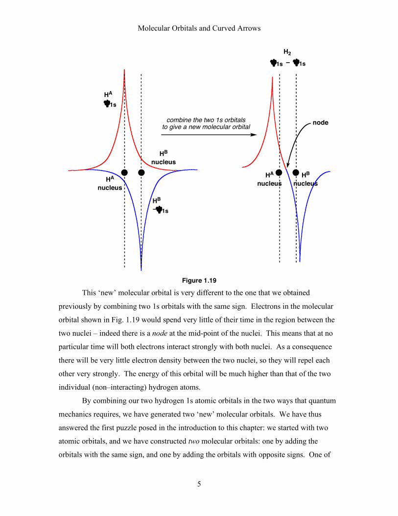
This ‘new’ molecular orbital is very different to the one that we obtained

previously by combining two 1s orbitals with the same sign. Electrons in the molecular

orbital shown in Fig. 1.19 would spend very little of their time in the region between the

two nuclei – indeed there is a node at the mid-point of the nuclei. This means that at no

particular time will both electrons interact strongly with both nuclei. As a consequence

there will be very little electron density between the two nuclei, so they will repel each

other very strongly. The energy of this orbital will be much higher than that of the two

individual (non–interacting) hydrogen atoms.

By combining our two hydrogen 1s atomic orbitals in the two ways that quantum

mechanics requires, we have generated two ‘new’ molecular orbitals. We have thus

answered the first puzzle posed in the introduction to this chapter: we started with two

atomic orbitals, and we have constructed two molecular orbitals: one by adding the

orbitals with the same sign, and one by adding the orbitals with opposite signs. One of


6

these is much lower in energy than the orbitals of the two isolated hydrogen atoms, and

the other is much higher in energy than the orbitals two isolated hydrogen atoms. We can

represent this using a simple ‘orbital energy diagram’ as shown in Fig. 1.20.

!1s !1s

H2

–

!1s !1s+

HA 1s HB 1s

H2

En

erg

y

These are the molecular orbitals thatresult from combining the two atomic orbitals

These are the atomic orbitals thatwe combined to make the molecular orbitals

How to read this type of orbital energy diagram:"If we take two hydrogen 1s orbitals and combine them to make molecular orbitals of the hydrogen molecule, we get two molecular orbitals. One of these is lower in energy than the 'starting' atomic orbitals and one is higher energy."

Figure 1.20

We will use this type of orbital energy diagram a lot and so it’s important that you

understand what it means. It is really a shorthand way of representing the fact that when

we combine the two atomic orbitals to make the ‘new’ molecular orbitals of the hydrogen

molecule, we get two molecular orbitals, one of which is lower in energy than the

original atomic orbitals and one of which is higher in energy than the original atomic

orbitals.

You might think that after all this we have not made much headway towards

explaining why the hydrogen atoms combine to make a hydrogen molecule. After all we

appear to have generated one new molecular orbital that is low energy and another that is

high energy, and so they should cancel each other out. However, this is not the case


7

because so far we have not assigned any electrons to the molecular orbitals. A key point

to remember about orbitals (atomic or molecular) is that an orbital only ‘counts’ towards

the energy of the system if it has one or two electrons in it. Empty orbitals (atomic or

molecular) contribute nothing to the energy – if they are devoid of electron density then

they are irrelevant with respect to the energy!

If this seems a little odd to you then consider a hydrogen atom. We know that

there are several allowed energy levels for the electron in a hydrogen atom, and that in its

ground state the electron is in the lowest (1s) energy level. The higher energy 2s orbital

is ‘available’ but empty and so makes no contribution to the energy. If we wanted to

promote the ground state electron to the 2s orbital we would need to provide just the right

amount of energy (ΔE in Fig. 1.21). If we did this then the resulting hydrogen atom

would not be in its ground state, and it would rapidly and spontaneously revert its ground

state – the electron would move to the 1s energy level emitting the energy that we

provided (Fig 1.21).

H 1s

En

erg

y

H 2s

H 1s

H 2s

H 1s

H 2s

!E

+ !E

ground statehydrogen atom

excited statehydrogen atom

ground statehydrogen atom

(~ 235 kcal mol–1)

– !E

(~ 235 kcal mol–1)

Figure 1.21

The electronic structure of the hydrogen molecule is analogous to that of the hydrogen

atom shown in Fig. 1.21 in that we have two orbitals (molecular orbitals of course), one

low energy and one high energy, and the ground state of the molecule will be that in

which the electrons occupy the lowest energy orbital. The rules for filling molecular

orbitals are no different to those for filling atomic orbitals – we fill the lowest energy


8

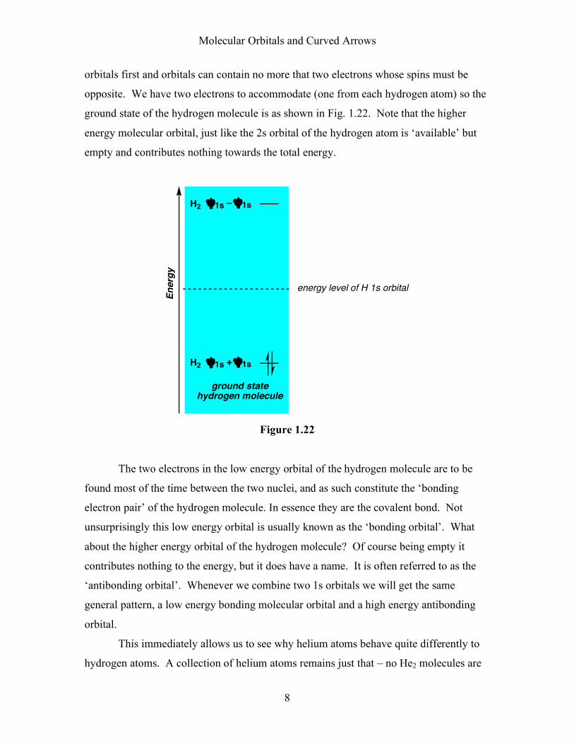
orbitals first and orbitals can contain no more that two electrons whose spins must be

opposite. We have two electrons to accommodate (one from each hydrogen atom) so the

ground state of the hydrogen molecule is as shown in Fig. 1.22. Note that the higher

energy molecular orbital, just like the 2s orbital of the hydrogen atom is ‘available’ but

empty and contributes nothing towards the total energy.

E

nerg

y

ground statehydrogen molecule

!1s !1s–

!1s !1s+H2

energy level of H 1s orbital

H2

Figure 1.22

The two electrons in the low energy orbital of the hydrogen molecule are to be

found most of the time between the two nuclei, and as such constitute the ‘bonding

electron pair’ of the hydrogen molecule. In essence they are the covalent bond. Not

unsurprisingly this low energy orbital is usually known as the ‘bonding orbital’. What

about the higher energy orbital of the hydrogen molecule? Of course being empty it

contributes nothing to the energy, but it does have a name. It is often referred to as the

‘antibonding orbital’. Whenever we combine two 1s orbitals we will get the same

general pattern, a low energy bonding molecular orbital and a high energy antibonding

orbital.

This immediately allows us to see why helium atoms behave quite differently to

hydrogen atoms. A collection of helium atoms remains just that – no He2 molecules are


9

formed. The two electrons in a ground state helium atom are both in the 1s level. If a

He2 molecule was to form, we would get the same pattern of molecular orbitals as for the

hydrogen molecule – a low energy bonding molecular orbital and a high energy

antibonding molecular orbital (Fig. 1.23). The molecular orbital pattern is the same as

for hydrogen but of course each helium atom has two electrons and so the helium

molecule would need to accommodate these four electrons in its available molecular

orbitals. This means that both the bonding and the antibonding molecular orbitals will be

filled. The energy of the bonding orbital is lowered less than that of the antibonding

orbital is raised (relative to the energy of the electrons in a helium atom), because in the

bonding orbital the electrons must stay close to each other and so there is more electron–

electron repulsion (in the antibonding orbital the electrons are on average much further

apart). All this means the helium molecule would be higher in energy than two isolated

helium atoms and so does not form spontaneously.

En

erg

y

molecular orbitals of the hypotheticalhelium molecule

!1s !1s–

!1s !1s+He2

energy levelof He 1s orbital

He2

En

erg

y

!1s !1s–

!1s !1s+He2

He2

Add 4 electrons

ground state of thehypothetical

helium molecule

"EB

"EA

"EA > "EB

– the molecule does not form Figure 1.23

We have spent quite a lot of time discussing hydrogen and helium, neither of

which is an organic compound! They are of course the simplest systems we could have


10

chosen to illustrate the important ideas behind covalent bonding. Very soon we will

study the bonding in organic molecules, but before that we will generalize the rules for

combining orbitals so that we can apply the ideas we developed in this section to organic

molecules in general.

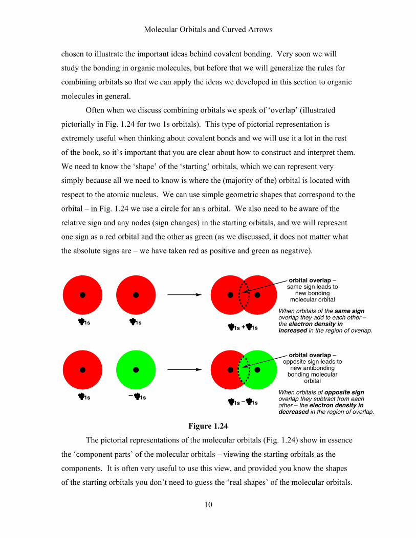
Often when we discuss combining orbitals we speak of ‘overlap’ (illustrated

pictorially in Fig. 1.24 for two 1s orbitals). This type of pictorial representation is

extremely useful when thinking about covalent bonds and we will use it a lot in the rest

of the book, so it’s important that you are clear about how to construct and interpret them.

We need to know the ‘shape’ of the ‘starting’ orbitals, which we can represent very

simply because all we need to know is where the (majority of the) orbital is located with

respect to the atomic nucleus. We can use simple geometric shapes that correspond to the

orbital – in Fig. 1.24 we use a circle for an s orbital. We also need to be aware of the

relative sign and any nodes (sign changes) in the starting orbitals, and we will represent

one sign as a red orbital and the other as green (as we discussed, it does not matter what

the absolute signs are – we have taken red as positive and green as negative).

!1s !1s!1s !1s+

orbital overlap – same sign leads to

new bonding molecular orbital

!1s – !1s!1s !1s–

orbital overlap – opposite sign leads to

new antibonding bonding molecular

orbital

When orbitals of the same sign overlap they add to each other – the electron density in increased in the region of overlap.

When orbitals of opposite sign overlap they subtract from each other – the electron density in decreased in the region of overlap.

Figure 1.24

The pictorial representations of the molecular orbitals (Fig. 1.24) show in essence

the ‘component parts’ of the molecular orbitals – viewing the starting orbitals as the

components. It is often very useful to use this view, and provided you know the shapes

of the starting orbitals you don’t need to guess the ‘real shapes’ of the molecular orbitals.


11

Sometimes it is useful and instructive to show these ‘real shapes’ and it is not difficult to

draw simple approximate shapes by considering where areas of electron density are

raised or lowered by the overlap. The relationship between the ‘component parts’ view

and ‘real shapes’ of the molecular orbitals from Fig. 1.24 is illustrated in Fig. 1.25.

!1s !1s+

orbital overlap – same sign leads to

new bonding molecular orbital

!1s !1s–

orbital overlap – opposite sign leads to

new antibonding bonding molecular

orbital

When orbitals of the same sign overlap they add to each other – the electron density in increased in the region of overlap.

When orbitals of opposite sign overlap they subtract from each other – the electron density in decreased in the region of overlap.

'component parts' representations 'real shape' representations

!1s !1s+

!1s !1s–

node

Figure 1.25

Now that you have seen the shapes of these bonding and antibonding orbitals, we

can offer a more intuitive explanation of why they are called “bonding” and

“antibonding.” The term “antibonding,” in particular, tends to cause much confusion

among chemistry students. Consider the simple “snapshot” of the H2 molecule that we

discussed in Chapter 1. Indeed, let us simplify the picture even further and consider the

H2+ molecular ion, which contains only one electron and two nuclei. If that electron is in

a bonding orbital, it is most likely to be found between the nuclei, where the

wavefunction is greatest. Thus, a likely “snapshot” of an electron in a bonding orbital

would be as follows:

'snapshot' of the hydrogen molecular ion (H2+)

with the electron in a bonding orbital

nucleus = electron =

electrostatic force on the nuclei

due to their attraction to the electron


12

Imagine that the electron in the above figure is momentarily “frozen” in this snapshot.

What will be the forces on the nuclei due to their attraction to the electron? The nucleus

on the left will feel a force toward the right (as indicated by the green arrow in the above

figure), while the nucleus on the right will feel a force toward the left. The result of these

two forces is that the nuclei are drawn closer together: the presence of electron density

between the nuclei pulls the nuclei together, resulting in a chemical bond. Thus, when a

molecular orbital has its greatest electron density between the nuclei, we call that orbital a

bonding orbital.

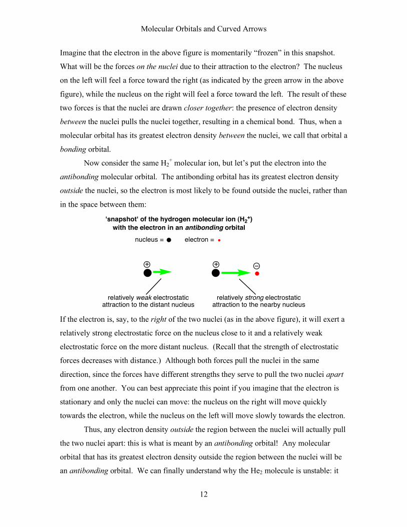
Now consider the same H2+ molecular ion, but let’s put the electron into the

antibonding molecular orbital. The antibonding orbital has its greatest electron density

outside the nuclei, so the electron is most likely to be found outside the nuclei, rather than

in the space between them:

'snapshot' of the hydrogen molecular ion (H2+)

with the electron in an antibonding orbital

nucleus = electron =

relatively strong electrostaticattraction to the nearby nucleus

relatively weak electrostaticattraction to the distant nucleus

If the electron is, say, to the right of the two nuclei (as in the above figure), it will exert a

relatively strong electrostatic force on the nucleus close to it and a relatively weak

electrostatic force on the more distant nucleus. (Recall that the strength of electrostatic

forces decreases with distance.) Although both forces pull the nuclei in the same

direction, since the forces have different strengths they serve to pull the two nuclei apart

from one another. You can best appreciate this point if you imagine that the electron is

stationary and only the nuclei can move: the nucleus on the right will move quickly

towards the electron, while the nucleus on the left will move slowly towards the electron.

Thus, any electron density outside the region between the nuclei will actually pull

the two nuclei apart: this is what is meant by an antibonding orbital! Any molecular

orbital that has its greatest electron density outside the region between the nuclei will be

an antibonding orbital. We can finally understand why the He2 molecule is unstable: it


13

has two electrons in a bonding orbital (pulling the nuclei together) and two electrons in

an antibonding orbital (pulling the nuclei apart), and the electrons in the antibonding

orbital win this “tug-of-war” and pull the two He atoms apart. This description of

bonding and antibonding orbitals is highly simplified; we discussed in Chapter 1 that the

electrons in an atom or molecule never sit still. The basic conclusion, however, is

correct: any electron density in a bonding orbital will hold the atoms together, while any

electron density in an antibonding orbital will pull the atoms apart.


14

2.2. Constructing Molecular Orbitals from Hybridized Orbitals

In this course, we will take an approach to molecular orbitals that may be

somewhat different from the approach used in your general chemistry course. We will

construct our molecular orbitals from atomic orbitals that are already hybridized. You

will find that it is simpler to make molecular orbitals out of hybridized orbitals than it is

to use unhybridized atomic orbitals. Note that, once you have hybridized the orbitals for

each atom, the only orbitals that can form molecular orbitals are hybridized orbitals

and leftover (unhybridized) p-orbitals.

The rules for making molecular orbitals (MO’s) out of hybridized orbitals are:

a) Hybridized orbitals can combine “end-on” to make sigma-type molecular orbitals.

b) Unhybridized p-orbitals can combine “side-on” to make pi-type molecular orbitals.

c) Each pair of orbitals combines to make a bonding MO and an antibonding MO.

Let’s look at some examples. First, recall the shapes of the orbitals:

node

region of(+) sign

region of(–) signhybridized orbital (sp, sp2, or sp3):

node

region of(–) sign

region of(+) sign

unhybridized p-orbital:

Note that the hybridized orbitals all have roughly the same shape: they each consist of

two “lobes,” one of which is much larger than the other. Between these two lobes, there

is a node: the two lobes have opposite signs, as indicated by the shaded (positive sign)


15

and unshaded (negative sign) regions. A p-orbital, on the other hand, has two lobes that

are the same size. As with the hybridized orbitals, there is a node between these lobes;

the two lobes are of opposite sign.

These orbitals combine to form molecular orbitals. We can combine two

hybridized orbitals to make a σ bonding orbital and a σ* antibonding orbital:

node

!* antibonding orbital

! bonding orbital

As discussed in the example of the covalent bonding in H2, the σ bonding orbital is

constructed from a combination of the two hybridized orbitals “in phase”—with the same

sign in the region between the nuclei. Thus, there is no node between the nuclei and the

bonding orbital has lower energy than the individual hybridized orbitals. Conversely, the

σ antibonding orbital is constructed from a combination of the two hybridized orbitals

“out of phase”—with opposite signs in the region between the nuclei. Thus, there is a

node—a region of zero electron density—between the nuclei. The antibonding orbital

therefore has higher energy than the individual hybridized orbitals.

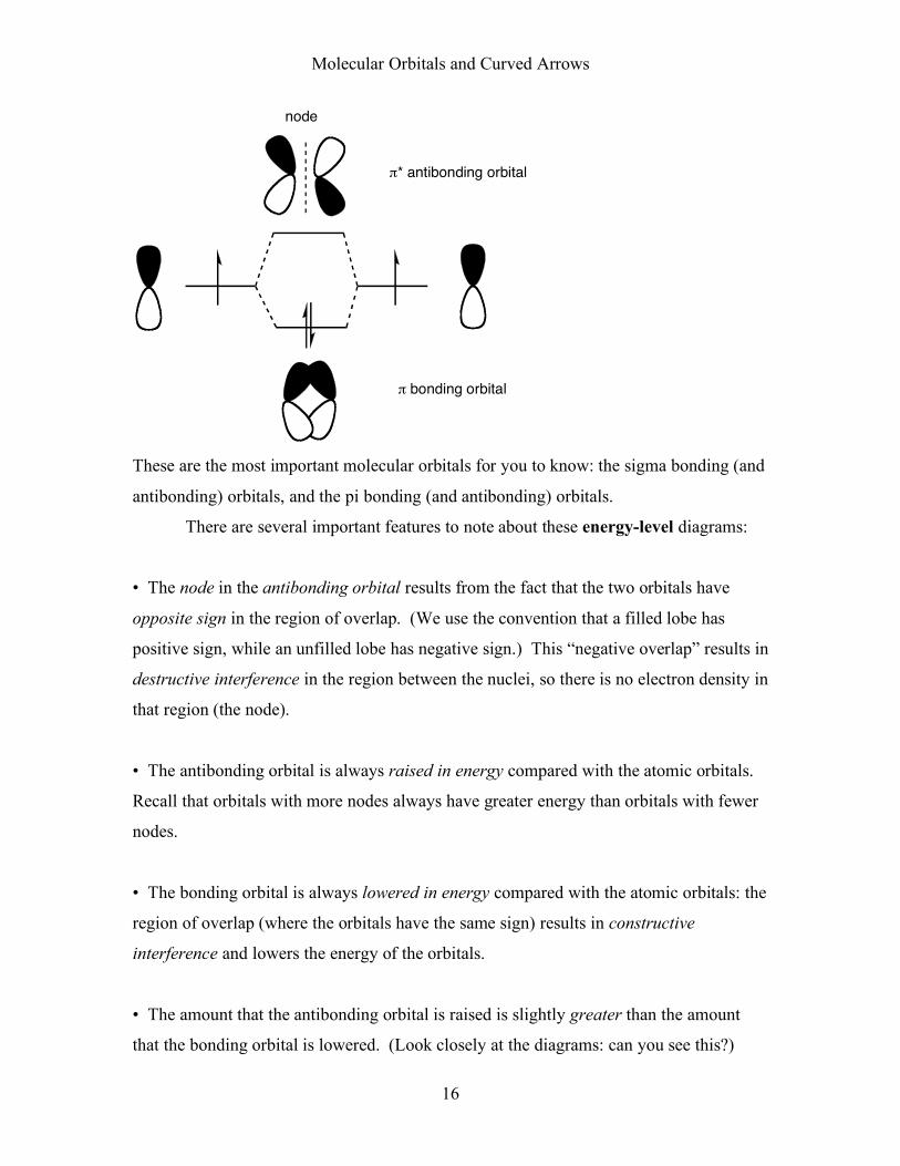
Instead of combining hybridized orbitals to create a σ-bond, we can combine

unhybridized p-orbitals to create a π-bond. The two p-orbitals combine to make a π

bonding orbital and a π* antibonding orbital:


16

node

!* antibonding orbital

! bonding orbital

These are the most important molecular orbitals for you to know: the sigma bonding (and

antibonding) orbitals, and the pi bonding (and antibonding) orbitals.

There are several important features to note about these energy-level diagrams:

• The node in the antibonding orbital results from the fact that the two orbitals have

opposite sign in the region of overlap. (We use the convention that a filled lobe has

positive sign, while an unfilled lobe has negative sign.) This “negative overlap” results in

destructive interference in the region between the nuclei, so there is no electron density in

that region (the node).

• The antibonding orbital is always raised in energy compared with the atomic orbitals.

Recall that orbitals with more nodes always have greater energy than orbitals with fewer

nodes.

• The bonding orbital is always lowered in energy compared with the atomic orbitals: the

region of overlap (where the orbitals have the same sign) results in constructive

interference and lowers the energy of the orbitals.

• The amount that the antibonding orbital is raised is slightly greater than the amount

that the bonding orbital is lowered. (Look closely at the diagrams: can you see this?)


17

• The amount of energy raising and lowering is greater for sigma bonds than for pi

bonds. This is because sigma bonds have better orbital overlap than pi bonds.

The amount of raising and lowering of the energies of the molecular orbitals is

primarily determined by two factors: the geometric overlap of the atomic orbitals, and the

difference in energy between the atomic orbitals. Let’s examine each of these important

factors:

First, consider the effect of geometric overlap. Imagine taking a molecule of

ethane (H3C–CH3) and stretching the C–C bond. What will happen to the energies of the

molecular orbitals as we stretch that bond?

H3C–CH3 --- stretch ----> H3C————CH3

C C

!C–C

!*C–C

poorer deconstructive interferencegives less "raising" of antibonding orbital

C C

!*C–C

!C–C

poorer constructive interferencegives less "lowering" of bonding orbital

We see that as we stretch the bond, the geometric overlap between the sp3-hybridized

orbitals becomes smaller and smaller, so the splitting in energy between the σ bonding

orbital and the σ* antibonding orbital decreases. If we streched the bond to an infinite

distance, there would be no splitting—and no bond!

Now, consider the effect of the difference in energy between the orbitals. Compare the

molecule Br2 (Br–Br), in which the two atomic orbitals have the same energy, with the

molecule ICl (I–Cl), in which the two atomic orbitals have different energies:


18

Br–Br I–Cl

Br Br

!Br–Br

!*Br–Br

I

Cl

!I–Cl

!*I–Cl

We see that orbitals that are close in energy give rise to a large change in energy

between the atomic orbitals and the resulting molecular orbitals. (Question: Why are the

chlorine orbitals lower in energy than the iodine orbitals?)

When the orbitals of the two atoms have different energies (e.g. they come from

atoms with different electronegativities), the resulting molecular orbital will be

asymmetric. Look at the asymmetric σ (sigma) orbitals in H3C–Cl, and the asymmetric π

(pi) orbitals in H2C=O:

H3C–Cl H2C=O

C

Cl

!C–Cl

!*C–Cllargerlobeon C

largerlobeon Cl

!*C=O

!C=O

C

O

largerlobeson C

largerlobeson O

The bonding orbital always has a larger lobe near the more electronegative atom (where

there is more electron density). Thus, the rules of quantum mechanics require that the

antibonding orbital must have a larger lobe near the less electronegative atom. In

both of the above diagrams, the antibonding orbital has a larger lobe on the carbon atom.

This asymmetry will be extremely important in determining how molecules react.


19

Practice Problem 2.2: Construct a simple molecular orbital “splitting diagram” for the

specified bonds in each of the following species. The splitting diagram should include

the atomic orbitals for the atoms involved in the bond and the resulting molecular

orbitals. Try to illustrate the correct relative energies of the orbitals involved. Include

“cartoon orbitals” that represent the general shape (and, when relevant, the asymmetry) of

the resulting molecular orbitals.

the C–Cl !-bond in CH3Cl

the C=C "-bond in H2C=CH2

the C=O "-bond in

the two C=N "-bonds in

the C–H !-bond in CH3Cl

O

H3C C N


20

2.2(a) The Energies of Atomic Orbitals

We learned in Chapter 1 that the electronegativity of an atom influences the

energies of its orbitals: more electronegative atoms have lower-energy orbitals. Since we

are constructing molecular orbitals from hybridized orbitals, we should also determine

how the hybridization of an atom affects the energies of its orbitals. Recall the energies

of the s and p orbitals we saw in Chapter 1:

Approximate energies (in kcal mol–1) of atomic orbitals

C

NO

F

2s

2p

2s

2p

2s

2p

2s

2p

0

100

200

300

400

500

600

700

800

900

1000

1100

Ne

2s

2p

0

100

200

300

400

500

600

700

800

900

1000

1100

We described hybridized orbitals as mixtures of the basic atomic orbitals. For instance,

an sp hybrid orbital is a mixture of one s-orbital and one p-orbital. Likewise, an sp3

hybrid orbital is a mixture of one s-orbital and three p-orbitals. In quantum mechanics,

when you mix atomic orbitals of different energy, the average energy of the mixed

orbital (technically called the “expectation value” of the energy”) is given simply by the

weighted average of the energies of the individual orbitals. So, the energy of an sp-


21

hybridized orbital is equal to the average of the energy of one s and one p orbital.

Consider oxygen as an example. The energies of the 2s and 2p orbitals in oxygen are 750

and 350 kcal/mol, respectively. An sp-hybridized orbital will have an energy that is the

average of these two energies:

energy of sp-hybridized oxygen orbital = (750+350)/2 = 550 kcal/mol

You will often hear chemists say that an sp-hybridized orbital is 50% s and 50% p in

character; these percentages correspond to the weights of the energies in the above

formula. Likewise, the energy of an sp3-hybridized orbital is equal to the average of the

energy of one s and three p orbitals:

energy of sp3-hybridized oxygen orbital = (750+350+350+350)/4 = 450 kcal/mol

Chemists often refer to an sp3-hybridized orbital as 25% s and 75% p in character; again,

these percentages correspond to the weights of the energies in the above formula. The

diagram below shows the approximate energies of the hybridized orbitals of oxygen in

comparison to the atomic orbitals:

Approximate energies (in kcal mol–1) of hybridized orbitals

O

2s

2p

0

100

200

300

400

500

600

700

800

900

0

100

200

300

400

500

600

700

800

900

sp-hybrid

sp2-hybridsp3-hybrid

average ofone s and one p

average ofone s and two p's

average ofone s and three p's

As you can see from this diagram, the sp2- and sp3-hybridized orbitals are fairly close in

energy, while the sp-hybridized orbital is significantly lower in energy than the other two.

The important take-home message is that hybridized orbitals with more s-character


22

are lower in energy than hybridized orbitals with more p-character. In other words,

for all atoms, the energies of their hybridized orbitals follow the order sp < sp2 < sp3.

You will sometimes hear chemists say that sp-hybridized atoms are effectively more

electronegative than sp3-hybridized atoms. This statement is reasonable, if somewhat

oversimplified: you can think of “electronegativity” as a measure of the energy of

electrons in an orbital, with more electronegative orbitals having lower energies.

We have now seen two factors that affect the energies of atomic orbitals:

electronegativity and hybridization. There is a third factor that is also quite significant:

the effect of charge on orbitals: specifically, the effect of formal charge. Atoms that

have a positive formal charge will have orbitals that are lower in energy, while atoms that

have a negative formal charge will have orbitals that are higher in energy. This trend

should make sense; an atom with a greater positive charge will have a greater

electrostatic attraction for its electrons, so their overall energy will be lower.

Confusingly, this trend is often expressed by saying that an atom with a positive formal

charge is more electronegative than a neutral atom, and an atom with a negative formal

charge is less electronegative than a neutral atom.

There are thus three factors that affect the energies of atomic orbitals:

electronegativity, hybridization, and formal charge. These factors are summarized in the

following table:

Low energy orbitals

result from:

High energy orbitals

result from:

Electronegativity high electronegativity low electronegativity

Hybridization sp-hybridization sp3-hybridization

Formal Charge positive formal charge negative formal charge

You should commit these trends to memory, but you should also understand (and be able

to explain) the reasons behind these trends.


23

2.3. Molecular Orbitals for Simple Molecules

Now that you can construct a molecular orbital for a particular bond in a

molecule, let’s learn how to determine all the important valence molecular orbitals for a

molecule. First we’ll walk through an example. Let’s determine all the molecular

orbitals for the molecule formaldehyde, H2C=O.

Step 1. Draw the Lewis structure for the molecule, including any important

resonance structures. Determine the hybridization of all the atoms in the structure.

H

C

H

O

Carbon: sp2

Oxygen: sp2

Step 2. Make a list of all the molecular orbitals in the molecule. For every bond

in the Lewis structure, there will be two molecular orbitals: a bonding orbital and an

antibonding orbital. In addition, every nonbonded orbital in the molecule will

correspond to a single nonbonded molecular orbital. (Lone pairs and vacant p-orbitals

are examples of nonbonded orbitals). At this point, count to make sure you have the

correct total number of molecular orbitals:

(Total # of orbitals) = (# of hydrogen atoms) + (4 × (# of other atoms))

Question: Can you explain where this formula comes from?

For formaldehyde, H2C=O, we have the following orbitals (in no particular order):

2 σC–H , 2 σ*C–H , σC–O , σ*C–O , πC=O , π*C=O , 2 nbO

Note that there are a total of 10 molecular orbitals = (2 H atoms) + 4 × (2 other atoms)

The nonbonding orbitals on O (nbO) are the two lone pairs on the oxygen atom.


24

Step 3. Group the orbitals together and rank their energies according to the

following general guidelines:

(High energy)

σ*

π*

nb

π

σ

(Low energy)

For formaldehyde, we obtain the following groups of orbitals, with a rough order of

energies:

(High energy)

σ* 2 σ*C–H , σ*C–O

π* π*C=O

nb 2 nbO

π πC=O

σ 2 σC–H , σC–O

(Low energy)


25

Step 4. Within each of the above groups, rank the energies of the orbitals based

on the electronegativities of the atoms involved. (Recall that more electronegative atoms

have orbitals that are lower in energy.) For formaldehyde, we obtain the following list of

orbitals, with an approximate ordering of energy levels:

(High energy)

σ* 2 σ*C–H

σ*C–O

π* π*C=O

nb 2 nbO

π πC=O

σ 2 σC–H

σC–O

(Low energy)


26

Step 5. Draw horizontal lines to represent each orbital, and fill the orbitals with

the correct number of electrons. (You may wish to refer back to the Lewis structure to

count the total number of valence electrons in the molecule. Formaldehyde has 12

valence electrons.) Be sure to add electrons starting with the lowest-energy molecular

orbital, and observe the Pauli principle (each orbital can have at most 2 electrons, with

opposite spins). This diagram shows all the valence orbitals in the molecule, ordered

based on energy, and filled with the correct number of electrons. It is usually called as an

“energy-level diagram.” You may wish to also draw “cartoon” representations of each

of the orbitals, just to remind yourself what each of the orbitals looks like.

(High energy)

2 !*C–H

!*C–O

"*C=O

2 nbO

"C=O

2 !C–H

!C–O (Low energy)


27

Step 6. Check your energy-level diagram:

• Does it have the correct number of orbitals?

• Does it have the correct number of electrons?

• Are all the bonding orbitals filled with electrons? (They should be!)

• Are all the antibonding orbitals vacant? (They should be!)

• Count the total number of filled bonding orbitals:

is that equal to the total number of bonds in the Lewis structure?

Practice Problem 2.3: For each of the following species, draw a complete Lewis

structure, showing all atoms and lone pairs, and then construct an energy-level diagram

for the valence molecular orbitals for the species. Be sure to check your MO diagram

using the guidelines given above!

O

OH

Cl

O

Br C N


28

2.4. Reactions Between Molecules: Frontier Orbitals

Now that we can determine all the molecular orbitals for a given molecule, we

can begin to answer the central question in chemistry: What happens when molecules

react, and why? Consider the following general chemical reaction:

A + B → C + D

You should visualize this reaction as follows: A molecule of A collides with a molecule

of B. Most of the time, those two molecules just bounce off of each other and emerge

unchanged. When A and B collide in the correct orientation with sufficient energy, they

can react during that collision, and molecules of C and D will emerge from the collision.

As an analogy, consider a pickpocket walking through a crowd. Most of the time, the

pickpocket bumps into someone and nothing happens. Sometimes, if the situation is just

right, the pickpocket bumps into someone and steals his wallet. After that collision, the

pickpocket now has the wallet and the victim does not. That type of collision, in which

the two species that emerge from the collision are different from those that entered the

collision, is analogous to a chemical reaction.

So, we want to ask: what happens when two molecules, A and B, collide? Well,

all of the orbitals of A interact with all of the orbitals of B molecule to form a whole set

of new orbitals. Then the electrons slosh around in all of these new orbitals and

redistribute themselves. Sometimes, the electrons can distribute themselves into new

orbitals that correspond to the products, C and D. In that case, these new products

emerge from the collision, and we say that a chemical reaction has occurred.

Although that description is generally accurate, it’s not very helpful to us in

determining what happens when molecules A and B collide. Each of these molecules

will have many molecular orbitals, and the number of interactions between those orbitals

will be an even larger number. Although computers can keep track of all those

interactions, you or I would have quite a hard time doing so. So we make a dramatic

simplification: we focus on the interactions between a very small number of orbitals,

known as the frontier orbitals. This approach, developed in the 1950’s by Kenichi

Fukui, of Kyoto University in Japan, and extended in the 1960’s by Roald Hoffmann, of


29

Cornell University, in Ithaca, New York, was so important that these two scientists

received the Nobel Prize in Chemistry in 1981 for their work. Understanding the

interactions of frontier orbitals is the key to understanding chemical reactivity.

Here are some excerpts from the press release of the 1981 Nobel Prize Committee

(emphasis added):

The Prizewinners' work aims at theoretically anticipating the course of chemical reactions. It is based on quantum mechanics (the theory whose starting point is that the smallest building blocks of matter may be regarded both as particles and as waves), which attempts to explain how atoms behave... [In the 1950’s], Fukui showed that certain properties of the orbits of the most loosely bound electrons and of the “most easily accessible” unoccupied electronic orbits had unexpectedly great significance for the chemical reactivity of molecules. He called these orbits “frontier orbitals.” Fukui's earlier frontier orbital theory attracted only little attention at first. In the mid-1960s, Fukui and Hoffmann discovered—almost simultaneously and independently of each other—that symmetry properties of frontier orbitals could explain certain reaction courses that had previously been difficult to understand. This gave rise to unusually intensive research activity—both theoretical and practical—in many parts of the world, as Fukui and other researchers developed the frontier orbital theory into a highly powerful tool for understanding the reactivity of molecules... A characteristic feature of Fukui's and Hoffmann's method of attacking difficult and complicated problems is that they succeeded in making generalizations through simplifications. In this lies the key to the strength of their theories. The theoretical models that Fukui and Hoffmann introduced have been in many branches of chemistry since the 1970s. Their method of conceiving of the course of chemical reactions is utilized nowadays, for example, by chemists studying life processes and by chemists making new drugs.

Kenichi Fukui Roald Hoffmann


30

For you, as a student, the most important message is that the theory of frontier orbitals

will allow you to anticipate the course of chemical reactions. That means that you can

predict what will happen in an organic reaction—you don’t have to memorize every

reaction. Let’s see how to use this amazing tool!

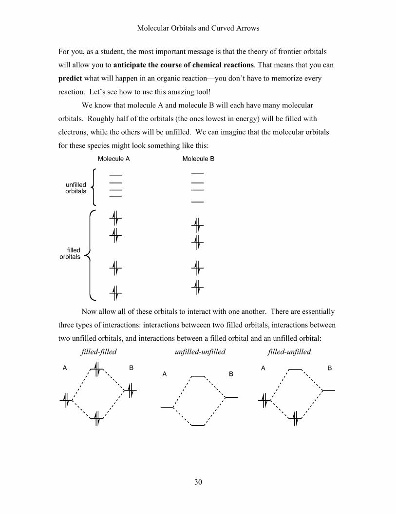
We know that molecule A and molecule B will each have many molecular

orbitals. Roughly half of the orbitals (the ones lowest in energy) will be filled with

electrons, while the others will be unfilled. We can imagine that the molecular orbitals

for these species might look something like this:

Molecule A Molecule B

unfilled

orbitals

filled

orbitals

Now allow all of these orbitals to interact with one another. There are essentially

three types of interactions: interactions betweeen two filled orbitals, interactions between

two unfilled orbitals, and interactions between a filled orbital and an unfilled orbital:

filled-filled unfilled-unfilled filled-unfilled

A B

A B

A B


31

When two filled orbitals interact, two electrons go up in energy and two electrons

go down in energy, but the total energy of the electrons doesn’t change very much. In

fact, the antibonding orbital is raised in energy more than the bonding orbital is lowered

in energy, so the total energy is actually increased: this is an unfavorable interaction.

When two unfilled orbitals interact, no electrons change energy at all, so this interaction

has no effect on the reaction. However, when a filled orbital interacts with an unfilled

orbital, the result is a net lowering of the total energy of the electrons. This observation

is the first rule of frontier orbitals: the most important interactions are those between

a filled orbital and an unfilled orbital. We can usually ignore all the other interactions.

Now consider all of the possible interactions between filled orbitals and unfilled

orbitals. We learned earlier that large splittings in the energy between the bonding and

antibonding orbitals result from two factors: orbitals that have favorable geometric

overlap and orbitals that are are close in energy. The issue of geometric overlap is

absolutely important: if two orbitals can’t overlap, they can’t interact. Recall, though,

that two molecules can collide in many different orientations. Often, at least one of those

orientations will allow the orbitals in question to overlap. So we must consider the

energies of the orbitals. If two orbitals are close in energy, there will be a large splitting

between the bonding and antibonding orbitals. For an interaction between filled and

unfilled orbitals, a large splitting will lead to a large lowering of the energy of the

electrons. Consider two possible interactions between a filled orbital from molecule A

and an unfilled orbital from molecule B:

Close in energy Not close in energy

Large loweringof the energy of these electrons

A B

Small loweringof the energy

of these electrons

A B

When the filled and unfilled orbitals are close in energy, the electrons in the filled

orbital end up significantly lower in energy; when the filled and unfilled orbitals have


32

very different energies, the electrons in the filled orbital end up only slightly lower in

energy.

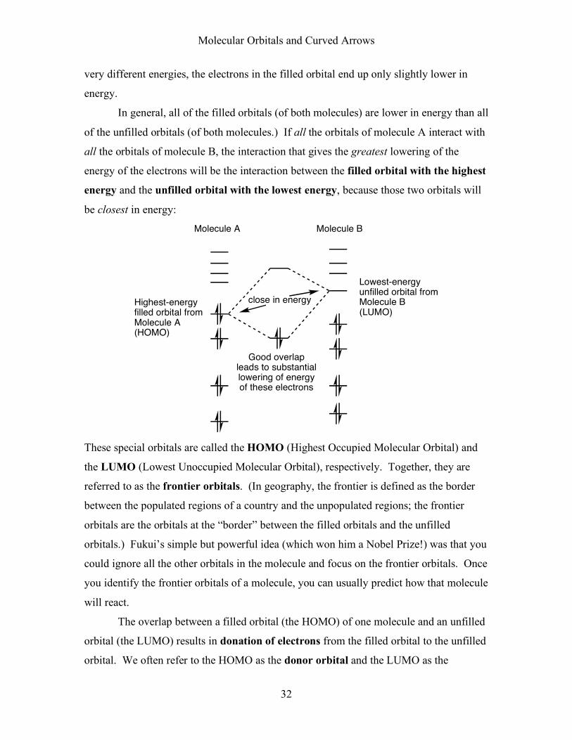
In general, all of the filled orbitals (of both molecules) are lower in energy than all

of the unfilled orbitals (of both molecules.) If all the orbitals of molecule A interact with

all the orbitals of molecule B, the interaction that gives the greatest lowering of the

energy of the electrons will be the interaction between the filled orbital with the highest

energy and the unfilled orbital with the lowest energy, because those two orbitals will

be closest in energy:

Molecule A Molecule B

Highest-energyfilled orbital fromMolecule A(HOMO)

Lowest-energyunfilled orbital fromMolecule B(LUMO)

close in energy

Good overlapleads to substantiallowering of energyof these electrons

These special orbitals are called the HOMO (Highest Occupied Molecular Orbital) and

the LUMO (Lowest Unoccupied Molecular Orbital), respectively. Together, they are

referred to as the frontier orbitals. (In geography, the frontier is defined as the border

between the populated regions of a country and the unpopulated regions; the frontier

orbitals are the orbitals at the “border” between the filled orbitals and the unfilled

orbitals.) Fukui’s simple but powerful idea (which won him a Nobel Prize!) was that you

could ignore all the other orbitals in the molecule and focus on the frontier orbitals. Once

you identify the frontier orbitals of a molecule, you can usually predict how that molecule

will react.

The overlap between a filled orbital (the HOMO) of one molecule and an unfilled

orbital (the LUMO) results in donation of electrons from the filled orbital to the unfilled

orbital. We often refer to the HOMO as the donor orbital and the LUMO as the


33

acceptor orbital. These terms emphasize the roles that these orbitals play in a particular

reaction: the electron-rich donor orbital donates electrons into the vacant acceptor orbital.

The key question in predicting and understanding the results of the reaction between two

molecules can be stated quite simply: Which orbital will be the donor, and which orbital

will be the acceptor? Once that question is answered, you can usually predict the course

of the reaction: the donor orbital will donate electrons to the acceptor orbital. Nothing

could be simpler!

One of the most important skills, then, is to be able to identify quickly the frontier

orbitals (the donor and acceptor orbitals) in any organic molecule. You can always write

out a complete energy-level diagram, as you did in Section 2.3, and find the highest

occupied MO and the lowest unoccupied MO from the diagram. There are some simple

“shortcuts,” however, that can allow you to find all the reasonable candidates for the

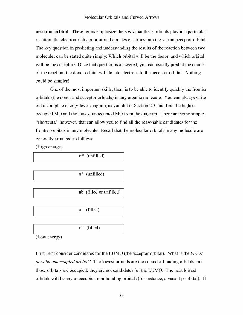
frontier orbitals in any molecule. Recall that the molecular orbitals in any molecule are

generally arranged as follows:

(High energy)

σ* (unfilled)

π* (unfilled)

nb (filled or unfilled)

π (filled)

σ (filled)

(Low energy)

First, let’s consider candidates for the LUMO (the acceptor orbital). What is the lowest

possible unoccupied orbital? The lowest orbitals are the σ- and π-bonding orbitals, but

those orbitals are occupied: they are not candidates for the LUMO. The next lowest

orbitals will be any unoccupied non-bonding orbitals (for instance, a vacant p-orbital). If


34

a molecule has a vacant non-bonding orbital, that orbital is almost always the LUMO.

Otherwise, the LUMO must be an antibonding orbital. Recall that more electronegative

orbitals are lower in energy. Thus, the LUMO is likely to be a π* or σ* antibonding

orbital that involves an electronegative atom—for instance, a π*C=O or σ*C–Br orbital.

Next, consider candidates for the HOMO (the donor orbital). What is the highest

possible occupied orbital? The highest-energy orbitals are the σ*- and π*-antibonding

orbitals, but these orbitals do not contain any electrons: they are not candidates for the

HOMO. For organic molecules, the HOMO is almost always a lone pair (a filled non-

bonding orbital). Sometimes, the HOMO may be a filled π-orbital. Because orbitals

involving electronegative atoms are low in energy, the HOMO is likely to be a filled π-

orbital that does not have electronegative atoms—typically, a πC=C orbital. The following

table summarizes the likely HOMO’s and LUMO’s for organic molecules:

Best candidates for HOMO (donor) Best candidates for LUMO (acceptor)

1. Lone pairs (filled non-bonding orbitals) 1. Vacant p-orbital (non-bonding orbital)

2. π bonding orbitals: πC=C 2. π* antibonding orbitals (electroneg.)

3. σ* antibonding orbitals (electroneg.)

You should become adept at identifying the likely donor and acceptor orbitals

simply by looking at the skeletal structures of organic molecules. Let’s take a look at

some examples. Notice that we indicate all the potential donors and potential acceptors

for a given molecule. Our goal is not to identify the single orbital in a molecule that will

interact, but rather to identify the plausible candidates based on the above table. Here are

some examples of molecules with plausible donors and acceptors identified:


35

Br

Acceptor: !*C–Br

Donor: Br lone pairs

H

O

Acceptor: "*C=O

Donor: O lone pairs

O

Acceptor: "*C=O or !*C–Cl

Donor: O lone pairs or Cl lone pairs

Cl

O

Acceptor: !*C–O

Donor: O lone pairs

Why do we identify more than one plausible donor for a molecule? Doesn’t the

word “highest” in HOMO mean that there is only one HOMO, which should be the best

donor orbital for that molecule? Yes, but you must also consider the geometry of the

molecule and its interaction with other molecules. For instance, consider the following

molecule:

OH

Donor: !C=C Donor: O lone pairs

This molecule has two plausible donors: the oxygen lone pair and the alkene πC=C.

Why? The oxygen lone pair is the HOMO for this molecule: it is certainly higher in

energy than the π-bonding orbital. You must also consider the geometry of the

interaction, however. If another molecule collides with the left end of this molecule, then

it will only “see” the π-bond, and it will react with that donor orbital as if it were the

HOMO. If another molecule collides with the right end of this molecule, it will “see” the

oxygen lone pair, and will react with that donor orbital:

OH

a collision with

this end of the moleculewould "see" the!C=C as the donor

a collision withthis end of the moleculewould "see" theO lone pairs as the donor


36

So the apparently simple question of “what is the best donor orbital for that molecule?”

often must be answered: “It depends on how another molecule interacts with that

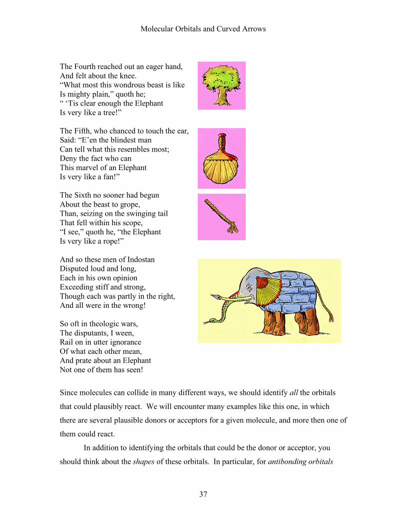
molecule!” As an analogy, consider the famous poem about the “blind men and the

elephant,” by American poet John Godfrey Saxe (1816-1887):

It was six men of Indostan To learning much inclined, Who went to see the Elephant (Though all of them were blind), That each by observation Might satisfy his mind The First approached the Elephant, And happening to fall Against his broad and sturdy side, At once began to bawl: “God bless me! but the Elephant Is very like a wall!” The Second, feeling of the tusk, Cried, “Ho! what have we here So very round and smooth and sharp? To me ’tis mighty clear This wonder of an Elephant Is very like a spear!” The Third approached the animal, And happening to take The squirming trunk within his hands, Thus boldly up and spake: “I see,” quoth he, “the Elephant Is very like a snake!”


37

The Fourth reached out an eager hand, And felt about the knee. “What most this wondrous beast is like Is mighty plain,” quoth he; “ ‘Tis clear enough the Elephant Is very like a tree!” The Fifth, who chanced to touch the ear, Said: “E’en the blindest man Can tell what this resembles most; Deny the fact who can This marvel of an Elephant Is very like a fan!” The Sixth no sooner had begun About the beast to grope, Than, seizing on the swinging tail That fell within his scope, “I see,” quoth he, “the Elephant Is very like a rope!” And so these men of Indostan Disputed loud and long, Each in his own opinion Exceeding stiff and strong, Though each was partly in the right, And all were in the wrong! So oft in theologic wars, The disputants, I ween, Rail on in utter ignorance Of what each other mean, And prate about an Elephant Not one of them has seen!

Since molecules can collide in many different ways, we should identify all the orbitals

that could plausibly react. We will encounter many examples like this one, in which

there are several plausible donors or acceptors for a given molecule, and more then one of

them could react.

In addition to identifying the orbitals that could be the donor or acceptor, you

should think about the shapes of these orbitals. In particular, for antibonding orbitals


38

that are potential acceptors, you should note that the largest lobe of the orbital is actually

“behind” the less electronegative atom. Here are some examples of molecules with

antibonding orbitals as their LUMO in which the most important lobe is indicated. (For

π* orbitals, of course, there are two such lobes, above and below the plane of the paper.)

Br

lobe ofLUMO!*C–Br

O

two equivalent!*C–O

LUMO's

C N

N

one of thelobes of LUMO"*C=N

side viewof "*C=N

LUMO

largelobes of"*C=N

CH

O

H

O

one of thelobes of LUMO"*C=O

side viewof "*C=O

LUMO

largelobes of"*C=O


39

Practice Problem 2.4: For each of the following molecules, circle the plausible donors

and acceptors and provide their names (e.g. σ*C–Br , πC=C , etc.). (In the case of an

antibonding acceptor orbital, do not circle the bond; instead, draw a circle that represents

the largest lobe of the acceptor orbital as discussed above.)

O

H

O

O

BrC N


40

2.5. Reactions Between Molecules: Frontier Orbitals and Curved Arrows

You now have the skills to:

• List all the molecular orbitals in a molecule

• Draw the shapes of these orbitals

• Estimate the order of energies of these orbitals

• Identify the possible frontier orbitals (donor and acceptor)

Now you can learn how the frontier orbitals of two molecules interact. First, we need to

introduce a bit of important terminology. In the simplest organic reactions, the (filled)

donor orbital of one molecule will react with the (empty) acceptor orbital of the other

molecule. In such a reaction, the molecule that is providing the electrons—the one with

the donor—is called the nucleophile, while the molecule with a vacant orbital that can

accept electrons—the one with the acceptor—is called the electrophile. These two

words, nucleophile and electrophile, are derived from the words “nucleus” or “electron”

along with the Greek suffix “philos,” meanining “friend of” or “love of.” An

electrophile, with its vacant orbital, has a “love of” electrons, while a nucleophile, with

its orbital full of high-energy electrons, has a “love of” the (positively-charged) nucleus.

A nucleophile has electrons that it wants to share or donate, and an electrophile wants

electrons.

Note that the terms HOMO and LUMO refer to orbitals, while the terms

electrophile and nucleophile refer to molecules. To be more specific, the terms

electrophile and nucleophile refer to the role that a molecule plays in a given interaction.

A molecule could be a nucleophile in one reaction and an electrophile in another. As an

analogy, the terms “buyer” and “seller” refer to the role that a person plays in an

economic transaction. When I go to a car dealer to buy a new car, I play the role of

buyer, and the car dealer is the seller. When the car is old and I want to get rid of it, I can

go back to the dealer and sell it back as a used car; now I am the seller and the dealer is

the buyer. The terms electrophile and nucleophile are analogous: the nucleophile is often

referred to as the electron donor in a reaction, while the electrophile is the electron

acceptor.


41

In analyzing a reaction between two molecules, you must decide which molecule

will act as the nucleophile and which will act as the electrophile. Usually, the molecule

with the “highest HOMO” (i.e. the highest-energy donor orbital) will be the nucleophile,

and the molecule with the “lowest LUMO” (i.e. the lowest-energy acceptor orbital) will

be the electrophile. Likewise, molecules with a negative charge (anions) are likely to be

nucleophiles, while molecules with a positive charge (cations) are likely to be

electrophiles. (Note that we use the term “molecule” as a general term that can refer to

either neutral or charged species.)

You can now learn how to predict what will happen when two molecules react

with one another. The general strategy is:

1. Identify the plausible donor and acceptor orbitals for the molecules.

2. Choose one molecule to be the nucleophile and the other to be the electrophile.

3. Have the donor orbital of the nucleophile react with the acceptor orbital of the

electrophile.

What does it mean for the donor to “react with” the acceptor? That phrase means that

electrons from the donor orbital “flow” or “donate” into the acceptor orbital. To keep

track of this flow of electrons, organic chemists use a simple but powerful tool known as

cuvred arrows; the process of drawing curved arrows to keep track of the flow of

electrons is often called arrow pushing. Let’s look at some examples.


42

• Reaction between a non-bonding donor (lone pair) and a non-bonding acceptor:

This is the simplest type of frontier orbital interaction. Consider, as an example,

the reaction between the chloride ion Cl– and the tert-butyl cation, (H3C)3C+. First, we

must draw the Lewis structures and identify the plausible donor and acceptor orbitals for

these species:

Cl

CH3

CH3H3C

HOMO: Cl lone pair LUMO: nonbonding p orbitalon positively-charged carbon atom

C

CH3

CH3H3C

(This is the complete Lewisstructure of the cation)

We can use curved arrows to show the flow of electrons from the donor (HOMO) to the

acceptor (LUMO). This donation of electrons results in the formation of a new bond:

Cl

CH3

CH3H3C

Cl

CH3

CH3

CH3

new bond Keep in mind the orbitals involved here:

Cl CH3H3CH3C

lone pair donor vacant orbital acceptor

That’s it! That’s one of the simplest reactions in organic chemistry. In this example,

there is no ambiguity: the chloride ion has only one possible donor, and the cation has

one obvious acceptor. Also note that the combination of two non-bonding orbitals results

in one new bond (which has a bonding orbital and an antibonding orbital). (Recall that a

combination of n orbitals must yield n molecular orbitals.) This reaction is:

(lone pair) + (vacant orbital) → (new bond)


43

• Reaction between a non-bonding donor (lone pair) and an antibonding acceptor:

This is an extremely common type of frontier orbital interaction in organic

chemistry. As an example, consider the reaction between the hydroxide ion (OH–) and

methyl bromide (CH3Br). Again, we must first draw Lewis structures and identify the

frontier orbitals:

HO

HOMO: O lone pairLUMO: !*C–Br

HOMO: Br lone pairs (not shown)

C Br

H

HH

HO C Br

H

HH

(largest lobe of !*orbitalis behind the carbon atom!)

We use curved arrows to show the flow of electrons from the donor into the acceptor.

The electrons from the donor interact with the large lobe of the acceptor (the lobe

“behind” the carbon atom). In addition, note that donating electrons into an

antibonding orbital breaks the bond that is associated with that orbital: EXPAND!!

HO C Br

H

H

H

CHO

H

H

H

+ Br

In this reaction, the HOMO of OH– must overlap with the LUMO of CH3Br:

HO C Br

H

HH

CHO

H

HH

+ Br

new bond new lone pair Observe how the curved arrows help to keep track of where the electrons are going. This

reaction can be thought of as:

(lone pair) + (antibonding orbital) → (new bond) + (new lone pair)


44

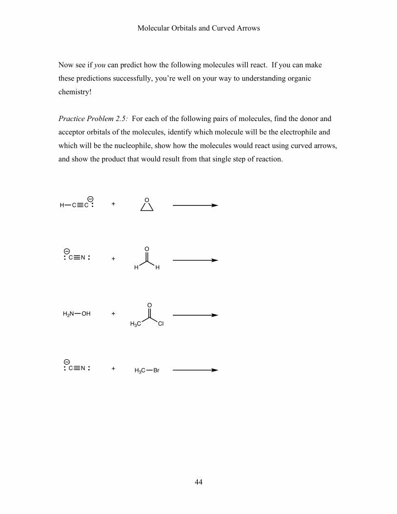
Now see if you can predict how the following molecules will react. If you can make

these predictions successfully, you’re well on your way to understanding organic

chemistry!

Practice Problem 2.5: For each of the following pairs of molecules, find the donor and

acceptor orbitals of the molecules, identify which molecule will be the electrophile and

which will be the nucleophile, show how the molecules would react using curved arrows,

and show the product that would result from that single step of reaction.

H C C +O

+

+

+

C N

H2N OH

C N

H H

O

H3C Cl

O

H3C Br


45

2.6. Proton-Transfer Reactions: Frontier Orbitals of Brønsted Acids and Bases

In your previous chemistry courses, you encountered the concept of acids and

bases. One of the most commonly-used definitions of acids and bases is known as the

Brønsted-Lowry acid-base theory. In this theory, an acid is defined as a species that can

donate a proton (H+), while a base is defined as a species that can accept a proton.

One of the basic concepts of this theory is that every acid has a conjugate base that

results from the “loss” of a proton from that acid. Here are some common Brønsted acids

and their conugate bases:

Brønsted Acid Conjugate Base

H2O OH–

H3O+ H2O NH4

+ NH3

H2S HS–

HF F–

HCl Cl–

Conversely, every Brønsted base has a conjugate acid that results from adding a proton

to that base. Here are some common Brønsted bases and their conjugate acids:

Brønsted Base Conjugate Acid

OH– H2O

H2O H3O+

NH3 NH4

+

HS– H2S

F– HF

Cl– HCl

You may notice that the above lists are quite similar! Every Brønsted acid is the

conjugate acid of a Brønsted base, and every Brønsted base is the conjugate base of a

Brønsted acid.

When a Brønsted acid reacts with a Brønsted base, a proton (H+) can be

transferred from the acid to the base. Such a reaction is called a proton-transfer

reaction. Here are some examples of proton-transfer reactions:

HF + NH3 F– + NH4+


46

NH4+ + OH– NH3 + H2O

H2S + OH– SH– + H2O

The products of any proton-transfer reaction are the conjugate acid and conjugate base

of the reactants. For example, in the reaction:

HF + NH3 F– + NH4+

the product F– is the conjugate base of the acid HF, and the product NH4+ is the conjugate

acid of the base NH3.

The nature of a proton-transfer reaction can be seen more clearly if we write out

the complete Lewis structures for the reactants and products. For instance, for the

reaction between the ammonium ion and the hydroxide ion:

NH4+ + OH– NH3 + H2O

the complete Lewis structures are:

N

H

H

H

H

+ O HN

HH

H

+ O H

H

If you write out the Lewis structures for any Brønsted proton-transfer reaction, you will

notice that Brønsted bases always have lone pairs, and it is the lone pair on the

Brønsted base that accepts the proton from the Brønsted acid.

We can use curved arrows to follow the motion of the electrons in an acid-base

reaction. (From now on in the text, when we use the generic terms “acid” or “base,” we

always mean “Brønsted acid” or “Brønsted base.”) For the reaction between the

ammonium ion and the hydroxide ion, the curved arrows are:

N

H

H

H

H

+ O HN

HH

H

+ O H

H

Note that the arrows follow the motion of the electrons, not the motion of the proton that

is being transferred! You should be able to identify the frontier orbitals of these species

and explain the reaction in terms of a donor-acceptor interaction. The frontier orbitals of

the reactants are:


47

NH

H

H

H

+ O H

Donor:

!*H–N

Acceptor:O lone pair

The hydroxide ion (OH–) is the nucleophile, with a lone pair as its donor orbital; the

ammonium ion (NH4+) is the electrophile, with a σ* antibonding orbital as its acceptor.

Note that the largest lobe of the antibonding orbital is, as usual, behind the less

electronegative atom (the hydrogen atom). As the curved arrows show, the donation of

electrons from the HOMO (donor orbital) of OH– into the antibonding σ*H–N orbital

breaks the H–N bond.

We can define Brønsted acids and bases in terms of their frontier orbitals:

• A Brønsted acid has a σ*H–Y orbital as an acceptor orbital, in which Y is an atom that is

more electronegative than H. It will transfer that proton when a filled orbital donates into

that vacant antibonding orbital.

• A Brønsted base has a filled orbital (usually a lone pair) as a donor orbital that can

accept a proton. It will accept a proton when that filled orbital donates into the σ*H–Y

antibonding orbital of a Brønsted acid.

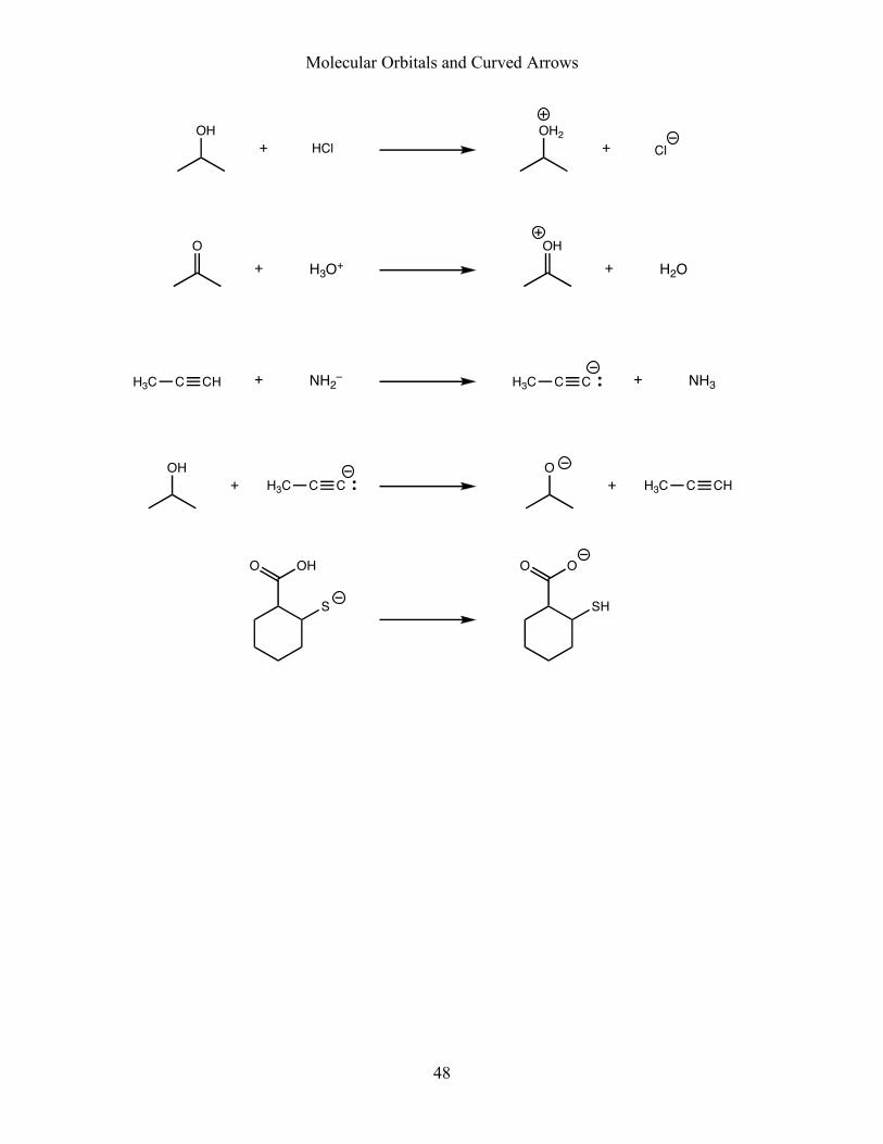
Practice Problem 2.6: For each of the following acid-base reactions, draw complete

Lewis structures of the reactants, draw curved arrows to explain the proton transfer that

occurs, and identify the HOMO and LUMO involved in the proton transfer.


48

OH

+ HCl

OH2

+ Cl

O

+ H3O+

OH

+ H2O

H3C C CH + NH2–

H3C C C + NH3

OH

+ H3C C C

O

+ H3C C CH

OHO

S

OO

SH


49

2.7. Electrophiles, Nucleophiles, Acids, and Bases

We have discussed two roles that a molecule can play in a chemical reaction:

• An electrophile is a molecule with a low-energy acceptor orbital that accepts electrons

into that orbital from a donor orbital of another species.

• A nucleophile is a molecule with a high-energy donor orbital that donates electrons

from that orbital into the acceptor orbital of some other species.

Although a Brønsted acid is merely a special type of electrophile (in which the

acceptor orbital is a σ*H–Y antibonding orbital), you should consider such an acid to be in

a category by itself. We will use the classical definition of a Brønsted acid as a proton

donor, although we understand that it is a proton donor because it has a σ*H–Y

antibonding orbital.

Likewise, although a Brønsted base is merely a special type of nucleophile (in

which the donor orbital of the nucleophile donates into a σ*H–Y antibonding orbital and

acquires the proton from that antibonding orbital), you should consider such a base to be

in a category by itself. We think of a base as a proton acceptor, but we understand that it

can accept a proton because it has a donor orbital that can donate into a σ*H–Y

antibonding orbital of another molecule (the Brønsted acid).

In any organic reaction, each molecule usually plays one of the above four roles:

the molecule acts as an electrophile, as a nucleophile, as an acid, or as a base. Indeed, the

main questions you should ask upon encountering any molecule or any reaction are the

four basic questions of organic reactivity:

• Can the molecule act as an electrophile?

• Can the molecule act as a nucleophile?

• Can the molecule act as an acid?

• Can the molecule act as a base?

Once you have answered those basic questions, you have an excellent chance of being

able to predict how that molecule will react: electrophiles react with nucleophiles, and

acids react with bases.


50

We conclude this chapter by examining some molecules that can exhibit different

reactivity depending on their role as an electrophile, nucleophile, acid, or base. See if

you can identify the role that each species is playing in the following reactions:

Practice Problem 2.7: For each of the following reactions:

• Draw the curved arrows that show how the reaction takes place.

• Identify the donor and acceptor orbitals of the interacting species.

• Identify each species as an electrophile, a nucleophile, an acid, or a base.

(Be sure to consider the role that the species is playing in the reaction!)

• Notice that the same species can play different roles in different reactions!


51

H3C CH3

CH3

+ H2O

H3C CH2

CH3

+ H3O+

H3C CH3

CH3

+ H2O

H3C CH3

CH3

OH2

S C N + H3O+S C N

H

S C N + H3C Br S C N

H3C

+ Br–

H3C CH3

O

H3C CH3

OH

H3C CH3

O

H3C CH3

O

H3C CH3

O

H3C CH3

H3C CH3

O

H3C CH2

O

+ H3O+ + H2O

O OH

CH3

O

CH3

H3C CH3

+O

H3C CH3

+

+ HO–

+ HO– + H2O

molecular orbitals handout

Documents