molecular interaction models - helsinki

Introduction to atomistic simulations 2008 10. Potential models for molecules and hydrocarbons 1

Set the initial conditions , ri

t0

! vi

t0

!

Get new forces Fir

i !

Solve the equations of motion numerically over time step :

"tr

itn

! ri

tn 1+

!# vi

tn

! vi

tn 1+

!#

t t "t+#

Get desired physical quantities

t tmax

?$ Calculate results

and finish

Update neighborlist

Perform , scaling (ensembles)T P

Potential

models for

molecules (and

hydrocarbons)


Molecular interaction models

• Since molecules are bonded by covalent bonds, at least angular terms are needed, • In many cases many more complicated terms as well: e.g. carbon chains the difference between “single”

and “double” bonds often is important %&at least a four-body term is needed. &

• To describe complex molecules a large set of force fields have been developed.• Molecular mechanics: use of force fields, no reactions (i.e. bond breaking or creation)

• Fixed neighbor topology (except for so called non-bonded interactions).&

• The total energy of a molecule can be given asE

bond

Eangle

Etorsion

Eoop

&

E Ebond

Eangle

Etorsion

Eoop

Ecross

Enonbond

+ + + + += &

Ebond

: energy change related to a change of bond length (V2

)&

Eangle

: energy change associated with a change in the bond angle,(V3

)&

Etorsion

: torsion, i.e. energy associated with the rotation between two parts &

of a molecule relative to each other (also termed dihedral)&

Eoop

: “out-of-plane” interactions, i.e. the energy change when one part &

of a molecule is out of the plane with another (keeps the molecule planar)&

Ecross

: cross terms between the other interaction terms&

Enonbond

: interaction energies which are not associated with covalent bonding (e.g.

ionic or van der Waals terms)&

• In the following we describe the terms, using notation more common on chemistry rather than

the physics notation used earlier on the course.



• The term Ebond

• This term describes the energy change associated with the bond length. It is a simple pair potential, and

could be e.g. a Morse or LJ potential.• At its simplest, it is purely harmonic, i.e.

Ebond

1

2---k

bb b

0–! "

2

bonds

#=

where b is the bond length.

• If we write this term instead as

Ei

12---k r

ijr0–! "

2

j

#=

we see that it is the same thing as the pair potentials dealt with earlier.

• Can be good enough in problems where we are always close to equilibrium, since any

smooth potential well can always be to the first order approximated by a harmonic

well.

• But harmonic potentials obviously can not describe large displacements of atoms or

bond breaking reasonably.

• In solids, the harmonic approximation corresponds to the elastic regime, i.e. the one

where stress is directly proportional to the strain (Hooke’s law).

• A historical footnote is that Hooke presented the law already in the 1678 as “Ut ten-

sio, sic vis.”1 so it did not originally have to do much with interatomic potentials...



• To improve on the bond model beyond the elastic regime, one can add higher-order terms to it, e.g.

Ebond K2 b b0–! "2

K3 b b0–! "3

K4 b b0–! "4

+ +

bonds#=

• Larger strain can be described, but not bond breaking: b $% also E $%

• The familiar Morse potential

Ebond Db

1 ea b b0–! "–

–& '( )* +

2

bonds# D

be

2a b b0–! "–2e

a b b0–! "–– 1+

& '( )* +

bonds#= =

This is shifted in axis

so that

.

E

Ebond b0! " 0=

is much used to describe bond energies.

• It is good in that E constant% when b $% so it can describe bond breaking.

• But on the other hand it never goes fully to 0, which is not quite realistic either as in

reality a covalent bond does break essentially completely at some interatomic distance.

1. The Power of any spring is in the same proportion with the Tension thereof.



• Angular terms Eangle

• The angular terms describe the energy change associated with two bonds forming an angle with each

other. Most kinds of covalent bonds have some angle which is most favoured by them - for sp3 hybridized

bonds it is ~ 109o, for sp2 120o and so on.

• Like for bond lengths, the easiest way to describe bond angles is to use a harmonic term like

Eangle

1

2---H! ! !

0–" #

2

angles$= ,

where !0 is the equilibrium angle and H! a constant which describes the angular dependence well. This

may work well up to 10o or so, but for larger angles additional terms are needed.

• A typical means for improvement is, surprise surprise, third-order terms and so forth, for instance

Eangle H2 ! !0–" #2

H3 ! !0–" #3

+

angles$=

• An example: by taking the simplest possible bond length and angular terms, it is

already possible to describe one water molecule to some extent:H H

O

b b'

!

EH2OKOH b bOH

0–" #

2KOH b' bOH

0–" #

2KHOH ! !HOH

0–" #

2+ +=

where b and b' are the lengths of the two bonds and ! the angle between them.



• Torsional terms Etorsion

• The bond and angular terms were already familiar from the potentials for solids. In the physics and chem-

istry of molecules there are many important effects which can not be described solely with these terms.

• The most fundamental of these is probably torsion. By this, the rotations of one

part of a molecule with respect to another is meant. A simple example is the rota-

tion of two parts of the ethane molecule C2H6 around the central C-C carbon

bond.

• Torsional forces can be caused by e.g. dipole-dipole-interactions and bond conju-

gation.

• If the angle between two parts is described by an angle %, it is clear that the function f which describes the

rotation should have the property f %" # f % 2&+" #= , because it is possible to do a full rotation around the

central bond and return to the initial state. The trigonometric functions sin and cos of course fulfil this

requirement, so it is natural to describe the torsional energy with a a few terms in a Fourier series

Etorsion V1 1 %" #cos+" # V2 1 2%" #cos+" # V3 1 3%" #cos+" #+ +=



• Out-of-plane terms Eoop

• With the out-of-plane-terms one describes the energy which in (some cases) is associated with the dis-

placement of atoms out of the plane in which they should be. This is relevant in some (parts of) molecules

where atoms are known to lie all in the same plane. The functional form can be rather simple,

Eoop

H!!2

!

"=

where ! is the displacement out of the plane.

• Cross terms Ecross

• The cross-terms are functions which contain several of the above-mentioned quantities. They could e.g.

describe how a stretched bond has a weaker angular dependence than a normal one. Or they can

describe the relations between two displacements, an angle and a torsion and so one.

• Non-bonding terms Enonbond

• With the non-bonding terms all effects which affect the energy of a molecule but are not covalent bonds

are meant. These are e.g. van der Waals-terms, electrostatic Coulomb interactions and hydrogen bonds.

For this terms one could thus further divide

Enonbond

EvdW

ECoulomb

Ehbond

+ +=

• The van der Waals term is often a simple Lennard-Jones-potential, and ECoulomb

a Coulomb potential for

some, usually fractional, charges qi.



• If all of the above are included except for hydrogen bonds, the total energy expression can for

instance look like

Ebond Eangle Etorsion

Eoop

Ecross

EvdW ECoulomb

• There are many popular force fields in the literature:

AMBER, CHARMM, MM2, MM3, MM4, ...

• GROMACS is a GPL’ed MD code able to use various force fields.• Home page: http://www.gromacs.org/


Brenner potential

• The Brenner potential [D. W. Brenner, Phys. Rev. B 42 (1990) 9458] is a ‘simple’ potential for

hydrocarbons, which is based on the Tersoff potential but developed further from this.

• The ideas behind the potential show how information on chemical bonding can be added in a well-moti-

vated way to a classical potential.

• The Brenner potential is also attractive in that it can describe chemical reactions, which the potentials with

harmonic terms can not.

• The basic Tersoff potential contains a bonding term Ebond

and an angular term Eangle

. But these can not

describe alone e.g. conjugated bonds.

• The issue here can be understood as follows. Consider first graphite:

C

CC

C

C

C

C

CC

C

C

C

CC

CC

• Here all the carbons have an identical local neighbourhood. Because carbon has 4 outer electrons, but

only three bonds, every bond has 1 1/3 electrons.


Brenner potential

• Then consider the following molecule:

C

H3C

H3C

CH3

C

CH3

• Here there is a double bond between the two C atoms marked in blue. But the local neighbourhood of

these two atoms is identical to the two C atoms in blue in graphite. Because the Tersoff potential only

accounts for the nearest neighbours, it describes the middle bond here in the same way as the bonds in

graphite, although in reality there is a clear difference in bond character, strength and length.

• To improve on problems like this, Brenner added terms which depend on the chemical environment into

the Tersoff potential.

• Brenner starts with the Tersoff potential

and defines the repulsive and attractive parts VR and V

A just like Tersoff. But the environment-depen-

dence obtains additional parts.


Brenner potential

• Bij is now:

/2

where

• The first part is almost as Tersoff’s formulation (except no power of three in the exponential), but the Hij

and Fij

are new. Here Ni

H! " are the number of H neighbours of one atom, N

i

C! " the number of C neigh-

bours of one atom, and Ni

t! " the total number of neighbours. The number of neighbours is calculated by

utilizing the normal Tersoff cutoff-function


Brenner potential

• The sums over fij

thus gives an effective number of neighbours (coordination!):

• The values of Ni

t! " can be used to deduce whether some C atom is part of a conjugated system. If any C

atom has even one neighbour which does not have 4 neighbours, it is interpreted as conjugated.

(because all quantities are continuous, the precise requirement is in fact Ni

t! "4# )


Brenner potential

• The continuous quantity Nij

conj which describes whether a bond ij is conjugated is calculated as

• So if one carbon atom has exactly 4 bonds we get

xik

3= F xik

! "# 0 Nij

conj# 1= = .

• If the bond on the other hand is conjugated, Nij

conj2$ .

• The remaining question is how to form the functions Fij

Ni

t! "N

j

t! "N

i

conj% %! " and H

ijN

i

H! "N

i

C! "%! " ?

• Brenner does this simply by fitting into a large set of experimental data. As many as possible of the values

for integer indices are set to some values directly derived from experiments, and thereafter spline interpo-

lation is used to interpolate values smoothly for non-integer arguments.


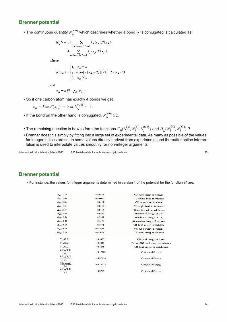
Brenner potential

• For instance, the values for integer arguments determined in version 1 of the potential for the function H are:


Brenner potential

• And for function F :

• In addition, Brenner also presented another parametrization of his potential.


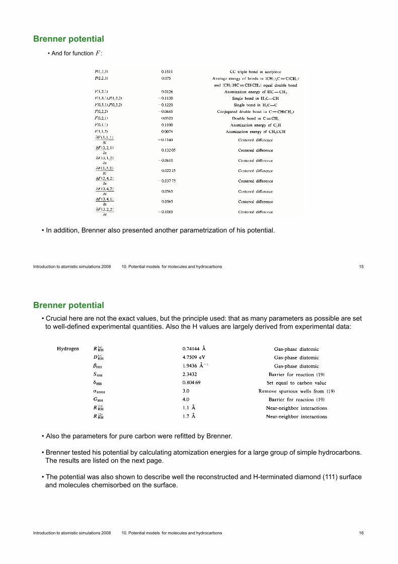
Brenner potential

• Crucial here are not the exact values, but the principle used: that as many parameters as possible are set

to well-defined experimental quantities. Also the H values are largely derived from experimental data:

• Also the parameters for pure carbon were refitted by Brenner.

• Brenner tested his potential by calculating atomization energies for a large group of simple hydrocarbons.

The results are listed on the next page.

• The potential was also shown to describe well the reconstructed and H-terminated diamond (111) surface

and molecules chemisorbed on the surface.


Brenner potential


Brenner potential


Brenner potential

• Later Murty and Atwater [Phys. Rev. B 51 (1991) 4889] have made a Si-H version of the Brenner poten-

tial, and Beardmore and Smith [Phil. Mag. A 74 (1996) 1439] a combined C-Si-H-version.

• Brenner himself has later added a torsional term to the potential, and at least two groups have added

long-range interactions (intermolecular interactions) into it: [Stuart et al., J. Chem. Phys. 112 (2000) 6472]

and [Che et al., Theor. Chem. Acc. 102 (1999) 346].


Brenner potential

• Example application: Beardmore and Smith examined in their paper how a fullerene C60 hits an Si sur-

face.

• Case I: 250 eV C60 ! virgin Si, incoming angle 80o i.e. the fullerene forms bonds with the surface and rotates along it

for a while (note the periodic boundary conditions).


Brenner potential

• But if the Si-surface is H-terminated (all dangling bonds are filled with a H) the behaviour changes:

Case II: 250 eV C60 ! H-terminated Si, 80o.

So the H protects the surface such that only a couple of bonds are formed with the surface, and the fuller-

ene bounces back almost impact, having only taken up one Si atom.


Brenner potential

• Case III: 250 eV C60 ! doubly H-terminated Si, 80o

• So now the protective H layer is so thick that there are no C-Si bonds formed at all, and the fullerene bounces back

intact.


Stuart potential

• Long range interactions are important also in graphite and in multiwalled carbon nanotubes (MWCNTs)

• Stuart et al. [J. Chem. Phys. 112 (2000) 6472] used the Lennard-Jones potential to

model the dispersion and intermolecular interaction:

Vij

LJr! " 4#

ij

$ij

r-------

% &' (

12 $ij

r-------

% &' (

6

–=

• However, LJ should be switched off when molecules approach

• Switching depends on interatomic distance [S tr

rij

! "! " ], bond order

[S tb

bij

! "! " ], and connectivity [Cij

]:

1

2

3

4

5

Connectivity: no LJ interaction among 1,2,3,4, LJ possible be-tween 1 and 5

Eb VR rij

! " BijVA rij

! " Eij

LJ+ +) *

j i+

,i

,=

Eij

LJS t

rrij

! "! "S tb

bij

! "! "Cij

Vij

LJrij

! " 1 S tr

rij

! "! "–) *Cij

Vij

LJrij

! "+=

• For C-C interaction $ij

3.40 Å= (graphite interlayer distance) - large neighbor lists (rcutoff 11 Å. )!


Stuart potential

• Example: Load transfer between shells in MWCNTs [M. Huhtala et al., Phys. Rev. B 70 (2004) 045404]

F

Intershell bond

No intershell bonds

Defect type Force (nN)

Single vacancy 0.08—0.4

Two vacancies 6.4—7.8

Intershell interstitial 4.9—6.3

Intershell dimer 3.8—7.3

molecular interaction models - helsinki

Documents