molecular dynamics for very large systems on … · .linearly and with number of cpus nearly...

— —< <

Molecular Dynamics for Very LargeSystems on Massively ParallelComputers: The MPSim Program

KIAN-TAT LIM,1 SHARON BRUNETT,2 MIHAIL IOTOV,1

RICHARD B. MCCLURG,1 NAGARAJAN VAIDEHI,1

SIDDHARTH DASGUPTA,1 STEPHEN TAYLOR,2 andWILLIAM A. GODDARD III1*1 ( )Materials and Process Simulation Center, Beckman Institute 139-74 , Division of Chemistry andChemical Engineering and 2Scalable Concurrent Programming Laboratory, California Institute ofTechnology, Pasadena, California 91125

Received 18 August 1995; accepted 12 June 1996

ABSTRACT

Ž .We describe the implementation of the cell multipole method CMM in aŽ . Ž .complete molecular dynamics MD simulation program MPSim for massively

parallel supercomputers. Tests are made of how the program scales with sizeŽ . Ž .linearly and with number of CPUs nearly linearly in applications involvingup to 107 particles and up to 500 CPUs. Applications include estimating thesurface tension of Ar and calculating the structure of rhinovirus 14 withoutrequiring icosahedral symmetry. Q 1997 by John Wiley & Sons, Inc.

Introduction

arge-scale systems with millions of atoms areL of great interest in many areas of chemistry,biochemistry, and materials science. Such systems

*Author to whom all correspondence should be addressed.E-mail [email protected]

This article includes Supplementary Material available fromthe authors upon request or via the Internet atftp.wiley.comrpublicrjournalsrjccrsuppmatr18r501 orhttp:rrwww.wiley.comrjcc

Ž .include viruses such as rhinovirus common coldand poliovirus that contain nearly one millionatoms1; starburst dendrimers2 where self-limitedgrowth of PAMAM may involve molecules withabout 250,000 atoms; and commercial polymerswhere typical molecular weights of 10 million dal-tons would lead to chains with millions of atoms.

Ž .Atomistic molecular dynamics MD simulationsof such large systems are important to provide theatomic detail needed to specify chemical proper-ties such as binding of a drug to a virus or me-chanical properties such as the modulus.3

( )Journal of Computational Chemistry, Vol. 18, No. 4, 501]521 1997Q 1997 by John Wiley & Sons CCC 0192-8651 / 97 / 040501-21

LIM ET AL.

In developing methodologies for routine appli-cations of MD to million-atom systems, it is impor-tant to retain accuracy while ensuring that thecomputational costs scale linearly with size.4, 5 The

Ž .key problems here are the long-range Coulomb QŽ .and van der Waals vdW interactions, collectively

Ž .referred to as nonbond NB interactions. Since theNB interactions include every pair of atoms, exact

Ž 2 .calculations require O N operations, where N isthe number of atoms, which is not feasible formillion-atom systems. The usual approach is totruncate the interactions at some cutoff distance.

Ž .This reduces the operation count to O N , butwith a significant decrease in accuracy, particu-larly for the Coulomb interactions.6

Fast multipole methods7 were developed toovercome these limitations. By treating the long-range interactions as multipole expansions oversuccessively larger regions, they avoid the inaccu-

Ž .racy of cutoffs while obtaining O N scaling withsize. They can be used for any inverse power-law

4 Ž .interaction potential including Coulomb 1rR ,Ž 2 . Ž 6.screened Coulomb 1rR , vdW dispersion 1rR ,

Ž 9 12 .and Pauli orthogonalization 1rR or 1rR . TheŽ .4cell multipole method CMM is a particularly

regular type of multipole method that is easilyimplemented on massively parallel computers. Inaddition, CMM has been extended to infinite sys-

Ž . 5tems while retaining the O N scaling. Previoustests4, 5, 8 of the CMM used single processor sys-tems. We report here the implementation9 of prac-

Ž .tical and accurate MD of massive million atomssystems on parallel processors. The current pro-gram is denoted as MPSim.

The next section of this article contains anoverview of CMM and the methods used to calcu-

Ž .late valence bonded interactions. The third sec-tion describes new results for large-scale simula-tions including rhinovirus and extrapolation oflarge argon clusters to the bulk limit. The imple-mentation of CMM on parallel computers is givenin the fourth section. The performance characteris-tics of the current code are presented in the fifthsection. Conclusions are in the final section.

Cell Multipole Method

Because it is not feasible to explicitly calculatethe interactions between all pairs of atoms in alarge system, we must find a way to approximatethe long-range region so as to decrease the costs toŽ .O N while maintaining sufficient accuracy. A tra-

ditional approach is to ignore interactions beyondsome cutoff. Unfortunately, this can lead to verylarge errors for Coulomb energies unless very longcutoffs are used.6

The key feature of multipole methods4, 5, 7 isthat long-range interactions are described usingmultipole fields representing large groups ofatoms. This drastically reduces the number ofcomputations, while including the effect of long-range terms. To maintain a given level of accuracywhile minimizing cost, the nearby interactions arerepresented more accurately than the weaker, moredistant interactions.

The long-range interaction portion of the simu-lation consists of computing and using these mul-tipole expansions, as is the case for other multipolemethods. The CMM is a particularly regular, easilyparallelizable multipole method that enables thistask to be performed efficiently. CMM consists offour parts:

1. Octree decomposition. The space occupied bythe system of interest is divided into a hierar-chical tree of cells so that long-range interac-tions can be treated using larger cells nearthe root of the tree, while short-range termsuse smaller cells near the leaves. The effect ofeach cell is represented by a multipole ex-pansion.

2. Multipole moment expansion. The multipolemoments are computed for each cell at eachlevel within the tree, starting from the leavesŽ .smallest cells and working toward the root

Ž .of the tree representing the entire system .

3. Far-field multipole potential expansion. The mul-tipole moments from step 2 are used to de-scribe the long-range fields due to the atomswithin a given cell. However, to calculate theforces on any one atom within a cell we needto sum the fields due to all other distant cellsin the system. These forces are described byexpanding the fields for the distant cells in aTaylor series expansion about the center ofthe cell where the forces will be calculated.These terms are summed to obtain the totalfar field as a single Taylor series expansion.These Taylor series coefficients are computedfrom the multipole moments from step 2,starting at the root of the tree and workingtowards the leaves. In carrying out this ex-pansion we exclude the effects of the atomsin neighbor cells since they will be includedexplicitly in the next step.

VOL. 18, NO. 4502

MPSIM PROGRAM

4. Atomic forces. Once the multipole potentialexpansions in step 3 are computed for eachleaf cell, the force on each atom is computedas a combination of the far field evaluated atthe atom location, the explicit nonbond inter-actions with nearby atoms, plus the short-

Ž .range valence forces. These forces are thenused in Newton’s equation to update veloci-ties and coordinates. Because the far fieldpotential changes slowly with time only step4 needs be carried out for each step of theMD.

OCTREE DECOMPOSITION

Ž .In CMM as used for finite cases , the system ofŽinterest is surrounded by a bounding box typically

a cube, but in general a parallelepiped specified by.three side lengths and three corner angles . This

box, the level 0 cell, is then subdivided into eightoctants by bisecting each side. The eight ‘‘child’’cells are then further subdivided into octants toform grandchildren cells, which are in turn subdi-vided in octants, etc., forming an octree decompo-sition of the original box. The maximum levelŽ .M of the tree is a parameter of the methodl e v eland is chosen to obtain the best combination ofspeed and accuracy. Increasing M increasesl e v elspeed but at the cost of decreased accuracy andincreased memory. The cells at this M arel e v elreferred to as the ‘‘leaf’’ cells.

Unlike adaptive multipole methods,10 in CMMthe octree decomposition is carried out to the samelevel across the entire system. This is appropriatefor applications to chemical, biological, and mate-rials systems because the variations of density are

Žseldom larger than an order of magnitude cells.with no atoms are ignored in the calculations .

This regularity simplifies determining the neigh-bors of any given cell and increases the number oftimesteps before it is necessary to rebuild the celltree.

NONBOND INTERACTIONS

We consider nonbond interactions of the form:

q qi j Ž .E s C aÝNB unit eRi ji)j

where e G 1 is an integer and the other terms aredefined in what follows. We use units of kcalrmol

˚for E and A for distances. Various special cases

are:

1. Coulomb interactions. Here, e s 1, the q areiparticle charges in electron units, and:

332.0637Ž .C s bunit «0

Žwhere « is the static dielectric constant we0.use « s 1 for a vacuum .0

2. Shielded Coulomb interactions. For systems inŽ .which a polar solvent particularly water is

treated implicitly, a common approach forŽ .Coulomb interactions is to use eq. a with

e s 2.3. van der Waals dispersion. The interaction con-

stants can be written as:

C C'C ii j ji j Ž .E s s cÝ Ýdi s p 6 6R Ri j i ji)j i)j

where the standard combination rule:

Ž .C s C C d'i j i i j j

Ž .is assumed. In eq. a we use e s 6, q s C ,'i i iand C s 1.unit

( )4. van der Waals repulsion Pauli orthogonality .The repulsive short-range nonbond interac-tions are often described as:

A A'A ii j ji j Ž .E s s eÝ Ýr e p 12 12R Ri j i ji)j i)j

or:yB i j R i j Ž .E s A e fÝr e p i j

i)j

Ž . Ž .Using eq. e with eq. c leads to theŽ .Lennard]Jones 12-6 potential, whereas eq. f

Ž .with eq. c leads to the exponential-6 orŽ .Buckingham potential. Term e can be

treated using CMM. However, these termsw Ž . Ž .xusing e or f fall off sufficiently fast withR that long-range calculations are not impor-tant. Thus, we treat case 4 using truncation,rather than multipoles.

MULTIPOLE EXPANSIONS

The potential far from a collection of chargescan be written as the multipole expansion:

ªye yey2Ž . Ž .V R s qR q m ? R R1 yey4Ž . Ž .q R ? Q ? R R q ??? g2

JOURNAL OF COMPUTATIONAL CHEMISTRY 503

LIM ET AL.

ªwhere q, u, Q describe the total charge, dipolemoment, quadrupole moment, etc., for the collec-

Ž .tion of charges. The maximum level M ofp o l eŽ .multipole expansion to be used in eq. g is a

parameter to be specified in CMM. Ding et al.4, 5

considered truncating at the quadrupole termsŽ . Ž .M s 2 as in eq. g or keeping the next levelp o l eŽ .or octopole, M s 3 and found that M s 2p o l e p o l eleads to sufficient accuracy at reasonable costs.Increasing M increases the accuracy at the costp o l eof extra computation time.

The moments within a cell are calculated as:

q s qÝcel l at omatoms

m s eR qÝcel l , a a at omatoms

Ž .1

2Ž .Q s e e q 2 R R y eR d qÝcel l , a b a b a b at omatoms

where q, m , and Q are the charge, dipole, anda a b

quadrupole moments, respectively; R s R ya at om , aª ªR ; R is the position of the atom; Rcent er , a at om cent eris the center of the expansion; the energy compo-nent is proportional to Rye ; and a s x, y, z.

The centers of the multipole expansions can bechosen in several different ways. The simplestchoice is to use the geometric centers of the cells.However, if the atoms within a cell are not dis-

Žtributed evenly, expanding about the centroid or.average of the atom locations:

1ª ª Ž .R s R 2Ýcent r o id at omn

Ž .where n is the number of atoms in the cellproduces improved accuracy for a given level ofmultipole expansion. The centroids are computed

Žhierarchically using the existing cell tree the cen-troid of a higher level cell is equal to the weightedaverage of the centroids of its children, where theweights are the number of atoms in each child

.cell . The increased accuracy from the centroidformulation allows the use of more highly trun-cated expansions than would otherwise be re-quired. The ‘‘Accuracy’’ subsection provides moredetails.

Charge-weighted and mass-weighted averageswere tried, but these alternative centers were notfound to significantly improve the accuracy.

Once the leaf cell multipole moments have beencomputed, the expansions may be translated to the

Ž .centers of the next larger ‘‘parent’’ cells andcombined to obtain the multipole moments repre-

senting the parent cell:

q s qÝp ar ent chi l dchildren

w xm s m q eR qÝp ar ent , a chi l d , a a chi l dchildren

Ž .Q s Q q e q 2Ýp ar ent , a b chi l d , a bchildren

Ž .3

Ž .= R m q R ma chi l d , a b chi l d , b

Ž .qe e q 2 R R qa b chi l d

ª ª 2y 2 R ? m q eR q dž /chi l d a b

This process continues through the tree until theŽ .root level 0 cell is reached. At this point, every

cell in the system has associated with it a multi-pole expansion representing the field due to all ofthe atoms contained within the cell.

MULTIPOLE FIELD EXPANSIONS

To compute energies and forces on a given atomwithin the system, we need to obtain the field dueto all of the other atoms in the system. This isbroken into two components: the near-field interac-tion due to all of the atoms in the same cell or the26 neighboring cells, and the far-field interactiondue to all of the rest of the atoms. In CMM, thenear-field interactions are evaluated explicitly toensure high accuracy while the far-field interac-tions are evaluated using effective fields.

The far-field potentials to be applied to anyatom in a given cell are combined into a Taylorseries expansion about the center of the cell. Thispotential is then used to calculate the energy atany point within the cell. The coefficients of thisexpansion are determined from the multipole ex-pansions computed in the previous subsection.

The Taylor series expansion of the farfield iswritten as4:

ªŽ . Ž .V R s V q V R q V R R q ??? 4Ý Ý0 a a a b a ba ab

ª ª ªwhere R s R y R and V , V , and Vat om cent er 0 a a b

are the expansion coefficients. The centers used forthe multipole field expansion are the same as thoseused for the multipole moment expansion.

Ž .Given the multipole potential Taylor expan-sion for a cell’s parent, the remaining contributionsneeded to obtain a cell’s far-field expansion are:

( )i the fields from the 8 children of each of theparent’s 26 neighbors, plus

VOL. 18, NO. 4504

MPSIM PROGRAM

( )ii the fields from the other 7 children of theparent, minus

( )iii the fields from the cell itself and its 26immediate neighbors at its level.

Ž .This leads to 27 cells parent and its neighborsŽ . Žtimes 8 children per cell minus 27 cells cell and

.its neighbors , or 189 cells. All children of the sameparent can be omitted because they are immediateneighbors of each other. Thus, to the parent’s far-field expansion we add the fields from the 189

Ž .parent cell’s neighbors’ children PNCs to formŽthe far field of the child understanding that the

other immediate neighbors of the cell in question.are excluded .

To start this process, note that all cells at level 1Ž .the first set of eight child cells are immediateneighbors of each other, and thus there is no far-field contribution from the parent or the PNCs ofthese cells.

By induction, we can continue generating Tay-lor expansions all the way to the leaf cells, atwhich point every cell has a Taylor expansionrepresenting the far field within the cell.

We define the following useful terms:

ª ª ª Ž .R s R y R 5cent er , P NC cent er , cel l

Ž .m s m R 6Ý a aa

Ž .Q s Q R R 7Ý a b a bab

The contributions from each PNC to the expan-sion coefficients are then:

1ye yey2 yey4 Ž .V s R q y R m q R Q 80 2

yey2 yey2 y2Ž .V s e qR R y R e q 2 R R m y ma a a a

1yey4 y2Ž . Ž .q R e q 4 R R Q y Q R 9Ýa a b b2 b

1yey2 y2 2Ž .V s e qR e q 2 R R y 1a a a2

yey4 Ž .q R e q 2 m Ra a

1yey4 y2 2Ž . Ž .y e q 2 mR e q 4 R R y 1a2

1yey4q R Qa a2

1yey6 y2 2Ž . Ž .q e q 4 QR e q 6 R R y 1a4

Ž . yey6 Ž .y e q 4 R R Q R 10Ýa a b bb

Ž . yey4V s e e q 2 qR R Ra b a b

Ž . yey4q e q 2 Ry2Ž .= m R q m R y e q 4 R mR Ra b b a a b

q Ryey4Qa b

Ž . yey6 Ž .y e q 4 R Q R R q Q R RÝ ag b g gb a gg

1yey8Ž .Ž . Ž .q e q 4 e q 6 QR R R 11a b2

where the q, m, and Q multipole expansion coeffi-cients are those of the PNC.

The contributions from the parent cell’s Taylorseries coefficients to one of its child cells’ coeffi-cients are:

Ž .V s V q V R q V R R 12Ý Ýchi l d , 0 0 a a a b a ba ab

Ž .V s V q V R q V R 13Ýchi l d , a a a a a a b bb

Ž .V s V 14chi l d , a b a b

ª ª ªwhere R s R y R here, and thecent er , chi l d cent er , p ar entV coefficients on the right are from the parent cell.

FAR-FIELD EVALUATION AND NEAR-FIELDCOMPUTATION

Once the cell Taylor expansions have been de-termined, computing the interaction energy andforce due to the far-field at each atom is simply amatter of evaluating the Taylor series at the atom’s

w Ž .xposition given by eq. 4 and calculating the in-teraction of the field and the atomic charge.

Because the far field changes much more slowlythan the near field, it is feasible to perform thefar-field calculation at intervals of every 5 to 10timesteps. The centers and coefficients of the Tay-lor series expansions representing the far field arekept constant during the interval.

The remaining near-field interactions betweenan atom and the other atoms in the same cell andin neighboring cells are computed explicitly, usingthe appropriate charge-charge interaction equa-

Ž .tions Coulomb or van der Waals .

VALENCE FORCE FIELD CODE

Ž .The valence force field FF consists of interac-tions defined in terms of the bonds and anglesbetween atoms in a molecule. These terms are


LIM ET AL.

used to parameterize the quantum-mechanical ef-fects due to stretching the chemical bonds andbending the angles.

Among the terms we use are:

( )a Bond stretch: harmonic or Morse potentials:

21 Ž . Ž .E s K R y R 15ab b e2

or:

2yaŽRyR .ew x Ž .E s D e y 1 15bb e

where R is the equilibrium bond length, K ise bthe force constant, D is the bond energy, andea s K r2 D is the Morse scaling parameter.' b e

( )b Angle bend: harmonic or harmonic-cosine po-tentials:

21 Ž . Ž .E s K u y u 16aa u e2

or

21 Ž . Ž .E s C cos u y cos u 16ba u e2

where u is the equilibrium angle, K the forcee u

constant, and C s K rsin2 u .u u e

( )c Torsion: cosine expansions:

121Ž . Ž .E s V q V )cos nf 17Ýf 0 n2 ns1

where V is the barrier for the nth-fold rota-ntion.

( )d Inversion: harmonic-cosine potentials:

21 Ž . Ž .E s K cos c y cos c 18c c e2

where c is the equilibrium angle and K thee c

force constant.( )e Cross terms: combinations of the above terms

used to improve the accuracy of vibrationalfrequencies: For two atoms I and K bonded toJ, we have:

Eb ond — an g l e

Ž .Ž e .s K cos u y cos u R y Rr1u e 1 1

Ž .Ž e . Ž .q K cos u y cos u R y R 19ar 2u e 2 2

Ž e .Ž e . Ž .E s K R y R R y R 19bb ond — b ond r r 1 1 2 2

where R s R and R s R and the Ks are1 I J 2 JKforce constants. For atoms in the dihedral I—

J—K—L, we include:

Ean g l e — an g l e

Ž .Ž e .s K f f cos u y cos uaa x I JK I JK

Ž e . Ž .= cos u y cos u 19cJK L JK L

to couple the angle I—J—K with the angleŽ .J—K—L. The f f factor depends on the di-x

Ž .hedral f and has the form f f sI — J — K — L 7Ž . Ž . Ž .1 y 2 cos f r3, f f s cos f, or f f s 1.1 0

Important features of the above valence FF termsare:

1. A variety of functional forms is associatedwith each type of interaction to allow anaccurate description of the FF.

2. The functions depend on the coordinates oftwo, three, or four atoms. The input file onlyprovides a list of bonds between atomsŽequivalent to edges between nodes in a

.graph . The program deduces the three- andfour-body interactions from the two-bodyconnectivities.

3. The functional forms and the constants ineach function depend on the types of theatoms participating in each interaction. Thesetypes typically involve the element or atomicnumber of the atom plus information abouthybridization or oxidation state of the atom.

All of these points must be taken into account toproduce a useful, general MD code, but they alsomake parallelization of the valence FF computa-tion more difficult. We therefore describe some ofthe techniques used to overcome this problem.

Each term is assigned to exactly one of theatoms participating in the interaction. To minimizethe distance between the responsible atom and theother atoms in the interaction, the central atom ofeach angle term and the center atom of each inver-sion term is designated as the responsible atom.For torsions, one of the two middle atoms is used.

For each term for which an atom is responsible,Ž .the type of term anglertorsionrinversion , the

numbers of the other atoms participating in theinteraction, and an index into an array of struc-tures for that term type defining the functionalform and constants for the interaction are stored ina list associated with that atom. Functions areprovided to iterate through all interactions of agiven type.

VOL. 18, NO. 4506

MPSIM PROGRAM

Cross-terms are not stored as separate interac-tions; rather, they modify the functional forms ofthe relevant three- or four-body interactions.

Bonds are treated slightly differently, as theirinformation is also needed to maintain the molecu-lar connectivity. For each atom, the other atomsbonded to it and the index to the array of bondfunctionrconstant structures are stored in a sepa-rate list associated with that atom.

These lists are computed only once because thebonding network does not change.

Each CPU can compute all the interactions forthe atoms residing on that CPU provided that ithas access to the atomic coordinates for each atomparticipating in any such interaction. In physicalsystems, all atoms participating in an interactionmust be close in space, and we assume that allatoms participating in any given valence interac-tion are either in the same leaf cell or in a neigh-boring leaf cell. With this assumption all atomiccoordinates for all atoms of interest to the valenceinteractions will have already been communicatedto the cell during the near-field computation of theCMM. They are merely saved until the valenceinteractions have been computed. On machinesthat provide a shared memory programmingmodel, this assumption need not be embedded inthe code, but it still serves to increase performanceby ensuring that needed data will be in localmemory rather than on a remote node.

Each computation produces a force vector foreach atom that must be added to all other forcecomponents for that atom. For the computed par-tial forces to be added into each atom’s forcevector, we accumulate these forces locally on eachnode both for the local atoms assigned to the celland for the nonlocal atoms in neighboring leafcells that were involved with a valence term as-signed to the cell. Then, after all the valence FFcalculations have been completed, we send partialforces of nonlocal atoms back to the node fromwhich the atomic coordinates were obtained. Thatnode then adds the incoming partial forces into thelocal atom force vectors.

In the current implementation, each atom par-ticipating in a bond interaction is responsible forcomputing half of the energy contribution and thepartial force exerted on itself by the bond. Thus,partial bond forces need not be communicated.Given that partial forces for the other terms arebeing communicated, this inefficiency will be elim-inated in the future.

On machines with a message-passing architec-ture, each node creates a list of all remote cells

required to perform its own calculations. It thensends a request to the appropriate nodes asking forthat remote cellratom information.

As the calculation progresses, the force compo-nents on remote atoms are updated. When theseupdates are complete, each CPU goes through itslist of remote atom data, bundles the updatedinformation, and sends it back to the CPU owningthe remote atoms. Each CPU then receives updatesmade to its local atoms and adjusts the force vec-tors appropriately. Subsequent calculations involv-ing an atom’s force vectors then proceed.

Three other terms related to the valence FF arecomputed rather differently:

1. Nonbond exclusions. Because the valence FFusually implicitly includes any contributionsfrom nonbonded interactions between atoms

Žthat are bonded to each other 1]2 interac-. Žtions or bonded to a common atom 1]3

.interactions , the corresponding nonbondedenergies and forces included in the CMM

Žmust be excluded from the final result. Inaddition, for the AMBER FF,11 the 1]4 terms

.are also scaled, requiring similar corrections.This can be implemented in two ways:

( )i avoid the computation of these non-bonded interactions during the inner loopof the near-field calculation in CMM; or

( )ii subtract out their effects as a separatestep.

Ž .Method i reduces floating-point operations,but at the cost of many memory references to

Ž .do table look-ups. Method ii computes someinteractions twice and increases errors due tosubtraction of large numbers, but it avoidsconditional branches and uncached memoryaccesses in performance-critical code. We use

Ž .method ii in the current implementation.

2. Hydrogen bonds. For the nonbond interactionbetween a hydrogen atom and a hydrogenbond acceptor, some FFs use a modifiedfunctional form in place of the usual 6]12vdW term. For example, the AMBER FF11

uses:

Ž . y12 y10 Ž .E R s AR y BR 20i j

where R is the distance between the acceptorŽ .atom N, O, F, S, Cl and the hydrogen atom

of the donor. These are implemented as a


LIM ET AL.

modified nonbond exclusion, in which theoriginal energy and force is subtracted whilethe new term is added.

3. Off-diagonal nonbonds. Explicit in the use ofCMM is the geometric mean combination

Ž . Ž . Ž .rule in eq. d , which is used in eq. c and f .This can be written as follows:

Ž . Ž . Ž . Ž .D s D ? D 21a'i j j j0 0 0i i

Ž . Ž . Ž . Ž .R s R ? R 21b'i j j j0 0 0i i

Some FFs prefer the use of an arithmeticmean:

Ž . Ž . Ž . Ž .D s D ? D 22a'i j j j0 0 0i i

1Ž . Ž . Ž . Ž .R s R q R 22bi j j j0 0 02 i i

Ž .Sometimes particularly for hydrogen bondsit is necessary to use a special, different func-tional form to express the van der Waalscomponent of the nonbond energy betweentwo types of atoms.

Ž .Our implementation allows the D and0 i jŽ . Ž .R to be different than in eq. d or eq.0 i jŽ .21 for specific pairs of atoms.

As for the valence FF terms, the atoms partici-pating in nonbond exclusions are determined atinitialization. Each atom has a list of other atomsfor which the exclusions should be computed.

ŽOff-diagonal nonbonds and their special case,.AMBER-type hydrogen bonds cannot be prede-

fined by an unchanging list. Instead, we generatethis list each time the CMM far-field is updated.We again assume that only interactions with atomsin nearest-neighbor leaf cells are of interest. Allpairs of atoms within a leaf cell or in adjacent leafcells are tested to see if they have both a hydro-gen-bond donor and acceptor or have atom typesfor which an off-diagonal nonbond has been de-fined. Those pairs that qualify are then added tothe list.

At each timestep, the pairs of atoms in theexclusion lists have the CMM-calculated interac-tion subtracted. For off-diagonal nonbond interac-tions, a new energy term is then calculated andadded.

All of the above terms are sufficiently general toimplement the functional forms and constants usedin standard molecular mechanics force-fields suchas AMBER11 and DREIDING II.12

INTEGRATION

In the current implementation, the dynamicsstep in the simulation uses either a simple Verlet

Ž .13integrator for microcanonical dynamics or aŽNose]Hoover constant-temperature integrator for´

. 14canonical dynamics . In either case, the atomicforces are integrated to generate the new atomicvelocities, which are in turn integrated to give newatomic positions. The equations of motion are asfollows:

Verlet:

ªfnª ª Ž .1 1v s v q D t 23nq ny2 2 m

ª ª ª Ž .1x s x q v D t 24nq1 n nq 2

Nose]Hoover:´ª

1 f D tnª ª Ž .1v s v q 25n ny 2D t ž /m 21 q zn 2

ªD t f D tnª ª Ž .1v s v 1 y z q 26nq n n2 ž /2 m 2

ª ª ª Ž .1x s x q v D t 27nq1 n nq 2

D tŽ .1s s s qz 28n ny n2 2

D tŽ .1s s s q z 29nq n n2 2

1T1 nq 2 Ž .z s z q y 1 D t 30nq1 n 2 ž /Tt b aths

3N2 2 Ž .KE s k T t z 31b ath B b ath s n2

Ž . Ž .PE s 3N q 1 k T s 32b ath B b ath n

m v2 KEi i , n nT s sÝn 3Ž . Ž .3Nk NkB 2i

ª ª ªf , v, x, and m are the atomic forces, velocities,coordinates, and mass, respectively. The subscripts

1n, n q , and n q 1 denote increasing timesteps. z2

is the Nose]Hoover friction variable responsible´for transferring heat from the system to the bath orvice versa, s is its integral, and t is the timesconstant associated with the heat transfer. The

1instantaneous kinetic energy, KE , is written innq 2

1terms of a temperature, T ; this must be evalu-nq 2

ated at the half-step because it is used to compute˙ 1z , which is needed to obtain z . T is thenq nq1 b ath2

VOL. 18, NO. 4508

MPSIM PROGRAM

Ž .constant bath temperature. N is the number ofatoms in the system.

The MPSim program also allows for periodicŽ . 5systems RCMM . The applications here discuss

only the finite case.

Applications

ARGON CLUSTER

We previously studied15 the properties of smallclusters as a function of size and developed anapproach for extracting quantities which could beused to predict the free energy or arbitrarily largeclusters and for the infinite crystal. These calcula-tions were based on MacKay clusters with up to561 atoms.

It is well known from both experiment andŽ 16 17theory that van der Waals complexes Ar, CH ,4

.etc. lead to icosahedral clusters with particularstabilities for certain magic numbers correspondingto Mackay icosahedral structures,18 whereas the

Ž .bulk crystal leads to a face-centered cubic fccstructure. For Ar, the Mackay icosahedral structureis most stable for up to about 1600 atoms, the bulkfcc structure is most stable above about 105 atoms,and other structures are stable in the intermediatesize range.19 The magic number Mackay icosahe-dral structures are composed of concentric filledshells surrounding a central atom.

Using MPSim we have now explicitly calculatedŽstructures for very large Mackay clusters up to

7 .10 atoms and for large fcc clusters. These resultsare used to scale the properties to infinite systems.These are among the largest simulations of

Ž .Lennard]Jones LJ systems. Lomdahl and co-workers20 were the first to study multimillion-particle systems. They simulated a two-million LJparticle system at 0 K in two dimensions as itfailed under one-dimensional strain.20

We use a simple LJ 12-6 potential with equilib-˚rium separation R s 3.82198 A and well depthe

D s 0.23725 kcalrmol. These were determined toe˚Ž .fit the structure a s 5.31 A and cohesive energy

Ž .E s 1.848 kcalrmol of Ar crystal at 0 K.cohTo test the accuracy of MPSim, we quenched a

Mackay icosahedral cluster and a spherical fcccluster, both with 10,179 atoms. With a cell occu-

Žpancy of 10,179 i.e., with all atoms in the same.cell , we calculated a binding energy of 80219.2) De

for Mackay and 80243.3) D for FCC. These resultseagree, to all six significant figures, with the litera-ture values.21

The accuracy of the method as a function ofaverage occupany and CMM level is depicted inFigure 1. Figure 1d shows that to obtain a struc-

˚ture with an rms coordinate error of 0.05 A re-quires an accuracy in the rms force error of 0.01

˚Ž .kcalrmol rA. Figure 1c illustrates that, for 100,000atoms this accuracy is obtained with level 5 whichFigure 1a shows to have about 10 particles per cell.

FCC Structures

Because the optimal structure for large clustersis likely fcc or nearly fcc, we chose to quenchmagic number spherical fcc clusters to determinetheir maximum binding energy.

Table I summarizes the minimization parame-ters, maximum binding energy, and rms force foreach of the clusters studied. The fcc clusters have

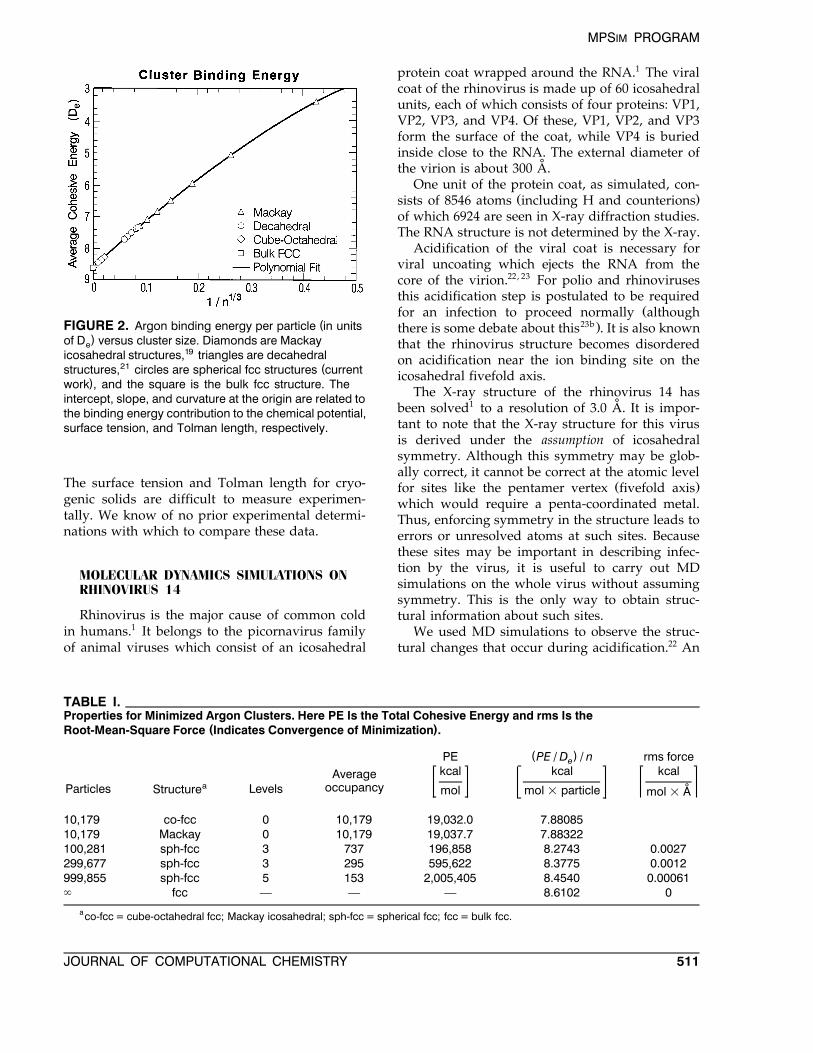
Ž .binding energies per particle Ern which are con-sistent with known values for smaller clusters andthe bulk structure. To estimate the limits for an

Ž . y1r3infinite crystal we plot Ern versus n inFigure 2. We found that going beyond ny4r3 in thepolynomial expansion leads to insignificant im-provement in the rms error. Thus we truncated theexpansion at the fifth-order term.

PEy1r3 y2r3 y1 y4r3s a q bn q cn q dn q en

mDe

Ž .33

The fitting parameters are a s y8.60990 "0.00041, b s q15.74416 " 0.037, c s y11.89436 "0.77, d s q17.19378 " 1.1, and e s y20.38740 "1.5. This fit is somewhat less precise than that ofXie et al.19 when applied to small clusters, but ismore accurate for extrapolation to large clusters.We have determined the binding energy contribu-tion to the chemical potential, surface energy, and

Ž .Tolman length see Fig. 2 . As discussed else-where:15

( )i the intercept a gives the bulk chemicalpotential, m;

( ) y1r3ii the slope b at n s 0 is proportional tothe surface tension, s ; and

( )iii the ratio crb of the curvature to the slopeat ny1r3 s 0 is proportional to the Tolmanlength, d .

We use our previous estimate15 for the zero-point energy and limit our discussion to 0 K tohighlight the current results without extraneouscomplications.


LIM ET AL.

( )FIGURE 1. Dependence of the accuracy of CMM on the octet level for Ar . Empty cells are not counted in100,000˚computing occupancy; thus the lowest possible occupancy is one. A cube of side = 240 A was placed around the

˚( ) ( ) ( ) ( )Ar cluster diameter = 190 A . a The average occupancy vs. level. b The rms force error vs. average100,000( ) ( )occupancy. c The rms force error vs. level. d The rms force error vs. error in minimized structure.

Ž . y1r3The parameters from eq. 33 , at n s 0, to-gether with our previously published zero-pointenergy estimate,15 allow us to estimate the chemi-

Ž . Ž .cal potential m , surface tension s , and TolmanŽ .length d at 0 K.

Ž .m s D = a q 30.861hn 34e char

1r3 2r3Ž . w Ž . Ž . xs s D = b y 34.413hn 4p 3ve char

Ž .35

1r31 c 3vŽ .d s yD = q 10.594hn 36e charž / ž /2 b 4p

Here, v is the molecular volume at 0 K and hncharis a characteristic zero-point energy.15 We expectthese estimates to be more accurate than previous

efforts because all three properties are dominatedŽby the binding energy contribution as opposed to.the zero-point energy contribution and our esti-

mates benefit from minimizations of very largeŽ .clusters see Table I and Fig. 2 . This illustrates one

use of massive molecular dynamics in probing theasymptotic approach of cluster properties towardthe bulk limit.

˚3ŽUsing the values for argon v s 37.456 A ratom,.hn s 6.181 calrmol gives the following esti-char

mates:

m0 K s y1.852 kcalrmolA r

s 0 K s 45.2 dynrcmA r

0 K ˚d s 0.81 AA r

VOL. 18, NO. 4510

MPSIM PROGRAM

(FIGURE 2. Argon binding energy per particle in units)of D versus cluster size. Diamonds are Mackaye

icosahedral structures,19 triangles are decahedral21 (structures, circles are spherical fcc structures current

)work , and the square is the bulk fcc structure. Theintercept, slope, and curvature at the origin are related tothe binding energy contribution to the chemical potential,surface tension, and Tolman length, respectively.

The surface tension and Tolman length for cryo-genic solids are difficult to measure experimen-tally. We know of no prior experimental determi-nations with which to compare these data.

MOLECULAR DYNAMICS SIMULATIONS ONRHINOVIRUS 14

Rhinovirus is the major cause of common coldin humans.1 It belongs to the picornavirus familyof animal viruses which consist of an icosahedral

protein coat wrapped around the RNA.1 The viralcoat of the rhinovirus is made up of 60 icosahedralunits, each of which consists of four proteins: VP1,VP2, VP3, and VP4. Of these, VP1, VP2, and VP3form the surface of the coat, while VP4 is buriedinside close to the RNA. The external diameter of

˚the virion is about 300 A.One unit of the protein coat, as simulated, con-

Ž .sists of 8546 atoms including H and counterionsof which 6924 are seen in X-ray diffraction studies.The RNA structure is not determined by the X-ray.

Acidification of the viral coat is necessary forviral uncoating which ejects the RNA from thecore of the virion.22, 23 For polio and rhinovirusesthis acidification step is postulated to be required

Žfor an infection to proceed normally although23b.there is some debate about this . It is also known

that the rhinovirus structure becomes disorderedon acidification near the ion binding site on theicosahedral fivefold axis.

The X-ray structure of the rhinovirus 14 has1 ˚been solved to a resolution of 3.0 A. It is impor-

tant to note that the X-ray structure for this virusis derived under the assumption of icosahedralsymmetry. Although this symmetry may be glob-ally correct, it cannot be correct at the atomic level

Ž .for sites like the pentamer vertex fivefold axiswhich would require a penta-coordinated metal.Thus, enforcing symmetry in the structure leads toerrors or unresolved atoms at such sites. Becausethese sites may be important in describing infec-tion by the virus, it is useful to carry out MDsimulations on the whole virus without assumingsymmetry. This is the only way to obtain struc-tural information about such sites.

We used MD simulations to observe the struc-tural changes that occur during acidification.22 An

TABLE I.Properties for Minimized Argon Clusters. Here PE Is the Total Cohesive Energy and rms Is the

( )Root-Mean-Square Force Indicates Convergence of Minimization .

( )PE PE / D / n rms forceekcal kcal kcalAverage

a occupancyParticles LevelsStructure ˚mol mol = particle mol = A

10,179 co-fcc 0 10,179 19,032.0 7.8808510,179 Mackay 0 10,179 19,037.7 7.88322100,281 sph-fcc 3 737 196,858 8.2743 0.0027299,677 sph-fcc 3 295 595,622 8.3775 0.0012999,855 sph-fcc 5 153 2,005,405 8.4540 0.00061` fcc — — — 8.6102 0

aco-fcc = cube-octahedral fcc; Mackay icosahedral; sph-fcc = spherical fcc; fcc = bulk fcc.


LIM ET AL.

understanding of these structural changes shouldbe useful in designing new antiviral agents toinhibit uncoating of the viral coat of the rhi-novirus. These simulations were carried out using

Ž .MPSim. Rhinovirus 14 Fig. 3 requires both va-lence and nonbond forces in the simulation.

To allow for hydrogen bonding, hydrogens wereadded where appropriate to oxygen, nitrogen, andsulfur atoms of the X-ray structure of the asym-metric unit. Due to the acidic and basic residuesthere was a net charge of y5 on each asymmetricunit. In water, such exposed atoms lead to solva-tion by water dipoles and free ions near the charge.In our calculations we simulated this solvation by

Ž q y.adding counterions Na and Cl close to theŽ .side chains of the acidic Asp, Glu and basic

Ž .residues Lys, Arg . Not every charged residuerequires a counterion, because many are involvedin salt bridges. We eliminated such paired sidechains by examining all pairwise distances be-tween the central atoms of oppositely charge sidechains. These atoms are C in aspartic acid, C ind d

glutamic acid, C in arginine, and N in lysine.d d˚Pairs less than 10 A apart were considered to

stabilize one another, and were not given counter-charges, since these pairs may be involved in saltbridges. This automated procedure of addingcounterions resulted in adding 1500 counterions to

Ž q y.the whole virus 900 Na and 600 Cl .The X-ray structure is unresolved for the first 28

residues of the VP4 protein which is buried insideclose to the RNA. The RNA is also not included in

FIGURE 3. The minimized structure of rhinovirus 14 starting from the X-ray structure 4RHV in the Brookhaven( )database. The shades of red show the pentameric site formed by the VP1 subunit. VP2 is in green or shades of green

( )and VP3 is in blue or shades of blue . VP4 atoms are buried inside and some of them are seen in yellow.

VOL. 18, NO. 4512

MPSIM PROGRAM

the current calculations, because no structure isŽavailable for it it does not have icosahedral sym-

.metry and hence is invisible in the X-ray .The asymmetric unit thus has 8546 atoms which

includes the heteroatom hydrogens, the counteri-ons placed to neutralize the charges, and the crys-tallographic waters. The full viral coat of rhi-novirus 14 has 512,760 atoms. Explicit waters inthe calculation would improve the accuracy butwere excluded. This omission is compensated par-tially in two ways:

1. By using a distance-dependent dielectric tomimic the charge-shielding capacity of waterbetween charges i and j:

q q q qi j i jŽ . Ž .E q , q s s 36i j 2« r « re f f i j i j

2. By using counterions to balance charges onthe side chains of residues.

The whole virus structure, along with the crys-tallographic waters and the counterions, was mini-mized using the AMBER FF.11 A steepest-descent

Ž .method dynamics at 0 K was used. The timestepwas set to 0.75 fs since the lone pairs on the sulfursare included explicitly. The FF parameters used forthe counterions Naq and Cly are those corre-sponding to the hydrated ions.24 Hydrated ionswould attenuate the electrostatic interaction be-tween the ions and the charged groups in the sidechains. The rms force on the final minimized struc-

˚ture is 0.2 kcalrmolrA. The radius of gyration of˚the starting structure was 133.49 A and remains

Ž .unchanged 0.001% during the minimization. Therms difference in coordinates between the starting

˚structure and the minimized structure is 0.268 A.This value was calculated considering only the

Žatoms in the viral coat excluding the crystallo-.graphic waters and the counterions .

The minimized structure was then equilibratedŽat 300 K using Nose]Hoover constant tempera-´

.ture dynamics. The Nose time constant was cho-´sen to be t s 7.5 fs which is ten times25 theno setimestep used for integration. The MD was donefor 15 ps at 300 K until equilibrium was reached.The temperature of the system reached an equilib-rium after 5 ps of dynamics to an average value of295.99 K. We observe that the equilibrated virusstructure does not disassemble in spite of the RNAbeing absent. Further studies on the effect of low-ering the pH are ongoing.

Implementation

We implemented the CMM for message-passingparallel multicomputers. Unlike some other paral-lel multipole method implementations,26 this is athree-dimensional, fully distributed code, allowingthe solution of large-scale problems that would notfit in the memory of a single processor.

The pseudocode for the algorithm used is pre-sented in Appendix A of the Supplementary Mate-

Žrial see footnote on p. 501; also available at.http:rrwww.wag.caltech.gov .

MESSAGE TYPES

Five types of messages form the heart of theCMM algorithm:

1. Cell center sent from a child cell to its parentcell.

2. Multipole moments sent from a child cell toits parent cell.

3. Multiple moments sent from a cell to itsPNCs.

Ž .4. Multipole far-field Taylor series coefficientssent from a parent cell to its children.

5. Atoms sent from a leaf cell to its neighbors.

The first four are used to compute the far-field andoccur only every N timesteps; the last type ofu p dat emessage must be executed at every timestep.

The cell centers need to be sent through the treebefore the multiples because each parent cell mustdetermine the location of its center before process-ing incoming multipoles from its children.

Additional messages are used for initialization,synchronization, flow control, and atom reassign-ment.

ACTIVE MESSAGES

An active message model was used for thedevelopment of the code. In this model, receptionof a message triggers the execution of a functionspecified in the message with the message con-tents passed as an argument or arguments to thefunction.27 This model allows low-latency commu-nications by avoiding copying. It also leads to anatural, asynchronous, multithreaded style of pro-gramming. We believe that the advantages of theactive message model will make it the preferred


LIM ET AL.

programming model for future generations ofmulticomputers.

Currently, the active message model is the pre-ferred model for programming experimental finegrain parallel processing hardware such as theMIT J- and M-machines,28 which are among thetargeted platforms for this code.

As an example, the second type of messagefrom the previous section, involving the communi-cation of multipoles from a cell to its parent, isimplemented through an active message of thetype CHILD, with the destination CPU, destina-

Ž .tion parent cell, and sending cell’s multipoles asarguments. When such a message is received onthe destination CPU, it triggers the invocation ofthe child() routine given in the pseudocodeŽ .Appendix A which parses the arguments, obtainsthe appropriate destination cell, and calls a purelycomputational routine to combine the child’s mul-tipoles with the parent’s.

Although active messages have not been exten-sively used on traditional multicomputers such asIntel’s Delta and Paragon,29 we have found thatrefinements can be added to improve performanceon such architectures, primarily by gathering to-gether multiple small messages into a few largemessages. This buffering significantly reducesper-byte overhead.

Because the fundamental messaging primitiveshave no flow control, we implemented a flowcontrol system on top of the active messages. Eachprocessor is allowed to send a certain number of

Ž .messages a window to each other processor inthe system. When the window is full, it must waituntil it has received acknowledgments beforesending more messages. Keeping the windows ona per-processor basis allows more messages to be

Ž .outstanding not acknowledged than if a singlewindow were used on each processor. This in turnreduces the amount of nonproductive busy-waiting on each processor.

The acknowledgment can often be packed withmessage data needed to continue the calculation.In addition, we could optimize further by sendingbuffered messages taking into account the size ofthe system message buffer, indicated during pro-gram invocation. This strategy not only handlesflow control on the underlying message system,but reduces the latency costs by sending fewerlarger buffers, rather than more smaller buffers.

There are two possible messaging strategies: a‘‘pull’’ strategy in which data is requested fromanother processor, and a ‘‘push’’ strategy in whichdata is sent to a destination processor. The ‘‘pull’’

strategy requires two messages per data transfer,while the ‘‘push’’ strategy could possibly be opti-mized to only use one message per transfer, ifuseful data can always be attached to flow-controlacknowledgments. The expected savings and opti-mization flexibility led us to use the latter strategy.

DATA DISTRIBUTION

In CMM, communications occur across the sur-face area of the set of cells assigned to each CPU;minimizing this surface area while distributing thedata is therefore highly desirable. To accomplishthis, we assign cells to CPUs using ranges of cellindices designed to keep the surface area low.

The index for each cell is based on the octree; acell’s number is equal to its parent’s number mul-tiplied by 8 plus an index varying from 0 to 7. Thisensures that consecutively numbered cells are gen-erally close to each other in space. In particular,any range of cell numbers tends to form one ortwo approximately-cubic domains. Although thispartitioning may not be ideal, it works well, even

Ž .on highly irregular noncubic systems and is sim-ple to implement.

A cell’s number can thus be represented by aŽ .sequence of octal base 8 digits, each correspond-

ing to the child index at a different level. Withinthis numbering system, the numbers of a cell’sparent and children can be computed using simpleexpressions:

Ž .n s 8n q index 37chi l d p ar ent chi l d

nchi ld Ž .n s 38p ar ent 8

The number of a cell’s neighbor in, say, the yxdirection is determined by a slightly more complexset of operations as given in the following C code:

mask= 01111111111; /* octal * /

nmask=; mask;x = cell & mask;if ( x>0) {

<return (xy 1) & mask

(cell & nmask);

}

else {

return y1; /* no such

neighbor * /

}

VOL. 18, NO. 4514

MPSIM PROGRAM

The CMM involves tree-based computations andcomputations involving pairs of cells at the samelevel of the tree. The former are inherently or-dered, either from the leaves to the root or viceversa, and so cannot deadlock.

The PNC computations are the first kind ofsame-level calculation. These interactions use mul-tipole information from PNCs to generate Taylorseries expansion coefficients in a cell. Because thereare no dependencies on the result during this step,deadlock is again impossible.

The other kind of same-level calculation in-volves the computation of interactions betweenpairs of atoms. Deadlock may be avoided in one oftwo ways: either by having the interaction com-puted by both the processors containing the atomsinvolved, or by having the interaction computedby only the processor containing the lower-numbered atom. In the first case, there is again nodependence on the output; in the second, anyoutput dependence is resolved by the ordering ofthe atom numbers. In actual implementation, it isusually easier to substitute entire cells and theirnumbers for atoms in the above description, butthe effect is identical.

LOAD BALANCING

To a first approximation, the computational timeper timestep is dominated by the near-field inter-actions, which in turn are dependent on the num-

Ž .ber of atoms or occupied cells assigned to eachprocessor. Therefore, we arrange for each proces-sor to be responsible for a consecutively numberedrange of cells containing no less than n rnat om s c pu s

Žatoms except for the last CPU, which contains all.remaining atoms . The use of ranges keeps the

surface area low, as mentioned above, and alsolimits the size of the tables needed to determine onwhich CPU a given cell resides to merely oneinteger per CPU.

Because atoms may move between cells andthus may occasionally move between processorsduring the MD simulation, it may become neces-sary to rebalance the load. Each CPU can deter-mine how many atoms it contains; a simple, rapidlinear sweep through the CPUs then would read-just the cell ranges and communicate the cell andatom data to their new locations.

More sophisticated dynamic load balancing al-gorithms can also be implemented within thisscheme. The version of the code for the KSR archi-tecture uses global synchronization timing infor-mation, collected across user-specified intervals, to

readjust the cell ranges to achieve near-perfectload balancing. A processor with excess work willnot need to wait for global synchronizations, whileone with too little work will need to wait for thosewith too much. The algorithm determines the ac-cumulated waiting time on each processor, calcu-lates the average across all processors, and then

Ž .moves cells by adjusting cell ranges from thoseprocessors with below-average waiting times tothose with above-average waiting times. This pro-cess dynamically adjusts the load balance duringthe calculation to fit the observed behavior of thecode on the machine, allowing it to compensate forirregularities in the simulated system or for otheruser or system tasks running on the processors.

Levels in the tree closer to the root are assignedin such a way as to generally minimize the amountof communication required during tree traversals.A parent cell is assigned to the same CPU as itszeroth numbered child. Given the load-balancing-determined ranges of leaf cells on each CPU, it issimple to determine the CPU containing a higherlevel cell by a simple shift and binary search.

INPUT / OUTPUT

Input data to the simulation includes a controlfile giving parameters for the dynamics, a FF filegiving parameters for the various terms in theenergy expression, and a set of structure files, oneper CPU, containing the atomic position, charge,and connectivity information. These structure filesare generated by a load balancing preprocessorfrom a single, unified structure file based on thenumber of CPUs to be employed. The input data

Žset totals 80]120 bytes per atom depending on the.system’s connectivity .

Because large systems of atoms can span hun-dreds of megabytes per input file per processor,we found this approach to be stressful for therelatively small number of IrO nodes handling thedisks on the Intel Paragon and Delta. When eachprocessor opens its own file, the read requests

Žfunnel through very few IrO nodes 16 on the 512compute node Paragon on which we ran our tim-

.ings . The IrO nodes become overloaded retriev-ing information spread across the disks, so wemust throttle our requests. Another approachwould have been to reorganize the set of inputstructure files into a single, unified file such thateach processor could seek to its own place in thefile and read. This would have allowed us to takeadvantage of the Intel-optimized global readrwritecalls, but moved away from the single readerr


LIM ET AL.

writer mode which the J-machine prefers. Havingall the processors read all the atoms from thestructure file and discarding those that are notlocal is considered too expensive for the multi-gigabyte data sets of very large systems.

Output includes the potential and kinetic en-ergy at each timestep, as well as other parametersof the dynamics. At user-specified intervals, snap-shots of the system are taken containing positions,velocities, and forces on each atom. These allow

Žanalysis of the properties of the system including.evolution with time and also serve the important

purpose of allowing the simulation to be restarted.The output files contain 72 bytes per atom, plus asmall header.

Long production runs require the flexibility ofŽrestarting due to machine crashes and varying

.scheduling policies sometimes with a differentnumber of processors than the original run. Be-cause the startup and checkpoint files are writtenon a per-processor basis, a change in the numberof processors requires reassignment of cells and

Ž .atoms and load rebalancing . With the currentŽIrO architecture this was infeasible a unified in-

.put file might make this easier .Although the calculation per timestep might be

longer on fewer processors, the available CPU timefor small to medium numbers of processors isoften much greater than similar blocks of time forlarge numbers of processors. Thus, time to solu-tion for large systems benefits from having theability to run on various-sized partitions.

SHARED MEMORY IMPLEMENTATION

The KSR AllCache architecture30 presents ashared memory programming model to the user,even though it is implemented on top of a physi-cally distributed memory. This model greatly sim-plifies the initial parallel programming task and,when attention is paid to the actual location ofdata, can provide high parallel efficiency withoutextensive rewriting of code. Two key features ofthe KSR architecture are used in the code. First, alldata is stored in a single global address space. Thismeans that data not specified as private is auto-matically sharable by all processors, merely byaccessing a global variable or dereferencing a

Žpointer. Second, any 128-byte ‘‘subpage’’ the basic.quantum of memory sharing in the machine may

be locked automatically by a processor so that onlyit retains access rights to the subpage. Any other

Ž .processor attempting to lock or even referencethe subpage must wait until the locking processor

explicitly releases it. Though an exclusive lockprimitive is often provided in parallel program-ming systems, the KSR version is substantiallymore powerful because it is associated with 128bytes of data. In particular, the cost of a lock issmall in terms of execution time and zero in terms

Žof memory usage provided that the data being.locked is at least 128 bytes . These values are

significantly cheaper than most implementationsprovide. The caching strategy of the machine al-lows data to be passed from CPU to CPU merelyby referencing it. As long as the new CPU contin-ues to use a piece of data, it remains in the cachefor this CPU. The copy of the data in the old CPUwill be flushed as necessary or when the data ismodified. Because of the global address space, nobookkeeping is needed in the software to keeptrack of where a given piece of data is. This con-trasts with message-passing architectures, in whichdata must explicitly be sent from one CPU toanother, and it is often necessary to maintain elab-orate structures to identify the location of a de-sired piece of data.

Since the KSR architecture benefits less fromparallel IrO, the per-CPU structure and other filesdescribed in the previous section are instead com-bined into one file, read by one CPU and dis-tributed via the shared memory to the other CPUsas required. Though this increases the startup timefor the code, it also increases the code’s flexibility,as any job may be run or restarted on any numberof CPUs.

Performance

ACCURACY

The accuracy of the CMM is quite good, even atthe level of quadrupole expansions. Coulombiccharges are much smaller than masses in gravita-tional N-body simulations, resulting in less errordue to truncation of the expansions. Although the‘‘charges’’ used for the Ry6 London force calcula-tion are larger, the interaction strength falls offmuch more rapidly with distance, again allowingearlier truncation of the expansions than othershave found practicable for nonchemical systems.31

A test was run on a 12,431-atom argon cluster.The potential energy of the system with allpairwise nonbond interactions included wasy2.14966 = 104 kcalrmol. Using the CMM on this

˚finite system with a bounding cube 180 A on aŽside, subdividing to a maximum level of 5 so that

VOL. 18, NO. 4516

MPSIM PROGRAM

the average number of atoms per occupied leaf.cell, k , was 4.0 atoms gave a potential energy of

y2.14479 = 104 kcalrmol, a difference of only0.2%.

This error is well within the margins commonlyaccepted for molecular mechanics simulations. Inparticular, it is much smaller than the typical errorwhen using spline cutoff nonbonds, in whichonly interactions with a given radius are consid-ered, with a spline smoothing function applied toremove the discontinuity in the energy function atthe boundary. Even with only van der Waals forces,

˚using a spline cutoff with inner radius 8.0 A and˚outer radius 8.5 A gives a potential energy error of

Ž 4 .6.2% y2.01544 = 10 kcalrmol .The CMM-derived forces are in error by about

the same amount as the spline cutoff forces. Themaximum force error from CMM was 5.70 = 10y2

˚kcalrmolrA, with the overall rms error being ay2 ˚mere 1.57 = 10 kcalrmolrA. Spline gave a simi-

y2 ˚lar maximum error of 3.97 = 10 kcalrmolrAand an overall rms error of 1.91 = 10y 2

˚kcalrmolrA.Since the maximum force error is several times

the overall rms error, most errors are in fact small,with only a few particles having inaccurate forcevectors.

Despite the improved accuracy of CMM overspline, CMM costs less CPU time. With splinecutoffs the above calculation took three timeslonger to perform than with CMM on a single CPUŽ .KSR-1, 20 MHz . The time for spline was: 98.9

Žseconds 82.9-second setup and 16.0 seconds re-.quired for every timestep , versus CMM: 31.7 sec-

Žonds 23.1-second setup and 8.6 seconds required.for every timestep .

Using cell centers instead of cell centroids re-duces the accuracy of the method somewhat. Thepotential energy increases to y2.14059 = 104

kcalrmol, an error of 0.4%, or double the previouserror, but still far less than spline cutoff. Themaximum force error increases to 7.17 = 10y2

˚kcalrmolrA, and the overall rms error increases toy2 ˚2.07 = 10 kcalrmolrA.

SCALABILITY

Each of the steps comprising the CMM is linearand scalable, or nearly so. There are seven steps inthe CMM; these may be divided into two majorparts. The five steps of the first part compute the

Žfar field the multipole potential Taylor series ex-pansions representing the field from atoms far

.away from each atom , while the two steps of theŽsecond part compute the near field the explicit

.calculation of effects due to atoms near each atom .The first step, generation of the leaf cell multi-

poles, is fully linear and runs in parallel becausethere are no data dependencies.

The second and third steps, computation of thecell centers and propagation of the multipoles tothe root of the tree, both require a traversal of theoctree. Since the number of cells in the system isthe sum of a geometric series with a logarithmicnumber of terms, it is proportional to the numberof atoms:

nat om s Ž .n s 39l eav es k

Ž .n s log n 40l e v el s 8 l eav esnlevels 8n 1at om si Ž .n s 8 s y 41Ýcel l s 7k 7is0

where k is the number of atoms per cell at thefinest level.

This analysis assumes that the number of leavesis linearly dependent on the number of atoms inthe system. We subdivide until the average num-ber of atoms per occupied leaf is about 4, so thisassumption obviously holds for systems with uni-form density.

Real systems have density fluctuations at a largescale, although at the fine scale of a few atoms,there tend to be regions of constant density inter-spersed with voids. To handle these void regionsefficiently in the calculations, we ignore any cellsthat are unoccupied, allocating them no memoryor computation time. The number of occupiedleaves thus remains the same as for a uniformlydense system. Additional levels, and thus addi-tional higher level cells, may be required for suchsystems, but these additional cells will be rela-tively few in number for all but pathologicalsystems.

Each pass through the tree involves a constantnumber of computations per cell and therefore islinear in the number of atoms in the system. Thetree traversals cannot be made fully parallel, how-ever, as there are increased data dependenciesnear the root of the tree. Because the number ofcomputations to be done near the root is relatively

Ž .small, due to the high degree 8 of the octree, thetree traversal time is dominated by the computa-tions near the leaves, which are highly parallel.

The fourth and fifth steps, the PNC computa-tion, and the propagation of the Taylor series coef-


LIM ET AL.

ficients to the leaves of the tree are also linear andŽ .highly parallel as argued above .

The two steps of the near-field computation,neighbor-cell interactions, and within-cell interac-tions, are perfectly linear and also execute in paral-lel, limited only by the communications over-head of transmitting atoms from leaf cells to theirneighbors.

Note that since the long-range interactions havebeen sped-up by using the multipole approach,

Žcomputing these near-field interactions the short-.range forces now becomes the dominant cost of

the overall computation, especially when the mul-tipoles are not updated at every dynamics stepŽ .N ) 1 .u p dat e

Finally, the integration step has only one datadependency, a global sum to determine the overallkinetic energy, with the rest being perfectly paral-lel and linear.

There are various synchronization steps in theŽ .algorithm; the current suboptimal implementa-

tion of these scales approximately linearly in n .c pu sThe total amount of computation that occurs is

thus linear in the number of atoms. Nonlinearitiesin the scaling with number of CPUs are primarilythe result of load-balancing inefficiencies.

The toal amount of communication required isalmost linear in the number of atoms, except forthe tree effects just described. The fraction of thiscommunication occurring off-node depends on thenumber of CPUs being used. Generally, it willvary as the total surface area of the boundariesbetween cells assigned to each CPU. Because thenumber of cells is proportional to the number ofatoms, the number of cells assigned to each CPU isproportional to n ny1 . The surface area of thisat om s c pu sset of cells is proportional to the 2r3 power of thisnumber, or n2r3 ny2r3. Multiplying this by theat om s c pu stotal number of CPUs gives a communication costproportional to approximately n2r3 n1r3 .at om s c pu s

Further complicating the analysis, however, isthe fact that much of this communication can itselfoccur in parallel. The amount of communicationcan also be decreased by taking into account thefact that an atom or PNC may need to interactwith multiple cells on the same destination node.This avoidance of redundant transmissions hasbeen implemented for the PNC multipole commu-nication step, but not yet for the near-field atomcommunication step.

The best case time is thus:nat om s Ž .t s C q t q t 42t im est e p com p com mnc pu s

while the worst case time is:

nat om s Ž .t s C q t 1 q kt i m est e p com p l o adb alnc pu s

2r3 1r3 Ž .q t n n 43com m at om s c pu s

where C is constant setup overhead, t is thecom pcomputation time per atom, t is the communi-com mcation time per cell, and k represents thel o adb aloverhead due to imperfect load balancing.

The program was tested for performance on aseries of multimillion-atom argon cluster systems.Although these systems do not include Coulombiccharges and their interactions, all Coulomb terms

Žwere still calculated and correctly resulted in zero.energy and zero force , and hence are included in

the timing results. The calculations were run onthe Intel Paragon XPrS of the CSCC using OSFr1Release 1.0.4. Five cluster sizes were used: 1 mil-lion, 2 million, 5 million, 8 million, and 10 millionatoms.

For a constant number of atoms, the plot of thelogarithm of time versus the logarithm of the num-ber of CPUs will lead to a line of slope y1. Asn becomes large, the slope should level off,c pu s

Ževentually increasing to a value of 1r3 assumingthat imperfect load balancing depends little on the

.number of CPUs used .Ž .Figure 4 shows such a graph of log time against

Ž .log CPUs for the far-field Taylor series generationprocess. The number of CPUs along the x-axisranges from 64 to 512. Three lines are drawn toshow the scaling for systems of different sizesranging from 1 million to 5 million atoms. The 8-

FIGURE 4. Scaling of computational cost with numberof Intel Paragon CPUs for the far-field computation.

VOL. 18, NO. 4518

MPSIM PROGRAM

and 10-million atom systems could only be run onall 512 CPUs. The thick line shows the slope that

Ž .would be achieved for ideal perfectly linearscaling.

This portion of the calculation contains all of thetree manipulations. The effects of the data depen-

Ždencies inherent in the tree which cause imper-.fect parallelization can be seen by the less nega-

tive slope of the lines, especially for the smallestŽ .1-million-atom system. Larger systems, in whichthe amount of computation per node increases,show better scaling, which is more nearly parallelto the ideal line. We would only reach the regimeof zero or positive slope in pathological cases withmuch too little computation for the amount of

Žcommunication required i.e., too few atoms spread.across too many CPUs .

The far-field computation is only performed atintervals of N timesteps, so its imperfect scal-u p dat eing has a relatively small effect on the overall timeto solution.

Figure 5 shows the same type of graph, but forthe near-field and integration computations. Thisportion of the calculation contains no tree-deriveddata dependencies and its scaling curves are closeto parallel with the ideal line.

For a constant number of CPUs, the plot of thetime per atom versus the number of atoms ideallyshould give a constant. Deviation from a constantline should be most apparent at small numbers ofatoms, because the deviation is expected to scaleas ny1r3 . These graphs are shown in Figure 6 forat om sthe far-field computation and Figure 7 for the

FIGURE 5. Scaling of computational cost with numberof Intel Paragon CPUs for the near-field and integrationsteps.

FIGURE 6. Scaling of computational cost with thenumber of atoms for far-field computation.

Žnear-field and integration steps the x-axis is thenumber of atoms in the simulated system in mil-lions and the y-axis is the time spent in the indi-cated portion of the code divided by the number

.of atoms .We see that the lines of 128, 256, and 512 CPUs

are close to flat, with the expected upturn for thefar-field computation at small system sizes. Toshow that this is in fact due to the communications

Žoverhead as described in the theoretical scaling.formula above , we plotted the time per atom

against the number of atoms to the y1r3 power.

FIGURE 7. Scaling of computational cost with thenumber of atoms for near-field and integration steps.


LIM ET AL.

FIGURE 8. Scaling of computational cost with size( y1/ 3 )N for the CMM step.atoms

This should give lines with a slope of zero in the1r3 Ž .best case, or t n a positive constant in thecom m c pu s

worst case. In Figure 8, the lines of zero or con-stant positive slope show that the imperfect scal-ing for the far-field computation is in fact due tothe communications term in the theoretical scalingformula.

We also demonstrated the scalability of the al-gorithm used for the valence computations withrespect to the number of processors and with re-spect to the size of the system using the shared-memory architecture version of the code on aKSR-1. The rhinovirus coat was simulated, eitheralone, or as a dimer of about 1 million atoms.

On the KSR, we get close to linear scaling withboth CPUs and atoms. We compute an expectedvalue of t from the time per timestep, thecom pnumber of CPUs, and the number of atoms. Doingso gives the approximately equal values in Table IIfor the viral system, including valence force-fieldinteractions. For comparison, the message-passingcode gives t values ranging from 5.6 to 18com pCPUrmsratom for the far-field step and 12 to 18CPUrmsratom for the near-field and dynamicsstep.

TABLE II.Timing for Rhinovirus Calculations on the64-Node KSR1.

( )Atoms millions 0.5 1.0 1.0 0.5 1.0CPUs 30 30 45 60 60

( )Time CPU ms / atom 3.07 3.55 3.35 4.39 3.98

Conclusions

The MPSim code is efficient for simulatingŽ .large-scale millions of atoms systems on mas-

sively parallel computers, using standard forcefields including bonded interactions. The CMM isused to calculate the long-range forces efficiently,and calculation of the short-range forces has alsobeen parallelized. The code has been demonstratedto perform accurate MD calculations on systemsincluding large argon clusters and rhinovirus 14.

In the argon case, a formula for the potentialenergy of large clusters was fitted, and the chemi-cal potential, surface tension, and Tolman length at0 K were determined.

For rhinovirus 14, a minimized protein coatstructure was generated using no symmetry as-sumptions, starting from the X-ray structure. Thisminimized structure was shown to be stable withrespect to disassembly, even in the absence of theRNA contents, at neutral pH. This result repro-duces the experimental observation that acidifica-tion is required for ejection of the RNA.

The code runs on both message passing anddistributed shared memory architectures and hasbeen shown to scale well as the number of proces-sors is increased and as the number of atoms isincreased well into the millions.

Acknowledgments

The Intel Paragon XPrS-L38 used for the pro-duction and timing runs in this study was pro-vided courtesy of the Concurrent Supercomputing

Ž .Consortium CSCC . The Paragon has 512 computeprocessors, each using an Intel i860 XP micropro-cessor and containing 32 megabytes of memory.The system software used was Paragon OSFr1Release 1.0.4 Server 1.2 R1.2. The Intel TouchstoneDelta used for the production runs was also pro-vided by the CSCC. Each of the Delta’s 512 com-pute processors has an Intel i860 XR with 16Megabytes of memory per processor. The compu-tational portions of the code were developed onthe Materials and Process Simulation Center’sKSR-1r64, funded by an NSF Grand Challenge

Ž .Application Grant ASC 92-17368 . Funding forthis work was provided by DARPA and NSF

Ž .GCAG ASC 92-100368 . Other support was pro-Ž .vided by NSF CHE 95-17368 and DOE

Ž .OITrBCTR .

VOL. 18, NO. 4520

MPSIM PROGRAM

References

Ž .1. M. G. Rossmann, et al., Nature, 317, 145 1985 .2. D. A. Tomalia, A. M. Naylor, and W. A. Goddard III,

Ž .Angew. Chem., 29, 138 1990 .3. W. A. Goddard III, N. Karasawa, S. Dasgupta, R. Donnelly,

J. Wendel, C. B. Muisgrave. H.-Q. Ding, K.-T. Lim, J. J.Gerdy, J.-M. Langlois, X. Chen, R. P. Muller, M. N. Ring-nalda, R. Friesner, T. Maekawa, G. Miller, T. Yamasaki,T. Cagin, and A. Jain, In Molecular Modeling; The Chemistryof the 21st Century, M. A. Chaer Nascimento, Ed., WorldScientific Publishing, Rio de Janeiro, Brazil, 1993.

4. H.-Q. Ding, N. Karasawa, and W. A. Goddard III, J. Chem.Ž .Phys., 97, 4309 1992 .

5. H.-Q. Ding, N. Karasawa, and W. A. Goddard III, Chem.Ž .Phys. Lett., 196, 6 1992 .

6. H.-Q. Ding, N. Karasawa, and W. A. Goddard III, Chem.Ž .Phys. Lett., 193, 197 1992 .

Ž . Ž . Ž .7. a A. W. Appel, SIAM J. Sci. Stat. Comput., 6, 85 1985 ; bŽ . Ž .J. Barnes and P. Hut, Nature, 324, 446 1986 ; c L. Green-

Ž .gard and V. Rokhlin, J. Comput. Phys., 73, 325 1987 .8. A. M. Mathiowetz, N. Karasawa, A. Jain, and W. A. God-

Ž .dard III, Proteins, 20, 227 1994 ; see also A. M. Mathiowetz,Ph.D. thesis, Department of Chemistry, California Instituteof Technology, Oct. 1992.

9. K.-T. Lim, Ph.D. thesis, California Institute of Technology,May 1995.

10. J. Carrier, L. Greengard, and V. Rokhlin, SIAM J. Sci. Stat.Ž .Comput., 9, 669 1989 .

11. S. J. Weiner, P. A. Kollman, D. A. Case, U. C. Singh, C.Ghio, G. Alagona, S. Profeta Jr., and P. Weiner, J. Am.

Ž .Chem. Soc., 106, 765 1984 .12. S. L. Mayo, B. D. Olafson, and W. A. Goddard III, J. Phys.

Ž .Chem., 194, 8897 1990 .Ž . Ž . Ž .13. a L. Verlet, Phys. Rev., 159, 98 1967 ; b A. Rahman, Phy.

Ž .Rev., 136, A405 1964 .Ž . Ž . Ž .14. a S. Nose, Mol. Phys., 52, 255 1984 ; b S. Nose, J. Chem.´ ´

Ž . Ž .Phys., 81, 511 1984 ; c W. G. Hoover, A. J. C. Ladd, and B.Ž . Ž .Moran, Phys. Rev. Lett., 48, 1818 1982 ; d W. G. Hoover,

In Molecular Dynamics; Lecture Notes in Physics, 258,Springer, New York, 1986.

15. R. B. McClurg, R. C. Flagan, and W. A. Goddard III,Ž .J. Chem. Phys., 102, 3322 1995 .

16. J. A. Harris, R. S. Kidwell, and J. A. Northby, Phys. Rev.Ž .Lett., 53, 2390 1984 .

17. O. Echt, O. Kandler, T. Leisner, W. Miehle, and E. Reck-Ž .nagel, J. Chem. Soc. Faraday Trans., 86, 2411 1990 .

Ž .18. A. L. Mackay, Acta Cryst, 15, 916 1962 .

19. B. Raoult, J. Farges, M. F. DeFeraudy, and G. Torchet, Phil.Ž .Mag. B, 60, 881 1989 .

20. P. S. Lomdahl, D. M. Beazley, P. Tomayo, and N.Ž .Gronbech-Jensen, Int. J. Modern Phys., C4, 1075 1993 .

21. J. Xie, J. A. Northby, D. L. Freeman, and J. D. Doll, J. Chem.Ž .Phys., 91, 612 1989 .

22. V. L. Giranda, B. A. Heinz, M. A. Oliveira, I. Minor, K. H.Kim, P. R. Kolatkar, M. G. Rossmann, and R. R. Rueckert,

Ž .Proc. Natl. Acad. Sci., 89, 10213 1992 .Ž .23. a R. R. Rueckert, In Fundamental Virology, 2nd Ed., Picor-naviridae and Their Replication, B. N. Fields, Ed., Raven

Ž .Press, New York, p. 357; b M. Gromier and K. Wetz,Ž .J. Virol., 64, 3590 1990 .

24. U. C. Singh, S. J. Weiner, and P. A. Kollman, Proc. Natl.Ž .Acad. Sci. USA, 82, 755 1985 .

25. N. Vaidehi, A. Jain, A., and W. A. Goddard III, Constanttemperature constrained molecular dynamics: the Newton]

ŽEuler inverse mass operator method, J. Chem. Phys. to be.submitted .

Ž .26. a J. A. Board, J. W. Causey, J. F. Leathrum, A. Windemuth,Ž . Ž .and W. Schulten, Chem. Phys. Lett., 198, 89 1992 ; b L.

Greengard and W. D. Gropp, Comput. Math. Appl., 20, 63Ž .1990 .

27. T. von Eicken, D. E. Culler, S. C. Goldstein, and K. E.Schauser, Proceedings of the 19th International Symposium onComputer Architecture, May 1992.Ž .28. a W. J. Dally et al., The J-machine: a fine-grain concurrentcomputer, In Information Processing 89, G. X. Ritter, Ed.,

Ž .Elsevier, Amsterdam, 1989; b W. J. Dally, J. A. S. Fiske,J. S. Keen, R. A. Lethin, M. D. Noakes, P. R. Nuth,

Ž .R. E. Davison, and G. A. Fyler, IEEE Micro., 12, 23 1992 ;Ž .c W. J. Dally et al., M-Machine Architecture v1.0, Mas-sachusetts Institute of Technology, Artificial IntelligenceLaboratory, Concurrent VLSI Architecture Memo 52, Feb.

Ž .1994; d D. Masket, A Message-Driven Programming Systemfor Fine-Grain Multicomputers, Masters thesis, California In-

Ž .stitute of Technology, Feb. 1994; e D. Maskit et al., SystemTools for the J-Machine, California Institute of Technology,Department of Computer Science Technical Report, CS-TR-93-12, 1993.Ž . Ž .29. a URL: http:rrwww.ssd.intel.comrhomepage.html; bURL: http:rrwww.ccsf.caltech.edurannrep94rfacil 1.html.]

30. In KSRrSeries Principles of Operation, Kendall Square Re-search, Revision 7.0, March 15, 1994.Ž .31. a J. K. Salmon and M. S. Warren, Int. J. Supercomput., 8,

Ž . Ž .129 1994 ; b J. K. Salmon and M. S. Warren, J. Comput.Ž .Phys., 111, 136 1994 .


molecular dynamics for very large systems on … · .linearly and with number of cpus nearly...

Documents