molecular dynamics computer experiment (hebrew)
TRANSCRIPT
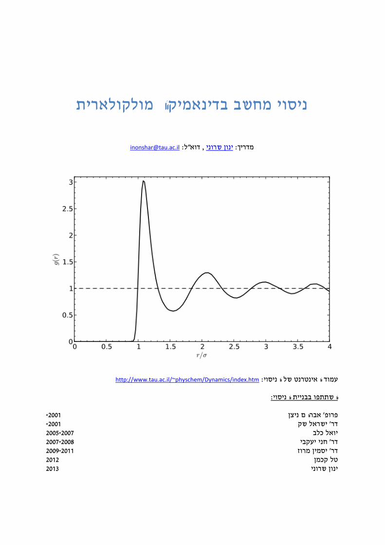
תמולקולארי הבדינאמיקי מחשב וניס
[email protected]: ל"ואד, ינון שרוני: מדריך
http://www.tau.ac.il/~physchem/Dynamics/index.htm: של הניסוי אינטרנטהעמוד
:השתתפו בבניית הניסוי
- 1002 אברהם ניצן' פרופ
- 1002 ישראל שק' דר 1002-1002 יואל כלב
1002-1002 חני יעקבי' דר 1002-1022 יסמין מרוז' דר
1021 טל קכמן 1022 ינון שרוני

Inon Sharony: מדריך ניסוי מחשב בדינאמיקה מולקולארית
1 מבוא
מבוא
הקדמה
הניסוי .חישובי ןכתיאורטיקעבודתו התנסות ראשונה ב ,ךלתלמיד המעוניין בכ ,ה להעניקמטרת ניסוי זמעבדה , שיטות נומריות: כגון םתיאורטיינוגע במספר תחומי ידע שנלמדים באופן מלא יותר בקורסים
ל לא מהווה "אף אחד מהקורסים הנ. סטטיסטית ומהלכים אקראיים תרמודינאמיקה, בכימיה חישוביתאך אין בכך לומר שמדען , התכנות הינו חלק בלתי נמנע מעבודה חישובית .שת קדם לביצוע הניסוידרי
שאלמלא כן , מסוימתבמסגרת הניסוי יבצעו התלמידים עבודת תכנות . חישובי הוא במהותו מתכנת .כמטרה אלא ככלילא תכנות ההסתכלות עלהינו הדגש , עם זאת .החוויה לא הייתה אמינה
ת מחשבסימולציו
. של מערכת נתונה ,או דגם, סימולציית מחשב היא תוכנת מחשב שמשמת להדמיית מודל מתמטי מופשטאם פתרון , כאשר מוכח שלמודל המתמטי אין פתרון אנאליטי בפתרון באמצעות מחשב לעיתים מתחיי
הם , ון נומרילעומת פתר, אם המשאבים הנדרשים למציאת פתרון אנאליטי, כלומר. ישיםשכזה פשוט אינו פתרון אנאליטי ייראה כפונקציה של משתנים ופרמטרים שבהצבתם נוכל .רבים מאשר ברצוננו להשקיע
נוכל להשתמש בשיטות קירוב מקומיות , אם אין בידנו פתרון אנליטי כללי (.נומרי)לקבל פתרון מספרי נומריות מטפלות אך ורק סימולציות . המותאם למימוש באמצעות מחשב, בכדי לבנות פתרון איטרטיבי
תכניות קיימותלמרות שכיום )בערכים המספריים של המשתנים המעורבים ולא באלגברה מופשטת (.מחשב שיודעות לעשות אפילו את זה
מידול מתמטיבצורה תלהיעשוצריך להכו: "ינשטייןיכפי שאמרו מאז אריסטו ועד א. המפתח הינו הפשטה, הדגםבבניית
.יש המכנים מימרה זו תערו של אוקאם, מסוימיםבהקשרים ." ך לא פשוט מכךא, הפשוטה ביותרולדרוש רמות משאבים הולכות וגדלות , סימולציות מחשב יכולות לכלול רמות שונות של מורכבות
ניסיונות המבוצעים במחשב לעיתים נקראים .על מבוזר-למחשובהחל מאיטרציה ידנית ועד , בהתאם ".in silico"בהתלוצצות
פתרון נומרי, הכוללים למשל מציאת אפסים וערכים עצמיים, ניתן למדל בעיות באמצעות ניסוחים מתמטיים שונים
(חשבון וריאציות ,לדוגמה)קומבינטוריקה ואופטימיזציה , הסתברות וסטטיסטיקה, גזירה ואינטגרציה .לכל ניסוח יכולות להתאים מספר שיטות נומריות למציאת הפתרון. ועוד
.לדוגמה עבור מיון וחיפוש במבני נתונים, ל"פותחו אלגוריתמים המייעלים מאד את החישובים הנ, בנוסף
יתרונות של פתרון באמצעות מחשבהוא מאפשר חשיבה אינדוקטיבית , לדוגמה. שימוש במחשב לפתרון בעיות נושא איתו כמה יתרונות
ישנם מקרים בהם , בנוסף(. מקרים פרטייםכללית מקבוצה סופית של הותיאוריהסקת אינטואיציה )כלומר )לחלוטין דטרמיניסטית הבעיהגם אם , הבעיהאקראיות המיוצרת על ידי מחשב מייעלת את פתרון
ערי ההימורים ה באמצעות משפחת האלגוריתמים על שםמפורסמת היא אינטגרצי הדוגמ(. לא אקראית .וש באקראיות נקראים אלגוריתמים סטוכסטייםאלגוריתמים שעושים שימ. ולאס ווגאס מונטה קרלו
2291, פבלו פיקאסו – ."הם יודעים לתת רק תשובות. תועלתמחשבים הם חסרי "
.במעבדה נתמקד באופן השגת תשובות אלו ובדרכים לפרשן

Inon Sharony: מדריך ניסוי מחשב בדינאמיקה מולקולארית
2 מבוא
מולקולאריתדינאמיקה
מקרוסקופיותנות היא שיטה המאפשרת שיערוך של תכו( Molecular Dynamics, MD)דינאמיקה מולקולארית צברים של ומיצוע על גביהדמיית תהליכים מיקרוסקופיים באמצעות( כגון תכונות תרמודינאמיות)
השהמכאניקתחת ההנחה , היא מבוססת על פתרון נומרי של משוואות התנועה של ניוטון. םחלקיקי .הקלאסית קבילה
?קלאסית המכאניק מדוע "?היא המושלת ביקום הקוונטיתשזו הקלאסית כאשר מסתמן הבמכאניקמדוע להשתמש " :עולה השאלה
( זמן מעבד וזיכרון)א העלייה המעריכית בצריכת משאבי מחשוב והקלאסית ה הבמכאניקהמניע לשימוש ניתן להראות שעבור מערכות , אולם. ככל שגדלה המערכת שעבורה עושים את החישוב, קוונטילפתרון
.הקלאסית מהווה קירוב טוב ההמכאניק, רבות בטווחי טמפרטורות סבירים
הפוטנציאלבחירת משטח , וכתוצאה מכך האנרגיה הפוטנציאלית של המערכת, תמולקולאריו-אטומיות והבין-האינטראקציות הבין
בחירת משטח הפוטנציאל צריכה לשקף את התכונות . תפונקציומגוון רב של ניתנות לתיאור באמצעות , לדוגמה, קיימים הן בדגמיםתכונות הנמצאות בשכיחות גבוהה . נההפיזיקאליות של המערכה הנדו
בכדי לדמות דחייה קולומבית )הדרישה ששני אטומים לא יוכלו להימצא באותה נקודה במרחב ובאותו זמן .ושהאינטראקציה תדעך במרחקים גדולים( או דחיית פאולי
כיול הפרמטריםעובדה זו הופכת את . ות שימוש במידע שהושג בניסיוןנהוג לכייל את הפרמטרים של הפוטנציאל באמצע
.אמפירי מטבעו-החישוב לסמי
Inon Sharony: מדריך ניסוי מחשב בדינאמיקה מולקולארית
1 מבוא
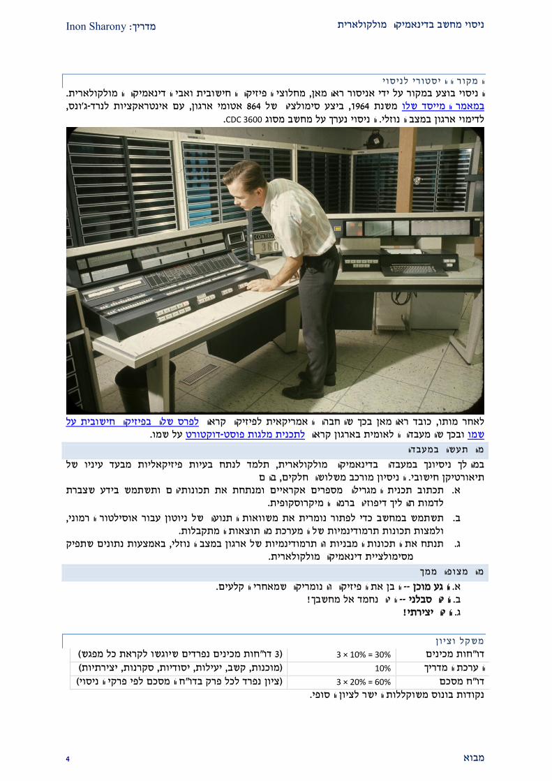
ניסויההיסטורי למקור ה. המולקולאריתמחלוצי הפיזיקה החישובית ואבי הדינאמיקה , הניסוי בוצע במקור על ידי אניסור ראהמאן
, ונס'ג-עם אינטראקציות לנרד, אטומי ארגון 291של סימולציהביצע , 2291משנת אמר המייסד שלובמ .CDC 3600הניסוי נערך על מחשב מסוג . לדימוי ארגון במצב הנוזלי
לפרס שלה בפיזיקה חישובית על כובד ראהמאן בכך שהחברה האמריקאית לפיזיקה קראה , לאחר מותו
.על שמו דוקטורט-לתכנית מלגות פוסטובכך שהמעבדה הלאומית בארגון קראה שמו
עשה במעבדהתמה
זיקאליות מבעד עיניו של תלמד לנתח בעיות פי, תמולקולאריבמהלך ניסיונך במעבדה בדינאמיקה בהם, הניסיון מורכב משלושה חלקים .חישובי ןתיאורטיק
ותשתמש בידע שצברת ומנתחת את תכונותיהם מספרים אקראייםב תכנית המגרילה וכתת .א .לדמות תהליך דיפוזיה ברמה המיקרוסקופית
, הרמוניעבור אוסילטור ניוטוןהתנועה של כדי לפתור נומרית את משוואות תשתמש במחשב .ב .המתקבלות התוצאותשל המערכת מ דינמיותתרמותכונות מצות ול
באמצעות נתונים שתפיק , במצב הנוזלי ארגוןתנתח את התכונות המבניות והתרמודינמיות של .ג .תמולקולארי הדינאמיקמסימולציית
מה מצופה ממך
.הבן את הפיזיקה והנומריקה שמאחרי הקלעים -- הגע מוכן. א !היה נחמד אל מחשבך -- בלניהיה ס. ב !היה יצירתי. ג
וציון משקל
(חות מכינים נפרדים שיוגשו לקראת כל מפגש"דו 2) 30% = 10% × 3 חות מכינים"דו (יצירתיות, סקרנות, יסודיות, יעילות, קשב, מוכנות) 10% הערכת המדריך
(רקי הניסויח המסכם לפי פ"ציון נפרד לכל פרק בדו) 60% = 20% × 3 ח מסכם"דו.נקודות בונוס משוקללות הישר לציון הסופי

Inon Sharony: מדריך ניסוי מחשב בדינאמיקה מולקולארית
2 מבוא
הענייניםתוכן
1 ................................................................................................................................................................ מבוא 1 ......................................................................................................................................................... הקדמה
1 ........................................................................................................................................ מחשב סימולציות
2 ............................................................................................................................... מולקולארית דינאמיקה
1 ..................................................................................................................................... במעבדה תעשה מה
1 ........................................................................................................................................... ממך מצופה מה
9 ............................................................................................................................................... לניסוי הכנות
2 ................................................................................................................................ המסכם ח"לדו דרישות
21 ............................................................................................................................ המעבדה יפורלש הערות
21 ................................................................................. האוניברסיטאיים המחשוב במשאבי מרוחק שימוש
22 ............................................... (הפשוט האקראי המהלך: בוחן מקרה) סטוכסטיים תהליכים סימולציית .א
22 .................................................................................................................................. הניסוי של זה בשלב
22 .............................................................................................................................................. קריאה חובת
22 ................................................................................................................................................... מכין ח"דו
21 ............................................................................................................................................. הניסוי ביצוע
22 .................................................(הרמוני בפוטנציאל תנועה: בוחן מקרה) ניוטונית מכאניקה סימולציית. ב
22 .................................................................................................................................. הניסוי של זה בשלב
22 .............................................................................................................................................. קריאה חובת
19 ................................................................................................................................................... מכין ח"דו
12 ............................................................................................................................................. הניסוי ביצוע
22 ....................................... (נוזלי ארגון של משקל שיווי: בוחן מקרה) מולקולארית דינאמיקה סימולציית. ג
22 .................................................................................................................................. הניסוי של זה בשלב
22 .............................................................................................................................................. קריאה חובת
99 ................................................................................................................................................... מכין ח"דו
92 ............................................................................................................................................. הניסוי ביצוע

Inon Sharony: מדריך ניסוי מחשב בדינאמיקה מולקולארית
9 מבוא
הכנות לניסוי
ים שיש לשאולספר
(חובה)מקורות עיקריים
:ירקע תיאורט .א Abraham Nitzan, Chemical Dynamics in Condensed Phases, Oxford University
Press (2006).
:המולקולארית הדינאמיקהשיטת .ב Daan Frenkel & Berend Smit, Understanding Molecular Simulations, Second Edition, Academic
Press (2002).
מקורות נוספים
:פתרון נומרי של משוואות ניוטון .ג
Gould & Tobochnik, An Introduction to Computer Simulation Methods, third edition, Pearson
(2007).
:של נוזליםת וסימולצי .ד A.Rahman, "Correlations in the Motion of Atoms in Liquid Argon," Phys. Rev. A 136 P. A405, 1964.
L. Verlet, "Computer Experiments on Classical Fluids. I. Thermodynamical Properties of Lennard-
Jones Molecules," Phys. Rev. 159, 98 (1967).
D. W. Heermann, Computer Simulation Methods in Theoretical Physics, second edition, Springer
(1990).
M.P. Allen & D.J. Tildesley, Computer Simulation of Liquids, Oxford University Press (1991). A 2003
version also exists.
:וקורלציה בזמן מספרים אקראיים .ה Frederick Reif, Fundamentals of Statistical and Thermal Physics, McGraw-Hill (1965). A 2008
version also exists.
:פונקציות קורלציה מרחביות של נוזלים .ו David Chandler, Introduction to Modern Statistical Mechanics, Oxford University Press (1987).
קריאה להרחבה
:שיטות נומריות .ז Steven E. Koonin & Dawn C. Meredith, Computational Physics: FORTRAN Version, Addison-Wesley
(1990).
Richard J. Sadus, Molecular Simulation of Fluids: Theory, Algorithms and Object-Orientation, Elsevier (2002).
Numerical Recipes: The Art of Scientific Computing, Third Edition (C++), Cambridge University
Press (2007). Limited free access on www.nr.com (full access for second edition 1992 in C or
FORTRAN).
:תכונות של נוזלים .ח
Jean-Pierre Hansen & I.R. McDonald, Theory of Simple Liquids, 3rd
edition, Academic Press (2006).

Inon Sharony: מדריך ניסוי מחשב בדינאמיקה מולקולארית
2 מבוא
להכנה הנחיות
ח מכין"הנחיות להכנת דו
ח "הדוהגישו את , רלוונטי בתדריךההחומר המופיע תחת הפרק כל קראו את ,לקראת כל פגישה .2 .גם במעבדהנוספות ות על שאלות היו מוכנים לענוהמכין
.את שמותיכם בקבצים שאתם שולחים לי כדי שלא אתבלבל ביניכם כתבואנא .1
tמבחן , שגיאה יחסית)בתוספת עמודת השוואה , יש לערוך בטבלה תשובות לשאלות השוואה .2 (.Welchשל
ן לי דרך ללא נימוק התוצאות אי. ניקוד מלא יינתן רק אם תקושר התוצאה לעקרונות שנלמדו .1 .לדעת שהבנתם למה התקבלה דווקא תשובה זו
יש , בכדי שאספיק לבדוק את שאלות ההכנה שלכם לפני שתתחילו בביצוע כל שלב בניסוי .2ח המכין שהגשתם "הקפידו לעבור על הדו. ח המכין עד יום לפני ביצוע המעבדה"להגיש את הדו
וזאת , תחילו את ביצוע המעבדהבטרם ת, ולוודא שאתם מבינים את כל הטעויות שנמצאו בו .בכדי למנוע גרירת שגיאות
הנחיות להכנה לתכנות
פנו אל המדריך מיד , LINUXאו קומפילציה שלו בסביבת Cבמידה ואינכם שולטים בכתיבת קוד .9 Cשפת התכנות יכולה להיות שונה מ , בחלקי הניסוי בו נדרשת כתיבת קוד .עם קבלת תדריך זה
, (Micro$oft Visual Studio או ++Dev-C לדוגמה) לבחירתכם, LINUXמ וסביבת ההפעלה שונה .Cאך חלק מהניסוי כבר כתוב בשפת
בחלק האחרון של . תוכלו לכתוב בכל שפת תכנות שתבחרואך , C מערך הניסוי נכתב עבור שפת .2את ולשם כך עליכם להכיר את השפה מספיק בכדי להבין ( Cב)הניסוי תעשו שימוש בקוד כתוב
. פעולת הקוד וכיצד להשתמש בתוצריו באמצעות שפת התכנות שתבחרו לעבוד בה .MATLAB סטודנטים ביצעו בעבר את המעבדה ב, לדוגמה
ורנשטיין אניתן לבצע את המעבדה על מחשב ייעודי במעבדת המחשבים של בית הספר בבניין .2ם ולבצע את הניסוי באופן ניתן להשתמש במשאבי המחשוב האוניברסיטאיי, לחלופין. 202חדר
/home/stud1/בשם ת הבית שלכםתיקייו, stud1לשירותכם שם המשתמש .(ראה הערות) מרוחק .alpc-mdהינה stud1משתמש סיסמת ה .על הכונן הקשיח
הנחיות להגשות
וכתב, ביצוע כל פרק בניסוי( או תוך כדי)מיד לאחר .סיקרו את כלל התדריך ושימו לב לדגשים .2ח "חשובות לא ישכחו עד זמן כתיבת הדו שתובנותעל מנת ,קרי הממצאים והמסקנותאת ע
.המסכם
ח המסכם של "תאריך היעד להגשת הדו, משמעיות של פרופסור אבן-בהתאם להנחיותיו החד .20ח עד תאריך זה "מי שלא יגיש את הדו. הניסוי הוא עד היום שלפני תחילת הניסוי הבא שלכם
!יסוי הבאלא יוכל להתחיל את הנ

Inon Sharony: מדריך ניסוי מחשב בדינאמיקה מולקולארית
2 מבוא
ח המסכם"דרישות לדו
ללא תלות במועד , ח המסכם יוגש לפחות יומיים לפני הפגישה הראשונה בניסוי הבא"הדו .2 .לא תוכלו להמשיך לניסוי הבא, ולא. ביצוע הפרק האחרון בניסוי הנוכחי
tמבחן , שגיאה יחסית)גדלים יחסיים , למען הבהירות .ספרות ערך ויחידותיש לשמור על מספר .1
.(arbitrary units)ולציין שהיחידות שרירותיות להציג באחוזיםיש ( 'וכו
.השוואות בין מספר גדלים יש להציג בטבלה .2 דיווח הערכת שגיאה .1
הינה הגדולה הערכת השגיאה .יש לצרף לכל גודל מספרי מדווח גם הערכת שגיאה .אסטיית התקן )טית השגיאה הסטטיסו( ספרות ערך, דיוק מדידה) המערכתיתמבין השגיאה
(.של המדגם שהממוצע שלו הוא הגודל המדווח
תלויים ולחשב -יש לבצע הערכת שגיאה עבור הגדלים הבלתי, עבור גדלים תלויים .ב (.פרופגציה של שגיאות)את השגיאה הנגזרת
, שגיאה יחסית) יש להקפיד על דיווח יחידות ומרווחי שגיאות בדיווח תוצאות: דיוק .גיש להסביר כיצד ניתן לשפר את . להבחין בין שגיאה מוחלטת ליחסיתהקפידו .(לדוגמה
.השגיאה בתוצאות החישוב( או אנליטיקה ןניסיו)יש להשוות תוצאות מחושבות לתוצאות מהספרות : נכונות .ד
ולנסות , יש להתייחס אל אי התאמה בין השתיים כאשר ישנו .בכל הזדמנות אפשריתשיקולים , כיצד ניתן לשפר את החישוב, לדוגמה)להסביר כיצד ניתן ליישב את הפער יש , (ראה סעיף קודם)במידה ויש הערכת שגיאה (. פיזיקאליים שבאים לידי ביטוי או שלא
:Welchשל tלהציג גם את תוצאת מבחן
t = (xcalculated – xexpected) / √(2
calculated + 2
expected/n expected)
2
calculated = √(2
systematic + 2statistic/nsamples)
להצדיק את השימוש בפונקציה שנבחרהיש , בהתאמת נתונים לפונקציה אנליטית .2
?מה המודל שעומס בבסיס ההנחה שהפונקציה אכן מתארת את הנתונים .א פונקציתשל כל אחד מהפרמטרים המופיעים במשוואת תהפיזיקאליהמשמעות מה .ב
לי ממדים כארגומנטים לפונקציות שימו לב לא להשאיר גדלים בע)? ההתאמה (אלא לחלק בפרמטר בעל אותן יחידות' לוגריתמיות וכו, מעריכיות, טריגונומטריות
2) טיב ההתאמהמה האומדים ל .ג/2*ndfχp~, R
?('וכו2
.על מנת לקבל ניקוד מלא הציגו את הידע שצברתם במהלך המעבדה, בניתוח התוצאות .9 :ח"מבנה הדו .2
תאריכי ביצוע , שמות הכותבים ודואר אלקטרוני שלהם, עמוד שער הכולל כותרת .א (:משפט לכל אחד)המפרטת את הבאים תקציר ופיסקת, והגשה
.מטרות הניסוי (2) .עיקרי הממצאיםפרטו את (1) .עיקרי המסקנותציינו את (2)
.ח"וכל פרק בניסוי יתואר בפרק נפרד בדו, את גוף העבודה יקדים תוכן עניינים .ב :ח"הקדמה לכלל הדו .ג
אלו תופעות או בעיות פיזיקאליות מטופלות :והיקפו של הניסויההקשר (2)שלכות המהן ה? מה החשיבות של ההתעסקות בנושא? או משפיעות בעקיפין
?אפשריות של התקדמות בתחוםה .עם סימוכין ,תוצאות רלוונטיות מניסויים שבוצעו בעבר (1) .שבאים לידי ביטוי יעקרונות מהרקע התיאורט (2) .חות המכינים"פי כל אחד מהדו התוצאות הצפויות על (1)

Inon Sharony: מדריך ניסוי מחשב בדינאמיקה מולקולארית
2 מבוא
ביצועפרקי ה .ד
נא הפעילו שיקול ) בראשית כל פרק יופיע תיאור של מטרות אותו פרק (2) (.לעתיק מהתדריך דעת והשתדלו לא
מה : והשיקולים בבנייתו ובחירת הגישה לפתרונו, תיאור המודל שנחקר (1)משוואות מהן ה .אור נכון של הבעיהיקיבל ייצוג ומה הוזנח כפחות קריטי לת
('וכו? מהן משוואות התנועה? האנרגיה פונקציתמה ההמילטוניאן או ) ?שנפתרובהן נעשה שימוש בחלק זה של הניסוי שיטות ניתוח התוצאותפירוט (2)
.והסיבות לבחירתן( כולל הצגת נוסחאות רלוונטיות) לב שימו. ח"בדו נפרד כסעיף תופיע בתדריך שאלה כל אל תההתייחסו (1)
.סעיף פספסתם שלא וודאו .הסעיפים לכלברוב מעבדי התמלילים יש אפשרות ) ואיור טבלה, משוואה כל מספור (2)
. (עם הוספתן, איוריםו טבלאות, אוטומטי של נוסחאות למספור הממצאים עיקרי את בקצרה המתאר ואיור טבלה לכל מתחת כיתוב הוספת
המשוואה היהת 2.א משוואה, לדוגמה) פרק לפי למספר לבחור תוכלו. המוצגים (.'א בפרק השלישית
בסוף כל פרק יופיע נספח בו יפורטו כלל הפרמטרים וקוד התוכנה (9)תיאור ) חובה לכתוב הערות בגוף הקוד .הנדרשים לשחזור מלא של הניסוי
כמעט בכל שורה , אם תעשו זאת כראוי(. פעולתה של כל פונקציה וחלק בתכניתחישוב אנרגיה קינטית ", " מקובץקריאת קלט ", לדוגמה)שנייה תהיה הערה
(.'וכו, "ממהירויות
השוואה בין התוצאות הצפויות לאלו , ח"דוהתוצאות המרכזיות שהוצגו בסיכום של .הניסוי לקראת לניתן ורצוי להמליץ על שיפורים , בנוסף. ומסקנות, שהתקבלו בפועל
.המשתתפים הבאים ביבליוגרפיה .ו
(יינתן בונוס) פורמט ההגשההמלצות .2 .בסביבה התחשבות מתוך( מודפס לא) אלקטרוני בפורמט ח"הדו את לקבל שמחא .א
, PDFפורמט ל Wordלייצא קובץ , לדוגמה. Micro$oftלא להגיש בפורמט .ב .נוח להצגה והוספת הערות שהוא
ח "הפרקים השונים בדו-שימוש בכותרות מובנות לפרקים ותתי, ברוב מעבדי התמלילים .ג .PDFץ וכן עניינים ואינדקס לקובטי של תיאפשר ייצור אוטומ
.אך הוא יתקבל גם בעברית, באנגליתח "מומלץ להגיש את הדו .ד
.ח בשתי עמודות בכל עמוד"מומלץ לערוך את הדו .ה

Inon Sharony: מדריך ניסוי מחשב בדינאמיקה מולקולארית
20 מבוא
דיווח תוצאות והשוואה לדוגמה
Statistical tests
Precision Accuracy Value Parameters Measurement /Calculation
Welch's t-test
Overall precision
Expected deviation
Statistic spread
Measurement resolution
Relative error
Absolute error
Expectation value
Sample mean
Sample size
Moment Distribution
No. nx
t N nxN .
n
ana
xN .
n
num
xN
.
n
res x nxN nx
N nE x nx
N N n f x
(9) (8) (7) (6) (5) (4) (3) (2) (1)
144% 0.026 0.026 0.026 1510 -2.4% -0.012 0.500 0.488 10 1 1 1
68% 0.30 0.32 0.30 1510 1.0% 0.03 3.19 3.23 100 2 exp x 18
(1) 1
1n
Nn n
ix Ni
N x xN
(4) n
n
x
nx
NN
E x
(7)
.
2
2
var sd
1
n
n n
ana
x
n n
x xN
N N
f x x dx f x x dxN
(2) n nE x f x x dx
(5)
1 1
.
1
15
. double-prec.
1
10
n n n
res
n
n
res
x x x x
x
x
(8)
2
2.
n n
n
res
x x
xN N
N
(3) n n
n
x xN N E x (6)
2
. 2
2
2
1 1
1 1
n
num n n
x N N
N Nn n
i i
i i
N x x
x xN N
(9)
2 2
. .
n
n
n n
x
xnum ana
x x
Nt N
N N

Inon Sharony: מדריך ניסוי מחשב בדינאמיקה מולקולארית
22 מבוא
טיב התאמהיש להצדיק את בחירת פונקצית . התאמת הפלט המספרי לפונקציה אנליטית אינו עניין של מה בכך
לכל סט של :טיב ההתאמה אינו מקרי, ולהראות שבסבירות גבוהה, ההתאמה משיקולים פיזיקאליים
N נקודות נוכל להתאים פולינום מדרגהN-1 ערךבהכרח כל התאמה כזו אין אולם ל, באופן מדויק.
R2
נבטא , Xiביחס לסט המדידות , iבנקודות המדידה fשל פונקצית ההתאמה את טיב ההתאמה
סכום ריבועי השאריות ו( Explained Sum of Squares, ESS)סכום הריבועים המוסבר באמצעות
(Residual Sum of Squares, RSS):
1
2 22
1 1
2 2
1 1
1
1 1
1 1
N
X i
i
N N
X i X i i
i i
N N
i X i i X
i i
XN
SS X RSS X fN N
ESS f WSSR w XN N
, wiמשקל פונקציתהוספנו אפשרות להכליל את הביטוי באמצעות , שורה האחרונהכאשר ב, (י מתן משקל גדול יותר לנקודות המתועדפות"ע)על פני אחרות מסוימותמדידות תעדוףהמאפשרת
.Weighted Sum of Squares of Residuals -ה לקבלתהתרומה שאריות הוא ה בועיירואילו סכום , בר ניתן לפירוש כשונות המוסברתסוהריבועים המכום ס
.לשונות שאינה מוסברת על ידי ההתאמה
(coefficient of determination)טיב ההתאמה לפעמים ניתן באמצעות מקדם הקביעה
2 1ESS RSS
RSS SS
ההתאמה שפונקציתבין הערכים ( Pearsonשל )מקדם הקורלציה של כריבועביטוי זה ניתן לפירוש Rערך , לפיכך .מנבאת לבין הערכים שניתנו בסט המדידות
פונקציתאפסי משמעו שאין קורלציה בין 2 .(חיובית או שלילית) ד משמעו שישנה קורלציה כזווערך הקרוב לאח, ההתאמה לבין המדידות
2
באמצעות , צפויהניתן גם לקבל מדד לטיב ההתאמה בין התפלגות גדלים שנמדדה לבין התפלגות
2) כי בריבוע מבחן
). לשם כך נחשב את
2
1
Ni i
i i
X f
f
הקשרים מספר המדידות פחות מספר כלומר , =N-p, נספור את מספר דרגות החופש, לאחר מכןנשווה את הערכים שחושבו מול הערכים הצפויים , לבסוף .המבטאים תלות בין הפרמטרים של הבעיה
2ות מהתפלג
( 2 ערכים תיאורטיים עבור התפלגות טבלתבאמצעות
) מידת אומדן לונקבל
הגודל המביע .של ההתאמה בין הפונקציה שנבחרה לבין המדידות שהיא אמורה לתאר המובהקות
.2%ובדרך כלל נדרוש ערך הקטן מ , p-value מובהקות נקרא

Inon Sharony: מדריך ניסוי מחשב בדינאמיקה מולקולארית
21 מבוא
המעבדה ורלשיפ הערות
:דרישות(. חלונות כגון) LINUX שאיננה עבודה בסביבת גם זה ניסוי לבצע אפשרת מתן .2
הפלט טווח, לדוגמה) בו לשימוש מותאם והקוד, מתאים אקראיים מספרים מחולל נמצא .א (.שונה להיות עלול המחולל של
.כראוי עובדת נוזלי ארגון של לסימולציה שימוש נעשה שבה המוכנה התוכנית .ב
של -ה ומשפט ריילי שיטת :מימדים אנאליזת לנושא קריאה מקורות למצוא .1 .באקינגהם
םהאוניברסיטאיי המחשוב במשאבי מרוחק שימוש
באמצעות שימוש בקליינט gpניתן לפתוח מסך שמציג שולחן עבודה מרוחק על גבי השרת .2
Citrix.
באמצעות שם המשתמש והסיסמא סלהיכניש , לאחר התקנת הקליינט .א (.@לפני ה , ל שלך"מה שמופיע בכתובת הדוא, כלומר) האוניברסיטאיים
.Exceedוביישום Terminal emulationלבחור בתיקיית יש .ב
.Lingoהשרת דרךיש להתחבר .ג
לעמוד בדפדפן גלישה י"ע Java applet הפעלת, לחלופין .1
http://gate.tau.ac.il
.LINUXעובד בסביבת חלון הטרמינל שייפתח .אישור בטחוני להפעלת היישום ומתן
על ידי הקשת (general processing)יש להתחבר לשרת לשימוש כללי .2
ssh gp
.ולהזין שוב את הסיסמא האוניברסיטאית
:נבצע קומפילציה ונריץ, Cנכתוב תוכנית פשוטה ב , לצורך ההדגמה .1
VIMלכתיבה באמצעות התמלילן HelloWorld.cנתחיל בפתיחת קובץ בשם .א על ידי הקלדת
vim HelloWorld.c
לא משנה איפה נתחיל את , היות והקובץ ריק)להתחיל מצב כתיבה אחרי הסמן .ב
.a לוחצים (הכתיבה :כעת ניתן לכתוב את הקוד כדלקמן
#include <stdio.h>
#include <math.h>
int main(){
printf("Hello World!\n");
printf("%e\n",exp(1));
return 0;
}
wq: שמירת הקובץ ויציאה מהתמלילן נקליד, לסיום מצב כתיבה .ג
נבצע קומפילציה של התכנית תוך שימוש בכל . כעת חזרנו את חלון הטרמינל .ד נעשה זאת על ידי הקלדת . האזהרות ההתראות שהוא יודע להציע
gcc –g3 –O0 –Wall –Wextra –lm HelloWorld.c –o HelloWorld.out
:כךנריץ אותה , בהנחה שהתכנית עברה קומפילציה ללא הודעות שגיאה .ה
./HelloWorld.out
ובעקבותיה כתובת wgetהפקודה ניתן להוריד קבצים מהאינטרנט באמצעות .ו
.)כולל כל הקידומות)הקובץ
.exitויציאה נקליד gpלסיום השימוש בשרת .ז
(פעמיים)החיבור אל מחשבי האוניברסיטה נקליד וסגירת sshלסיום השימוש ב .ח
exit

Inon Sharony: מדריך ניסוי מחשב בדינאמיקה מולקולארית
22 (המהלך האקראי הפשוט: מקרה בוחן)תהליכים סטוכסטיים יתסימולצי .א
(המהלך האקראי הפשוט: מקרה בוחן)תהליכים סטוכסטיים יתסימולצי .א
בשלב זה של הניסוי
ת ומערכו ותממצומצ הצגותועל ,כמקור לאקראיות תלמדו על החלוקה בין מערכת לסביבה .2 .ותפתוח
.להשתמש בהם בתיאורים פיזיקאלייםכיצד ניתן הם מספרים אקראיים וה תלמדו מ .1
.תלמדו תכונות של מספרים אקראיים וכיצד תכונות אלו מאפיינות את התהליך שיצר אותם .2
.מידע מהםתתרגלו הגרלת מספרים אקראיים והפקת .1 .תלמדו כיצד מבצעים סימולציות סטוכסטיות .2
קריאהחובת
וסימולציה שלהם סטוכסטייםתהליכים
מבוא )רק הראשון והשלישי הפ-תתיש להתמקד בעיקר ב. עמודים הבאיםחומר הרקע בקראו את .2 (.בהתאמה, לתהליכים סטוכסטיים וסימולציות נומריות של תהליכים סטוכסטיים
.ניצן מאת "Chemical Dynamics in Condensed Phases" בספר 7.1-7.2 -ו 1.5 משנה יפרק קראו .1
:רשות תקריא (השיכור מהלך) יאקרא ומהלך ההסתברות לתורת מבוא
,או לחליפין .ניצן מאת "Chemical Dynamics in Condensed Phases" בספר 2.2 משנה פרק קראו .22. Frederick Reif, "Elementary probabilistic & statistical concepts and examples, and the simple random
walk in 1-D" (pp. 4-24) in Fundamentals of Statistical and Thermal Physics, McGraw-Hill (1965). A
2008 version also exists.
Inon Sharony: מדריך ניסוי מחשב בדינאמיקה מולקולארית
21 (המהלך האקראי הפשוט: מקרה בוחן)תהליכים סטוכסטיים יתסימולצי .א
INTRODUCTION TO STOCHASTIC PROCESSES
ABRAHAM NITZAN, CHEMICAL DYNAMICS IN CONDENSED PHASES,
OXFORD UNIVERSITY PRESS (2006).
The motivation for using probabilistic concepts in the description of chemical processes in
condensed phases is the same as for using such concepts in statistical mechanics: There we
are facing the need to treat macroscopic systems on a microscopic level, focusing only on a
few observable quantities such as energy, pressure, temperature, etc. In the reduced space of
these observables, the microscopic influence of the other ~ 1023
degrees of freedom gives
these observables a random character. Most often we measure just the averages of these
quantities, but their fluctuations are observable too.
When discussing processes involving a single molecule in condensed phases the
observables are molecular, essentially microscopic properties. Still, as before we focus on a
few observables associated with the chemical or physical process of interest. Processes
described in the reduced space of these variables are stochastic, and the variables themselves
are random.
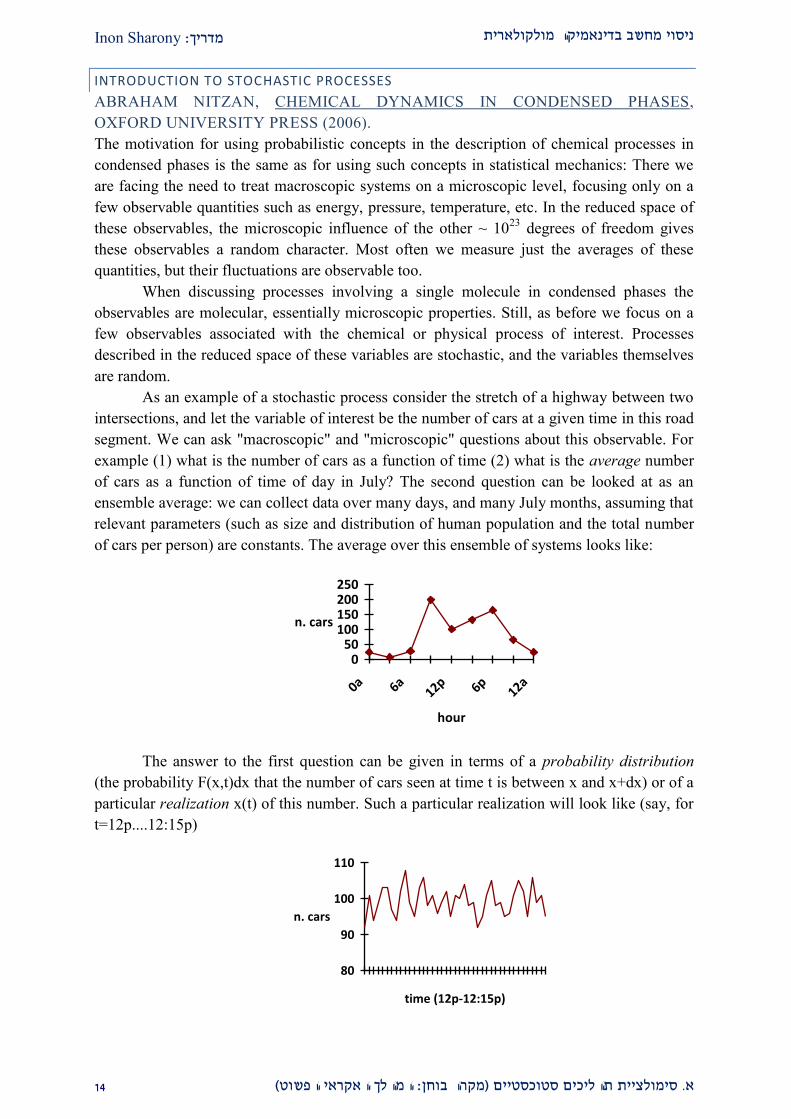
As an example of a stochastic process consider the stretch of a highway between two
intersections, and let the variable of interest be the number of cars at a given time in this road
segment. We can ask "macroscopic" and "microscopic" questions about this observable. For
example (1) what is the number of cars as a function of time (2) what is the average number
of cars as a function of time of day in July? The second question can be looked at as an
ensemble average: we can collect data over many days, and many July months, assuming that
relevant parameters (such as size and distribution of human population and the total number
of cars per person) are constants. The average over this ensemble of systems looks like:
050
100150200250
0a 6a12p 6p
12a
hour
n. cars
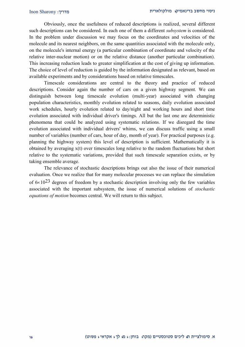
The answer to the first question can be given in terms of a probability distribution
(the probability F(x,t)dx that the number of cars seen at time t is between x and x+dx) or of a
particular realization x(t) of this number. Such a particular realization will look like (say, for
t=12p....12:15p)
80
90
100
110
time (12p-12:15p)
n. cars

Inon Sharony: מדריך ניסוי מחשב בדינאמיקה מולקולארית
22 (המהלך האקראי הפשוט: מקרה בוחן)תהליכים סטוכסטיים יתסימולצי .א
Obviously if we repeat the "experiment" during the same time window the next day,
this graph will look different. If we repeat this experiment enough times we can evaluate the
probability distribution F(x,t). For this purpose we can draw an histogram showing, for N
"experiments", the number ni of experiments which gave number of cars between xi and xi+
x ( n Ni
i
), at time t. F(x,t) is then the limit, as N, of ni/N. The following points
should be noticed:
(1) The function F(x) defined above was constructed as a continuous probability
density even though for the example considered x take only integer values. This description
is useful when x >> 1 (a prerequisite is that the range of interest is xi>>>1). This is an
example of coarse graining: looking at F(x) only at resolution poorer than x
(2) Another example of coarse graining: coarse graining in time. If instead of
displaying x(t) as a function of t every minute(say) we will display 10-minutes averages of
x(t) (namely redefine 5
5
( ) (1/10) ( )i
i
i
x t x t
) we will eliminate fluctuations on the fast
timescale: The new stochastic variable ( )x t will fluctuate only on timescale > 10. Provided
that the timescale associated with the systematic variation of the ensemble average <x(t)> is
much slower than that associated with the random fluctuations of x(t), we intuitively expect
that the coarse grained variable ( )x t resembles the ensemble average <x(t)>. The conditions
for this expectation to materialize are quite complicated. In equilibrium statistical mechanics
this issue is discussed within the Ergodic Theorem.
On the microscopic level we shall often refer to the internal (vibrational) energy of a
solute molecule as a particular example. Consider a diatomic molecule, e.g. CO, in a simple
solvent (e.g. Ar). We can monitor its vibrational energy contents by spectroscopic methods,
and we can follow processes such as thermal (or optical) excitation and relaxation, energy
transfer and migration. The quantity of interest is the average vibrational energy per
molecule, the average is over all molecules of this type in the system. At low concentration
these molecules do not affect each other and all the information can be obtained by observing
(or theorizing on) a single molecule. Average over many such molecules is an ensemble
average. Following vibrational excitation, it is often observed that the subsequent relaxation
is exponential, <E(t)>=E(0)exp(-t). The actual instantaneous energy is however much more
complicated. To predict its course of evolution exactly we need to know the initial positions
and velocities of all the particles in the system, then to solve the Newton or the Schrödinger
equation with these initial conditions. On this level of description which includes the entire
phase space of the system, the evolution is completely deterministic. However focusing only
on E(t), its detailed time evolution looks random, In particular, it will look different in
repeated experiments because in setting up such experiments only the initial value of E is
specified, while the other degrees of freedom are subjected only to a few conditions (such as
a given overall averaged kinetic energy, i.e. temperature). In this reduced description E(t)
may be viewed as a stochastic variable. The role of the theory is to set up its statistical
properties and to investigate its consequences.
Inon Sharony: מדריך ניסוי מחשב בדינאמיקה מולקולארית
29 (המהלך האקראי הפשוט: מקרה בוחן)תהליכים סטוכסטיים יתסימולצי .א
Obviously, once the usefulness of reduced descriptions is realized, several different
such descriptions can be considered. In each one of them a different subsystem is considered.
In the problem under discussion we may focus on the coordinates and velocities of the
molecule and its nearest neighbors, on the same quantities associated with the molecule only,
on the molecule's internal energy (a particular combination of coordinate and velocity of the
relative inter-nuclear motion) or on the relative distance (another particular combination).
This increasing reduction leads to greater simplification at the cost of giving up information.
The choice of level of reduction is guided by the information designated as relevant, based on
available experiments and by considerations based on relative timescales.
Timescale considerations are central to the theory and practice of reduced
descriptions. Consider again the number of cars on a given highway segment. We can
distinguish between long timescale evolution (multi-year) associated with changing
population characteristics, monthly evolution related to seasons, daily evolution associated
work schedules, hourly evolution related to day/night and working hours and short time
evolution associated with individual driver's timings. All but the last one are deterministic
phenomena that could be analyzed using systematic relations. If we disregard the time
evolution associated with individual drivers' whims, we can discuss traffic using a small
number of variables (number of cars, hour of day, month of year). For practical purposes (e.g.
planning the highway system) this level of description is sufficient. Mathematically it is
obtained by averaging x(t) over timescales long relative to the random fluctuations but short
relative to the systematic variations, provided that such timescale separation exists, or by
taking ensemble average.
The relevance of stochastic descriptions brings out also the issue of their numerical
evaluation. Once we realize that for many molecular processes we can replace the simulation
of 61023 degrees of freedom by a stochastic description involving only the few variables
associated with the important subsystem, the issue of numerical solutions of stochastic
equations of motion becomes central. We will return to this subject.
Inon Sharony: מדריך ניסוי מחשב בדינאמיקה מולקולארית
22 (המהלך האקראי הפשוט: מקרה בוחן)תהליכים סטוכסטיים יתסימולצי .א
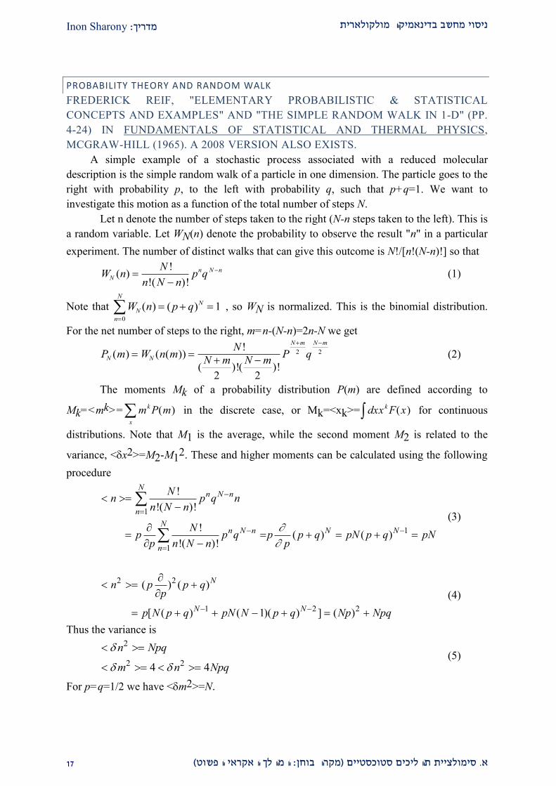
PROBABILITY THEORY AND RANDOM WALK
FREDERICK REIF, "ELEMENTARY PROBABILISTIC & STATISTICAL
CONCEPTS AND EXAMPLES" AND "THE SIMPLE RANDOM WALK IN 1-D" (PP.
4-24) IN FUNDAMENTALS OF STATISTICAL AND THERMAL PHYSICS,
MCGRAW-HILL (1965). A 2008 VERSION ALSO EXISTS.
A simple example of a stochastic process associated with a reduced molecular
description is the simple random walk of a particle in one dimension. The particle goes to the
right with probability p, to the left with probability q, such that p+q=1. We want to
investigate this motion as a function of the total number of steps N.
Let n denote the number of steps taken to the right (N-n steps taken to the left). This is
a random variable. Let WN(n) denote the probability to observe the result "n" in a particular
experiment. The number of distinct walks that can give this outcome is N!/[n!(N-n)!] so that
W nN
n N np qN
n N n( )!
!( )!
(1)
Note that W n p qN
N
n
N
( ) ( )
10
, so WN is normalized. This is the binomial distribution.
For the net number of steps to the right, m=n-(N-n)=2n-N we get
P m W n mN
N m N mP qN N
N m N m
( ) ( ( ))!
( )!( )!
2 2
2 2 (2)
The moments Mk of a probability distribution P(m) are defined according to
Mk=<mk>= m P mk
x
( ) in the discrete case, or Mk=<xk>= dxx F xk ( )z for continuous
distributions. Note that M1 is the average, while the second moment M2 is related to the
variance, <x2>=M2-M12. These and higher moments can be calculated using the following
procedure
1
1
1
!
!( )!
!( ) ( )
!( )!
Nn N n
n
Nn N n N N
n
Nn p q n
n N n
Np p q p p q pN p q pN
p n N n p
(3)
2 2
1 2 2
( ) ( )
[ ( ) ( 1)( ) ] ( )
N
N N
n p p qp
p N p q pN N p q Np Npq
(4)
Thus the variance is
2
2 24 4
n Npq
m n Npq
(5)
For p=q=1/2 we have <m2>=N.

Inon Sharony: מדריך ניסוי מחשב בדינאמיקה מולקולארית
22 (המהלך האקראי הפשוט: מקרה בוחן)תהליכים סטוכסטיים יתסימולצי .א
What is the relation of this result to the actual process of diffusion? In order to make
the connection let l be the step length, and - the step time. Thus, N steps correspond to the
total elapsed time t=N, and the final distance of the particle from the origin is the random
variable x=ml. We have found that for a symmetric random walk <x2>=l2<m2>
=l2N=(l2/)t. The factor l2/ can be estimated from molecular arguments: l is expected to be
of the order of the mean free path, 1)( , where is the molecular cross-section and is the
density. is of the order of the time between collisions, l/v, where v is the thermal velocity,
v= /Bk T m . This leads to l2/= /Bk T m /().
Compares this to what is obtained from the diffusion equation
22
2
( , ) ( , )( , )
F x t F x tD F x t D
t x
, (6)
where F(x,t) is the probability density to find the particle at x at time t. This leads to
2
20
x F F FD x D x
t x xx
(7)
provided that F0 faster than x. Similarly
2 2
2
22 2 2
x F FD x D x D F D
t xx
(8)
Since <x2>t=0=0 we found that <x2>t=2Dt, and, comparing to the result of the random walk
calculation, we see that if we require both formulations to yield the same result, then
Dl
2
2 (9)
Note that the random walk problem was handled in discrete space while the diffusion was
considered as a continuous process. To see the connection between the two descriptions we
can go to the continuum limit of the random walk process. This is obtained when the number
of steps becomes large while the step size l becomes much smaller than our resolution. In this
limit the factorial factors in WN(n), Eq. (1) can be approximated by the Stirling relation,
ln(N!)NlnN-N. Using this in Eq. (1) leads to
ln[ ( )] ln ln ( ) ln( ) ln ( ) lnW n N N n n N n N n n p N n qN (10)
Further simplification is obtained if we expand WN(n) about its maximum at n*. n* is
obtained from ln[W(n)]/n=0. This leads to n*=Np=<n>. The nature of this extremum is
identified as a maximum using
2
2
1 10
ln
( )
W
n n N n
N
n N n
(11)
When evaluated at n* it gives )/(1|/ln *
22 NpqnWn
.
It is important to note that higher derivatives of lnW are negligibly small if evaluated at or
near n*. For example,
3
3 2 2 2 2 2
1 1 1 1 1ln
( )( )
*
W
n n N n N p qn
(12)

Inon Sharony: מדריך ניסוי מחשב בדינאמיקה מולקולארית
22 (המהלך האקראי הפשוט: מקרה בוחן)תהליכים סטוכסטיים יתסימולצי .א
and derivatives of order k will scale as (1/N)k-1. Therefore, for large N, WN can be
approximated by truncating the expansion after the first non-vanishing, second order, term.
This yields
W n n NpN
n n
nAe( ) ; *( )*
2
22 (13)
where the pre-exponential term can be chosen so as to make the resulting Gaussian
distribution normalized. The result (13) is an example of the Central Limit Theorem of
Probability theory. For the variable m=2n-N we get
P m WN m
Bm N p q
NpqB
m m
m
N N( ) ( )
exp[ ( )]
exp( )
RST
UVW
RSTUVW
2
8 2
2 2
2
(14)
Eqs. (13) and (14) are approximations (which become practically exact for large N) to
the discrete distributions WN(n) and PN(m). To obtain a continuous description via coarse-
graining we can average these distributions over some intervals x=lm. Accordingly we
define
F x x P mx
P x mlm x
( ) ( ) ( )
2l
(15)
The second equality assumes that the interval x is small enough so that P(m) does not
change appreciably within this interval. The factor 2 results from the fact that only half the
integers in this interval contribute (successive values of m=2n-N differ by 2). It is very
important to keep in mind that P(m) and F(x) are different quantities (probability and
probability density) with different dimensionalities. The factor x/l, while mathematically
meaningful, has no consequence in the present discussion since the pre-exponential
coefficient is to be determined so as to satisfy normalization. Using Eq. (15) in (14) and
requesting that F(x) is normalized in the interval (-,) finally leads to
F x
p q Nl
l Npq
x
e( )
( )
( )
1
2
2
2
22
(16)
It is easily realized that the and are, respectively, the average and standard deviations of
the continuous random variable x, i.e.
F x dx( )
z 1 (17a)
xF x dx( )
z (17b)
( ) ( )x F x dx
z 2 2 (17c)
As expected, these results are consistent with the relations <m>=N(p-q), <m2> =4Npq, and
x=ml.
Inon Sharony: מדריך ניסוי מחשב בדינאמיקה מולקולארית
10 (המהלך האקראי הפשוט: מקרה בוחן)תהליכים סטוכסטיים יתסימולצי .א
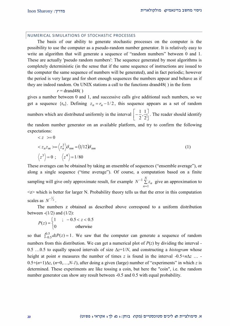
NUMERICAL SIMULATIONS OF STOCHASTIC PROCESSES
The basis of our ability to generate stochastic processes on the computer is the
possibility to use the computer as a pseudo-random number generator. It is relatively easy to
write an algorithm that will generate a sequence of “random numbers” between 0 and 1.
These are actually 'pseudo random numbers': The sequence generated by most algorithms is
completely deterministic (in the sense that if the same sequence of instructions are issued to
the computer the same sequence of numbers will be generated), and in fact periodic; however
the period is very large and for short enough sequences the numbers appear and behave as if
they are indeed random. On UNIX stations a call to the functions drand48( ) in the form
r = drand48( )
gives a number between 0 and 1, and successive calls give additional such numbers, so we
get a sequence {rn}. Defining 2/1 nn rz , this sequence appears as a set of random
numbers which are distributed uniformly in the interval 1 1
,2 2
. The reader should identify
the random number generator on an available platform, and try to confirm the following
expectations:
80/1;0
121
0
43
2
zz
zzz
z
nmnmnmn (1)
These averages can be obtained by taking an ensemble of sequences (“ensemble average”), or
along a single sequence (“time average”). Of course, a computation based on a finite
sampling will give only approximate result, for example
N
nnzN
1
1 give an approximation to
<z> which is better for larger N. Probability theory tells us that the error in this computation
scales as 1
2N
.
The numbers z obtained as described above correspond to a uniform distribution
between -(1/2) and (1/2):
otherwise0
5.05.0;1)(
zzP
so that
5.05.0
1)(zdzP . We saw that the computer can generate a sequence of random
numbers from this distribution. We can get a numerical plot of P(z) by dividing the interval -
0.5 …0.5 to equally spaced intervals of size z=1/N, and constructing a histogram whose
height at point n measures the number of times z is found in the interval -0.5+nz … -
0.5+(n+1)z, (n=0,…,N-1), after doing a given (large) number of “experiments” in which z is
determined. These experiments are like tossing a coin, but here the "coin", i.e. the random
number generator can show any result between -0.5 and 0.5 with equal probability.

Inon Sharony: מדריך ניסוי מחשב בדינאמיקה מולקולארית
12 (המהלך האקראי הפשוט: מקרה בוחן)תהליכים סטוכסטיים יתסימולצי .א
GENERATING PSEUDO-RANDOM NUMBERS FROM A GENERAL DISTRIBUTION
As said above, most computers provide calls to functions which generate pseudo-
random numbers r in the interval 0…1, and by simple shift and scaling we can get random
numbers distributed evenly in any interval (i.e. if r is distributed evenly in the interval [0,1],
then z=(B-A)r+A is distributed evenly in the interval [A,B]). In many applications we want to
generate random numbers whose distribution is other than uniform. For example, in order to
assign velocities to atoms in a molecular system at thermal equilibrium we need to generate
random numbers distributed according to the Maxwell-Boltzmann distribution,
2222/3)2/(exp)/(2),,( zyxzyx vvvmmvvvP . The following theorem from
probability theory provides a useful method:
Let r be a random variable that is distributed uniformly in the interval 0,…,1. Let W(x) be
a nonzero function in the interval bxa , which satisfies 1)(
b
axdxW
. The random
variable z, obtained from r using the relation
z
azWdzr )'('
[namely use this relation to
find z = z(r)], is distributed with the probability density: W(z)dz in the interval bza .
The proof is simple: start from
dzzWdrzWdz
dr)( i.e.;)( (2)
Together with the general relation dzzPdrrP zr )()( between the probability distributions of
random variable r and another such variable z, obtained from r by the 1:1 mapping z=z(r), we
find
)()()( zPzWrP zr (3)
Hence )()( zWzPz (because 1)( rPr (משל) ( .
For example, if r is distributed uniformly in 0,…,1 and z is defined in the interval 0… by
)1()(i.e.;1'
0
' rnrzeedzr
zzz
(4)
then the resulting z is distributed in 0…∞ according to zz ezP )( .
Inon Sharony: מדריך ניסוי מחשב בדינאמיקה מולקולארית
11 (המהלך האקראי הפשוט: מקרה בוחן)תהליכים סטוכסטיים יתסימולצי .א
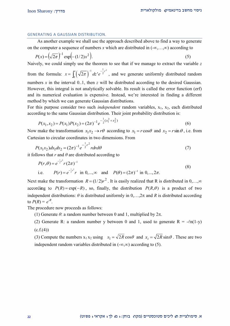
GENERATING A GAUSSIAN DISTRIBUTION.
As another example we shall use the approach described above to find a way to generate
on the computer a sequence of numbers x which are distributed in (-,…,) according to
21)2/1(exp2)( xxP
. (5)
Naively, we could simply use the theorem to see that if we manage to extract the variable z
from the formula: 21
1 '2
02 '
zz
x dz e
, and we generate uniformly distributed random
numbers x in the interval 0..1, then z will be distributed according to the desired Gaussian.
However, this integral is not analytically solvable. Its result is called the error function (erf)
and its numerical evaluation is expensive. Instead, we’re interested in finding a different
method by which we can generate Gaussian distributions.
For this purpose consider two such independent random variables, x1, x2, each distributed
according to the same Gaussian distribution. Their joint probability distribution is:
)(1
2121
22
212
1
)2()()(),(xx
exPxPxxP (6)
Now make the transformation rxx 21 according to cos1 rx and sin2 rx , i.e. from
Cartesian to circular coordinates in two dimensions. From
rdrdedxdxxxPr 2
2
1
12121 )2()(
(7)
it follows that r and θ are distributed according to
1 2
2
1 2
2
1
1
( , ) (2 )
i.e. ( ) in 0,..., and ( ) (2 ) in 0,...,2 .
r
r
P r e r
P r e r P
(8)
Next make the transformation 2)2/1( rR . It is easily realized that R is distributed in 0,…,∞
)exp()( RRP , so, finally, the distribution ),( RP is a product of two
independent distributions: θ is distributed uniformly in 0,…,2 and R is distributed according
to P(R) = e-R
.
The procedure now proceeds as follows:
(1) Generate θ: a random number between 0 and 1, multiplied by 2.
(2) Generate R: a random number y between 0 and 1, used to generate R = -n(1-y)
(c.f.(4))
(3) Compute the numbers x1 x2 using cos21 Rx and 2 2 sinx R . These are two
independent random variables distributed in (-∞,∞) according to (5).

Inon Sharony: מדריך ניסוי מחשב בדינאמיקה מולקולארית
12 (המהלך האקראי הפשוט: מקרה בוחן)תהליכים סטוכסטיים יתסימולצי .א
In summary, the desired random numbers are obtained by generating two random numbers r1
and r2 from a uniform distribution in (0,1), and using them to form
)2sin()1(2
)2cos()1(2
22/1
12
22/1
11
rrnx
rrnx
(9)
Note that the Gaussian distribution that was generated in this way is characterized by <x> = 0
and <x2> = 1. The most general form of a Gaussian distribution is
2
2
1 ( ) 1( ) exp
2 2
yP y
(10)
For which <y> = and <y2> =
2. Random numbers y characterized by such a distribution
can be obtained from the numbers x of (9) using the transformation y = x+.
Yet another method of generating Gaussian distributions is by generating a series of random
variables, and calculating the average of the sequence: 1
1 N
k
k
y xN
, the central limit theorem
in statistics guarantees that for N the random variable y will have a Gaussian
distribution.
We’ve seen three ways to generate Gaussian distributions:
1) Calculating the error-function and inverting it.
2) Generating pairs of random variables.
3) Using the central limit theorem.
What are the advantages and disadvantages of each method?

Inon Sharony: מדריך ניסוי מחשב בדינאמיקה מולקולארית
11 (המהלך האקראי הפשוט: מקרה בוחן)תהליכים סטוכסטיים יתסימולצי .א
APPENDIX: HOW DOES DRAND48() WORK?
drand48() generates double-precision pseudo-random numbers that are uniformly distributed
in the interval [0..1], using a linear congruent algorithm and 48-bit integer arithmetic. It has
an internal buffer, in which it stores a 48-bit integers Xk (smaller then 2.8*1014
). Double
precision floating-point numbers between 0 and 1 are obtained from this 48-bit integer by
dividing the result by the maximal integer 248
-1. Each time drand48() is called, it generates a
new 48-bit integer Xk+1 to replace the last one by:
48
1 mod 2k kX aX c
(mod stands for modulus, which is the reminder in the division of two integers).
The values of the parameters a and c can be set by lcong48(), and the initial number X0 (also
called the random seed) has to be set by srand48() or seed48(). If these values are not
initialized, they assume the following default values:
a=25214903917
c=11
These numbers guarantee that the periodicity of drand48() would be very large, and that the
correlation between elements in the series would be small.
Note that while the first few moments and correlations of the pseudo-random number series
seem to indicate that it’s uncorrelated, some higher moments show that there is some
correlation, and that more complicated methods are needed to create better pseudo-random
numbers.
Bonus: How would the sequence generated by drand48() be affected by the following
changes,
I. Change a to 4
II. Change a to 224
III. Change c to 0
These changes can be effected by use of the lcong48() function.
Inon Sharony: מדריך ניסוי מחשב בדינאמיקה מולקולארית
12 (המהלך האקראי הפשוט: מקרה בוחן)תהליכים סטוכסטיים יתסימולצי .א
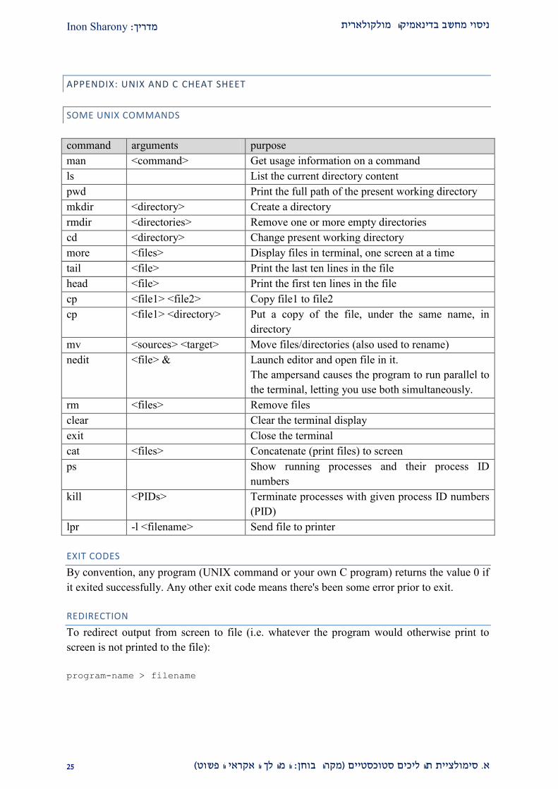
APPENDIX: UNIX AND C CHEAT SHEET
SOME UNIX COMMANDS
command arguments purpose
man <command> Get usage information on a command
ls List the current directory content
pwd Print the full path of the present working directory
mkdir <directory> Create a directory
rmdir <directories> Remove one or more empty directories
cd <directory> Change present working directory
more <files> Display files in terminal, one screen at a time
tail <file> Print the last ten lines in the file
head <file> Print the first ten lines in the file
cp <file1> <file2> Copy file1 to file2
cp <file1> <directory> Put a copy of the file, under the same name, in
directory
mv <sources> <target> Move files/directories (also used to rename)
nedit <file> & Launch editor and open file in it.
The ampersand causes the program to run parallel to
the terminal, letting you use both simultaneously.
rm <files> Remove files
clear Clear the terminal display
exit Close the terminal
cat <files> Concatenate (print files) to screen
ps Show running processes and their process ID
numbers
kill <PIDs> Terminate processes with given process ID numbers
(PID)
lpr -l <filename> Send file to printer
EXIT CODES
By convention, any program (UNIX command or your own C program) returns the value 0 if
it exited successfully. Any other exit code means there's been some error prior to exit.
REDIRECTION
To redirect output from screen to file (i.e. whatever the program would otherwise print to
screen is not printed to the file):
program-name > filename

Inon Sharony: מדריך ניסוי מחשב בדינאמיקה מולקולארית
19 (המהלך האקראי הפשוט: מקרה בוחן)תהליכים סטוכסטיים יתסימולצי .א
SOME C COMMANDS AND EXAMPLES
"FOR" LOOP
int i,max=3;
for(i=0;i<max;i++){
/* do something "max" times*/
printf("For the %d-th time, Hello World!\n",i);//this line prints
"Hello World!" to screen
}
ARRAYS
int i,asize=4;
double a[asize]={0};//note that in C, the array goes from zero to asize-1
for(i=0;i<asize;i++){
a[i]=i*i;
printf("The %d-th component of the array is: a[%d]=%f\n",i,i,a[i]);
}
FILE MANIPULATION
#include <stdio.h>
/*this program reads in 10 lines from input.txt (line-by-line) and writes
them to output.txt, while searching the input for integers and printing
them to screen. The program assumes no line is more than 256 characters
long*/
#define MaxBufferSize 256
#define MaxLines 10
int main(){
FILE *readFP=NULL, *writeFP=NULL;
int i,j=0;
char buffer[MaxBufferSize];
readFP=fopen("input.txt","r");
if (NULL == readFP){
fputs("Couldn't open input.txt for reading. Exiting.\n",stderr);
exit(1);//exit with code 1 (not 0)
}
writeFP=fopen("output.txt","w");
if (NULL == writeFP){
fputs("Couldn't open output.txt for writing. Exiting.\n",stderr);
exit(2);
}
for(i=0;i<MaxLines;i++){
fgets(buffer,MaxBufferSize,readFP);//read a single line from input.txt
and put it in the "buffer" variable
sscanf(buffer,"%d",&j);//scan for the first integer found
printf("In the %d-th line\nthere appears the number %d\n",i,j);
fputs(buffer,writeFP);//write to output.txt
}
return 0;//successful completion
}

Inon Sharony: מדריך ניסוי מחשב בדינאמיקה מולקולארית
12 (המהלך האקראי הפשוט: מקרה בוחן)תהליכים סטוכסטיים יתסימולצי .א
ARITHMETIC, COMPARISON, LOGICAL, AND CASTING OPERATIONS
operator purpose notes
+ addition Binary operator: adds value to its right with
value on its left
- subtraction
* multiplication
/ division Gives integer part in division of integers
% modulus Gives remainder in division of integers
== check equality returns 1 if true, 0 if false
>= check greater than or equal
to
<= check less than or equal to
! negation "not"
&& conjunction "and"
|| disjunction "or"
(int) cast to integer type Changes value to its right to an integer,
discarding the non-integer part (i.e. rounds
down)
(double) cast to double type Changes value to its right to a double

Inon Sharony: מדריך ניסוי מחשב בדינאמיקה מולקולארית
12 (המהלך האקראי הפשוט: מקרה בוחן)תהליכים סטוכסטיים יתסימולצי .א
GNUPLOT – A LINUX GRAPHING TOOL
You may choose to graph your data on another PC, but if you don't, you can use the
GNUPlot program, called by the command gnuplot from the terminal. This program is also
well documented. Information regarding any command can be accessed using the "help"
command. To quit gnuplot just type quit (or use the shortcut command, q).
PLOTTING TO SCREEN
set term x11
set output
# The pound sign (hash) signifies that this is a comment line
# 2-D plot command
plot "data.dat" using 1:2 with lines title "column 2 vs. 1"
# 3-D plot command
splot "data.dat" using 1:2:3 title "3 vs. 2 & 1"
PLOTTING TO FILE
set term jpeg
set output "data.jpeg"
# We can use variables, too
DataFile="data.dat"
abscissa=2
ordinate=3
set xrange [-5.3:16.8]
# p, u, w and t are shortcuts for plot, using, with and title
# The C function sprintf can be used to create formatted text
# We can plot two series of data on a single plot
p DataFile u abscissa:ordinate w linespoints t sprint("%d vs.
%d",ordinate,abscissa), 'data2.dat' u 4:ordinate t "now vs. 4"
FITTING DATA TO A FUNCTION
f(x,y,a,b)=a*cos(x)+b/y
a=5
# fitting parameters initially equal 1 unless specified
fit f(x,y,a,b) 'data.dat' using 1:2 via a,b
Inon Sharony: מדריך ניסוי מחשב בדינאמיקה מולקולארית
12 (המהלך האקראי הפשוט: מקרה בוחן)תהליכים סטוכסטיים יתסימולצי .א
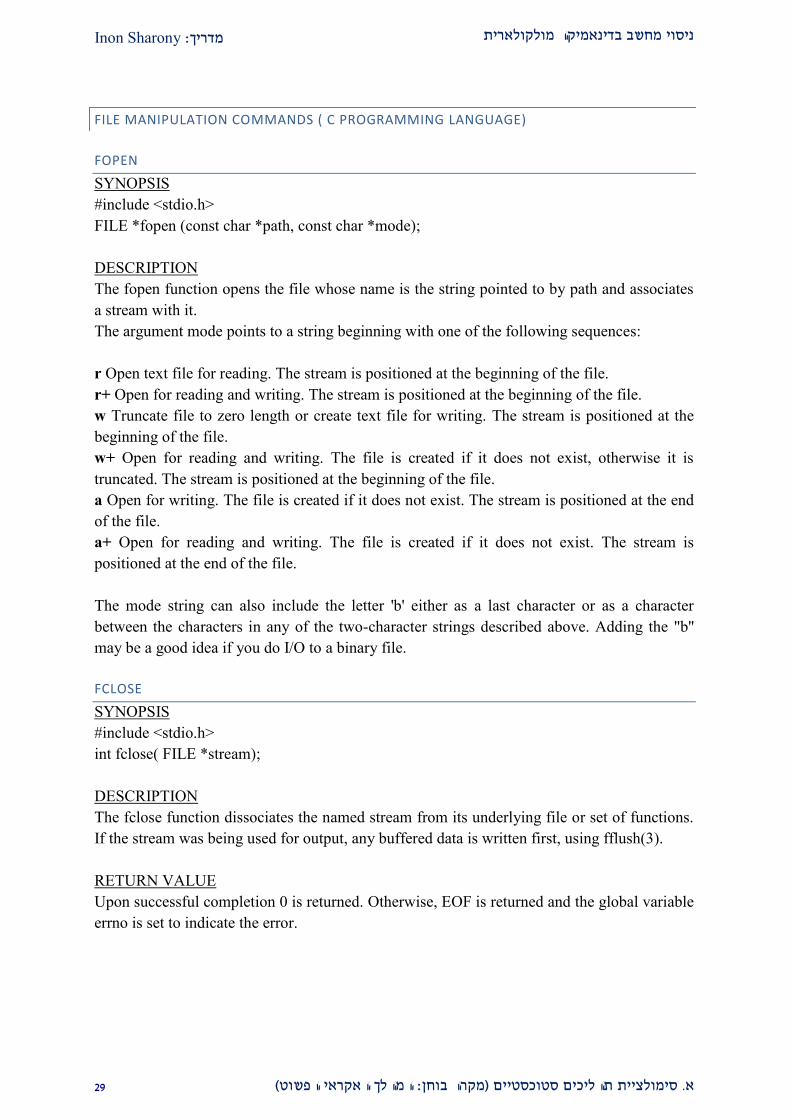
FILE MANIPULATION COMMANDS ( C PROGRAMMING LANGUAGE)
FOPEN
SYNOPSIS
#include <stdio.h>
FILE *fopen (const char *path, const char *mode);
DESCRIPTION
The fopen function opens the file whose name is the string pointed to by path and associates
a stream with it.
The argument mode points to a string beginning with one of the following sequences:
r Open text file for reading. The stream is positioned at the beginning of the file.
r+ Open for reading and writing. The stream is positioned at the beginning of the file.
w Truncate file to zero length or create text file for writing. The stream is positioned at the
beginning of the file.
w+ Open for reading and writing. The file is created if it does not exist, otherwise it is
truncated. The stream is positioned at the beginning of the file.
a Open for writing. The file is created if it does not exist. The stream is positioned at the end
of the file.
a+ Open for reading and writing. The file is created if it does not exist. The stream is
positioned at the end of the file.
The mode string can also include the letter 'b' either as a last character or as a character
between the characters in any of the two-character strings described above. Adding the "b''
may be a good idea if you do I/O to a binary file.
FCLOSE
SYNOPSIS
#include <stdio.h>
int fclose( FILE *stream);
DESCRIPTION
The fclose function dissociates the named stream from its underlying file or set of functions.
If the stream was being used for output, any buffered data is written first, using fflush(3).
RETURN VALUE
Upon successful completion 0 is returned. Otherwise, EOF is returned and the global variable
errno is set to indicate the error.

Inon Sharony: מדריך ניסוי מחשב בדינאמיקה מולקולארית
20 (המהלך האקראי הפשוט: מקרה בוחן)תהליכים סטוכסטיים יתסימולצי .א
FREAD, FWRITE
SYNOPSIS
#include <stdio.h>
size_t fread( void *ptr, size_t size, size_t nmemb, FILE *stream);
size_t fwrite( const void *ptr, size_t size, size_t nmemb, FILE *stream);
DESCRIPTION
The function fread reads nmemb elements of data, each size bytes long, from the stream
pointed to by stream, storing them at the location given by ptr.
The function fwrite writes nmemb elements of data, each size bytes long, to the stream
pointed to by stream, obtaining them from the location given by ptr.
FSEEK
SYNOPSIS
#include <stdio.h>
int fseek( FILE *stream, long offset, int whence);
DESCRIPTION
The fseek function sets the file position indicator for the stream pointed to by stream. The
new position, measured in bytes, is obtained by adding offset bytes to the position specified
by whence. If whence is set to SEEK_SET, SEEK_CUR, or SEEK_END, the offset is
relative to the start of the file, the current position indicator, or end-of-file, respectively.
FPRINTF
SYNOPSIS
#include <stdio.h>
int printf(const char *format, ...);
int fprintf(FILE *stream, const char *format, ...);
DESCRIPTION
The functions in the printf family produce output according to a format as described below.
The function printf writes output to stdout, the standard output stream; fprintf writes output to
the given output stream.

Inon Sharony: מדריך ניסוי מחשב בדינאמיקה מולקולארית
22 (המהלך האקראי הפשוט: מקרה בוחן)תהליכים סטוכסטיים יתסימולצי .א
ח מכין"דו
.ח המכין"שאלות ההכנה ואת פרק הביצוע טרם תחילת כתיבת הדוכל את , קראו את קריאת החובה
Cתכנות בסיסי בשפת .2
פנו אל , LINUXבסביבת או קומפילציה שלו Cבמידה ואינכם שולטים בכתיבת קוד .א .מיד עם קבלת תדריך זההמדריך
תוצאות שהוגרלו N ומציגה, N, המקבלת מספר שלם מהמשתמש Cכתבו תכנית קצרה ב .ב (. 2,1,2,1,2,9סיכויים שווים לקבלת )באקראי בהטלת קובייה
.והגישו את הקוד ופלט לדוגמה, בצעו קומפילציה והרצה לבדיקת תקינותה (2)
והשתמשו בה להצגת ,היסטוגרמה מנורמלתהמייצרת כתבו פונקציה (1)
עבור תוצאות הטלת הקובייה( binsאו , עמודות)היסטוגרמה בת שש מחלקות
.(N >> 1עבור ). המטלות הבאות אין צורך לזכור את כלל המספרים שהוגרלו לשם ביצוע
עדכנו את ההיסטוגרמות ו, מספר יחידהגרילו . אתחלו את ההיסטוגרמות :הדרכה .פעמים Nעל שתי הפעולות האחרונות חזרו . בהתאם למספר שהוגרל
משאבי הזיכרון והן בהיבט צריכת צריכתהן בהיבט , תשפרו את יעילות הקוד כךהניסוי תיווכחו שברובם המכריע של המשך ב. (זמן הריצה)משאבי החישוב
.קודמיםחישובים תוצאות שובים שתבצעו אינם תלויים בזכירת חי, המקרים
?המשתמעת מההיסטוגרמה צפיפות ההסתברותמה ערכי (א)
וכעת ציירו , אותן תוצאות הטלת קובייהחזרו על התהליך עבור (ב) .הציגו פלט לדוגמה .(לבחירתכם) שלוש מחלקות/שתייםהיסטוגרמה בת
מהירויות של , לדוגמה)תבצעו היסטוגרמות של גדלים שאינם שלמים כאשר
תצטרכו להחליט בין כמה עמודות בהיסטוגרמה לחלק ( חלקיקים בקופסהלחלק את תחום bins או" מחלקות"לכמה , בדוגמה שלנו)את התחום
אבל מספיק , פשוטהמקרה של קובייה בעלת שש פאות (. המהירויות הנרמול: להמחשת ההשפעה של מספר המחלקות על ההיסטוגרמה שתיוצר
. של ההיסטוגרמה מושפע גם מגודל התחום התורם לכל אחת מהמחלקות .coarse-graining ייצוג מספר דגימות תחת מחלקה אחת נקרא
והסבירו את ההבדלים חמש מחלקותהיסטוגרמה בת עבור וחזר (ג) .הציגו פלט לדוגמה .ות ההסתברותבהסתברות ובצפיפ
את יצוכעת הר. seedעם אותו ערך עבור ה , הריצו את התכנית פעמיים (2) מה ההבדל. בין הריצה הראשונה לשנייה seedאך שנו את ה , התכנית פעמיים
?בתוצאות
חסכוני יותר להשתמש בקבצים בינאריים במקום , בעבודה עם כמויות גדולות של מידע .גקובץ בינארי הוא קובץ שלא ניתן . רות שלא ניתן לקרוא אותם כטקסטלמ, קבצי טקסט
.וזאת ניתן רק על ידי הכרת התוכנית שכתבה אותו, לקרוא אותו ללא הכרת מבנהו
משלושה ( struct)שמורכב כמבנה dvectorבשם הגדירו סוג משתנה חדש (2) (.double)מספר עשרוני בדיוק כפול כל אחד מהם , רכיבים
(http://www.tau.ac.il/~physchem/Dynamics/code/C/typedefs.h: וראו)
nכתבו פונקציה הכותבת מערך של ו fwriteהשתמשו בפונקצית הספרייה (1) nאחד מ כל : שימו לב שהמערך יהיה מסדר שני .לקובץ בינארי dvectorמשתני
.מספרים 3nכ "סהוב, האיברים מורכב משלושה רכיבים
שלשות nכתבו תכנית הקוראת ו freadהשתמשו בפונקצית הספרייה (2)מחשבת את המנה של , dvectorמשתני nשל מקובץ בינארי לתוך מערךמספרים
מנת לע םהקודשכתבתם בסעיף ראשון בשני ומשתמשת בפונקציה רכיב ההבצעו .לקובץ בינארישל הראשון בשני והמנה השניו ראשוןההרכיב לכתוב את .הגישו את הקודו, והרצה לבדיקת תקינותהקומפילציה

Inon Sharony: מדריך ניסוי מחשב בדינאמיקה מולקולארית
21 (המהלך האקראי הפשוט: מקרה בוחן)תהליכים סטוכסטיים יתסימולצי .א
הקוראת איבר נתוןפונקציה וכתבו fseekהשתמשו בפונקצית הספרייה (1)השתמשו בפונקציה זו . ומדפיסה את תוכנו למסך כטקסטמהקובץ הבינארי
.כטקסטלמסך י מהקובץ הבינאר להדפסת כל איבר שני
וסטטיסטיקה הסתברות .1
מה הקשר למציאת ?יום-איך ניתן לראות זאת בחיי היום? חוק המספרים הגדוליםמהו .אהמוגרל מספר דגימות הולך וגדל של משתנה עבור תנו תיאור כללי ? ערך ממדידה
.אקראית מהתפלגות אחידה
מה הקשר להערכת ?יום-איך ניתן לראות זאת בחיי היום? משפט הגבול המרכזימהו .במספר דגימות הולך וגדל של משתנים עבור תנו תיאור כללי? שגיאה סטטיסטית במדידה
.2aו aיות אחידות ממורכזות בעלות רוחב אקראית מהתפלגו יםהמוגרל
מה ההסתברות לקבל במדידה יחידה ערך השונה ביותר מאחוז מערך התוחלת של .גמה לגבי הממוצע של שתי ?עבור שתי מדידותו ?1ל 1-משתנה המתפלג באופן אחיד בין
ממוצע מה הסיכוי לקבל , (כל אחד)אם נעשה שני ממוצעים על שתי מדידות ?המדידות ?השונה ביותר מאחוז מערך התוחלת של ממוצעים
?"ביצוע הניסוי"של 2תצפו לראות בסעיף מגמהאיזו .2
, התפלגות מספר אקראישל nמנט ה את הביטוי האנליטי לשגיאה במוהביעו .1 nx ,ןבהינת
x, רזולוציית המדידה של המספר . השגיאה היחסית עבורזרו ח.
שאלות בונוס
"(השיכור מהלך) אקראי ומהלך תההסתברו לתורת מבוא"את קריאת הרשות קראו .2
בין המהלך האקראי המיקרוסקופי לבין תופעת הדיפוזיה הקשרהסבירו את .אצפיפות ההתפלגות של משוואת השוו בין : הדרכה? (ללא זרם קבוע)המקרוסקופית
.ההסתברות שמתקבלת מהמהלך האקראי לבין זו של צפיפות החומר בדיפוזיה
( דיפוזיה של חלקיק בתוך נוזל של אותם חלקיקים)מית העריכו את מקדם הדיפוזיה העצ .בבטאו התוצאה . המהלך החופשי הממוצע ומשך המהלך החופשי הממוצעבאמצעות אורך
.והטמפרטורה( חתך פעולה קלסי)שלו רדיוס וה מסת החלקיק, הנוזלבאמצעות צפיפות
ק וטמפרטורה "גרם לסמ 2.221בצפיפות מקדם הדיפוזיה העצמית של ארגון העריכו את .ג .השוו לתוצאה ניסיונית מהספרות עבור צפיפות וטמפרטורה דומותו קלווין 21.1
.נגסטרםוא 2.22, השתמשו ברדיוס ואן דר וולס של ארגון
(התומךקראו את חומר הקריאה ) עוד הסתברות .9
צפיפות ההסתברות וההסתברות ,בין פונקצית ההסתברותהמתמטי מה הקשר .א ? המצטברת
?ההסתברות וצפיפות ההסתברות שוותמתי .ב
?בין קומולנט למומנט ותקשרמשוואות המה ןמה? קומולנטמהו .ג
.כלשהו למומנט יוצרתה פונקציהה ביןקשר הו, התפלגות של יוצרת פונקציהמהי הגדר .ד
איך ניתן לראות ? לורנציאניתמה ניתן לומר על שני המומנטים הראשונים של התפלגות .ה ?לוונציאנישל תהליך ות רבותמדידמהערך שיתקבל ,אם כך, ומה ?יום-זאת בחיי היום
, 1/80שווה ל 1/2ל 1/2-הוכח שהמומנט הרביעי של משתנה שהתפלגותו אחידה בין .ו .זוגיים שלו שווים אפס-ושכל המומנטים האי
?regression analysisמהו ? מה הקשר בין סטטיסטיקה להסתברות .ז

Inon Sharony: מדריך ניסוי מחשב בדינאמיקה מולקולארית
22 (המהלך האקראי הפשוט: מקרה בוחן)תהליכים סטוכסטיים יתסימולצי .א
?(confidence interval) סמך-מרווח ברמהו .ח
מעשנים נמוכה 20,000מחקר טוען שמנת המשכל הממוצעת של קבוצה בת (2)מה הסיכוי שבקבוצה כלשהי . שאינם מעשנים 20,000בשבע נקודות מקבוצה בת
מנת המשכל הממוצעת ( מבלי לדעת אם מי מהם מעשנים)אנשים 20,000בת נת הבהירו את כל ההנחות שעשיתם לגבי התפלגות מ? (22או ) 202תהיה .המשכל
עם תנורמאליבהינתן שעבר האוכלוסייה הכללית מנת המשכל מתפלגת (1)מנת המשכל N מה הסיכוי שעבור מדגם סופי בגודל, וסטיית תקן μ ממוצע
ועבור ( חיובי x ניתן להניח ש)פתרו עבור המקרה הכללי ? x הממוצעת תהיה .=16 ו μ =100 המקרה בו
אם נתון , (covariance)שווה לשונות המשותפת ( correlation)הסבירו מדוע הקורלציה .ט .שהשונות של כל אחד מהמשתנים מוגדרת ואינה אפס
?(OTF)האופטית פונקצית התמסורתל שלההמתמטי מה הקשר? point spread function (PSF)מהי .2 .הקונבולוציהמושג לבין PSFן ה נסחו את הקשר המתמטי בי
םסימולציית תהליכים סטוכסטיי .2
?מה ניתן לעשות כדי שההבדל יהיה זניח? רנדומי מרנדומי-ופסיאודבמה שונה מספר .א
להגרלת היתרונות והחסרונות של כל אחת מהשיטות הבאות של השוואה טבלת ערכו .ב :(גאוסית/ התפלגות פעמון ) נורמאליתמספרים שייצרו התפלגות
.והיפוכה error functionחישוב (2)
-Boxטרנספורם ) קראיים מהתפלגות אחידההגרלת זוגות של משתנים א (1)
Muller).
.משפט הגבול המרכזישימוש ב (2)
מערכת פתוחה למעבר אנרגיה מאופיינת על ידי טמפרטורה הקובעת את אופן החלפת .גלשימור !( לא דטרמיניסטי) סטוכסטיאלגוריתם הציעו . האנרגיה בין המערכת לסביבה
.עם סביבה בטמפרטורה נתונהטמפרטורה עבור חלקיק חופשי שמחליף אנרגיה
שווה לקורלציה הצולבת ( auto covariance)העצמית הסבירו מדוע השונות המשותפת .דמדוע ו ,סטציונארייםעבור תהליכים ממשיים ו( auto cross correlation)העצמית
( cross correlation)קורלציה הצולבת תמונת הראי של השווה ל( convolution)הקונבולוציה . כאלהר תהליכים בוע
!פרטו כאן על מנת לזכות בבונוס, (הכנה או ביצוע)אם גיליתם טעויות בפרק זה של התדריך .2

Inon Sharony: מדריך ניסוי מחשב בדינאמיקה מולקולארית
21 (המהלך האקראי הפשוט: מקרה בוחן)תהליכים סטוכסטיים יתסימולצי .א
ביצוע הניסוי
מספר הואהפלט שלו . ()drand48הוא UNIXבמערכות Cבשפת ( רנדומיים)יוצר המספרים האקראיים .ופן אחידפלגים באתהמשימוש חוזר בו מניב מספרים ו, 2 -ל 0בין אקראי
של ההתפלגות האחידה מומנטים .2
כלומר , האחידה הרנדומית ההתפלגותשל חשבו את שלושת המומנטים הראשונים .א :חשבו
n
1
1 r
N n
n jj
m rN
כאשר 1
N
j jr
10,100,1000,10000N ו,אקראיים היא סדרה של מספרים .
, הציגו את הפיזור הסטטיסטי: וב כל אחד מהמומנטיםבחיש( precision) הדיוקאת חשבו .ב .עבור כל אחד מגדלי המדגמים(N) כלומר סטיית התקן
Nעבור לחישוב האנליטיביחס תוצאות של ה( accuracy) הנכונותהשוו את .ג ,
1לפיו 2 3
1 1 1
2 3 4m m m . בטאו את השגיאה המוחלטת( )יחסית או השגיאה ה
( ,מבוטאת באחוזים.)
11 1 1
0 0 0
1 0 1 1
1 1 1 1
nn n
n
rm r P r dr r dr
n n n n
והפיקו ,Welchשל t מבחן ההתאמהוו את הדיוק והנכונות באמצעות חישוב הש .ד
:משמעויות
.הסבירו ?מתקבלות באופן מגמתי השגיאות הקטנות ביותרעבור איזה מומנט .1
לבין אלו שניתנו ' א 2כלומר ההפרש בין הגדלים שנמדדו בשאלה , N)ציירו את השגיאה היחסית .2עבור שלושת המדגמים ), N, ונקציה של מספר הדגימותכפ( מחולק בגדלים הנתונים', ב 2בשאלה
הציגו את התוצאות עבור שלושת המומנטים כשלוש . עבור כל אחד מהמומנטים, (הגדולים יותרבצעו התאמה לפונקציה ו, תולוגריתמי תבסקאלוסדרות נתונים על גבי גרף יחיד בעל צירים
.שנראית כקו ישר על גרף זה
.צית התאמה זוהסבירו מדוע נבחרה פונק .א האורדינאטהעם ציר ( בלבד)שנקודת החיתוך של סדרת המדידות עבור המומנט הראשון שימו לב
אומד השגיאה הסטטיסטית הנו סטיית התקן של ההתפלגות , עבור מדידה יחידה: ידועה לנו ההתאמה רק עבור פונקציתהיא פרמטר חופשי של האורדינאטהנקודת החיתוך עם , לכן. שנדגמה
.המומנטים הגבוהים יותר
?המתקבלהקו שיפוע מה .ב

Inon Sharony: מדריך ניסוי מחשב בדינאמיקה מולקולארית
22 (המהלך האקראי הפשוט: מקרה בוחן)תהליכים סטוכסטיים יתסימולצי .א
יש צורך להוסיף C -שבשימו לב . ) re, לווחשבו את האקספוננט ש, r ,איהגרילו מספר אקר .1לינק לספריית ,"lm-" הלשם כך ויש להוסיף לפקודת הקומפילצי "<include <math.h" תלתוכני
עבורעבור האקספוננט והראו ש 2 ילתרגחיזרו על (. קההמתמטי
1 1
exp
1 expdzdr
z r
P z dz P r dr dr P z r z
מתקיים
1
exp 1
0 1 1
1 1
ez r e n n nn n
n
z r
z e em z P z dz z z dz
n n n n
. ,קטע מסויםמב שימור ההסתברותמנובעת האמצעית שורה ה
.שיטת ההיפוךבעלי התפלגות כללית נקרא אקראיים טכניקה זו להגרלת מספרים
ההתפלגות ממספרים רנדומיים שמגרילה כתבו תכנית ו Box-Muller טרנספורםהשתמשו ב .2 .(2ושונות 0ממוצע )הנורמאלית הסטנדרטית
מוגדר שפשוט zמדוע משתנה .א21
2r
z e
( עםr לתרגיל בדומה , מוגרל מהתפלגות אחידה ?מתפלג בולצמניתלא (2
.עבור המספרים שהגרלתם מההתפלגות הנורמאלית 2 ילחזרו על תרג .ב
.ציירו היסטוגרמה וודאו באופן איכותי שמתקבלת צורה המתאימה להתפלגות נורמאלית .ג
י"מוגדרת ע rj , ri המשתנים האקראייםשני הקורלציה בין .9
222 2
i j i jij
ij
i ji i j j
rr r r
r r r r
:שלכם RNG -ה בדקו את. חסרי קורלציהיוצר מספרים הוא שהוא טוב RNGל ןקריטריו
אם .א 1
N
j jr
, RNG ה י"ע שנוצרה אקראיים מספרים של סדרה היא
1 הצולבתשונות תא חשבו
1
N k
k i i kN k iC rr
.
1lim ש הראוו, k של כפונקציה Ck את הציגו ,N של םערכי כמה עבור .ב4k
NC
כל עבור k
.השואפים לאחד N/k ערכיקורה עבור מההסבירו .הואש
0ijלדרישה אקוויוולנטיתמדוע תוצאה זו .ג ?
הגרילו סדרה של מספרים אקראיים ושימרו אותה במערך .2 1
N
j jr
חשבו את סדרת הממוצעים .
עבור תוצאות האנליטיות והשוו ל 2 -ו 2 תרגילחזרו עבורם על .qj = ( rj + rj+1 ) / 2: הבאיםשל , השקול לגבול של מגדם אינסופי, הציגו את חישובכם האנליטי :דרכהה) .המשתנים החדשים
(kהמומנטים השונים ושל השונות הצולבת כפונקציה של
בונוסתרגיל
המשפט , להזכירכם)השוו את קצב ההתכנסות של ההתפלגויות לצפי על פי משפט הגבול המרכזי .2ציירו את הגרף של , עבור כל התפלגות: הדרכה(. של המומנט הראשון בלבד להתכנסות סמתייח
ג ובצעו התאמה לפונקציה אנאליטית שנראית לו-השגיאה המוחלטת כנגד גודל המדגם על גרף לוג .הסבירו( ?מי הכי קרוב למינוס חצי)השוואה בין השיפועים טבלת כעת ערכו . כקו ישר על גרף זה
. 2r בתוך ריבוע בעל צלע rניתן לחסום מעגל ברדיוס: בשיטת הזריקה חישוב הערך של .24r שטח הריבוע
2r ושטח המעגל
גם תימצא בתוך הריבוע רה באקראי שנבחההסתברות שנקודה . 2 . /4בתוך המעגל היא
של נקודות בתוך y וה x ה תקואורדינאטושל זוגות מספרים שיהוו ( N) הגרילו מספר גדול .א . r=1ריבוע בעל
(. הרדיוסכלומר את )חשבו את מרחק הנקודה שהוגרלה ביחס לראשית , עבור כל נקודה .ב

Inon Sharony: מדריך ניסוי מחשב בדינאמיקה מולקולארית
29 (המהלך האקראי הפשוט: מקרה בוחן)תהליכים סטוכסטיים יתסימולצי .א
.Mם אשית הגדילו את המספר השלמהר 2מ אם הנקודה נמצאת במרחק הקטן .ג
N עבור /4 יישאף ליחס( "acceptance ratio"או" יחס הקבלה"נקרא גם ה)M/N היחס .ד
. ∞ N בגבול 4M/Nכ ניתן לחלץ את ערכו של. השואף לאינסוף
מכיוון שהיא שקולה לזריקת חצים "rejection method"או " שיטת הזריקה"שיטה זו נקראת
(darts) מטרה בצורת מעגל החסום בריבוע וספירת כלל האבנים שנפלו בתוך הריבועלעבר (N)
משתמשים בשיטה לחשב גם . תוך ההנחה שהפיזור אחיד בכל התחום, (M)ובתוך המעגלועם גבולות אינטגרציה מורכבים יותר מאלו של , אינטגרלים מורכבים יותר מחישוב השטח
.האלמנט הרנדומי הכרוך בהעקב " מונה קרלו"והיא נקראת גם , מעגל
מהלך השיכור .20
בכל צעד זמן : בממד אחד כתבו תוכנית המבצעת סימולציה של מהלך אקראי סימטרי .אאחרת , המערכת נעה צעד אחד ימינה, q = 0.5מ אם המספר גדול. r, מוגרל מספר
.שמאלה
?הממוצע ו המיקוםמה .שרטטו גרף של מיקום המערכת כפונקציה של הזמן .ב
נסו לבצע התאמה . ריבוע המרחק שעברה המערכת כפונקציה של הזמןרף של שרטטו ג .ג תהפיזיקאליהמשמעות הציגו את משוואת הפונקציה והסבירו את , לפונקציה אנליטית
.המופיעים בה של כל אחד מהפרמטרים
ההסתברות למצוא את שרטטו היסטוגרמה של , עבור מסלול בעל מספר רב של צעדים .דהציגו את משוואת , נסו לבצע התאמה לפונקציה אנליטית .P(x), יםמסוהמערכת במקום
מקיימת הראו שהפונקציה האנליטית אותה התאמתם .את תוצאתכם והסבירו הפונקציהאת מספר הקריאות יש לחלק , כדי לקבל הסתברות מנורמלת: הערה. הנרמולאת תנאי
.אבמספר הצעדים הכולל וברוחב התבכל תא
Mהריצו )צעדי זמן Nלמשך תלויים-בלתי מהלכים אקראיים Mל בצעו סימולציה ש .הההיסטוגרמות Mומצעו את , בכל פעם seedכאשר אתם משנים את ערך ה פעמים
השוו בין ההיסטוגרמה . צעדי זמן MxNכעת בצעו סימולציה אחת באורך (. המתקבלותקחו )צעדים MxNמהלכים לבין ההיסטוגרמה עבור המהלך האחד שעבר Mהממוצעת על
?מה המסקנה(. N=2M=100או N=M=100לפחות
?qאם נשנה את ערכו של תשתנה תשובתכם לכל אחד מהסעיפים הקודמים כיצד .ו

Inon Sharony: מדריך ניסוי מחשב בדינאמיקה מולקולארית
22 (המהלך האקראי הפשוט: מקרה בוחן)תהליכים סטוכסטיים יתסימולצי .א
על ידי מתן האפשרות drand48, יוצר המספרים האקראייםשולטת בהגדרות lcong48הפונקציה .22הפונקציה . אקראי הבא-אודופסלקבוע את הקבועים במשוואת הרקורסיה המייצרת את המספר ה
משוואתואת הפרמטרים של ( או הזרע)המגדיר את המספר האקראי הקודם , מקבלת מערך כקלטמאפסת את ()seed48או ()srand48קריאה לפונקציה (. במשוואה בחומר הרקע c -ו a)הרקורסיה
. ()lcong48השינויים שערכה
, אקראי הבא-ן ייצור המספר הפסאודוניתן לשנות את אופ ()lcong48הראו שבאמצעות .א .לנבא את המספרים הבאים ברצףואף
:םרנדומאליי-הדגימו פונקציות נוספות לייצור מספרים פסאודו .ב
-מחזירה מספר פסאודו( ()srandom, ויוצר הזרע המתאים) ()randomהפונקציה (2) .RAND_MAXאקראי שלם בין אפס לקבוע
בייטים אקראיים בפורמט $NUMירה מחז openssl rand –hex $NUM הפקודה (1) .זרע אקראישמחוללים , את הזרע היא לוקחת מקובץ או מחומרה. הקסאדצימלי

Inon Sharony: מדריך ניסוי מחשב בדינאמיקה מולקולארית
22 (תנועה בפוטנציאל הרמוני: מקרה בוחן) קה ניוטוניתמכאני יתסימולצי. ב
(תנועה בפוטנציאל הרמוני: מקרה בוחן) קה ניוטוניתמכאני יתסימולצי. ב
בשלב זה של הניסוי
.דינאמיקה של מערכת במרחב הפאזה רלתיאומשוואות המילטון להשתמש בתלמדו .2
, (קידום בזמן/פרופגציה) אינטגרציה נומרית של משוואות התנועה של ניוטון לבצעמדו תל .1 .יחידות מצומצמותבו velocity Verletאלגוריתם להשתמש ב
ונות תכותכירו דוגמאות ל, םחלקיקיקלאסית של מערכת ה סימולצי מרכיביה שלתלמדו מהם .2 .הניתן לחלץ מתוצרישפיזיקאליות
והפקת תוצאות מהנתונים, פתרון משוואות התנועה של אוסילטור הרמוניתיישמו את שלמדתם ל .1 .מולקולת החנקןתנודות לגבי
קריאהחובת
Chemical Dynamics in"בספר ( 1Aוהנספח ) 2.1 פרק משנהניקה סטטיסטית אמבוא למכקראו .2
Condensed Phases" מאת ניצן. 2. Gould & Tobochnik, "Appendix 3A: Numerical solution of Newton's equations" in An Introduction to
Computer Simulation Methods, Third edition, Pearson (2007).
.בעמודים הבאיםפשוטים של נוזלים ריתאת דינאמיקה מולקולייעל סימולצראו ק .24. Daan Frenkel & Berend Smit, "Ch. 2.2.1: Ergodicity" and "Ch. 4: MD" in Understanding Molecular
Simulations, Second Edition, Academic Press (2002).
5. M.P. Allen & D.J. Tildesley, "Appendix B.1: Reduced units" in Computer Simulation of Liquids, Oxford
University Press (1991).
קריאת רשות
1. Daan Frenkel & Berend Smit, "Appendix A: Lagrangian & Hamiltonian" in Understanding Molecular
Simulations, Second Edition, Academic Press (2002).
.שירטוט של רוב התכונות אותן נחשב בפרק זההכוללת של אוסילטור הרמוני Flashאנימציית .1, הסימולציה מתחו את המסה הצידה על ידי גרירתה בעוד כפתור העכבר השמאלי לחוץלהפעלת
.ושחררו

Inon Sharony: מדריך ניסוי מחשב בדינאמיקה מולקולארית
22 (תנועה בפוטנציאל הרמוני: מקרה בוחן) קה ניוטוניתמכאני יתסימולצי. ב
INTRODUCTION TO STATISTICAL MECHANICS WITH A VIEW TO LIQUIDS
Statistical mechanics and statistical thermodynamics are the branches of science which study
the behavior of macroscopic systems as inferred from the microscopic properties of
individual atoms and molecules. One important tool in this investigation is the "molecular
dynamics method" – direct computer simulation of a representative many body system.
Many books and reviews are available on this method. The following is a brief outline. We
assume at the outset that classical mechanics can be used. For simplicity we assume that the
total potential energy U is a sum of two-particle interactions and that the interaction between
any two molecules depends only on the distance between them. The last two assumptions can
be relaxed at the cost of more complex codes.
As an extra simplification step we assume that the molecules are sphero-symmetrical, so the
interaction between two species depends only on the magnitude of their separation. The total
potential energy U is then
N
ji
ijrururuU1
2312 )(...)()( (12)
where u(rij) depends only on the magnitude of the distance ijr
between particles i and j. The
pairwise interaction form (12) is appropriate for "simple" liquids such as liquid argon.
The form of u(r) for electrically neutral atoms can be constructed, in principle, by a
detailed first principles quantum mechanical calculation. Such a calculation is very difficult,
and it is usually sufficient to choose a simple phenomenological form for u(r). The most
important features of u(r) for simple liquids are a strong repulsion for small r and a weak
attraction at large separation. The repulsion for small r is a consequence of the exclusion
principle. The dominant weak attraction at larger r is due to the mutual polarization of each
atom; the resultant attractive force is called the van der Waals force.
One of the most useful phenomenological forms of u(r) is the Lennard-Jones potential
12 6
( ) 4 u r -r r
(13)
The r-6
dependence in (13) is in accordance with theory for induced-dipole/ induced-dipole
interaction. The r-12
dependence is chosen for convenience only. The Lennard-Jones potential
is parameterized by a "length" and an "energy" . σ is a measure of the range of the
potential while ε is associated with the well depth of its attractive part.
It is convenient to express lengths, energy, and mass in units of , , and m, where m is
the mass of the particles. We measure velocities in units of (/m)1/2
and the time in units of
= (m2/)1/2
. The parameters and of the Lennard-Jones potential for liquid argon are /kB
= 119.8 K and = 3.405Å. The mass m of an argon atom is 6.69 x 10⁻²³
gm and hence =
2.17 x 10⁻¹²
sec.
Time propagation is done by solving the Newton's Eq. of motion. An algorithm which is
especially attractive for its intuitive appeal is given by
2
1
1 1
1 ( )
21
( )2
n n n n
n n n n
x x v t a t
v v a a t
(14)
Here a is the acceleration, obtained at each time step from the known force on each particle.
This is the velocity form of the Verlet algorithm.

Inon Sharony: מדריך ניסוי מחשב בדינאמיקה מולקולארית
10 (תנועה בפוטנציאל הרמוני: מקרה בוחן) קה ניוטוניתמכאני יתסימולצי. ב
BOUNDARY CONDITIONS.
A useful simulation must incorporate all the relevant features of the physical system of
interest. Remember that the ultimate goal of our simulations is to obtain estimates for the
behavior of macroscopic systems - systems of the order of N 1023
-1025
particles. In such a
system surface effects on bulk properties are negligible. Consider for example a spherical
bowl containing N molecules. The fraction of molecules near the walls is proportional to the
surface to volume ratio, Nsurface/N ~ (4R2)/(4R
3/3). Since N = (4/3R
3) where is the
density, the fraction of particles near the walls is proportional to N2/3
/N = N-1/3
, a vanishing
small fraction for N 1023
.
In contrast, the number of particles that can be studied in molecular dynamics simulations is
typically 102-10
4, and the fraction of particles near the walls is not small enough to safely
disregard surface effects on bulk properties. Consequently it is not a good idea to do a
simulation of a macroscopic system by placing a small number of particles in a container
with rigid walls, and if we try it we may find that computed bulk properties depend on the
system size, obviously a physically wrong result.
There is another numerical drawback to simulating molecular motion in a box with rigid
walls: the strong sudden forces exerted by such walls cause errors in the numerical
integration. To see it consider a particle reaching the wall. The numerical code will examine
the position of the particle, and if it finds that under the current integration step it has crossed
the wall, it will place it back into the system at a position that is at the same distance from the
wall inside the system. This implies that the particle position and hence its potential energy
(due to interaction with other particles) is changed without any change in its kinetic energy,
so the total energy would not be conserved.
One way to minimize surface effects while simulating the properties of a macroscopic system
is to use periodic boundary conditions. The simulation cell is surrounded by periodically
repeating replicas of itself; each image cell contains the particles in the same relative
positions. When a particle enters or leaves one face of the central cell, the move is
accompanied by an image of that particle leaving or entering a neighboring cell through the
opposite face. The use of periodic boundary conditions implies that particle 1 interacts with
particle 2 in the central cell and with all the periodic replicas of particle 2. However for short-
range interactions, we often adopt the minimum image approximation. In this approximation
particle 1 in the central cell interacts only with the nearest image of particle 2, be it in the
central cell or in one of its replicas. The reader should convince itself that this implies that
when we consider the interaction of particles 1 and 2, only that replica of particle 2 with
separation smaller than L/2 from particle 1 (in each direction) is taken into account. Other
replicas of particles 2 are disregarded in computing the effect of particles 2 on particle 1.

Inon Sharony: מדריך ניסוי מחשב בדינאמיקה מולקולארית
12 (תנועה בפוטנציאל הרמוני: מקרה בוחן) קה ניוטוניתמכאני יתסימולצי. ב
TEMPERATURE
In a system of particles in thermal equilibrium the velocities are distribution according to the
Maxwell-Boltzmann law. Accordingly, each velocity degree of freedom is associated with an
average energy of (1/2)kBT, where kB is Boltzmann constant. Therefore, the average kinetic
energy of an N-particles system in three dimensions at temperature T is
TNkmE B
N
i
iziyixk2
3
2
1
1
222
(15)
The bracket <...> denotes either a time or an ensemble average. Note that the equation (15)
holds only if the motion of the center of mass of the system is zero, otherwise this speed,
which is not part of the kinetic energy that enters into the temperature, should be subtracted
from the speed of each particle.
INTRODUCTION TO STATISTICAL MECHANICS OF LIQUIDS
THIS CHAPTER FOLLOWS D. CHANDLER "INTRODUCTION TO MODERN STATISTICAL MECHANIC" (PP. 188-
209). SEE ALSO: J.P. HANSEN AND I.R. MCDONALD "THEORY OF SIMPLE LIQUIDS".
This chapter introduces the reader to basic concepts in the theory of classical liquids. We
shall limit ourselves only to concepts and methods needed for the rest of our discussion of
dynamical processes in this environment.
At normal temperatures it is safe, for most liquids, to limit our discussion to the
ground electronic state (liquid metals constitute exceptions to this statement). This defines
(using the Born-Oppenheimer approximation) the potential surface on which the atomic
nuclei are moving. Except for liquids with very light nuclei, e.g. liquid H2, He, possibly Ne,
classical mechanics is usually sufficient to describe this nuclear motion.
STATISTICAL MECHANICS OF CLASSICAL LIQUIDS
The microscopic state of a classical system of N atoms is characterized by a point in
phase space, 1 2 1 2( , ) ( , ,... , , ,..., )N N
N Nr p p p p r r r . The classical Hamiltonian is
2
1
( , ) ( )2
NN N Ni
i i
pH r p U r
m
(16)
Where U is the potential energy which depends on the positions of all atoms in the system.
The probability density to find the system at ( , )N Nr p is
( , )
( , )
N NH r pN N e
f r pQ
; ( , )N NN N H r PQ dr dp e (17)
Q is called the partition function. Quantum statistical mechanics modifies this description in
a conceptually important way: Recall that N Ndr dp is obtained from converting a sum over
all values of rN and p
N to an integral, and in doing so we have to use a density of states factor.
A rough argument is as follows: For a 1-dimensional particle in a region xx p the number
of possible states is ,xx p
h
where h is the Planck constant, because a given 'state' (x, px)
can be defined only within a square of area h.

Inon Sharony: מדריך ניסוי מחשב בדינאמיקה מולקולארית
11 (תנועה בפוטנציאל הרמוני: מקרה בוחן) קה ניוטוניתמכאני יתסימולצי. ב
Therefore the density of states for a single 1-dimensional particle is h-1
and for N particles in
3 dimensions it is 1/h3N
. In addition, if all the particles are identical, we have to divide by N!,
so stateE
states
Q e
becomes
( , )
3
1
!
N NN N H r p
NQ dr dp e
N h
(18)
still, the probability density to be at a given phase point is
( )H
N N
N N H
ef r p
dr dp e
(19)
(so that ( ) 1N N N Ndr dp f r p ) and the corresponding probability is ( , ) .N N N Nf r P dr dp
Using Eq. (16) this distribution function can be written as a product of momentum and
position parts
( ) ( ) ( )N N N Nf r p p P r (20)
where
2
2
/ 2
/ 2( )
i
i
i
i
p m
N
p mN
eP
dP e
(21)
is the probability distribution for the momentum subspace, itself separable into a product of
factors associated with individual degrees of freedom
3
1
( ) ( )N
N
i
i
P p
; 2
2
2
/ 21/ 2 / 2
/ 2
( ) 2i
i
i
p mp m
i B
p m
i
ep mk T e
dp e
(22)
and where
( )
( )( )
N
N
U rN
N U r
eP r
dr e
(23)
is the probability distribution to observe system in configuration phase point rN.
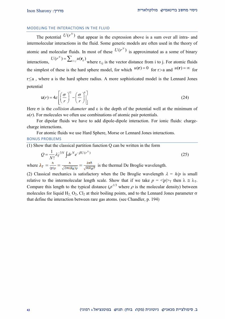
Inon Sharony: מדריך ניסוי מחשב בדינאמיקה מולקולארית
12 (תנועה בפוטנציאל הרמוני: מקרה בוחן) קה ניוטוניתמכאני יתסימולצי. ב
MODELING THE INTERACTIONS IN THE FLUID
The potential ( )NU r that appear in the expression above is a sum over all intra- and
intermolecular interactions in the fluid. Some generic models are often used in the theory of
atomic and molecular fluids. In most of these ( )NU r is approximated as a some of binary
interactions, ( ) ( )N
iji jU r u
r
where ri,j is the vector distance from i to j. For atomic fluids
the simplest of these is the hard sphere model, for which ( ) 0u r for ra and ( )u r for
ra , where a is the hard sphere radius. A more sophisticated model is the Lennard Jones
potential
12 6
( ) 4rr r
u (24)
Here is the collision diameter and is the depth of the potential well at the minimum of
u(r). For molecules we often use combinations of atomic pair potentials.
For dipolar fluids we have to add dipole-dipole interaction. For ionic fluids: charge-
charge interactions.
For atomic fluids we use Hard Sphere, Morse or Lennard Jones interactions.
BONUS PROBLEMS
(1) Show that the classical partition function Q can be written in the form
3 ( )1
!
NN N U rTQ dr e
N
(25)
where is the thermal De Broglie wavelength.
(2) Classical mechanics is satisfactory when the De Broglie wavelength = h/p is small
relative to the intermolecular length scale. Show that if we take p = <|p|>T then T.
Compare this length to the typical distance (-1/3 where is the molecular density) between
molecules for liquid H2, O2, Cl2 at their boiling points, and to the Lennard Jones parameter
that define the interaction between rare gas atoms. (see Chandler, p. 194)

Inon Sharony: מדריך ניסוי מחשב בדינאמיקה מולקולארית
11 (תנועה בפוטנציאל הרמוני: מקרה בוחן) קה ניוטוניתמכאני יתסימולצי. ב
TIME AVERAGE AND ENSEMBLE AVERAGE.
SEE ALSO SUBSECTION 1.4.2 IN NITZAN, AND A MORE VERBAL EXPLANATION IN SUBSECTION 2.2.1 OF
FRENKEL & SMIT.
Consider an equilibrium thermodynamic ensemble, say a set of atomic systems all
characterized by the macroscopic variables T (temperature), V (volume) and N (number of
particles). Each system in this ensemble is a set of N atoms whose positions and momenta are
assigned according to the distribution function (17) subjected to the additional volume
restriction. At a given time each system in this ensemble is in a particular microscopic state
that corresponds to a point ( , )N Nr p in phase space. As the system evolves in time such a
point, together with the Newton's equations of motion, defines a phase space trajectory. The
ensemble corresponds to a set of such trajectories, which, due to the uniqueness of solutions
of the Newton's equations, do not intersect with themselves or with others.
In this microscopic picture, any system property can be described as a function of all
particles positions and momenta, i.e.
( , )N N r p (26)
The associated thermodynamic property is the ensemble average
( ) ( , , )N NA r P A V T N (27)
i.e.
( )
( )
( )( , , ) ( ) ( )
N N
N N
N N H r p N N
N N N N N N
N N H r P
dr dp e r PA V T N dr dp f r p r P
dr dp e
(28)
Eq. (28) defines an ensemble average. Alternatively we could consider defining the
macroscopic thermodynamic property as a time average
0
1( , , ) lim ( ( ) ( ))N NA V T N r t p t dt
(29)
The ergodic theorem states that, for 'realistic' systems, these two kinds of averaging, Eqs.
(28) and (29) yield identical results. For example, if the property under consideration is the
total system's kinetic energy, the corresponding dynamical variable is
2
1
N
i
i
p
; 2 2 2 2
i ix iy izp p p p (30)
Using Eqs. (20)-(22), Eqs (28) and (30) yield
( , , ) 3 BA V T N mNk T (31)
Therefore, Eq. (29) implies that
2 2
1
1 1 1 1lim ( ) lim ( )
3 3
N
i i
iB Bo o
T p t p tmNk mk
(32)
for any atom i. This observation has an important practical consequence: in numerical
simulation we usually follow a single systems trajectory in time. The temperature of the
system can be obtained from such an equilibrium trajectory using Eq.(32). (In practice, the
operation 0
lim(1/ ) d
is replaced by an average over a finite size sampling of points along
the equilibrium trajectory.

Inon Sharony: מדריך ניסוי מחשב בדינאמיקה מולקולארית
12 (תנועה בפוטנציאל הרמוני: מקרה בוחן) קה ניוטוניתמכאני יתסימולצי. ב
THE VIRIAL THEOREM.
The virial function (due to Clausius) is defined by
1
( )N
N
i i
i
r
r F (33)
where Fi is the total force acting on the particle i. Consider the average of this function
1
1lim ( ) ( )
N
i i
io
dt t m t
r r (34)
To evaluate this time average use integration by parts to write
2
0( ) ( ) ( ) ( ) | ( ) |i i i i i
o o
dt t t t t dt t
r r r r r (35)
together with the fact that for a system at finite volume and temperature
1 1
1lim ( ) ( ) (0) (0) 0
N N
i i i i
i i
r r r r
(36)
Using Eqs. (35) and (36) in (34) yields
2
1
1lim | ( ) | 3
N
i B
io
dt m t Nk T
v (37)
The total force, ( )i tF , acting on particle i can be separated into an intrinsic part, arising from
the interaction between particles, and the external part ( )ex
i tF . Consequently
int( ) ( ) ( )N N ex Nr r r (38)
int
1
( ) ( )N
N N
i i
i
r U r
r (39)
If the system is confined to a box of volume V, then, in the absence of additional external
forces, Fex
comes from the pressure exerted on the particles by the wall. In an ideal gas the
inter-particle potential, U(rN), vanishes and the virial function is determined only by this
external force. Therefore
ideal( ) 3 3ex N
Br Nk T PV (40)
It follows that
int1
3BPV Nk T (41)
or
1
1( )
3
NN
B i i
i
PV Nk T U
r r (42)
This is the virial theorem. Conceptually, its importance stems from the fact that it provides an
expression for the pressure as an average of a dynamical variable. On the practical level it
makes it possible for us to calculate the pressure from classical MD simulations.

Inon Sharony: מדריך ניסוי מחשב בדינאמיקה מולקולארית
19 (תנועה בפוטנציאל הרמוני: מקרה בוחן) קה ניוטוניתמכאני יתסימולצי. ב
מכין ח"דו
.ח המכין"שאלות ההכנה ואת פרק הביצוע טרם תחילת כתיבת הדוכל את , קראו את קריאת החובה
משוואות לאינטגרציה של velocity Verletמאלגוריתם יותר יםם פשוטמיאלגוריתם מיהאם קיי .2 .הםחסרונותיהם ויתרונותיאם כן תנו דוגמאות ודונו ב, אם לא הסבירו מדוע? התנועה של ניוטון
, פחות איבריםיהם הם אלה שמופיעים בנוסחאות Verletהאלגוריתמים הפשוטים יותר מ : הערה)יכול להיות tהמיקום בזמן , וגמהלד. ושהפונקציות המעורבות בהם משוערכות בפחות נקודות
(".פשוטה"האפשרות הראשונה היא ה. או בכמה זמנים, tתלוי בפונקציות המשוערכות רק בזמן
שימור אנרגיה .1
פתרון נומרי עבור מערכת שאמורה לשמר גודל מסוים עשוי לשמר את אותו הגודל עד .אמת הדיוק הנדרשת גודלה של שגיאה זו תלוי באלגוריתם ובר. השגיאה הנומרית בלבד
: הדרכה)? עבור פתרון נומרי תנאי מספק לשימור אנרגיהכמה לדעתכם יחשב . ממנו (חישבו על השגיאה היחסית, םפיזיקאלייהשתמשו בשיקולים
משמר יציב ו velocity Verletמדוע אלגוריתם ?יסימפלקטמהו אלגוריתם אינטגרציה .ב ?האנרגיה בדיוק גבו
פרופגציה של שגיאות .2
דיוק להשיג בכדי, המרבי הזמן צעד גודל על התנאי להיות צריך מה איכותי באופן כוהערי .א התדירויות ידי על המאופיינת( לאו דווקא אוסילטור)כללית מערכת של האנרגיה בשימור
שוויון-בטאו את הקשר האיכותי כאי .t משך בעל מסלול לאורך, 2 -ו 1, האופייניות לה .לבין הפרמטרים הנתונים בסעיף זה( ידהמד/וקצב הדגימה) tבין
?תלויהוא הםשב יםנתן השגיאה בגדליבה, השגיאה בגודל תלוימחושבת כיצד .במה הקשר בין גודל אינטרוול הזמן לדיוק במיקום ובמהירות של האוסילטור , לדוגמה
ול בין גודל אינטרווכתוצאה מכך , בין הדיוק במיקום ובמהירות לדיוק באנרגיה, ההרמוני, שאינה משתנה בזמן, על מנת לקבל תלות ממוצעת: הדרכה) ?הזמן לדיוק באנרגיה
עבור אותם גדלים ,כגון הממוצע או שורש ממוצע הריבועים, םאופיינייהשתמש בערכים (התלויים בזמן באופן מפורש
, של האוסילטור ההרמוניעבור שימור אנרגיה של תנאי זההמספרי ערכו את חשבו .ג .ותנאי ההתחלה הנתונים בחלק הביצוע הקודםבסעיף םשהגדרתלפי הרף
תנאי שפה .1
?מהם תנאי התחלה? מהם תנאי שפה .א
? לסימולציה של מערכת מציאותית( תנאי שפה, כלומר)מדוע נדרש תיחום של קופסה .ב ? מה הבעייתיות בהשלכת סימולציה של חלקיק בקופסה קשיחה למערכת מציאותית
.נאי שפהתנו דוגמאות חלופיות לת
מיקום ומהירות כפונקציה של ) לבעיה הפתרון של האנאליטי הביטוי את כתבו, האפשר במידת .2כיצד באה לידי .תוכלו לעשות שימוש בפתרון הספציפי לתנאי ההתחלה שינתנו, בהמשך(. הזמן
?בפתרון הכללי( תנאי התחלה, תנאי שפה, פרמטרים)ביטוי הפיזיקה
הבאים יצוןמקרי הקמה תצפו לקבל עבור .9
∞ ,m0, ∞ ;k 0: של פרמטרים פיזיקאליים .א
: של תנאי ההתחלה .ב
?כיצד נבחר ערכי קיצון, לאו? ניתן לבצע סימולציה של ערך גדול או קטן באופן אינסופי .ג

Inon Sharony: מדריך ניסוי מחשב בדינאמיקה מולקולארית
12 (תנועה בפוטנציאל הרמוני: מקרה בוחן) קה ניוטוניתמכאני יתסימולצי. ב
יחידות מצומצמותמשתנים בעלי .2
? של גדלים הנמדדים ביחידות מצומצמות הממדים והיחידותמהן .א
? g, בתאוצה קבועה hנופל מגובה mמסה על ה גוף בבבמערכת ופייניהזמן האמה .ב ? בסימולציה של מערכת כזו היחידות המצומצמות של הזמןמה יהיו
?בסימולציה נומרית של המערכת צעד הזמןאיזה גודל תבחרו עבור
יחידות מצומצמות להחיל פתרון נומרי משתנים בעלי כיצד מסייע לנו השימוש ב .ג ?גם עבור מערכות בעלות פרמטרים שונים ,שקיבלנו
היחידות : הדרכה) ?בשבוע זהמצמות בהן תעשו שימוש בחלק הביצוע היחידות המצומהן .ד (.ביניהןהאמורה תלות ההמצומצמות של משתנים תלויים יקיימו את
:ההסתברות למצוא את המערכת במצב נתוןו מרחב הפאזהייצוג מצב המערכת ב .2
עליו נשרטט את של מרחב הפאזה צירי הגרףמה הם ? ממדיו הם ומה מהו מרחב הפאזה .א( משתנה) תקואורדינאטמהי ?ממדים dחלקיקים הנעים ב Nבת תנועתה של מערכת
?מרחב הפאזהגרף של כציר ב היחידה שלא מופיעה מרחב-הזמן
כיצד תשתנה התשובה אם מדובר ? מהי הפונקציה המתוארת על גבי מרחב הפזה .בכיצד תשתנה התשובה אם מדובר במערכת יחידה ? יסטית או סטוכסטיתבמערכת דטרמינ ?או בצבר מערכות
תיאור התפתחות המערכת בזמן על גבי מרחב הפאזה .2
?(הגרף תמה צור) במרחב הפאזה במהירות קבועהתנועה של חלקיק תתוארכיצד .א
?של מערכת במרחב הפאזה ההתפתחות בזמןמהן המשוואות המגדירות את .ב
מה הצורה ) במרחב הפאזהחד ממדי אוסילטור הרמוניתנועה של וארתתכיצד .ג, כעת. סמנו את נקודות החיתוך עם הצירים, ראשית: הדרכה ?(שיוצר הגרף תהגיאומטרי
.מצב הקודםב שביקרההתחילו מנקודת חיתוך וחישבו היכן המערכת כהרף עין לאחר
של חלק " ביצוע הניסוי" אי בפרקשאלת המהלך האקרב' לסעיף ה המשפט הארגודימה חשיבות .20הנדרש על מנת לקבל אורך המסלולמה ?בחלק הנוכחי "ביצוע הניסוי"פרק של 2לסעיף ו 'א
?נתוןהאוסילטור בהיסט היסטוגרמה מייצגת של ההסתברות למצוא את
?הטמפרטורה של המערכתוהאם ? קבועה בזמן האנרגיה של מערכת המצומדת לאמבט חוםהאם .22
,טמפרטורות שונותבור ע, העריכו .21
?9-2אילו הבדלים תצפו למצוא בגרפים שמופיעים בתרגילים .א
?"ביצוע הניסוי"של 2בשאלה ' דמה המגמה אותה תצפו לראות בביצוע סעיף .ב .ח המסכם תשוו בין הציפיות שלכם לבין תוצאות הביצוע במעבדה"בדו
שאלות בונוס
(קראו את חומר הקריאה התומך) קצב דגימה .22
?Nyquistתדירות הדגימה של מהי .א
.בחסרונות והשוו השיטותדונו ביתרונות ו? low band pass filterומהו coarse grainingמהו .ב
(קראו את חומר הקריאה התומך) אנליטית וסטטיסטית המכאניקעוד .21
נסחו ביטויים מתמטיים עבור כל ? מהו משפט הויריאליות? מהו חוק החלוקה השווה .א .ו עבור אוסילטור הרמוני קלאסי בממד אחדוהדגימ, אחד מהם
והסבירו (נוזלים תבמכאניקדוגמה וה) Dimensional_Analysisקראו על .ב
principle ofה ערכו השוואה עם ?Rayleigh dimensional analysisמהו (2)
corresponding states שלvan der Waals.
.Gibbsערכו השוואה עם חוק הפאזות של ?Buckinghamשל -משפט ה מהו (1)
אניי'לגרנז פורמליזםעל Daan & Smitשל Aבנספח קראו .ג
?מהו עיקרון הפעולה הסטציונרית? כיצד מוגדרת הפעולה (2)
'?לגראנז-מהן משוואות אוילר (1)
.Noetherשל הראשון שפט ממההראו איך שימור אנרגיה נובע (2)
.יאן'בטאו את הקשר בין ההמילטוניאן ללגרנז ?נדר'מהו טרנספורם לז (1)

Inon Sharony: מדריך ניסוי מחשב בדינאמיקה מולקולארית
12 (תנועה בפוטנציאל הרמוני: מקרה בוחן) קה ניוטוניתמכאני יתסימולצי. ב
פורמליזם ליוביליאני .ד
?מהו הליוביליאן? ליובילו משפט מה (2)
.Liouvilleמאופרטור velocity Verletמשוואות אלגוריתם גזרו (1)
בלתי במה דומה דינאמיקה סימפלקטית של צבר במרחב הפאזה לנוזל וריהסב (2)וכיצד התכונה הסימפלקטית קשורה לשימור המטריקה של , דחיס
(.טרנספורמציה קנונית)מרחב הפאזה קואורדינאטות
מהו מעריך ,של אלגוריתם יציבותכיצד מוגדרת וריהסב, Daan & Smitשל 1פרק על פי .הLyapunov ומה הקשר ביניהם.
תנאי השפה הבאים ותנו דוגמה מחיי רשמו ביטוי מתמטי עבור כל אחד מסוגי :עוד תנאי שפה .22 יום-היום
Dirichlet .א Neumann .ב Robin .ג Cauchy .ד Mixed .ה Born-von Karman (PBC) .ו
:של תנועה במרחב הפזה הופאזאמפליטודה .29
כלומר )ני הקלסי בטאו את הפתרון האנליטי למשוואות התנועה של האוסילטור ההרמו .א .הופאזבאמצעות אמפליטודה ( מיקום כפונקציה של זמן
כיצד מתבטאת התלות באמפליטודה . הביעו את אנרגיית האוסילטור כפונקציה של הזמן .ב .הסבירו? הובפאז
תמולקולארידינאמיקה .22
?מולקולאריתמה מגדיר כוחות קצרי טווח וכוחות ארוכי טווח בדינאמיקה .א
(בחרו, במידה ויש כמה אפשרויות) ביטוי מתמטי לכל אחד מהפוטנציאלים הבאיםכתבו .ב
(2) Bond stretching
(1) Angle bending
(2) Dihedral twisting
(1) Improper torsion
(2) Cross terms
הבאים וכתבו מהכוחות העיקרון הפיזיקאלי מאחורי כל אחדהסבירו במשפט אחד את .ג :ביטוי מתמטי
(2) Coulomb
(1) van der Waals
(2) Keesom
(1) Debye
(2) London
הסבירו ,הבאים ודליםממההסבירו במשפט אחד את העיקרון הפיזיקאלי מאחורי כל אחד .ד :של כל פרמטר בו תהפיזיקאליואת משמעותו עבור הכוח את בחירת הביטוי המתמטי
.מערכת כדורים קשיחים (2)
(תנו דוגמה אחת. )מערכת כדורים רכים (1)
(2) Morse
(1) Lennard-Jones
עבור תכנית דינאמיקה מולקולארית כללית שמקבלת כפרמטרים את תרשים זרימהציירו .ה, פונקצית הפוטנציאל כתלות בקואורדינאטות שלהם, המסות שלהם ,מספר החלקיקים
וכפלט מציגה את המיקומים , את המיקומים והמהירויות ההתחלתיות ואת משך ההרצה .והמהירויות בכל צעד זמן
!פרטו כאן על מנת לזכות בבונוס, (הכנה או ביצוע)אם גיליתם טעויות בפרק זה של התדריך .22
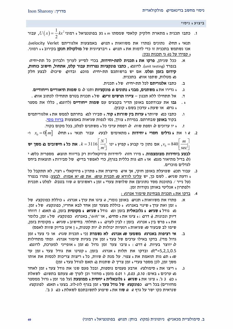
Inon Sharony: מדריך ניסוי מחשב בדינאמיקה מולקולארית
12 (תנועה בפוטנציאל הרמוני: מקרה בוחן) קה ניוטוניתמכאני יתסימולצי. ב
ביצוע הניסוי
הנע בפוטנציאל הרמוני m סי שמסתואנית המתארת חלקיק קלכתבו תכ .2 21
2U x kx , עבור
. (velocity Verletפתרו את משוואות התנועה באמצעות אלגוריתם ) תנאי התחלה נתונים .בקירוב ההרמוני מולקולת חנקןהתנועה הויברציונית של נשתמש בתכנית זו כדי לדמות את אנו
:נכון תכנות נוהגי על הקפידו
יחידה -די לסייע לערוך ולבדוק כל תתבכ, יחידות-פרקו את התכנית לתת, ככל שניתן .א, חישוב כוחות, אתחול, כתבו פונקציות נפרדות עבור קלט, לדוגמה (.unit testing)בנפרד
יחידה מוכנה ובדוקה שיכולה לבצע חלק -אם יש ברשותכם תת. קידום בזמן ופלט .שתפו אותה בתכנית, מהמטלות
.יחידה של התכנית-לכל תת אלגוריתםכתבו .ב
.שמות תיאוריים וייחודייםותנו להם והפונקציות מבני הנתונים ,המשתניםאת הגדירו .ג
.של התכנית בטרם תתחילו לכתוב אותה ציירו תרשים זרימה –אל תתחילו ללא תכנון .ד
כללו את מספר , לדוגמה) שמות ייחודייםבקבצים עם ופן תדיראם בכאת עבודת גבו .ה .(הגרסה או שעת העדכון בשם הקובץ
את האלגוריתמים לממשהסבירו למה בחרתם .הערות בין שורות הקודשיותר כמהכתבו .ו .גומי ברווזלנפות שגיאות באמצעות נסו , במידת הצורך .שבחרתם באופןבקוד
.בכל מקום בקוד, הדפסת ערכי כל המשתנים לפלטל השור פתלהוסערוכים היו .ז
התחלההתנאי עבור בעיההמתאימים ל הגדלים חסרי היחידותזהו את .1 0 0x m ו-
0 840sec
mv
3116נתון כי קבוע הקפיץ הינו אם,
Nk
m
את כל החישובים בהמשך יש .
המירו חזרה ליחידות פיזיקאליות רק בדיווח תוצאה מספרית כלשהי . לבצע ביחידות מצומצמותות ביחס כדי לאפשר בדיקה של סבירות התוצא, (להבדיל מתיאור מגמה או התנהגות כללית בגרף)
.מוכריםלגדלים
לא תתקבל כל , הרצוי יהפיזיקאליצרת את הפתרון אך אינה מי, עבור תכנה שפועלת באופן חוקי .2פתרו בנפרד :עלינו לוודא שהתכנית עושה את שהיא אמורה לבצעיש , לשם כך. הודעת שגיאה
לפלט התכנית בטבלה את שלושת צעדי הזמן הראשונים והשוו( כנת מסד נתוניםובת / על נייר) .ולפתרון האנליטי באותן נקודות זמן
:בדקו את התכנית מבחינת שימור אנרגיה .1
כפונקציה של הכוללת ערך האנרגיה את וגיוהצ, משוואות התנועה באופן נומריאת פתרו .א .כפונקציה של הזמן, מצעד זמן אחד לבא אחריווללת השינוי באנרגיה הכערך ואת הזמן
דווחו ?בהתאמה, בזמן השגיאה המקומית גודל בזמן ומה אליתהשגיאה הגלוב גודל מהכלומר , באנרגיה כפונקציה של הזמן, "drift"או ,הציגו את הסחיפה: הדרכה. )דיוק ונכונות
, בחישוב השגיאה המקומית בזמן .לבין לערכה ההתחלתי tן האנרגיה בזמן את ההפרש בי (בדיוק שוות לאפסהן אינן , קטנות יכולות להיות הרגעיותשימו לב שבעוד שהשגיאות
זמן הצעד כי התכנית שגויה או כי ) אי רציפות באנרגיה משמעו שהאנרגיה לא נשמרת .בבדקו באילו ערכים של צעד הזמן אין בעיות שימור אנרגיה ומתי מתחילות . (גדול מדי
לדוגמה , הציבו צעד זמן גדול מהזמן האופייני למערכת: הדרכה) .להיווצר בעיות
dt*=5,2,1,0.5 הקטינו את גודל צעד הזמן עד . ובדקו את תלות האנרגיה בזמןכל הריצות צריכות לכסות את אותו , על מנת להשוות. שההתנהגות תואמת את הצפוי
(לכן מספר צעדי הזמן צריך להשתנות בהתאם לגודל צעד הזמן, משך זמן
לאחד זמןהצעד גודל ובכל פעם שנו את ,פעמים נוספות ארבעהריצו את הסימולציה .גמזמן המחזור וכן לערך שהצעתם בתשובה לשאלת 0.02ו , 0.02, 0.20 :מהערכים הבאים
על פני זמן הגדול ממספר ) הממוצעתהיחסית הגלובאלית השגיאה הציגו את .'ג 2הכנה בצעו התאמה לפונקציה .לוג-בגרף לוגהזמן פונקציה של גודל צעדכבכל ריצה ( מחזורים
.'ב 2את השיפוע לתשובתכם לשאלת הכנה השוושנראית כקו ישר על גרף זה ו

Inon Sharony: מדריך ניסוי מחשב בדינאמיקה מולקולארית
20 (תנועה בפוטנציאל הרמוני: מקרה בוחן) קה ניוטוניתמכאני יתסימולצי. ב
סימטרי של משוואות התנועה צריך להיות הפתרון , היפוך הזמןב תלוי-בלתיההמילטוניאן מכיוון ש .2 :בדקו זאת. (זוגית בזמןהפתרון הינו פונקציה )גם כן תחת היפוך הזמן
בכל אחד מהסעיפים . ן את גודל השגיאה אך אין חובה להציג את כל המסלוליש לציי: הדרכה) (הבאים יש להשוות את הגדלים בטבלה ולדווח דיוק ונכונות
כך שהיא כעת מהווה תנאי , קחו את הקונפיגורציה האחרונה שהודפסה והיפכו אותה .א
ההתחלה old old new new, 0 , 0x t v t x v צעד הזמן סימנו של היפכו את .:
האם קיבלתם בחזרה כקונפיגורציה אחרונה את תנאי .והריצו את התכנית( )
.הסבירו? יצאתםמהם ההתחלה
ערכה בסוף מינוס לת והחלפת המהירו ,םהחל מהערך הסופי שהתקבל עבור המיקו .ב
,להמסלו old old new new, 0 , 0x t v t x v , נו אמורים א , ןלאחר זמ
לשוב בדיוק אל new old new old0 , 0x t x v t v .
ת רו איהסב, את הגרפים הבאים (ביחידות מצומצמות)ציירו ,נתוניםההתחלה העבור תנאי .9והציגו את משוואת כל ונסו להתאימן לפונקציות אנליטיות הצורות המתקבלות בגרפים השונים
.פונקציה
.על גרף יחידוביחידות מצומצמות , רות כפונקציה של הזמןהמיקום והמהי: הקינמאטיק .אהסבירו מאילו שיקולים פיזיקאליים נובעת כל אחת מהתכונות , הבאים גרףאחד מהעבור כל גבולות , (הםכל אחד מ ויחידות) טווחותחום הגדרה (:במידה והיא רלוונטית)הבאות
.מסלולים סגוריםו( ודות פיתולונק קיצוןנקודות ) סטציונאריותנקודות , ואסימפטוטות
.המיקום כפונקציה של קינטיתהאנרגיה ה .ב
(. xכפונקציה של vx) מסלול במרחב הפאזהה .ג
x.,כלשהו למצוא את החלקיק במקום P(x) ההסתברותצפיפות את הציגו , x(t), עבור מסלול ארוך .2צוא את יש למ, מכיוון שצפיפות ההסתברות להימצא בנקודה מסוימת היא אפסית: הדרכה
חלקו את התחום בו . היסטוגרמהזוהי למעשה . ההסתברות למצוא את החלקיק בתחום מסויםובדקו באיזה חלק של צעדי הזמן נמצא החלקיק בכל , ניתן למצוא את החלקיק למספר מחלקות
ניתן לקרב את צפיפות ההסתברות להסתברות זו כאשר רוחב כל המחלקות . אחת מהמחלקות .יש לנרמל את ההיסטוגרמה (.של המחלקות שואף לאינסוף מספרן)שואף לאפס :P(x)של נובעות כל אחת מהתכונות הבאות שיקולים פיזיקאלייםהסבירו מאילו
.P(x)שבהן משוערכת הפונקציה {{xiנקודות ה .א
.האורדינאטהשל והערכים היחידות .ב
עבור את האינטגרל נומריתחשבו ) .על פני כל התחום P(x) האינטגרל מתחת לפונקציה .ג (ההיסטוגרמה שלכם
.9שאלה עבור הסעיפים האחרונים בהמפורטות ת המתמטיוכל התכונות .ד
:ואנרגיה קינטית טמפרטורה .2
2 "טמפרטורה"חשבו את ה .א /k BT E k מתוך חוק החלוקה השווה) של החלקיק ,
זכרו שעבור מערכת , עם זאת .דווחו הערכת שגיאה, (האנרגיה הקינטית נההי Ek כאשרהמחושבת " טמפרטורה"לכן ל, ת היטבאינה מוגדר" טמפרטורה"ה ,אנרגיההמשמרת .זהה לטמפרטורה הרגילההאין משמעות פיזיקאלית בסעיף זה
שווה לפעמיים האנרגיה הכוללת ממוצע נובע שרמוני ההאוסילטור להויריאלי המשפט מ .בהאנרגיה ו, היא לא משתנה בזמןאזי , אם האנרגיה נשמרת .ממוצע האנרגיה הקינטית
את ממוצע האנרגיה הקינטית לאנרגיה השוו .תההתחלתיהכוללת הממוצעת שווה לזו .הכוללת ההתחלתית
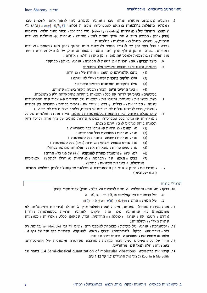
Inon Sharony: מדריך ניסוי מחשב בדינאמיקה מולקולארית
22 (תנועה בפוטנציאל הרמוני: מקרה בוחן) קה ניוטוניתמכאני יתסימולצי. ב
ניתן להפוך אותה לתכנית שבה . התכנית שכתבתם מתארת תנועה שבה האנרגיה נשמרת .2 י "ע( כלומר ) T טמפרטורה נתונהבהתאם ל האנרגיה מתפלגת בולצמנית
מדי פרק זמן הנבחר מתוך חלוקה רנדומית : (velocity rescaling) של המהירויות" התאמה חוזרת" מוחלפת במהירות v(t) המהירות ,(פרק הזמן הממוצע חייב להיות ארוך יחסית לזמן המחזור)
.הבולצמניתמוגרל מההתפלגות שערכה , vT,תרמיתן יש להגריל מספר ולהשוות אותו למשך הזמן מאז התאמת המהירות בכל צעד זמ: הדרכה
להגריל מהירות חדשה יש , במידה והזמן שחלף ארוך יותר מאשר המספר שהוגרל. האחרונה .מונה הזמן מאז ההחלפה האחרונהולאפס את מההתפלגות הבולצמנית
?מבוקשהבאופן אנרגיה דואגת להתפלגות התכנית אכן האם ה כיצד תבדקו .א
:תכננו כיצד תבצעו שינויים אלו לתוכנית, ראשית .ב
.חוזרת של המהירותהלהתאמה אלגוריתםכתבו (2)
?ישתנו ואילו לא ישתנו חלקים בתכניתאילו (1)
?תצטרכוחדשים שתניםומפונקציות אילו (2)
.עבור התכנית לאחר ביצוע השינויים תרשים זרימההציגו (1) .ולא מצומצמות תפיזיקאליוות בסעיפים הבאים יש לדווח את כלל התוצאות ביחיד
ות טמפרטור עבור שתי 6-8תרגילים התוצאות של וחשבו את, בצעו את השינויים, כעת .גנקודות בין ווים המחברים בקאת הגרפים ציירו : הדרכה) .הסבירו את ההבדלים .שונות
(..כלומר בעלי נגזרת לא רציפה ,בכדי להדגיש גדלים לא רציפים או חלקים, השערוךאת ההתפלגויות של כל ציירו .השוואה בין התוצאות בטמפרטורות השונותטבלת ערכו .ד
דיוק ופרטו, בכל טמפרטורה כשלוש סדרות נתונים על גרף אחד המהירויות שהוגרלו :ביחס לגדלים להם הייתם מצפים ונכונות ?המהירויות שהוגרלו בכל טמפרטורה תחוםמה (2) ? בכל טמפרטורה הממוצעתמהי המהירות (1) ?בכל טמפרטורה ביותר השכיחהמהי המהירות (2) ? בכל טמפרטורה (RMS)המהירות וצע ריבועישורש מממהו (1) ?בפועל ות שנדגמיות את ההתפלגווהמתאר ותמה הטמפרטור (2)
?על פני כל התחום P(v) האינטגרל מתחת לפונקציהלמה שווה (9) של התפלגות המהירויות שהוגרלו לפונקציה אנאליטית התאמהבצעו (2)
.והציגו את משוואת הפונקציה, מנורמלת .שלושה ממדיםבבולצמן -להתפלגות מאקסוול תוצאותיכםוהשוני בין הדמיון הסבירו את .ה
(יעקוביאן: רמז)
בונוס יתרגיל
עבור מקרי קיצון( ח המכין"מהדו)בדקו התנהגות הסימולציה בהתאם לציפיות .20
∞ ,m0, ∞ ;k 0: של פרמטרים פיזיקאליים .א
: של תנאי ההתחלה .ב
לא , ביחידות פיזיקאליות)צריך להיות לה היסט התחלתיאיזה , אם המערכת מתחילה ממנוחה .22 ? כדי שהאנרגיה שלה תהיה שקולה לאנרגיה תרמית בטמפרטורת החדר( מצומצמות
האנרגיות הממוצעות , שבאופן כללי ,זכרו .חשבו את האנרגיה הכוללת ההתחלתית: הדרכה) (.שונות מאלו ההתחלתיות
רק , כלומר) semi-log plotהציגו על גבי : אמבט חוםהיסטוגרמת האנרגיה של מערכת המצומדת ל .21. ובצעו התאמה לפונקציה שנראית כקו ישר על גרף זה, (בסקלה לוגריתמית האורדינאטהציר
.ודווחו דיוק ונכונות חלצו מהשיפוע את הטמפרטורה, חזרו על כל הסעיפים לעיל עבור מערכת המורכבת משרשרת אינסופית של אוסילטורים .22
.תנאי שפה מחזורייםהחלת באמצעות
בספר של Semi-classical quantization of molecular vibrations 1.4משנה -קראו את פרק .21Koonin & Meredith שם 2.21עד 2.2ובצעו את תרגילים.
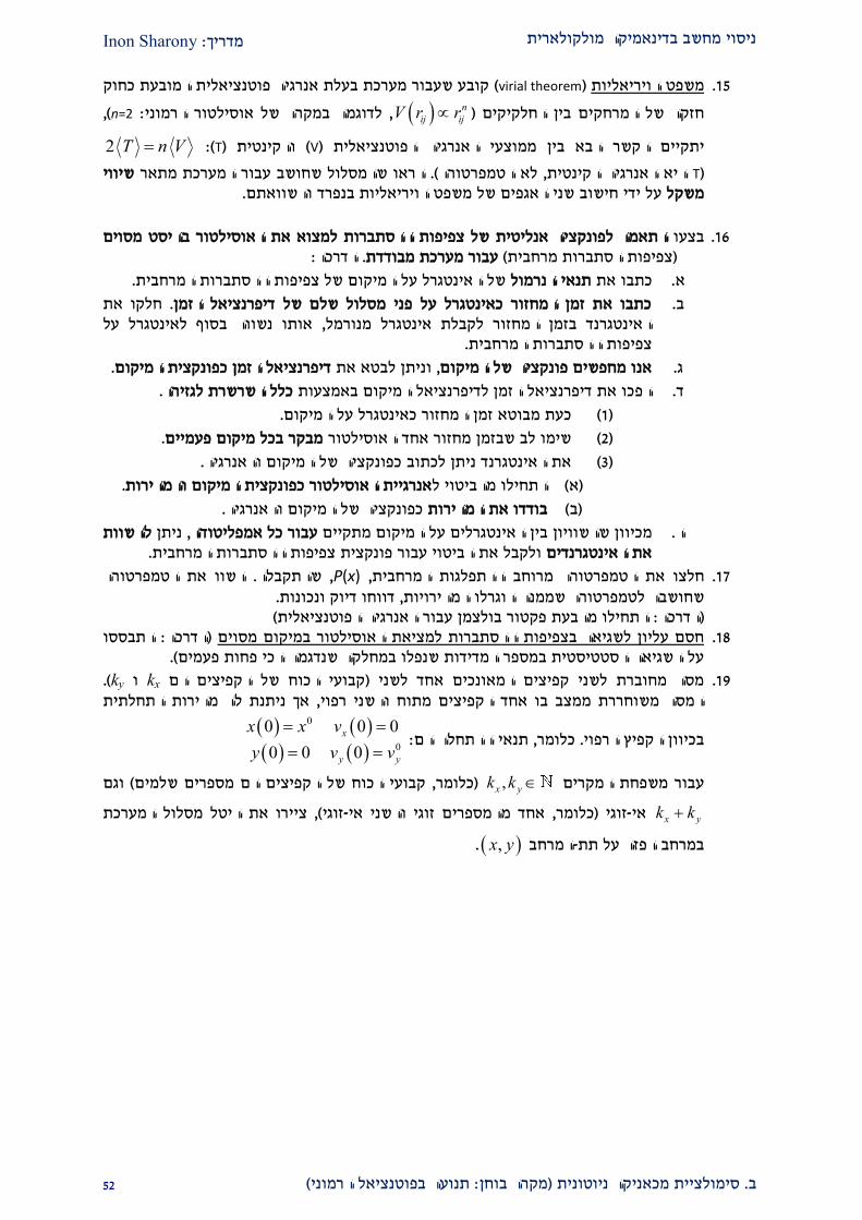
Inon Sharony: מדריך ניסוי מחשב בדינאמיקה מולקולארית
21 (תנועה בפוטנציאל הרמוני: מקרה בוחן) קה ניוטוניתמכאני יתסימולצי. ב
קובע שעבור מערכת בעלת אנרגיה פוטנציאלית המובעת כחוק ( virial theorem) משפט הויריאליות .22
)ים בין החלקיקים חזקה של המרחק n
ij ijV r r ,לדוגמה במקרה של אוסילטור הרמוני :n=2) ,
2(: T)והקינטית (V) הבא בין ממוצעי האנרגיה הפוטנציאלית יתקיים הקשר T n V
(T לא הטמפרטורה, היא האנרגיה הקינטית .)י שיוו מתארמערכת מסלול שחושב עבור ההראו שה .והשוואתם בנפרד משפט הויריאליותשני האגפים של חישוב על ידי משקל
של צפיפות ההסתברות למצוא את האוסילטור בהיסט מסויםלפונקציה אנליטית התאמה בצעו .29 :הדרכה. עבור מערכת מבודדת (צפיפות הסתברות מרחבית)
.מרחביתההסתברות השל האינטגרל על המיקום של צפיפות הנרמולתנאי תבו את כ .א
חלקו את . כתבו את זמן המחזור כאינטגרל על פני מסלול שלם של דיפרנציאל הזמן .באותו נשווה בסוף לאינטגרל על , האינטגרנד בזמן המחזור לקבלת אינטגרל מנורמל
.צפיפות ההסתברות המרחבית
.המיקוםת דיפרנציאל הזמן כפונקציוניתן לבטא את , אנו מחפשים פונקציה של המיקום .ג
.כלל השרשרת לגזירהכו את דיפרנציאל הזמן לדיפרנציאל המיקום באמצעות הפ .ד
.כעת מבוטא זמן המחזור כאינטגרל על המיקום (2)
.מבקר בכל מיקום פעמייםשימו לב שבזמן מחזור אחד האוסילטור (1)
.את האינטגרנד ניתן לכתוב כפונקציה של המיקום והאנרגיה (2)
.המיקום והמהירות ציתכפונקאנרגיית האוסילטור להתחילו מהביטוי (א)
.כפונקציה של המיקום והאנרגיה בודדו את המהירות (ב)
להשוות ניתן , עבור כל אמפליטודהבין האינטגרלים על המיקום מתקיים שהשוויוןמכיוון .ה .צפיפות ההסתברות המרחבית פונקציתולקבל את הביטוי עבור את האינטגרנדים
מפרטורה את הטהשוו .שהתקבלה, P(x), ההתפלגות המרחביתרוחב מ את הטמפרטורהחלצו .22 .דווחו דיוק ונכונות, ה שממנה הוגרלו המהירויותטמפרטורשחושבה ל
(פקטור בולצמן עבור האנרגיה הפוטנציאלית תעבמההתחילו : הדרכה)התבססו : הדרכה) מסויםהאוסילטור במיקום חסם עליון לשגיאה בצפיפות ההסתברות למציאת .22
(.על השגיאה הסטטיסטית במספר המדידות שנפלו במחלקה שנדגמה הכי פחות פעמים
(. kyו kxקבועי הכוח של הקפיצים הם )מסה מחוברת לשני קפיצים המאונכים אחד לשני .22התחלתית אך ניתנת לה מהירות , המסה משוחררת ממצב בו אחד הקפיצים מתוח והשני רפוי
: תנאי ההתחלה הם, כלומר. בכיוון הקפיץ הרפוי
0
0
0 0 0
0 0 0
x
y y
x x v
y v v
x,עבור משפחת המקרים yk k (קבועי הכוח של הקפיצים הם מספרים שלמים, כלומר ) וגם
x yk k רו את היטל מסלול המערכת ציי, (זוגי-אחד מהמספרים זוגי והשני אי, כלומר)זוגי -אי
המרחב -במרחב הפזה על תת ,x y.
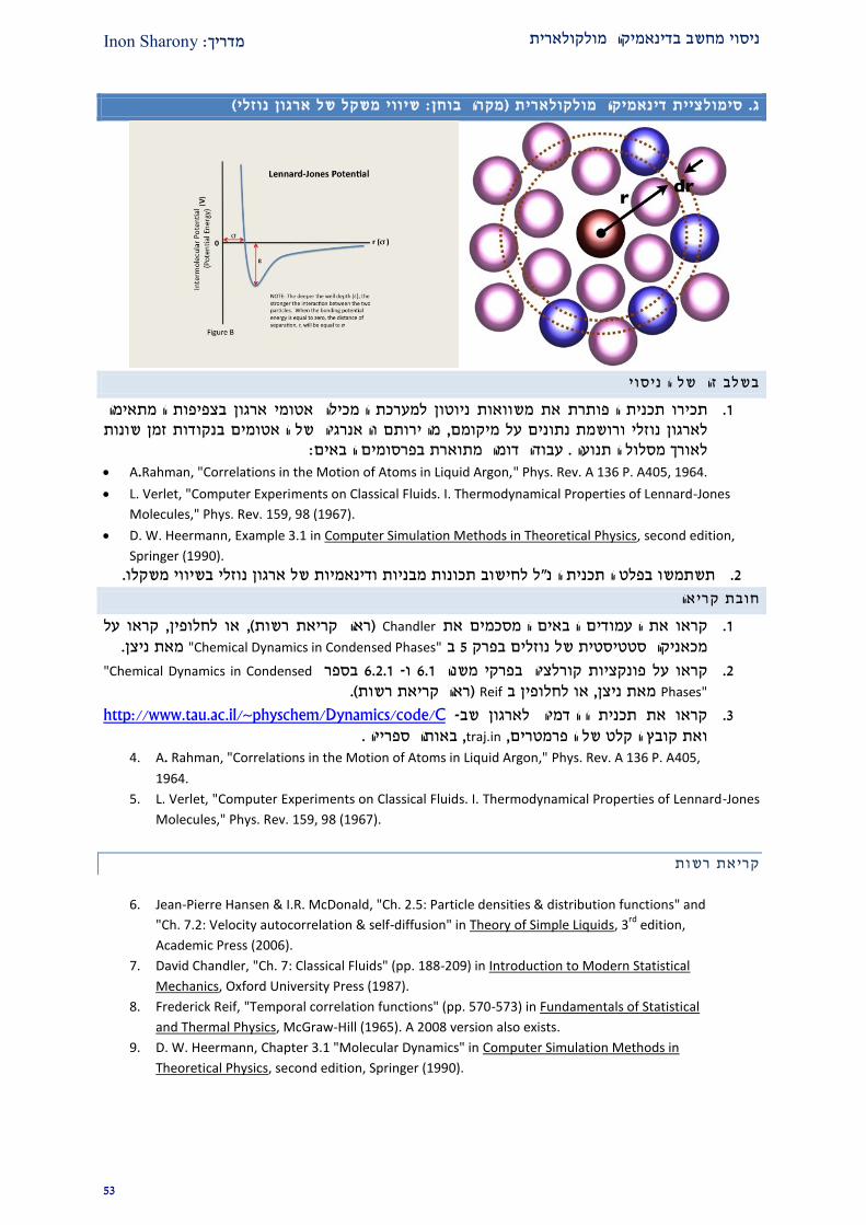
Inon Sharony: ךמדרי ניסוי מחשב בדינאמיקה מולקולארית
22
(נוזלי ארגון של משקל שיווי: מקרה בוחן) מולקולאריתדינאמיקה סימולציית. ג
בשלב זה של הניסוי
פותרת את משוואות ניוטון למערכת המכילה אטומי ארגון בצפיפות המתאימה תכירו תכנית ה .2מהירותם והאנרגיה של האטומים בנקודות זמן שונות , קומםירושמת נתונים על מו נוזלי לארגון
:םהבאי בפרסומיםמתוארת דומהעבודה .לאורך מסלול התנועה A.Rahman, "Correlations in the Motion of Atoms in Liquid Argon," Phys. Rev. A 136 P. A405, 1964.
L. Verlet, "Computer Experiments on Classical Fluids. I. Thermodynamical Properties of Lennard-Jones
Molecules," Phys. Rev. 159, 98 (1967).
D. W. Heermann, Example 3.1 in Computer Simulation Methods in Theoretical Physics, second edition,
Springer (1990).
.בשיווי משקלו שוב תכונות מבניות ודינאמיות של ארגון נוזליל לחי"תשתמשו בפלט התכנית הנ .1
קריאה חובת
קראו על , או לחלופין, (ראה קריאת רשות) Chandlerהעמודים הבאים המסכמים את קראו את .2 .מאת ניצן "Chemical Dynamics in Condensed Phases"ב 2פרק במכאניקה סטטיסטית של נוזלים
Chemical Dynamics in Condensed"בספר 9.1.2 -ו 9.2פרקי משנה ב יהפונקציות קורלצעל קראו .1
Phases" או לחלופין ב , מאת ניצןReif (ראה קריאת רשות.)
e/Chttp://www.tau.ac.il/~physchem/Dynamics/cod -שבקראו את תכנית ההדמיה לארגון .2 .באותה ספרייה, traj.in, של הפרמטריםקלט הקובץ את ו
4. A. Rahman, "Correlations in the Motion of Atoms in Liquid Argon," Phys. Rev. A 136 P. A405,
1964.
5. L. Verlet, "Computer Experiments on Classical Fluids. I. Thermodynamical Properties of Lennard-Jones
Molecules," Phys. Rev. 159, 98 (1967).
קריאת רשות
6. Jean-Pierre Hansen & I.R. McDonald, "Ch. 2.5: Particle densities & distribution functions" and
"Ch. 7.2: Velocity autocorrelation & self-diffusion" in Theory of Simple Liquids, 3rd
edition,
Academic Press (2006).
7. David Chandler, "Ch. 7: Classical Fluids" (pp. 188-209) in Introduction to Modern Statistical
Mechanics, Oxford University Press (1987).
8. Frederick Reif, "Temporal correlation functions" (pp. 570-573) in Fundamentals of Statistical
and Thermal Physics, McGraw-Hill (1965). A 2008 version also exists.
9. D. W. Heermann, Chapter 3.1 "Molecular Dynamics" in Computer Simulation Methods in
Theoretical Physics, second edition, Springer (1990).

Inon Sharony: ךמדרי ניסוי מחשב בדינאמיקה מולקולארית
21
LIQUID PROPERTIES FROM CLASSICAL MOLECULAR DYNAMICS
THIS CHAPTER FOLLOWS DAVID CHANDLER, "CH. 7: CLASSICAL FLUIDS" (PP. 188-209) IN INTRODUCTION
TO MODERN STATISTICAL MECHANICS, OXFORD UNIVERSITY PRESS (1987).
SEE ALSO JEAN-PIERRE HANSEN & I.R. MCDONALD, THEORY OF SIMPLE LIQUIDS, 3RD EDITION,
ACADEMIC PRESS (2006).
This chapter introduces the reader to basic concepts in the theory of classical liquids.
We shall limit ourselves only to concepts and methods needed for the rest of our discussion
of dynamical processes in this environment.
While analytic work is easily done on systems of one extreme or another (e.g. ideal gas,
lattice solid, etc.), liquids pose a challenge in that there are less "small parameters" to derive
solutions to arbitrary precision. For example, a (nearly) ideal gas has low particle density,
yielding a weakly-interacting system (low interaction energies and weak intermolecular
coupling), whereas a lattice solid has high particle density yielding a strongly-interacting
system (high interaction energies, strong intermolecular coupling). We can treat these cases
as two extremes: Nearly-free nuclei, or tightly-bound nuclei (or tight-binding model). While
in the first case entropy is high and processes are entropically driven (dS>0), in the second
case entropy is low and processes are energetically driven (dE<0). Typical time-scales may
be the mean time between collisions in the first kind of systems, and the period of small
vibrations about the configuration of minimum energy in the second kind. Typical length-
scales may be the mean free path in the ideal gas system, and the lattice constant in the
ordered solid. The quantum mechanical description of the system might emphasize localized
wavefunctions in the gas and delocalized wavefunctions in the solid. Liquids are non-trivial
in that none of these limits might be relevant, and we have to deal with more than one scale
for each parameter. We can, however, approximate the behavior of the liquid for short
durations and distances, and build an iterative solution. We will do this numerically.
At normal temperatures it is safe, for most liquids, to limit our discussion to the ground
electronic state (liquid metals constitute exceptions to this statement). This defines (using the
Born-Oppenheimer approximation) the potential surface on which the atomic nuclei are
moving. Except for liquids with very light nuclei, e.g. liquid H2, He, possibly Ne, classical
mechanics is usually sufficient to describe this nuclear motion.
REDUCED CONFIGURATIONAL DISTRIBUTION FUNCTIONS
Consider the configuration space distribution function P(rN). Mathematically, it is the
joint distribution function to find the N particles of the system in their respective positions in
configuration space, i.e. P(rN)dr
N is the probability to find particle 1 in the range dr1 near r1,
and particle 2 in the range dr2 near r2, and particle 3 in the range dr3 near r3, and so on.
We may define a reduced joint distribution function to find the two particles 1 and 2 at
location 1r ,
2r , respectively, irrespective of the positions of all other particles, by
(2 / )
1 2 3 4( , ) ... ( )N N
NP d d d P r r r r r r (43)
Note that both P and P(2/N)
are normalized, i.e.
(2 / )
1 2 1 2( , ) ( ) 1N N Nd d P d P r r r r r r (44)
If all the particles in the system are identical then r1 and r2 could be the coordinates of any
two particles in the system. It is sometimes convenient to use a normalization that will
express the fact that, if we look at the corresponding neighborhoods of r1 and r2, than the

Inon Sharony: ךמדרי ניסוי מחשב בדינאמיקה מולקולארית
22
probability to find these neighborhoods occupied by any two particles increases in a
statistically determined way with the number of particles in the system. This is achieved by
multiplying the joint distribution function (2 / )
1 2( , )NP r r by the number, N(N-1), of distinct
pairs in the system. This yields the pair distribution function
(2 / ) (2 / )
1 2 1 2( , ) ( 1) ( , )N NN N P r r r r . (45)
This concept can be generalized. The reduced joint distribution function for particles 1,...,n is
given by
( / )
1 1 2( ,..., ) ... ( )n N N
n n n NP d d d P r r r r r r (46)
and the n particle distribution function is defined by
( )( / ) ( / )
1 1( )
! !( ,..., ) ( ,..., )
! !
N
N
U rn N n N N n
n nN U r
N N eP d
N n N n dr e
r r r r r (47)
where 1...N n
n Nd dr dr
r . To get a better feeling for these functions it is useful to note that
the relation of (2 / )
1 2( , )N r r to (2 / )
1 2( , )NP r r is the analog of the relation between
(1/ ) /N N V and (1/ ) 1/NP V . The distributions P are normalized to 1 while (1/ )N is
normalized to the number of particles N, (2 / )N is normalized to the number of pairs, N(N-1),
etc.
In an isotropic fluid P(1/N)
does not depends on the particle's position and therefore
(1/ ) 1NP
V ;
(1/ )N N
V (48)
i.e. (1/ )N is just the density ρ. In an ideal gas there are no correlations between particles,
therefore in an isotropic system
(2 / ) (1 / ) (1 / )
1 2 1 2 2
1( , ) ( ) ( )N N NP P P
V r r r r (49)
Hence, the pair distribution function for an isotropic ideal gas is given by
(2 / ) 2
1 2 2
( 1)( , )N N N
V
r r (50)
Correlations in the system caused by deviation from ideality can be measured by the pair
correlation functions
(2 / ) 2
1 2 1 2( , ) ( , ) /Ng r r r r (51)
or
(2 / ) 2
1 2 1 22( , ) ( , ) 1
N
h g
r r r r (52)
It should be intuitively clear that the correlation between any two particles vanishes as
1 2| | r r . Therefore 1g and 0h in this limit. For isotropic fluids
1 2 1 2( , ) (| |)g g r r r r , and similarly for h. In this case we refer to these functions as radial
distribution functions.
The physical meaning of the pair correlation function g can be elucidated by referring to
a mathematical concept from probability theory. Consider a joint probability distribution
function 1 2( , )P x x for two random variables x1 and x2. 1 2 1 2( , )P x x dx dx is the joint probability

Inon Sharony: ךמדרי ניסוי מחשב בדינאמיקה מולקולארית
29
to find the variable x1 in the neighborhood dx1 of x1 and the variable x2 in the neighborhood
dx2 of x2. The reduced single variable distribution functions
1 1 2 1 2 2 2 1 1 2( ) ( , ) ; ( ) ( , )P x dx P x x P x dx P x x (53)
are analogs of the reduced probability distributions defined above, e.g. Eq. (43). Thus,1 1( )P x
is the probability distribution for the variable x1 irrespective of the value assumed by x2. The
conditional probability distribution, 1 2( | )P x x , defined by
1 21 2
2 2
( , )( | )
( )
P x xP x x
P x (54)
expresses something different. 1 2 1( | )P x x dx is the probability that the variable x1 takes a
value in the neighborhood dx1 of x1 given that the other variable has the numerical value x2.
Similarly, 2 1 2 1 2 1 1( | ) ( , ) / ( )P x x dx P x x P x is the probability that the variable x2 takes a value
in the neighborhood dx2 of x2 given that the other variable has the numerical value x1.
In analogy, the single particle conditional distribution function
(2 / )
(1/ ) (2 / )1 21 2 1 1 1 2 1(1/ )
2
( , )( | ) ( , )
( )
NN N
N
PP d d VP d
P
r rr r r r r r r
r (55)
(the second equality holds for an homogeneous fluid) is the conditional probability to find
particle 1 in the neighborhood dr1 of r1 given that particle 2 (or, if all particles are identical,
any particle) is at r2. Using Eqs. (45) and (51) this can be rewritten in the form
(1/ )
1 2 1 2( , ) ( | )Ng NP r r r r (56)
The product on the r.h.s. is the density (number of particles per unit volume) of particles at r1
given that a particle is at r2. Reformulating this for an homogeneous system this gives the
following interpretation of g(r):
ρg(r) is the density of particles at r given that a particle sits at the origin r=0.
If in addition the system is isotropic, g depends only on the modulus r of r. In the absence of
correlations between particles, g=1 and this density is simply ρ irrespective of whether there
is a particle at the origin or not. When correlations do exist g gives important information on
their effect on the fluid structure.

Inon Sharony: ךמדרי ניסוי מחשב בדינאמיקה מולקולארית
22
G(R) CAN BE MEASURED (GENERAL KNOWLEDGE).
For normal liquids the characteristic structural distance is of order ~ 1 Å. A probe of liquid
structure should therefore have a characteristic wavelength in this range. This calls for x-rays
or sub atomic particles. If we want to probe short range structure the use of particles should
be limited to neutral ones, such as neutrons. To see how g can be measured by x-ray or
neutron scattering consider the scheme of a scattering experiment shown in the figure. An
atom at rA scatters an incoming wave with wave-vector kin and the scattered wave with
wave-vector kout is monitored by the detector at RD. The scattering angle is θ, as shown. We
consider elastic scattering only, i.e. in out| | | | k k k .
A
kin
kout
detector(0,0,0)
rA
RD
The scattered wave at the detector is
( )1( )
| |
( )
| |
in A out D A
out D A
i i
D A
i i
D C
S f k e
f ke e
k r k R r
k R k r
R r
R R
(57)
where f(k) is an atomic scattering factor, out in k k k and RC is the center of the scattering
sample. The approximation of replacing rA by RC holds for large distances (relative to sample
size) between system and detector, in which case the positions of all scattering centers
contribute about the same in the denominator. This approximation obviously cannot be
invoked in the exponential terms that determine the phase in the scattered wave. The
appearance in the denominator of the distance between the atom and the detector (all vectors
are related to the origin at (0,0,0)) is due to the fact that the scattered intensity should depend
inversely on this distance.
Since the scattering is elastic (|kin| = |kout|) the scattering angle θ and the modulus of the
scattered wave-vector are associated by
4
2 | | sin sin2 2
ink k
(58)
To obtain the total scattered intensity, the scattered wave, Eq. (57), has to be summed over all
scattering centers and the resulting amplitude should be absolute-squared. The signal at the
detector is thus

Inon Sharony: ךמדרי ניסוי מחשב בדינאמיקה מולקולארית
22
22
21
| ( ) |( ) ( ) ( )
| | | |
out Dj
i Ni
C D j C D
e f kI f k e NS k
k R
k r
R R R R (59)
where S is the structure factor, the factor in I(θ) that depends on the fluid structure:
( )
, 1
1( ) l j
Ni
l j
S eN
k r r
k (60)
To find a more explicit form for S(k) we first separate it to its diagonal (l=j) and non-
diagonal parts. The diagonal part yields 1. In a homogeneous isotropic system all ( 1)N N
non-diagonal terms are identical. We get
1 2( )1( ) 1 ( 1)
iS N N e
N
k r rk
1 2( )( 1)
1
iN U
N U
dr e eN N
N dr e
k r r
1 2( )(2 / )1 2 1 2
11 ( , )
iNd d eN
k r rr r r r (61)
The last equality was obtained using Eqs. (43) and (45). Since the system is homogeneous we
have (2 / ) 21 2 12( , ) ( )N g r r r with 12 1 2 r r r . Therefore the integrand is a function of r12
only and 1 2 12 1 12d d d d V d r r r r r . This yields
1212 12( ) 1 ( )
iS d g e
k r
k r r (62)
This identifies S(k) with the Fourier transform of the pair correlation function, so the latter
may be obtained from the structure factor by inverting the transform. Finally, denoting
12| |r r and using, for an isotropic system, 12( ) ( )g g rr we get
2 cos
0 0
4( ) 1 2 ( ) sin 1 sin( ) ( )ikr
o
S dr r g r d e dr r kr g rk
k (63)

Inon Sharony: ךמדרי ניסוי מחשב בדינאמיקה מולקולארית
22
G(R) CAN BE USED TO CALCULATE THERMODYNAMIC PROPERTIES
Because some of the important interactions used to model atomic and molecular fluids are
binary, the corresponding averages that correspond to macroscopic thermodynamic quantities
can be expressed in terms of the pair correlation function. As an example consider the
average potential energy in a homogeneous atomic fluid of identical particles with
( ) ( )N
ij
i j
U r u r (64)
We already know that the average kinetic energy is (3/2) BNk T , so once the average
potential energy has been calculated we will have a full microscopic expression for the total
system energy. The average potential energy is
12
( 1)( ) ( )
2ij
i j
N NU u u
r r
( )12
( )
( 1) ( )1
2
N
N
N u
N U
N N d u e
d e
r
r
r r
r
2 ( )
1 2 12( )
( 1)( )
2
N
N
N u r
N u r
dr eN Nd d u
dr e
r r r (65)
Using again the definition of the pair correlation function g, this leads to
2 2
1 2 12 12
1 1( ) ( ) ( ) ( ) 2 ( ) ( )
2 2o
U d d g u N d g u N drr g r u r
r r r r r r r (66)
The last equality holds for an isotropic system. This result is intuitively clear: For each one of
the N particles in the system (taken to be at the origin), the potential energy is obtained as a
volume integral, with the integrand being the density of interaction energy involving this
particle. The latter is ρg(r) (density of other particles at position r), multiplied by u(r).
THE REVERSIBLE WORK THEOREM (SEE CHANDLER P. 201)
For an isotropic system at equilibrium (TVN)
( )( ) W rg r e (67)
where W(r) is the change in Helmholtz free energy in a process in which two tagged particles
are brought from infinite separation (in the system) to a relative separation r. By definition,
this is the reversible (minimal) work needed to perform this task.
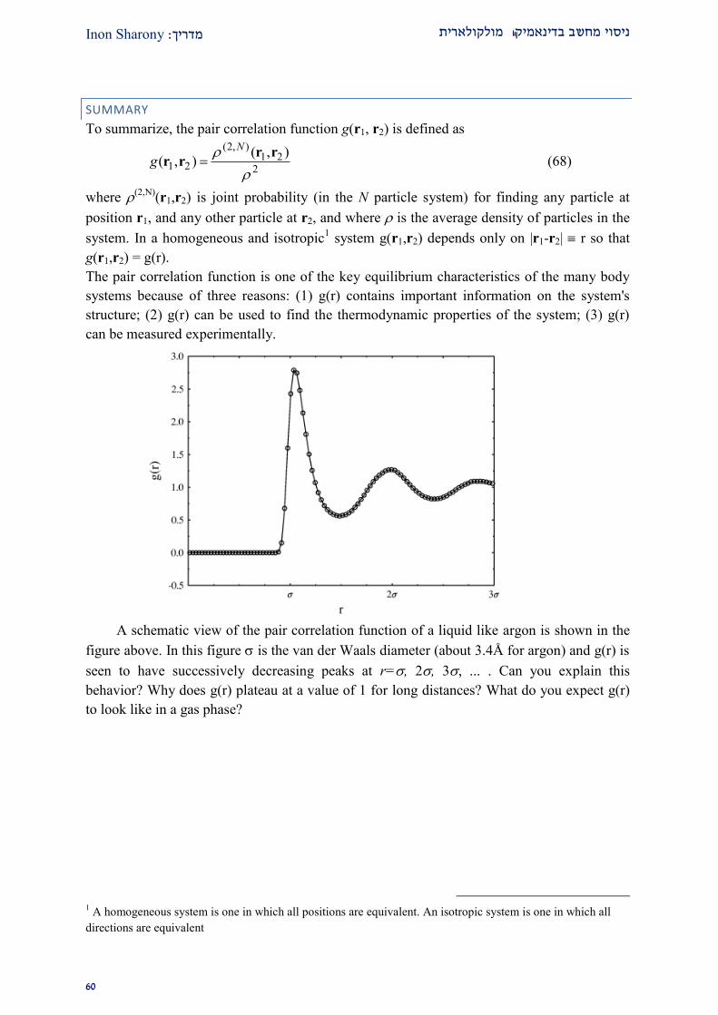
Inon Sharony: ךמדרי ניסוי מחשב בדינאמיקה מולקולארית
90
SUMMARY
To summarize, the pair correlation function g(r1, r2) is defined as
2
21),2(
21
),(),(
rrrr
N
g (68)
where (2,N)(r1,r2) is joint probability (in the N particle system) for finding any particle at
position r1, and any other particle at r2, and where is the average density of particles in the
system. In a homogeneous and isotropic1 system g(r1,r2) depends only on |r1-r2| r so that
g(r1,r2) = g(r).
The pair correlation function is one of the key equilibrium characteristics of the many body
systems because of three reasons: (1) g(r) contains important information on the system's
structure; (2) g(r) can be used to find the thermodynamic properties of the system; (3) g(r)
can be measured experimentally.
A schematic view of the pair correlation function of a liquid like argon is shown in the
figure above. In this figure is the van der Waals diameter (about 3.4Å for argon) and g(r) is
seen to have successively decreasing peaks at r=, 2, 3, ... . Can you explain this
behavior? Why does g(r) plateau at a value of 1 for long distances? What do you expect g(r)
to look like in a gas phase?
1 A homogeneous system is one in which all positions are equivalent. An isotropic system is one in which all
directions are equivalent

Inon Sharony: ךמדרי ניסוי מחשב בדינאמיקה מולקולארית
92
DYNAMICS
Before we leave this introduction to the fluid state we dwell very briefly on dynamical issues.
We will come back to these issues later, and the present discussion is just a demonstration of
the importance of another class of correlation functions - time correlation functions.
We have seen (A. Nitzan, Lecture notes on solids) that for atomic harmonic solids of
identical atoms, the density of modes ρ(ω) is related to the Fourier transform of the velocity-
time correlation function through
( )
(0) ( ) i tmdt t e
N kT
v v (69)
The integrand is related to the velocity autocorrelation function, defined by
( ) (1/3) ( ) (0)C t t v vv . (Note that because of the symmetry in time of the Newton
equations of motion ( ) ( ).C t C t v v ) For an isotropic system this is ( ) ( ) (0)x xC t t v v v
with the x direction chosen at will. This function has the following properties
2
(0)
( ) 0
B
x
k TC
m
C t
ν
(70)
We have argued that Eq. (69) can be used also for liquids for short time scales, i.e. for large
ω. It is indeed plausible that liquids behave as disordered solids on very short time scales. It
is also obvious that this is not the case for long time scales. As a demonstration, consider the
zero frequency component of the correlation function that appears in Eq. (69). For harmonic
solids we have found that this Fourier transform goes to zero in the ω→0 limit like ω2. For
liquids we will now show that the zero frequency component of C(t) is related to the self
diffusion constant of the fluid.
THE DIFFUSION EQUATION.
Consider a fluid made of identical particles that diffuse in space according to the diffusion
equation (Fick's law), namely P(x,t), the probability density to find a particle at point x
satisfies the equation 2
2
( , )( , )
P x tD P x t
t x
(71)
What does this imply for the particle's averaged motion? Suppose the particle starts at the
origin, x = 0. Its average position at time t is given by
( , )tx dxxP x t
(72)
Therefore
2
2( , )
xD dx x P x t
t x
(73)
Integrating the r.h.s by parts, using the fact that P and its derivatives have to vanish at |x|→,
leads to
Inon Sharony: ךמדרי ניסוי מחשב בדינאמיקה מולקולארית
91
0x
t
i.e. 0x at all times. (74)
Consider now the second moment
2 2 ( , )tx dxx P x t
(75)
whose time evolution is given by
2 2
2
2
x PD dx x
t x
(76)
Again, integration by parts of the r.h.s and using the boundary conditions at infinity, i.e.
2
2 2
22 2 2 2
P P Pdx x x dx x xP dxP
x xx
(77)
leads to 2 / 2x t D , therefore, since 2
0 0x ,
2 2tx Dt (78)
For 3-dimensional diffusion in an isotropic system the motions in the x, y and z directions are
independent (the equation ( , ) /P t t r 2 2 2 2 2 2/ / / ( , )D x y z P t r is separable),
so
2 2 2 2 6t t t tr x y z Dt (79)
This is an exact solution of the diffusion equation, regarded as a property of a physical
system it is valid only at long times because the diffusion equation itself holds for such times.
The diffusion coefficient may therefore be calculated from
21
lim | ( ) (0) |6t
D tt
r r (80)

Inon Sharony: ךמדרי ניסוי מחשב בדינאמיקה מולקולארית
92
USE
0
( ) (0) ' ( ')
t
t dt t r r v
This implies
'2
0 0 0 0
| ( ) (0) | ' " ( ") ( ') 2 ' " ( ") ( ')
t t t t
t dt dt t t dt dt t t r r v v v v (81)
The last equality holds because ( ) ( ).C t C t v v Therefore
"
0 0
1lim " ' ( " ')
t t
tD dt dt C t t
t (82)
This can be simplified. Change variable " 't t , with θ goes from "t to 0 and
This yields
0 0
1lim ( ) ( ) ( )
t
tD d t C d C
t
(85)
We found that the self diffusion coefficient is the time integral of the velocity auto-
correlation function!
0
1( ) (0)
3D dt t
v v (86)
"dt d leads to
"
0 0
1lim " ( )
t t
tD dt d C
t
(83)
The integral is done over the shaded area in the
picture. Using this picture it is easily seen that
the order of integration may be changed
according to
0
1lim " ( )
t t
tD d dt C
t
(84)

Inon Sharony: ךמדרי ניסוי מחשב בדינאמיקה מולקולארית
91
REDUCED UNITS IN LENNARD JONES LIQUIDS
The liquid model used is a Lennard Jones liquid, where potential energy is given by a sum of
binary interactions
ji
ijN rurU )(
2
1)( (87)
612
4)(rr
ru
(88)
For Argon = kB T0 with T0 = 119.8 K and = 3.405Å. The atomic mass is m = 6.69·10-23
grams. It is convenient to use reduced units. The dimensionless (unit-less) energy (E*), length
(r*) density(ρ
*), time (t
*) and velocity (v
*) are defined in terms of quantities associated with
the physical attributes of the system: ε, σ and m. Thus:
*EE ; *rr ; *3 )/( m
V
N ; *)/( m ; *2 )/( tmt and *3VV
EXAMPLES
TIME:
sec8.1191038.1
10405.31069.6
2/1
16
162232
msec1017.2)10469.0( 122/123 . (89)
So one reduced time units is 2.17 ps. TEMPERATURE:
T satisfies *
)2/3( kkB EETNk . This leads to *03/2 kETNT (90)
POTENTIAL ENERGY:
*UU , where
N
ji
ijruU ***
6*12*
** 114)(
rrrU (5)
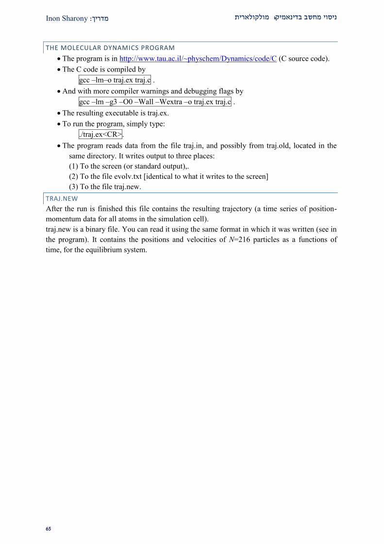
Inon Sharony: ךמדרי ניסוי מחשב בדינאמיקה מולקולארית
92
THE MOLECULAR DYNAMICS PROGRAM
The program is in http://www.tau.ac.il/~physchem/Dynamics/code/C (C source code).
The C code is compiled by
gcc –lm–o traj.ex traj.c .
And with more compiler warnings and debugging flags by
gcc –lm –g3 –O0 –Wall –Wextra –o traj.ex traj.c .
The resulting executable is traj.ex.
To run the program, simply type:
./traj.ex<CR>.
The program reads data from the file traj.in, and possibly from traj.old, located in the
same directory. It writes output to three places:
(1) To the screen (or standard output),.
(2) To the file evolv.txt [identical to what it writes to the screen]
(3) To the file traj.new.
TRAJ.NEW
After the run is finished this file contains the resulting trajectory (a time series of position-
momentum data for all atoms in the simulation cell).
traj.new is a binary file. You can read it using the same format in which it was written (see in
the program). It contains the positions and velocities of N=216 particles as a functions of
time, for the equilibrium system.

Inon Sharony: ךמדרי ניסוי מחשב בדינאמיקה מולקולארית
99
ח מכין"דו
Jones-Lenardמודל .2
.Lenard-Jones בפוטנציאל ביטוי לידי באים פיזיקאליים עקרונות אילו בקצרה ירוהסב .א
המופיעים פרמטריםמה אחד כל של הסביר הערכים וטווח הפיזיקאלית המשמעות מה .ב .Lenard-Jones בפוטנציאל
מה ?אפסמתי היא שווה ל ?חיוביתומתי שליליתהאנרגיה הפוטנציאלית מתי .ג ?ליותאהמשמעויות הפיזיק
אנרגיה כוללת האם תצפו ל, (חיובית)בהתחשב בכך שלמערכת יש גם אנרגיה קינטית .ד .נמקו? חיובית או שלילית
?כיצד יקבע הנרמול ?בהן תעשו שימוש בחלק הביצוע בשבוע זה מצומצמותהיחידות המהן .1 :תכניתהמבנה .2
.שניתנה של התכנית יחידהמה עושה כל ותאר .אכדי להפוך אותה לתכנית המתארת תנועה של מיטלהשאילו חלקים של התכנית אפשר .ב
?U(r), נתון חלקיק אחד בפוטנציאל חיצוני
כיצד והיכן הסבירו . המהירויותהתפלגות אתרו את אותו חלק של התכנית האחראי על .ג .בולצמנית של האנרגיההוא מוודא התפלגות
?לבכל אם ,םנעשי קירוביםאילו ?תשל המערכ תנאי השפהמטופלים כיצד והיכן .ד
בהן תומכת התכנית שתי הדרכיםמהן ?תנאי ההתחלהכיצד מטפלת התכנית בוהיכן .ה ?לקביעת מיקום האטומים ההתחלתי
?של המערכתתנועת מרכז המסה כיצד היא מטפלת ב .ו :קלט הפרמטרים של הסימולציה .1
?בשניותמהו זמן זה ? צעד הזמן ביחידות מצומצמותמהו גודל .א ?לקובץ הפלט( המסלול)המיקומים ומהירויות נכתביםכל כמה צעדי זמן .ב ?שניותמהו משך זה ב? (בצעדי זמן) אורך המסלולמהו .ג ?בסימולציה מספר החלקיקיםמה .ד ?בסימולציה הטמפרטורהמה .ה
אובתייכיצד .traj.new, (המסלול) קובץ הפלטמהו המבנה של קראו את קוד התכנית והסבירו .2 ?ם עליהםע חישוביאת הנתונים מקובץ הפלט לתוכנית שתבצ
(יחידותולא במספרים חסרי ותביחידות פיסיקליענו על הסעיפים הבאים ) גודל המערכת .9
? מהי האינטראקציה ביניהם? מערכת הסימולציהמרכיבים את כמה אטומי ארגון .א
?המערכת נפחמהו .ב
?תהמסה במערכ צפיפותמהי .ג
?התפלגות המהירויותלקבל מהתכנית עבור פונקצית מה תצפו .2

Inon Sharony: ךמדרי ניסוי מחשב בדינאמיקה מולקולארית
92
מפלט התכנית מקרוסקופייםחישוב גדלים .2
דוגמה לכל נוות, מרחביות פונקציות קורלציהזמניות ו פונקציות קורלציההסבירו מהן .א .אחת
."הניסויביצוע "בפרק מפונקציות קורלציהגדלים המחושבים האת בקצרה תארו .ב
ות דרך לחישוב פונקצית ההתפלגו שונות לחישוב מקדם הדיפוזיה שתי דרכים ותאר .ג .מפלט התכנית הזוגית הרדיאלית
? בתכנית מושפעת מתנאי השפהיכולה להיות ים אלוהאם תוצאת חישוב .ד ? אם בכלל, השפעה זושל תלות בזמן מה תהיה ה, וכןבמידה . מדוע וריהסב, ולאבמידה
(.של המערכת גדלים אופיינייםהבע במונחים של )
:אינטגרציה נומרית .ה
? הטרפזכלל מני והי, השמאלי סכום רימןמהו (2)
? האיברים משאר האיבר הראשון והאחרוןשונים מדוע רק בשיטת הטרפז (1)
.יותר לאינטגרלבטוב הקירוב האת איזה מהשלושה נותן וריהסב (2)
מספיק קרובות כך שהאינטגרנד מונוטוני השערוךבהנחה שנקודות (1) גרללאינט עליוןחסם מי משלושת סכומי רימן לעיל נותן , ביניהםשבמקטעים
(לא ניתן להניח שהפונקציה מונוטונית בין מקטעים שונים) ?מי תחתוןו
בהינתן מערך חד ממדי של משתנים עשרוניים המייצגים את ערכיה של (2) תרשים זרימה וגיהצ, dtבמרווחים קבועים השווים ל בתחום מסוים ופונקציה
.הטרפז כללבאמצעות , tלפי של הפונקציה אינטגרל הלחישוב קוד-או פסאודו
קוד-תרשים זרימה או פסאודו וגיהצ, bבסעיף ארתם ימשיטות החישוב שת תלכל אח .ו .מפלט התכניתלחישובם
שאלות בונוס
הקיימים ים אופיינייםבהתבסס על גדל, ליחידות אנרגיה מצומצמות אפשרות חלופיתהצע .2 ?מדוע? החלופי האם היא עדיפה על פני ההסבר. במערכת
.(DLS) פיזור אור דינאמינקצית ההתפלגות הזוגית הרדיאלית בניסוי פונדגמת הסבר כיצד .20
ניתן לקרב את , מקונפיגורציית האנרגיה הפוטנציאלית המינימאלית הסטים קטניםהראה שעבור .22-בתחתית בור פוטנציאל לנארדעקמומיות בטאו את ה .ונס כפוטנציאל הרמוני'ג-פוטנציאל לנרד
.ים של פונקצית הפוטנציאלבאמצעות הפרמטר עומקוונס ואת 'ג
עד כמה הן צריכות להיות נמוכות ? טמפרטורות נמוכותמדוע קירוב זה רלוונטי רק ב .א, חשבו מה צריכה להיות טמפרטורה זו עבור ארגון? ביחס לפרמטרים של הפוטנציאל
.של הניסוי זהבהינתן הפרמטרים בחלק
ית אוסילטור יחיד ין סימולצבהשוואה בין סימולציית מספר גדול של אטומי ארגון לבי .בחלקיקיות ואילו תכונות -אילו תכונות חד, (בשני המקרים הניחו תנאי שפה מחזוריים)
ערכו השוואה של היתרונות ? חלקיקיות ניתן לחשב בכל אחת מהסימולציות-רב .והחסרונות בכל גישה
!לזכות בבונוס פרטו כאן על מנת, (הכנה או ביצוע)אם גיליתם טעויות בפרק זה של התדריך .21

Inon Sharony: ךמדרי ניסוי מחשב בדינאמיקה מולקולארית
92
ביצוע הניסוי
תוכלו לבחור . באחת מכמה דרכים תלהיעשויכולה המולקולאריתהעבודה עם תכנית הדינאמיקה .2 .כל קומבינציה שנוחה לכם
:וסביבת העבודה בחירת מערכת ההפעלה .א
.LINUXהרצה ועיבוד התוצאות תחת , עריכה: 'אלטרנטיבה א (2)
ייצוא הפלט לעיבוד התוצאות , LINUXעריכה והרצה תחת : 'אלטרנטיבה ב (1)
.בסביבת עבודה אחרת
עריכת התכנית ועיבוד התוצאות , LINUXהרצה תחת : 'ג אלטרנטיבה (2)
.בסביבת עבודה אחרת
התאמת קוד המקור לעבודה מלאה בסביבת (: עתידית)' אלטרנטיבה ד (1)
.עבודה אחרת
:פורמט קבצי פלטבחירת .ב
.(מקור) קבצים בינאריים: 'אלטרנטיבה א (2)
לקובציניתן לשנות את קוד המקור כך שהפלט יודפס : 'רנטיבה באלט (1)
.טקסט
:תוצאותהסביבת עיבוד .ג
.נפרדת Cעיבוד התוצאות בתכנית : 'אלטרנטיבה א (2)
Cה תכנית תוך עיבוד התוצאות בשינוי קוד המקור ו: 'באלטרנטיבה (1) .המקורית
, הלדוגמ)עיבוד התוצאות במסד נתונים עם ממשק גרפי : 'גאלטרנטיבה (2)
OfficeLibre Calc)
, לדוגמה)עיבוד התוצאות בתכנה ללא ממשק גרפי : 'דאלטרנטיבה (1)
GNUPlot.)
שהתחיל מקונפיגורציה מסלול במצב שיווי המשקל עבור חישובים להשתמש בבפרק זה יש .1את התוצאות להציג ו (ארוך מספיק traj.oldכלומר שההתחלה שלו נלקחה מ )בשיווי משקל .יות ולא מצומצמותלאביחידות פיזיק
אנרגטיקה .2
לצד יחיד על גרף כסדרת נתונים מהמהירויות והציגו אותה האנרגיה הקינטיתחשבו את .אשל הכוללתהאנרגיה הפוטנציאלית והאנרגיה , האנרגיה הקינטית שנותנת התכנית
.במידה וישנה, התאמה-הסבירו כל אי. המערכת כפונקציה של הזמן
שגיאה הרגעית בדונו . כפונקציה של הזמן הכוללתאנרגיה ביחסי שימור הה-איהציגו את .בוהשוו לצבר המנותק מאמבט , באנרגיההיחסית באנרגיה ובשגיאה הממוצעת היחסית
(.האוסילטור ההרמוני מהפרק הקודם, לדוגמה)חום

Inon Sharony: ךמדרי ניסוי מחשב בדינאמיקה מולקולארית
92
מפרטורההתפלגות המהירויות וט .1 ?המהירויות שנמדדו תחוםמה .א
.v שלאטום הנבחר באופן אקראי יש מהירותהסיכוי :v(P( כתבו תכנית שתחשב את .בהשוו )לה ציפיתם לפונקציה התאיממבדקו אם היא , ציירו את הפונקציה המתקבלת
מתבטאים בכל אחת והסבירו אילו גדלים פיזיקאליים( בטבלה ודווחו דיוק ונכונות :מהתכונות הבאות
ערך חציוני וערך ממוצע, ערך מסתבר ביותר (2)
מומנט ראשון (1)
שנימומנט (2)
שונות (1)
סטיית תקן (2)
.על פני כל התחום P(v)האינטגרל מתחת לפונקציה (9) מתוך המהירויות הנתונות במסלולהאפקטיבית של המערכת הטמפרטורהחשבו את .ג
.והציגו אותה כנגד הזמן
של התפלגות המהירויות שהוגרלו לפונקציה אנליטית מנורמלת והציגו את התאמהבצעו .ד .משוואת הפונקציה
דם הדיפוזיה העצמית של ארגוןחישוב מק .2 !(צעדי זמן 1זכרו שהקואורדינאטות נכתבות לקובץ רק כל )
קורלציה עצמית של המהירות .א
כפונקציה הקורלציה פונקציתחשבו וציירו את (2)
שימו לב שהנוסחה פשוטה יותר כי .המיצוע הוא על גבי האטומים. tשל .
כיצד ?בזמנים קצרים או בזמנים ארוכים, הרלוונטין נמצא המידע היכ (1)ללא , יותר מדויקתכדי לקבל תוצאה *dtו א/ו tשל םאת ערכ יםמשנ םהיית
בשאלות .מחדש יצואת השינוי המוצע והר ובצע ?חישוביתההשקעה הגדלת ה .התמקדו בטווח הזמנים הרלוונטי ביותר לחישוב התשובות, שבהמשך
מה ? נקודות החיתוך עם ציר האבסיסהשל תהפיזיקאליות מה המשמע (2)שימו : רמז)? עבור הקורלציה העצמית של המהירות ערך שליליהמשמעות של
(יחידותלב ל
ב מקדם הדיפוזיה ושיחל( לפני ההתאמה)הנומרית השתמשו בתוצאה (1) .של ארגון בתנאים הנתונים העצמית
ממוצע ריבוע ההעתקה .ב
כפונקציה העתקהחשבו את ממוצע ריבוע ה (2)
. tשל
בסימולציה מה התנהגות ממוצע ריבוע ההעתקה בגבול של זמנים ארוכים (1) .הסבירו? שלכם
את ערכם יםמשנ םכיצד היית? הרלוונטינמצא המידע תחום של זמןבאיזה (2)? ללא הגדלת ההשקעה החישובית, יותר מדויקתכדי לקבל תוצאה *dtאו /ו tשל התמקדו בטווח , בשאלות שבהמשך .מחדש יצווי המוצע והראת השינ ובצע
.הזמנים הרלוונטי ביותר לחישוב התשובות
.מקדם הדיפוזיה העצמיתאת תוצאה זוקבלו גם מ (1)
, של הסימולציה לפרמטרים שנבדקו בעבר בניסוי קפילרי ובסימולציה שנו את הפרמטרים .ג (.דיוק ונכונות דווחו)הריצו מחדש והשוו את תוצאותיכם אליהם בטבלה

Inon Sharony: ךמדרי ניסוי מחשב בדינאמיקה מולקולארית
20
ענו על שאלת ההכנה הבאה מהחלק הראשון בניסוי והשוו לתוצאותיכם ולתוצאות .ד .בספרות
דיפוזיה של חלקיק בתוך נוזל של )העריכו את מקדם הדיפוזיה העצמית (2)המהלך החופשי הממוצע ומשך המהלך החופשי באמצעות אורך ( אותם חלקיקים
שלו רדיוס והמסת החלקיק , הנוזלבטאו התוצאה באמצעות צפיפות . הממוצע .והטמפרטורה( חתך פעולה קלסי)
ק "גרם לסמ 2.221בצפיפות מקדם הדיפוזיה העצמית של ארגון העריכו את (1)השוו לתוצאה ניסיונית מהספרות עבור צפיפות קלווין ו 21.1וטמפרטורה
.נגסטרםוא 2.22, השתמשו ברדיוס ואן דר וולס של ארגון .וטמפרטורה דומות
.תהניסיוניודיוק בתוצאות החישובים ביחס לתוצאות -ציעו סיבות לאיה .ה
הרדיאלית הזוגית התפלגותהפונקצית .9
הסתברות מותנית של מיקומי פונקציתהינה ,g(r), פונקצית ההתפלגות הזוגית הרדיאלית .אשל מרחקי כל מנורמלת היסטוגרמה באמצעותנומרית אותה לחשב ניתן . האטומים
הזוגית ההתפלגותחשבו את פונקצית . ביחס למיקום האחד, חד מהםהאטומים מלבד א .ונתחו את צורתה r כפונקציה של, הרדיאלית
גם את לבדוקיש עבור כל אטום ,כלומר .יש להתחשב בתנאי השפהשימו לב ש :הדרכהבדקו זאת .מבין שני אלה אל אטום הייחוסלכלול בחישוב רק את הקרוב אז דמותו ו
.לחוד( x,y,z) עבור כל ממד
?(r/σגדולים של קטנים וערכים , כלומר) גבולות מרחקים קצרים וגדוליםבמתקבל מה .ב
של הסימולציה לאלו שנבדקו בעבר בניסוי פיזור קרני רנטגן מארגון שנו את הפרמטרים .ג (. דווחו דיוק ונכונות)השוו את תוצאותיכם אליהם בטבלה נוזלי ו
.החישובים ביחס לתוצאות הניסיוניות דיוק בתוצאות-הציעו סיבות לאי .ד
בונוס יתרגיל
(.D)ממקדם הדיפוזיה ( )בנוזל מקדם החיכוךאת וחשב, , בהינתן קשר איינשטיין .2
.של הניסוי' בחלק ב שיישמתםאחת השיטות ב, של פתרון משוואות התנועה סימטריה בזמן בדקו .2
:הדחיסה וגזירמאמצי התגובה ל – לחץ וצמיגות .2
הוא התגובה של ( האיזוטרופי)הלחץ :חשבו את הלחץ בנוזל מתוצאות הסימולציה .אוהאטומים מגיבים ונעים , כוח מופעל בכיוון נתון) מסויםהמערכת למאמץ דחיסה בכיוון
(.באותו כיוון :(הויריאל שנגזרתו בזמן היא)ממומנט האינרציה לחשב את הלחץ ניתן
מאמץ לא תגובה של הנוזל יההצמיגות :ות הסימולציהחשבו את צמיגות הנוזל מתוצא .ב
.(והמופעל על הנוזל בכיוון מסוים גורם לחלקיקים לנוע בכיוון ניצב ל חכו)גזירה :הלחץ האנאיזוטרופיניתן לחשב את צמיגות הנוזל מהקורלציה בין
ii. i.
iv. iii.
של אנאיזוטרופיותד לגבי המה תוכל להגי, בהינתן מערכת בה .ג ?של המערכת המבנה המרחבי, לדעתך, מה יהיה? המערכת

Inon Sharony: ךמדרי ניסוי מחשב בדינאמיקה מולקולארית
22
:נבולוציהרלציה וקוקו, קורלטור .20
,fiקורלטור של הפונקציה -אם נגדיר את האוטו
מכיוון , auto-covariance, בעצם השונות המשותפת העצמית) קורלציה-נוכל לבטא את האוטו
,(fלפי השונות של נרמולשאין
1
10 0,
i i
N
Ni
t t t G tN
ff ff f ff f
,(auto- cross-variance)העצמית הצולבתהשונות
*
0 0
0 0
*
1
1lim lim ,
f f
i if f
t t t tN
t t t tit t
N
C t t d G t dN
ff f ff f
,(קורלציה הצולבת-ממשית שווה לתמונת הראי של האוטו fשבמקרה שבו ) והקונבולוציה
0 0
0 01
1lim lim ,
f f
i if f
t t t tN
t t t tit t
N
g t t d G t d C tN
ff f f fff f
ולאחר מכן לעבוד רק עם , מן אפסבז fבכדי לחשב את הקורלציה יש לשמור את ערך הפונקציה בכדי לחשב את , לעומת זאת. 'גכפי שעשינו זה עתה בפרק , הנוכחי tערך הפונקציה בזמן
. 'אכפי שעשינו בפרק , t, בכל הזמנים fכל ערכי הפונקציה יש לשמור את , הקונבולוציהדרישות הזיכרון בהיבט, בכל מקרה הדבר מכביד על המערכת, ניתן לעשות זאת במערך או בקובץ
.בהתאמה, הפנימי או הזיכרון הקשיח וזמן החישובאך הפעם , חשבו פעם נוספת את מקדם הדיפוזיה מהקורלציה העצמית במהירויות .א
.דווחו דיוק ונכונות .החלפת חישוב הקורלציה בחישוב הקונבולוציהב. הצולבתלשונות אין הבדל בין הקונבולוציה סטציונאריראיתם שעבור תהליך ' בפרק א .ב
?האם קיבלתם שכך הדבר גם במקרה הנדון כעתקורלציה של המהירויות או -האוטו פונקציתעבור אין ביטוי אנליטי פשוט: הערה .ג
אפילו לא עבור מודל פשוט כמו מערכת של כדורים , ההתפלגות הזוגית הרדיאלית. ויים סגוריםאך הם אינם ביט, פשוטים בצורתם םאינטגראלייישנם ביטויים . קשיחים
' פרופעבודה נעשתה בתחום על ידי . אין ביטוי פשוט עבור תוצאת האינטגרל, כלומר .ביקסון

Inon Sharony: ךמדרי ניסוי מחשב בדינאמיקה מולקולארית
21
.המסלולאנימציה של על מנת לאפשר , XYZ.*בפורמט הדפיסו את כל הקונפיגורציות כקובץ .22ן שהיא ויזואלית מכיוו תזוהי אחת הבדיקות הנפוצות ביותר בדינאמיקה מולקולארי
, Jmol ןכגו (חינמיות) ניתן לצפות באמצעות תוכנות XYZפורמט אנימציה בב .איטיביתאינטוו
Avogadro , אוVMD. ךכ ,הלדוגמ ,ההקובץ ירא: Line
1 216
2 This is a comment line (can be blank): Argon cluster (216 atoms big) frame 1
3 A 0.000000 0.000000 0.000000
4 A 0.000000 0.000000 1.089000
.
.
.
218 A -0.513360 -0.889165 -0.363000
219 A -0.513360 -0.889165 -0.363000
220 216
221 This is a comment line (can be blank): Argon cluster (216 atoms big) frame i
222 A x(atom 1, frame i) y(atom 1,frame i) z(atom 1, frame i)
223 A x(atom 2, frame i) y(atom 2, frame i) z(atom 2,frame i)
…
438 A x(atom N-1, frame i) y(atom N-1, frame i) z(atom N-1, frame i)
439 A x(atom N, frame i) y(atom N, frame i) z(atom N, frame i)
…
348582 216
348583 This is a comment line (can be blank): Argon cluster (216 atoms big) frame 1600
348584 A 0.010000 0.000000 0.000000
348584 A -0.010000 0.000000 1.089000
…
348796 A -0.523360 -0.889165 -0.363000
348797 A -0.503360 0.889165 -0.363000
מכיוון (. היסוד, לדוגמה)האטום " סוג"בעמודה הראשונה בכל שורה מייצגת את Aהאות .איש לסמן , לא תומכת ביסודות האצילים כאטומים שיכולים להשתתף במולקולה Jmolש
.המייצגת אטום אחר Aאת האטומים באות
בכל עבור אותו אטום ו) Aסמנו אותו באות השונה מ , כדי לעקוב אחרי אחד האטומים .בולכן ייצבע )האטום יזוהה כאטום של יסוד אחר , כך(. XYZ.*הקונפיגורציות בקובץ ה
הריצו את האנימציה פעם נוספת וצפו במהלך האקראי שמבצע האטום (. בצבע אחר .שבחרתם
צרפו , במידה ועשיתם זאת(. gif.*לדוגמה בפורמט )תוכלו גם לייצא את האנימציה כקובץ .ג .ח המסכם"אותו לדו