Moldflow Technology

Recent Developments &

Data Requirements

NPL March 12 2008

Who we are

Global Operations

Corporate HQResearch & DevelopmentDirect Sales & SupportManufacturing Center

Distributors & Mfg’s Reps

Moldflow Products – Core Modules

� Injection moulding:

– MPI/Flow

– MPI/Cool

– MPI/Warp

Other Simulation Applications

� Design of Experiments

� Mould core deflection

� 2-shot, Co-injection

� Gas assist

� Injection-compression

� Insert overmoulding

� Micromoulding

� Rubbers & Thermosets, incl warpage

� Liquid Crystal Polymers

� MuCell

� Birefringence

� Interface to FEA (structural loading)

Fill Pattern Verification

Moldflow prediction for flow pattern near end of fill

Short shots to show actual flow pattern near end of fill

Short shot digital photos to match above

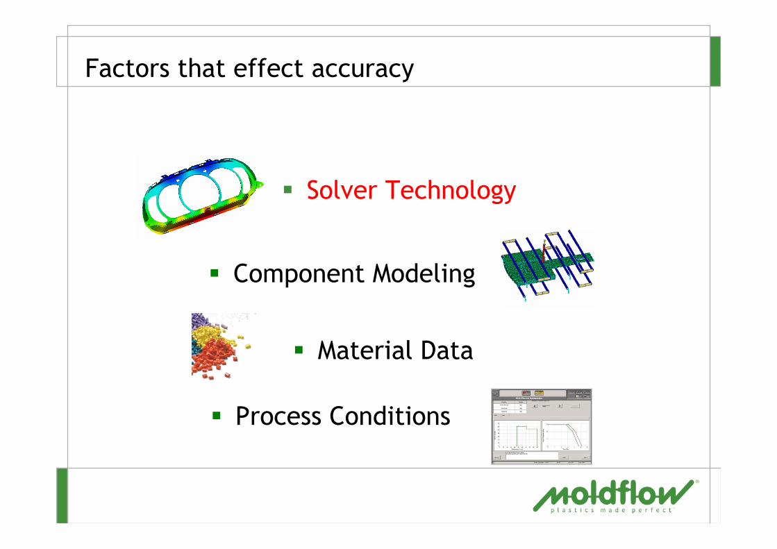
Factors that effect accuracy

� Solver Technology

� Component Modeling

� Material Data

� Process Conditions

Solver Improvements

� Gravity effects

– For low viscosity materials

� Polymer jetting flow

– Causes flow marks on surface

– Polymer jet buckles, touches mould and

cools

Beginning

Compressive Heating Added

� Compressive heating added to energy

equation for fluid flow

� Melt temperature will increase as the

material gets compressed

MPI 6.0

MPI 6.1

� Generally pressures will be

4% to 5% lower than before

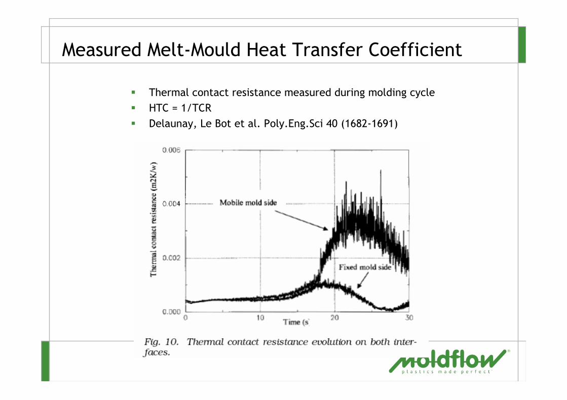
Measured Melt-Mould Heat Transfer Coefficient

� Thermal contact resistance measured during molding cycle

� HTC = 1/TCR

� Delaunay, Le Bot et al. Poly.Eng.Sci 40 (1682-1691)

3-Stage Heat Transfer Coefficient (HTC)

� Flow Solvers now use 3-stage HTC

� Defaults

– 5000 W/m2 Filling

– 2500 W/m2 Packing

– 1250 W/m2 Detached (pressure = 0)

Factors that effect accuracy

� Solver Technology

� Component Modeling

� Material Data

� Process Conditions

� Mechanical Properties

� Twin BoreCapillary Rheometer

� Shrinkage for non-fibre materials

� pvT for Thermosets

Ithaca,NY, US

� Visco-elastic

� ThermosetChemo-Rheometry

� Shrinkage for fibrematerials

� No flow temperaturefor LCP’s

Melbourne,Australia

Test Resources

� Injection Molding Rheometry

� Shrinkage testing

� Pressure Volume Temperature

� Thermal conductivity

� Differential Scanning Calorimetry

� Solid Density

� Shrinkage Measurements

� Moisture Measurement

� Material Conditioners

� Environmental Control

Melbourne + Ithaca, NY

International Standards

Injection Molding Rheology:

• ASTM D5422 Standard Test Method for Measurement of Thermoplastic Materials by Screw-Extrusion Capillary Rheometer

• ASTM D3835 Standard Test Method for Determination of Properties of Polymeric Materials by Means of a Capillary Rheometer

• ISO-11443 Plastics - Determination of the fluidity of plastics using capillary and slit-die rheometers

Thermal Conductivity:

• ASTM D5930, Standard Test Method for Thermal Conductivity of Plastics by Means of a Transient Line-Source Technique

Differential Scanning Calorimetry:

• ASTM E1269 Determination of Specific Heat Capacity by Differential Scanning Calorimeter

• ASTM D3417 Enthalpies of Fusion and Crystallization of Polymers by Differential Scanning Calorimeter

• ASTM D3418 Transition Temperatures of Polymers by Differential Scanning Calorimetry

Mechanical Properties:

• ASTM D-638 Tensile Properties of Plastics

• ASTM E-132 Poisson’s Ratio at Room Temperature

Coefficient of Thermal Expansion:

• ASTM D-696 Coefficient of Linear Thermal Expansion of Plastics

American Association for Laboratory Accreditation

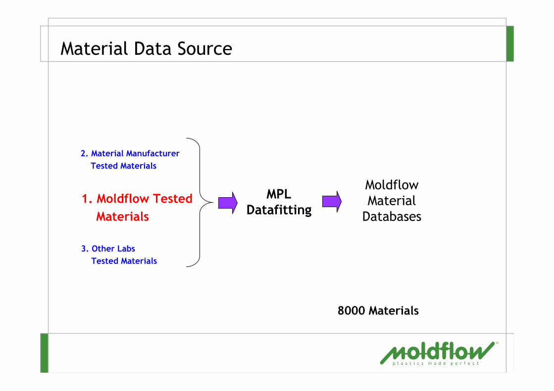
Material Data Source

Moldflow

Material

Databases

MPLDatafitting

1. Moldflow Tested

Materials

2. Material Manufacturer

Tested Materials

3. Other Labs

Tested Materials

8000 Materials

Capillary rheometers

� Rosand RH-7

– Classic method

(offline)

– Reservoir/Plunger

– Long residence times

� IMR

– Moulding machine

method (online)

– Charge/Shutoff Screw

– Short residence times

– Suitable for high

performance

materials

Test section

Modified Cross-WLF model

� Cross model captures the shear rate sensitivity of most material

families

� WLF equation captures exponential-hyperbolic temperature

sensitivity depending on the magnitude of T-T*

RamOil catch pan

SpacerThermocouple block

Water jacket

Heater

Control thermocouple

Bellows piezometer

Micrometer

Drainvalve

Burst-disc

Electric pump

High-pressurehand pump

Heat sink

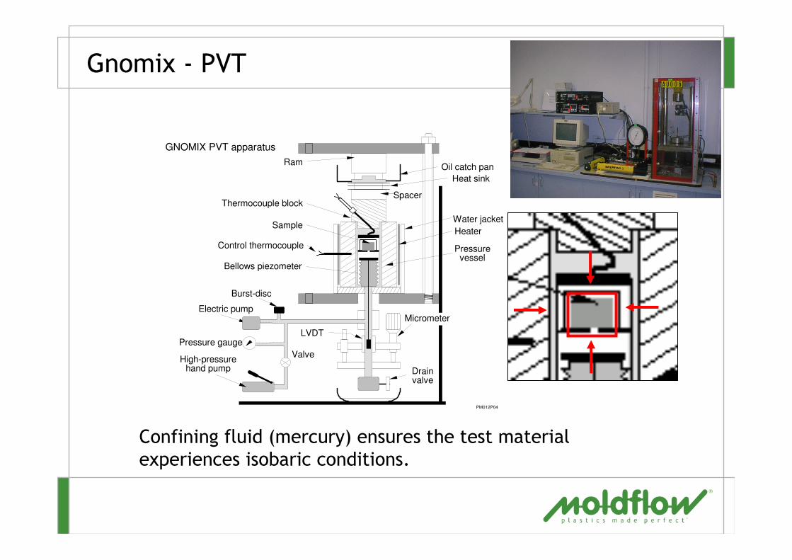
GNOMIX PVT apparatus

Valve

Pressure gauge

Sample

LVDT

Pressurevessel

PM012P04

Gnomix - PVT

Confining fluid (mercury) ensures the test material

experiences isobaric conditions.

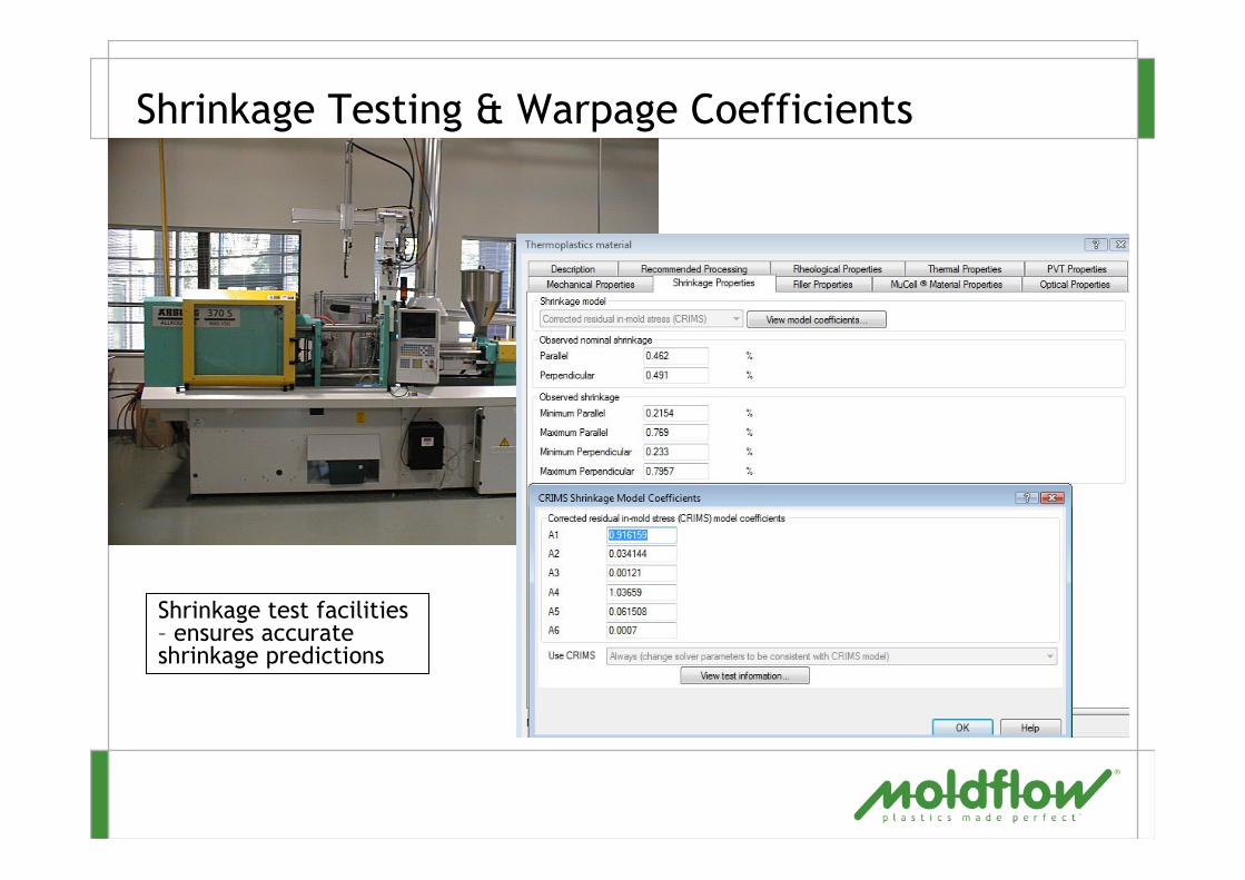
Shrinkage Testing & Warpage Coefficients

Shrinkage test facilities – ensures accurate shrinkage predictions

Thermal Conductivity K-System II

Thermal conductivity vs Temperature

0

0.05

0.1

0.15

0.2

0.25

0.3

0.35

0.4

0 50 100 150 200 250 300

Temperature (°C)

Th

erm

al c

on

du

cti

vit

y k

(W

/m-C

)

Multi-point thermal conductivity data

Thermal conductivity vs Temperature

0

0.05

0.1

0.15

0.2

0.25

0.3

0.35

0.4

0 50 100 150 200 250 300

Temperature (°C)

Th

erm

al c

on

du

cti

vit

y k

(W

/m-C

)

Single Point Thermal Data

Multi Point Thermal Data

Cooling Uses Multi-Point Thermal Data

� Now the cooling solver uses multi-point

thermal data for heat flux calculations

in the part

� Results typically will have

only a subtle change

Single point Multi point

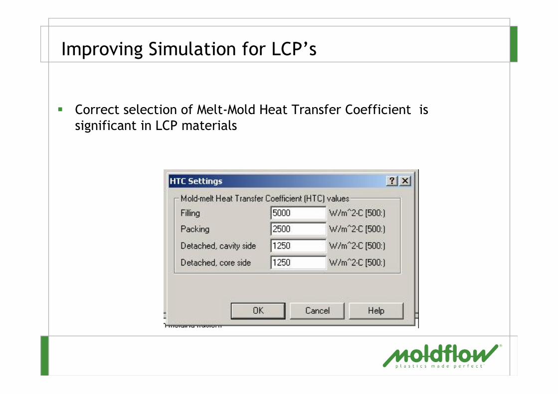
Improving Simulation for LCP’s

� Correct selection of Melt-Mold Heat Transfer Coefficient is

significant in LCP materials

LCP – Unusual behaviour at low rates

� LCP – “three region” flowGuo, T., Harrison, G.M., and Ogale, A.A., "Rheology and microstructure of

thermotropic liquid crystalline polyesters," Antec (2001).

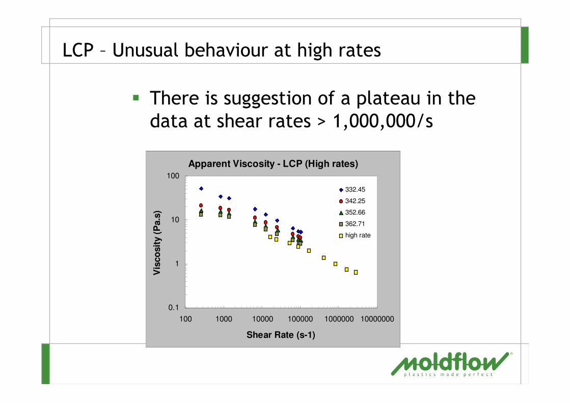
LCP – Unusual behaviour at high rates

� There is suggestion of a plateau in the

data at shear rates > 1,000,000/s

Apparent Viscosity - LCP (High rates)

0.1

1

10

100

100 1000 10000 100000 1000000 10000000

Shear Rate (s-1)

Vis

co

sit

y (

Pa.s

)

332.45

342.25

352.66

362.71

high rate

LCP – Complex temperature dependence

� Y.Fan, S.Dai and R.I. Tanner; Korea Australia Rheology Journal 15 (2003) 109

The Matrix Model

� Can capture unusual transitions that the

Cross model cannot

LCP - thermal conductivity and depth

� The variation in conductivity in the skin and core layers

can be measured by milling to different depths

k=0.20W/mK

k=0.23W/mK

k=0.40W/mK

skin core

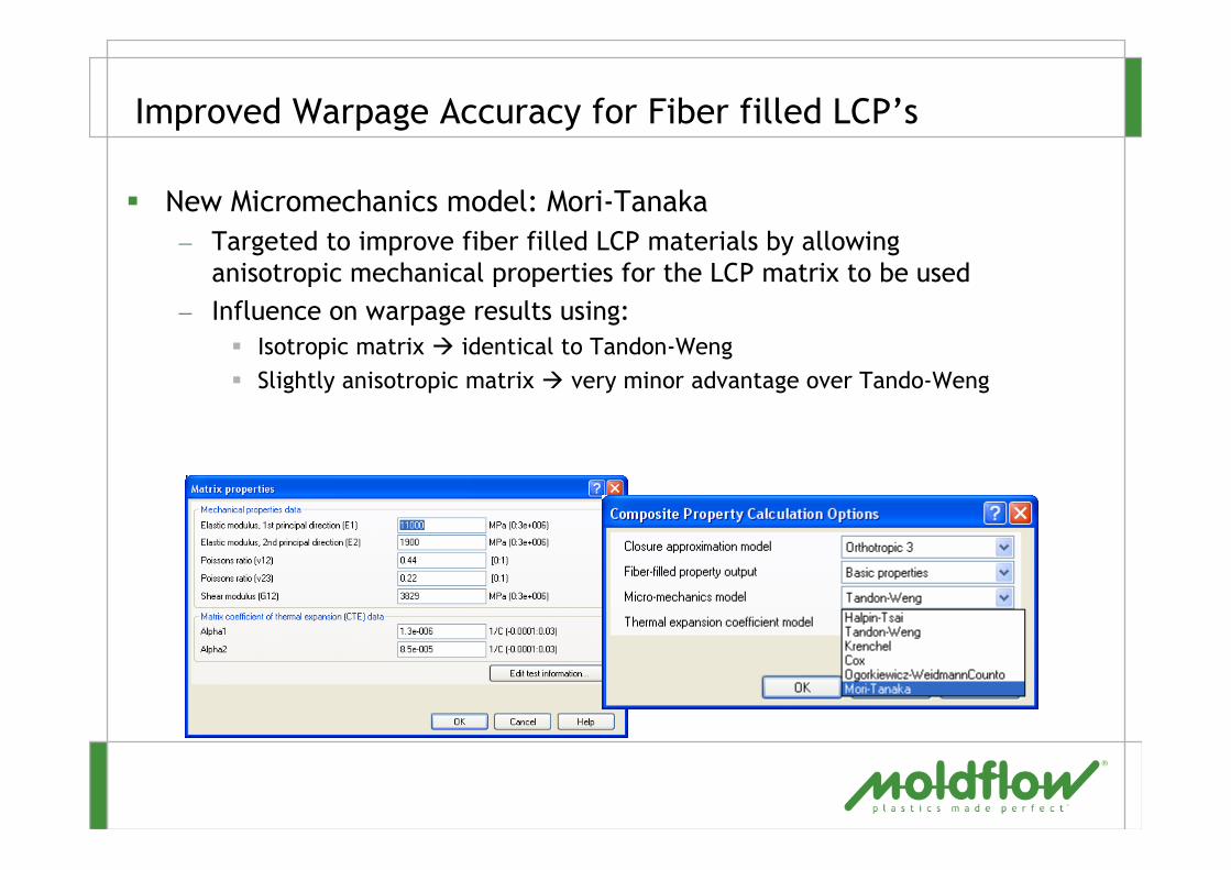
Improved Warpage Accuracy for Fiber filled LCP’s

� New Micromechanics model: Mori-Tanaka

– Targeted to improve fiber filled LCP materials by allowing

anisotropic mechanical properties for the LCP matrix to be used

– Influence on warpage results using:

� Isotropic matrix � identical to Tandon-Weng

� Slightly anisotropic matrix � very minor advantage over Tando-Weng

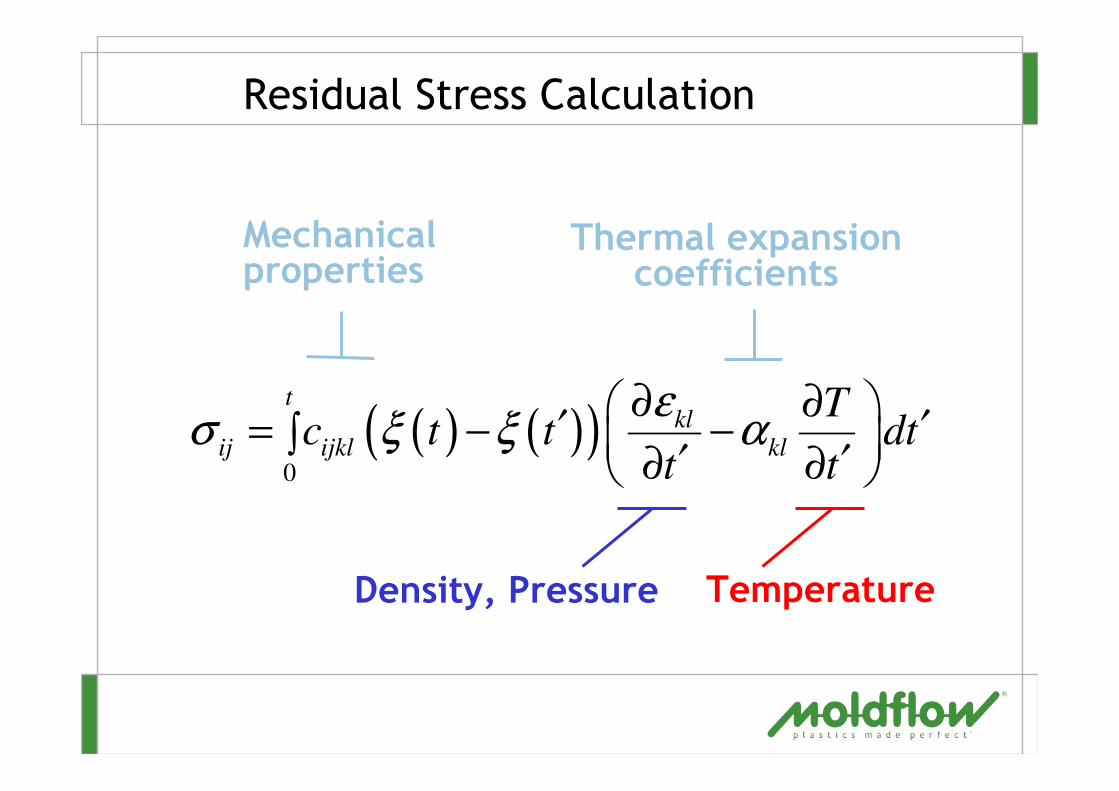
Residual Stress Calculation

( ) ( )( )0

tkl

ij ijkl kl

Tc t t dt

t t

εσ ξ ξ α

∂ ∂ ′ ′= − −∫ ′ ′∂ ∂

Mechanical Properties Total Strain

σ = E ε×

Residual Stress Calculation

( ) ( )( )0

tkl

ij ijkl kl

Tc t t dt

t t

εσ ξ ξ α

∂ ∂ ′ ′= − −∫ ′ ′∂ ∂

Mechanical properties

Thermal expansion coefficients

Density, Pressure Temperature

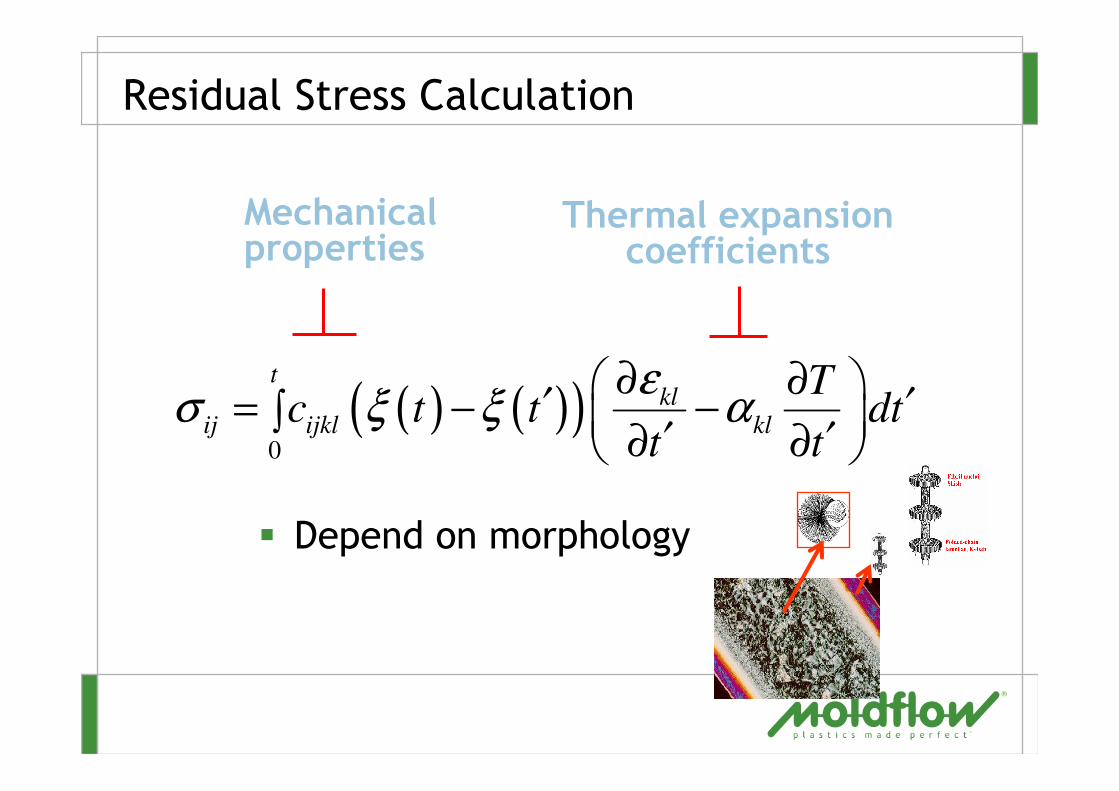
Residual Stress Calculation

� Depend on morphology

( ) ( )( )0

tkl

ij ijkl kl

Tc t t dt

t t

εσ ξ ξ α

∂ ∂ ′ ′= − −∫ ′ ′∂ ∂

Mechanical properties

Thermal expansion coefficients

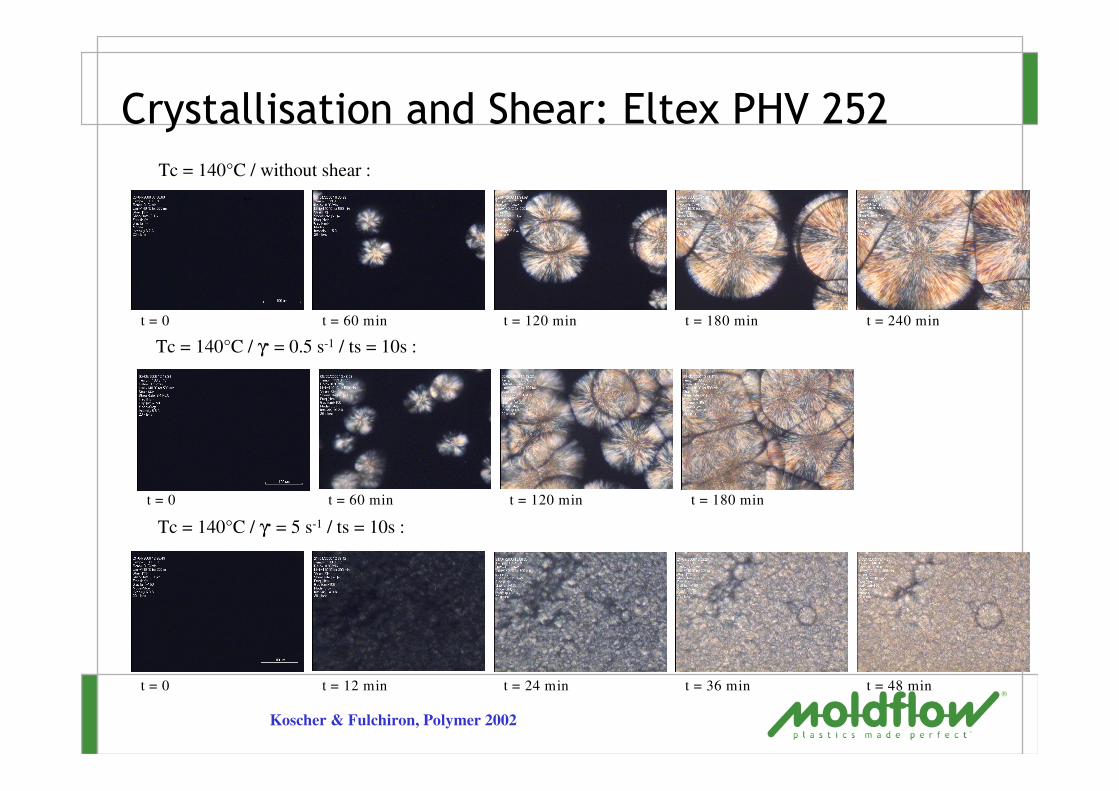
Crystallisation and Shear: Eltex PHV 252

Tc = 140°C / γ. = 0.5 s-1 / ts = 10s :

Tc = 140°C / γ. = 5 s-1 / ts = 10s :

Tc = 140°C / without shear :

t = 0 t = 60 min t = 120 min t = 180 min t = 240 min

t = 180 mint = 120 mint = 60 mint = 0

t = 0 t = 12 min t = 24 min t = 36 min t = 48 min

Koscher & Fulchiron, Polymer 2002

Crystallisation

� Shear– Affects nucleation

– Decreases crystallisation timeEder, Janeschitz Kriegl, Lidauer, Prog. Polymer Sci. 1990

� High shear for short time more effective than low shear for longer time

Vleeshouwers and Meijer - Rheol. Acta. 1996

� Shearing for longer periods affects morphology– Crystallisation time unchanged

– Formation of row nucleiKumaraswamy et. al. - Macromolecules 1999.

Acierno et. al. - Rheol. Acta. 2003.

Koscher and Fulchiron, Polymer, 2003.

Effect of FIC on Viscosity

shear rate (s-1

)

0.1

1

10

100

10 100 1000 10000

Time (s)

Sh

ea

r v

isc

osit

y (

η/η

η/η

η/η

η/η

00 00) ) ) ) 0.01

10

100

T = 140oC

For rough particles A ~0.44 Tanner - JNNFM 2002

Crystallisation & Conductivity

( )1 1 11 a sα α− − −= − +k k k

Slab model

a: amorphous phase

s: solid (semi-crystalline) phase

α: relative crystallinity

0.150.150.150.150.20.20.20.2

0.250.250.250.250.30.30.30.3

0000 50505050 100100100100 150150150150 200200200200 250250250250 300300300300Temperature (DegC)Temperature (DegC)Temperature (DegC)Temperature (DegC)Thermal Conductivity (W/m-C)Thermal Conductivity (W/m-C)Thermal Conductivity (W/m-C)Thermal Conductivity (W/m-C)

Cooling rate increases

(Experimental data

P. Geraldine, PhD thesis, University of Nantes, 2002)

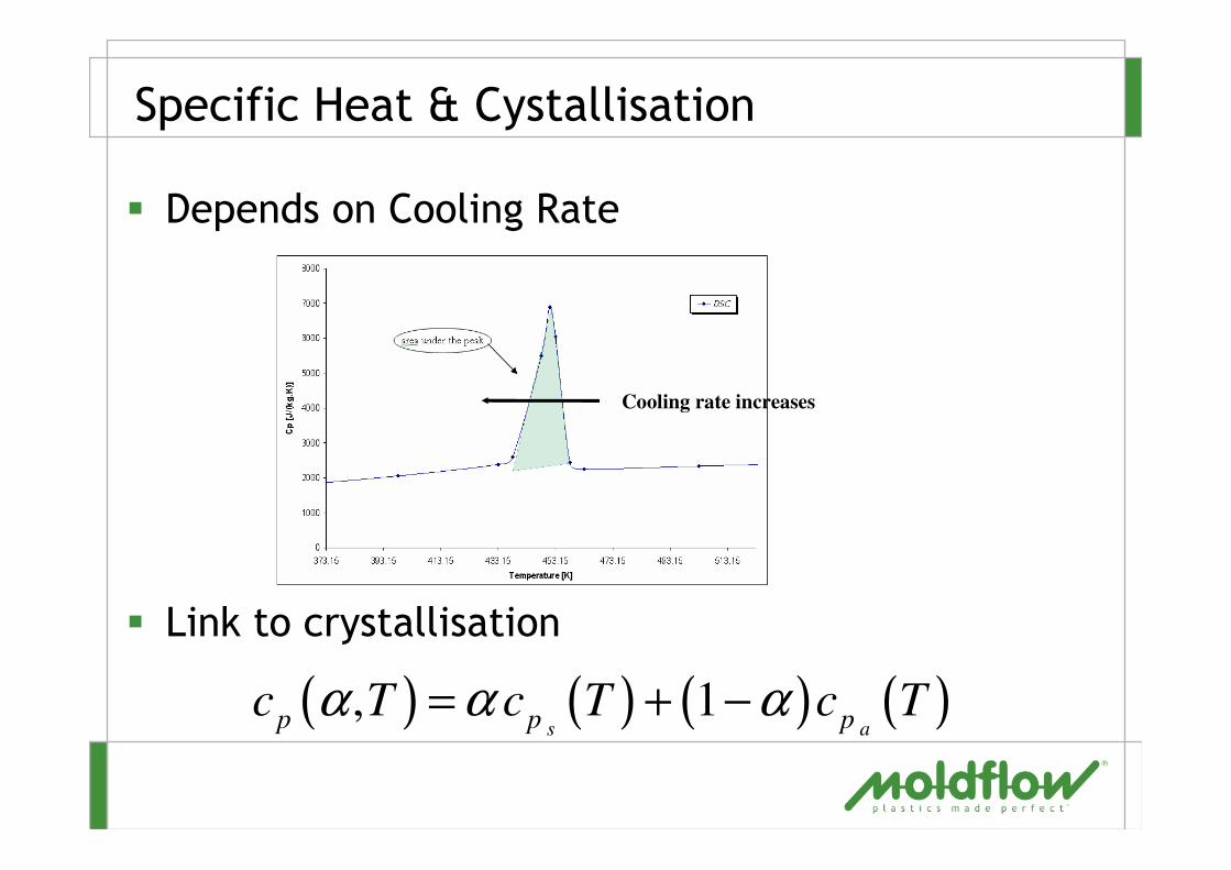
Specific Heat & Cystallisation

� Depends on Cooling Rate

� Link to crystallisation

Cooling rate increases

( ) ( ) ( ) ( ), 1s ap p p

c T c T c Tα α α= + −

Density & Crystallisation

� PVT measured under “static” conditions

� Modify with crystallisation

– Flow induced

– Temperature and rate of temperature change

Crystallisation Model

� Kolmorgoroff

� Accounts for affect of

– Temperature

– Rate of temperature change

– Flow induced crystallisation

( ) ( ) dsduuGsNC

mt

s

t

0mf

∫∫=α &

( )fexp1 αα −−=

Pressure Predictions

� PP (thickness=3.0mm)

New Results

Young’s Modulus (1mm part)

0

1000

2000

3000

-0.60 -0.40 -0.20 0.00 0.20 0.40 0.60

Depth (mm)

Yo

un

g M

od

ulu

s (

MP

a)

E // - 1 mm En - 1 mm

Experiments Prediction

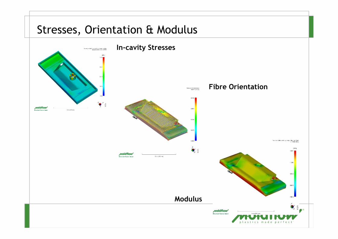
Stresses, Orientation & Modulus

Fibre Orientation

Modulus

In-cavity Stresses

Structural Analysis (FEA)

� Interface to:

– Abaqus

– Ansys

– Patran

– Nastran

– LS-Dyna Exclusive structural

analysis for optimising

the structural integrity

of plastic injection

moulded parts.

Information Exported from Moldflow to FEA

– Unfilled Materials� Elastic modulus, Shear modulus & Poisson’s ratio

from Material database

� Coefficient of thermal expansion (CTE) from

Material database

� Layer-wise (20 layers through the thickness of

each element) Residual stresses

– Fiber-filled Materials� Layer-wise Elastic modulus, Shear modulus &

Poisson’s ratio

� Layer-wise CTE

� Layer-wise Residual stresses

� Layer-wise Fiber orientation angle

Example

Case Nokia 6230Primary stiffening cover, essentialfor the entire phone stiffness

Stress Comparison

–Traditional stress analysis:

σvonmises=14.4 MPa

–Fully integrated analysis:

σvonmises=35.9 MPa

–Fully integrated analysis:

σvonmises=80.1 MPa

–Traditional stress analysis:

σvonmises=17.2 MPa

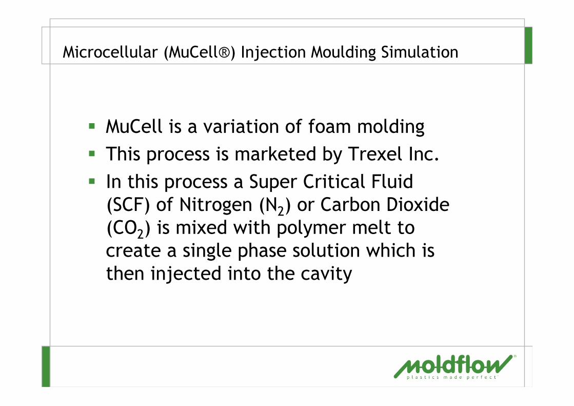
Microcellular (MuCell®) Injection Moulding Simulation

� MuCell is a variation of foam molding

� This process is marketed by Trexel Inc.

� In this process a Super Critical Fluid

(SCF) of Nitrogen (N2) or Carbon Dioxide

(CO2) is mixed with polymer melt to

create a single phase solution which is

then injected into the cavity

1. Creation of a single

phase solution

2. Homogeneous

Nucleation

3. Cell Growth

4. Part Formation

The MuCell ProcessThe MuCell Process

Image courtesy of Trexel Inc.

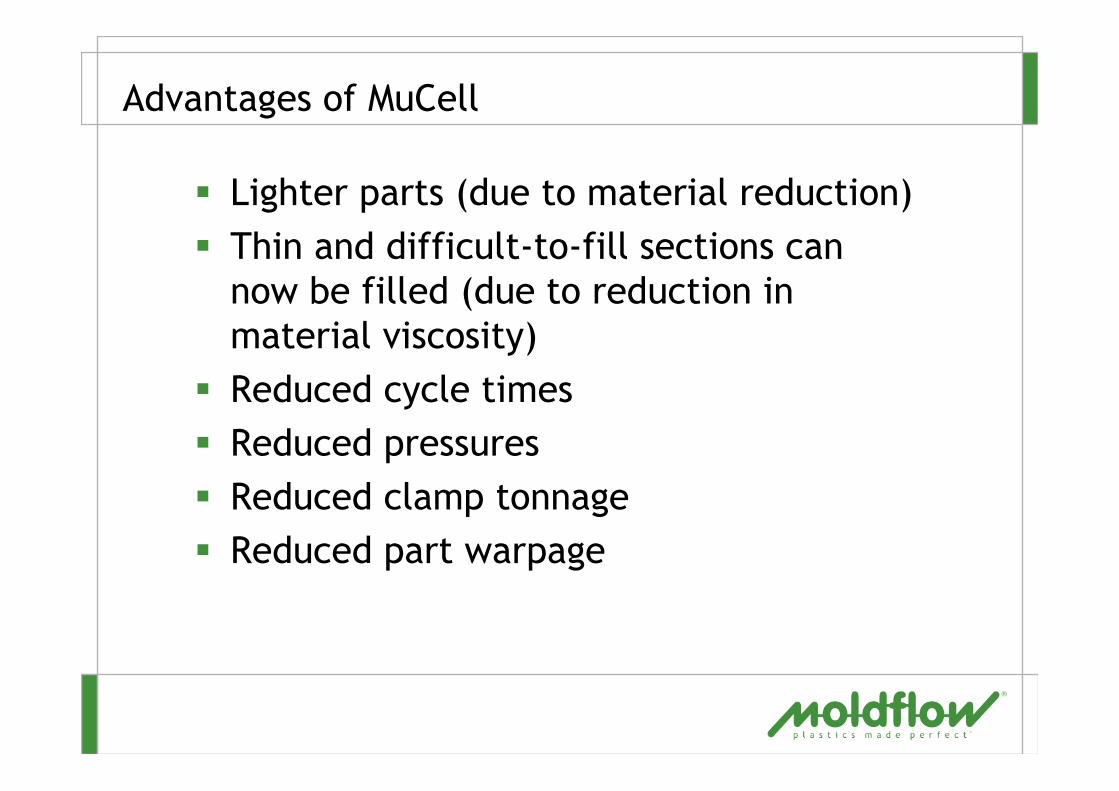
Advantages of MuCell

� Lighter parts (due to material reduction)

� Thin and difficult-to-fill sections can

now be filled (due to reduction in

material viscosity)

� Reduced cycle times

� Reduced pressures

� Reduced clamp tonnage

� Reduced part warpage

MuCell Gas Properties

MuCell User Inputs

Simulation Results

Bubble Radius at the end of cycle

Simulation Results

Bubble Radius as a function of time

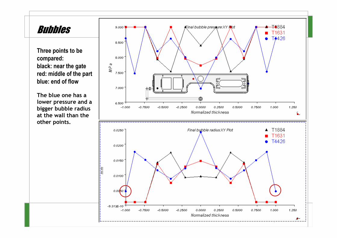
Bubbles

Three points to be

compared:

black: near the gate

red: middle of the part

blue: end of flow

The blue one has a lower pressure and a bigger bubble radius at the wall than the other points.

Simulation Results

Predicted Shape & Magnitude of part deflection

Clamp

force

Lower clamp force

with MuCell

MuCell Validation

Short shot comparison for gas concentration of 0.5% (by weight) and shot size of 70%

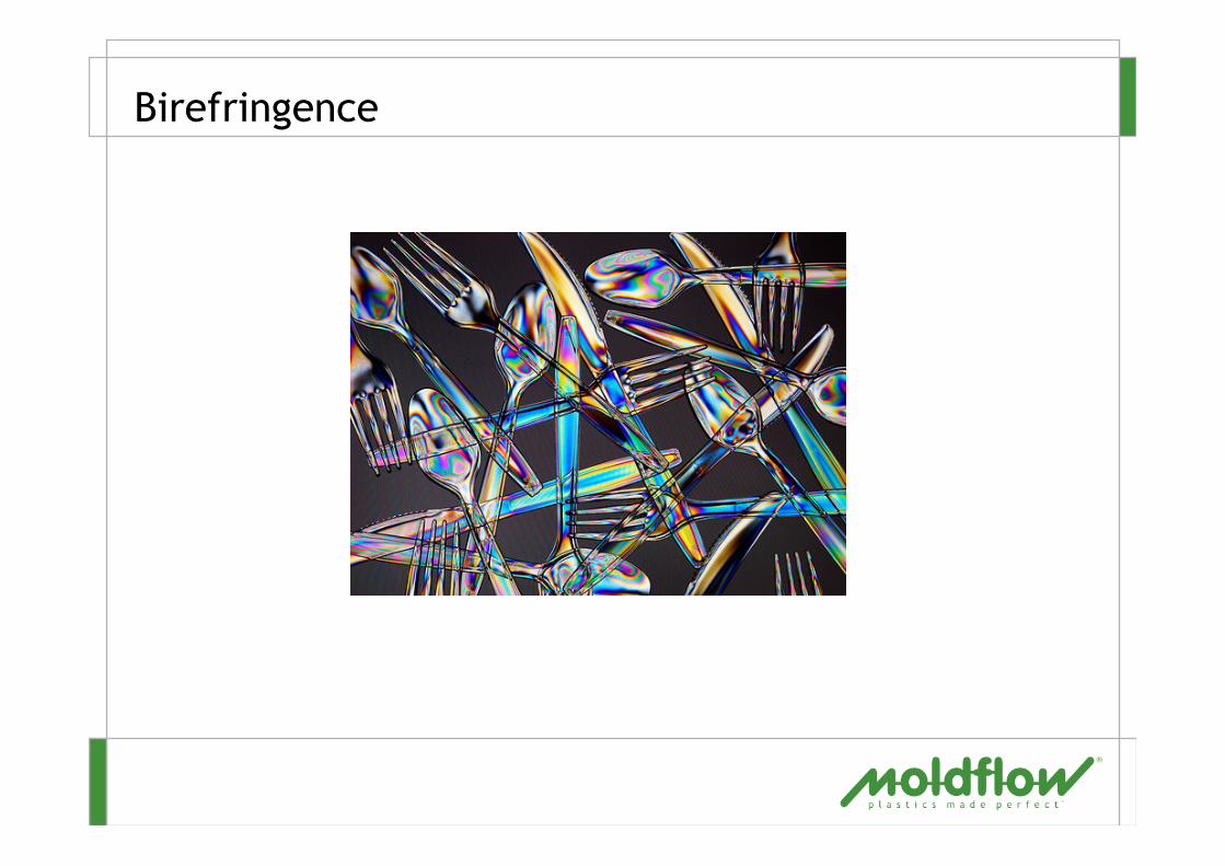
Birefringence

What is Birefringence?

� Definition: Birefringence is the change in

the refractive index of polarised light

passing through an object

� Birefringence may lead to crucial part

defects

– Blurred images

– Double images

– Poor optical performance

Birefringence: Polymers

� Birefringence can be caused by

stresses in polymer

– Flow induced stresses

– Post warpage induced stresses

� Elastic deformation caused by

residual stresses

� Viscoelastic deformation caused by

flow orientation of polymer

� Will not be uniform in all regions of

the part or through the thickness

� Need viscoelastic material data to

predict change in optical properties

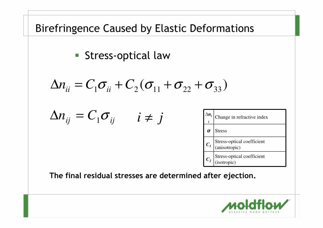
Birefringence Caused by Elastic Deformations

� Stress-optical law

)( 33221121 σσσσ +++=∆ CCn iiii

ijij Cn σ1=∆ ji ≠

The final residual stresses are determined after ejection.

∆ni

i

Change in refractive index

σ Stress

C1

Stress-optical coefficient

(anisotropic)

C2

Stress-optical coefficient

(isotropic)

Generalized Voigt-Kelvin Model

� Complex viscoelastic behaviour can be

described by elements with different

properties, coupled in series

∑

∑

=

λ−

=

λ−

λ−

−=τ

γ=

−τ=γ

−τ=γ

n

1i

/t

i

o

n

1i

/t

io

/t

ioi

)e1(J)t(

)t(J

)e1(J)t(

)e1(J)t(

i

i

i

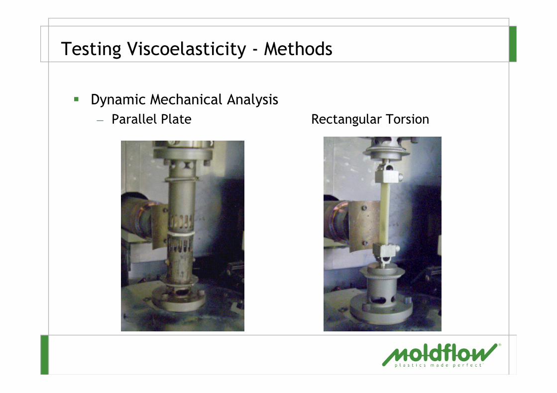
Testing Viscoelasticity - Methods

� Dynamic Mechanical Analysis

– Parallel Plate Rectangular Torsion

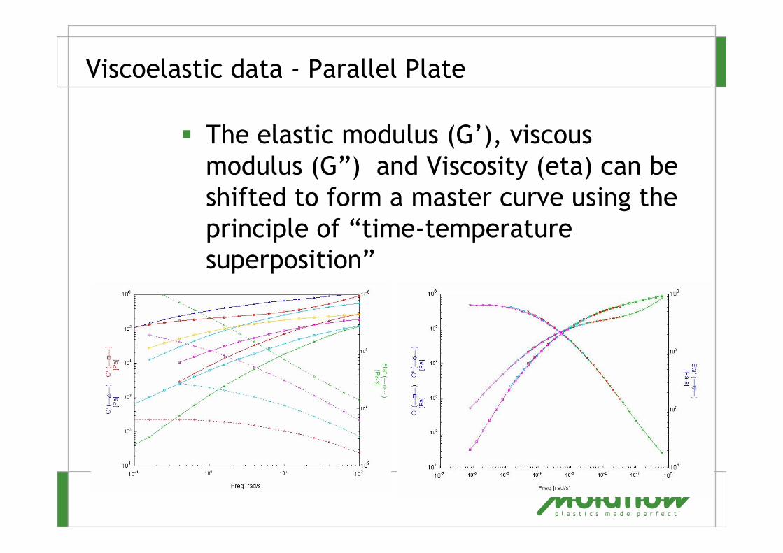
Viscoelastic data - Parallel Plate

� The elastic modulus (G’), viscous

modulus (G”) and Viscosity (eta) can be

shifted to form a master curve using the

principle of “time-temperature

superposition”

Viscoelastic data – Master Curve

� The modulus master curves from the parallel plate and rectangular torsion tests can be combined

at the reference temperature to show the transition from melt to rubber to glass.

Rectangular TorsionParallel Plate

Tref = 140 deg.C

Retardation spectrum

� The modulus (G) master curve can be transformed to the

compliance (J) master curve and then to the retardation

spectrum

Dynamic data Retardation Spectrum

Tref = 140 deg.C

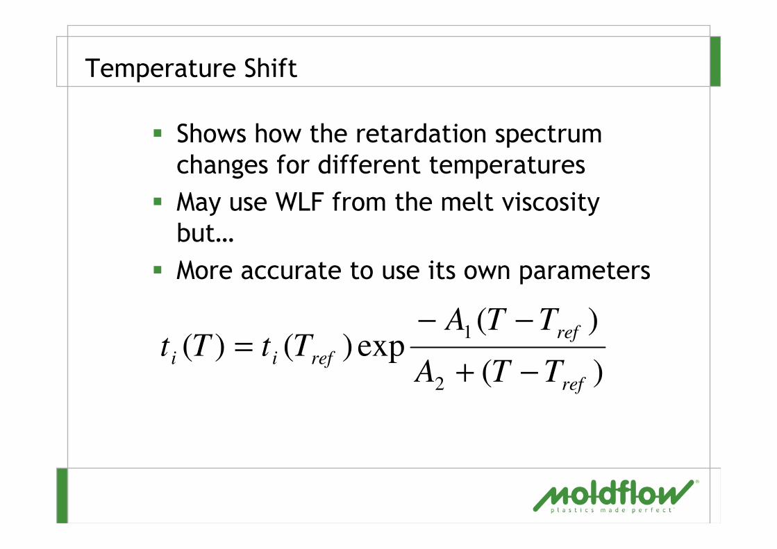
Temperature Shift

� Shows how the retardation spectrum

changes for different temperatures

� May use WLF from the melt viscosity

but…

� More accurate to use its own parameters

)(

)(exp)()(

2

1

ref

ref

refiiTTA

TTATtTt

−+

−−=

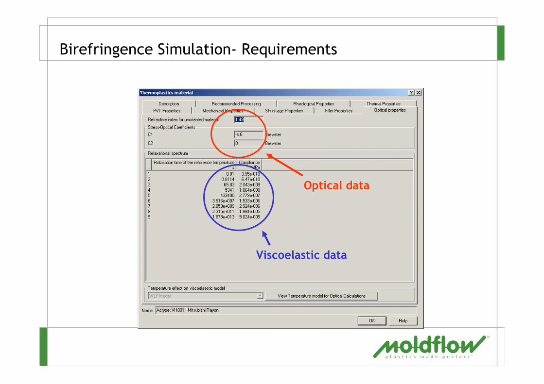
Birefringence Simulation- Requirements

Viscoelastic data

Optical data

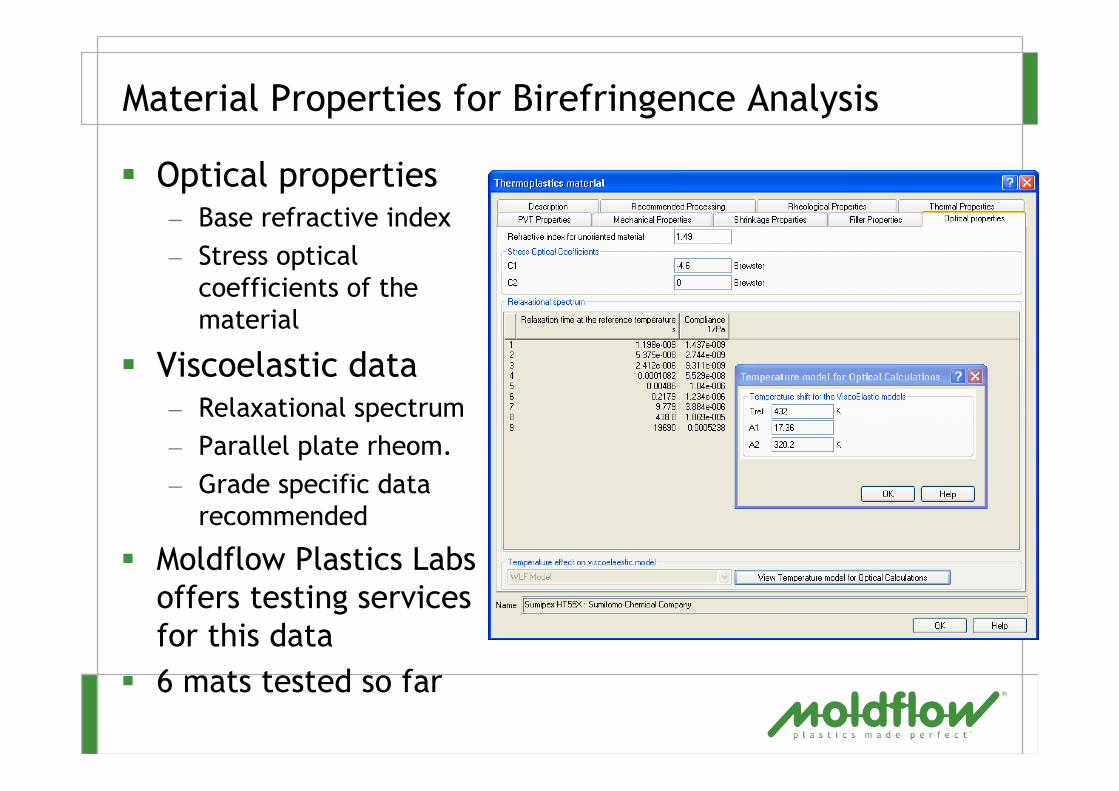
Material Properties for Birefringence Analysis

� Optical properties– Base refractive index

– Stress optical

coefficients of the

material

� Viscoelastic data– Relaxational spectrum

– Parallel plate rheom.

– Grade specific data

recommended

� Moldflow Plastics Labs

offers testing services

for this data

� 6 mats tested so far

Change in Refractive Index

� Difference in refractive index after warpage

� Used to detect changes in refractive index caused by stresses after deformation

Scaled Refractive Index (Cutting Plane)

� Birefringence when tensors in principle directions vary

� Double image– If the change in refractive

index tensor has no axis along the direction of the incident light

� Polarisation effect (color bands)– If one of the axes of the

change in refractive index tensor is parallel to the incident light the polarisation of the light will change.

Retardation

� Difference in horizontally and vertically polarised light expressed in length (nanometers) – Max should be well

under 25% of light wavelength often less (10%)

� Result based on lightdirection

Phase Shift

� Difference in horizontally and vertically polarised light expressed in degrees – Max should be well

under 360º often 90ºor lower is a limit

� Result based on lightdirection

Retardation Measurement Process #1

• Retardation is measured by the Berek compensation technique

• Retardation is measured at 45 points (9x5 grid) offset from cavity edges

• Identical samples are stacked three or more high for greater accuracy

• Reported results are an average for a single sample

Retardation Validation - PMMA

Case 4: 3mm cavity, slow fill

Retardation along Centerline

Maximum Measurement Uncertainty0.72 nm (95% CI)

Reasonable agreement between experiment and MPI

MPI

Experiment

Birefringence Orientation Validation

Experimental Orientation Result for PMMA

Observed direction of maximum birefringence is transverse to flow

Experimental Orientation Result for COP

Observed direction of maximum birefringence is aligned with flow

MPI tensor plots of 1st principal component of retardance tensor

COP

PMMA

n[ ]

R1 R2

Electric dipole

n[ ]

OEle

ctri

c dip

ole

O

Viscoelastic data

� Viscoelastic data is used for

birefringence predictions

� The data allows the simulation of the

evolving refractive index during the

moulding of optical components

� In the future the use of viscoelastic data

is likely to be more widespread

Future Work & Challenges

� Flow of high performance polymers– Liquid Crystal polymers

– Use viscoelastic data to measure response in melt & solid

� Crystallinity effects

� Optical– Birefringence

– Surface finish

� Strength– Performance under load

� Impact resistance

� Electrical

� Effect of colour on shrinkage

� Rapid cooling PVT data

� PVT for Reactive materials