Moisture content profiles and surface phenomena

during drying of wood

Anders Rosenkilde

Doctoral Thesis

BYGGNADSMATERIAL KUNGLIGA TEKNISKA HÖGSKOLAN 100 44 STOCKHOLM

TRITA-BYMA 2002:4 ISSN 0349-5752 ISBN 91-7283-407-2 Trätek Publ 0211038

Moisture content profiles and surface phenomena

during drying of wood

Anders Rosenkilde

I

ABSTRACT Timber drying is one of the most important processes when manufacturing sawn timber products. The drying process influences deformations, surface checking, discoloration and hence, the product quality and the manufacturing costs. Research in this field is of great importance for the wood industry since the industrial drying process always needs to be improved as market demands increases and new wood products are developed. The aim of the present thesis was to investigate the moisture transport behaviour in wood based on measurements during drying from fresh condition down to end use moisture content. The behaviour near the surface interface has been specifically investigated since it is of great importance for the theoretical description of the drying process. Furthermore, studies based on measurements in the wood surface layer during drying are not easy to find in the literature. The reason for that is probably that it is very difficult to make accurate moisture measurements with high spatial or temporal resolution without disturbing the drying process. Measurements of moisture content profiles in Scots pine heartwood and sapwood during drying have been performed by using three different methods. The first was a destructive method where the wood samples are sliced with a knife into several smaller pieces. The moisture content in each piece was determined with the dry weight method. The second method used is non-destructive and it utilises a medical CT-scanner that has been adapted for drying experiments. The samples are dried in-situ the scanner through the whole experiment. The CT-scanner measures density and the moisture content are calculated according to existing methods developed by other scientists. The third method was also non-destructive and it utilises a Magnetic Resonance Imaging, MRI, technique. With this technique the amount of water in the wood sample is measured directly even though it has to be calibrated to moisture content. The surface emission factor, S, or surface resistance, 1/S, has been studied by performing sorption experiments with MDF in a narrow moisture content range. The experiment was evaluated using a simple diffusion model that includes a surface emission factor S. The experimental result was compared with results calculated using well established boundary layer theories. Measurements of moisture content profiles in the wood bulk showed an expected Fickian behaviour at moisture contents below the fibre saturation point. Above the fibre saturation point almost flat moisture profiles were observed. This behaviour was not expected and it is not possible to simulate this behaviour with the existing drying models since they usually assume that there is a gradient in the moisture profile over the whole moisture content range. From the moisture profiles the diffusion coefficients were determined over a moisture content ranging from 8 to

II

30%. The values for heartwood and sapwood are approximately equal in radial and tangential direction to grain. Furthermore, the diffusion values in longitudinal direction are much higher as expected. The sorption experiments with MDF gave a greater surface resistance compared with the calculation that was based on boundary layer theory. The ratio was three or higher. This implied that there was a greater resistance in the surface layer. In addition, this was not well described in the literature even though a few recent published studies exist. High resolution measurements in the surface layer of wood showed behaviour similar to that observed in the bulk wood. The results showed the very early development of a dry zone close to the surface interface. In that zone or shell the moisture content was below the FSP even though the bulk moisture content was far above the FSP. At the end of the experiments the moisture content in the surface layer (0 – 300 µm) nearly reached the equilibrium moisture content even though the bulk moisture content still was much higher. Keywords: Computer tomography, Diffusion, Magnetic resonance, Moisture measurements, Moisture profiles, Surface emission, Wood drying

III

PREFACE Present thesis describes work that has been carried out at Trätek – Swedish Institute for Wood Technology Research. The work has mainly been a part of two projects, namely the Wood physics programme and the Marwingca project. The wood physics programme was a Swedish research programme with several PhD students from different universities in Sweden. It was the first contact with these universities and students that inspired me to start my studies as PhD student at KTH and the department for building material, Paper I-V. The Marwingca project is a European project that initially was planned together with University of Surrey and Dr Paul Glover. There is one person that really has helped me with guidance, inspiration and kept me “on the track” through the years from 1994 to 2002, and that is Dr. Ove Söderström. I am most grateful for his dedicated support. My colleagues at Trätek has been helpful in many ways, Kjell Sjöberg and Vlado Mollek with sample preparation, Bo Edberg with building the experimental kiln, Eva Lindqvist with making this thesis ready for printing and the drying group that has been my inspiring colleagues in the field of wood drying. I am also most grateful for the collaboration with my co-authors Dr. Ove Söderström, Dr. Jesper Arfvidsson, Dr. Paul Glover, Dr. Jean-Phillipe Gorce and Dr. Amanda Barry. They have all been involved in my research for their special and excellent competence. The financial support to the different part of this thesis has come from the Swedish Research Programme Wood Quality, the Institute of Research and Competence Holding AB (IRECO), Swedish National Board for Industrial and Technical Development (NUTEK), Swedish Agency for Innovation Systems (Vinnnova), the European Commission 5th framework programme and the Swedish Wood Association (Svenskt Trä). They are all gratefully acknowledged. Finally I want to thank my wife Ulrika for her support during the years and our children Sixten and Carl Gustaf that has reminded me that there also are other important things in life. Stockholm in November 2002 Anders Rosenkilde

IV

V

CONTENT Page

ABSTRACT I

PREFACE III

CONTENT V

LIST OF PAPERS VII

LIST OF ABBREVIATIONS IX

1. INTRODUCTION 1

2. METHODS FOR MOISTURE PROFILE MEASUREMENTS 2

2.1 Slicing technique 2

2.2 X-ray computed tomography scanning 4

2.3 Magnetic resonance imaging 5

3. MOISTURE PROFILES IN THE WOOD BULK 8

3.1 Materials and methods 9

3.2 Results 9

3.3 Evaluation for determination of diffusion coefficients 14

4. A DRYING SURFACE AND IT’S INTERACTION WITH 16 SURROUNDING AIR

4.1 Materials and methods 17

4.2 Results 19

5. MOISTURE PROFILES IN THE SURFACE LAYER OF WOOD 22

5.1 Materials and methods 22

5.2 Results 23

5.3 Comparison with concrete 29

6. DISCUSSION AND CONCLUSIONS 31

7. FUTURE RESEARCH 33

8. REFERENCES 34

APPENDICES I-VII

VI

VII

LIST OF PAPERS This doctoral thesis consists of the following papers, referred to by their Roman numerals (The author has changed his family name from Samuelsson to Rosenkilde during 1995) 1. Measurement and calculation of moisture content distribution during drying Anders Samuelsson & Jesper Arfvidsson

4th IUFRO International Wood Drying Conference, ”Improving wood drying quality”, Rotorua, New Zealand, 1994, August 9 - 13, 79-86.

II. Measurement and evaluation of moisture transport coefficients during drying of wood

Anders Rosenkilde & Jesper Arfvidsson Holzforschung 1997: 51, 372-380.

III. Measurements of moisture transport coefficients in wood during drying

Anders Rosenkilde & Ove Söderström 5th IUFRO International Wood Drying Conference, “Quality wood drying through process modeling and novel technologies”, Quebec City, Canada, 1996, August 13-17, 523-528.

IV. Measurements of surface emission factors in wood drying Anders Samuelsson & Ove Söderström

4th IUFRO International Wood Drying Conference, ”Improving wood drying quality”, Rotorua, New Zealand, 1994, August 9 - 13, 107-113.

V. Surface phenomena during drying of MDF Anders Rosenkilde & Ove Söderström

Holzforschung 1997: 51, 79-82. VI. High resolution measurement of the surface layer moisture content during

drying of wood using a novel magnetic resonance imaging technique Anders Rosenkilde & Paul Glover Holzforschung 2002: 56, 312-317.

VII Measurement of moisture content profiles during drying of Scots pine using magnetic resonance imaging Anders Rosenkilde, Jean-Philippe Gorce and Amanda Barry Submitted to Holzforschung for publication.

VIII

IX

LIST OF ABBREVIATIONS CT Computer tomography

ESEM Environmental scanning electron microscope

FOV Field of view

FSP Fibre saturation point

MDF Medium density fibreboard

MRI Magnetic resonance imaging

NMR Nuclear magnetic resonance

PTFE Polytetrafluoroethylene

RH Relative humidity

1

1. Introduction Wood drying is an important industrial process in the sawmill industry since it has a great impact on both the product quality and the manufacturing costs. Hence, several scientists have aimed to improve the industrial drying process by developing theoretical models of the drying process: Cloutier et al.(1992); Perré (1996); Arfvidsson (1998); Hukka (1999) and Salin (1999) amongst others. These models need relevant experimental measurements in order to verify their results. A weak point in some of those models has been the description of the moisture transport above the fibre saturation point, FSP, and the behaviour at the surface interface. Usually the models use a moisture potential as the driving force for the moisture transport. Hence, there must be a gradient in the moisture content in the whole moisture content range otherwise the models will calculate zero flux. This drawback has been discussed by Wiberg (2001) and Salin (2002). When wood is drying there is a resistance against moisture transport at the surface which lowers the moisture flux. This resistance, 1/S where S is the surface emission factor, can be described by well established boundary layer theory, Söderström and Salin (1993). If the surface resistance is measured by performing sorption experiments in a narrow moisture content range where the diffusion coefficient can be assumed to be constant, then the measured S-value will be greater than that calculated. This implies that there is a greater internal resistance in the wood surface, which has been reported by Gong and Plumb (1994a, b) and discussed by Kayihan (1993). This effect will be investigated further in this thesis. Recently, Wiberg (2001) has studied drying in sapwood above FSP using a CT-scanner. He showed almost flat moisture profiles in the bulk at moisture contents above FSP. Furthermore, he showed what he called the formation of a dry shell that recedes as an evaporation front towards the bulk. Due to an edge effect in the CT-scanner Wiberg was not able to measure in the surface layer and the resolution, 240 µm, was not high enough. Tremblay (1999) has also shown almost flat moisture profiles above FSP. He used a slicing technique with a resolution down to 380 µm. The aim of the present thesis was to perform measurements during drying of wood in order to accurately describe the actual behaviour and then compare it with theories and calculations for the moisture transport especially near the surface, by using both destructive and non-destructive measurements with low and high resolution. The highest resolution was achieved with the MRI-system, 13 and 21 µm. The system was designed for measurements in planar films and coatings, Glover et al. (1999), and adapted for drying experiments, Rosenkilde and Glover (2002). An advantage with the MRI-system is that it only measures the amount of water. The CT-scanning system measures density in the scanned material. Hence, the measured density is both wood and water. The method for determining the moisture content is described in Lindgren (1992); Rosenkilde and

2

Arfvidsson (1997) and Wiberg (2001). The CT-system was adapted for drying experiments by Wiberg (1998).

2. Methods for moisture profile measurements Three different methods for measuring the moisture content in a piece of wood during drying are used for the measurements that are presented in this thesis. These methods can be divided into two groups, destructive and non-destructive. All these methods have their advantages and disadvantages. The different methods will be briefly described below.

2.1 Slicing technique The slicing technique is a destructive method where the samples were cut with a knife either into ten slices, 29 x 19 x 3 mm3, Figure 1, or cut in a mesh as in Figure 2. Different samples were cut at certain time intervals during the drying period. The moisture content for each slice or piece was determined with the dry weight method. An advantage of the slicing technique is that it is easy to perform and it requires no sophisticated equipment. A well performed measurement gives a low uncertainty. The results showed an uncertainty between ? 0.3% and ? 1.4% moisture content, depending on the number of samples in each measurement batch and the resolution of the balance used. A disadvantage with the slicing technique is that the different measurements during the drying period are performed on different samples since they are destroyed after each measurement. This method presumes that all samples have almost identical moisture transport properties, which could be very hard to achieve even if all specimens originate from a narrow zone in the same log. The slicing technique can only be used when the specimens are dried in tangential or radial direction to the grain and where they were cut along the grain. It is almost impossible to cut the specimen reliably across the grain with a knife. Further details can be found in Paper I to III.

Figure 1. The pattern for slicing the sample into ten lamina. The smaller sample had the following dimensions 29 x 29 x 29 mm3.

Direction of moisture flow during drying

3

The smaller samples were dried in their origin dimension 29 x 29 x 29 mm3 and then cut at certain time intervals. The larger samples were all cut like a 31 mm thick slice out of the same 1200 mm long board and then cut into smaller pieces according to the mesh in Figure 2.

Figure 2. The larger sample, 144 x 50 x 31 mm3, with the pattern for splitting it into rectangular pieces. Each piece had the dimension 31 x 10 x 10 mm3.

2.2 X-ray computed tomography scanning The computed tomography, CT, scanning technology is non-destructive, which allows all measurements to be performed on the same specimen during the whole drying period. The CT scanner uses an X-ray tube and a detector array that rotates around the specimen. The principle of the CT-scanner is more closely described by Herman (1980), Lindberg et al. (1990) and Lindgren (1992). The CT scanner is shown as a schematic in Figure 3. This CT machine measures the transmission of an X-ray beam through the specimen and provides CT-numbers that describe the attenuation of the beam in the measured material. Higher density in the specimen causes greater attenuation of the X-ray beam.

The measured results are provided in a matrix with 512 x 512 pixels. Each pixel represents an area of 0.24 x 0.24 mm2. The CT-numbers for each pixel can be attributed to a wood density according to the algorithm given by Lindgren (1992). Since the dimensions of the specimens were 29 x 29 x 29 mm3, the scanned zone in the specimens consists of approximately 120 x 120 pixels. The X-ray beam had a width of 5 mm and each pixel value represented a measured mean density value for a volume in the specimen

Boundary between sapwood and heartwood

4

with the dimensions 5.0 x 0.24 x 0.24 mm3. Not all of the 120 x 120 pixels are used for measurements because of an edge effect within the image reconstruction algorithm, which causes problems with inaccuracy up to 2 mm from the edges. Hence, the part of the measured area used in the specimen consisted of 100 x 80 pixels, which is equal to 24 x 19 mm2, Figure 4.

Specimens

Climate chamber

Rotating detector array

Rotating X-raytube

Figure 3. The computed tomography, CT, scanner with the climate chamber and test samples in the scanning zone.

Measured area 24x19 mm2

Direction of flow

Dried surface

29 mm

29 m

m

5 mm, width of X-ray beam

5 mm

29 mm

5

Figure 4. The scanning zone in the test sample and the ten mean value areas used in the measurements.

This area was divided into ten smaller areas with 10 x 80 pixels. The mean density for each of those areas provides a density gradient with ten values in the direction of the moisture flow. From the density profiles, moisture content profiles were calculated according to Lindgren (1988). This analysis requires a calibration density measurement to be made at known moisture contents. At the end of the experiment the specimens were equalized in the climate chamber at the constant climate used during the drying period. After this moisture content equalization, the specimens were CT-scanned. This provided an almost constant density, i.e. with no gradient in the scanned zone. After this last CT-image, the scanned zone was immediately cut out of the specimen and its moisture content was evaluated with the dry weight method. The mean density of the measured zone and the moisture content of the same zone were used as a reference when calculating the moisture content gradients in all the other measurements. Further details can be found in Paper II.

2.3 Magnetic resonance imaging Magnetic Resonance Imaging (MRI) is a Radio-Frequency (RF) spectroscopic method based on the magnetic properties of the investigated material or more precisely the investigated nuclei. In the case of wood and moisture content measurements it is the hydrogen nuclei we are interested in. When a piece of wood is placed in a uniform magnetic field, B0, the spin of the hydrogen nuclei (a single proton) align with the magnetic field. If we apply an oscillating RF magnetic field pulse that is perpendicular to the main field B0 the spin of the protons tip 90o so they align with the RF field. After this pulse the spins relax back to their equilibrium state to align with the main field again. While this happens they emit energy in the form of a radio signal which can be detected with a coil. The intensity of that signal is proportional to the amount of hydrogen protons or amount of water. The frequency of the signal from the protons at resonance is called the Larmor frequency which is defined as, ? = ?B0 (1)

where ? = Larmor frequency (radians s-1), ? = the gyromagnetic ratio and B0 the main field (T). In the MRI system used in this study there is also a gradient in the main magnetic field. According to Equation (1) the resonance frequency from the protons in the studied material varies with the position or strength in the main field. This gradient then gives spatial information so the moisture profile can be detected. Further information about the principles of MRI can be found in Callaghan (1991).

6

The MRI equipment used was a novel high-gradient permanent magnet that was originally designed for profiling through thin planar films and coatings. The probe used for these studies as shown in Figures 5a and 5b consists of a sample holder made of PTFE with a built-in RF coil. The diameter of the RF coil was 10 mm and was tuned to 30 MHz. The probe assembly fits between the magnet pole -pieces so that the edge of the wood sample inside the probe was situated at the correct magnetic field during the experiment.

Figure 5a. Sample holder and RF probe, seen from the long side.

80 mm

55 m

m

? 15 mm

Wood sample

RF coil

Air inlet Air outlet

Measured zone 1.5 mm gap

7

Figure 5b. Sample holder and RF probe, located between the curved permanent magnet pole-pieces. The magnetic field strength at the sample surface is 0.7 T (Tesla) and was nominally parallel to the wood surface. A field gradient of 17 Tm-1 exists vertically (normal to the wood surface), which is employed to give a very high spatial resolution in this direction only. There is a slight downward force on the sample to ensure that the surface does not move during drying. Between the wood surface and the RF coil there was a 1.5 mm gap where a climate controlled airflow transports away the water that evaporates from the wood surface. The RF coil is only sensitive in a narrow zone near the coil, therefore, the gap between the coil and the wood sample needs to be as small as possible. It is estimated that when the probe was used with the available RF pulse power (12 W), the measured zone in the wood had a diameter about 5 mm. The achieved spatial resolution in the experiments was 13 and 21 µm with a field of view of 300 and 600 µm. In the experiments performed, two different air velocities were used, 1.9 m/s (Scots pine heartwood and concrete) and 3 m/s (Scots pine sapwood). These air velocities are comparable with air velocities of approximately 8 and 12 m/s in an industrial kiln where the air gap between the drying wood surfaces commonly is around 25 mm compared to the 1.5 mm air gap in the experiments. Comparable air velocities correspond to equal heat transfer coefficients for both 1.5 and 25 mm air gaps. By using the defination for Nusselt, Equation 2, and Reynolds number, Equation 3, and stating that the proportionality between Nu and Re0.67 should be constant with both the 1.5 and 25 mm air gaps, the relationship between the air velocities can be calculated.

NdFeB magnet

Pole pieces

RF coil ? 10 mm

Measured zone ? 5 mm

Air inlet/outlet

Wood sample

8

Nu = ad/? (2)

Re = vd/? (3)

Where a = heat transfer coefficient (W/m2K), d = air gap (m), ? = heat conductivity in air (W/mK), v = air velocity in air gap (m/s) and ? = kinematical viscosity (m2/s). In Re0.67

the correlation factor 0.67 is established experimentally, Söderström (1987). Normal air velocities in industrial kilns are from 2 m/s to 5 m/s. Further details about the MRI equipment can be found in Paper VI.

3. Moisture profiles in the wood bulk The aim of measuring the moisture content profiles in the bulk was to determine the diffusion coefficients for Scots pine sapwood and heartwood in all three directions relative to the grain. The result was meant to be used for verifying wood drying models. Another aim with the measurements was to evaluate two different experimental methods for obtaining the moisture content profiles.

9

3.1 Materials and methods In the experiments the moisture content profiles were measured in Scots pine (Pinus sylvestris) at different times during the drying period. Two kinds of measuring methods were used, destructive and non-destructive. The destructive method, slicing technique, was used on both smaller (30 x 30 x 30 and 29 x 29 x 29 mm3) and larger (144 x 50 x 31 mm3) wood samples, Papers I and II. The non-destructive method, CT-scanning, was used for the smaller samples (29 x 29 x 29 mm3), Paper II. All small samples were made of either heartwood or sapwood, the larger samples contained both sapwood and heartwood. In the case of the smaller samples two opposite sides were in contact with the airflow, all other sides were sealed and insulated. Therefore, these measurements gave profiles from surface to surface but they were presented as centre of the specimen to the surface. Hence, the presented profiles were mean values of the two profiles from the centre of the specimen towards both surfaces. Since the specimens are divided into ten areas, there is no measured value for the centre of the specimens. Therefore, the centre value here was estimated with a mean value for the two nearest measurements on either side of the centre. 3.2 Results The results from the destructive measurements with the larger samples can be found in Paper I. The results that are presented here are those for smaller samples (29x29x29 mm3) where the moisture content profiles were measured in the radial and tangential direction using the slicing technique and the CT-scanning technique for measurements in the longitudinal direction. Further details can be found in Paper II and III. Heartwood The results from the destructive and non-destructive measurements on the smaller samples of Scots pine heartwood are shown in Figures 6 and 7. In Figure 6 the moisture content profiles show similar behaviour for both drying in the radial and tangential direction. Since the moisture content starts nearly at FSP, a gradient starts to develop from the surface and towards the bulk from the beginning. Therefore, the moisture transport process is here mainly a diffusion process.

10

Figure 6. Measured moisture content profiles using the slicing technique in Scots pine heartwood, dried in radial direction to grain to the left and in tangential direction to the right. Both dried at 60 oC and 59% RH. The surface is towards right on the distance axis. In Figure 7, where the result from drying Scots pine heartwood in the longitudinal direction to grain is presented, the same behaviour can be observed as in Figure 6. The main difference between the moisture profiles in Figures 6 and 7 is the time. Scots pine heartwood dried much faster in the longitudinal direction to grain than in radial or tangential, in the longitudinal direction the wood sample reached equilibrium moisture content within 16 hours of drying, even in the bulk.

5

10

15

20

25

30

35

0 2 4 6 8 10 12 14

Distance from centre [mm]

MC

%

0 h

8,6 h

20,3 h

26,4 h

32,7 h

43,2 h

54,6 h

95,1 h

5

10

15

20

25

30

35

0 3 6 9 12

Distance from centre [mm]M

C %

0 h

4,4 h

16,3 h

22,2 h

28,5 h

39,0 h

90,5 h

11

Figure 7. Measured moisture content profiles using the slicing technique in Scots pine heartwood dried in longitudinal direction to grain at 60 oC and 59% RH. The surface is towards right on the distance axis. The measured moisture content near the surface, Figure 7, increases at the end of the drying period. This could be caused by the extractives in heartwood that migrate to the surface which the CT-scanner observes as an increase in density and render as moisture content. A similar observation has been made by Morén (1987) in specimens with extreme amounts of extractives. Terziev et al. (1993) have done measurements of extractives that migrate towards the surface during drying of Scots pine. Sapwood As for heartwood the moisture profiles in Scots pine sapwood are presented in all three directions to grain, Figures 8-10. In these figures the moisture content profiles decrease from the centre of specimen towards the surface when the moisture content is approximately below FSP. According to Siau (1984) the FSP is approximately 27% at 60 oC. Furthermore, Figures 8 and 9 show that only one or two measurements were performed during drying above FSP. This is due to fast drying above FSP and also to an accuracy problem with the slicing technique at high moisture content levels in thin samples. Consequently this work has concentrated the measurements in the region below FSP except in the case with longitudinal drying where the CT scanner was used, Figure 10.

5

10

15

20

25

30

35

0 2,4 4,8 7,2 9,6 12

Distance from centre [mm]

MC

%0 h

2,3 h

3,1 h

4,0 h

6,0 h

7,0 h

9,2 h

15,9 h

12

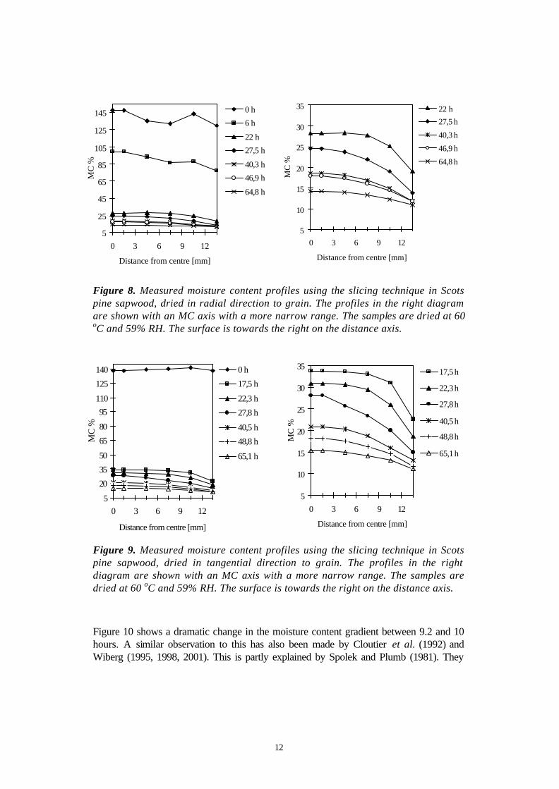
Figure 8. Measured moisture content profiles using the slicing technique in Scots pine sapwood, dried in radial direction to grain. The profiles in the right diagram are shown with an MC axis with a more narrow range. The samples are dried at 60 oC and 59% RH. The surface is towards the right on the distance axis.

Figure 9. Measured moisture content profiles using the slicing technique in Scots pine sapwood, dried in tangential direction to grain. The profiles in the right diagram are shown with an MC axis with a more narrow range. The samples are dried at 60 oC and 59% RH. The surface is towards the right on the distance axis. Figure 10 shows a dramatic change in the moisture content gradient between 9.2 and 10 hours. A similar observation to this has also been made by Cloutier et al. (1992) and Wiberg (1995, 1998, 2001). This is partly explained by Spolek and Plumb (1981). They

5

25

45

65

85

105

125

145

0 3 6 9 12

Distance from centre [mm]

MC

%

0 h

6 h

22 h

27,5 h

40,3 h

46,9 h

64,8 h

5

10

15

20

25

30

35

0 3 6 9 12

Distance from centre [mm]

MC

%

22 h

27,5 h

40,3 h

46,9 h

64,8 h

5

20

35

50

65

80

95110

125

140

0 3 6 9 12

Distance from centre [mm]

MC

%

0 h

17,5 h

22,3 h

27,8 h

40,5 h

48,8 h

65,1 h

5

10

15

20

25

30

35

0 3 6 9 12

Distance from centre [mm]

MC

%

17,5 h

22,3 h

27,8 h

40,5 h

48,8 h

65,1 h

13

state that there is a certain saturation where the liquid phase continuity is disrupted and liquid flow caused by capillary pressure is no longer possible as a moisture transport process. This is called the irreducible saturation. Below the irreducible saturation the moisture transport is mainly a diffusion process, which can be described by Fick´s law (4).

g Dux

? ? ???

? (4)

where g is the moisture flux (kg/m2s), u is the moisture content (kg/kg), x is distance (m) and ? is the wood density (kg/m3). According to Equation (4) the moisture flux g increases with an increasing gradient in moisture content, ? ?u x . An increased gradient gives an increased inclination in the moisture content profiles. Further, if the gradient ? ?u x is equal to zero the moisture content profiles are flat and horizontal. Above a moisture content of approximately 30% the profiles are nearly flat and horizontal. According to Equation (4) the moisture flux g should be nearly zero, but quite opposite it is very high. An explanation to this behaviour is given by Wiberg (1995) that concludes that the free water in sapwood migrates due to capillary forces towards the surface where bound water diffusion controls the drying rate.

Figure 10. Measured moisture content profiles using the slicing technique in Scots pine sapwood, dried in longitudinal direction to grain. The profiles in the right diagram are shown with an MC axis with a more narrow range. The samples are dried at 60 oC and 59% RH. The surface is towards the right on the distance axis.

5

20

35

50

65

80

95

110

125

0 2,4 4,8 7,2 9,6 12

Distance from centre [mm]

MC

%

0 h0,3 h2,3 h3,1 h4,0 h6,0 h6,9 h7,9 h9,2 h10,0 h11,0 h12,0 h13,9 h15,9 h

5

10

15

20

25

30

35

0 2,4 4,8 7,2 9,6 12

Distance from centre [mm]

MC

%

9,2 h

10,0 h

11,0 h

12,0 h

13,9 h

15,9 h

14

3.3 Evaluation for determination of diffusion coefficients The method for the evaluation and determination of diffusion coefficients from the measured moisture content profiles was what is called the Kirchhoffian moment integral method, Paper II, Claesson and Arfvidsson (1992). This method is based on the use of Kirchhoff flow potential, Equation (5).

? ? ?D dwww

w

ref

(5)

The Kirchhoff potential ? (kg/ms) is the area under the diffusion curve Dw(w) (m2/s) between the moisture contents wref and w (kg/m3), Figure 11. The relationship between the Kirchhoff potential and the diffusion coefficient is given by Equation (6), which is the derivative of the Kirchhoff potential ? with respect to w.

Dddww ??

(6)

A complete description of the Kirchhoff potential and Kirchoffian moment method can be found in Paper II.

Figure 11. The Kirchhoff potential ? is the area under the diffusion curve Dw(w) between the moisture contents wref and w (kg/m3).

Dw(w)

?

w wref w

15

The method of evaluation described above resulted in diffusion coefficients Dw and their dependence on the moisture state. In Table 1 the diffusion coefficient Dw is given for sapwood and heartwood in radial, tangential and longitudinal direction to grain. The D-values are given in a range of moisture contents from 8 to 30%. Table 1. The diffusion coefficient Dw at 60 oC for Scots pine sapwood and heartwood in all three directions to grain: radial, tangential and longitudinal.

Sapwood Heartwood long. MC %

D?1010

m2/s

tan. MC %

D?1010

m2/s

rad. MC %

D?1010

m2/s

long MC %.

D?1010

m2/s

tan. MC %.

D?1010

m2/s

rad. MC %.

D?1010

m2/s

8.3 30 11.6 7.6 11.1 5.0 11.7 25 10.8 6.2 10.8 5.0

10.1 35 13.2 7.5 13.2 7.5 13.5 30 12.8 6.3 12.8 6.2

12.0 35 15.2 8.7 15.2 10 15.3 30 14.8 7.5 14.8 6.3

13.8 35 17.2 10 17.2 10 17.1 30 16.8 8.7 16.8 7.5

15.7 35 19.2 10 19.2 15 18.9 30 18.7 8.8 18.7 7.5

17.5 35 21.3 14 21.3 18 20.7 35 20.7 10 20.7 10

19.4 40 23.3 13 23.3 30 22.5 35 22.7 8.7 22.7 9.2

21.2 35 25.3 13 25.3 28 24.3 40 24.7 8.8 24.7 12

23.1 40 27.3 10 26.6 40 26.1 30 26.6 13 26.6 14

24.9 40 28.8 15 27.9 30 28.6 15 28.6 18

26.8 60 29.7 30 30.1 25

28.6

30.0

In Figure 12 all D-values from Table 1 are plotted versus the moisture content. The values for heartwood and sapwood in radial and tangential direction to grain are approximately equal. It is only the D-values for sapwood radial that are higher at moisture contents above 17 to 18%. According to Morén (1987) and Malmquist (1990, 1991), the mean diffusion coefficient for Scots pine heartwood and sapwood in radial and tangential direction to grain is 7.1 ? 10-10 and 5 to 8 ? 10-10 m2/s respectively at 60oC, a heartwood percentage of 73% and a mean moisture content of 13.5%. If the same mean diffusion coefficient is calculated using the D-values from this work the result is 6.9 ? 10-10 m2/s. This result shows very good correspondence. The D-values in longitudinal direction are much higher as expected, but the values are almost equal in the whole moisture content range except the values in sapwood, which increase dramatically when the moisture content is above 25 to 27%. Even though the moisture transport process is not a diffusion

16

process above the FSP, the diffusion coefficient was used here to characterize the moisture transport process in the whole moisture content range.

Figure 12. The diffusion coefficient Dw versus the moisture content for Scots pine sapwood and heartwood in all three directions to grain, radial, tangential and longitudinal. The graph to the right has a more narrow range on the diffusion axis.

4. A drying surface and it’s interaction with surrounding air

Experiments have been made with the purpose to demonstrate the influence of the surface interaction with the surrounding air on the moisture flow in Medium Density Fibreboard, MDF. The measurements were performed as sorption experiments, a constant humidity abruptly being changed isothermally to a lower constant humidity. The moisture content response of MDF-board samples with six different thicknesses was measured over time. The analysis of the experiments was done by using a mathematical method including a simple diffusion model with constant diffusion coefficient and surface emission factor. The aim with the analysis was to determine the surface emission factor from the experiments and compare it with a theoretical calculated value according to boundary layer theory. 4.1 Materials and methods Seven samples of MDF were conditioned in a climate chamber at 56 oC and relative

0

20

40

60

80

100

120

0,05 0,15 0,25 0,35

MC (kg/kg)

Dw

(m2 /s

) x 1

010

s.long

s.tan

s.rad

h.long

h.tan

h.rad

0

10

20

30

40

0,05 0,15 0,25 0,35

MC (kg/kg)

Dw

(m2/s

) x 1

010

s.tan

s.rad

h.tan

h.rad

17

humidity RH 95%. After the samples had reached the equilibrium moisture content they were moved quickly to an experimental kiln, Paper IV. To ensure that the samples had reached equilibrium moisture content, they were kept in the climate chamber until the weight was stable, which took at least 14 days. In the experimental kiln the climate was 56 oC and RH 61%. The average air velocity in the kiln was 3 m/s. The equilibrium moisture contents in the climate chamber and the kiln were estimated by using 2 mm thin flakes of MDF as moisture content samples. These flakes were placed alongside the test pieces during the experiments. Not all of the thicker samples reached equilibrium moisture content during the drying phase, therefore, the thinner MDF flakes were used. The moisture content in the thin flakes was estimated with the dry weight method. All samples of MDF had the following dimensions: width 150 mm, length 940 mm and thicknesses, 13, 16, 21, 27, 31, 35 and 46 mm. The reason for using MDF instead of solid wood was that the evaluation of the measurements presupposes that the sample properties are identical and homogeneous in all samples. This is difficult to achieve with solid wood. The density profile in the MDF samples along the thickness was measured with a gamma-ray density meter. These measurements showed a high density in the surface layers of the original 56 mm MDF-board. Hence, all pieces were cut from the centre part of the original MDF-board to ensure a flat density profile and identical properties in all test samples. Further details about the experiment can be found in Paper IV. The data sets from the sorption experiments were interpreted as a simple diffusion model, Equation 7, with a surface emission factor included, Equation 8, Paper IV. Namely:

2

2u u

Dt x

? ??? ?

(7)

where u is the moisture content, t the time, D the diffusion constant and x the space coordinate. The boundary condition is given by:

(8)

where ueq is the equilibrium moisture content for wood in the ambient air, subscript “a” refers to the value at the surface and S is the surface emission factor (m/s). The relative mean moisture content is defined by:

(9)

- [ ( - )] a eqauD S u ux

? ??

0

0 eq

-uuF=-u u

18

where u is the mean moisture content, u0 is the initial moisture content. The quantity F is determined by continuous registration of the weight over time. By plotting F vs. t0.5 an initial straight line is expected if the process is solely described by a constant diffusion coefficient. An initial time lag is interpreted as the existence of an internal resistance in the surface, here described as 1/S. F starts from zero and approaches 1 in time. The time when F = 0.5 is denoted t0.5 and this quantity is connected to D and S by:

(10)

where a is half the material thickness. (Söderström and Salin 1993), Paper V. When sorption experiments are performed with different thicknesses the quantity t0.5/a2 can be plotted vs. 1/a. Equation 10 is an approximate formula, but can be used as a first attempt, Paper V. With the experimental data t0.5/a2 versus 1/a, a regression analysis with weighted data points is made with the weight function 1/(s(t0.5/a2))2, where s(t0.5/a2) is the standard deviation for t0.5/a2. The regression analysis gives the regression parameters A = 0.2/D, which is the intercept, and B = 0.7/S, which is the inclination. The diffusion coefficient D and the surface emission factor S were calculated with the regression parameters and Equation 10. These results were compared with results from the more accurate non-linear description by Söderström and Salin (1993). In all seven data points in Figure 14 the error in measurement was estimated with the standard deviation s(t0.5/a2). This standard deviation includes both the inaccuracy of balance and the sliding calliper. The balance were used to weigh the test samples, and the sliding calliper was used to measure their thicknesses. 4.2 Results In Table 2 the experimental data and results are presented for all seven experiments. The spread in moisture content u0 was caused by the inaccuracy of the control system for the climate chamber. Hence, it was necessary to check the equilibrium moisture content in the climate chamber with the 2 mm thin MDF flakes. The moisture content ueq had much less spread because the kiln climate was easier to control and the control system was specially designed for this purpose. The standard deviation s(t0.5/a2) increases with decreasing thickness, due to the inaccuracy in the balances and the sliding calliper, which causes greater errors for lighter and thinner samples. On the other hand, the standard deviation s(t0.5) decreases with decreasing thickness. This is caused by an increase in inclination in

0.52

0.2 0.7t = +D Saa

19

the plot F versus t0.5 with decreasing thickness. With the measured D and S-values, F versus t0.5 was calculated for all seven experiments. In Figure 13 both calculated and measured values of F versus t0.5 are plotted for MDF with thickness 13 mm. The calculation of F is described by Söderström and Salin (1993).

20

Table 2. Experimental data and results when drying Medium Density Fibreboard, MDF, with different thicknesses from moisture content u0 to ueq. a u0 ueq t0.5 t0.5/a2 s(t0.5) s(t0.5/a2) [m] [%] [%] [s] [s/m2] [s] [s/m2]

0.0230 21.0 9.4 50 500 0.96·108 5 200 0.14·107

0.0177 19.8 9.4 31 500 1.01·108 3 000 0.19·107

0.0155 21.1 9.4 25 500 1.06·108 400 0.22·107

0.0135 20.0 9.4 20 200 1.11·108 2 000 0.27·107

0.0108 21.7 9.8 14 100 1.21·108 1 000 0.37·107

0.0080 19.5 9.4 9 300 1.45·108 900 0.60·107

0.0065 20.3 9.8 6 900 1.63·108 700 0.82·107 F t0.5 Figure 13. F versus t0.5 , the smooth line is calculated with the half thickness a = 0.0065 m, D = 2.9 · 10-9 m2/s and S = 1.2 · 10-6 m/s. The other line is experimental data for MDF with thickness 13 mm. In Figure 13 an initial time lag can be observed in the measured and calculated F versus t0,5 curves. This is due to the resistance in the surface layer, 1/S. If the curves had started

0,00

0,20

0,40

0,60

0,80

1,00

0 100 200 300 400 500 600

21

without a time lag they would have been straight and then the resistance in the surface layer could have been neglected. In Figure 14 Equation 10 is plotted with confidence limits and data points including error bars. The more accurate non-linear, Söderström and Salin (1993), dashed line is almost within the confidence limits in the whole measured interval. Hence, the approximation with Equation 10 can be used in this case. The regression analysis gave the regression parameters A = 69590000, which is the intercept, and B = 573600, which is the inclination. This gave the diffusion coefficient D = 2.9·10-9 m2/s and the surface emission factor S = 1.2·10-6 m/s. Both D and S are in the same magnitude as reported earlier ( Choong and Skaar 1969, Koponen 1988). t0.5/a2 1/a Figure 14. t0,5/a2 vs 1/a. The squared dots are measured values from all seven experiments, the thick straight line in the middle is the weighted regression line to the seven measurements, two outer solid lines show the 95% confidence limits to the weighted regression line and the dashed line is calculated with a non-linear model described in the text. For comparison a calculated value of the resistance at the surface was calculated by using Equation 11, Paper V.

(11)

9,0E+7

1,1E+8

1,3E+8

1,5E+8

1,7E+8

40 80 120 160

--

a e qsT

p a e qa i r

h hS

w o o dc u u

? ???

? ?

22

where a is the heat transfer coefficient (W/m2K), ?sT is the saturation moisture concentration in air at temperature T (K), cp is the heat capacity in the air, ?air is the density of the air (kg/m3), ?wood the density of wood defined as dry mass over raw volume (kg/m3), h the relative humidity and u moisture content. Subscript “a” refers to the value at the surface and “eq” to the value that is in equilibrium with the ambient air. The calculations resulted in S-values that varied from about 4 to 17 ·10-6 m/s, depending on the inclination of the sorption curve. These calculated S-values are 3 to 14 times higher than the measured value. This has also been observed by Gong and Plumb (1994a, b). The calculated surface resistance 1/S represents only the external surface resistance, which is well described by boundary layer theory, Paper V. Since the measured surface resistance 1/S is higher than the calculated the measured value probably describes both the external resistance and a greater internal resistance in the surface layer. This fact has also been described by Kayihan (1993); Wiberg and Morén (1999); Wiberg et al. (2000) and Salin (2002).

5. Moisture profiles in the surface layer of wood High resolution moisture content profiles have been measured during drying in the surface layer (0 – 300 µm) of Scots pine sapwood and heartwood. For comparison measurements have also been performed with samples of concrete. The aim with the surface layer measurements was to investigate the moisture behaviour at the surface interface since it was concluded in Paper V that the measured surface resistance, 1/S, consists of two parts: classic external surface resistance, described by well understood boundary layer theory (Söderström and Salin 1993), and a greater internal resistance in the surface layers that not in general has been well described, presumably because it is difficult to measure the moisture content profiles near the surface interface. Lately Wiberg (2001); Rosenkilde (2002) and Salin (2002) have been investigated the internal resistance at the surface. Wiberg (2001) called the behaviour at the surface “dry shell formation”, he also made measurements of moisture content profiles but not with as high resolution as in this present work. Salin (2002) concluded that the dry shell at the surface explains the difference between the measured and calculated surface resistance, 1/S. 5.1 Materials and methods Three experiments were performed; the first used two samples of Scots pine (Pinus sylvestris) sapwood, which originated from Dala-Järna in Sweden. These samples were shaped as small round cylinders with a diameter of 14 mm and a length of 20 mm. They were cut out with the radial direction along the length axis of the cylinder. In the second experiment one sample of Scots pine (Pinus sylvestris) heartwood was used which originated from the district around Söderhamn in Sweden. The heartwood sample was cut out in the same way as the sapwood samples with 14 mm diameter and a length of 25

23

mm. For comparison, a third experiment was performed with a sample of concrete, standard Portland cement and sand with a proportion of water/cement around 0.6. The concrete sample were shaped as a cylinder with a diameter of 14 mm and length of 40 mm. During the experiments all samples were dried from wet condition. The wood samples were in fresh condition with moisture contents of 116% (sapwood) and 70.5% (heartwood). The concrete sample was hardened and then rewetted in liquid water to a moisture content of 5.3% before the experiment started. Further details about the materials can be found in Paper VI and VII. During the first experiment with Scots pine sapwood the temperature was between 43 oC and 46 oC and a relative humidity between 16% and 18%. During the second and third experiment the temperature was 22 oC and the relative humidity was 57% except at the end of the second experiment with heartwood where the relative humidity was raised to nearly 100%. The air velocity was in the first experiment 3 m/s and in the second and third it was 1.9 m/s. Further details about the parameters in the experiments can be found in Paper VI and VII. 5.2 Results The analysed results from the measurements on Scots pine sapwood and heartwood are presented in Figures 15 and 17–19. The surface interface of the sample is assumed to be at 0 µm on the distance axis in Figures 15, 17 and 18. Due to resolution broadening the sample interface was not exactly at 0 µm. The sample interface was in the measurements more like a thin zone due to three factors, the first being sample alignment. The sample was never exactly aligned with the magnetic field. This gives a measured zone that contains both of sample material and air. The proportion of air in that zone increases with distance from the bulk. This affects the signal profile in a way that it will decay as the proportion of material decreases. The second factor is the roughness of the surface that will have the same effect on the measured profile as the sample alignment. The roughness of the surface is of the same magnitude as the diameter of a wood cell, Figures 16 and 20. The third factor is the shift between the sample surface and the end of the last pixel. The pixel size is 13 or 21 µm. This factor will also affect the signal profile since the sample surface will not end exactly where the pixel ends. Therefore, the last pixel containing signal from the sample material will contain both sample material and air which will lower the measured signal in the last pixel, resulting in an observed decay in the measured profile. Sapwood From the moisture content profile in Figure 15, it can be observed that the profiles from 0.5 h to 4 h are almost flat without a gradient from a depth of 90 ?m and further in. Furthermore, a steep gradient can be observed in those profiles from the surface to the

24

depth of 90 ?m. This indicates that the sample has dried a little during preparation of the experiment. Wiberg (1998) and Tremblay (1999) have also reported steep gradients near the surface at moisture contents above FSP. Their “dry shell” with the steep gradient was about 2 to 3 mm from the surface compared to 0.1 mm in this study. An explanation of that could be the difference in roughness of the wood surface. Wiberg (1998) and Tremblay (1999) used samples with sawn surfaces obtained from industrial production, whereas for this study, the surfaces were first sawn and then cut with a microtome resulting in a flat smooth surface. The shape of the actual sample surface can be seen in Figure 16, which is an Environmental Scanning Electron Microscope, ESEM, image. In the image, the roughness is about the size of a cell or less. The size of the cells is around 25 ?m. This should be compared with a sawn surface where the roughness probably is around 0.5–1 mm. A more likely explanation of the difference between the present results and others is that it is a matter of resolution and field of view.

Figure 15. Moisture content profiles for Scots pine sapwood dried at 43 oC to 46 oC with a relative humidity of 16% to 18%, ? o? 0.5 h, ? x? 1 h, ? ? ? 2 h, ? ? ? 4 h, ? ?? 7 h, ? ? ? 19 h, ? +? 24 h.

0

2 5

5 0

7 5

100

125

150

0 52 104 156 208 260

Distance (µm)

Moi

stur

e co

nten

t %

25

Figure 16. ESEM image of a part of the measured zone in the Scots pine sapwood sample. The image shows the wood structure across the grain and the axis shows the field of view in the measurement, magnification 145x. In this image it can be observed that the measurements have been made in the late wood. In Figure 16 it can be observed that the measured zone consisted of only late wood, which has a higher density and lower diffusion coefficient than the early wood. The field of view of the MRI measurement is marked in Figure 16 with an axis. The accuracy in the moisture content profiles for sapwood is dependent upon the method for calibration and normalisation of the measured signal to moisture content. Since the NMR signal decreases with distance from the surface and the transmitting coil, each profile has to be normalised using a known moisture profile. We used the initial profile, measured at raw condition before the drying started. That profile is assumed to be flat at a constant moisture content of 116%. The raw moisture content was measured in a twin sample by using the dry weight method on a 2 mm thick slice from the surface. The twin sample had the same origin and the same preparation and storage. The moisture profiles show the subsequent relative changes compared to the initial profile. Therefore, the accuracy in moisture content is very much dependent on the first profile, both the accuracy in value and how flat the profile was at raw conditions. However, this method of using the first profile to normalise the other profiles causes an uncertainty in the resulting profiles.

0 ?m

100 ?m

200 ?m

300 ?m

27

Heartwood The measured moisture content profiles are presented in Figures 17 and 18. In Figure 17 it is clearly seen that a lot of water ingress has taken place during storage in the sealed partly water filled plastic bags before the measurement started. The high amount of water close to the surface evaporates very quickly, after 9 minutes of drying the moisture profile is almost flat. The moisture profiles stay almost flat down to a moisture content slightly above 30% at 41 minutes of drying where a gradient starts to develop at the surface, Figure 18. The profiles recorded after 41 minutes show all a gradient from the surface interface towards the bulk. This behaviour with almost flat profiles above a moisture content of approximately 30% and a gradient developing from the surface at lower moisture contents has been reported before, Rosenkilde and Arfvidsson (1997); Tremblay et al. (2000); Wiberg (2001); Rosenkilde and Glover (2002) and Salin (2002). The development of the mean moisture content in the measured zone can be observed in Figure 19. It is clearly seen that the moisture in the surface layer (0 – 300 µm) evaporates very quickly and then sets at a nearly constant moisture content level. At the end of the drying period the climate is changed to wetter conditions and the moisture content is increasing a lot. At the end of the experiment, the relative humidity is 100% and therefore water condensation occurs at the sample surface. This can be seen in the moisture profile recorded at 1347 minutes in Figure 18. A steep gradient with moisture content clearly above the fibre saturation point is detected at the surface interface. Without condensation at the surface interface, the moisture content never exceeds the fibre saturation point. During the whole drying period the moisture content in the bulk changes from 70.5% to 53.4% which implies that there is a moisture flow going through the relative dry wood surface.

28

Figure 17. Moisture content profiles in Scots pine heartwood during drying. The actual surface is at 0 µm on the distance axis, ? ? ? 0 min, ? ¦ ? 5 min, ? ? ? 9 min, ? *? 16 min, ? ?? 41 min, ? +? 56 min, ? ? ? 1254 min. Figure 18. Moisture content profiles in Scots pine heartwood during drying and conditioning, enlarged version of Figure 17 with a more narrow moisture content range. The actual surface is at 0 µm on the distance axis, ? ? ? 9 min, ? *? 16

0

25

50

75

100

125

150

175

200

225

250

275

-100 0 100 200 300 400 500Distance (µm)

Moi

stur

e co

nten

t %

0

100

200

300

400

500

600

700

800

Moi

stur

e co

nten

t (kg

/m3)

0

20

40

60

80

100

120

-100 0 100 200 300 400 500

Distance (µm)

Moi

stur

e co

nten

t %

0

50

100

150

200

250

300

350

Moi

stur

e co

nten

t (kg

/m3)

29

min, ? ?? 41 min, ? +? 56 min, , ? ? ? 71 min , ? o ? 223 min, ? ? ? 1254 min, ? ¦ ? 1347 min.

Figure 19. Mean moisture content in the surface layer, 0 - 300 µm, versus time for Scots pine heartwood.

0

20

40

60

80

100

120

0 240 480 720 960 1200 1440Drying time (min)

Moi

stur

e co

nten

t %

30

Figure 20. ESEM image of a part of the measured zone in the Scots pine heartwood. The image shows the wood structure across the grain, magnification 250x. In this image it can be observed that the measurements have been made in the early wood. Figure 20 shows an ESEM image of a part of the measured zone in the heartwood surface layer. In the image it can be observed that the measured zone only consists of early heartwood. The densities in the early wood were measured in the image to 361 kg/m3 by dividing cell wall area over area of holes and multiply with 1500 kg/m3, which is the cell wall density. The uncertainty in this measurement is estimated to ? 15 kg/m3 due to the accuracy in the used method. In the case of heartwood a measured profile for a rubber bung was used for normalising the measured profiles. The profile of the MR signal in the rubber bung is known as flat. The accuracy in the moisture content profile s for heartwood is dependent on the method used for calibrating the normalised measured signal. The MR profile intensity was converted into moisture content using the known values for initial bulk moisture content and the equilibrium moisture content. The equilibrium moisture content at used climates was found in Esping (1992). The recorded mean signal intensity at 0 and 5 minutes between 335 to 377 µm was used for calibrating against the initial moisture content, 70.5%, and the mean signal at 894 and 1254 minutes at 0 – 84 µm was used for calibration against the equilibrium moisture content, 9.9%. A linear correction was made between the two calibration points. When calibrating the moisture content (kg/m3) the local density in the surface layer was used for wood and the measured bulk density for concrete. The local density in the Scots pine sample was measured in the ESEM image as described above. 5.3 Comparison with concrete For comparison a single experiment was made with re-wetted concrete. The measured moisture content profiles from that experiment is presented in Figure 21 where it can be seen that the moisture profile at 0 minute is almost flat and set at 110 to 120 kg/m3 or 5.1 to 5.6% which corresponds well to what can be found in the literature, Nevander and Elmarsson (1994), Hedenblad (1993, 1996). It is clearly seen here that Scots pine has higher maximum moisture content. This is mainly explained by the difference in porosity. Scots pine has a porosity of approximately 65% and concrete approximately 15%, Nevander and Elmarsson (1994). Nearly immediately after the drying starts, a gradient starts to develop with a nearly constant inclination. No flat profiles behaviour can be observed in concrete as in wood. This implies that the moisture transport process in concrete behaves like the diffusion process in wood, which is a Fickian behaviour, Equation 4, even though there could be capillary water in the pores. It can also be observed that at the concrete surface interface, equilibrium moisture content is reached after only 11 minutes of drying.

31

Figure 22 shows the mean moisture content in the surface layer (0 – 300 µm), here it is clearly seen that there is a fast drying in the beginning that slows down quickly and after 240 minutes the surface layer almost has set to the equilibrium level, even though the bulk still has a moisture content above the equilibrium moisture content. At the end of the experiment the mean bulk moisture content was 4.2% compared to the equilibrium moisture content of 2.3%. Figure 21. Moisture content profiles in concrete during drying. The actual surface is to the left on the distance axis, ? ? ? 0 min, ? ? ? 7 min, ? x? 11 min, ? *? 42 min, ? ?? 466 min.

0

1

2

3

4

5

6

7

-200 -100 0 100 200 300 400

Distance (µm)

Moi

stur

e co

nten

t %

0

20

40

60

80

100

120

140

Moi

stur

e co

nten

t kg/

m3

0

1

2

3

4

5

6

7

0 240 480 720 960 1200 1440

Time (min)

Moi

stur

e co

nten

t %

32

Figure 22. Mean moisture content in the surface layer, 0 - 300 µm, for re-wetted concrete, versus time.

6. Discussion and conclusions The aim with the present thesis was to investigate the moisture transport behaviour in a piece of wood during drying. This was done by measuring moisture content profiles and performing sorption experiments. The moisture content profiles were measured with three different methods, slicing technique, CT-scanning and MRI. The slicing technique was easy to perform and gave good results at moisture contents below FSP. The resolution with the slicing technique was very low. In present study it was 10 x 10 mm2 or 3 x 19 mm2. It was very difficult to get higher resolution with the slicing technique since it was difficult to cut smaller pieces and each piece will then be very light, which further gives problem with accuracy depending on the resolution of the used balance. Another problem is that the pieces dry during handling from cutting to weighing. Pieces with smaller dimension dry faster, which increase the error in the measurements. CT-scanning is a non-destructive method which is an advantage since all measurements during an experiment is done on the same sample. Hence, there will be no deviation in the results due to deviation in the sample properties as in the case with the slicing technique. The resolution with the CT-scanner was 0.24 x 0.24 mm2, but in the analysis mean values were used for larger areas, 2.4 x 19 mm2. By doing this the accuracy in the result increased a lot. Due to an edge effect in the image algorithm in the CT-system, measured values near the surface could not be used. Approximately a 2 mm thick zone at the edges was taken away during the analysis of the images. Hence no results could be presented showing the moisture profiles near the surface. The CT-scanner gives good result with high accuracy even at higher moisture contents above the FSP. The CT-scanner measures density in the samples, therefore, the measured density contains both wood and water density. With MRI the amount of the studied nuclei is measured, this means that only the amount of water is measured and not the wood. The MRI-system used here was developed for non-destructive measurements in planar films. The resolution was between 13 and 21 µm with an field of view of 300 and 600 µm. This method was only used for measurements at the interface between the wood surface and the surrounding air. The results are unique since there are nearly no other published studies available that show moisture content profiles in a wood surface during drying with such a high resolution. Similar results are though published for other materials,

33

for instance paper, human skin and food products etc. Both the CT-scanner and the MRI-system are available on the market with both higher and lower resolution. The results concerning the moisture profiles in the wood bulk below FSP correspond well to known Fickian behaviour, and it is easy to model the behaviour. Above FSP the results do not correspond to Fickian behaviour and this makes it much more difficult to describe the behaviour with a theoretical model, which includes a measurable potential for the moisture transport. Usually the moisture content is used as potential for moisture transport towards the surface, but in the case of drying above the FSP the moisture content profiles is almost flat, which gives no spatial difference in the moisture potential. The sorption experiments with MDF gave a greater surface resistance against moisture transport from the wood surface than what could be expected according to boundary layer theory. This implies that there is a greater internal resistance in the wood surface layer which was further studied by performing high resolution moisture profile measurements during drying. The results from those measurements showed that in the early period of drying at high moisture contents a thin dry shell starts to develop at the surface. The moisture content in that shell was below FSP and the moisture transport in it follows well described Fickian behaviour. Since the moisture transport is much slower in the hygroscopic region below FSP the moisture flux from the wood bulk is controlled by that thin dry layer of wood at the surface. The moisture profiles in the wood bulk is therefore nearly flat since the moisture transport above FSP is a much faster capillary moisture transport process.

7. Future research Future research will be carried out in two particular ways. The first will be to further develop the measuring technique including more measurements in a broader range of temperatures. The second will be to develop the theoretical description of the behaviour in the wood surface layer. Currently a new MRI-laboratory is being built at Trätek where the author works. Research will focused on developing the MRI experiments, especially the calibration methods. More measurements will be performed with a slightly lower resolution and larger field of view which will make it possible to see both the surface layer and the moisture profiles in the bulk. The theoretical description will be further developed together with the research group. Other existing theories, for instance Prat (2000), will be utilised for the description of the moisture transport process above FSP. Prat (2000) describes capillary moisture transport developed for other porous media that involves pore network phenomena with random behaviour.

34

8. References Arfvidsson, J. 1998. Moisture transport in porous media, modelling based on kirchhoff potentials. Doctoral thesis, Lund Institute of Technology, Sweden.

Callaghan, P.T. 1991. Principles of Nuclear Magnetic Resonance Spectroscopy. Clarendon Press, Oxford, 510 p.

Claesson, J. and J. Arfvidsson. 1992. A new method using Kirchhoff potentials to calculate moisture flow in wood. 3rd IUFRO International Wood Drying Conference, Vienna, Austria, August 18-21: 135–138.

Cloutier, A., Y. Fortin, and G. Dhatt. 1992. A wood drying finite element model based on the water potential concept. Drying Technology 10(5): 1151–1181.

Esping, B. 1992. Grunder i trätorkning, 1a. In Swedish. Trätek, Stockholm, 234 p.

Glover, P.M., P.S. Aptaker, J.R. Bowler, E. Ciampi and P.J. McDonald. 1999. A novel high-gradient permanent magnet for the profiling of planar films and coatings. J. Mag. Res. 139, 90–97.

Gong, L. and O.A. Plumb. 1994a. The effects of heterogeneity on wood drying, I. Model. Drying Technology 12: 1983–2001.

Gong, L. and O.A. Plumb. 1994b. The effects of heterogeneity on wood drying, II. Experimental results. Drying Technology 12: 2003–2026.

Hedenblad G. 1993. Moisture permeability of mature concrete, cement mortar and cement paste. Doctoral thesis. Lund Institute of Technology, TVBM-1014, Sweden

Hedenblad G. 1996. Materialdata för fukttransportberäkningar. In Swedish. Byggforskningsrådet, Stockholm, T19: 1996.

Herman, G.T. 1980. Image reconstruction from projections - the fundamentals of computerized tomography. Academic Press, New York.

Hukka, A. 1999. The effective diffusion coefficient and mass transfer coefficient of Nordic softwoods as calculated from direct drying experiments. Holzforschung 53: 534–540.

Kayihan, F. 1993. Letter to the Editor. Drying Technology 11(6): 1467–1469

Lindberg, H., L. Lindberg, O. Lindgren and S. Grundberg. 1990. Density and moisture content measuring in wood - Calibration of computer tomograph. In Swedish. Trätek, Swedish Institute for Wood Technology Research, Report I 9012069.

Lindgren, O. 1988. Non-destructive measurements of density and moisture content in wood using computed tomography. Licentiate thesis. Royal Institute of Technology, Sweden.

35

Lindgren, O. 1992. Medical CT-scanners for non-destructive wood density and moisture content measurements. Doctoral Thesis. Luleå University of Technology, Sweden.

Morén, T. 1987. Vidaretorkning och konditionering av furuvirke. In Swedish. Forskningsrapport TULEA 1987:39 T. Luleå Tekniska Högskola.

Malmquist, L. 1990. En Förbättrad diffusionmodell för kammartorkning. In Swedish. Trätek, Rapport I 9008043.

Malmquist, L. 1991. Lumber drying as a diffusion process. Holz als Roh- und Werkstoff 49: 161–167.

Nevander, L.E. and B. Elmarsson. 1994. Fukthandbok. In Swedish. Svensk Byggtjänst, Stockholm, 538 p.

Perré, P. 1996. The numerical modelling of physical and mechanical phenomena involved in wood drying: an excellent tool for assisting with the study of new processes. Proc. 5th International IUFRO Wood Drying Conference, 13-17 Aug., Quebec City, Canada.

Prat, M. 2000. Recent advances in pore-scale models for drying of porous media. 12th International Drying Symposium, Noordwijkerhout, Netherlands, Aug. 28-31.

Rosenkilde, A. and J. Arfvidsson. 1997. Measurement and evaluation of moisture transport coefficients during drying of wood. Holzforschung 51: 372–380.

Rosenkilde, A. and P. Glover. 2002. High Resolution Measurement of the Surface Layer Moisture Content during Drying of Wood Using a Novel Magnetic Resonance Imaging Technique. Holzforschung 56: 312–317.

Salin, J-G. 1999. Simulation models; From a scientific challenge to a kiln operator tool. Proc. 6th International IUFRO Wood Drying Conference, 25-28 Jan., Stellenbosch, South Africa.

Salin, J-G. 2002. Theoretical analysis of mass transfer from wooden surfaces. 13th International Drying Symposium, Aug. 27-30, Beijing, China.

Siau, J.F 1984. Transport processes in wood. Springer Verlag, Berlin, Heidelberg, New York and Tokyo.

Spolek, G.A. and O.A. Plumb. 1981. Capillary pressure in softwoods. Wood Sci. Technol. 15: 189–199.

Söderström, O. 1987. Computer simulations of a progressive kiln with longitudinal air circulation. Forest Products Journal 37: 25–30.

Söderström, O. and J.-G. Salin, 1993. On determination of surface emission factors in wood drying. Holzforschung 47: 391–397.

Terziev, N., J. Boutelje and O. Söderström. 1993. The Influence of Drying Schedules on the Redistribution of Low-Molecular Sugars in Pinus sylvestris L. Holzforschung 47: 3–8.

36

Tremblay, C. 1999. Détermination expérimentale des paramètres caractérisant les transferts de chaleur et de masse dans le bois lors du séchage. In French. Doctoral thesis, Université Laval, Québec.

Tremblay, C., A. Cloutier and Y. Fortin. 2000. Experimental determination of the convective heat and mass transfer coefficients for wood drying. Wood Sci. Technol. 34:253–276.

Wiberg, P. 1995. Moisture distribution changes during drying. Holz als Roh und Werkstoff 53: 402.

Wiberg, P. 1998. CT-scanning of moisture distributions and shell formation during wood drying. Licentiate thesis, Luleå University of Technology.

Wiberg, P. and T. Morén. 1999. Moisture flux determination in wood during drying above fibre saturation point using CT-scanning and digital image processing. Holz als Roh und Werkstoff 57, 137–144.

Wiberg, P., S.M.B. Sehlstedt-P and T.J. Morén. 2000. Heat and mass transfer during sapwood drying above the fibre saturation point. Drying Technol. 18(8): 1647–1664.

Wiberg, P. 2001. X-ray CT-scanning of wood during drying. Doctoral thesis, Luleå University of Technology, Sweden.