modules16101x current

16.101x Introduction to Aerodynamics(Draft)

David Darmofal, Mark Drela, Alejandra Uranga 1

Massachusetts Institute of Technology

September 25, 2013

1 c©2013. All rights reserved. This document may not be distributed without permission from David Darmofal.

Contents

1 Overview of 16101x 3

1.1 Overview . . . . . . . . . . . . . . . . . . . . . . . . . . . . . . . . . . . . . . . . . . . . . 3

1.1.1 Objectives, pre-requisites, and modules . . . . . . . . . . . . . . . . . . . . . . . . . 4

1.1.2 Measurable outcomes . . . . . . . . . . . . . . . . . . . . . . . . . . . . . . . . . . . 5

1.1.3 Contents of a module . . . . . . . . . . . . . . . . . . . . . . . . . . . . . . . . . . . 6

1.1.4 Learning strategy . . . . . . . . . . . . . . . . . . . . . . . . . . . . . . . . . . . . . 7

2 Aircraft Performance 9

2.1 Overview . . . . . . . . . . . . . . . . . . . . . . . . . . . . . . . . . . . . . . . . . . . . . 9


2.1.2 Pre-requisite material . . . . . . . . . . . . . . . . . . . . . . . . . . . . . . . . . . . 11

2.2 Forces on an Aircraft . . . . . . . . . . . . . . . . . . . . . . . . . . . . . . . . . . . . . . . 11

2.2.1 Types of forces . . . . . . . . . . . . . . . . . . . . . . . . . . . . . . . . . . . . . . 12

Problem 2.2.1: Force and velocity for an aircraft . . . . . . . . . . . . . . . . . . . . . . . . 13

2.2.2 Aerodynamic forces . . . . . . . . . . . . . . . . . . . . . . . . . . . . . . . . . . . . 14

2.2.3 Aerodynamic force, pressure, and viscous stresses . . . . . . . . . . . . . . . . . . . . 16

2.3 Non-dimensional Parameters and Dynamic Similarity . . . . . . . . . . . . . . . . . . . . . . 17

2.3.1 Wing geometric parameters . . . . . . . . . . . . . . . . . . . . . . . . . . . . . . . . 18

2.3.2 Lift and drag coefficient definition . . . . . . . . . . . . . . . . . . . . . . . . . . . . 19

Problem 2.3.1: Lift coefficient comparison for general aviation and commercial transportaircraft . . . . . . . . . . . . . . . . . . . . . . . . . . . . . . . . . . . . . . . . . 20

Problem 2.3.2: Drag comparison for a cylinder and fairing . . . . . . . . . . . . . . . . . . 21

2.3.3 Introduction to dynamic similarity . . . . . . . . . . . . . . . . . . . . . . . . . . . . 22

2.3.4 Mach number . . . . . . . . . . . . . . . . . . . . . . . . . . . . . . . . . . . . . . . 23

2.3.5 Reynolds number . . . . . . . . . . . . . . . . . . . . . . . . . . . . . . . . . . . . . 25

Problem 2.3.3: Mach and Reynolds number comparison for general aviation and commercialtransport aircraft . . . . . . . . . . . . . . . . . . . . . . . . . . . . . . . . . . . . 27

2.3.6 Dynamic similarity: summary . . . . . . . . . . . . . . . . . . . . . . . . . . . . . . 28

Problem 2.3.4: Dynamic similarity for wind tunnel testing of a general aviation aircraft atcruise . . . . . . . . . . . . . . . . . . . . . . . . . . . . . . . . . . . . . . . . . . 29

iii

2.4 Aerodynamic Performance . . . . . . . . . . . . . . . . . . . . . . . . . . . . . . . . . . . . 29

2.4.1 Aerodynamic performance plots . . . . . . . . . . . . . . . . . . . . . . . . . . . . . 30

Problem 2.4.1: Minimum take-off speed . . . . . . . . . . . . . . . . . . . . . . . . . . . . 33

2.4.2 Parabolic drag model . . . . . . . . . . . . . . . . . . . . . . . . . . . . . . . . . . . 35

2.5 Cruise Analysis . . . . . . . . . . . . . . . . . . . . . . . . . . . . . . . . . . . . . . . . . . 35

2.5.1 Range . . . . . . . . . . . . . . . . . . . . . . . . . . . . . . . . . . . . . . . . . . . 36

Problem 2.5.1: Range estimate for a large commercial transport . . . . . . . . . . . . . . . 39

2.5.2 Assumptions in Breguet range analysis . . . . . . . . . . . . . . . . . . . . . . . . . . 40

2.6 Sample Problems . . . . . . . . . . . . . . . . . . . . . . . . . . . . . . . . . . . . . . . . . 40

Problem 2.6.1: Rate of climb . . . . . . . . . . . . . . . . . . . . . . . . . . . . . . . . . . 41

Problem 2.6.2: Maximum lift-to-drag ratio for parabolic drag . . . . . . . . . . . . . . . . . 42

Problem 2.6.3: Power dependence on lift and drag coefficients . . . . . . . . . . . . . . . . 43

2.7 Homework Problems . . . . . . . . . . . . . . . . . . . . . . . . . . . . . . . . . . . . . . . 43

Problem 2.7.1: Lift and drag for a flat plate in supersonic flow . . . . . . . . . . . . . . . . 44

Problem 2.7.2: Aerodynamic performance at different cruise altitudes . . . . . . . . . . . . 46

Problem 2.7.3: Sensitivity of payload to efficiency . . . . . . . . . . . . . . . . . . . . . . . 49

3 Control Volume Analysis of Mass and Momentum Conservation 51

3.1 Overview . . . . . . . . . . . . . . . . . . . . . . . . . . . . . . . . . . . . . . . . . . . . . 51



3.2 Continuum Model of a Fluid . . . . . . . . . . . . . . . . . . . . . . . . . . . . . . . . . . . 53

3.2.1 Continuum versus molecular description of a fluid . . . . . . . . . . . . . . . . . . . . 54

3.2.2 Solids versus fluids . . . . . . . . . . . . . . . . . . . . . . . . . . . . . . . . . . . . 55

3.2.3 Density . . . . . . . . . . . . . . . . . . . . . . . . . . . . . . . . . . . . . . . . . . 56

3.2.4 Pressure . . . . . . . . . . . . . . . . . . . . . . . . . . . . . . . . . . . . . . . . . . 57

3.2.5 Velocity . . . . . . . . . . . . . . . . . . . . . . . . . . . . . . . . . . . . . . . . . . 58

Problem 3.2.1: Velocity of a fluid element . . . . . . . . . . . . . . . . . . . . . . . . . . . 60

3.2.6 Steady and unsteady flows . . . . . . . . . . . . . . . . . . . . . . . . . . . . . . . . 61

Problem 3.2.2: Fluid element in steady flow . . . . . . . . . . . . . . . . . . . . . . . . . . 62

3.2.7 Pathlines and streamlines . . . . . . . . . . . . . . . . . . . . . . . . . . . . . . . . . 63

3.3 Introduction to Control Volume Analysis . . . . . . . . . . . . . . . . . . . . . . . . . . . . . 63

3.3.1 Control volume definition . . . . . . . . . . . . . . . . . . . . . . . . . . . . . . . . . 64

3.3.2 Conservation of mass and momentum . . . . . . . . . . . . . . . . . . . . . . . . . . 65

Problem 3.3.1: Release of pressurized air . . . . . . . . . . . . . . . . . . . . . . . . . . . 66

Problem 3.3.2: Water flow around a spoon . . . . . . . . . . . . . . . . . . . . . . . . . . . 67

3.4 Conservation of Mass . . . . . . . . . . . . . . . . . . . . . . . . . . . . . . . . . . . . . . . 68

3.4.1 Rate of change of mass inside a control volume . . . . . . . . . . . . . . . . . . . . . 69

iv

3.4.2 Mass flow leaving a control volume . . . . . . . . . . . . . . . . . . . . . . . . . . . 70

3.4.3 Conservation of mass in integral form . . . . . . . . . . . . . . . . . . . . . . . . . . 71

3.4.4 Application to channel flow . . . . . . . . . . . . . . . . . . . . . . . . . . . . . . . . 72

Problem 3.4.1: Release of pressurized air (mass conservation) . . . . . . . . . . . . . . . . 73

3.5 Conservation of Momentum . . . . . . . . . . . . . . . . . . . . . . . . . . . . . . . . . . . 73

3.5.1 Rate of change of momentum inside a control volume . . . . . . . . . . . . . . . . . . 74

3.5.2 Momentum flow leaving a control volume . . . . . . . . . . . . . . . . . . . . . . . . 75

Problem 3.5.1: Release of pressurized air (momentum flow) . . . . . . . . . . . . . . . . . 76

3.5.3 Forces acting on a control volume . . . . . . . . . . . . . . . . . . . . . . . . . . . . 77

Problem 3.5.2: Release of pressurized air (forces) . . . . . . . . . . . . . . . . . . . . . . . 79

3.5.4 When are viscous contributions negligible? . . . . . . . . . . . . . . . . . . . . . . . 80

3.5.5 Conservation of momentum in integral form . . . . . . . . . . . . . . . . . . . . . . . 81

Problem 3.5.3: Release of pressurized air (momentum conservation) . . . . . . . . . . . . . 82

3.5.6 Application to channel flow . . . . . . . . . . . . . . . . . . . . . . . . . . . . . . . . 83

3.6 Sample Problems . . . . . . . . . . . . . . . . . . . . . . . . . . . . . . . . . . . . . . . . . 83

Problem 3.6.1: Lift generation and flow turning . . . . . . . . . . . . . . . . . . . . . . . . 84

Problem 3.6.2: Drag and the wake . . . . . . . . . . . . . . . . . . . . . . . . . . . . . . . 85

4 Conservation of Energy and Quasi-1D Flow 87

4.1 Overview . . . . . . . . . . . . . . . . . . . . . . . . . . . . . . . . . . . . . . . . . . . . . 87



4.2 Introduction to Compressible Flows . . . . . . . . . . . . . . . . . . . . . . . . . . . . . . . 89

4.2.1 Definition and implications . . . . . . . . . . . . . . . . . . . . . . . . . . . . . . . . 90

4.2.2 Ideal gas equation of state . . . . . . . . . . . . . . . . . . . . . . . . . . . . . . . . . 91

4.2.3 Internal energy of a gas . . . . . . . . . . . . . . . . . . . . . . . . . . . . . . . . . . 92

4.2.4 Enthalpy, specific heats, and perfect gas relationships . . . . . . . . . . . . . . . . . . 94

Problem 4.2.1: Comparing air and battery energy . . . . . . . . . . . . . . . . . . . . . . . 96

4.3 Conservation of Energy . . . . . . . . . . . . . . . . . . . . . . . . . . . . . . . . . . . . . . 96

4.3.1 Introduction to conservation of energy . . . . . . . . . . . . . . . . . . . . . . . . . . 97

4.3.2 Work . . . . . . . . . . . . . . . . . . . . . . . . . . . . . . . . . . . . . . . . . . . . 98

4.3.3 Heat . . . . . . . . . . . . . . . . . . . . . . . . . . . . . . . . . . . . . . . . . . . . 99

4.3.4 Conservation of energy in integral form . . . . . . . . . . . . . . . . . . . . . . . . . 100

4.3.5 Total enthalpy along a streamline . . . . . . . . . . . . . . . . . . . . . . . . . . . . . 101

4.4 Adiabatic and Isentropic Flows . . . . . . . . . . . . . . . . . . . . . . . . . . . . . . . . . . 101

4.4.1 Entropy and isentropic relationships . . . . . . . . . . . . . . . . . . . . . . . . . . . 102

4.4.2 Speed of sound . . . . . . . . . . . . . . . . . . . . . . . . . . . . . . . . . . . . . . 103

4.4.3 Stagnation properties . . . . . . . . . . . . . . . . . . . . . . . . . . . . . . . . . . . 104

v

Problem 4.4.1: Isentropic variations with local Mach number . . . . . . . . . . . . . . . . . 106

4.4.4 Adiabatic and isentropic flow assumptions . . . . . . . . . . . . . . . . . . . . . . . . 107

Problem 4.4.2: Density variations in a low Mach number flow around an airfoil . . . . . . . 108

4.4.5 Stagnation pressure for incompressible flow and Bernoulli’s equation . . . . . . . . . . 109

4.5 Quasi-1D Flow . . . . . . . . . . . . . . . . . . . . . . . . . . . . . . . . . . . . . . . . . . 109

4.5.1 Assumptions . . . . . . . . . . . . . . . . . . . . . . . . . . . . . . . . . . . . . . . 110

4.5.2 Incompressible quasi-1D flow . . . . . . . . . . . . . . . . . . . . . . . . . . . . . . 111

4.5.3 Compressible quasi-1D flow . . . . . . . . . . . . . . . . . . . . . . . . . . . . . . . 113

4.6 Sample Problems . . . . . . . . . . . . . . . . . . . . . . . . . . . . . . . . . . . . . . . . . 115

Problem 4.6.1: Total enthalpy in an adiabatic flow . . . . . . . . . . . . . . . . . . . . . . . 116

Problem 4.6.2: Incompressible nozzle flow . . . . . . . . . . . . . . . . . . . . . . . . . . 117

Problem 4.6.3: Subsonic nozzle flow . . . . . . . . . . . . . . . . . . . . . . . . . . . . . . 118

Problem 4.6.4: Supersonic nozzle flow . . . . . . . . . . . . . . . . . . . . . . . . . . . . . 119

1

Module 1

Overview of 16101x

3

In Section 1.1: OverviewedXtext 1.1.1: Objectives, pre-requisites, and modules

16.101x is a course about aerodynamics, i.e. the study of the flow of air about a body. In our case, the bodywill be an airplane, but much of the aerodynamics in this course is relevant to a wide variety of applicationsfrom sailboats to automobiles to birds. Students completing 16.101x will gain a conceptual understandingof aerodynamic models used to predict the forces on and performance of aircraft.

You are expected to have some knowledge of basic physics, vector calculus, and basic differential equations.Some familiarity with introductory gas dynamics (in particular control volume analysis) is also assumed.However, we will provide some review material that addresses the relevant gas dynamics. This material ongas dynamics will not be used as part of your 16.101x grade since it is considered a pre-requisite.

The 16.101x material is organized into a set of modules. Each module covers a core set of topics relatedto aerodynamics. Topics covered are relevant to the aerodynamic performance of wings and bodies insubsonic, transonic, and supersonic regimes. Specifically, we address basics of aircraft performance; sub-sonic potential flows, including source/vortex panel methods; viscous flows, including laminar and turbulentboundary layers; aerodynamics of airfoils and wings, including thin airfoil theory, lifting line theory, andpanel method/interacting boundary layer methods; and supersonic airfoil theory. As well, modules are pro-vided covering the pre-requisite gas dynamics topics of: control volume analysis; quasi-one-dimensionalcompressible flows; and shock and expansion waves.

4

In Section 1.1: OverviewedXtext 1.1.2: Measurable outcomes

Each module begins with a set of outcomes that you be able to demonstrate upon successfully completingthat module.

1.1 A student successfully completing 16.101x will have had fun learning about aerodynamics.

The outcomes are stated in a manner that they can (hopefully) be measured. The entire course is designedto help you achieve these outcomes. Further, the various assessment problems and exams are designed toaddress one or more of these outcomes. Throughout 16.101x, as you consider your progress on learning aparticular module, you should always review these measurable outcomes and ask yourself:

Can I demonstrate each measurable outcome?

5

In Section 1.1: OverviewedXtext 1.1.3: Contents of a module

Each module is composed of:

• a set of readings which include some short lecture videos emphasize key ideas. Throughout thereadings are embedded questions that are intended to help check your understanding of the materialin the readings and videos. Each embedded question also has a corresponding solution video whichbecomes accessible once you answer the embedded question.

• sample problems that are similar to the homework problems. A solution video is provided for eachsample problem. The sample problems do not have answers to be entered, but we suggest you attemptto solve the sample problems prior to watching the solution video.

• homework problems that require you to enter answers. Again, a solution video is provided for eachproblem and this video becomes accessible after you have entered a solution to all of the parts of ahomework problem.

All parts of the content (i.e. the individual parts of the reading, the embedded questions, the sample prob-lems, and the homework problems) are labeled with the measurable outcomes that are addressed by thatpart.

6

In Section 1.1: OverviewedXtext 1.1.4: Learning strategy(Relevant Measurable Outcomes: 1.1)

You could work your way through all of the readings and then work the sample problems, and finally thehomework problems. However, you may find it more effective to try the relevant sample problems and/orhomework problems just after finishing a portion of the reading. You can use the measurable outcome tags(above) to identify these relationships. (They appear at the top of all content, just underneath the title; hoveryour mouse over the tag to see the complete description.) Either approach is fine: use whatever way youthink is most effective for your learning!

7

Module 2

Aircraft Performance

9


The objectives of this module are to introduce key ideas in the aerodynamic analysis of an aircraft and todemonstrate how aerodynamics impacts the overall performance of an aircraft. For aircraft performance,our focus will be on estimating the range of an aircraft in cruise. The focus on cruise range is motivatedby the fact the fuel consumption for the flight of transport aircraft is dominated by cruise, with take-off andlanding playing a generally smaller role.

Specifically, students successfully completing this module will be able to:

2.1 (a) Define the gravitational, propulsive, and aerodynamic forces that act on an airplane, and (b) Relatethe motion of an aircraft (i.e. its acceleration) to these forces.

2.2 (a) Define lift and drag, and (b) Relate the lift and drag to the pressure and frictional stresses actingon an aircraft surface.

2.3 Define common wing parameters including the aspect ratio, taper ratio, and sweep angle.

2.4 (a) Define the lift and drag coefficients, (b) Utilize the lift and drag coefficients in the aerodynamicanalysis of an aircraft, and (c) Employ a parabolic drag model to analyze the aerodynamic perfor-mance of an aircraft.

2.5 (a) Explain the relationship between the CL-alpha curve and drag polar, and (b) Utilize CL-alphacurves and drag polars to analyze the aerodynamic performance of an aircraft.

2.6 (a) Define the Mach number, (b) Define the Reynolds number, and (c) Define the angle of attack.

2.7 (a) Explain the concept of dynamic similarity, (b) Explain its importance in wind tunnel and scale-model testing, and (c) Determine conditions under which flows are dynamically similar.

2.8 (a) Derive the Breguet range equation, (b) Explain how the aerodynamic, propulsive, and structuralperformance impact the range of an aircraft using the Breguet range equation, and (c) Apply theBreguet range equation to estimate the range of an aircraft.

10

In Section 2.1: OverviewedXtext 2.1.2: Pre-requisite material

The material in this module requires some basic algebra, trigonometry, and physics (classical mechanics).

11

In Section 2.2: Forces on an AircraftedXtext 2.2.1: Types of forces(Relevant Measurable Outcomes: 2.1)

The forces acting on an aircraft can be separated into:

Gravitational: The gravitational force is the aircraft’s weight, including all of its contents (i.e. fuel, pay-load, passengers, etc.). We will generally denote it W.

Propulsive: The propulsive force, referred to as the thrust, is the force acting on the aircraft generated bythe aircraft’s propulsion system. We will generally denote it T.

Aerodynamic: The aerodynamic force is defined as the force generated by the air acting on the surface ofthe aircraft. We will generally denote it A.

In reality, the propulsive and aerodynamic forces are often not easy to separate since the propulsive systemand rest of the aircraft interact. For example, the thrust generated by a propellor, even placed at the nose ofan aircraft, is different depending on the shape of the aircraft. Similarly, the aerodynamic forces generatedby an aircraft are impacted by the presence of the propulsive systems. So, while we will use this separationof propulsive and aerodynamic forces, it is important to recognize the thrust generated by the propulsivesystem depends on the aircraft and the aerodynamic force acting on the aircraft depends on the propulsivesystem. The entire system is coupled.

12

In Section 2.2: Forces on an AircraftedXproblem 2.2.1: Force and velocity for an aircraft : 5 Points(Relevant Measurable Outcomes: 2.1)

A

T

W

Va

1

2

3

4 5

Va

As shown in the above figure, the center of mass of an aircraft is moving with velocity Va. At that instant,the weight of the aircraft is W, the thrust is T, and the aerodynamic force is A. Which of the black arrowsshown could be the velocity a short time later? Note the red arrow is the original velocity.

Beginning of edXabox

Sorry: answer boxes not supported in the PDF version of 16.101x

End of edXabox

Please provide a short explanation.

Beginning of an edXscript

def defaultsoln(expect,ans):return len(ans)!=0

End of an edXscript



End of edXabox

edXsolution Sorry: no solutions given in the PDF version of 16.101x

13

In Section 2.2: Forces on an AircraftedXtext 2.2.2: Aerodynamic forces(Relevant Measurable Outcomes: 2.2, 2.6)

xy

z

V1

↵

A

D

L

Figure 2.1: Aerodynamic forces for symmetric body without sideslip (the yaw force, Y is assumed zero andnot shown).

x

z

V1

↵

A

L

D

Az

Ax

Figure 2.2: Lift and drag forces viewed in x-z plane.

In aerodynamics, the flow about an aircraft is often analyzed using a coordinate system attached to theaircraft, i.e. in the aircraft’s frame of reference, often referred to as the geometry or body axes. Suppose insome inertial frame of reference, the velocity of the aircraft is Va and the velocity of the wind far ahead ofthe aircraft is Vw. In the aircraft’s frame of reference, the velocity of the wind far upstream of the aircraftis V∞ = Vw −Va where V∞ is commonly referred to as the freestream velocity and defines the freestreamdirection. Pilots and people studying the motion of an aircraft often refer to this as the relative wind velocitysince it is the wind velocity relative to the aircraft’s velocity.

Figure 2.1 shows an aircraft in this frame of reference. The y = 0 plane is usually a plane of symmetry forthe aircraft with the y-axis pointing outward from the fuselage towards the right wing tip. The distance, b,between the wing tips is called the span and the y-axis is often referred to as the spanwise direction. Thex-axis lies along the length of the fuselage and points towards the tail, thus defining what is often referredto as the longitudinal direction. Finally, the z-axis points upwards in such a way that the xyz coordinatesystem is a right-handed frame.

We will assume that the airplane is symmetric about the y = 0 plane. We will also assume that the freestreamhas no sideslip (i.e. no component in the y-direction). The angle of attack, α, is defined as the angle betweenthe freestream and the z = 0 plane. It is important to note that the specific location of the z = 0 plane is

14

arbitrary. In many cases, the z = 0 plane is chosen to be parallel to an important geometric feature of theaircraft (e.g. the floor of the passenger compartment) and can be chosen to pass through the center of gravityof the aircraft (not including passengers, cargo, and fuel).

As shown in Figure 2.1, the aerodynamic force is often decomposed into:

Drag: The drag, D, is the component of the aerodynamic force acting in the freestream direction.

Lift: The lift, L, is the component of the aerodynamic force acting normal to the freestream direction. Inthree-dimensional flows, the normal direction is not unique. However, the situation we will typicallyfocus on is an aircraft that is symmetric such that the left and right sides of the aircraft (though controlsurfaces such as ailerons can break this symmetry) are the same, and the freestream velocity vector isin this plane of symmetry. In this case, the lift is the defined as the force normal to the freestream inthe plane of symmetry as shown in Figure 2.1.

Side: The side force, Y , (also referred to as the yaw force) is the component of the aerodynamic forceperpendicular to both the drag and lift directions: it acts along the span-wise direction. For thediscussions in this course, the side force will almost always be zero (and has not been shown inFigure 2.1).

For clarity, the lift and drag forces are shown in the x-z plane in Figure 2.2. Also shown are the x and zcomponents of the aerodynamic force whose magnitudes are related to the lift and drag magnitudes by

Ax = D cosα− L sinα (2.1)

Az = D sinα+ L cosα (2.2)

or equivalently

D = Ax cosα+Az sinα (2.3)

L = −Ax sinα+Az cosα . (2.4)

In other words, (D,L) are related to (Ax, Az) by a rotation of angle α around the y-axis.

15

In Section 2.2: Forces on an AircraftedXtext 2.2.3: Aerodynamic force, pressure, and viscous stresses(Relevant Measurable Outcomes: 2.2)

The aerodynamic force acting on a body is a result of the pressure and friction acting on the surface of thebody. The pressure and friction are actually a force per unit area, i.e. a stress. At the molecular level, thesestresses are caused by the interaction of the air molecules with the surface.

The pressure stress at a point on the surface acts along the normal direction inward towards the surface andis related to the change in the normal component of momentum of the air molecules when they impact thesurface. Consider a location on the surface of the body which has an outward pointing normal (unit length)as shown in Figure 2.3. If the pressure at this location is p, then the pressure force acting on the infinitesimalarea dS is defined as,

− pndS ≡ pressure force acting on fluid element dS . (2.5)

Additional information about pressure can be found in Section 3.2.4.

n

�pn

⌧

n

Sbody

dS

dS

Figure 2.3: Pressure stress −pn and viscous stress τ acting on an infinitesimal surface element of area dSand outward normal n (right figure) taken from a wing with total surface Sbody (left figure).

The frictional stress is related to the viscosity of the air and therefore more generally is referred to as theviscous stress. Near the body, the viscous stress is largely oriented tangential to the surface, however, anormal component of the viscous stress can exist for unsteady, compressible flows (though even in that case,the normal component of the viscous stress is typically much smaller than the tangential component). Toremain general, we will define a viscous stress vector, τ (with arbitrary direction) such that the viscous forceacting on dS is,

τ dS ≡ viscous force acting on dS . (2.6)

The entire aerodynamic force acting on a body can be found by integrating the pressure and viscous stressesover the surface of the body, namely

A =

∫∫Sbody

(−pn + τ ) dS. (2.7)

16

In the following video, we apply this result to show how the differences in pressure between the upper andlower surfaces of a wing result in a z-component of the aerodynamic force, and discuss how this force isrelated to the lift.

edXinlinevideo: at this YouTube link

17

http://www.youtube.com/watch?v=RaRLRRLHjnc

In Section 2.3: Non-dimensional Parameters and Dynamic SimilarityedXtext 2.3.1: Wing geometric parameters(Relevant Measurable Outcomes: 2.3)

In Figure 2.4, the planforms of three typical wings are shown with some common geometric parametershighlighted. The wing-span b is the length of the wing along the y axis. The root chord is labeled cr and thetip chord is labeled ct. The leading-edge sweep angle is Λ. Though not highlighted in the figure, Splanform

is the planform area of a wing when projected to the xy plane.

x

y

b

c

bb

ct

crcr

⇤

⇤

AR = 5� = 1/3 ⇤ = 30�

swept and tapered wing

AR = 1� = 0 ⇤ = 63�

delta wing

AR = 10� = 1 ⇤ = 0�

rectangular wing

Figure 2.4: Planform views of three typical wings demonstrating different aspect ratios (AR), wing taperratio (λ), and leading-edge sweep angle (Λ).

A geometric parameter that has a significant impact on aerodynamic performance is the aspect ratio ARwhich is defined as,

AR = aspect ratio ≡ b2

Sref(2.8)

where Sref is a reference area related to the geometry. As we will discuss in Section 2.3.2, the wing planformarea is often chosen as this reference area, Sref = Splanform.

Figure 2.4 shows wings with three different aspect ratios (choosing Sref = Splanform): a delta wing withAR = 1; a swept, tapered wing with AR = 5; and a rectangular wing with AR = 10. As can be seen from thefigure, as the aspect ratio of the wing increases, the span becomes longer relative to the chordwise lengths.

Another geometric parameter is the taper ratio defined as,

λ = taper ratio ≡ ctcr

(2.9)

For the delta wing, ct = 0 giving λ = 0, while for the rectangular (i.e. untapered, unswept) wing, c = ct =cr giving λ = 1. The AR = 5 wing has a taper ratio of λ = 1/3.

18

In Section 2.3: Non-dimensional Parameters and Dynamic SimilarityedXtext 2.3.2: Lift and drag coefficient definition(Relevant Measurable Outcomes: 2.4)

Common aerodynamic practice is to work with non-dimensional forms of the lift and drag, called the liftand drag coefficients. The lift and drag coefficients are defined as,

CL ≡ L12ρ∞V

2∞Sref

(2.10)

CD ≡ D12ρ∞V

2∞Sref

(2.11)

where ρ∞ is the density of the air (or more generally fluid) upstream of the body and Sref is a reference areathat for aircraft is often defined as the planform area of the aircraft’s wing.

The choice of non-dimensionalization of the lift and drag is not unique. For example, instead of usingthe freestream velocity in the non-dimensionalization, the freestream speed of sound (a∞) could be used toproduce the following non-dimensionalizations,

L12ρ∞a

2∞Sref

,D

12ρ∞a

2∞Sref

. (2.12)

Or, instead of using a reference area such as the planform area, the wingspan of the aircraft (b) could be usedto produce the following non-dimensionalizations,

L12ρ∞V

2∞b

2,

D12ρ∞V

2∞b

2. (2.13)

A key advantage for using ρ∞V 2∞Sref (as opposed to those given above) is that the lift tends to scale with

ρ∞V2∞Sref . While we will learn more about this as we further study aerodynamics, the first hints of this

scaling can be seen in the video in Section 2.2.3. In that video, we saw that the lift on a wing is approximatelygiven by,

L ≈ pl − pu × Splanform (2.14)

Since the lift on an airplane is mostly generated by the wing (with smaller contributions from the fuselage),then choosing Sref = Splanform will tend to capture the dependence of lift on geometry for an aircraft.Also, the average pressure difference pl − pu tends to scale with ρ∞V 2

∞ (again, we will learn more about thislatter). Thus, this normalization of the lift tends to capture much of the parametric dependence of the lifton the freestream flow conditions and the size of the body. As a result, for a wide-range of aerodynamicapplications, from small general aviation aircraft to large transport aircraft, the lift coefficient tends to havesimilar magnitudes, even though the actual lift will vary by orders of magnitude.

While aerodynamic flows are three-dimensional, significant insight can be gained by considering the be-havior of flows in two dimensions, i.e. the flow over an airfoil. For airfoils, the lift and drag are actuallythe lift and drag per unit length. We will label these forces per unit length as L′ and D′. The lift and dragcoefficients for airfoils are defined as,

cl ≡L′

12ρ∞V

2∞c

(2.15)

cd ≡D′

12ρ∞V

2∞c

(2.16)

where c is the airfoil’s chord length (its length along the x-body axis, i.e. viewed from the z-direction). Inprinciple, other lengths could be used (for example, the maximum thickness of the airfoil). However, sincethe lift tends to scale with the airfoil chord (analogous to the scaling of lift with the planform area of a wing),the chord is chosen exclusively for aerodynamic applications.

19

In Section 2.3: Non-dimensional Parameters and Dynamic SimilarityedXproblem 2.3.1: Lift coefficient comparison for general aviation and commercial transport aircraft: 5 Points(Relevant Measurable Outcomes: 2.4)

Determine the lift coefficient at cruise for (1) a propellor-driven general aviation airplane and (2) a largecommercial transport airplane with turbofan engines given the following characteristics:

General aviation Commercial transportTotal weight W 2,400 lb 550,000 lbWing area Sref 180 ft2 4,600 ft2

Cruise velocity V∞ 140 mph 560 mphCruise flight altitude 12,000 ft 35,000 ftDensity at cruise altitude ρ∞ 1.6× 10−3 slug/ft3 7.3× 10−4 slug/ft3

Note that the total weight includes aircraft, passengers, cargo, and fuel. The air density is taken to correspondto the density at the flight altitude of each airplane in the standard atmosphere.

The lift coefficient for the general aviation airplane is (using two significant digits):



End of edXabox

The lift coefficient for the commercial transport airplane is (using two significant digits):



End of edXabox


20

In Section 2.3: Non-dimensional Parameters and Dynamic SimilarityedXproblem 2.3.2: Drag comparison for a cylinder and fairing : 5 Points(Relevant Measurable Outcomes: 2.4)

The drag on a cylinder is quite high especially compared to a streamlined-shape such as an airfoil. Forsituations in which minimizing drag is important, airfoils can be used as fairings to surround a cylinder (orother high drag shape) and reduce the drag. Consider the cylinder (in blue) and fairing (in red) shown in thefigure.

d c dh

h

c

V1V1 V1 V1

Planform viewsCross-sectional views

xx

z y

For the flow velocity of interest, the drag coefficient for the cylinder is CDcyl ≈ 1 using the streamwiseprojected area for the reference area, i.e. Scyl = dh.

Similarly, consider a fairing with chord c = 10d. For the flow velocity of interest, the drag coefficient forthe fairing is CDfair ≈ 0.01 using the planform area for the reference area, i.e. Sfair = ch.

What is Dcyl/Dfair, i.e. the ratio of the drag on the cylinder to the drag on the fairing?



End of edXabox


21

In Section 2.3: Non-dimensional Parameters and Dynamic SimilarityedXtext 2.3.3: Introduction to dynamic similarity(Relevant Measurable Outcomes: 2.4, 2.6, 2.7)

One of the important reasons for using the lift and drag coefficients arises in wind tunnel testing, or moregenerally experimental testing of a scaled model of an aircraft. For example, suppose we have a model inthe wind tunnel that is a 1/50th-scale version of the actual aircraft, meaning that the length dimensions ofthe model are 1/50 the length dimensions of the actual aircraft.

The key question in this scaled testing is: how is the flow around the scaled model of an aircraft related tothe flow around the full-scale aircraft? Or, more specifically, how is the lift and drag acting on the scaledmodel of an aircraft related to the lift and drag acting on the full-scale aircraft?

While almost certainly the actual lift and drag are not equal between the scale and full-scale aircraft, theintent of this type of scale testing is that the lift and drag coefficients will be equal. However, this equalityof the lift and drag coefficients only occurs under certain conditions and the basic concept at work is calleddynamic similarity.

The following video describes the concept of dynamic similarity.


22

http://www.youtube.com/watch?v=sielcTGBhko

In Section 2.3: Non-dimensional Parameters and Dynamic SimilarityedXtext 2.3.4: Mach number(Relevant Measurable Outcomes: 2.6)

As discussed in the video on dynamic similarity in Section 2.3.3, the Mach number is an important non-dimensional parameter determining the behavior of the flow. The Mach number of the freestream flow isdefined as,

M∞ ≡V∞a∞

(2.17)

where a∞ the speed of sound in the freestream.

The Mach number is an indication of the importance of compressibility (we will discuss this later in thecourse). Compressibility generally refers to how much the density changes due to changes in pressure.For low freestream Mach numbers, the density of the flow does not usually change significantly due topressure variations. A low freestream Mach number is typically taken as M∞ < 0.3. In this case, we canoften simplify our analysis by assuming that the density of the flow is constant everywhere (e.g. equal tothe freestream value). In terms of dynamic similarity, this also implies that matching the Mach number isless important for low Mach number flows. For higher Mach numbers, the effects of compressibility aregenerally significant and density variations must be accounted for. Therefore, matching the Mach numberwill be important when applying dynamic similarity to higher Mach number flows.

Flows are frequently categorized as subsonic, transonic, and supersonic. Some of the main features of theseflow regimes are shown in Figure 2.5. As we now describe, these regimes have somewhat fuzzy boundaries.

(a) Subsonic flow

(b) Transonic flow

(c) Supersonic flow

M > 1 shock wavesonic line

M > 1

M1 > 1

M1 < 1

M1 < 1

M < 1

M < 1

bow shock

sonic line

trailing-edgeshock

M > 1

Figure 2.5: Subsonic, transonic, and supersonic flow over an airfoil.

The subsonic regime is one in which the local flow velocity everywhere remains below the local speed ofsound. We can define the local Mach number, M , as the ratio of the local velocity and local speed of sound,and a subsonic flow would be one in which the local Mach number is below one everywhere. Since flowsthat generate lift will typically accelerate the flow, there will be regions in the flow where the local Mach

23

number is larger than the freestream Mach number. For now, the main point is that whether or not a flow issubsonic is not entirely determined by the freestream Mach number being less than one.

Transonic flows are defined as flows with the Mach number close to unity. A distinguishing feature oftransonic flow is that regions in the flow exist where the local Mach number is subsonic and other regions inthe flow exist where the local Mach number is supersonic. The dividing line between these regions is knownas the sonic line, since on this line the local Mach number M = 1. Large modern commercial transportsall fly in the transonic regime, with M∞ ≈ 0.8. Transonic flows almost always have shock waves which area rapid deceleration of the flow from supersonic to subsonic conditions. The thickness of the shock waveis so small in most aerospace applications that the deceleration is essentially a discontinuous jump fromsupersonic to subsonic conditions giving rise to significant viscous stresses and drag. We will learn moreabout shock waves later in the course.

The term supersonic indicatesM∞ > 1 and the local Mach number is almost everywhere supersonic as well.Supersonic flows have shock waves which occur in front of the body and are often called bow shocks inthis case. As can be seen from the figure, upstream of the bow shock, the streamlines are straight as theflow is not affected by the body in this region. Downstream of the bow shock, most supersonic flows havesome region near the body in which the flow is subsonic, so technically most flows could be categorized atransonic. However, when the regions of subsonic flow are small, the character of the flow will be dominatedby the supersonic regions and the entire flow is categorized as supersonic.

24

In Section 2.3: Non-dimensional Parameters and Dynamic SimilarityedXtext 2.3.5: Reynolds number(Relevant Measurable Outcomes: 2.6)

As discussed in the video on dynamic similarity in Section 2.3.3, the Reynolds number is another importantnon-dimensional parameter determining the behavior of the flow. The Reynolds number of the freestreamflow is defined as,

Re∞ ≡ρ∞V∞lref

µ∞(2.18)

where lref is the reference length scale chosen for the problem, and µ∞ is the freestream dynamic viscosity.Note that another commonly used measure of the viscosity is the kinematic viscosity which is defined asν = µ/ρ. Thus, the Reynolds number can also be written as Re∞ = V∞lref/ν∞.

The Reynolds number is an indication of the importance of viscous effects. Since the Reynolds number isinversely proportional to the viscosity, a larger value of the Reynolds number indicates that viscous effectswill play a smaller role in determining the behavior of the flow.

The viscosity of air and water is quite small when expressed in common units, as shown in the followingtable.

Air @ STP Water @ 15◦C

µ 1.78× 10−5 kg/m-s 1.15× 10−3 kg/m-sν 1.45× 10−5 m2/s 1.15× 10−6 m2/s

From the small values of ν in the table above, it is clear that typical aerodynamic and hydrodynamic flowswill have very large Reynolds numbers. This can be seen in the following table, which gives the Reynoldsnumbers based on the chord length of common winged objects.

Object Re∞Butterfly 5× 103

Pigeon 5× 104

RC glider 1× 105

Sailplane 1× 106

Business jet 1× 107

Boeing 777 5× 107

The Reynolds number is large even for insects, which means that the flow can be assumed to be inviscid(i.e. µ = 0 and τ = 0) almost everywhere. The only place where the viscous shear is significant is inboundary layers which form adjacent to solid surfaces and become a wake trailing downstream, as shownin Figure 2.6.

In the boundary layer, the velocity is retarded by the frictional (i.e. viscous) stresses at the wall. Thus, theboundary layer and the wake are regions with lower velocity compared to the freestream. The larger theReynolds number is, the thinner the boundary layers are relative to the size of the body, and the more theflow behaves as though it was inviscid.

25

Re1 = 1 ⇥ 104

cd ⇡ 0.035

Re1 = 1 ⇥ 106

cd ⇡ 0.0045

boundary layer

wake

boundary layer

wake

Figure 2.6: Boundary layer and wake dependence on Reynolds number.

26

In Section 2.3: Non-dimensional Parameters and Dynamic SimilarityedXproblem 2.3.3: Mach and Reynolds number comparison for general aviation and commercialtransport aircraft : 10 Points(Relevant Measurable Outcomes: 2.6)

Continuing with the analysis of the airplanes from Problem 2.3.1, determine the Mach number and Reynoldsnumber at cruise using the following additional information:

General aviation Commercial transportWing area Sref 180 ft2 4,600 ft2

Mean chord c 5 ft 23 ftCruise velocity V∞ 140 mph 560 mphCruise flight altitude 12,000 ft 35,000 ftDensity ρ∞ 1.6× 10−3 slug/ft3 7.3× 10−4 slug/ft3

Dynamic viscosity µ∞ 3.5× 10−7 slug/ft-sec 3.0× 10−7 slug/ft-secSpeed of sound a∞ 1.1× 103 ft/sec 9.7× 102 ft/sec

The Mach number for the general aviation airplane is (using two significant digits):



End of edXabox

The Mach number for the commercial transport airplane is (using two significant digits):



End of edXabox

Choosing lref = c, the Reynolds number for the general aviation airplane is (using two significant digits):



End of edXabox

Choosing lref = c, the Reynolds number for the commercial transport airplane is (using two significantdigits):



End of edXabox


27

In Section 2.3: Non-dimensional Parameters and Dynamic SimilarityedXtext 2.3.6: Dynamic similarity: summary(Relevant Measurable Outcomes: 2.4, 2.6, 2.7)

In this section, we summarize what we’ve learned about dynamic similarity in Sections 2.3.3, 2.3.4 and 2.3.5.This is such a critical concept throughout all aspects of aerodynamics, including experimental, theoretical,and computational analysis, that it is worth repeating the major conclusions:

• For a given geometric shape, the lift coefficient, drag coefficient, etc. as well as the flow states innon-dimensional form (e.g. ρ/ρ∞) are generally functions of the Mach number, Reynolds number,and angle of attack. Other effects may be important, but these are the dominant parameters for a widerange of aerodynamics. Thus, for a given geometry, we will consider CL and CD to be functions,

CL = CL (M∞, Re∞, α) (2.19)

CD = CD (M∞, Re∞, α) (2.20)

• For scale-testing such as occurs in wind tunnel testing, the lift coefficient, drag coefficient, etc. as wellas the flow states in non-dimensional form (e.g. ρ/ρ∞), will be equal to the full-scale values if theMach number, Reynolds number, and angle of attack (as well as any other important non-dimensionalparameter) are matched. Specifically, dynamic similarity states that,

CLfull = CLscale and CDfull = CDscale (2.21)

if M∞full = M∞scale, Re∞full = Re∞scale, αfull = αscale. (2.22)

This is a direct consequence of Equations (2.19) and (2.20).

28

In Section 2.3: Non-dimensional Parameters and Dynamic SimilarityedXproblem 2.3.4: Dynamic similarity for wind tunnel testing of a general aviation aircraft at cruise: 10 Points(Relevant Measurable Outcomes: 2.6, 2.7)

The Wright Brothers Wind Tunnel at MIT is being considered for wind tunnel testing of the cruise conditionof the general aviation aircraft described in Problems 2.3.1 and 2.3.3. The flow in the test section of thiswind tunnel has essentially atmospheric conditions (except for its velocity). Since the Wright BrothersTunnel is at sea level, the test section conditions are ρ∞ = 2.4 × 10−3 slug/ft3, a∞ = 1.1 × 103 ft/sec, andµ∞ = 3.7 × 10−7 slug/ft-sec. The maximum velocity that can be achieved in the test section is about 200mph.

What is the maximum Mach number that can be achieved in the Wright Brothers Wind Tunnel (use twosignificant digits)?



End of edXabox

Since the Mach number of the full-scale aircraft and the maximum Mach number in the tunnel are bothfairly low, we will assume that the impact of not matching the Mach number for this problem is small. Thequestion then remains whether or not dynamic similarity can be achieved for the Reynolds number.

The Wright Brothers Wind Tunnel has an oval test section which is 10 feet wide and 7 feet tall. The span ofthe general aviation aircraft is 36 feet. Suppose that the wind tunnel model of the aircraft is designed with a9 foot span to ensure that the effect of the wind tunnel walls is not too significant.

What is the maximum Reynolds number that can be achieved in the Wright Brothers Wind Tunnel using a9-foot span scaled model of the general aviation aircraft (use two significant digits)?



End of edXabox

Is it possible to achieve dynamic similarity for the Reynolds number using the Wright Brothers Wind Tunnelfor general aviation aircraft at cruise?



End of edXabox

Please provide a short explanation for your answer.



End of an edXscript



End of edXabox


29

In Section 2.4: Aerodynamic PerformanceedXtext 2.4.1: Aerodynamic performance plots(Relevant Measurable Outcomes: 2.5)

The variation of the lift and drag coefficient with respect to angle of attack for a typical aircraft (or for atypical airfoil in a two-dimensional problem) is shown in Figure 2.7. For lower values of angle of attack, thelift coefficient depends nearly linearly on the angle of attack (that is, the CL-α curve is nearly straight). Asthe angle of attack increases, the lift eventually achieves a maximum value and is referred to as CLmax. Thismaximum lift is often referred to as the stall condition for aircraft. The value of CLmax is a key parameterin the aerodynamic design of an aircraft as it directly impacts the take-off and landing performance of theaircraft (see e.g. Problem 2.4.1).

Also shown on the CL plot is the angle at which the lift is zero, αL=0. This angle is often used in describingthe low angle of attack performance since given this value and the slope a0 a reasonable approximation toCL-α dependence is

CL ≈ a0(α− αL=0). (2.23)

Finally, as the angle of attack decreases beyond αL=0, lift also achieves a minimum value. This negativeincidence stall is less critical for aircraft, however, it does play a critical role in the performance of blades inaxial-flow turbomachinery (setting one limit on the operability of these type of turbomachinery).

CL

↵

↵L=0

↵

CD

a0

CLmax

CDmin

Figure 2.7: Typical lift and drag coefficient variation with respect to angle of attack for an aircraft

CD is shown to have a minimum value CDmin which will typically occur in the region around which thelift is linear with respect to angle of attack. As the angle of attack increases, CD also increases with rapidincreases often occuring as CLmax is approached. Similar behavior also occurs for the negative incidencestall.

A useful method of plotting the drag coefficient variation is not with respect to angle of attack but ratherplotting CD(α) and CL(α) along the x and y axis, respectively. This type of plot is commonly referred toas the drag polar and emphasizes the direct relation between lift and drag. It is indeed often more importantto know how much drag one needs to “pay” to generate a given lift (or equivalently to lift a given weight).

A typical drag polar is shown in Figure 2.8. In this single plot, the minimum drag and maximum liftcoefficients can be easily identified. Also, shown in the plot is the location (the red dot) on the drag polarwhere CL/CD is maximum. Note that constant CL/CD occurs along lines passing through CD = CL = 0and having constant slope. A few of these lines are shown in the plot. The maximum CL/CD line (thered line) must be tangent to the drag polar at its intersection (if not, CL/CD could be increased by a smallchange in the position along the polar).

30

CL

CD

(CL/CD)max

↵CDmin

CLmax

Figure 2.8: Typical drag polar for an aircraft

To help gain further understanding of the magnitude and behavior of cl and cd, we consider two airfoilsspecifically the NACA 0012 and the NACA 4412. As shown in Figure 2.9, the NACA 0012 is a symmetric(often refered to as uncambered) airfoil, i.e. the top and bottom surface are mirror images while the NACA4412 is a cambered airfoil, i.e. the top and bottom surface are not mirror images.

Figure 2.9: Symmetric 12% thick airfoil (NACA 0012) on left and cambered 12% thick airfoil (NACA4412) on right

The variation of cl versus α is shown in Figure 2.10 for these airfoils at two different Reynolds numbers,Re∞ = 106 and 107. Since the NACA 0012 is symmetric, the lift coefficients at α and −α have the samemagnitude (but opposite sign) and αL=0 = 0. Note that the slope in the linear region is not dependent onReynolds number, and that a0 ≈ 0.11 per degree, or equivalently, 6.3 per radian. The same lift slope isobserved for the NACA 4412, but in this case the camber of the airfoil causes αL=0 ≈ −4◦, making thelift coefficient higher for a given angle of attack compared to the NACA 0012. Finally, we note that themaximum cl is dependent on the Reynolds number, with higher clmax occurring for higher Re∞. During thecourse of this subject, we will discuss these various behaviors in detail.

The drag polars for these airfoils at the two Reynolds numbers are shown in Figure 2.11. Note that thedrag coefficient is multiplied by 104, which is a frequently used scaling for the drag coefficient. In fact,a cd increment of 10−4 is known as a count of drag and is commonly used to report drag coefficients inaerodynamics. Increasing the Reynolds number lowers the drag coefficient at these high Reynolds numbers.The minimum drag for the symmetric airfoil occurs at cl = 0. However, for the cambered airfoil, theminimum drag occurs at cl ≈ 0.5. Thus, the maximum lift-to-drag ratio is larger and occurs for a higher cl

31

−20 −10 0 10 20−2

−1

0

1

2

α (d e gre e s)

cl

Re=1E6Re=1E7

−20 −10 0 10 20−2

−1

0

1

2

α (d e gre e s)

cl

Re=1E6Re=1E7

Figure 2.10: cl versus α for NACA 0012 on left and NACA 4412 on right at Re∞ = 106 and 107

for the cambered airfoil. It is this result that leads to almost all aircraft with subsonic and transonic flightspeeds to have cambered airfoils.

0 500 1000 1500−2

−1

0

1

2

104× c d

cl

Re=1E6

Re=1E7

0 500 1000 1500−2

−1

0

1

2

104× c d

cl

Re=1E6

Re=1E7

Figure 2.11: Drag polar for NACA 0012 on left and NACA 4412 on right at Re∞ = 106 and 107

32

In Section 2.4: Aerodynamic PerformanceedXproblem 2.4.1: Minimum take-off speed : 10 Points(Relevant Measurable Outcomes: 2.4, 2.5)

−5 0 5 10 15 20 250

0.5

1

1.5

2

2.5

3

α (d e gre e s)

CL

The figure above shows the lift curve for an aircraft with its flaps deployed in a take-off configuration.Assume that take-off is near sea level (the density is provided below) and that the aircraft has the followingcharacteristics:

Commercial transportTake-off weight W 650,000 lbWing area Sref 4,600 ft2

Density at take-off ρ∞ 2.4× 10−3 slug/ft3

What is the minimum take-off speed (i.e. the smallest speed at which the aircraft generates enough lift totake-off)? Give your answer in miles per hour.



End of edXabox

Now consider take-off of this aircraft at an elevation of 5000 ft. Will the minimum take-off speed at thiselevation be larger or smaller than the minimum take-off speed at sea level?



End of edXabox

Please provide a short explanation for how the minimum take-off speed is affected by the increased elevation.



33

End of an edXscript



End of edXabox


34

In Section 2.4: Aerodynamic PerformanceedXtext 2.4.2: Parabolic drag model(Relevant Measurable Outcomes: 2.4)

For the three-dimensional flow about a body that generates lift, a simple model for the dependence of dragon lift is the so-called parabolic drag model given by

CD = CD0 +C2L

πeAR(2.24)

The CD0 term is typically referred to as the drag coefficient at zero lift and is largely due to the effects ofviscosity, and at higher Mach numbers would include the drag due to the presence of shock waves. Sincethe viscous effects and shock waves are affected by the amount of lift being generated by a vehicle (i.e. onthe angle of attack), CD0 will in fact be a function of CL. Further, it will depend on both the Mach andReynolds number, that is

CD0 = CD0(CL,M∞, Re∞). (2.25)

The positive parameter e in Equation (2.24) is called the Oswald span efficiency factor and cannot exceedunity. Its value is linked to how lift is distributed along the wing span. While the span efficiency factor mayappear to be a constant (for a given geometry), in fact the span efficiency typically varies with the amountof lift generated, i.e. e = e(CL) for most bodies.

The entire second term is often referred to as the induced drag and denoted,

CDi ≡C2L

πeAR. (2.26)

The terminolgy arises because this drag contribution can be interpreted as being “induced” by the presenceof the vortex wake created when a body generates lift.

35

In Section 2.5: Cruise AnalysisedXtext 2.5.1: Range(Relevant Measurable Outcomes: 2.8)

The range of an aircraft is the distance the aircraft can fly on a specific amount of fuel. In this section, ourobjectives are to understand how factors such as the weight of the aircraft, the amount of fuel, the drag, andthe propulsive efficiency. influence an aircraft’s range, and to learn how to estimate the range.

In our estimate, we will not directly consider the fuel used during the take-off and landing portions of aflight. We will only focus on the cruise range. Except for very short flights (an hour or less), most of the fuelis burned during the cruise section of the flight: for a typical commercial airliner in transcontinental flight,the fuel consumed during cruise represents around 90% of the total trip fuel. We will assume that an aircraftin cruise has constant speed (relative to the wind) of V∞ and is flying level (not gaining altitude). This iscommonly refered to as steady, level flight. Placing the freestream along the x-axis, and with gravity actingin the −z direction, the forces acting on the aircraft are as shown in Figure 2.12.

V∞

W

L

DTx

z

ρ∞

Figure 2.12: An aircraft in steady level flight

Under the assumption that the aircraft has constant velocity during cruise, the acceleration is zero andtherefore the sum of the forces must be zero. Thus for steady, level flight we have,

L = W (2.27)

T = D (2.28)

For most aircraft in cruise, the weight is a function of time because fuel is being consumed (and the productsof the combustion process are then emitted into the atmosphere). Thus, in steady level flight where L = W ,the lift must also be a function of time. Further, the amount of drag is also dependent on the amount oflift produced, as discussed in previous sections, and since T = D in steady flight, then the thrust also is afunction of time. Summarizing, in steady, level flight when fuel is consumed, then the weight, lift, drag, andthrust are all functions of time though they satisfy Equations (2.27) and (2.28).

To determine the cruise range, we will require the rate at which fuel is used during cruise. We start with thedefinition of the overall efficiency of a propulsive system,

ηo ≡Propulsive power produced by the propulsive system

Power supplied to the propulsive system(2.29)

The propulsive power produced in steady level flight is TV∞ (thrust force times distance per unit time givesthe rate of thrust work). For a given fuel, we define the heat release during combustion to be QR per unit

36

mass of the fuel. Then, the power supplied to the propulsive system is mfQR where mf is the fuel massflow rate. Thus, the overall efficiency of the propulsive system is,

ηo =TV∞mfQR

(2.30)

For large commercial transport with modern turbofans, the overall efficiencies are around 0.3-0.4. Foraircraft using turbojets, the overall efficiencies will tend to be lower than turbofans. While for propellor-driven aircraft, the overall efficiencies will tend to be higher.

The overall efficiency can then be re-arranged to determine the rate at which the total weight of the aircraft(i.e. including the fuel) is changing,

dW

dt= −gmf (2.31)

namely,dW

dt= −gTV∞

ηoQR. (2.32)

Now since T = D and W/L = 1 in steady level flight, substituting T = WD/L gives

dW

dt= − g

ηoQR L/DWV∞ (2.33)

Multiplying this equation by dt/W produces

dW

W= − g

ηoQR L/DV∞dt . (2.34)

Finally, we note that dR = V∞dt is the infinitesimal distance traveled during dt, or infinitesimal change inrange, so that

− dW

W=

g

ηoQR L/DdR (2.35)

or equivalently

dR = −dW

W

ηoQR L/D

g(2.36)

The −dW/W is the fractional change in the weight of the aircraft (the minus sign means that the quantityis positive when the weight decreases). Thus, Equation (2.30) shows that for a given amount of fuel burn−dW/W , the distance traveled will increase if ηo, QR or L/D increase. We see here that the range dependson both the aerodynamic and propulsive system performance: the range directly depends on the efficiency ofthe propulsive system ηo and on the aerodynamic efficiency of the aircraft L/D (airframe efficiency). Alsoin Equation (2.36) is the impact of the structural design of the aircraft. If an aircraft can be made lighterthen W will be smaller. Thus, for the same amount of fuel burn dW/W will be larger and the range willbe larger (all else being equal). In one equation, we see how aerodynamic, propulsive, and structural designimpact the overall performance of an aircraft.

If we further make the assumption that ηo andL/D are constant, we can integrate Equation (2.36) to producethe Breguet range equation,

R = ηoL

D

QRg

log

(Winitial

Wfinal

)(2.37)

which can be used to estimate the range of an aircraft for given estimates of ηo and L/D. The weight ratiocan be re-arranged to highlight the fuel weight used,

Winitial

Wfinal=Wfinal +Wfuel

Wfinal= 1 +

Wfuel

Wfinal. (2.38)

37

The final weight Wfinal represents the weight of the aircraft structure + crew + passengers + cargo + reservefuel (i.e. an aircraft lands with a small amount of fuel remaining kept in reserve for safety), while Wfuel isthe weight of the usable fuel (i.e. not reserved).

The assumption of constant ηo and L/D are not quite accurate. In fact, the overall efficiency will changesomewhat over the course of the flight due to the changing amoung of thrust required during the flight.Similarly, L/D will change since the amount of lift and drag change throughout the flight and usually not inproportion to another. However, viewing ηo and L/D as representing average values throughout the cruise,the Breguet range equation produces good estimates of an aircraft’s range. Alternatively, the cruise of theaircraft can be broken into segments, each with different ηo and L/D, and then the range for each segmentcan be summed to obtain the range for the entire cruise.

38

In Section 2.5: Cruise AnalysisedXproblem 2.5.1: Range estimate for a large commercial transport : 5 Points(Relevant Measurable Outcomes: 2.4, 2.8)

Consider a commercial transport aircraft with the following characteristics:

Winitial 400,000 kgWfuel 175,000 kgηo 0.32L/D 17QR 42 MJ/kgg 9.81 m/sec2

Note that we have given the weights Winitial and Wfuel in kilograms, which is actually a unit of mass. Thisis fairly common usage when giving weights in metric units, that is weights are often given as mass. To findthe weight, we need to multiply the given masses by gravity. So, in reality, Winitial = 3, 924, 000 N andWfuel = 1, 716, 750 N. However, for the Breguet range equation, we only use the ratio of weights whichwould be the same as the ratio of masses, that is Winitial/Wfinal = minitial/mfinal. But, be extra careful,because if you actually were to calculate the lift, or the lift coefficient, the weight needs to be in units offorce (i.e. Newtons in metric)!

Estimate the range (during cruise portion of flight) for this aircraft. Please use kilometers and provide ananswer that has three significant digits of precision.



End of edXabox


39

In Section 2.5: Cruise AnalysisedXtext 2.5.2: Assumptions in Breguet range analysis(Relevant Measurable Outcomes: 2.8,2.4,2.5)

The assumptions used to derive the Breguet range equation (Equation 2.37) in practice do not strongly holdduring the cruise portion of a flight. The specific manner in which the assumptions are violated in actualcruise will depend on the manner in which the aircraft is flown. In the following video, we consider thescenario in which L/D and flight speed are held fixed and show that this requires a change in altitude. Thechange in altitude is then quantified for the large commercial transport in Problem 2.5.1. It is shown that thealtitude gain in this scenario will be small compared to the range.


40

http://www.youtube.com/watch?v=Erx_qzWm5XU

In Section 2.6: Sample ProblemsedXproblem 2.6.1: Rate of climb(Relevant Measurable Outcomes: 2.1, 2.2)

Consider an aircraft climbing at constant velocity (V∞ is constant) and at an angle θ with respect to thehorizontal direction, as shown in the figure below. The vertical velocity of the aircraft, h, is known as therate of climb.

V∞

W

L

D

T

x

z

ρ∞ θ

Derive an expression for the rate of climb in terms of only the following quantities: D, W , T , and V∞.


41

In Section 2.6: Sample ProblemsedXproblem 2.6.2: Maximum lift-to-drag ratio for parabolic drag(Relevant Measurable Outcomes: 2.4)

In this problem, consider the parabolic drag model given in Equation (2.24). Assume that e and CD0 do notdepend on CL.

What is the value of CL at which the lift-to-drag ratio (CL/CD) is maximized? Your answer will (at most)be a function of e, AR, and CD0.

At the maximum lift-to-drag ratio, how does the induced drag compare to the drag at zero lift?

What is the maximum value of CL/CD? Your answer will (at most) be a function of e, AR, and CD0.


42

In Section 2.6: Sample ProblemsedXproblem 2.6.3: Power dependence on lift and drag coefficients(Relevant Measurable Outcomes: 2.1,2.4)

In this problem, consider the parabolic drag model given in Equation (2.24). Assume that e and CD0 do notdepend on CL.

Derive an expression for the dependence of propulsive power, P = TV∞, on the lift and drag coefficients.

What is the relation between induced drag and drag at zero lift for minimum power?

How is the variation of minimum power affected by the lift? By drag?


43

In Section 2.7: Homework ProblemsAn edXvertical problemedXproblem 2.7.1: Lift and drag for a flat plate in supersonic flow(Relevant Measurable Outcomes: 2.2,2.4)

In edXvertical: Lift and drag for a flat plate in supersonic flowedXproblem 2.7.1: Lift and drag for a flat plate in supersonic flow : 5 Points

pU

pL

z

x

α

M∞ > 1

SV∞ρ∞

Consider a flat plate in a supersonic flow at an angle of attack α as shown in the figure above, and assume theflow is inviscid. We will learn later in the course that the resulting flow is such that the pressure is uniformon both the upper surface and lower surface of the plate, but of a different magnitude: the pressure on theupper surface, pU , is lower than the pressure on the lower surface, pL.

Denote the pressure difference as∆p = pL − pU > 0

and the plate surface area by S. Furthermore, use a small angle approximation for α, that is

cosα ≈ 1 , sinα ≈ α .

where α has units of radians.

How does CL depend on ∆p? Answer by giving the power of the dependence, that is the value of m whereCL ∝ ∆pm. Note that ∆p 0 = 1, so m = 0 indicates no dependence.



End of edXabox

How does CD depend on ∆p? Again, answer by giving the power of the dependence m of the dependenceCD ∝ ∆pm.



End of edXabox

In edXvertical: Lift and drag for a flat plate in supersonic flowedXproblem 2.7.1: Dependence on angle of attack : 5 Points

We’ll learn in the future that, for small values of α, the pressure difference is proportional to α for small α.

What then is the dependence of CL on α?


44


End of edXabox

What about the dependence of CD on α?



End of edXabox


45

In Section 2.7: Homework ProblemsAn edXvertical problemedXproblem 2.7.2: Aerodynamic performance at different cruise altitudes(Relevant Measurable Outcomes: 2.4)

In edXvertical: Aerodynamic performance at different cruise altitudesedXproblem 2.7.2: Aerodynamic performance at different cruise altitudes : 6 Points

Consider again the commercial transport aircraft of Problem 2.3.1, in uniform level flight (cruise). It has thefollowing characteristics:

Cruise total weight: W = 550, 000 lb

Wing area: S = 4, 600 ft2

Aspect ratio: AR = 9

We will compare its flight characteristics between cruise at an altitude of 35,000 ft and cruise at 12,000 ft.The following table gives the air density, ρ∞, and speed of sound, a∞, at these two altitudes. Note that, asyou’ll soon learn, the speed of sound varies with temperature and hence with altitude.

Altitude Density ρ∞ Speed of sound a∞12,000 ft 1.6× 10−3 slug/ft3 1069 ft/s35,000 ft 7.3× 10−4 slug/ft3 973 ft/s

The operating cost of a commercial airliner is linked to the flight time (crew time, plane turn-around for givenroute) and passengers want to reach their destinations quickly. Thus, it is best to fly as fast as possible. Onthe other hand, for reasons we will discuss when we study the effects of compressibility and Mach number,the drag coefficient sharply rises as the speed of sound is approched. Therefore, commercial airlines usuallycruise at around Mach 0.85, that is at a speed which is equal to 0.85 times the speed of sound at the flightaltitude.

So let’s assume that our aircraft flies at Mach 0.85, that is

V∞ = 0.85 a∞ .

where a∞ is the speed of sound at the corresponding altitude as given in the table above.

Further, utilize the parabolic drag model, assuming that at both altitudes

CD0 = 0.05 , e = 0.8 .

What is the value of CL when flying at 12,000 ft? (Round your answer to 2 decimals.)



End of edXabox

What is the value of CL when flying at 35,000 ft? (Round your answer to 2 decimals.)



End of edXabox

46

In edXvertical: Aerodynamic performance at different cruise altitudesedXproblem 2.7.2: Drag coefficient behavior : 6 Points

What is the value of CD when flying at 12,000 ft? (Round your answer to the nearest drag count, that is to4 decimals.)



End of edXabox

What is the value of CD when flying at 35,000 ft? (Round your answer to the nearest drag count, that is to4 decimals.)



End of edXabox

In edXvertical: Aerodynamic performance at different cruise altitudesedXproblem 2.7.2: Lift-to-drag behavior : 6 Points

What is L/D when flying at 12,000 ft? (Round your answer to 2 decimals.)



End of edXabox

What is L/D when flying at 35,000 ft? (Round your answer to 2 decimals.)



End of edXabox

In edXvertical: Aerodynamic performance at different cruise altitudesedXproblem 2.7.2: Thrust behavior : 6 Points

How much thrust is required to fly at 12,000 ft? (Give your answer in thousands of lb and round to thenearest thousand.)



End of edXabox

How much thrust is required to fly at 35,000 ft? (Give your answer in thousands of lb and round to thenearest thousand.)



End of edXabox

In edXvertical: Aerodynamic performance at different cruise altitudesedXproblem 2.7.2: Power behavior : 6 Points

47

How much power is required to fly at 12,000 ft? (Give your answer in millions of lb·ft/s and round to thenearest million.)



End of edXabox

How much power is required to fly at 35,000 ft? (Give your answer in millions of lb·ft/s and round to thenearest million.)



End of edXabox


48

In Section 2.7: Homework ProblemsedXproblem 2.7.3: Sensitivity of payload to efficiency : 10 Points(Relevant Measurable Outcomes: 2.8)

Consider that the commercial transport aircraft in Problem 2.5.1. This aircraft has ηoL/D = 5.44. Supposethat ηoL/D is 1% lower than that given, such that ηoL/D = (0.99)(5.44). This might happen for exampleif the design predictions were in error by 1%. Or, as the engine is used, its efficiency tends to decreaseovertime due to wear.

One way to estimate the magnitude of this impact is to determine the required decrease in initial weight(keeping the same amount of fuel) in order to maintain the same cruise range at this decreased value ofηoL/D. For a commercial transport aircraft, this decrease in initial weight would mean fewer passengerscould fly at this cruise range.

Assume that the average weight for a passenger (including baggage) is 100 kg. For ηoL/D = (0.99)(5.44),how many fewer passengers can fly while still maintaining the original cruise range? Note: round youranswer upward since it is not possible to take a fraction of a passenger! Also, if you round any intermediatesteps, be careful not to lose too much precision or your answer is likely to be incorrect.



End of edXabox


49

Module 3

Control Volume Analysis of Mass andMomentum Conservation

51


In this module, we introduce the fundamental concept of control volume analysis in which we analyze thebehavior of a fluid or gas as it evolves inside a fixed region in space, i.e. a control volume. In particular,we will consider how the mass and momentum of the flow can change in a control volume. Then, we applythis control volume statement of the conservation of mass and momentum to a variety of problems with anemphasis on aerospace applications.


3.1 Describe a continuum model for a fluid and utilize the Knudsen number to support the use of acontinuum model for typical atmospheric vehicles.

3.2 Define the density, pressure, and velocity of a flow and utilize a field representation of these (andother) fluid states to describe their variation in space and time. Define the difference between a steadyand unsteady flow.

3.3 Define pathlines and streamlines and describe their relationship for unsteady and steady flow.

3.4 Describe an Eulerian and Lagrangian control volume. State the conservation of mass and momentumfor an Eulerian control volume.

3.5 Explain the physical meaning of the terms of the integral form of mass conservation.

3.6 Apply the integral form of mass conservation to typical problems in aerospace engineering.

3.7 Explain the physical meaning of the terms of the integral form of momentum conservation.

3.8 Apply the integral form of momentum conservation to typical problems in aerospace engineering.

52


The material in this module requires vector calculus and Measurable Outcome 2.2.

53

In Section 3.2: Continuum Model of a FluidedXtext 3.2.1: Continuum versus molecular description of a fluid(Relevant Measurable Outcomes: 3.1)

We use the term fluid for both liquids and gases. Liquids and gases are made up of molecules. Is this discretenature of the fluid important for us? In a liquid, molecules are in contact as they slide past each other, andoverall act like a uniform fluid material at macroscopic scales.

In a gas, the molecules are not in immediate contact. So we must look at the mean free path, which is thedistance the average molecule travels before colliding with another. Some known data for the air at differentaltitudes:

Altitude in km Mean free path in m0 (sea level) 10−7

20 (U2 flight) 10−6

50 (balloons) 10−5

150 (low orbit) 1

Thus, the mean free path is vastly smaller than the typical dimension of any atmospheric vehicle. So eventhough the aerodynamic force on a wing is due to the impingement of discrete molecules, we can assumethe air is a continuum for the purpose of computing this force. In contrast, computing the slight air drag onan orbiting satellite requires treating the air as discrete isolated particles since the mean free path and thesize of satellite are similar. Even in the atmosphere, if the device has very small dimensions, for example ifwe are interested in a nanoscale device, we may have to consider the discrete nature of air.

As this discussion indicates, it is not the mean free path alone which is important to consider, but rather theratio of the mean free path (lmfp) to the reference length (lref ). This ratio is known as the Knudsen number,

Kn ≡ lmfp

lref. (3.1)

Thus, when the Knudsen number is small, i.e. Kn� 1, we do not need to analyze the motion of individualmolecules around the vehicle. Instead, we can model the aggregate behavior of the molecules. In particular,instead of modeling each molecule and estimating how each molecule’s velocity varies as it interacts withother molecules, we will model the gas as a continuum substance. This approach is called a continuummodel and the study of continuum models of substances (solids, liquids, or gasses) is known as continuummechanics.

The molecular modeling and continuum modeling approaches can be related to each other. This connectioncan be made by considering the statistical behavior of a population of molecules and determining how themolecular statistics evolve. The study of the statistical behavior of the motion of molecules is known asstatistical mechanics. Statistical mechanics can be used to derive the governing equations for a continuummodel of a gas. Our approach will be to assume the continuum model is valid and derive governing equationsby applying the conservation principles of mass, momentum, and energy to this continuum model. We willhowever use some understanding of the molecular motion to motivate various assumptions in the derivationof our continuum model.

54

In Section 3.2: Continuum Model of a FluidedXtext 3.2.2: Solids versus fluids(Relevant Measurable Outcomes: 3.1)

Continuum mechanics can be used to model both solids and fluids (with fluids including both liquids andgasses). However, when applying the continuum model to solids and fluids, a key distinction is made withrespect to how the solid and fluid responds to the application of a stress. Figure 3.1 shows how an initiallysquare-shaped portion of a solid and fluid responds when a shear stress τ is applied on its upper surface.The solid will deform to a new sheared shape at some angle θ, where θ is commonly refered to as the strain,and will maintain that shape unless the shrear stress τ is changed. A fluid will also shear under the action ofτ but will do so continually at a strain rate θ and will never achieve a new fixed shape.

✓

⌧

(a) Solid

⌧

(b) Fluid

✓

Figure 3.1: Relation between shear and strain motion in a solid and fluid

The simplest relationships between τ and θ for a solid, or τ and θ for a fluid are linear relationships. For asolid, this linear relationship would be,

τ = Gθ (3.2)

where the constant of proportionality G is called the elastic modulus, and has the units of force/area. For afluid, this linear relationship would be,

τ = µθ, (3.3)

where the constant of proportionality µ is the dynamic viscosity (introduced in Sections 2.3.3 and 2.3.5), andhas the units of force×time/area.

55

In Section 3.2: Continuum Model of a FluidedXtext 3.2.3: Density(Relevant Measurable Outcomes: 3.2)

The fluid density ρ is defined as the mass/volume of the fluid for an infinitesimally small volume δV ,

ρ ≡ limδV→0

δm

δV (3.4)

The density can vary in space and possibly also time, so we write the density as the function ρ(x, y, z, t). Ascalar quantity such as the density that varies in space and time is a called time-varying scalar field.

The density can also be defined from a molecular view. In the molecular case, we would consider a smallvolume (though large enough to contain many molecules) at one instant in time and count the number ofmolecules of the volume at that instant. The density would then be the number of molecules multiplied bymolecular mass of a single molecule, and finally divided by the volume.

56

In Section 3.2: Continuum Model of a FluidedXtext 3.2.4: Pressure(Relevant Measurable Outcomes: 3.2)

�V p

n

�S�F = np�S

Figure 3.2: A cube-shaped infinitesimal volume with pressure p and volume δV . The volume exerts aninfinitesimal force δF on neighboring matter through the face δS in the outward normal direction n.

The pressure p is defined as the magnitude of the normal force/area that an infinitesimal volume of fluidexerts on neighboring fluid (or on the neighboring material if at the surface of a body). Specifically, consideran infinitesimal volume of fluid δV and an infinitesimal region, δS, of the surface of the volume. Let theoutward-pointing normal of δS be n. For example, Figure 3.2 shows a cube-shaped infinitesimal volumewith square face. Then, the infinitesimal volume exerts an infinitesimal force on the neighboring matter(fluid or otherwise) given by,

δF = n p δS. (3.5)

Equivalently, defining δFn as the infinitesimal force in the direction of n, then the pressure is defined as,

p ≡ limδS→0

δFnδS

(3.6)

Like the density, the pressure is a time-varying scalar field, that is, p(x, y, z, t).

At the molecular level, the pressure in a gas can be interpreted as the normal force/area exerted whenmolecules collide (more accurately, the molecules interact and repel each other prior to actually colliding)as they pass between neighboring regions in space through δS.

57

In Section 3.2: Continuum Model of a FluidedXtext 3.2.5: Velocity(Relevant Measurable Outcomes: 3.2)

t = t0 t = t1 t = t2 t = t3 t = t4

A

B

C

D

V(xA, yA, zA, t1)

V(xC , yC , zC , t4)

Figure 3.3: Motion of four fluid elements showing their locations at t = t0, t1, t2, t3, and t4. Velocityvectors shown for fluid element A at t1 and fluid element C at t4.

In our continuum model of a fluid, we can consider the fluid to be composed of infinitesimal volumesthat move with the fluid, such that the volumes always contain the same matter. We will refer to theseinfinitesimal volumes that move with the fluid as fluid elements. Figure 3.3 shows the paths of four fluidelements as they move around an airfoil.

The velocity in our continuum model is defined as,

V at a point = velocity of fluid element as it passes that point (3.7)

This velocity is a vector, with three separate components, and will in general vary between different pointsand different times,

V(x, y, z, t) = u(x, y, z, t) i + v(x, y, z, t) j + w(x, y, z, t) k. (3.8)

So V is a time-varying vector field, whose components are three separate time-varying scalar fields u, v, w.We will also use index notation to denote the components of the velocity such that,

u1 = u, u2 = v, u3 = w. (3.9)

A useful quantity to define is the speed, which is the magnitude of the velocity vector.

V (x, y, z, t) = |V| =√u2 + v2 + w2 (3.10)

In general this is a time-varying scalar field. Note that the speed can also be written compactly using indexnotation as,

V =√uiui (3.11)

where the repeated index using Einstein’s index notation convention expands to a summation over all valuesof the index, i.e. uiui = u1u1 + u2u2 + u3u3.

At the molecular level, the molecules in the vicinity of point (x, y, z) at time t generally do not have thecontinuum model velocity V(x, y, z, t). This is because the molecules have random motion associated with

58

the temperature. Thus, the continuum velocity V(x, y, z, t) represents the average velocity of the moleculesaround (x, y, z) at time t.

As an example of this random molecular motion, consider the air in a room that does not have a fan, vent,or other source of motion. We observe that the air does not have any velocity, V = 0 everywhere. This isin fact a continuum view of air, which is often how we naturally think about air. In reality, the molecules inthe air are moving, and at speed that depends on the temperature in the room. So, unless you are in a roomwith the temperature being absolute zero, the molecules in the room are moving, even though their averagevelocity is zero.

59

In Section 3.2: Continuum Model of a FluidedXproblem 3.2.1: Velocity of a fluid element : 0 Points(Relevant Measurable Outcomes: 3.2)

t = t0 t = t1 t = t2 t = t3 t = t4

A

B

C

D

In the figure, assume that the times t0 through t4 are all equally spaced, i.e. tj+1 − tj is a constant.

What is the location of the largest speed? Indicate your answer using the following notation: Xjk where Xis the fluid element and j and k are the integer the time indices between which the largest speed occurs (notethat k must be j+1). For example, D12 is element D between times t1 and t2.



End of edXabox

What is the location of the smallest speed? (Use the same notation)



End of edXabox




End of an edXscript



End of edXabox


60

In Section 3.2: Continuum Model of a FluidedXtext 3.2.6: Steady and unsteady flows(Relevant Measurable Outcomes: 3.2)

If the flow is steady, then ρ, p, V (and any other states of the flow) do not change in time for any point,and hence can be given as ρ(x, y, z), p(x, y, z), V(x, y, z). If the flow is unsteady, then these quantities dochange in time at some or all points.

61

In Section 3.2: Continuum Model of a FluidedXproblem 3.2.2: Fluid element in steady flow : 0 Points(Relevant Measurable Outcomes: 3.1, 3.2)

Consider a fluid element in a steady flow. Which is the best answer with respect to the variation in time ofthe density and mass of the fluid element?



End of edXabox




End of an edXscript



End of edXabox


62

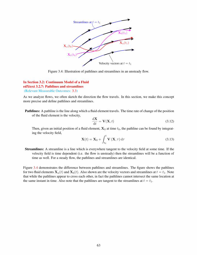
n

Xa(t0)Xa(t1)

Xb(t1)

Xb(t0)

Streamlines at t = t1

Velocity vectors at t = t1

Figure 3.4: Illustration of pathlines and streamlines in an unsteady flow.

In Section 3.2: Continuum Model of a FluidedXtext 3.2.7: Pathlines and streamlines(Relevant Measurable Outcomes: 3.3)

As we analyze flows, we often sketch the direction the flow travels. In this section, we make this conceptmore precise and define pathlines and streamlines.

Pathlines: A pathline is the line along which a fluid element travels. The time rate of change of the positionof the fluid element is the velocity,

dX

dt= V(X, t) (3.12)

Then, given an initial position of a fluid element, X0 at time t0, the pathline can be found by integrat-ing the velocity field,

X(t) = X0 +

∫ t

t0

V (X, τ) dτ (3.13)

Streamlines: A streamline is a line which is everywhere tangent to the velocity field at some time. If thevelocity field is time dependent (i.e. the flow is unsteady) then the streamlines will be a function oftime as well. For a steady flow, the pathlines and streamlines are identical.

Figure 3.4 demonstrates the difference between pathlines and streamlines. The figure shows the pathlinesfor two fluid elements Xa(t) and Xb(t). Also shown are the velocity vectors and streamlines at t = t1. Notethat while the pathlines appear to cross each other, in fact the pathlines cannot intersect the same location atthe same instant in time. Also note that the pathlines are tangent to the streamlines at t = t1.

63

In Section 3.3: Introduction to Control Volume AnalysisedXtext 3.3.1: Control volume definition(Relevant Measurable Outcomes: 3.4)

In developing the equations governing aerodynamics, we will invoke the physical laws of conservation ofmass, momentum, and energy. However, because we are not dealing with isolated point masses, but rathera continuous deformable medium, we will require new conceptual and mathematical techniques to applythese laws correctly.

One concept is the control volume, which is an identified volume of space containing fluid to which we willapply the conservation laws. In principle, the volume could be chosen to move and deform its shape astime evolves. However, in many cases, the control volume is stationary in an appropriately chosen frame ofreference. This type of control volume which is fixed in space is frequently refered to as an Eulerian controlvolume. Figure 3.5 shows an Eulerian control volume. In this example, the flow travels freely through thecontrol volume boundaries. In other situations, a portion of the control volume boundary may correspond toa solid surface (e.g. the surface of a wing) through which flow cannot pass.

Sn

V

(a) Eulerian control volume

Sn

V

(b) Lagrangian control volume

t = t0

t = t1

t = t2

Figure 3.5: Examples of an Eulerian control volume and Lagrangian control volume (i.e. control mass). Ineither case, the volume is denoted V with its boundary surface denoted S and the outward pointing normalat some location on the surface is n.

A closely related concept is the control mass, which is an identified mass of the fluid to which the conserva-tion principles are applied. The control mass though will move with the fluid and deform it shape. In fact,a control mass is equivalent a control volume which is defined to follow the fluid. Often, a control mass isrefered to as a Lagrangian control volume. An example of a Lagrangian control volume (i.e. control mass)is shown in Figure 3.5.

64

In Section 3.3: Introduction to Control Volume AnalysisedXtext 3.3.2: Conservation of mass and momentum(Relevant Measurable Outcomes: 3.4)

Before deriving the mathematical statements of the conservation of mass and momentum applied to Euleriancontrol volumes, we will first state these laws.

Conservation of mass: The conservation of mass requires that mass cannot be created or destroyed. Interms of an Eulerian control volume, mass can enter or leave the control volume at its boundaries. However,since mass cannot be created or destroyed, this means that the mass in the control volume must change toaccount for the flow of mass across its boundaries. Specifically, stating the conservation of mass as a rateequation applied to an Eulerian control volume, we could say,

d

dt(mass in V) = (flow of mass into V) . (3.14)

However, common convention is to combine the terms and state the conservation of mass as,

d

dt(mass in V) + (flow of mass out of V) = 0 (3.15)

If the two terms on the left were not in balance (i.e. their sum was non-zero), then this would mean thatrate of change of mass in the control volume did not equal the flow of mass into the control volume. Inother words, mass would have been created (or destroyed). Thus, the sum of the terms on the left-hand siderepresents the rate at which mass is created within the control volume, and Equation (3.15) states that therate of mass creation is zero within the control volume.

Conservation of momentum: The conservation of momentum states that the rate of change of momentumin a system is equal to the sum of the forces applied to the system. Using the same convention as for theconservation of mass, conservation of momentum applied to an Eulerian control volume gives,

d

dt(momentum in V) + (flow of momentum out of V) =

∑(forces acting on V) (3.16)

As opposed to mass, momentum can be created (or destroyed) in a control volume if the sum of the forceson the control volume is non-zero.

65

In Section 3.3: Introduction to Control Volume AnalysisedXproblem 3.3.1: Release of pressurized air : 0 Points(Relevant Measurable Outcomes: 3.6, 3.8)

x

y

rod

containerV ⇡ 0

Vout

Controlvolume

A container with pressurized air is being held in place by a rod. The container is emitting air at velocity Vout

as shown in the figure. Inside the container, the velocity of the air is negligible (V ≈ 0) which also impliesthat the momentum in the container is negligible. A control volume that is useful for this problem is alsoshown in the figure.

The rate of change of mass inside the container is:



End of edXabox

The rod is acting on the container with a force that, in the x-direction, is:



End of edXabox

Please provide a short explanation for all of your answers.



End of an edXscript



End of edXabox


66

In Section 3.3: Introduction to Control Volume AnalysisedXproblem 3.3.2: Water flow around a spoon : 0 Points(Relevant Measurable Outcomes: 3.6, 3.8)

Now it is time for a little experimental fluid dynamics! In fact, this is an experiment you can do by yourself.All you need is a spoon and a smooth, steady stream of water. To start with, please take a look at thefollowing video which will show you the experimental set-up.


I will move the spoon into the stream and the stream will curve around the spoon. As a result, the spoon willrotate into a new steady position. As shown in Figure 3.6, the new position of the spoon will be either (A)to the left from its initial position when it first contacts the water, or (B) to the right from its initial positionwhen it first contacts the water.

Final position

Initial position

Final position

Initial position

(A) Spoon moves to the left (B) Spoon moves to the right

Figure 3.6: What will the new position of the spoon be?

Before doing the experiment yourself, apply the conservation principles to determine the motion of thespoon. What do you predict will be the motion of the spoon?



End of edXabox

Please provide a short explanation for your answer.



End of an edXscript

67

http://www.youtube.com/watch?v=_QPCIbMZXuI



End of edXabox


68

In Section 3.4: Conservation of MassedXtext 3.4.1: Rate of change of mass inside a control volume(Relevant Measurable Outcomes: 3.5)

In this section, we will express the rate of change of mass inside the control volume mathematically in termsof the fluid states. Since the density is the mass/volume, we may integrate the density throughout the controlvolume to determine the mass in the control volume,

mass in V =

∫∫∫Vρ dV (3.17)

Then, the time rate of change can be found by differentiating with respect to time,

d

dt(mass in V) =

d

dt

∫∫∫VρdV. (3.18)

For a control volume that is fixed in space, the time derivative can also be brought inside the spatial integralto give,

d

dt(mass in V) =

∫∫∫V

∂ρ

∂tdV. (3.19)

69

In Section 3.4: Conservation of MassedXtext 3.4.2: Mass flow leaving a control volume(Relevant Measurable Outcomes: 3.5)

�Vswept V�t

V · n �t

n

dS

Figure 3.7: Volume of fluid, δVswept, that crosses an infinitesimal surface patch dS in time δt. (Note: sideview shown)

Consider an infinitesimal patch of the surface of the fixed, permeable control volume. As shown in Fig-ure 3.7, the patch has area dS, and normal unit vector n. The plane of fluid particles which are on thesurface at time t will move off the surface at time t+ δt, sweeping out an infinitesimal volume given by,

δVswept = V · nδtdS, (3.20)

where V · n is the component of the velocity vector normal to the patch.

The mass of fluid in this swept volume can be found by multiplying by the density to give,

δmswept = ρV · nδtdS. (3.21)

The total mass that flows out of the entire control volume in time δt can then be found by integrating overthe entire surface,

δmtotal = δt

∫∫SρV · ndS (3.22)

where δt is taken outside of the integral since it is a constant.

The time rate at which the mass leaves the control volume, called the mass flow and often given the symbolm, is then

mass flow = m ≡ limδt→0

δmtotal

δt=

∫∫SρV · ndS. (3.23)

Another commonly used quantity is the mass flux and is defined simply as mass flow per area,

mass flux ≡ ρV · n (3.24)

At a solid surface, V · n = 0 since the flow cannot enter the solid. So the portion of a control volume bound-ary at a solid surface does not contribute to the mass flow. This result is frequently used when performingcontrol volume analysis, and is an important consideration when choosing a control volume.

70

In Section 3.4: Conservation of MassedXtext 3.4.3: Conservation of mass in integral form(Relevant Measurable Outcomes: 3.5)

The conservation of mass for a control volume fixed in space as expressed in Equation (3.15) can be writtenmathematically using the results in Equations (3.18) and (3.23),

d

dt

∫∫∫Vρ dV +

∫∫SρV · ndS = 0. (3.25)

Or, alternatively, using Equation (3.19),∫∫∫V

∂ρ

∂tdV +

∫∫SρV · ndS = 0. (3.26)

71

In Section 3.4: Conservation of MassedXtext 3.4.4: Application to channel flow(Relevant Measurable Outcomes: 3.6)

nn

V2

V1V

V · n = 0n

S1

S2

⇢1, p1

⇢2, p2

Figure 3.8: Channel control volume and flow conditions

Now, let’s apply the integral form of conservation of mass to the channel flow shown in Figure 3.8. The flowis assumed to have uniform velocity, density, and pressure at its inlet (V1, ρ1, and p1) and outlet (V2, ρ2, andp2). Further, we will assume that the flow in the channel is steady. As we will derive in the following video,conservation of mass requires that,

ρ1V1S1 = ρ2V2S2 (3.27)

Thus, when there is no unsteadiness, the mass flow leaving the outlet is the same as the mass flow enteringthe inlet. Further, we can re-arrange this expression to show that the mass flux varies inversely with the area,

ρ2V2

ρ1V1=S1

S2(3.28)

Thus, when the area increases (as drawn in this figure), the mass flux decreases (or vice-versa when the areadecreases the mass flux increases). For flows where the density is essentially constant (which would be truefor water or for low Mach number air flows), this can be simplied further to,

V2

V1=S1

S2when ρ = constant (3.29)

Thus, when the area increases, the velocity decreases (and vice-versa).


72

http://www.youtube.com/watch?v=U3IhJw7PcqM

In Section 3.4: Conservation of MassedXproblem 3.4.1: Release of pressurized air (mass conservation) : 0 Points(Relevant Measurable Outcomes: 3.6, 3.2)

Suppose that the density and speed of the air emitted from the container in Problem 3.3.1 is ρout = 1.225kg/m3 and Vout = 10 m/sec, and the container exit has a diameter of 0.2 m.

What is the rate of change of mass in the container in kg/sec?



End of edXabox

Which of the following statements best describes the flow in the container:



End of edXabox


73

In Section 3.5: Conservation of MomentumedXtext 3.5.1: Rate of change of momentum inside a control volume(Relevant Measurable Outcomes: 3.7)

In this section, we will express the rate of change of momentum inside the control volume mathematically interms of the fluid states. This section is an extension of the results in Section 3.4.1. The momentum/volumeis given by ρV, which we may integrate throughout the control volume to determine the momentum in thecontrol volume,

momentum in V =

∫∫∫VρV dV (3.30)

Then, the time rate of change can be found by differentiating with respect to time,

d

dt(momentum in V) =

d

dt

∫∫∫VρV dV. (3.31)

For a control volume that is fixed in space, the time derivative can also be brought inside the spatial integralto give,

d

dt(momentum in V) =

∫∫∫V

∂

∂t(ρV) dV. (3.32)

We can also consider a specific component of the momentum, as opposed to the entire momentum vector.For example, the time rate of change for the j-momentum component in the control volume is,

d

dt(j-momentum in V) =

d

dt

∫∫∫Vρuj dV =

∫∫∫V

∂

∂t(ρuj) dV. (3.33)

74

In Section 3.5: Conservation of MomentumedXtext 3.5.2: Momentum flow leaving a control volume(Relevant Measurable Outcomes: 3.7)

Following the same approach as in Section 3.4.2, the flow of momentum out of the entire control volume

momentum flow =

∫∫SρVV · ndS, (3.34)

and the momentum flux is,momentum flux ≡ ρVV · n (3.35)

Considering only the j-component of momentum gives,

j-momentum flow =

∫∫Sρuj V · ndS, (3.36)

and the j-momentum flux is,j-momentum flux ≡ ρuj V · n (3.37)

As with the mass flow, since at a solid surface, V · n = 0 then the portion of a control volume boundary ata solid surface does not contribute to the momentum flow out of the control volume.

75

In Section 3.5: Conservation of MomentumedXproblem 3.5.1: Release of pressurized air (momentum flow) : 0 Points(Relevant Measurable Outcomes: 3.8)

Consider again the container in Problem 3.4.1. Recall from that problem that ρout = 1.225 kg/m3 andVout = 10 m/sec, and the container exit has a diameter of 0.2 m.

What is the flow of x-momentum out of the container (in units of Newtons)?



End of edXabox


76

In Section 3.5: Conservation of MomentumedXtext 3.5.3: Forces acting on a control volume(Relevant Measurable Outcomes: 3.7)

We will consider two types of forces that act on the control volume:

Body force: a force acting within the volume. In our case, the body force will be gravity.

Surface force: a force acting on the surface of the control volume. In our case, the surface forces arisingfrom the fluid will be due to pressure and viscous stresses. In addition, we will occasionally includesurface forces arising from structures that are cut by the control volume surface.

A common difficulty with this distinction of body and surface forces is that, in fact, the pressure and viscousstresses which give rise to the surfaces forces are present inside the volume. However, within the controlvolume, these forces are balanced between neighboring fluid elements. For example, consider two neigh-boring fluid elements, element A and element B. The pressure force applied by element A on element B isexactly the opposite of the pressure force applied by element B on element A. Thus, the result is no net forcewithin the volume. However, at the surface of the volume, the pressure produces a non-zero force acting onthe fluid that is inside the control volume. The same argument also applies to viscous forces.

The body force due to gravity can be found by integrating the gravitational force/volume over the entirecontrol volume. The gravitational force/volume is given by ρg where g is the gravitational acceleration.Thus, the body force due to gravity acting on the control volume is,

gravitational force on V =

∫∫∫Vρg dV (3.38)

The pressure and viscous force acting on the surface of a control volume can be determine in the samemanner as the pressure and viscous force acting on the surface of the body in Equation (2.7). Thus, thepressure and viscous forces acting on the control volume are,

pressure force on V = −∫∫Sp ndS, (3.39)

viscous force on V =

∫∫Sτ dS, (3.40)

The forces can also be broken into individual components. Doing this give the force in the j-direction as,

j-component of gravitational force on V =

∫∫∫Vρgj dV (3.41)

j-component of pressure force on V = −∫∫Sp nj dS, (3.42)

j-component of viscous force on V =

∫∫Sτj dS, (3.43)

where gj = g · ej , nj = n · ej , and τj = τ · ej and ej is the unit vector in the j-coordinate direction.

Occasionally, we are interested in including forces that act on the control volume that do not arise in thefluid. An example of this situation is in Problem 3.3.1 where the support rod is cut by the control volume.To denote this possibility, we will include

∑Fext to represent external forces applied to the control volume.

Here, we use the word external to represent forces acting on the control volume that are not part of the fluid.When this situation occurs, some region of the control volume must be of non-fluid substance, i.e. there is

77

a region in the control volume that is outside the fluid. Thus, all of the forces which could be included in acontrol volume analysis are, ∫∫∫

Vρg dV −

∫∫Sp ndS +

∫∫Sτ dS +

∑Fext (3.44)

When using a control volume that includes not only the fluid but also other materials, if the mass or mo-mentum of the other materials are changing inside the control volume, then that must be accounted for inthe application of the conservation law. In the equations we develop, we will assume that the only dynamicsoccur in the fluid portions of the control volume.

78

In Section 3.5: Conservation of MomentumedXproblem 3.5.2: Release of pressurized air (forces) : 0 Points(Relevant Measurable Outcomes: 3.8)

Consider again the container in Problem 3.5.1. Recall from that problem that ρout = 1.225 kg/m3 andVout = 10 m/sec, and the container exit has a diameter of 0.2 m.

Further, assume that the air pressure outside of the container (including in the jet emitting from the container)is everywhere equal to the atmospheric pressure, p∞ = 1.01×105 Pascals (Pa). Note that this is a reasonableassumption for a nozzle in which the streamlines enter the atmosphere in parallel, straight lines. If thepressure in the jet were different than p∞, then the streamlines would curve (inward if the pressure in thejet were less than p∞ and outward if the pressure in the jet were greater than p∞). We will investigate thisphenomenon later in the semester.

What is the x-component of the pressure force with which the air acts on the control volume (in units ofNewtons)?



End of edXabox


79

In Section 3.5: Conservation of MomentumedXtext 3.5.4: When are viscous contributions negligible?(Relevant Measurable Outcomes: 3.7)

An important, often subtle, part of control volume analysis is determining when viscous contributions arenegligible on a surface of the control volume. Understanding how to choose a control volume such thatviscous contributions have negligible impact on the analysis is critical.

In the following video, we discuss when viscous contributions are negligible. We then apply this to thepressurized air container of Problem 3.5.2.


80

http://www.youtube.com/watch?v=bG4eS84GySs

In Section 3.5: Conservation of MomentumedXtext 3.5.5: Conservation of momentum in integral form(Relevant Measurable Outcomes: 3.7)

The conservation of momentum for a control volume fixed in space as expressed in Equation (3.16) can bewritten mathematically using the results in Equations (3.31) (3.34), (3.38), (3.39), and (3.40),

d

dt

∫∫∫VρV dV +

∫∫SρVV · ndS =

∫∫∫Vρg dV −

∫∫Sp ndS +

∫∫Sτ dS +

∑Fext. (3.45)

Or, alternatively, using Equation (3.32),∫∫∫V

∂

∂t(ρV) dV +

∫∫SρVV · ndS =

∫∫∫Vρg dV −

∫∫Sp ndS +

∫∫Sτ dS +

∑Fext. (3.46)

Considering only the j-component of momentum gives,∫∫∫V

∂

∂t(ρuj) dV +

∫∫Sρuj V · ndS =

∫∫∫Vρgj dV −

∫∫Sp nj dS +

∫∫Sτj dS +

∑Fextj . (3.47)

For many aerodynamics applications, the gravitational forces are very small compared to pressure and vis-cous forces. Thus, unless we specifically mention to include gravitational forces, we will employ the fol-lowing forms of the momentum conservation equation,∫∫∫

V

∂

∂t(ρV) dV +

∫∫SρVV · ndS = −

∫∫Sp ndS +

∫∫Sτ dS +

∑Fext. (3.48)

or, considering only the j-component of momentum,∫∫∫V

∂

∂t(ρuj) dV +

∫∫Sρuj V · ndS = −

∫∫Sp nj dS +

∫∫Sτj dS +

∑Fextj . (3.49)

81

In Section 3.5: Conservation of MomentumedXproblem 3.5.3: Release of pressurized air (momentum conservation) : 0 Points(Relevant Measurable Outcomes: 3.8)

Consider again the container in Problem 3.5.2. Recall from that problem that ρout = 1.225 kg/m3 andVout = 10 m/sec, and the container exit has a diameter of 0.2 m. Also, the air pressure outside of thecontainer is everywhere equal to the atmospheric pressure, p∞ = 1.01× 105 Pascals (Pa).

What is the x-component of the force that the rod acts with upon the container (in units of Newtons)?



End of edXabox


82

In Section 3.5: Conservation of MomentumedXtext 3.5.6: Application to channel flow(Relevant Measurable Outcomes: 3.8)

Now, let’s apply the integral form of conservation of momentum to the channel flow shown in Figure 3.8.Previously, in Section 3.4.4, we applied the integral form of the conservation of mass. As before, the flowis assumed to have uniform velocity and density at its inlet (V1 and ρ1) and outlet (V2 and ρ2). Further, theflow in the channel is assumed to be steady.

As is described in the following video, applying the x-momentum equations gives,

m (V2 − V1) = p1S1 − p2S2 +

∫∫Swall

p dSx +

∫∫Swall

τ · i dS, (3.50)

where m = ρ1V1S1 = ρ2V2S2 is the mass flow in the channel.

The video discusses an alternative control volume which does not include the boundary layers, and thereforeviscous forces are negligible in this alternative control volume. Using this alternative control volume, weshow that if the boundary layers in the channel are small (compared to the diameter of the channel), thenthe viscous forces can be neglected. The resulting inviscid application of the conservation of x-momentumproduces,

m (V2 − V1) = p1S1 − p2S2 +

∫∫Swall

p dSx. (3.51)


83

http://www.youtube.com/watch?v=SjSnwOmTbIs

In Section 3.6: Sample ProblemsedXproblem 3.6.1: Lift generation and flow turning : 0 Points(Relevant Measurable Outcomes: 2.2, 3.8)

In this example problem, we will apply conservation of y-momentum to relate the lift generated by anairplane (or other body) to the turning of the flow. We will use the control volume shown in Figure 3.9.

x ! �1p = p1

⇢ = ⇢1

V = [V1, 0, 0]

y ! +1, p = p1, ⇢ = ⇢1, V = [V1, 0, 0]

y ! �1, p = p1, ⇢ = ⇢1, V = [V1, 0, 0]

x

y

x = xw

p = pw(y)

⇢ = ⇢w(y)

V = [uw(y), vw(y), ww(y)]

Figure 3.9: Control volume for sample problems.

The lift can be related to an integral of the flow properties in the downstream wake boundary of the form,

L =

∫∫Sw

integrand dS. (3.52)

Determine the integrand required to calculate the lift.


84

In Section 3.6: Sample ProblemsedXproblem 3.6.2: Drag and the wake : 0 Points(Relevant Measurable Outcomes: 2.2, 3.8)

In this example problem, we will now apply conservation of x-momentum to relate the drag generated byan airplane (or other body) to the flow properties in the wake. Again, we will use the control volume shownin Figure 3.9.

The drag can be related to an integral on the downstream wake boundary of the form,

D =

∫∫Sw

integrand dS. (3.53)

Determine the integrand required to calculate the drag.


85

Module 4

Conservation of Energy and Quasi-1D Flow

87


In this module, we consider the conservation of energy as the third of our conservation laws in addition tomass and momentum conservation. Again, we use control volume analysis. We also introduce the adiabaticand isentropic process as a useful model of many compressible aerodynamic flows. Finally, the adiabaticand isentropic flow approximation is combined with a quasi-one-dimensional assumption to derive a usefulmodel for flow through variable area passages, e.g. a converging-diverging nozzle.


4.1 Describe the differences between constant density, incompressible, and compressible flows.

4.2 Relate the pressure, density, and temperature using the ideal gas law. State the definitions of thespecific internal energy and specific enthalpy and relate these to the temperature and specific heats fora calorically perfect gas.

4.3 Explain the physical meaning of the terms of the integral form of energy conservation.

4.4 Apply the integral form of energy conservation to typical problems in aerospace engineering.

4.5 Define the speed of sound for a general compressible flow, derive its relationship to changes in pres-sure and density, and state its dependence on temperature for an ideal gas.

4.6 Define stagnation enthalpy, temperature, pressure, density, etc. and state their relationship to en-thalpy, temperature, pressure, density, etc. and the Mach number for a perfect gas. Derive Bernoulli’sequation from the low Mach number limit of the stagnation pressure relationship.

4.7 Define the assumptions of an adiabatic and isentropic flow and appropriately apply these to calculatevariations in flow properties.

4.8 Derive and apply an isentropic, adiabatic quasi-one-dimensional flow model.

88


The material in this module requires vector calculus and all of the measurable outcomes from Module 3.

89

V

Increasing pressure

Decreasingvolume

Compressible

IncompressibleLagrangiancontrol volume

Figure 4.1: Lagrangian control volume in compressible and incompressible flow

In Section 4.2: Introduction to Compressible FlowsedXtext 4.2.1: Definition and implications(Relevant Measurable Outcomes: 4.1)

A compressible substance is one for which the volume changes when the pressure acting on the materialchanges. This is equivalent to saying that the density of a substance changes with the pressure. Our maininterest is air, and air is compressible. Water (and other liquids more generally) are less compressible thanair (and other gases more generally). Thus, for the same changes in pressure, the density of air will changemore than the density of water.

A compressible flow is a flow in which the fluid density ρ changes with variations in the pressure. Or,somewhat redundantly, a compressible flow is one for which the fluid is compressible! While air flows aretechnically compressible, for many important applications, the changes in density due to pressure variationsare small. In these situations, we can assume the flow is an incompressible flow. While we will discuss thismore throughout this module (and later in the course), density variations tend to be small when the localflow Mach number remains below 0.3 or so. Conversely, for flows with local Mach numbers above 0.3or so, compressibility must be accounted for. The effects become especially large when the Mach numberapproaches and exceeds unity.

Figure 4.1 shows the behavior of a moving Lagrangian Control Volume (CV) which by definition surrounds afixed mass of fluid m. In incompressible flow the density ρ does not change, so the CV’s volume V = m/ρmust remain constant, though its shape can change. In the compressible flow case, the CV is squeezedor expanded in response to pressure changes, with ρ changing in inverse proportion to V . Since the CVfollows the streamlines, changes in the CV’s volume must be accompanied by changes in the streamlinesas well. Compared to incompressible flows, this will mean that the streamlines contract or expand more incompressible flows.

While pressure variations do not change the density of an incompressible substance, an incompressiblesubstance can be heated to produce a density change. Thus, a difference exists between a constant densityflow (in which the density of the fluid is assumed constant) and an incompressible flow (in which the densityof the fluid changes due to temperature variations but not pressure variations). For air flows, heating andcooling through convecting air over a cold or hot surface are common scenarios in which the air flow is oftenwell-approximated as incompressible, though not constant density. While these flows often have quite lowMach numbers, the density variations of the air can be non-negligible because of the heat transfer.

90

In Section 4.2: Introduction to Compressible FlowsedXtext 4.2.2: Ideal gas equation of state(Relevant Measurable Outcomes: 4.2)

An ideal gas is one whose individual molecules interact only via direct collisions, with no other intermolec-ular forces present. For such an ideal gas, the properties p, ρ, and the temperature T are related by thefollowing equation of state,

p = ρRT (4.1)

where R is the specific gas constant which for air, R = 287 J/kg-K. In general, the temperature is a time-varying scalar field since p and ρ are also generally time-varying scalar fields.

The appearance of the temperature in the equation of state means that thermodynamics will need to beaddressed. So in addition to the conservation of mass and momentum, we will now also need to considerthe conservation of energy.

91

= +

vi ciV

Figure 4.2: Decomposition of molecular velocity vi into mean (V) and random (ci) motion.

In Section 4.2: Introduction to Compressible FlowsedXtext 4.2.3: Internal energy of a gas(Relevant Measurable Outcomes: 4.2)

The law of conservation of energy involves the concept of internal energy of a system; that is, all of theenergy inside the system. In our case, the system is the fluid in the control volume and the internal energyis the sum of the energies of all the molecules in the control volume. In thermodynamics, the energy isdivided into kinetic energy (associated with the motion of the molecules including velocities, rotations, andvibrations) and potential energy (associated with the static rest energy, chemical bond energy, etc). Whilewe can track all of these energies, in many fluid mechanics applications, only some of these energies change.For example, unless chemical reactions are occurring, the chemical bond energy will not be altered. So, ifa type of energy is known not to change in the flow, then that energy does not need to be explicitly trackedsince it will automatically be conserved.

In this course, we will only consider the kinetic energy of the molecules. First, consider only the kineticenergy due to the translational motion of the molecules (not include rotational and vibrational motions).In a small region, we can decompose the velocity of any given molecule into the average velocity of themolecules in that region and a random contribution as shown in Figure 4.2. The average molecular velocityis the equivalent of our continuum flow velocity as defined in Section 3.2.5. So, the velocity of molecule iis then,

vi = V + ci. (4.2)

Then, we can sum the kinetic energy (due to translation) over all molecules to find the total kinetic energy(due to translation) of the region. Specifically, let M be the molecular mass (i.e. the mass of a singlemolecule), then

Translational energy in region =∑i

1

2Mvi · vi (4.3)

=1

2M∑i

(V ·V + 2V · ci + ci · ci) (4.4)

=1

2NM

(V 2 + c2

)+MV ·

∑i

ci (4.5)

where N is the number of molecules in the region and c2 is the mean of the square of the random velocityin the region,

c2 ≡ 1

N

∑i

ci · ci. (4.6)

Since ci is the variation of the velocity about the mean velocity, then∑

i ci =∑

i(vi −V) = 0. Thus, thetotal translational energy of the molecules in the region is,

Translational energy in region =1

2NM

(V 2 + c2

)(4.7)

92

Dividing by the volume of the region, NM/V is the density so that,

Translational energy in region/Volume =1

2ρ(V 2 + c2

). (4.8)

Returning to our continuum fluid model, we define the specific total energy, e0, as the energy per unit massof the fluid. As with our other flow quantities, this is a time-varying scalar field, e0(x, y, z, t). We thendefine e0 as,

e0 ≡ e+1

2V 2 (4.9)

where e is known as the specific internal energy. Multiplying Equation (4.9) by the density (producing thetotal energy per unit volume for our continuum flow model) and comparing to Equation (4.8) shows that eaccounts for energy due to the random molecular motions. Generally, e will include not only the energy dueto random transitional motion (i.e. 1

2c2) but also energy due to molecular rotations and vibrations. We will

discuss in the Section 4.2.4 how we model e for air.

With this definition of the specific total energy, the energy inside a control volume is then,

E =

∫∫∫Vρ e0 dV. (4.10)

93

In Section 4.2: Introduction to Compressible FlowsedXtext 4.2.4: Enthalpy, specific heats, and perfect gas relationships(Relevant Measurable Outcomes: 4.2)

Enthalpy

In addition to the specific internal energy e, a related and often-used quantity is the specific enthalpy, denotedby h, and related to the other variables by

h ≡ e+ p/ρ (4.11)

Note that the units of e and h are (velocity)2, or m2/s2 in SI units.

Analogous to the specific total energy, we also define the specific total enthalpy as,

h0 ≡ h+1

2V 2 = e+

p

ρ+

1

2V 2 = e0 +

p

ρ. (4.12)

As we will show in the derivation of the conservation of energy in Section 4.3.4, the enthalpy incorporatesthe pressure work term, and, of key importance in aerodynamics, the total enthalpy is often a constant inmany parts of a flow (see Section 4.3.5).

Thermodynamic equilibrium

We will assume that the gas (i.e. air) is in thermodynamic equilibrium. Thermodynamic equilibrium requiresthe system (i.e. the gas) to be in balance such that there are no unbalanced forces (mechanical equilibrium),no temperature differences (thermal equilibrium), and no chemical reactions (chemical equilibrium).

Thermodynamic equilibrium is not strictly achieved by many fluid flows that are undergoing an unsteadymotion (since unsteady flows are frequently driven by a lack of balanced forces or temperatures, or chemicalreactions occurring). Thermodynamic equilibrium is still a good approximation for a gas if molecular colli-sions occur much more rapidly than any processes that are causing change in the gas. Since air at conditionsof interest to us can have on the order of 1010 collisions per second, thermodynamic equilibrium is often areasonable approximation.

When a gas is in thermodynamic equilibrium, any thermodynamic property can be determined from twoother thermodynamic properties. This means for example that we can think of e as a function e(T, p) ore(T, ρ) or e(p, ρ) or any other pair of properties.

Specific heats

Two very useful quantities are the specific heats at constant volume and constant pressure which are definedas,

cv ≡∂e

∂T

∣∣∣∣v

,

cp ≡∂h

∂T

∣∣∣∣p

.

v is called the specific volume and is defined as v = 1/ρ. Hence, cv is the derivative of e with respectto T holding the specific volume fixed. Similarly, cp is the derivative of h with respect to T holding thepressure fixed. While the specific heats have been defined mathematically as the partial derivatives, theyhave a physical meaning which is hinted at by the specific heat term. Consider a system at some uniformstate. The amount of heat addition required to raise the temperature of the state when the volume of thesystem is held fixed can be shown to be cv∆T (per unit mass, hence specific). Similarly, the heat additionrequired to raise the temperature of the system if the pressure is held fixed can be shown to be cp∆T (perunit mass again).

Thermally perfect gas

94

For a thermally perfect gas, the internal energy is assumed to be only a function of temperature, e = e(T ).This implies from Equations (4.11) and (4.1) that the enthalpy is also only a function of temperature, h =h(T ). Further, since

h − e = p/ρ = RT, (4.13)

we can differentiate this with respect to T to produce,

dh

dT− de

dT= R. (4.14)

Therefore, we see that for a thermally perfect gas,

cp − cv = R (4.15)

Defining the ratio of specific heats, γ ≡ cp/cv, we can with a bit of algebra write

cv =1

γ − 1R

cp =γ

γ − 1R

so that cv and cp can be replaced with the equivalent variables γ and R.

Calorically perfect gas

Restricting our gas model further to a calorically perfect gas, then cv and cp are assumed to be constant.This is an excellent model for air at moderate temperatures (say from -50◦ to 1000◦ C) and we will use itthrough this course. For air, γ = 1.4 is a good approximation (even at 1000◦ C this is within about 6% ofthe actual value of 1.321). Also, it is handy to remember,

γ = 1.4,1

γ − 1= 2.5,

γ

γ − 1= 3.5 (4.16)

such that cv = 717.5 J/kg-K and cp = 1005 J/kg-K.

For a calorically perfect gas, e and h have the simple linear relationships with T ,

e = cv T (4.17)

h = cp T (4.18)

95

In Section 4.2: Introduction to Compressible FlowsedXproblem 4.2.1: Comparing air and battery energy : 0 Points(Relevant Measurable Outcomes: 4.2)

We often teach aerodynamics in Room 33-419 on the MIT campus. This room has a floor area of approx-imately 90 square meters and the ceiling is about 3 meters high. A typical 9-volt battery holds about 19kiloJoules (kJ) of energy. Approximately how many 9-volt batteries are equivalent to the amount of internalenergy of the air in Room 33-419? Note: you only need to account only for the internal energy due to themotion of the air molecules (i.e. no bonding energy, etc.)



End of edXabox


96

In Section 4.3: Conservation of EnergyedXtext 4.3.1: Introduction to conservation of energy(Relevant Measurable Outcomes: 4.3)

The first law of thermodynamics, which we will refer to as the conservation of energy, applied to our Euleriancontrol volume is,

d

dt(energy in V) + (flow of energy out of V) = (rate of work done on V) + (rate of heat added to V)

(4.19)

The first two terms are analogous to the terms in the conservation of mass and momentum. For energy, theseterms take the mathematical form,

d

dt(energy in V) =

d

dt

∫∫∫Vρe0 dV =

∫∫∫V

∂

∂t(ρe0) dV. (4.20)

energy flow =

∫∫Sρe0 V · ndS. (4.21)

97

In Section 4.3: Conservation of EnergyedXtext 4.3.2: Work(Relevant Measurable Outcomes: 4.3)

Work is done on a system as a result of a force being applied in the direction of motion. As we haveexpressed the conservation of energy as a rate equation, we are interested in the rate at which work is doneon the system (i.e. our control volume). Thus, the rate of work done on the control volume can be genericallywritten as F ·V where F is the force applied to a portion of the control volume that is moving with velocityV. The forces we have considered in our fluid dynamics control volume analysis are the pressure, viscous,and external force as given in Equation (3.44). Thus, there are four work terms (note: technically we shouldsay rate of work terms, but we will simply refer to these as work terms with the understanding that they arerates). Specifically, the gravitational work is,

gravitational work =

∫∫∫Vρg ·V dV. (4.22)

The pressure work (also commonly refered to as the flow work) is,

pressure work = −∫∫Sp n ·V dS. (4.23)

The viscous work is,

viscous work =

∫∫Sτ ·V dS. (4.24)

And, the work due to an external force is,

external work =∑

(Fext ·Vext) (4.25)

where Vext is the velocity of the location where the external force is applied.

98

TcoldThot Tfinal

V = 0, p = constant V = 0, p = constant

Figure 4.3: Molecular motion in regions with an initial temperature difference. Even without any bulkmotion, energy will be exchanged between these regions such that the temperatures will eventually equalize.

In Section 4.3: Conservation of EnergyedXtext 4.3.3: Heat(Relevant Measurable Outcomes: 4.3)

Energy can also be transferred to a system even without work i.e. without the application of a force duringbulk motion. This energy exchange occurs due to molecular interactions in regions of the flow where thetemperature varies in space, as depicted in Figure 4.3. We will discuss how this heat transfer is modeled laterin the semester. For now, we define the heat flux vector, q as a vector indicating the direction and rate ofenergy exchange per unit area, such that the rate of energy exchange due to heat transfer through the surfaceof the control volume can be found as,

rate of heat added to V = −∫∫Sq · ndS. (4.26)

Note that the negative sign is because the normal is outward pointing, thus q · n is the heat flux out of thecontrol volume.

99

In Section 4.3: Conservation of EnergyedXtext 4.3.4: Conservation of energy in integral form(Relevant Measurable Outcomes: 4.3)

The conservation of energy for a control volume fixed in space as expressed in Equation (4.19) can be writtenmathematically using the results in Equations (4.20), (4.21), (4.22), (4.23), (4.24), (4.25) and (4.26), as∫∫∫

V

∂

∂t(ρe0) dV +

∫∫Sρe0 V · ndS =

∫∫∫Vρg ·V dV −

∫∫Sp n ·V dS +

∫∫Sτ ·V dS(4.27)

+∑

(Fext ·Vext)−∫∫Sq · ndS. (4.28)

When applying conservation of energy, here are a few important observations:

• On a stationary solid wall boundary, the velocity normal to the wall is zero, i.e. V · n = 0. Thus,the pressure work term is zero. Further, when viscous effects are included, the flow velocity mustmatch the wall velocity, which for a stationary wall means the V = 0. That is, not only is the normalcomponent but all components of the flow velocity are zero at a wall assuming viscous effects areincluded. Thus, the viscous work term will also be zero at a stationary wall.

• As with the conservation of momentum, the effects of gravity in the conservation of energy willgenerally be negligible for aerodynamic applications.

• Similar to viscous effects in the momentum equation (see the discussion in Section 3.5.4), heat transferwill generally be small throughout the flow except where boundary layers are present. Further, formany aerodynamic applications, even the flow at a solid wall can be assumed to be adiabatic, meaningthat q · n ≈ 0.

• Often the pressure work term is incorporated into the energy flow term using the specific total enthalpy(h0) such that the conservation of energy becomes,∫∫∫

V

∂

∂t(ρe0) dV +

∫∫Sρh0 V · ndS =

∫∫∫Vρg ·V dV +

∫∫Sτ ·V dS (4.29)

+∑

(Fext ·Vext)−∫∫Sq · ndS. (4.30)

100

In Section 4.3: Conservation of EnergyedXtext 4.3.5: Total enthalpy along a streamline(Relevant Measurable Outcomes: 4.4)

In the video, we apply the conservation of energy to a control volume surrounding a streamline of a steadyflow. We show the important result that the total enthalpy is constant,

h0 = constant in a steady flow (4.31)

along a streamline where the viscous work and heat transfer are negligible.

Another important conclusion on the behavior of total enthalpy is also demonstrated in Sample Prob-lem 4.6.1. In that problem, we move away from a single streamline to consider the entire flow aroundan airfoil. Please make sure to study the analysis here and in that problem carefully.


101

http://www.youtube.com/watch?v=BmaTnwAC69s

In Section 4.4: Adiabatic and Isentropic FlowsedXtext 4.4.1: Entropy and isentropic relationships(Relevant Measurable Outcomes: 4.7)

Entropy is another thermodynamic state property. The entropy is a measure of heat addition and irreversibil-ities (in our case, viscous effects). Entropy is increased by both of these effects. The Gibbs relation canbe used to relate an infinitesimal change in entropy, ds, to changes in other thermodynamic properties,specifically,

Tds ≡ de+ pd(1/ρ) = dh− (1/ρ)dp. (4.32)

The second form in terms of the enthalpy change can be derived from the first using the definition of theenthalpy.

For a thermally perfect gas, the changes in e and h can be expressed in terms of changes in temperature togive (upon dividing through by cvT to clean-up the result a little),

ds/cv ≡dT

T− (γ − 1)

dρ

ρ= γ

dT

T− (γ − 1)

dp

p. (4.33)

An isentropic process is one in which the entropy does not change, i.e. ds = 0. Using Equation (4.33) wecan determine how the changes in the temperature and density are related for such an isentropic process,

dT

T= (γ − 1)

dρ

ρ(4.34)

This result can alternatively be written as,

∂T

∂ρ

∣∣∣∣s

= (γ − 1)T

ρ(4.35)

which indicates the partial derivative is taken with the entropy fixed (i.e. isentropic).

Similar results can also be found for other states and are summarized here,

dT

T= (γ − 1)

dρ

ρ=γ − 1

γ

dp

pfor an isentropic process. (4.36)

Or, alternatively written as partial derivatives,

∂T

∂ρ

∣∣∣∣s

= (γ − 1)T

ρ,

∂T

∂p

∣∣∣∣s

=γ − 1

γ

T

p,

∂p

∂ρ

∣∣∣∣s

= γp

ρ. (4.37)

For a calorically perfect gas, since γ is constant, we may integrate Equation (4.36) to produce,

T2

T1=

(ρ2

ρ1

)γ−1

=

(p2

p1

)(γ−1)/γ

for an isentropic process between 1 and 2. (4.38)

102

In Section 4.4: Adiabatic and Isentropic FlowsedXtext 4.4.2: Speed of sound(Relevant Measurable Outcomes: 4.5)

Sound waves are weak pressure perturbations. The speed, a, at which they propagate is determined byisentropic relationships and can be shown to be,

a2 =∂p

∂ρ

∣∣∣∣s

. (4.39)

From Equation (4.37), the speed of sound for a thermally perfect gas is,

a =

√γp

ρ=√γRT (4.40)

103

In Section 4.4: Adiabatic and Isentropic FlowsedXtext 4.4.3: Stagnation properties(Relevant Measurable Outcomes: 4.6, 4.7)

In Section 4.4.4, we will discuss the analysis of isentropic flows. In this section, we introduce the concept ofa stagnation property which is very useful for the analysis of flows, independent of whether or not the flowsare isentropic.

Suppose at some time and location, the flow state has properties p, ρ, V, T , e, h, etc. We then define astagnation state and stagnation properties as follows:

Stagnation state: the state which would occur when a given flow state is adiabatically and isentropicallydecelerated to zero velocity.

Adiabatic process: A process is one in which no heat is added (or removed) from the system.

Adiabatic and isentropic process: an adiabatic and isentropic must be reversible, meaning that it ispossible for the process to be run in reverse and return to its original state. For a process to bereversible, frictional (i.e. viscous) forces must be zero throughout the system (not just at the systemboundary).

Stagnation properties: the properties of the stagnation state which we will denote as pstag, ρstag, etc.(note that Vstag = 0 of course!)

Stagnation enthalpy: For an adiabatic and isentropic process, the total enthalpy does not change. We haveseen an example of this in the analysis of the flow along a streamline in Section 4.3.5. Specifically,since an adiabatic and isentropic process means no heat transfer and viscous effects occur, then thetotal enthalpy along a streamline will not change. Thus, adiabatic and isentropic deceleration of theflow to stagnation conditions does not change the total enthalpy, i.e.

h0stag = h0 (4.41)

The definition of the total enthalpy gives,

h0stag = hstag +1

2V 2

stag (4.42)

However, since Vstag = 0, then the total enthalpy at stagnation conditions is simply the enthalpy atstagnation conditions, i.e.

h0stag = hstag (4.43)

Combining this result with Equation (4.41) gives that

hstag = h0 (4.44)

We conclude that the stagnation enthalpy of a state is equal to the total enthalpy of that state.

Stagnation temperature: The temperature at the stagnation state can be determined from Equation (4.44)for a calorically perfect gas using h = cpT to give:

hstag = h0 (4.45)

= h+1

2V 2 (4.46)

cpTstag = cpT +1

2V 2 (4.47)

⇒ Tstag = T +1

2

V 2

cp(4.48)

104

With a little additional manipulation, the stagnation temperature and static temperature (i.e. T ) canrelated by the Mach number,

Tstag = T

(1 +

1

2

V 2

cpT

)(4.49)

= T

(1 +

γ − 1

2

V 2

γRT

)(4.50)

= T

(1 +

γ − 1

2

V 2

a2

)(4.51)

⇒ Tstag = T

(1 +

γ − 1

2M2

)(4.52)

Stagnation pressure: The stagnation pressure pstag can be related to the static pressure p from the isen-tropic relationships in Equation (4.38). This is possible because our imagined deceleration is isen-tropic. Thus,

pstag = p

(Tstag

T

) γγ−1

(4.53)

⇒ pstag = p

(1 +

γ − 1

2M2

) γγ−1

(4.54)

Stagnation density: The stagnation density ρstag can be related to the (static) density ρ again using theisentropic relationships in Equation (4.38),

ρstag = ρ

(1 +

γ − 1

2M2

) 1γ−1

(4.55)

Stagnation speed of sound: One last stagnation quantity which is frequently useful is the stagnation speedof sound, astag which can be found by multiplying Equation (4.48) or Equation (4.52) by γR resultingin,

a2stag = a2 +

γ − 1

2V 2 (4.56)

a2stag = a2

(1 +

γ − 1

2M2

)(4.57)

Total versus stagnation properties: For aerodynamic applications, since the total enthalpy and stagnationenthalpy are the same, the terms total and stagnation are used interchangeably. Similarly, we will usethe stagnation and total subscripts interchangeably. For example, p0 and pstag will refer to the samequantity. However, for applications where other forms of energy are included, then the total quantitieswill be generally different from the stagnation quantities.

105

In Section 4.4: Adiabatic and Isentropic FlowsedXproblem 4.4.1: Isentropic variations with local Mach number : 0 Points(Relevant Measurable Outcomes: 4.6)

Identify which lines in the plot correspond to T/Tstag, p/pstag, and ρ/ρstag by dragging the labels to theappropriate place in the legend.



End of edXabox


106

In Section 4.4: Adiabatic and Isentropic FlowsedXtext 4.4.4: Adiabatic and isentropic flow assumptions(Relevant Measurable Outcomes: 4.6, 4.7)

Since many regions in aerodynamic flows have negligible heating and viscous effects, the entropy of a fluidelement does not change throughout much of the flow. The main locations where entropy changes occurare in boundary layers, wakes, and shock waves. Also, the main regions where heat transfer is significant isnear a solid surface. Thus, if these regions are small, aerodynamic flows can often be modeled as adiabaticand isentropic.

Some care is needed though in assuming an adiabatic and isentropic flow depending on what is being es-timated. For example, when estimating the amount of heat transfer that occurs from the air to the body,assuming an adiabatic flow would not be appropriate (that is pretty obvious I suppose). A little more subtly,when estimating the drag, assuming an isentropic flow is not appropriate since this requires viscous effectsto be neglected (hence no drag due to friction will be estimated).

In steady aerodynamic applications , since far upstream of the body the flow tends to be uniform (i.e.V∞, p∞, T∞, etc. are constant), then the upstream stagnation quantities will also be the uniform (andequal to pstag∞, Tstag∞, etc.). Thus, assuming an adiabatic, isentropic steady flow coupled with a uni-form freestream condition implies that the stagnation properties are constant everywhere in the flow. If theupstream flow were non-uniform, then the stagnation properties would generally vary from streamline-to-streamline, though they would be constant along streamlines (in an adiabatic and isentropic steady flow).

107

In Section 4.4: Adiabatic and Isentropic FlowsedXproblem 4.4.2: Density variations in a low Mach number flow around an airfoil : 0 Points(Relevant Measurable Outcomes: 4.4)

M1 = 0.3

M = 0

Mmax = 0.5

Consider the steady air flow around an airfoil in which the freestream Mach number is M∞ = 0.3 andγ = 1.4. Assume the flow can be approximated as adiabatic and isentropic. Suppose the highest local Machnumber of the flow is M = 0.5. The lowest local Mach number will be zero, since the flow will come torest on the airfoil (even in the isentropic flow where viscous effects are neglected, there is a stagnation pointon the body, in the vicinity of the leading-edge of the airfoil).

What is the ratio of the maximum density in the flow relative to the freestream density (this will be a numbergreater than one)? Use two decimal points so that your answer has the form X.YZ.



End of edXabox

What is the ratio of minimum density in the flow relative to the freestream density (this will be a numberless than one)? Use two decimal points so that your answer has the form X.YZ.



End of edXabox


108

In Section 4.4: Adiabatic and Isentropic FlowsedXtext 4.4.5: Stagnation pressure for incompressible flow and Bernoulli’s equation(Relevant Measurable Outcomes: 4.6, 4.7)

As was demonstrated in Problem 4.4.2, the variation of density in a low Mach number flow can be verysmall. Thus, for low Mach number flows, we will often assume the flow is incompressible.

In the low Mach number limit, the stagnation pressure also takes on a simplified form. To see this, we derivean approximate form of pstag for low M2 taking a Taylor series in terms of M2:

pstag = p

(1 +

γ − 1

2M2

)γ/(γ−1)

(4.58)

pstag ≈ p+ pγ

2M2 +O(M4) (4.59)

Since γpM2 = ρa2M2 = ρV 2, then Equation (4.59) becomes,

pstag ≈ p+1

2ρV 2 (4.60)

Thus, the incompressible definition of the stagnation pressure is recovered in the limit as M2 → 0.

For an adiabatic and isentropic, incompressible (i.e. low Mach number) flow, then we have that,

pstag ≡ p+1

2ρV 2 = constant along a streamline in incompressible flow (4.61)

This is the well-known Bernoulli equation. As in the compressible case, when the flow originates from auniform upstream condition, then p+ 1

2ρV2 is constant everywhere. Later in the course, we will derive the

Bernoulli equation in an alternative manner.

A comment on incompressible flow and the M → 0 limit: We have argued that M → 0 can often beapproximated as an incompressible flow. A common temptation is to think that since M → 0 then V → 0.In other words, the flow is not moving (which would not make for much of a flow)! However, V → 0 is nota requirement of M → 0. An alternative interpretation is to think of the speed of sound as being very largecompared to the flow velocity. Using the definition of the speed of sound in Equation (4.39), an infinitesimalchange in density caused by a infinitesimal change in pressure is:

dρ =1

a2dp (assuming an isentropic perturbation) (4.62)

Thus, a nearly-incompressible substance will have a large speed of sound. Further, the Mach number can bethought of as a non-dimensional measure of the compressibility of the flow.

As an example, consider that the speed of sound of water at room temperature is about 1500 m/s. Bycomparison, air has a speed of sound at room temperature of about 350 m/s. Thus, sound waves travel about4× faster in water than air. Water is much less compressible than air. Further, the flow velocities of interest inwater (i.e. in hydrodynamic applications) are usually much smaller than the flow velocities in aerodynamicapplications. Thus, the Mach number for hydrodynamics will generally be significantly smaller than mostaerodynamic applications, and hydrodynamic applications can be assumed to be incompressible to goodapproximation.

109

V2V1

V · n = 0

S1

S2⇢1, p1

⇢2, p2

V (x)S(x)

⇢(x), p(x)x

y

z

Figure 4.4: Quasi-1D flow model

In Section 4.5: Quasi-1D FlowedXtext 4.5.1: Assumptions

(Relevant Measurable Outcomes: 4.8)

In this section, we utilize the conservation equations and the adiabatic, isentropic relationships to developthe quasi-one-dimensional (quasi-1D) flow model which is depicted in Figure 4.4. The assumptions of thequasi-1D model we will develop in this module are:

• Steady

• Adiabatic

• Isentropic

• Flow properties only depends on x, i.e. ρ(x), p(x), V (x), ...

• The velocity components are negligible in the y and z direction, i.e. |v|, |w| � |u|.

Note that the last two assumptions require that the geometry varies gradually in the x direction.

This quasi-1D flow model has a variety of applications and provides a powerful yet simple method to qual-itatively and often quantitatively estimate the flow behavior. In Section 4.5.2, the incompressible model isdeveloped. Then, the compressible model is developed in Section 4.5.3.

110

p

S S + dS

p + dp

V + dVV

dx

Figure 4.5: Infinitesimal control volume for quasi-1D flow

In Section 4.5: Quasi-1D FlowedXtext 4.5.2: Incompressible quasi-1D flow(Relevant Measurable Outcomes: 4.8)

The conservation of mass for incompressible quasi-1D flow was derived in Section 3.4.4 and given byEquation (3.29), which we write in the following manner,

V S = constant. (4.63)

The Bernoulli equation can then be applied since we have assumed adiabatic, isentropic, and incompressibleflow. Thus we have,

p+1

2ρV 2 = constant. (4.64)

If the cross-sectional area increases, then the velocity decreases (applying conservation of mass) and thepressure increases (applying Bernoulli). And, the opposite trends occur if the area decreases.

While these trends of flow properties with respect to area changes are clear to see for incompressible flow,the corresponding results for compressible flow are more involved. The approach used in compressible flowis to consider infinitesimal changes that occur between x and x + dx. We will apply that analysis here todemonstrate the approach in the simpler incompressible case.

Consider the infinitesimal control volume shown in Figure 4.5. At x and x + dx, we assume that the area,velocity, and pressure are S, V , p and S + dS, V + dV , p + dp, respectively. Then conservation of massgives,

(S + dS)(V + dV ) = SV (4.65)

SV + SdV + V dS + dS dV = SV (4.66)

SdV + V dS + dS dV = 0 (4.67)

SdV + V dS = 0 (4.68)

⇒ dV

V+

dS

S= 0 (4.69)

Note that the fourth step uses the result that the quadratic infinitesimal term (dS dV ) will be small comparedto terms which are linear with respect to dS or dV . Thus, Equation (4.69) illustrates the previous conclusionthat increasing the area (i.e. dS > 0) causes the velocity to decrease (i.e. dV < 0).

An alternative derivation of this result is to differentiate Equation (4.63) directly, i.e.,

d (V S = constant)⇒ SdV + V dS = 0. (4.70)

111

Similarly, differentiating the Bernoulli equation gives,

dp+ ρV dV = 0 (4.71)

⇒ dp

ρV 2+

dV

V= 0 (4.72)

Thus, when dV < 0 then dp > 0.

112

In Section 4.5: Quasi-1D FlowedXtext 4.5.3: Compressible quasi-1D flow(Relevant Measurable Outcomes: 4.8)

For the compressible flow case, the conservation of mass is,

ρV S = constant, (4.73)

As demonstrated for the incompressible flow in Section 4.5.2, we will perform the differential change anal-ysis. For conservation of mass, we find that,

dρ

ρ+

dV

V+

dS

S= 0. (4.74)

Next, we will directly consider the momentum equation. We can utilize the result derived for the inviscidchannel flow in Section 3.5.6. Specifically, applying Equation (3.51) to the infinitesimal control volume inFigure 4.5 gives

ρV SdV = pS − (p+ dp)(S + dS) + p dS. (4.75)

Note that the last term is the approximation of the integral∫p dSx retaining only the terms that are linear in

the infinitesimal changes. The right-hand side can be manipulated to give,

ρV SdV = −S dp. (4.76)

where again only the linear terms are retained. Thus we see that the pressure and velocity changes are relatedby,

dp+ ρV dV = 0. (4.77)

For an incompressible flow, this produces the Bernoulli’s equation result. For the compressible flow case,the result is not Bernoulli’s equation since ρ is not constant. Still, Equation (4.77) can be combined withEquation (4.74) to provide significant insight into quasi-one-dimensional compressible flow.

Since we have assumed the flow is isentropic, changes in pressure and density can be related through thespeed of sound, i.e. dp = a2dρ. Substituting this into Equation (4.77) gives,

dρ

ρ= −M2 dV

V(4.78)

This shows that for low Mach number flows, the fractional change in density will be small compared to thefractional change in velocity. For Mach numbers above one (i.e. supersonic flow), the fractional changes indensity are larger than the fractional changes in velocity. Thus, we have a further illustration for why theMach number can be considered as a non-dimensional measure of the compressibility of a flow.

Then, substituting Equation (4.78) into Equation (4.74) gives,

dV

V=

−1

1−M2

dS

S(4.79)

This key result shows that for subsonic flow, the velocity decreases (dV < 0) for increases in area (dS > 0).Thus, subsonic compressible flow behaves qualitatively like the incompressible case (in fact the limit ofM → 0 produces the incompressible result). However, for supersonic flow the area-velocity relationship isthe opposite: increases in area cause increases in the velocity!

Finally, what happens at M = 1? At a location where M = 1, dV would be infinite unless the cross-sectional area is not changing, i.e. dS = 0. This suggests that the only place where M = 1 can occur isa minimum of the area variation. Note that M = 1 cannot occur at a maximum of the area (even thoughdS = 0). To see this, note that upstream of the area maximum, dS > 0. Though not shown here (because

113

0 0.5 1 1.5 20

0.5

1

1.5

2

2.5

3

3.5

4

4.5

5

M

S/S

∗

Figure 4.6: S/S∗ versus M for γ = 1.4

the derivation is a bit tedious), changes in velocity have the same sign as changes in Mach number. Thus, ifthe flow were subsonic upstream of the area maximum, dM < 0. Similarly, if the flow were supersonic inthis region, then dM > 0. In either case, M = 1 cannot occur at the maximum of the area.

This is a key result which we summarize: M = 1 can only occur at a throat (i.e. a minimum in the area)for a steady, adiabatic, isentropic flow. Note however that the inverse statement is not required, that is, theflow at a throat does not have to be M = 1.

The last step of this analysis will be to algebraically relate the variation in the Mach number and area tofacilitate quantitative analysis of quasi-one-dimensional compressible flows. The common way to do this isto non-dimensionalize the various flow properties by the values at M = 1. Define ρ∗, V ∗, a∗, etc. to be thevalues of these quantities when M = 1. Also, to reduce clutter, we will refer to the stagnation quantities asρ0 and a0.

Applying conservation of mass, gives,ρV S = ρ∗V ∗S∗ (4.80)

Note that V ∗ = a∗ since M = 1 by definition of these quantities. Therefore,

S

S∗=ρ∗

ρ

a∗

V=ρ∗

ρ0

ρ0

ρ

a∗

a0

a0

a

a

V(4.81)

Note that,ρ∗

ρ0=

(γ + 1

2

)− 1γ−1

,a∗

a0=

(γ + 1

2

)− 12

(4.82)

. Using this and the previous ρ/ρ0 and a/a0 relationships produces,

S

S∗=

1

M

[2

γ + 1

(1 +

γ − 1

2M2

)] γ+12(γ−1)

(4.83)

Thus, we have a function which relates the area to the Mach number. S/S∗(M) is plotted in Figure 4.6.

We highlight a few key points about this relationship:

114

• The minimum area does occur at M = 1.

• When analyzing a particular flow, the actual area does not have to equal S∗. It is just a convenientmanner to non-dimensionalize the results.

• The typical approach for solving a problem is to determine e.g. the Mach number at some locationin the flow based on some combination of mass flow and boundary pressures. From this, one candetermine S∗ based on the Mach number and S at the location. With this, the rest of the flow can bedetermined from the ratio of S/S∗ at any other location.

• For any S/S∗ > 1, there is a subsonic and supersonic Mach number possible. Thus, which Machnumber actually occurs will depend on other factors in the problem being analyzed (e.g. upstreamand downstream pressures).

• If a flow was desired to be accelerated from subsonic Mach number to a supersonic Mach number, thearea would first have to contract accelerating the flow to M = 1 at the throat. Then, the area wouldincrease causing the Mach number to increase further if the downstream pressure is sufficiently low tocause further acceleration beyond the throat. Thus, the shape needed to accelerate a flow to supersonicconditions would be a converging-diverging nozzle.

• Another possibility is that a shock wave can occur in the flow. We will discuss this possibility later inthe course.

115

In Section 4.6: Sample ProblemsedXproblem 4.6.1: Total enthalpy in an adiabatic flow : 0 Points(Relevant Measurable Outcomes: 4.4)

In this example problem, we will now apply conservation of energy to the flow around an airplane (orother body). Again, we will use the control volume shown in Figure 3.9. Assume that the airplane body isadiabatic, i.e. q · n = 0 on the body.

Determine the value of the following integral by applying the conservation of energy to the control volume:∫∫Sw

ρwuw (h0w − h0∞) dS =? (4.84)


116

x

y

rod

V ⇡ 0ue

pe = p1p0

T1

SeSt

In Section 4.6: Sample ProblemsedXproblem 4.6.2: Incompressible nozzle flow : 0 Points(Relevant Measurable Outcomes: 4.7, 4.8)

Consider the rocket (in the figure) which is being held in place by the rod (i.e. the test stand). Test standsare used in this manner to estimate the thrust a rocket can generate by measuring the force with which thetest stand must provide to keep the rocket stationary.

The air in the rocket has been compressed to a pressure p0. The temperature of the air in the rocket is theatmospheric temperature T∞. As described in Problem 3.5.2, assuming the streamlines enter the atmospherefrom the nozzle in parallel lines implies that the pressure in the exhaust jet must be equal to p∞. We willconsider this motion in more detail later in the course.

Assume an incompressible, adiabatic, and isentropic flow. You may also assume a steady flow (whichrequires that the flow rate is small so that the impact of the unsteadiness due to the change in mass is small).

Specifically, determine the mass flow m and the force of the rod Frod. How does the throat area St impactm and Frod for incompressible flow?


117

In Section 4.6: Sample ProblemsedXproblem 4.6.3: Subsonic nozzle flow : 0 Points(Relevant Measurable Outcomes: 4.7, 4.8)

Consider again the rocket from Problem 4.6.2. In this problem, we will consider compressibility effects butlimited to subsonic flow (M ≤ 1 everywhere). As before, assume an adiabatic, isentropic, and steady flow.

Determine the mass flow m and the force of the rod Frod. How does the throat area St impact m and Frod

for subsonic compressible flow?


118

In Section 4.6: Sample ProblemsedXproblem 4.6.4: Supersonic nozzle flow : 0 Points(Relevant Measurable Outcomes: 4.7, 4.8)

Consider again the rocket from Problems 4.6.2 and 4.6.3. In this problem, we will consider the supersonicexit flow case. As before, assume an adiabatic, isentropic, and steady flow.

Determine the mass flow m and the force of the rod Frod. How does the throat area St impact m and Frod

for supersonic compressible flow?


119

modules16101x current

Documents

mass flow

conservation of mass

momentum conservation

conservation of momentum

control volume definition

aircraft performance

control volume743

parabolic drag model