module 5: schlieren and shadowgraph lecture 26...

Objectives_template

file:///G|/optical_measurement/lecture26/26_1.htm[5/7/2012 12:34:01 PM]

Module 5: Schlieren and Shadowgraph Lecture 26: Introduction to schlieren and shadowgraph

The Lecture Contains:

Introduction

Laser Schlieren

Window Correction

Shadowgraph

ShadowgraphGoverning Equation and ApproximationNumerical Solution of the Poisson EquationRay tracing through the KDP solution: Importance of the higher-order effectsCorrection Factor for Refraction at the glass-air interfaceMethodology for determining the supersaturation at each stage of the Experiment

Objectives_template



Introduction

Closely related to the method of interferometry are and that employvariation in refractive index with density (and hence, temperature and concentration) to map athermal or a species concentration field. With some changes, the flow field can itself be mapped.While image formation in interferometry is based on changes in the the refractive index withrespect to a reference domain, schlieren uses the transverse derivative for image formation. Inshadowgraph, effectively the second derivative (and in effect the Laplacian ) is utilized.These two methods use only a single beam of light. They find applications in combustion problemsand high-speed flows involving shocks where the gradients in the refractive index are large. Theschlieren method relies on beam refraction towards zones of higher refractive index. Theshadowgraph method uses the change in light intensity due to beam expansion to describe thethermal/concentration field.

Before describing the two methods in further detail, a comparison of interferometry (I), schlieren (Sch)and shadowgraph (Sgh) is first presented. The basis of this comparison will become clear whenfurther details of the measurement procedures are described.

1. Interferometry relies on the changes in the refractive index in the physical region and hencethe changes in the optical path length relative to a known (reference) region. Schlierenmeasures the small angle of deflection of the light beam as it emerges from the test section.Shadowgraph measures deflection as well as displacement of the light beam at the exit planeof the apparatus.

2. Displacement effects of the light beam are neglected in schlieren while displacement as well asdeflection effects are neglected in interferometry. In effect, the light rays are taken to travelstraight during interferometry.

3. Since large gradients will displace and deflect the light beams, interferometry is suitable forsmall gradients and shadowgraph for very large gradients. Schlieren fits well in theintermediate range.

4. In a broad sense, interferometry yields the refractive index field , schlieren - thegradient field and shadowgraph .

5. Since deflection and displacement calculations are more complicated than that of the opticalpath length, shadowgraph analysis is the most involved, schlieren is less so, andinterferometry is the simplest of the three.

6. All the three methods yield a cumulative information of the refractive index field (or itsgradients), integrated in the viewing direction, i.e. along the path of the light beam.

7. As will be seen in the text of this module, schlieren and shadowgraph methods require simpleroptics than interferometry. Shadowgraph is the simplest of all. The price to be paid is in termsof the level (and complexity) of analysis.

Objectives_template



Figure 5.1: A schematic drawing of the schlieren set-up.

A schematic drawing of the schlieren layout is shown in Figure 5.1. In the arrangement shown, lens produces a parallel beam that passes through the test cell TC. Density gradients arising from

temperature gradients in the test cell lead to beam deflection shown by dashed lines 1 and 2 in thefigure above. A discussion on this subject is available in the context of refraction errors ininterferometry.

A key element in the schlieren arrangement is the knife edge. It is an opaque sheet with a sharpedge. The deflected light beam emerging from the test cell is decollimated using a lens or a concavemirror. If the light spot moves downwards, it is blocked by the knife edge and the screen is darkened.If the light spot moves up, a greater quantity of light falls on the screen and is suitably illuminated.Thus, the knife edge serves as a cut-off filter for intensity. An appropriate term that characterizes thisprocess is called contrast, measured as the ratio of change in intensity at a point and the initialintensity prevailing at that location. The knife edge can be seen as an element that controls contrastin light intensity. The change in contrast depends on the initial blockage and hence the initial intensitydistribution on the screen. If the initial (undeflected) light beam is completely cut-off by the knife edge,the screen would be dark. Any subsequent beam deflection would illuminate the screen, thusproducing a significant increase in contrast.

In Figure 5.1, the knife edge is kept at the focus of the lens and the screen at the conjugate focusof the test cell. In other words, the distances satisfy the relation

In Figure 5.1, ray 1 increases the illumination at a point on the screen while ray 2 is blocked by theknife edge and this results in a reduction in the illumination. Hence the image of the scaler field isseen as a distribution of intensities on the screen.

Objectives_template



In a schlieren measurement, beam displacement normal to the knife edge will translate into anintensity variation on the screen. Displacements that are blocked by the knife edge sheet are notrecorded. Similarly, displacements parallel to the knife edge will also not change the intensitydistribution. Information about these gradients in the respective directions can be retrieved by suitablyorienting the knife edge. Other strategies such as using a gray scale filter are available. A color filterleading to a color schlieren measurement is desrcibed later in this module.

Consider the displacement of ray 1 as in Figure 5.2. At point P the illumination is proportional to a,say, equal to . With the test cell in place this becomes . Hence at the contrastwith respect to the undisturbed region is proportional to . The contrast increases greatly whenthe initial illumination is small, but it can lead to difficulties in recording the schlieren pattern. It canbe shown that

and the contrast can be adjusted using the focal length of lens .

Figure 5.2: Initial and final positions of the light spot with respect the knifeedge.

Objectives_template



Laser Schlieren

Image formation in a schlieren system is due to the deflection of light beam in a variable refractiveindex field towards regions that have a higher refractive index. In order to recover quantitativeinformation from a schlieren image, one has to determine the cumulative angle of refraction of thelight beam emerging from the test cell as a function of position in the plane. This plane isdefined to be normal to the light beam, whose direction of propagation is along the coordinate.Thepath of the light beam in a medium whose index of refraction varies in the vertical direction canbe analyzed using the principles of geometric or rays optics as follows:

Consider two wave fronts at times and as shown in Figure 5.3. At time the ray is at aposition . After a interval , the light has moved a distance of times the velocity of light, whichin general, is a function of , and the wave front or light beam has turned an angle . The localvalue of the speed of light is where is the velocity of light in vaccum and is the refractiveindex of the medium. Hence the distance that the light beam travels during time interval is

There is a gradient in the refractive index along the direction. The gradient in results in a bendingthe wave front due to refraction. The distance is given by

Let represent the blending angle at a fixed location . For a small increment in the angle, canbe expressed as

In the limiting case

(1)

Hence the cumulative angle of the light beam at the exit of the test region will be given by

(2)

where the integration is performed over the entire length of the test region.

Objectives_template



If the refrective index within the test section is different from that of the ambient air , then fromSnell's law, the angle of the light beam after it has passed through the test section and emergedinto the surrounding air is given by

For small values of ,

Therefore, Equation 2 gives

If the factor within the integrand does not change greatly through the test section, then

Let be the length of the test section along the direction of the propogation of the light beam. Since the cumulative angle of refraction of the light beam emerging into the surrounding air is

given by

(3)

A schlieren system is basically a device to measure the angle , typically of the order of rad, as a function of position in the x-y plane normal to the light beam. Consider the

system shown in Figure 5.3. A light source with dimensions is kept at the focus of lens and provides a parrallel beam of light which probes the test section.

Figure 5.3: Schematic showing the path of light beam in a typical schlierensystem

Objectives_template


The dotted lines shows the path of the light beam in the presence of disturbances in the test region.The second lens , kept at the focus of the knife-edge collects the light beam and passes onto thescreen located at the conjugate focus of the test section.

Objectives_template



Figure 5.4: View of deflected and undistributed beams at the knife-edge of aschlieren system.

If no disturbance is present, the light beam at the focus of would be ideally as shown in Figure 5.4,with dimensions . These are related to the initial dimensions by the formulas

where and are the focal lengths of and , respectively.

In a schlieren system, the knife edge kept at the focal length of the second concave mirror is firstadjusted, when no disturbance in the test region is present, to cut off all but an amountcorrenponding to the dimension of the light beam Let be the original size of the laser beam.Ifthe knife edge is properly positioned, the illumination at the screen uniformaly changes dependingupon its direction of the movement. Let be the be the illumination at the screen when no knife-edge is present. The illumination with the knife-edge inserted in the focal plane of the of thesecond concave mirror but without any disturbance in the test region will be given by

(4)

Let be the deflection of the light beam in the vertical direction above the knife edgecorresponding to the angular deflection ( ) of the beam after the test region experiences a changein the refractive index. Then from Figure 5.4, can be expressed as

(5)

where the sign is determined by the direction of the displacement of the laser beam in the verticaldirection; it is positive when the shift is in the upward direction and negative if the laser beam gets

Objectives_template


deflected below the level of the knife-edge. In the present discussion, the gradients in the fluid layerare in the upward direction and only the positive sign in Equation 5 is considered.

Objectives_template



Contd...

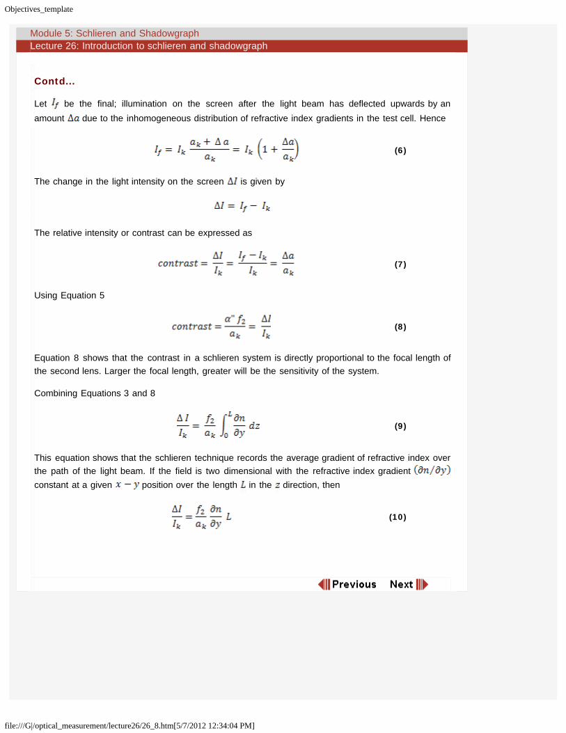
Let be the final; illumination on the screen after the light beam has deflected upwards by anamount due to the inhomogeneous distribution of refractive index gradients in the test cell. Hence

(6)

The change in the light intensity on the screen is given by

The relative intensity or contrast can be expressed as

(7)

Using Equation 5

(8)

Equation 8 shows that the contrast in a schlieren system is directly proportional to the focal length ofthe second lens. Larger the focal length, greater will be the sensitivity of the system.

Combining Equations 3 and 8

(9)

This equation shows that the schlieren technique records the average gradient of refractive index overthe path of the light beam. If the field is two dimensional with the refractive index gradient constant at a given position over the length in the direction, then

(10)

Objectives_template



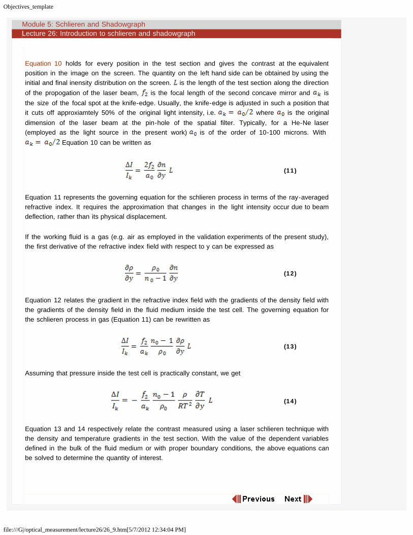
Equation 10 holds for every position in the test section and gives the contrast at the equivalentposition in the image on the screen. The quantity on the left hand side can be obtained by using theinitial and final inensity distribution on the screen. is the length of the test section along the directionof the propogation of the laser beam, is the focal length of the second concave mirror and isthe size of the focal spot at the knife-edge. Usually, the knife-edge is adjusted in such a position thatit cuts off approxiamtely 50% of the original light intensity, i.e. where is the originaldimension of the laser beam at the pin-hole of the spatial filter. Typically, for a He-Ne laser(employed as the light source in the present work) is of the order of 10-100 microns. With

Equation 10 can be written as

(11)

Equation 11 represents the governing equation for the schlieren process in terms of the ray-averagedrefractive index. It requires the approximation that changes in the light intensity occur due to beamdeflection, rather than its physical displacement.

If the working fluid is a gas (e.g. air as employed in the validation experiments of the present study),the first derivative of the refractive index field with respect to y can be expressed as

(12)

Equation 12 relates the gradient in the refractive index field with the gradients of the density field withthe gradients of the density field in the fluid medium inside the test cell. The governing equation forthe schlieren process in gas (Equation 11) can be rewritten as

(13)

Assuming that pressure inside the test cell is practically constant, we get

(14)

Equation 13 and 14 respectively relate the contrast measured using a laser schlieren technique withthe density and temperature gradients in the test section. With the value of the dependent variablesdefined in the bulk of the fluid medium or with proper boundary conditions, the above equations canbe solved to determine the quantity of interest.

Objectives_template



For a growing KDP crystal, the refractive-index field gradients of the KDP solution and theconcentration gradients are related using the following formula:

(15)

Here is the polarizability of the KDP and N is the molarconcentration of the solution (moles per 100 gram of the solution). Combining Equations 9 and 15 andintegrating from a location in the bulk of the solution (where the gradients are negligible) , theconcentration distribution around the growing crystal can be uniquely determined. Equations 13 and14 show that the schlieren measurements are primamarily based on the original intensity distributionas recorded by the CCD camera. Though the schlieren images shown in the present work forqualitative interpretation of the fluids region have been subjected to image processing operations forcontrast enhancement, original images as recorded by the CCD camera are employed for quantitativeanalysis. Figure 5.5 shows a set of four consecutive schlieren images and their averaged image. Theimages show a convective plume in the form of high intensity regions above a crystal growing from itsaqueous solution and are discussed in detail in the subsequent lectures (27-33).

Figure 5.5: Original schlieren images (a-d) of convective field as recorded bythe CCD camera and the corresponding time-averaged image(e).

Objectives_template



Window Correction

For visualization of the concentration field by the schlieren technique, circular optical windows havebeen fixed on the walls of the growth chamber at opposite ends. THe optical window employed in thepresent discussion of crystal growth is of finite thickness (5 mm) and the index of refraction of itsmaterial (BK-7) is considerably different from that of a KDP solution and air. The light beam emergingout of the KDP solution with an angular deflection due to the variable concentration gradients inthe growth chamber again undergoes refraction before finally emerging into the surroundingenvironment. The contribution of refraction of light at the confining optical windows can be accountedfor by applying a correction factor in Equation 11 as discussed below.

The laser beam strikes the second optical window fixed on the growth chamber at an angle afterundergoing refraction due to variable concentration gradients in the vicinity of the growing KDPcrystal. The optical windows are made of BK-7 material with index of refraction equal to1.509. The refractive index of the KDP solution at an average temperature of is equal to1.355 and for air . Let be the angular deflection of the beam purely due to thepresence of concentration gradients in the vicinity of the growing crystal as shown schematically inFigure 5.6.

Figure 5.6: Schematic drawing showing the path of the light beam and thecorresponding angles of deflection as it passes through the growth chamber.

(Dimension in the figure are exaggerated for clarity).

The beam strikes the second optical window at this angle. Let be the angle at which the laserbeam emerges out of the second optical window. The angle at which the laser beam emerges out ofthe second optical window can be determined in terms of using Snell's law as

(16)

Objectives_template



Contd...

Since is quite small, , and

(17)

Let be the final angle of refraction with which the laser beam emerges into the surrounding air. Forthe optical window-air combination,

(18)

Substituting the value of from Equation 17 into Equation 18, the angle with which the laserbeam emerges into the surrounding medium can be expressed as

(19)

or

(20)

Since

(21)

Hence a correction factor equal to the refractive index of the KDP solution at the ambient temperatureis taken into consideration for calculating the angle at which the laser beam emerges into thesurrounding medium.

Objectives_template



Shadowgraph

The shadowgraph arrangement depends on the change in the light intensity arising from beamdisplacement from its original path. When passing through the test field under investigation, theindividual light rays are refracted and bent out of their original path. The rays traversing the regionthat has no gradient are not deflected, whereas the rays traversing the region that has non zerogradients are bent up. Figure 5.7 illustrates the shadowgraph effect using simple geometric raytracing. Here a plane wave traverses a medium that has a nonuniform index of refraction distributionand is allowed to illuminate a screen. The resulting image on the screen consists of regions wherethe rays converege and diverge; these appear as light and dark regions respectively. It is this effectthat gives the technique its name because gradients leave a shadow, or dark region, on the viewingscreen. A particular deflected light ray that arrives at a point different from the original point of therecording plane should be traced. It leads to a distribution of light intensity in that plane altered withrespect to the undistributed case.

When subjected to linear approximations that includes small displacement of the light ray, a secondorder partial differential equation can be derived for the refractive index feild with respect to intensitycontrast in the shadowgraph image. Let D be the distance of the screen from the optical window onthe beaker. The governing equation for a shadowgraph process can be expressed as

(22)

Figure 5.7: Illustration of the shadowgraph arrangement

Objectives_template



Contd...

Here is the change in illumination on the screen due to the beam displacement from its originalpath and is the original intensity distribution. Equation 22 implies that the shadowgraph is sensitiveto changes in the second derivative of the refractive index along the line of sight of the of the lightbeam in the fluid medium. Integration of the Poisson equation (22) can be performed by a numericaltechnique, say the method of finite differences.

From Equation 22 it is evident that the shadowgraph is not a suitable method for quantitativemeasurement of the fluid density, since such an evaluation requires one to perform a doubleintegration of the data. However, owing to its simplicity the shadowgraph is a convenient method forobtaining a quick survey of flow fields with varying fluid density. When the approximations involved inEquation 22 do not apply, shadowgraph can be used for flow visualization alone.

The present lecture has a discussion on how shadowgraph images can be analyzed to retrieveinformation on the concentration field.

Shadowgraphy

It employs an expanded and collimated beam of laser light. The light beam traverses the field ofdisturbance, an aqueous solution of KDP in the present application. If the disturbance is a field ofvarying refractive index, the individual light rays passing through the field are refracted and bent out oftheir original path. This causes a spatial modulation of the light intensity distribution. The resultingpattern is a shadow of the refractive-index field in the region of the disturbance.

Governing equation and Approximations

Consider a medium with refractive index that depends on all the three space coordinates, namely . We are interested in tracing the path of light rays as they pass through this medium.

Starting with the knowledge of the angle and the point of incidence of the ray at the entrance plane,we would like to know the location of the exit point on the exit window, and the curvature of theemergent ray.

Let the ray be incident at point and the exit point be . Accordingto Fermat's principle the optical path length traversed by the light beam between these two points hasto be an extremum. If the geometric path length is , then the optical path length is given by theproduct of the geometric path length with the refractive index of the medium. Thus

(23)

Objectives_template



Parameterizing the light path by , the condition (Equation 23) can be represented by two functions , and the equation can be written as

(24)

where the primes denote differentiation with respect to . Application of the variational principle to theabove equation yields two coupled Euler-Lagrange equations, that can be written in the form of thefollowing differential equations for :

(25)

(26)

The four constants of integration required to solve these equations comes from the boundaryconditions at the entry plane of the chamber. These are the co-ordinates ofthe entry point and the local derivatives . The solution of the aboveequation yields the two orthogonal components of the deflection of the ray at the exit plane, and alsoits gradient on exit.

In the experiments performed, the medium has been confined between parallel planes and theillumination is via a parallel beam perpendicular to the entry plane. The length of the growth chambercontaining the fluid is D and the screen is at a distance behind the growth chamber. The coordinates at entry, exit and on the screen are given by respectively. Since the incidentbeam is normal to the entrance plane, there is no refraction at the optical window. Hence thederivatives of all the incoming light rays at the entry plane are zero; . The displacements

of the light ray on the screen with respect to its entry position are

(27)

(28)

where are given by the solutions of previous equations at .

The above formulation can be further simplified with the following assumptions.

Objectives_template



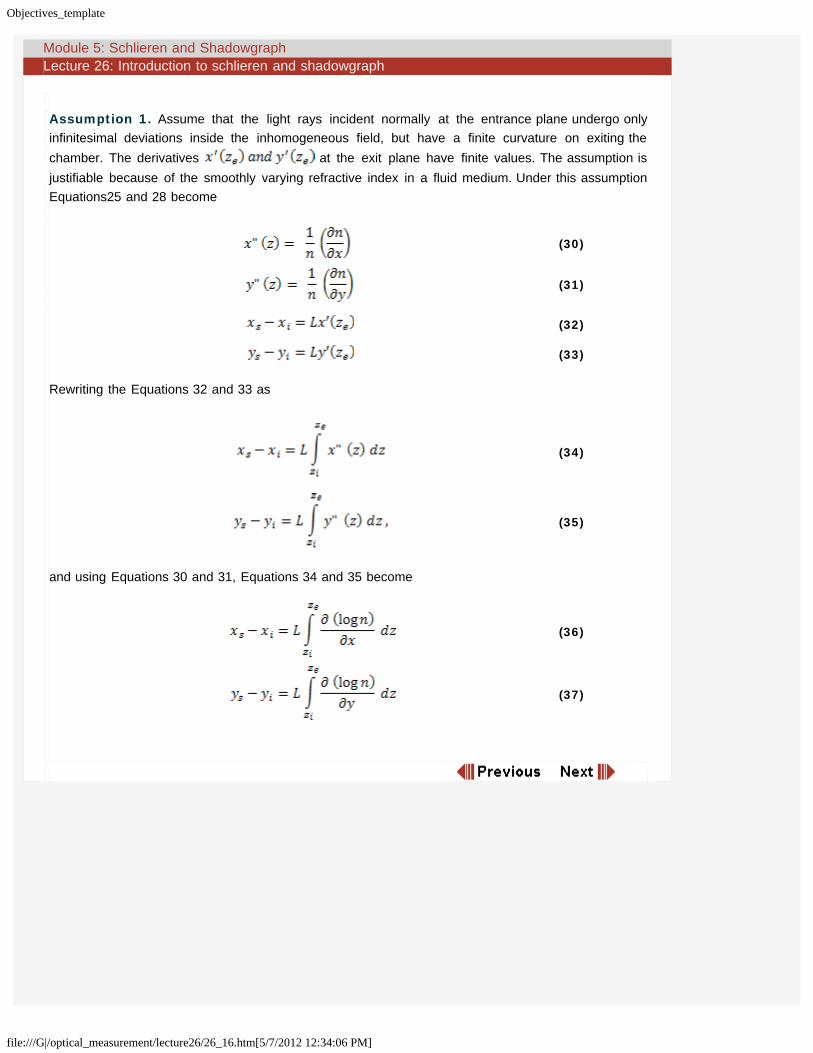
Assumption 1. Assume that the light rays incident normally at the entrance plane undergo onlyinfinitesimal deviations inside the inhomogeneous field, but have a finite curvature on exiting thechamber. The derivatives at the exit plane have finite values. The assumption isjustifiable because of the smoothly varying refractive index in a fluid medium. Under this assumptionEquations25 and 28 become

(30)

(31)

(32)

(33)

Rewriting the Equations 32 and 33 as

(34)

(35)

and using Equations 30 and 31, Equations 34 and 35 become

(36)

(37)

Objectives_template



Assumption 2 : The assumption of the infinitesimal displacement inside the growth chamber can beextended and taken to be valid even for the region falling between the screen and the exit plane ofthe chamber. As a result, the coordinates of the ray on the screen can be written as

(38)

(39)

The deviation of the rays from their original paths in occurs through the inhomogeneous medium. Inthe absence of the inhomogeneous field, such an area is a regular quadrilateral. It transforms to adeformed quadrilateral when imaged on to a screen in the presence of the inhomogeneous field. Thesummation in the above equation extends over all the rays passing through points at theentry of the test section that are mapped onto the small quadrilateral on the screen.Considering the fact that the area of the initial spread of the light beam gets deformed on passingthrough the refractive medium, the intensity at point is

(40)

where is the intensity on the screen in the presence of the inhomogeneous refractive index field,and is the original undisturbed intensity distribution. The denominator in the above equation is theJacobian of the mapping function of onto as shown in Ffigure 5.8.

Figure 5.8: Jacobian of the mapping function onto

Geometrically it represents the ratio of the area enclosed by four adjacent rays after and beforepassing through the inhomogeneous medium. In the absence of the inhomogeneous field, such anarea is a regular quadrilateral. It transforms to a deformed quadrilateral when imaged on to a screenin the presence of the inhomogeneous field. The summation in the above equation extends over allthe rays passing through points at the entry of the test section that are mapped onto thesmall quadrilateral on the screen and contribute to the light intensity within.

Objectives_template



Assumption 3: Under the assumption of infinitesimal displacements, the deflections aresmall. Therefore the Jacobian can be assumed to be linearly dependent on them by neglecting thehigher powers of , and also their product. Therefore, the jacobian can be expressed as

(41)

Substituting in Equation 39, we get

(42)

Simplifying further we get

(43)

Using Equations 36 and 37 for , and integrating over the dimensions of thegrowth chamber, we get

(44)

Equation 44 is the governing equation of the shadowgraph process under the set of linearizingapproximation 1-3. In concise from the above equation can be rewritten as

(45)

Objectives_template



Numerical Solution of the Poisson Equation

The governing equation of the shadowgraph process (Equation 44) relates the intensity variation inthe shadowgraph image to the refractive index field of the inhomogeneous medium. In order to solvethe equation to obtain the refractive index, the following numerical procedure is adopted. First, thePoisson equation is discretized over the physical domain of interest by a finite-difference method. Theresulting system of algebraic equations is solved for the image under consideration to yield a depthaveraged refractive index value for each node point of the grid. A mix of Dirichlet and Neumannboundary conditions are used for the purpose. The refractive index conditions typically used on theboundaries of a crystal growth chamber are shown inn Figure 5.9. A computer code can be written forsolving the Poisson equation, and it can be validated against analytical examples.

Figure 5.9: Refractive index specification on the boundaries.

The experimental input to the code is in the form of a matrix containing the gray value of each pixelof the shadowgraph image. The output generated by the Poisson solver is a matrix containing theaveraged refractive index at each node point of the grid. Since the relationship between theerefractive index and the concentration of the KDP saturated solution at different temperatures is welldocumented, the refractive indices can be related to concentration over every frame of the imagerecord.

Objectives_template



Ray tracing through the fluid medium: Importance of the higher-order effects

In order to assess the importance of higher-order optical effects in shadowgraph imaging, the extentof the bending of rays is estimated by tracing the passage of rays through the fluid phase. In order tobe able to do this, the shadowgraph images of the growth process recorded at different stages ofgrowth are analyzed as follows: The Poisson equation governing the shadowgraph process is solvednumerically to yield a depth-averaged refractive index value for each node point of the grid. Therefractive index information is then used to determine the deflection of the ray at the exit plane of thegrowth chamber by solving the coupled ordinary differential equations (ODEs) governing the passageof light ray through the region of disturbance. The solution of these equation yields the two orthogonalcomponents of the deflection of the ray and its gradient at the exit plane of the test cell. For thePoisson equation to be applicable for shadowgraph analysis, the ray deflections should be small.

Considering the length of the growth chamber containing the fluid as D and the screen to be at adistance behind the test section, the displacements of a light ray on thescreen with respect to its entry position are given by Equations 27 and 28. A computer code forsolving the coupled ODEs has been written and validated against analytical examples.

Correction factor for refraction at the glass-air interface

In order to perform laser shadowgraphic and interferometric imaging of the crystal growth process,two different growth chambers were fabricated. The crystal growth process referred here is describedin detail in lectures 27-33. The growth chambers have optical windows for the entry and exit of thelaser beam. The cavity is enclosed between the windows for the entry and exit of the laser beam.The cavity enclosed between the windows was filled with the KDP solution. During the process ofcrystal growth the KDP solution is a medium of varying refractive index, leading to the bending of therays as the laser beam traverses through the solution. At the exit from the growth chamber, the lightray encounters two different interfaces, namely KDP-solution and glass, followed by glass and air.Thus, the light ray emerges at an angle different from the angle at which it is incident on the solutionand glass interface. The refractive indices of the KDP solution, the quartz window and the air aroundresult in a scale factor which must be taken into account to get the correct emergent angle of ray. Theoptical path of the light ray through the two interfaces is shown in Figure 5.10.

Objectives_template


Figure 5.10: Optical Path of the light ray passing from the growth chamberinto the air.

Objectives_template



(48)

Contd...

The scale factor used in calculations is derived below.

Applying Snell's law for refraction of the light ray passing from the KDP-solution into the quartz opticalwindow, we get

(46)

where are the angles of incidences of the light at the quartz window, theangle of refraction of the light ray into the quartz window, the refractive index of the KDP solution, andthe refractive index of the quartz window respectively. Applying Snell's law again for the ray passingfrom the quartz optical window to the surrounding air, we get

(47)

where are the angles of refraction of the light ray into the quartz window, theangle of refection of the light ray in the air, the refractive index of the quartz window, and therefractive index of air respectively. Substituting the expression for from Equation 46 intoEquation 47, we get

Under the small-angle approximation sin , and

Hence

Thus the correction factor for additional refraction at the optical windows is .

module 5: schlieren and shadowgraph lecture 26...

Documents