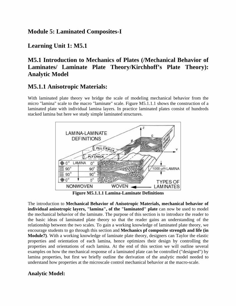
Module 5: Laminated Composites-I Learning Unit 1: M5.1 M5.1 Introduction to Mechanics of Plates (/Mechanical Behavior of Laminates/ Laminate Plate Theory/Kirchhoff’s Plate Theory): Analytic Model M5.1.1 Anisotropic Materials: With laminated plate theory we bridge the scale of modeling mechanical behavior from the micro "lamina" scale to the macro "laminate" scale. Figure M5.1.1.1 shows the construction of a laminated plate with individual lamina layers. In practice laminated plates consist of hundreds stacked lamina but here we study simple laminated structures.

Figure M5.1.1.1 Lamina-Laminate Definitions

The introduction to Mechanical Behavior of Anisotropic Materials, mechanical behavior of individual anisotropic layers, "lamina", of the "laminated" plate can now be used to model the mechanical behavior of the laminate. The purpose of this section is to introduce the reader to the basic ideas of laminated plate theory so that the reader gains an understanding of the relationship between the two scales. To gain a working knowledge of laminated plate theory, we encourage students to go through this section and Mechanics pf composite strength and life (in Module7). With a working knowledge of laminate plate theory, designers can Taylor the elastic properties and orientation of each lamina, hence optimizes their design by controlling the properties and orientations of each lamina. At the end of this section we will outline several examples on how the mechanical response of a laminated plate can be controlled ("designed") by lamina properties, but first we briefly outline the derivation of the analytic model needed to understand how properties at the microscale control mechanical behavior at the macro-scale. Analytic Model:

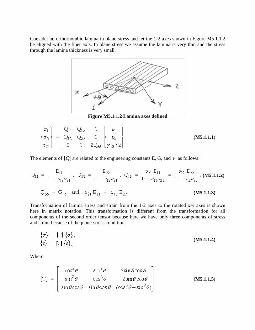
Consider an orthorhombic lamina in plane stress and let the 1-2 axes shown in Figure M5.1.1.2 be aligned with the fiber axis. In plane stress we assume the lamina is very thin and the stress through the lamina thickness is very small.

Figure M5.1.1.2 Lamina axes defined

(M5.1.1.1)

The elements of [ ]Q are related to the engineering constants E, G, and ν as follows:

(M5.1.1.2)

(M5.1.1.3) Transformation of lamina stress and strain from the 1-2 axes to the rotated x-y axes is shown here in matrix notation. This transformation is different from the transformation for all components of the second order tensor because here we have only three components of stress and strain because of the plane-stress condition.

(M5.1.1.4)

Where,

(M5.1.1.5)

The lamina stress-strain relationship in the rotated x-y coordinates,

(M5.1.1.6)

In reduced matrix notation,

(M5.1.1.7) Where,

(M5.1.1.8) The inverse stress-stain relationship relates stresses (known) to strains (unknown) with the compliance,[ ]S matrix,

(M5.1.1.9)

Where,

(M5.1.1.10) Hence there is an inverse relationship between the[ ]S and [ ]Q matrices.

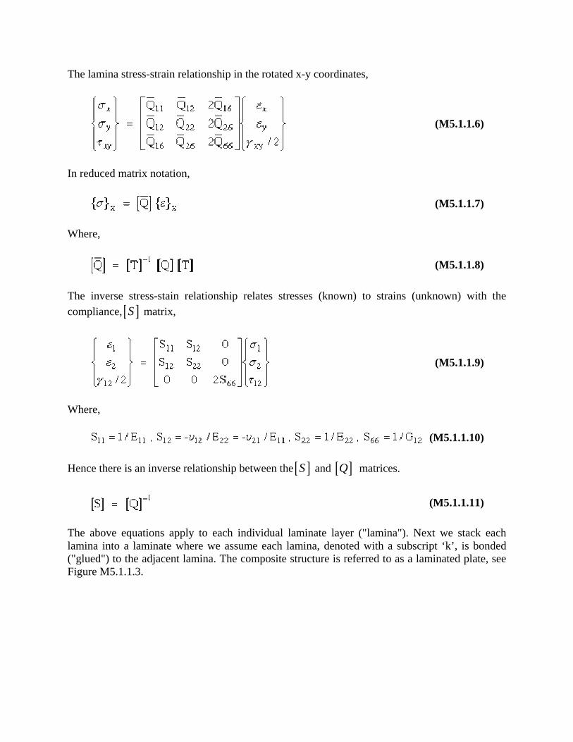
(M5.1.1.11) The above equations apply to each individual laminate layer ("lamina"). Next we stack each lamina into a laminate where we assume each lamina, denoted with a subscript ‘k’, is bonded ("glued") to the adjacent lamina. The composite structure is referred to as a laminated plate, see Figure M5.1.1.3.

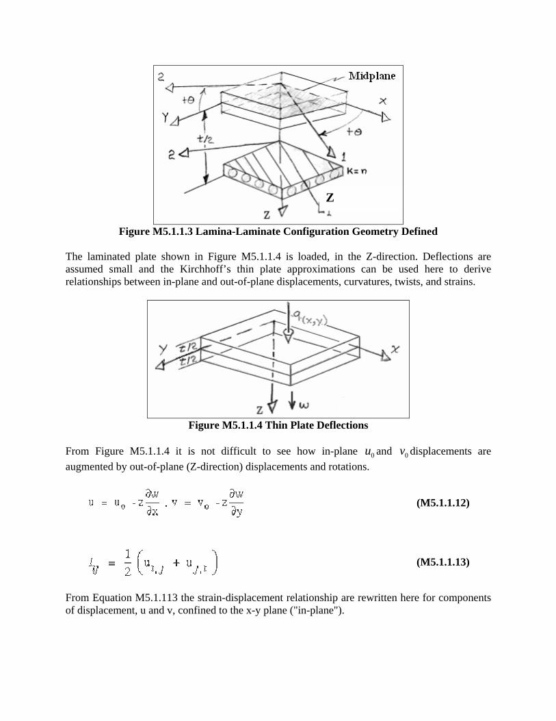
Figure M5.1.1.3 Lamina-Laminate Configuration Geometry Defined

The laminated plate shown in Figure M5.1.1.4 is loaded, in the Z-direction. Deflections are assumed small and the Kirchhoff’s thin plate approximations can be used here to derive relationships between in-plane and out-of-plane displacements, curvatures, twists, and strains.

Figure M5.1.1.4 Thin Plate Deflections

From Figure M5.1.1.4 it is not difficult to see how in-plane 0u and 0v displacements are augmented by out-of-plane (Z-direction) displacements and rotations.

(M5.1.1.12)

(M5.1.1.13)

From Equation M5.1.113 the strain-displacement relationship are rewritten here for components of displacement, u and v, confined to the x-y plane ("in-plane").

Z

(M5.1.1.14)

From the expression of radius of curvature, ρ we derive expressions for curvature, xk and yk assuming small angular deflections.

(M5.1.1.15)

A similar expression for twist ‘ x yk ’ can be derived from Figure M5.1.1.5 where twist is defined as an "angular change" per "unit length".

Figure M5.1.1.5 Exaggerated Thin Plate Deflections and Twists Defined

The coefficient ‘2’ is introduced by convention for engineering shear strain.

(M5.1.1.16)

Combining Equation M5.1.1.15 and Equation M5.1.1.16, into Equation M5.1.1.14 yields

(M5.1.1.17)

Substituting Equation M5.1.1.17 into Equation M5.1.1.16 yields a more general stress-strain relationship for the thk lamina which includes out-of-plane displacement implicitly in the curvature terms.

(M5.1.1.18)

With stresses defined in terms of the Z-coordinate, through the laminate thickness, we integrate these expressions to get the laminate resultant in-plane loads ( x y xyN , N , N ), and moments ( xM ,

y xyM ,M ).

Figure M5.1.1.6 Laminate Plate In-Plane Loads and Moments Defined

(M5.1.1.19)

Substitute Equation M5.1.1.18 into Equation M5.1.1.19 and simplify.

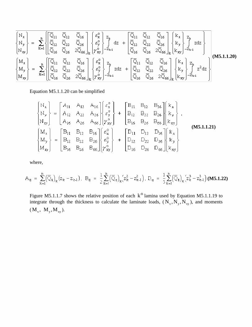
(M5.1.1.20)

Equation M5.1.1.20 can be simplified

(M5.1.1.21)

where,

(M5.1.22)

Figure M5.1.1.7 shows the relative position of each thk lamina used by Equation M5.1.1.19 to integrate through the thickness to calculate the laminate loads, ( x y xyN , N , N ), and moments ( xM , y xyM ,M ).

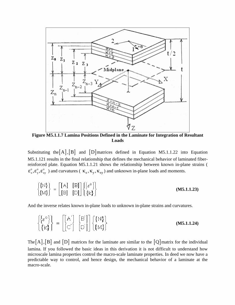
Figure M5.1.1.7 Lamina Positions Defined in the Laminate for Integration of Resultant

Loads Substituting the[ ]A ,[ ]B and [ ]D matrices defined in Equation M5.1.1.22 into Equation M5.1.121 results in the final relationship that defines the mechanical behavior of laminated fiber-reinforced plate. Equation M5.1.1.21 shows the relationship between known in-plane strains (

o o ox y xy, ,ε ε ε ) and curvatures ( x y xy, ,κ κ κ ) and unknown in-plane loads and moments.

(M5.1.1.23)

And the inverse relates known in-plane loads to unknown in-plane strains and curvatures.

(M5.1.1.24)

The[ ]A ,[ ]B and [ ]D matrices for the laminate are similar to the [ ]Q matrix for the individual lamina. If you followed the basic ideas in this derivation it is not difficult to understand how microscale lamina properties control the macro-scale laminate properties. In deed we now have a predictable way to control, and hence design, the mechanical behavior of a laminate at the macro-scale.

Like the lamina at the microscale, anisotropy of the laminate has a significant effect on the mechanical behavior of the laminate. This can best be observed by inspection of Equation M5.1.1.23 and Equation M5.1.1.24. If the individual lamina are stacked and glued together such that the [ ]B matrix is zero then the mechanical behavior exhibits a decoupling of moments and inplane loads. For example curvatures only affect moments and inplane strains only affect inplane load. On the other hand it is not difficult to see that if [ ]B is not zero then there is coupling between curvatures and inplane loads, and coupling also exists between inplane strains and moments. This is rather peculiar. For example if we apply an inplane strain to a specially configured laminate then the laminate can bend more then it would extend ("stretch"). Similarly if we apply an inplane load the laminate will twist. The later is actually used to an advantage by designers of aircraft structures where aircraft wings that are constructed by fiber-reinforced laminates are designed to twist into a predetermined aerodynamic angle-of-attack as the wing bends and extends. This design methodology is called Passive aero-elastic tailoring. With "smart"-"intelligent" structures it is possible to insert active piezoelectric layers into the laminate stacking sequence and Activity control the mechanical behavior of the laminate. The degree of coupling is controlled by the[ ]A ,[ ]B and [ ]D matrices. In this section a few simple examples are presented that illustrate how simple laminate configurations can provide predictable macroscopic mechanical behavior by inspection of Equation M5.1.1.23 and Equation M5.1.1.24. Case I: Symmetric Laminates, [ ]B =0

By inspection when [ ]B is zero, inplane loads and moments decouple in Equation M5.1.1.23 and

Equation M5.1.1.24. Inplane loads { }N only produce inplane strains { }ε and inplane moments

{ }M only produce curvature{ }k . Case II: Specially Orthotropic Symmetric laminates, 16A 0= and 26A 0= Bi-directional laminates consist only of 0 / 9degree lamina. It is not difficult to show 16Q and

26Q are zero. Hence 16A and 26A are also zero and consequently the inplane shear strain

{ }γ decouples from the inplane normal strains. Therefore shearing loads can only produce shearing strains and inplane normal loads can only produce inplane strains Case III: Specially Orthotropic Bending Behavior, 16 26& 0D D → , Number of Lamina→Large For a large number of symmetric pairs, +θ at h+ and −θ at h− , 16D and 26D go to zero. Hence

moments { }xM & { }yM and torque { }xyM decouple so that bending caused by moments do not

introduce twisting and torque that causes twisting does not introduce bending.

Accept for a few simple cases outlined above, Equation M5.1.1.23 and Equations M5.1.1.24 are sufficiently complex where the designer can not deduce a solution by observation. These equations must be solved numerically, hence the designer must make educated guesses and experiment by submitting multiple jobs and hopefully converge on a particular design. To control the mechanical behavior of the laminate requires attention on controlling the[ ]A ,[ ]B

and [ ]C matrices. For complex stacking sequences this becomes difficult.

M5.1.2 Isotropic Plate Bending and Extension of Thin Plates M5.1.2.1 Introduction This module considers the extension of Euler-Bernoulli beam theory to Kirchhoff’s plate theory. Both the beam and plate theories are referred to as classical and strength of materials theories in that the following assumptions are made: a straight line perpendicular to the neutral axis of the beam or plate is inextensible, remains straight and only rotates about the undeformed axis. In classical plate theory, the same general assumptions of beam theory are extended to thin planar bodies (see Figure M5.1.2.1) wherein the geometry is now slender in only one direction. This will result in a two-dimensional problem wherein deformations are now functions of the two in-plane coordinates (x- and y-). In beam theory, bending and extension is considered in only one direction; in plate theory, bending and extension is considered in two directions (x- and y-). In this module, the development of plate and membrane theory will be restricted to small deformations and strains. It is possible for thin plates subjected to large transverse loads to experience large transverse deformations and large strains. In those cases where the thickness is very small and/or the bending stiffness is very small (referred to as a membrane), the bending stresses will be small in comparison to the in-plane stresses and the transverse deformations and strains will quite often be large. The development of plate theory which accounts for large strains requires the inclusion of nonlinear strain-displacement terms such as that shown in Equation M5.1.2.2 to Equation M5.1.2.41 and results in a nonlinear set of partial differentials which are beyond the scope of this text. M5.1.2.2 Geometry and Deformation Thin plates are characterized by a structure that is bounded by upper and lower surface planes that are separated by a distance ‘ h ’ as shown in Figure M5.1.2.1. The x-y coordinate axes are located on the neutral plane of the plate (the "in-plane" directions) and the z-axis is normal to the x-y plane. In the present development of classical plate theory, it will be assumed that h is a constant and that material properties are homogeneous through the thickness. Consequently, the location of the x-y axes will lie at the mid-surface plane ( 0z = ) with the upper and lower surfaces corresponding to / 2z h= and / 2z h= − , respectively.

h

h/2

h/2 xy

z

mid-plane x y

z

z p

Figure M5.1.2.1. Plate Geometry

In most plate applications, the external loading includes distributed load normal to the plate (z direction), concentrated loads normal to the plate, or in-plane tensile, bending or shear loads applied to the edge of the plate. Such loading will produce deformations of the plate in the x-,y-and z- coordinate directions which in general can be characterized by displacements ( )u x, y, z ,

( )x, y, zv and ( )x, y, zz in the x, y and z directions, respectively. As in beam theory, classical plate theory makes two major assumptions:

1) A line normal to the mid-surface of the plate is inextensible (does not stretch), and 2) A straight line originally normal to the undeformed mid-surface remains straight and

rotates so as to remain straight and normal to the deformed mid-surface plane. These assumptions imply that there is no transverse normal strain (assumption 1) or shear strain (assumption 2), i.e,

0, 0, 0zz xz yzε ε ε= = = (M5.1.2.1)

Given that the only non-zero strains lie in the x-y plane and referred to as plane strain. It should be noted that since 0 and 0xz yzε ε= = , this implies that 0 and 0xz yzσ σ= = (or that the transverse shear modulus is infinity). Since the transverse stress zzσ can be no larger than the normal pressure zp and in general will be much smaller than the in-plane stresses and xx yyσ σ , one can assume that 0zzσ ≈ . This implies that the only non-zero stress components are in the x-y plane and we have a plane stress condition. The stress-strain relations that will be utilized later will make the plane stress assumption. Consistent with the assumptions made in Euler-Bernoulli beam theory, the plate deformations will be restricted such that the normal displacement w is a function of x and y, and only an assumed linear function of z (analogous to the assumption of "plane sections remain plane" in beam theory). Likewise, the in-plane displacements u and v are assumed to be functions of x and

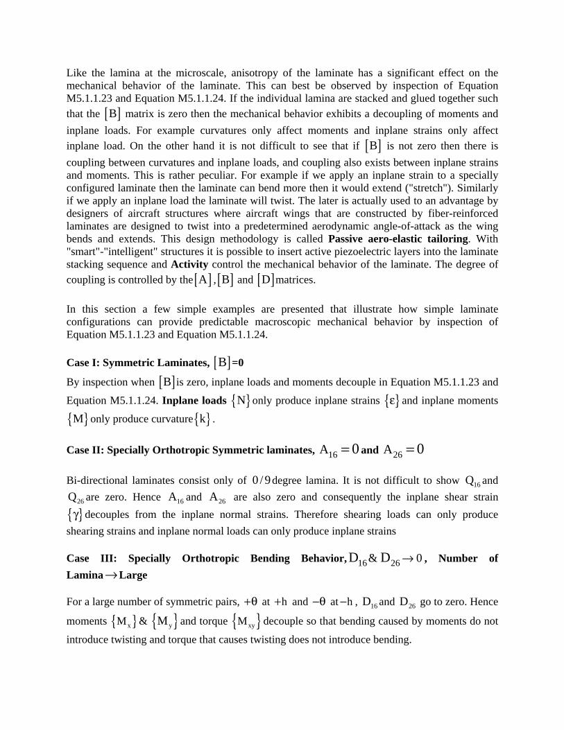
y only. As a result of these assumptions, the deformations can be described entirely in terms of the deformation of the mid-surface plane; hence, the plate is reduced to the study of a two-dimensional problem consisting of the plate mid-surface. Figure M5.1.2.2 shows the u and v displacement assumptions in the x-z and y-z planes respectively.

x-z plane

y-z plane

z

y w

v xwy

θ ∂=∂

z

x w

ywx

θ ∂=∂

u

Figure M5.1.2.2. Mid-plane Displacements

From Figure M5.1.2.2, the following displacement patterns may be assumed:

( , , ) ( , , 0) ( , )

( , , ) ( , ,0) ( , )( , , ) ( , ,0)

y

x

u x y z u x y z x y

v x y z v x y z x yw x y z w x y

θθ

= −

= −=

(M5.1.2.2)

where xwy

∂θ =∂

and ywx

∂θ =∂

are rotations of a normal the mid-plane about the x and negative y-

axes, respectively. M5.1.2.3 Stress Resultants In beam theory, the stress distribution that acts over a cross section may be integrated over the cross section to define equivalent forces and moments acting at the neutral axis. For two-dimensional plate analysis, it is more convenient to define stress resultants per unit length by integrating only through the thickness. Thus, stress resultants are defined to be forces and moments per unit length. The general stress components acting on an infinitesimal element are shown in Figure M5.1.2.3.

x y

z xxσ

xyσxzσ

yyσ

yxσ

yzσ

zzσ

zxσzyσ

note: stresses not shown all faces

xxσ

xyσxzσ

h

Figure M5.1.2.3. Free Body of Stress Components

The differential equations of equilibrium for an infinitesimal element in terms of stresses are given as below,

0

0

0

yxxx zx

xy yy zy

yzxz zz

Xx y z

Yx y z

Zx y z

σσ σ

σ σ σ

σσ σ

∂∂ ∂+ + + =∂ ∂ ∂

∂ ∂ ∂+ + + =

∂ ∂ ∂∂∂ ∂+ + + =

∂ ∂ ∂

(M5.1.2.3)

where X-, Y- and Z- are body forces per unit volume. In order to make the analysis easier, we define 8 stress resultants (forces and moments per unit length) by integrating through the thickness of the plate:

, ,

, ,

,

x xx y yy xy yx xyt t t

x xx y yy xy yx xyt t t

x xz y yzt t

N dz N dz N N dz

M z dz M z dz M M z dz

Q dz Q dz

σ σ σ

σ σ σ

σ σ

= = = =

= − = − = = −

= − = −

∫ ∫ ∫∫ ∫ ∫∫ ∫

(M5.1.2.4 (a))

These force and moment resultants are shown in Figure M5.1.2.4 (a) and Figure M5.1.2.4 (b).

Figure M5.1.2.4 (a). Force Stress Resultants

Figure M5.1.2.4 (b). Moment Stress Resultants

where xN and yN are in plane membrane forces per unit length (due to stretching of the plate mid surface), xM and yM are bending moments per unit length about the y and x axes, respectively, xQ and yQ are transverse shear forces per unit length, xyN is an in-plane shear force per unit length (same as shear flow in a shear panel), and xyM and yxM are twisting moments per unit length (similar to torsion in a beam). Note that you have to be careful about the sign convention for the forces and moments; some follow "usual" directions and notation, but some don't. For instance, the bending moment notation is opposite of what you normally think of ( xM is a bending moment about the y-axis!) and the shear forces xQ and yQ are opposite to the shear stresses. This notation and sign convention for force and moment resultants has been used for a long time in plate theory and is still used. M5.1.2.4 Equilibrium s in terms of Stress Resultants

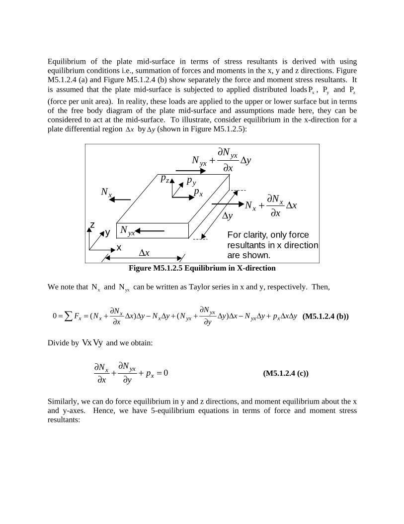
Equilibrium of the plate mid-surface in terms of stress resultants is derived with using equilibrium conditions i.e., summation of forces and moments in the x, y and z directions. Figure M5.1.2.4 (a) and Figure M5.1.2.4 (b) show separately the force and moment stress resultants. It is assumed that the plate mid-surface is subjected to applied distributed loads xP , yP and zP (force per unit area). In reality, these loads are applied to the upper or lower surface but in terms of the free body diagram of the plate mid-surface and assumptions made here, they can be considered to act at the mid-surface. To illustrate, consider equilibrium in the x-direction for a plate differential region x∆ by y∆ (shown in Figure M5.1.2.5):

x y

z

xN

yxN

xpypzp

x∆

y∆x

xNN xx

∂+ ∆∂

yxyx

NN y

x∂

+ ∆∂

For clarity, only force resultants in x direction are shown.

Figure M5.1.2.5 Equilibrium in X-direction We note that xN and yxN can be written as Taylor series in x and y, respectively. Then,

0 ( ) ( )yxxx x x yx yx x

NNF N x y N y N y x N y p x yx y

∂∂= = + ∆ ∆ − ∆ + + ∆ ∆ − ∆ + ∆ ∆∂ ∂∑

(M5.1.2.4 (b))

Divide by x yV V and we obtain:

0yxxx

NN px y

∂∂ + + =∂ ∂

(M5.1.2.4 (c))

Similarly, we can do force equilibrium in y and z directions, and moment equilibrium about the x and y-axes. Hence, we have 5-equilibrium equations in terms of force and moment stress resultants:

0

0

0

0

0

yxxx

xy yy

yxz

yxxx

xy yy

NN px y

N Np

x yQQ p

x yMM Q

x yM M

Qx y

∂∂ + + =∂ ∂

∂ ∂+ + =

∂ ∂∂∂ + − =

∂ ∂∂∂ − − =

∂ ∂∂ ∂

+ − =∂ ∂

(M5.1.2.5 (a))

M5.1.2.5 Strain-Displacement Relations As in beam theory, we will assume that all displacements and strains are small (infinitesimal). Similar to the assumptions made in Euler-Bernoulli beam theory, we assume displacement patterns of the mid-surface. Substituting these displacement assumptions into the infinitesimal strain-displacement equations, results in

2

2

2

2

2

( , ,0) ( , ,0)

( , ,0) ( , ,0)

( , ,0) ( , ,0) ( , ,0)2

xx

yy

xy

u u x y w x yzx x xv v x y w x yzy y y

u v u x y v x y w x yzy x y x x y

ε

ε

ε

∂ ∂ ∂= = −∂ ∂ ∂∂ ∂ ∂= = −∂ ∂ ∂

∂ ∂ ∂ ∂ ∂= + = + −∂ ∂ ∂ ∂ ∂ ∂

(M5.1.2.5b)

In the above expressions, all displacements are at the mid-surface and are functions of x and y only. To simply the notation, the functional notation of ( x, y,z ) will be dropped and the above expressions will be written as

2

2

2

2

22

xx

yy

xy

u u wzx x xv v wzy y y

u v u v wzy x y x x y

ε

ε

ε

∂ ∂ ∂= = −∂ ∂ ∂∂ ∂ ∂= = −∂ ∂ ∂

∂ ∂ ∂ ∂ ∂= + = + −∂ ∂ ∂ ∂ ∂ ∂

(M5.1.2.6)

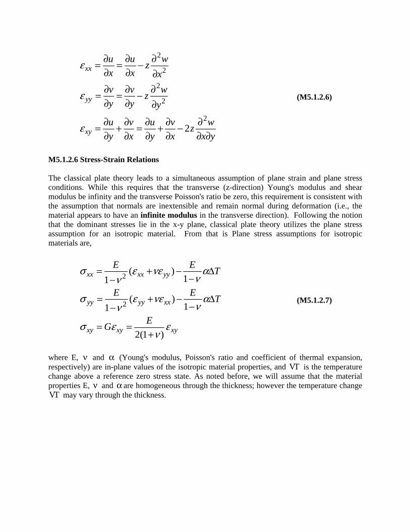
M5.1.2.6 Stress-Strain Relations The classical plate theory leads to a simultaneous assumption of plane strain and plane stress conditions. While this requires that the transverse (z-direction) Young's modulus and shear modulus be infinity and the transverse Poisson's ratio be zero, this requirement is consistent with the assumption that normals are inextensible and remain normal during deformation (i.e., the material appears to have an infinite modulus in the transverse direction). Following the notion that the dominant stresses lie in the x-y plane, classical plate theory utilizes the plane stress assumption for an isotropic material. From that is Plane stress assumptions for isotropic materials are,

2

2

( )11

( )11

2(1 )

xx xx yy

yy yy xx

xy xy xy

E E T

E E T

EG

σ ε νε ανν

σ ε νε ανν

σ ε εν

= + − ∆−−

= + − ∆−−

= =+

(M5.1.2.7)

where E, ν and α (Young's modulus, Poisson's ratio and coefficient of thermal expansion, respectively) are in-plane values of the isotropic material properties, and TV is the temperature change above a reference zero stress state. As noted before, we will assume that the material properties E, ν and α are homogeneous through the thickness; however the temperature change

TV may vary through the thickness.

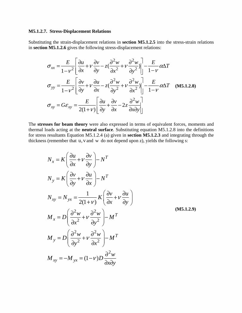
M5.1.2.7. Stress-Displacement Relations Substituting the strain-displacement relations in section M5.1.2.5 into the stress-strain relations in section M5.1.2.6 gives the following stress-displacement relations:

2 2

2 2 2

2 2

2 2 2

2

( )11

( )11

22(1 )

xx

yy

xy xy

E u v w w Ez Tx y x y

E v u w w Ez Ty x y x

E u v wG zy x x y

σ ν ν ανν

σ ν ν ανν

σ εν

⎡ ⎤∂ ∂ ∂ ∂= + − + − ∆⎢ ⎥∂ ∂ −− ∂ ∂⎢ ⎥⎣ ⎦⎡ ⎤∂ ∂ ∂ ∂= + − + − ∆⎢ ⎥∂ ∂ −− ∂ ∂⎢ ⎥⎣ ⎦

⎡ ⎤∂ ∂ ∂= = + −⎢ ⎥+ ∂ ∂ ∂ ∂⎢ ⎥⎣ ⎦

(M5.1.2.8)

The stresses for beam theory were also expressed in terms of equivalent forces, moments and thermal loads acting at the neutral surface. Substituting equation M5.1.2.8 into the definitions for stress resultants Equation M5.1.2.4 (a) given in section M5.1.2.3 and integrating through the thickness (remember that u, v and w do not depend upon z), yields the following s:

2 2

2 2

2 2

2 2

2

12(1 )

(1 )

Tx

Ty

xy yx

Tx

Ty

xy yx

u vN K Nx y

v uN K Ny x

v uN N Kx y

w wM D Mx y

w wM D My x

wM M Dx y

ν

ν

νν

ν

ν

ν

⎛ ⎞∂ ∂= + −⎜ ⎟∂ ∂⎝ ⎠⎛ ⎞∂ ∂= + −⎜ ⎟∂ ∂⎝ ⎠

⎛ ⎞∂ ∂= = +⎜ ⎟+ ∂ ∂⎝ ⎠⎛ ⎞∂ ∂= + −⎜ ⎟⎜ ⎟∂ ∂⎝ ⎠⎛ ⎞∂ ∂= + −⎜ ⎟⎜ ⎟∂ ∂⎝ ⎠

∂= − = −∂ ∂

(M5.1.2.9)

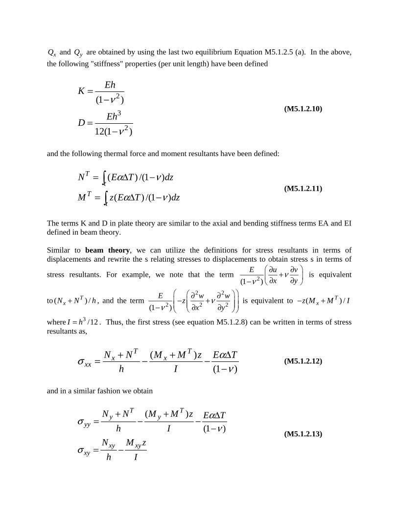
xQ and yQ are obtained by using the last two equilibrium Equation M5.1.2.5 (a). In the above, the following "stiffness" properties (per unit length) have been defined

2

3

2

(1 )

12(1 )

EhK

EhD

ν

ν

=−

=−

(M5.1.2.10)

and the following thermal force and moment resultants have been defined:

( ) /(1 )

( ) /(1 )

Tt

Tt

N E T dz

M z E T dz

α ν

α ν

= ∆ −

= ∆ −

∫∫

(M5.1.2.11)

The terms K and D in plate theory are similar to the axial and bending stiffness terms EA and EI defined in beam theory. Similar to beam theory, we can utilize the definitions for stress resultants in terms of displacements and rewrite the s relating stresses to displacements to obtain stress s in terms of

stress resultants. For example, we note that the term 2(1 )E u v

x yν

ν⎛ ⎞∂ ∂+⎜ ⎟∂ ∂− ⎝ ⎠

is equivalent

to ( ) /TxN N h+ , and the term

2 2

2 2 2(1 )E w wz

x yν

ν

⎛ ⎞⎛ ⎞∂ ∂− +⎜ ⎟⎜ ⎟⎜ ⎟⎜ ⎟− ∂ ∂⎝ ⎠⎝ ⎠ is equivalent to ( ) /T

xz M M I− +

where 3 /12I h= . Thus, the first stress (see equation M5.1.2.8) can be written in terms of stress resultants as,

( )(1 )

T Tx x

xxN N M M z E T

h Iασ

ν+ + ∆= − −

− (M5.1.2.12)

and in a similar fashion we obtain

( )(1 )

T Ty y

yy

xy xyxy

N N M M z E Th I

N M zh I

ασν

σ

+ + ∆= − −−

= −

(M5.1.2.13)

where I = moment of inertia (about the x- or y-axis) for a unit width of plate =

/ 2 2 3/ 2

/12h

hz dz h

−=∫ .

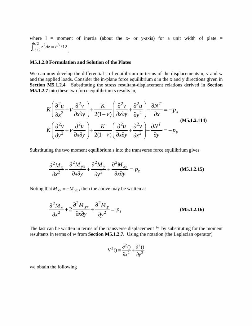
M5.1.2.8 Formulation and Solution of the Plates We can now develop the differential s of equilibrium in terms of the displacements u, v and w and the applied loads. Consider the in-plane force equilibrium s in the x and y directions given in Section M5.1.2.4. Substituting the stress resultant-displacement relations derived in Section M5.1.2.7 into these two force equilibrium s results in,

2 2 2 2

2 2

2 2 2 2

2 2

2(1 )

2(1 )

T

x

T

y

u v K v u NK px y x y xx y

v u K u v NK px y x y yy x

νν

νν

⎛ ⎞ ⎛ ⎞∂ ∂ ∂ ∂ ∂+ + + − = −⎜ ⎟ ⎜ ⎟⎜ ⎟ ⎜ ⎟∂ ∂ − ∂ ∂ ∂∂ ∂⎝ ⎠ ⎝ ⎠⎛ ⎞ ⎛ ⎞∂ ∂ ∂ ∂ ∂+ + + − = −⎜ ⎟ ⎜ ⎟⎜ ⎟ ⎜ ⎟∂ ∂ − ∂ ∂ ∂∂ ∂⎝ ⎠ ⎝ ⎠

(M5.1.2.114)

Substituting the two moment equilibrium s into the transverse force equilibrium gives

2 2 22

2 2yx y xyx

zM M MM px y x yx y

∂ ∂ ∂∂ − + + =∂ ∂ ∂ ∂∂ ∂

(M5.1.2.15)

Noting that xy yxM M= − , then the above may be written as

2 22

2 22 yx yxz

M MM px yx y

∂ ∂∂ + + =∂ ∂∂ ∂

(M5.1.2.16)

The last can be written in terms of the transverse displacement w by substituting for the moment resultants in terms of w from Section M5.1.2.7. Using the notation (the Laplacian operator)

2 22

2 2() ()()

x y∂ ∂∇ ≡ +∂ ∂

we obtain the following

2 2 22 2 2

2 22 2 2

2 2( ) (1 ) 2 Tz

w w wD D Dx yy x

D w p Mx yx y

ν

⎛ ⎞⎛ ⎞ ⎛ ⎞ ⎛ ⎞∂ ∂ ∂∂ ∂ ∂⎜ ⎟⎜ ⎟ ⎜ ⎟ ⎜ ⎟⎜ ⎟ ⎜ ⎟ ⎜ ⎟∂ ∂∂ ∂⎜ ⎟⎝ ⎠ ⎝ ⎠ ⎝ ⎠∇ ∇ − − + − = + ∇⎜ ⎟∂ ∂∂ ∂⎜ ⎟⎜ ⎟⎝ ⎠

(M5.1.2.17)

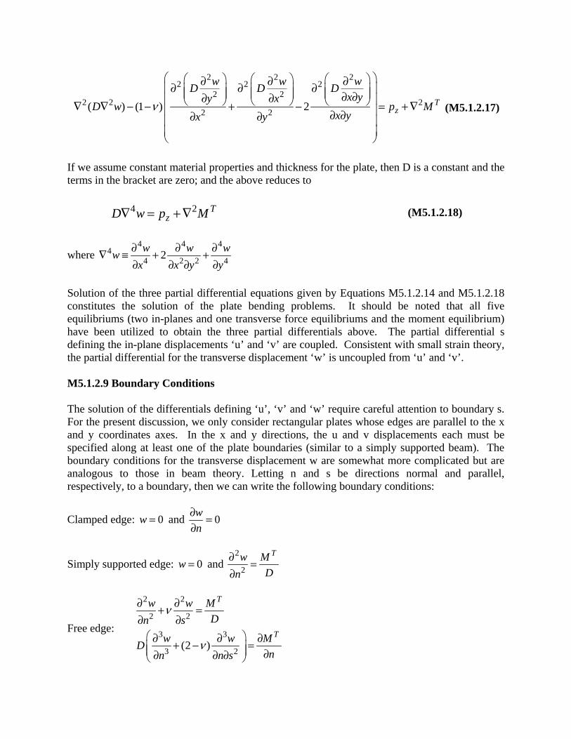
If we assume constant material properties and thickness for the plate, then D is a constant and the terms in the bracket are zero; and the above reduces to

4 2 TzD w p M∇ = + ∇ (M5.1.2.18)

where 4 4 4

44 2 2 42w w ww

x x y y∂ ∂ ∂∇ ≡ + +∂ ∂ ∂ ∂

Solution of the three partial differential equations given by Equations M5.1.2.14 and M5.1.2.18 constitutes the solution of the plate bending problems. It should be noted that all five equilibriums (two in-planes and one transverse force equilibriums and the moment equilibrium) have been utilized to obtain the three partial differentials above. The partial differential s defining the in-plane displacements ‘u’ and ‘v’ are coupled. Consistent with small strain theory, the partial differential for the transverse displacement ‘w’ is uncoupled from ‘u’ and ‘v’. M5.1.2.9 Boundary Conditions The solution of the differentials defining ‘u’, ‘v’ and ‘w’ require careful attention to boundary s. For the present discussion, we only consider rectangular plates whose edges are parallel to the x and y coordinates axes. In the x and y directions, the u and v displacements each must be specified along at least one of the plate boundaries (similar to a simply supported beam). The boundary conditions for the transverse displacement w are somewhat more complicated but are analogous to those in beam theory. Letting n and s be directions normal and parallel, respectively, to a boundary, then we can write the following boundary conditions:

Clamped edge: 0w = and 0wn

∂ =∂

Simply supported edge: 0w = and 2

2

Tw MDn

∂ =∂

Free edge:

2 2

2 2

3 3

3 2(2 )

T

T

w w MDn s

w w MDnn n s

ν

ν

∂ ∂+ =∂ ∂⎛ ⎞∂ ∂ ∂+ − =⎜ ⎟⎜ ⎟ ∂∂ ∂ ∂⎝ ⎠

The clamped boundary condition is equivalent to saying that the displacement and slope are zero. For the case of no thermal edge loads ( 0TM = ), the simply supported boundary condition requires that the displacement and curvature (i.e., the moment normal to the edge) be zero. The free edge boundary conditions require that the moment and shear be zero on the free edge (for the case of 0TM = ). When the thermal moment is not zero, the above s require that curvatures at the plate edge satisfy the above relations (i.e., the internal moment at the edge must equal the thermal moment TM (or its gradient for the shear boundary condition on a free edge). M5.1.2.10 Some Simple Plate Solutions The exact solution of the fourth-order, partial differential defining the transverse deflection w is generally quite difficult. For certain special cases, approximate analytical solutions can be obtained by assuming a displacement ( )w x, y and obtaining a particular and complimentary solution in the traditional manner of solving differential s. Other approximate solutions may be obtained by using finite difference or finite element methods. In practice, numerical finite difference methods (which replace derivatives by algebraic approximations) tend to cumbersome and difficult to apply for general plate geometries. The finite element method, which uses a combination of assumed displacement solutions and energy principles to solve the differential s, is better suited for arbitrary plate geometries. The finite element solution of plate problems will be considered in a later section. Consider the analytical solution of a thin, rectangular plate that has uniform material properties, is loaded with a uniform normal pressure op , and is simply supported along all edges. Assume the plate has dimensions ‘ a ’ and ‘b’ in the x- and y- directions, respectively, and that the coordinate system is located at one corner of the plate as shown in Figure M5.1.2.6.

x

y

a

b p o

Figure M5.1.2.6 Coordinate system of Plate

Since the thermal loading is assumed to be zero, we are faced with solving the following fourth-order differential,

4zD w p∇ =

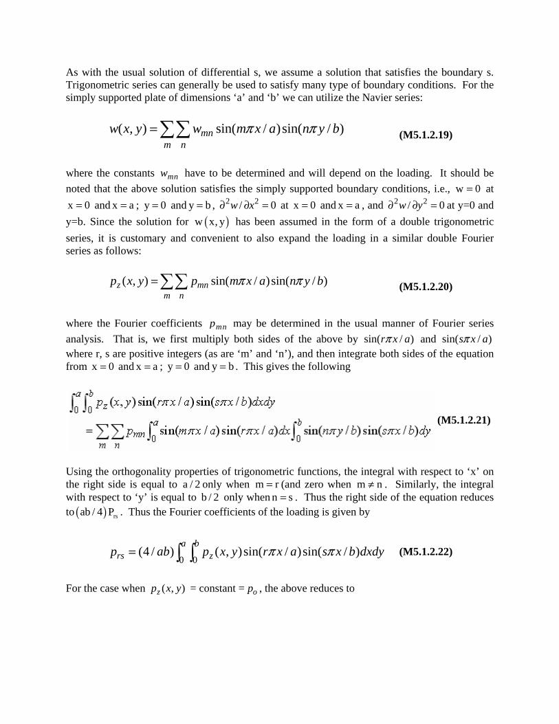
As with the usual solution of differential s, we assume a solution that satisfies the boundary s. Trigonometric series can generally be used to satisfy many type of boundary conditions. For the simply supported plate of dimensions ‘a’ and ‘b’ we can utilize the Navier series:

( , ) sin( / )sin( / )mnm n

w x y w m x a n y bπ π=∑∑

(M5.1.2.19)

where the constants mnw have to be determined and will depend on the loading. It should be noted that the above solution satisfies the simply supported boundary conditions, i.e., w 0= at x 0= and x a= ; y 0= and y b= , 2 2/ 0w x∂ ∂ = at x 0= and x a= , and 2 2/ 0w y∂ ∂ = at y=0 and y=b. Since the solution for ( )w x, y has been assumed in the form of a double trigonometric series, it is customary and convenient to also expand the loading in a similar double Fourier series as follows:

( , ) sin( / )sin( / )z mnm n

p x y p m x a n y bπ π=∑∑

(M5.1.2.20)

where the Fourier coefficients mnp may be determined in the usual manner of Fourier series analysis. That is, we first multiply both sides of the above by sin( / )r x aπ and sin( / )s x aπ where r, s are positive integers (as are ‘m’ and ‘n’), and then integrate both sides of the equation from x 0= and x a= ; y 0= and y b= . This gives the following

(M5.1.2.21)

Using the orthogonality properties of trigonometric functions, the integral with respect to ‘x’ on the right side is equal to a / 2 only when m r= (and zero when m n≠ . Similarly, the integral with respect to ‘y’ is equal to b / 2 only when n s= . Thus the right side of the equation reduces to ( ) rsab / 4 P . Thus the Fourier coefficients of the loading is given by

0 0(4 / ) ( , )sin( / )sin( / )

a brs zp ab p x y r x a s x b dxdyπ π= ∫ ∫

(M5.1.2.22)

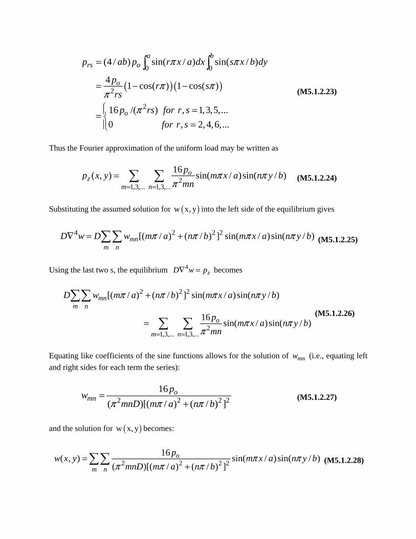
For the case when ( , )zp x y = constant = op , the above reduces to

( ) ( )0 0

2

2

(4 / ) sin( / ) sin( / )

4 1 cos( ) 1 cos( )

16 /( ) , 1,3,5,... 0 , 2, 4,6,...

a brs o

o

o

p ab p r x a dx s x b dy

p r srsp rs for r s

for r s

π π

π ππ

π

=

= − −

⎧ =⎪= ⎨=⎪⎩

∫ ∫

(M5.1.2.23)

Thus the Fourier approximation of the uniform load may be written as

21,3,... 1,3,...

16( , ) sin( / )sin( / )oz

m n

pp x y m x a n y bmn

π ππ= =

= ∑ ∑

(M5.1.2.24)

Substituting the assumed solution for ( )w x, y into the left side of the equilibrium gives

4 2 2 2[( / ) ( / ) ] sin( / )sin( / )mnm n

D w D w m a n b m x a n y bπ π π π∇ = +∑∑ (M5.1.2.25)

Using the last two s, the equilibrium 4

zD w p∇ = becomes

2 2 2

21,3,... 1,3,...

[( / ) ( / ) ] sin( / )sin( / )

16 sin( / )sin( / )

mnm n

o

m n

D w m a n b m x a n y b

p m x a n y bmn

π π π π

π ππ= =

+

=

∑∑

∑ ∑

(M5.1.2.26)

Equating like coefficients of the sine functions allows for the solution of mnw (i.e., equating left and right sides for each term the series):

2 2 2 216

( )[( / ) ( / ) ]o

mnpw

mnD m a n bπ π π=

+ (M5.1.2.27)

and the solution for ( )w x, y becomes:

2 2 2 216( , ) sin( / ) sin( / )

( )[( / ) ( / ) ]o

m n

pw x y m x a n y bmnD m a n b

π ππ π π

=+

∑∑ (M5.1.2.28)

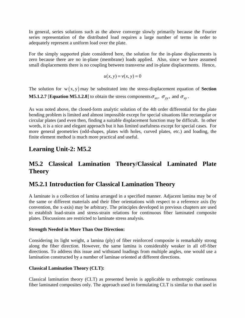
In general, series solutions such as the above converge slowly primarily because the Fourier series representation of the distributed load requires a large number of terms in order to adequately represent a uniform load over the plate. For the simply supported plate considered here, the solution for the in-plane displacements is zero because there are no in-plane (membrane) loads applied. Also, since we have assumed small displacements there is no coupling between transverse and in-plane displacements. Hence,

( , ) ( , ) 0u x y v x y= = The solution for ( )w x, y may be substituted into the stress-displacement equation of Section M5.1.2.7 [Equation M5.1.2.8] to obtain the stress components , , and xx yy xyσ σ σ . As was noted above, the closed-form analytic solution of the 4th order differential for the plate bending problem is limited and almost impossible except for special situations like rectangular or circular plates (and even then, finding a suitable displacement function may be difficult. In other words, it is a nice and elegant approach but it has limited usefulness except for special cases. For more general geometries (odd-shapes, plates with holes, curved plates, etc.) and loading, the finite element method is much more practical and useful. Learning Unit-2: M5.2 M5.2 Classical Lamination Theory/Classical Laminated Plate Theory M5.2.1 Introduction for Classical Lamination Theory A laminate is a collection of lamina arranged in a specified manner. Adjacent lamina may be of the same or different materials and their fiber orientations with respect to a reference axis (by convention, the x-axis) may be arbitrary. The principles developed in previous chapters are used to establish load-strain and stress-strain relations for continuous fiber laminated composite plates. Discussions are restricted to laminate stress analysis. Strength Needed in More Than One Direction: Considering its light weight, a lamina (ply) of fiber reinforced composite is remarkably strong along the fiber direction. However, the same lamina is considerably weaker in all off-fiber directions. To address this issue and withstand loadings from multiple angles, one would use a lamination constructed by a number of laminae oriented at different directions. Classical Lamination Theory (CLT): Classical lamination theory (CLT) as presented herein is applicable to orthotropic continuous fiber laminated composites only. The approach used in formulating CLT is similar to that used in

developing load-stress relationships in elementary strength of materials courses. An initial displacement field consistent with applied loads is assumed. Through the strain-displacement fields and an appropriate constitutive relationship, a state of stress is defined. By satisfying the conditions of static equilibrium, a load-strain relation is defined, and subsequently a state of stress is defined for each lamina. M5.2.1.1 Basic Assumptions of Classical Lamination Theory Similar to the Euler-Bernoulli beam theory and the plate theory, the classical lamination theory is only valid for thin laminates (span ‘a’ and ‘b’ > 10×thinckness ‘t’) with small displacement ‘w’ in the transverse direction (w << t). It shares the same classical plate theory assumptions: Kirchhoff’s Hypothesis:

1. Normals remain straight (they do not bend) 2. Normals remain unstretched (they keep the same length) 3. Normals remain normal (they always make a right angle to the neutral plane)

In addition, perfect bonding between layers is assumed. Perfect Bonding:

1. The bonding itself is infinitesimally small (there is no flaw or gap between layers). 2. The bonding is non-shear-deformable (no lamina can slip relative to another). 3. The strength of bonding is as strong as it needs to be (the laminate acts as a single lamina

with special integrated properties). Basic Assumptions for Classical Lamination Theory (CLT):

1. Each layer of the laminate is quasi-homogeneous and orthotropic. 2. The laminate is thin compared to the lateral dimensions and is loaded in its plane. 3. State of stress is plane stress. 4. All displacements are small compared to the laminate thickness. 5. Displacements are continuous throughout the laminate. 6. Straight lines normal to the middle surface remain straight and normal to that surface

after deformation. • In-plane displacements vary linearly through the thickness, • Transverse shear strains ( xz yz&γ γ ) are negligible.

7. Transverse normal strain zε is negligible compared to the in-plane strains xε and yε . 8. Strain-displacement and stress-strain relations are linear.

M5.2.1.2 Classical Lamination Theory from Classical Plate Theory: The classical lamination theory is almost identical to the classical plate theory; the only difference is in the material properties (stress-strain relations). The classical plate theory usually

assumes that the material is isotropic, while a fiber reinforced composite laminate with multiple layers (plies) may have more complicated stress-strain relations. The four cornerstones of the lamination theory are the kinematic, constitutive, force resultant, and equilibrium equations. The outcome of each of these segments is summarized as follows: M5.2.1.2.1 Kinematics Equations: Kinematics describes how the plate's displacements and strains relate:

(M5.2.1.1)

where ‘u’, ‘v’, and ‘w’ are the displacement in x-, y-, and z-direction, respectively. That is,

(M5.2.1.2)

where 0 0u , v , and 0w are the displacements of the middle plane in the x-, y-, and z-directions, respectively. Please note that some literature may define xyκ as the total skew curvature which eliminates the factor of 2. Also note that Kirchhoff's assumptions are introduced to simplify the displacement fields. M5.2.1.2.2 Constitutive Equations: Hooke's Law:

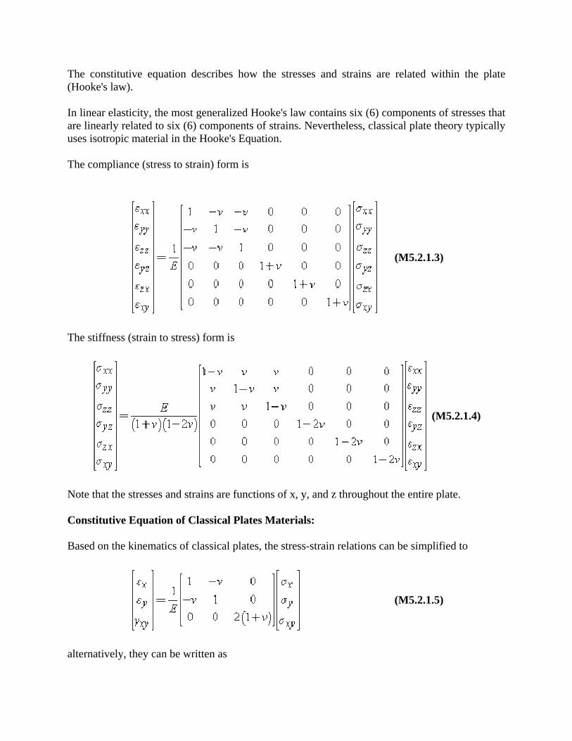
The constitutive equation describes how the stresses and strains are related within the plate (Hooke's law). In linear elasticity, the most generalized Hooke's law contains six (6) components of stresses that are linearly related to six (6) components of strains. Nevertheless, classical plate theory typically uses isotropic material in the Hooke's Equation. The compliance (stress to strain) form is

(M5.2.1.3)

The stiffness (strain to stress) form is

(M5.2.1.4)

Note that the stresses and strains are functions of x, y, and z throughout the entire plate. Constitutive Equation of Classical Plates Materials: Based on the kinematics of classical plates, the stress-strain relations can be simplified to

(M5.2.1.5)

alternatively, they can be written as

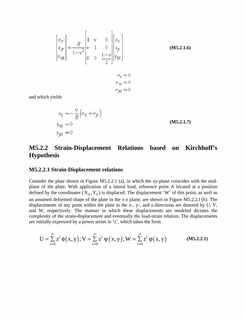
(M5.2.1.6)

and which yields

(M5.2.1.7)

M5.2.2 Strain-Displacement Relations based on Kirchhoff’s Hypothesis M5.2.2.1 Strain-Displacement relations Consider the plate shown in Figure M5.2.2.1 (a), in which the xy-plane coincides with the mid-plane of the plate. With application of a lateral load, reference point A located at a position defined by the coordinates ( A AX ,Y ) is displaced. The displacement ‘W’ of this point, as well as an assumed deformed shape of the plate in the x-z plane, are shown in Figure M5.2.2.l (b). The displacements of any point within the plate in the x-, y-, and z-directions are denoted by U, V, and W, respectively. The manner in which these displacements are modeled dictates the complexity of the strain-displacement and eventually the load-strain relation. The displacements are initially expressed by a power series in ‘z’, which takes the form

( ) ( ) ( )i i i

i 0 i 0 i 0U z x, y ;V z x, y ; W z x, y

∞ ∞ ∞

= = == ∑ φ = ∑ ψ = ∑ ϕ (M5.2.2.1)

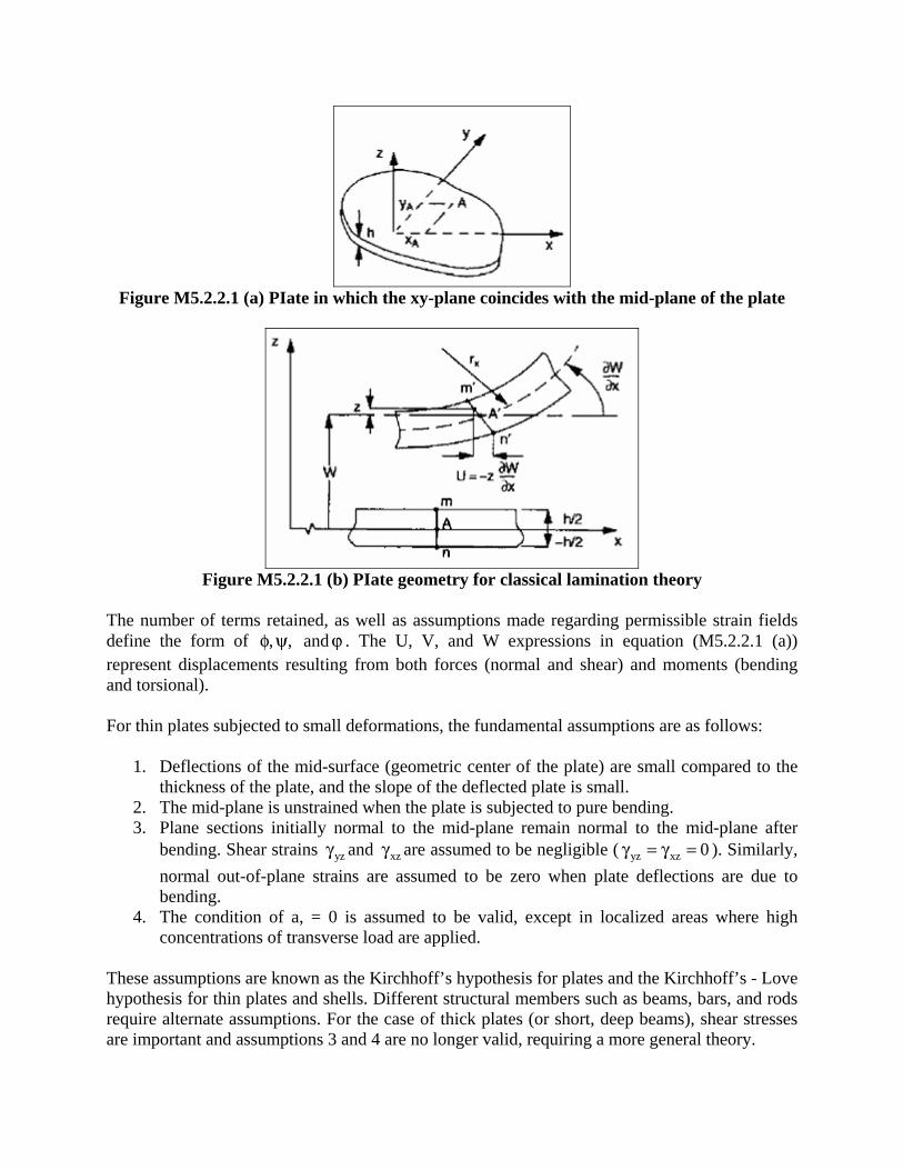
Figure M5.2.2.1 (a) PIate in which the xy-plane coincides with the mid-plane of the plate

Figure M5.2.2.1 (b) PIate geometry for classical lamination theory

The number of terms retained, as well as assumptions made regarding permissible strain fields define the form of , ,φ ψ and ϕ . The U, V, and W expressions in equation (M5.2.2.1 (a)) represent displacements resulting from both forces (normal and shear) and moments (bending and torsional). For thin plates subjected to small deformations, the fundamental assumptions are as follows:

1. Deflections of the mid-surface (geometric center of the plate) are small compared to the thickness of the plate, and the slope of the deflected plate is small.

2. The mid-plane is unstrained when the plate is subjected to pure bending. 3. Plane sections initially normal to the mid-plane remain normal to the mid-plane after

bending. Shear strains yzγ and xzγ are assumed to be negligible ( yz xz 0γ = γ = ). Similarly, normal out-of-plane strains are assumed to be zero when plate deflections are due to bending.

4. The condition of a, = 0 is assumed to be valid, except in localized areas where high concentrations of transverse load are applied.

These assumptions are known as the Kirchhoff’s hypothesis for plates and the Kirchhoff’s - Love hypothesis for thin plates and shells. Different structural members such as beams, bars, and rods require alternate assumptions. For the case of thick plates (or short, deep beams), shear stresses are important and assumptions 3 and 4 are no longer valid, requiring a more general theory.

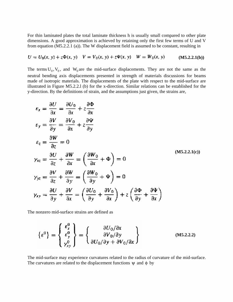
For thin laminated plates the total laminate thickness h is usually small compared to other plate dimensions. A good approximation is achieved by retaining only the first few terms of U and V from equation (M5.2.2.1 (a)). The W displacement field is assumed to be constant, resulting in

(M5.2.2.1(b)) The terms 0 0U , V , and 0W are the mid-surface displacements. They are not the same as the neutral bending axis displacements presented in strength of materials discussions for beams made of isotropic materials. The displacements of the plate with respect to the mid-surface are illustrated in Figure M5.2.2.l (b) for the x-direction. Similar relations can be established for the y-direction. By the definitions of strain, and the assumptions just given, the strains are,

(M5.2.2.1(c))

The nonzero mid-surface strains are defined as

(M5.2.2.2)

The mid-surface may experience curvatures related to the radius of curvature of the mid-surface. The curvatures are related to the displacement functions ψ and φ by

(M5.2.2.3)

Each term in equation (M5.2.2.3) can be related to a radius of curvature of the plate. Each curvature and its associated relationship to ψ and φ is illustrated in Figure M5.2.2.2. The strain variation through a laminate is expressed by a combination of equations (M5.2.2.2) and (M5.2.2.3) as,

(M5.2.2.4)

Figure M5.2.2.2 Plate curvatures for classical lamination theory

The strains in equation (M5.2.2.4) are valid for conditions of plane stress ( yz xz z 0γ = γ = σ = ). In cases where the condition on the two shear strains being zero is relaxed, the strain relationship given by equation (M5.2.2.4) contains additional terms ( xzγ and yzγ ), which are not functions of the curvatures x y, ,κ κ and xyκ .

With xzγ and yzγ zero, ψ and φ can be explicitly defined in terms of 0W from the strain-displacement relations as

(M5.2.2.5)

It follows directly from equation (M5.2.2.3) that the curvatures are,

(M5.2.2.6 (a))

Using these definitions of curvature and equation (M5.2.2.2), the strain variation through the laminate as represented by equation (M5.2.2.4) can be expressed in terms of displacements. This form of the strain variation is convenient for problems in which deflections are required. Examples of such problems are generally found with beams, plate and shell vibrations, etc., where φ and ψ are obtained from boundary and initial conditions. They are not considered herein. M5.2.2.2 Stress-Strain Relationships The strain variation through a laminate is a function of both mid-surface strain and curvature and is continuous through the plate thickness. The stress need not be continuous through the plate. Consider the plane stress relationship between Cartesian stresses and strains,

(M5.2.2.6 (b))

Each lamina through the thickness may have a different fiber orientation and consequently a different Q⎡ ⎤⎣ ⎦ .The stress variation through the laminate thickness is therefore discontinuous.

This is illustrated by considering a simple one-dimensional model. Assume a laminate is subjected to a uniform strain xε , (with all other strains assumed to be zero). The stress in the x-

direction is related to the strain by 11Q . This component of 11Q⎡ ⎤⎣ ⎦ is not constant through the

laminate thickness. The magnitude of 11Q related to the fiber orientation of each lamina in the laminate. As illustrated in Figure M5.2.2.3, the linear variation of strain combined with

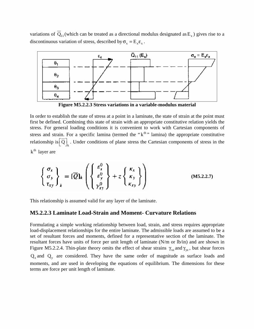
variations of 11Q (which can be treated as a directional modulus designated as xE ) gives rise to a discontinuous variation of stress, described by x x xEσ = ε .

Figure M5.2.2.3 Stress variations in a variable-modulus material

In order to establish the state of stress at a point in a laminate, the state of strain at the point must first be defined. Combining this state of strain with an appropriate constitutive relation yields the stress. For general loading conditions it is convenient to work with Cartesian components of stress and strain. For a specific lamina (termed the “ thk ” lamina) the appropriate constitutive relationship is

kQ⎡ ⎤⎣ ⎦ . Under conditions of plane stress the Cartesian components of stress in the

thk layer are

(M5.2.2.7)

This relationship is assumed valid for any layer of the laminate. M5.2.2.3 Laminate Load-Strain and Moment- Curvature Relations Formulating a simple working relationship between load, strain, and stress requires appropriate load-displacement relationships for the entire laminate. The admissible loads are assumed to be a set of resultant forces and moments, defined for a representative section of the laminate. The resultant forces have units of force per unit length of laminate (N/m or lb/in) and are shown in Figure M5.2.2.4. Thin-plate theory omits the effect of shear strains xzγ and yzγ , but shear forces

xQ and yQ are considered. They have the same order of magnitude as surface loads and moments, and are used in developing the equations of equilibrium. The dimensions for these terms are force per unit length of laminate.

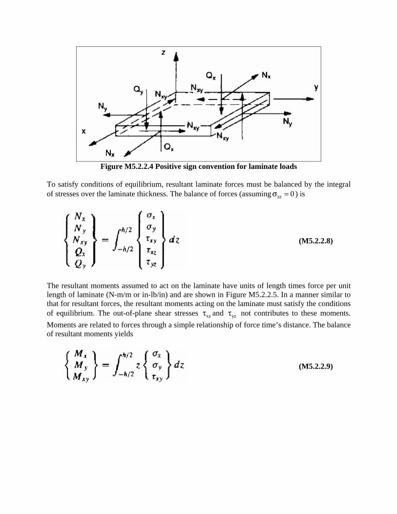
Figure M5.2.2.4 Positive sign convention for laminate loads

To satisfy conditions of equilibrium, resultant laminate forces must be balanced by the integral of stresses over the laminate thickness. The balance of forces (assuming zz 0σ = ) is

(M5.2.2.8)

The resultant moments assumed to act on the laminate have units of length times force per unit length of laminate (N-m/m or in-lb/in) and are shown in Figure M5.2.2.5. In a manner similar to that for resultant forces, the resultant moments acting on the laminate must satisfy the conditions of equilibrium. The out-of-plane shear stresses xzτ and yzτ not contributes to these moments. Moments are related to forces through a simple relationship of force time’s distance. The balance of resultant moments yields

(M5.2.2.9)

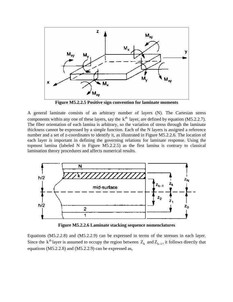
Figure M5.2.2.5 Positive sign convention for laminate moments

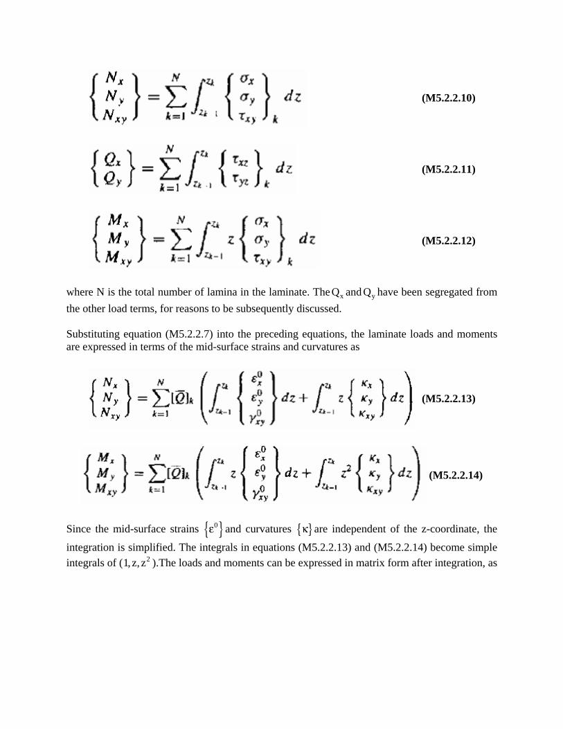
A general laminate consists of an arbitrary number of layers (N). The Cartesian stress components within any one of these layers, say the thk layer, are defined by equation (M5.2.2.7). The fiber orientation of each lamina is arbitrary, so the variation of stress through the laminate thickness cannot be expressed by a simple function. Each of the N layers is assigned a reference number and a set of z-coordinates to identify it, as illustrated in Figure M5.2.2.6. The location of each layer is important in defining the governing relations for laminate response. Using the topmost lamina (labeled N in Figure M5.2.2.5) as the first lamina is contrary to classical lamination theory procedures and affects numerical results.

Figure M5.2.2.6 Laminate stacking sequence nomenclatures

Equations (M5.2.2.8) and (M5.2.2.9) can be expressed in terms of the stresses in each layer. Since the thk layer is assumed to occupy the region between kZ and k 1Z − , it follows directly that equations (M5.2.2.8) and (M5.2.2.9) can be expressed as,

(M5.2.2.10)

(M5.2.2.11)

(M5.2.2.12)

where N is the total number of lamina in the laminate. The xQ and yQ have been segregated from the other load terms, for reasons to be subsequently discussed. Substituting equation (M5.2.2.7) into the preceding equations, the laminate loads and moments are expressed in terms of the mid-surface strains and curvatures as

(M5.2.2.13)

(M5.2.2.14)

Since the mid-surface strains { }0ε and curvatures { }κ are independent of the z-coordinate, the

integration is simplified. The integrals in equations (M5.2.2.13) and (M5.2.2.14) become simple integrals of ( 21, z, z ).The loads and moments can be expressed in matrix form after integration, as

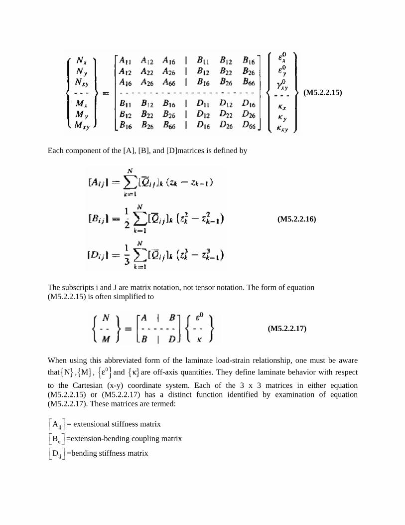
(M5.2.2.15)

Each component of the [A], [B], and [D]matrices is defined by

(M5.2.2.16)

The subscripts i and J are matrix notation, not tensor notation. The form of equation (M5.2.2.15) is often simplified to

(M5.2.2.17)

When using this abbreviated form of the laminate load-strain relationship, one must be aware that{ }N ,{ }M , { }0ε and { }κ are off-axis quantities. They define laminate behavior with respect

to the Cartesian (x-y) coordinate system. Each of the 3 x 3 matrices in either equation (M5.2.2.15) or (M5.2.2.17) has a distinct function identified by examination of equation (M5.2.2.17). These matrices are termed:

ijA⎡ ⎤⎣ ⎦ = extensional stiffness matrix

ijB⎡ ⎤⎣ ⎦ =extension-bending coupling matrix

ijD⎡ ⎤⎣ ⎦ =bending stiffness matrix

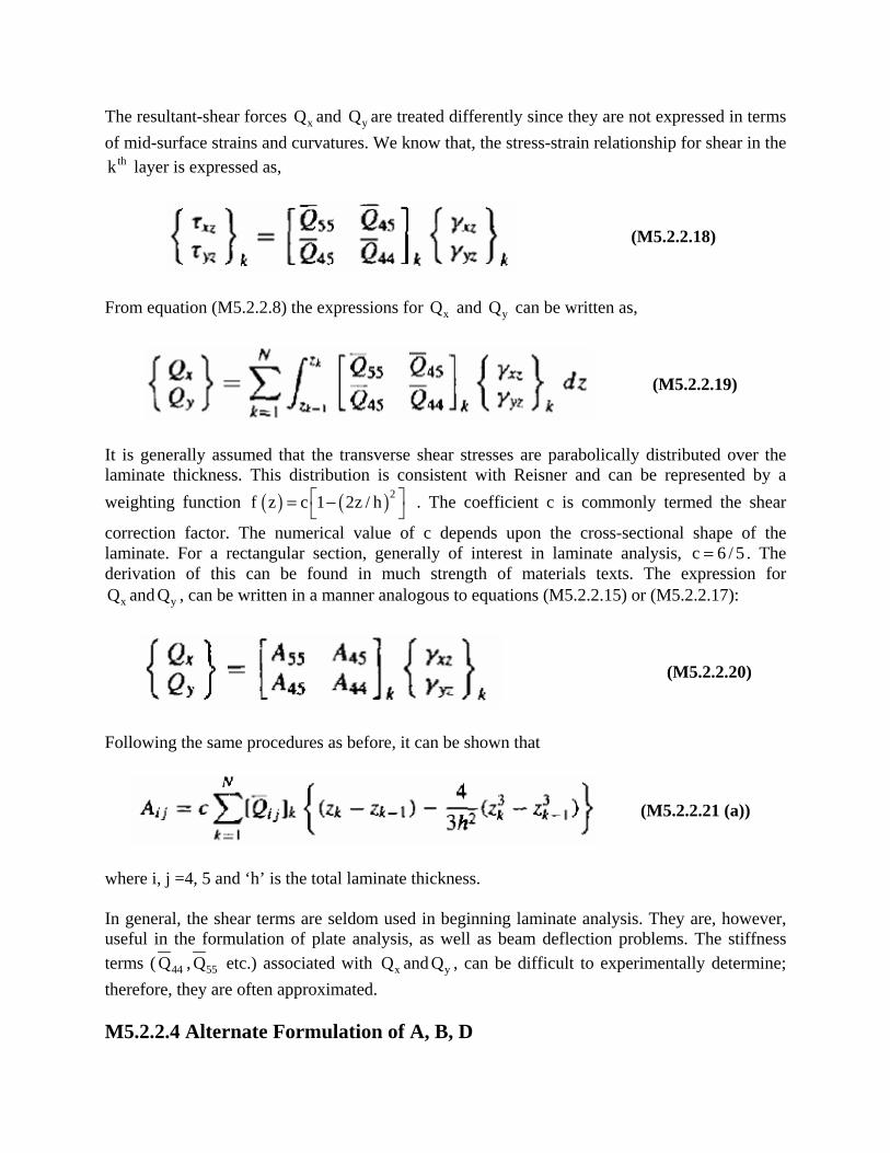
The resultant-shear forces xQ and yQ are treated differently since they are not expressed in terms of mid-surface strains and curvatures. We know that, the stress-strain relationship for shear in the

thk layer is expressed as,

(M5.2.2.18)

From equation (M5.2.2.8) the expressions for xQ and yQ can be written as,

(M5.2.2.19)

It is generally assumed that the transverse shear stresses are parabolically distributed over the laminate thickness. This distribution is consistent with Reisner and can be represented by a weighting function ( ) ( )2f z c 1 2z / h⎡ ⎤= −⎣ ⎦ . The coefficient c is commonly termed the shear

correction factor. The numerical value of c depends upon the cross-sectional shape of the laminate. For a rectangular section, generally of interest in laminate analysis, c 6 / 5= . The derivation of this can be found in much strength of materials texts. The expression for

xQ and yQ , can be written in a manner analogous to equations (M5.2.2.15) or (M5.2.2.17):

(M5.2.2.20)

Following the same procedures as before, it can be shown that

(M5.2.2.21 (a))

where i, j =4, 5 and ‘h’ is the total laminate thickness. In general, the shear terms are seldom used in beginning laminate analysis. They are, however, useful in the formulation of plate analysis, as well as beam deflection problems. The stiffness terms ( 44Q , 55Q etc.) associated with xQ and yQ , can be difficult to experimentally determine; therefore, they are often approximated. M5.2.2.4 Alternate Formulation of A, B, D

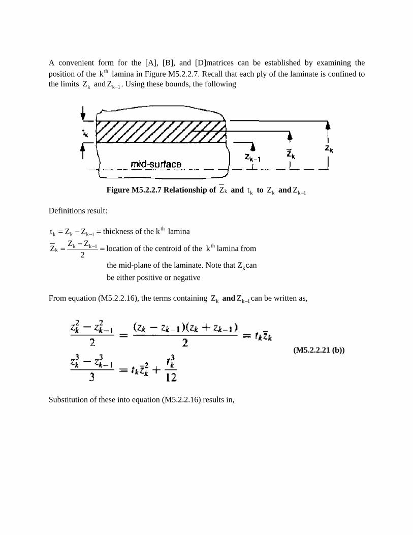
A convenient form for the [A], [B], and [D]matrices can be established by examining the position of the thk lamina in Figure M5.2.2.7. Recall that each ply of the laminate is confined to the limits kZ and k 1Z − . Using these bounds, the following

Figure M5.2.2.7 Relationship of kZ and kt to kZ and k 1Z −

Definitions result:

thk k k 1t Z Z thickness of the k lamina −= − =

th k k 1k

k

Z ZZ location of the centroid of the k lamina from 2

the mid-plane of the laminate. Note that Z can be either positive or negative

−−= =

From equation (M5.2.2.16), the terms containing kZ and k 1Z − can be written as,

(M5.2.2.21 (b))

Substitution of these into equation (M5.2.2.16) results in,

(M5.2.2.22)

For transverse shear the analogous expression is

(M5.2.2.23 (a))

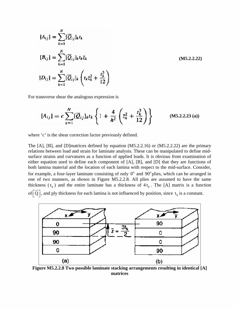
where ‘c’ is the shear correction factor previously defined. The [A], [B], and [D]matrices defined by equation (M5.2.2.16) or (M5.2.2.22) are the primary relations between load and strain for laminate analysis. These can be manipulated to define mid-surface strains and curvatures as a function of applied loads. It is obvious from examination of either equation used to define each component of [A], [B], and [D] that they are functions of both lamina material and the location of each lamina with respect to the mid-surface. Consider, for example, a four-layer laminate consisting of only 0o and 90o plies, which can be arranged in one of two manners, as shown in Figure M5.2.2.8. All plies are assumed to have the same thickness ( kt ) and the entire laminate has a thickness of 4 kt . The [A] matrix is a function

of Q⎡ ⎤⎣ ⎦ , and ply thickness for each lamina is not influenced by position, since kt is a constant.

Figure M5.2.2.8 Two possible laminate stacking arrangements resulting in identical [A]

matrices

The [D] matrix is influenced by kt , and, and Q⎡ ⎤⎣ ⎦ for each lamina. Considering only 11D ,

equation (M5.2.2.22) for this term is

(M5.2.2.23 (b))

11D for the laminate of Figure M5.2.2.8 (a) and Figure M5.2.2.8 (b) is

(M5.2.2.23(c))

Since, 11 110 90

Q Q⎡ ⎤ ⎡ ⎤>⎣ ⎦ ⎣ ⎦ the laminate in Figure M5.2.2.8 (a) has a larger 11D than that of Figure

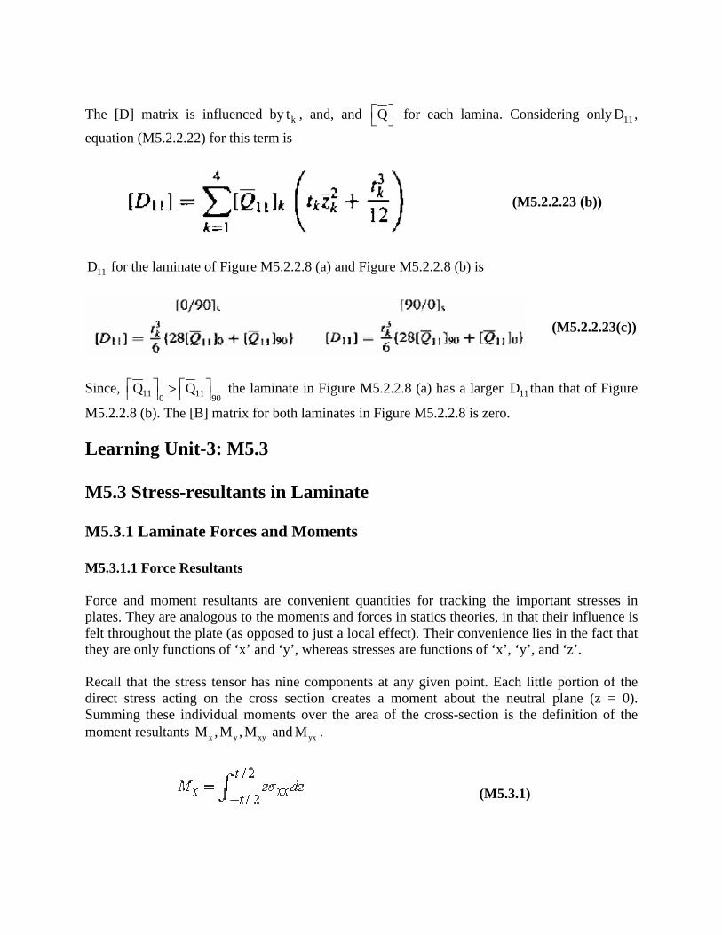
M5.2.2.8 (b). The [B] matrix for both laminates in Figure M5.2.2.8 is zero. Learning Unit-3: M5.3 M5.3 Stress-resultants in Laminate M5.3.1 Laminate Forces and Moments M5.3.1.1 Force Resultants Force and moment resultants are convenient quantities for tracking the important stresses in plates. They are analogous to the moments and forces in statics theories, in that their influence is felt throughout the plate (as opposed to just a local effect). Their convenience lies in the fact that they are only functions of ‘x’ and ‘y’, whereas stresses are functions of ‘x’, ‘y’, and ‘z’. Recall that the stress tensor has nine components at any given point. Each little portion of the direct stress acting on the cross section creates a moment about the neutral plane (z = 0). Summing these individual moments over the area of the cross-section is the definition of the moment resultants x y xyM ,M ,M and yxM .

(M5.3.1)

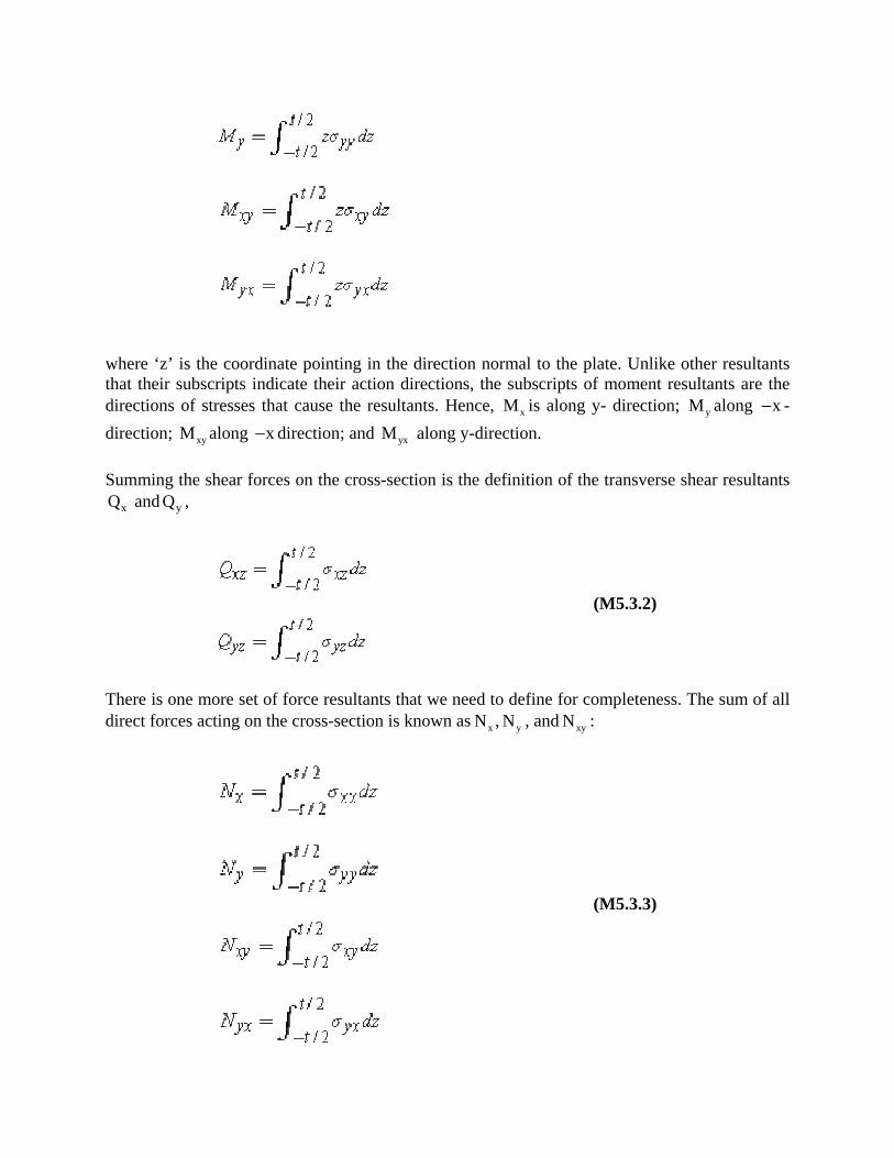
where ‘z’ is the coordinate pointing in the direction normal to the plate. Unlike other resultants that their subscripts indicate their action directions, the subscripts of moment resultants are the directions of stresses that cause the resultants. Hence, xM is along y- direction; yM along x− -direction; xyM along x− direction; and yxM along y-direction. Summing the shear forces on the cross-section is the definition of the transverse shear resultants

xQ and yQ ,

(M5.3.2)

There is one more set of force resultants that we need to define for completeness. The sum of all direct forces acting on the cross-section is known as x yN , N , and xyN :

(M5.3.3)

x y xyN , N , N , and yxN are the total in-plane normal and shear forces within the plate at some point (x, y), yet they do not play a role in (linear) plate theory since they do not cause a displacement ‘w’. These force and moment resultants should be in equilibrium with all external forces and moments. M5.3.1.2 Equilibrium Equations/Force Equilibrium: The equilibrium equations describe how the plate carries external pressure loads with its internal stresses. To enforce equilibrium, consider the balance of forces and moments acting on a small section of plate. There are six (6) equilibrium equations, three for the forces and three for the moments, which need to be satisfied. The equations of force equilibrium are

x-direction:

y-direction:

z-direction:

where x y xy yx xzN , N , N , N ,Q and yzQ are force resultants; x yp , p and zp are distributed external forces applied on the plate. The equations of moment equilibrium are

x-direction:

y-direction:

z-direction:

where x y xy yx xyM ,M ,M ,M , N and yxN are moment resultants; and x y zm ,m ,m are distributed external moments applied on the plate.

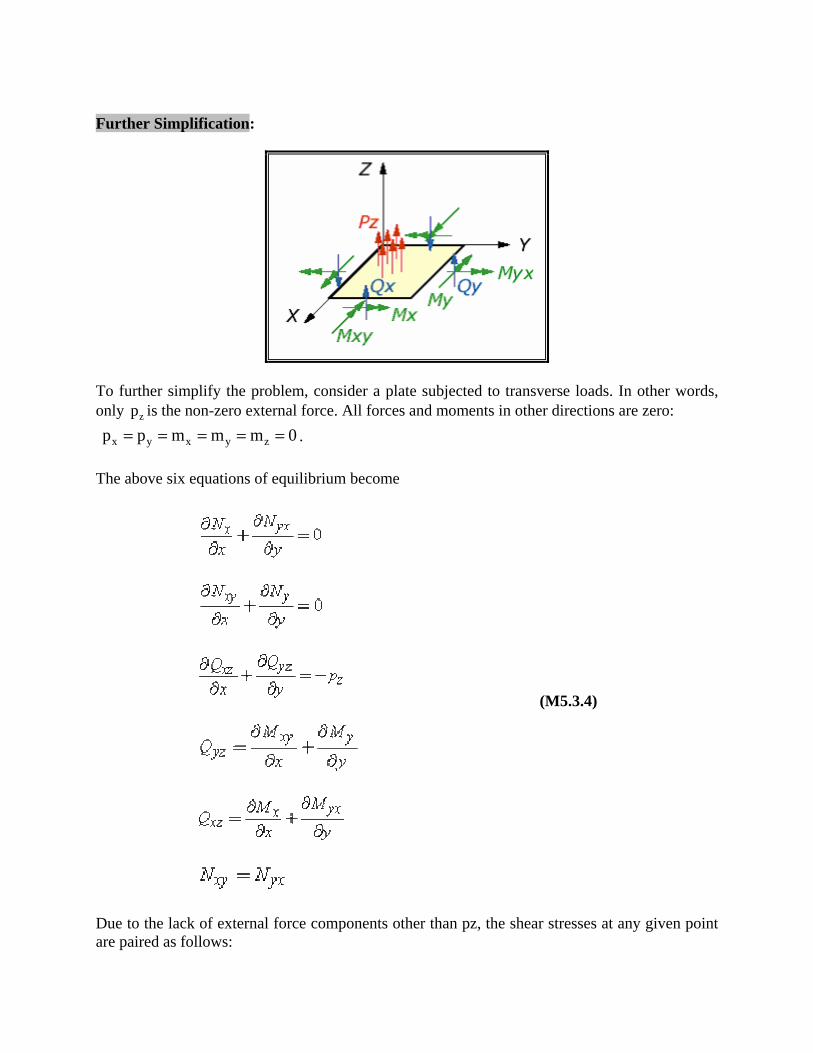
Further Simplification:

To further simplify the problem, consider a plate subjected to transverse loads. In other words, only zp is the non-zero external force. All forces and moments in other directions are zero: x y x y zp p m m m 0= = = = = . The above six equations of equilibrium become

(M5.3.4)

Due to the lack of external force components other than pz, the shear stresses at any given point are paired as follows:

(M5.3.5)

This yield,

(M5.3.6)

M5.3.2 Limitations of the Classic Laminate Theory: The classic laminate theory (CLT) is the simplest laminate theory one can get. While it has a reasonable range of applicability, it suffers a major deficiency associated with the transverse behaviour of laminates. A characteristic of laminated composites is their relative weakness in both stiffness and strength against transverse deformation as compared with conventional materials. Lower transverse shear stiffnesses would imply higher transverse shear strains under the same loads or stresses, undermining the Love-Kirchhoff’s hypothesis. The lower transverse strength means that they are prone to transverse failure or, in other words, their failure is more sensitive to transverse stresses. The primitive way of evaluating transverse stresses is often insufficient to meet such a need. For better approximations, the classic laminate theory has to be improved, resulting in various types of more advanced laminate theories. While CLT possesses its unique form, advanced theories may range over a wide variety, depending on the factors taking into account for a specific requirement on accuracy.