modern optimization techniques...modern optimization techniques 1. inequality constrained...

Modern Optimization Techniques

Modern Optimization Techniques4. Inequality Constrained Optimization / 4.1. Primal Methods

Lars Schmidt-Thieme

Information Systems and Machine Learning Lab (ISMLL)Institute for Computer Science

University of Hildesheim, Germany

Lars Schmidt-Thieme, Information Systems and Machine Learning Lab (ISMLL), University of Hildesheim, Germany

1 / 26


Syllabus

Mon. 28.10. (0) 0. Overview

1. TheoryMon. 4.11. (1) 1. Convex Sets and Functions

2. Unconstrained OptimizationMon. 11.11. (2) 2.1 Gradient DescentMon. 18.11. (3) 2.2 Stochastic Gradient DescentMon. 25.11. (4) 2.3 Newton’s MethodMon. 2.12. (5) 2.4 Quasi-Newton MethodsMon. 19.12. (6) 2.5 Subgradient MethodsMon. 16.12. (7) 2.6 Coordinate Descent

— — Christmas Break —

3. Equality Constrained OptimizationMon. 6.1. (8) 3.1 DualityMon. 13.1. (9) 3.2 Methods

4. Inequality Constrained OptimizationMon. 20.1. (10) 4.1 Primal MethodsMon. 27.1. (11) 4.2 Barrier and Penalty MethodsMon. 3.2. (12) 4.3 Cutting Plane Methods


1 / 26


Outline

1. Inequality Constrained Minimization Problems

2. Maintaining Strict Inequality Constraints

3. Gradient Projection Method for Affine Equality Constraints

4. Active Set Methods: General Strategy

5. Gradient Projection Method for Affine Inequality Constraints


1 / 26

Modern Optimization Techniques 1. Inequality Constrained Minimization Problems

Outline







1 / 26


Inequality Constrained Minimization Problem

A problem of the form:

arg minx∈RN

f (x)

subject to gp(x) = 0, p = 1, . . . ,P

hq(x) ≤ 0, q = 1, . . . ,Q

where:

I f : RN → R objective function

I g1, . . . , gP : RN → R equality constraints

I h1, . . . , hQ : RN → R inequality constraints

I A feasible optimal x∗ exists, p∗ := f (x∗)


1 / 26


Inequality Constrained Minimization Problem / Convex

A problem of the form:

arg minx∈RN

f (x)

subject to Ax− a = 0

hq(x) ≤ 0, q = 1, . . . ,Q

where:

I f : RN → R convex and twice differentiable

I A ∈ RP×N , a ∈ RP : P affine equality constraints

I h1, . . . , hQ : RN → R convex and twice differentiable



2 / 26


Inequality Constrained Minimization Problem / Affine

arg minx∈RN

f (x)

subject to Ax− a = 0

Bx− b ≤ 0

where:

I f : RN → R convex and twice differentiable

I A ∈ RP×N , a ∈ RP : P affine equality constraints

I B ∈ RQ×N , b ∈ RQ : Q affine inequality constraints



3 / 26


Primal Methods

I Primal methods tackle the problem directly,I starting from a feasible point x (0)

I staying all time within the feasible areaI i.e., all x (k) are feasible

Advantages:

1. If stopped early,yields a feasible point with often already small objective value.

2. If converged,also for non-convex objectives yields at least a local optimum.

3. Generally applicable, as they do not rely on special problem structure.


4 / 26


Active Set Methods / General Idea

I split inequality constraints intoI active constraints: hq(x) = 0

I inactive constraints: hq(x) < 0

I enhance methods for equality constraints toI retain strict inequality constraints hq(x) < 0

I by taking small steps

I to stop, once they hit an inequality constraint hq(x) = 0

Further procedure:

1. enhance backtracking to respect strict inequality constraints

2. enhance gradient projection to respect strict inequality constraintsI gradient descent with affine equality constraints

3. sketch the general strategy of active set methods


5 / 26

Modern Optimization Techniques 2. Maintaining Strict Inequality Constraints

Outline







6 / 26


Backtracking Line Search (Review)

1 linesearch-bt(f ,∇f , x ,∆x ;α, β):2 µ := 1

3 ∆f := α∇f (x)T∆x4 while f (x + µ∆x) > f (x) + µ∆f :5 µ := βµ6 return µ

where

I f : RN → R,∇f : RN → R: objective function and its gradientI x ∈ RN : current pointI ∆x ∈ RN : update/search directionI α ∈ (0, 0.5): minimum descent steepnessI β ∈ (0, 1): stepsize shrinkage factor


6 / 26


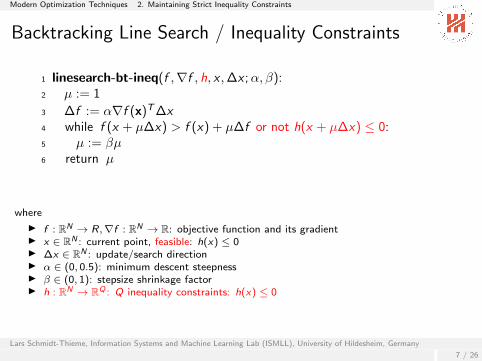
Backtracking Line Search / Inequality Constraints

1 linesearch-bt-ineq(f ,∇f , h, x ,∆x ;α, β):2 µ := 1

3 ∆f := α∇f (x)T∆x4 while f (x + µ∆x) > f (x) + µ∆f or not h(x + µ∆x) ≤ 0:5 µ := βµ6 return µ

where

I f : RN → R,∇f : RN → R: objective function and its gradientI x ∈ RN : current point, feasible: h(x) ≤ 0I ∆x ∈ RN : update/search directionI α ∈ (0, 0.5): minimum descent steepnessI β ∈ (0, 1): stepsize shrinkage factorI h : RN → RQ : Q inequality constraints: h(x) ≤ 0


7 / 26


Backtracking Line Search / Affine Inequality ConstraintsFor affine inequality constraints

h(x) = Bx − b ≤ 0

feasibility of an update can be guaranteed by a maximal stepsize:

h(x + µ∆x) =

B(x + µ∆x)− b ≤ 0

µB∆x ≤ −(Bx − b)

µ(B∆x)q ≤ −(Bx − b)q ∀q ∈ {1, . . . ,Q}

µ ≤ −(Bx − b)q(B∆x)q

∀q ∈ {1, . . . ,Q} : (B∆x)q > 0

µ ≤ min{−(Bx − b)q(B∆x)q

| q ∈ {1, . . . ,Q} : (B∆x)q > 0}

=: µmax


8 / 26


Backtracking Line Search / Affine Inequality Constraints

1 linesearch-bt-affineq(f ,∇f ,B, b, x ,∆x ;α, β):

2 µ := min{−(Bx−b)q(B∆x)q

| q ∈ {1, . . . ,Q} : (B∆x)q > 0}3 ∆f := α∇f (x)T∆x4 while f (x + µ∆x) > f (x) + µ∆f :5 µ := βµ6 return µ

where

I f : RN → R,∇f : RN → R: objective function and its gradientI x ∈ RN : current point, feasible: Bx − b ≤ 0I ∆x ∈ RN : update/search directionI α ∈ (0, 0.5): minimum descent steepnessI β ∈ (0, 1): stepsize shrinkage factorI B ∈ RQ×N , b ∈ RQ : Q affine inequality constraints: Bx − b ≤ 0


9 / 26

Modern Optimization Techniques 3. Gradient Projection Method for Affine Equality Constraints

Outline







10 / 26


Right Inverse Matrix

For A ∈ RN×M (N ≤ M) with full rank,the right inverse of A is

A−1right = AT (AAT )−1

Proof:

AA−1right = AAT (AAT )−1 = I


10 / 26


Nullspace Projection

For A ∈ RN×M (N ≤ M) with full rank, the matrix

F := I − A−1rightA = I − AT (AAT )−1A

is a projection onto the nullspace of A:

{x ∈ RM | Ax = 0} = {Fx ′ | x ′ ∈ RM}

Proof:

“ ⊇ ” : AFx ′ = A(I − A−1rightA)x ′ = (A− A)x ′ = 0

“ ⊆ ” : show: for any x with Ax = 0, there exists x ′ : x = Fx ′

x ′ := x : Fx ′ = Fx = (I − AT (AAT )−1A)x = x − AT (AAT )−1Ax= x − 0 = x


11 / 26


Gradient Projection Method / Affine Equality Constraints

1 min-gp-affeq(f ,∇f ,A, x (0), µ, ε,K ):

2 F := I − AT (AAT )−1A3 for k := 1, . . . ,K :

4 ∆x (k−1) := −FT∇f (x (k−1))

5 if ||∆x (k−1)|| < ε:

6 return x (k−1)

7 µ(k−1) := µ(f , x (k−1),∆x (k−1))

8 x (k) := x (k−1) + µ(k−1)∆x (k−1)

9 return ”not converged”

where

I A ∈ RP×N , a ∈ RP : P affine equality constraintsI x(0) feasible starting point, i.e., Ax(0) − a = 0


12 / 26


Grad. Proj. Meth. / Aff. Eq. Cstr. + strict In.eq. Constr

1 min-gp-affeq-strictineq(f ,∇f ,A, h, x (0), µ, ε,K ):

2 F := I − AT (AAT )−1A3 for k := 1, . . . ,K :

4 ∆x (k−1) := −FT∇f (x (k−1))

5 if ||∆x (k−1)|| < ε:

6 return x (k−1)

7 µ(k−1) := µ(f , h, x (k−1),∆x (k−1))

8 x (k) := x (k−1) + µ(k−1)∆x (k−1)

9 if ∃q ∈ {1, . . . ,Q} : hq(x (k)) = 0 :

10 return x (k)


where

I A ∈ RP×N , a ∈ RP : P affine equality constraintsI x(0) strictly feasible starting point, i.e., h(x(0))<0, Ax(0) − a = 0I µ(. . . , h, . . .) stepsize controller that retains inequality constraints hI h : RN → RQ : Q inequality constraints: h(x) ≤ 0


13 / 26

Modern Optimization Techniques 4. Active Set Methods: General Strategy

Outline







14 / 26


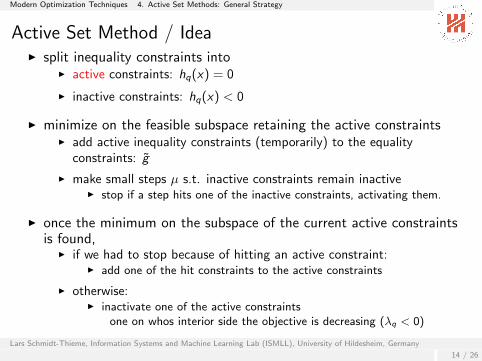
Active Set Method / IdeaI split inequality constraints into

I active constraints: hq(x) = 0

I inactive constraints: hq(x) < 0

I minimize on the feasible subspace retaining the active constraintsI add active inequality constraints (temporarily) to the equality

constraints: g

I make small steps µ s.t. inactive constraints remain inactiveI stop if a step hits one of the inactive constraints, activating them.

I once the minimum on the subspace of the current active constraintsis found,

I if we had to stop because of hitting an active constraint:I add one of the hit constraints to the active constraints

I otherwise:I inactivate one of the active constraints

one on whos interior side the objective is decreasing (λq < 0)


14 / 26


Active Set Methods / General Strategy1 min-activeset(f , g, h, x(0),K ,min-eq):

2 Q := {q ∈ {1, . . . ,Q} | hq(x(0)) = 0}

3 g :=

(ghQ

), h := h{1,...,Q}\Q

4 for k := 1, . . . ,K :

5 x(k) := min-eq(f , g, h, x(k−1))6 if ∃q ∈ {1, . . . ,Q} \ Q : hq(x) = 0:7 Q := Q ∪ {q} for an arbitrary q ∈ {1, . . . ,Q} \ Q with hq(x) = 0

8 g :=

(ghQ

), h := h{1,...,Q}\Q

9 else :10 if |Q| = 0:

11 return x(k)

12 compute Lagrange multipliers λq for hq , q ∈ Q13 if λ ≥ 0:

14 return x(k)

15 Q := Q \ {q} for an arbitrary q ∈ Q with λq < 0

16 g :=

(ghQ

), h := h{1,...,Q}\Q


whereI g : RN → RP : P equality constraints: g(x) = 0I h : RN → RQ : Q inequality constraints: h(x) ≤ 0I x(0) feasible starting point, i.e., g(x) = 0, h(x) ≤ 0I min-eq: solver for equality constraints and strict inequality constraints, e.g.,

min-gp-affeq-strictineq,Lars Schmidt-Thieme, Information Systems and Machine Learning Lab (ISMLL), University of Hildesheim, Germany

15 / 26


Computing the Lagrange Multipliers (line 12)

complementary slackness:

λqhq(x) = 0 λq = 0 ∀q 6∈ Qstationarity:

∇f (x) +P∑

p=1

νp∇gp(x) +Q∑

q=1

λq∇hq(x) = ∇f (x) +P∑

p=1

νp∇gp(x) = 0

solve LSE

(∇g1(x), . . . ,∇gP(x))

ν1...νP

= −∇f (x)

λq := νp for p ∈ {1, . . . , P} : gp = hq, q ∈ Q


16 / 26


Active Set Method / Remarks

I Limitation: To work with non-linear inequality constraints hq, theactive set method requires an equality-constrained optimizer min-eqthat can cope with non-linear equality constraints.

I because active inequality constraints hq are used as equality constraintsgp.

I The active set method can be accelerated by solving the equalityconstrained problem only approximately: ε

I but for the risk of zigzagging

book2008/10/23page 570�

��

�

��

��

570 Chapter 15. Feasible-Point Methods

x 0

x1

x 2

x 3

Figure 15.3. Zigzagging.

implementation, however. The reason is that as the solution to a problem becomes lessaccurate, the computed Lagrange multipliers also become less accurate. These inaccuraciescan affect the sign of a computed Lagrange multiplier. Consequently, a constraint mayerroneously be deleted from the working set, thereby wiping out any potential savings.

Another possible danger is zigzagging. This phenomenon can occur if the iterates cy-cle repeatedly between two working sets. This situation is depicted in Figure 15.3. Zigzag-ging cannot occur if the equality-constrained problems are solved sufficiently accuratelybefore constraints are dropped from the working set.

To conclude, we indicate how the active-set method can be adapted to solve a problemof the form

minimize f (x)

subject to A1x ≥ b1

A2x = b2

containing a mix of equality and inequality constraints. In this case, the equality constraintsare kept permanently in the working set W since they must be kept satisfied at every iteration.The Lagrange multipliers for equality constraints can be positive or negative, and so do notplay a role in the optimality test. The equality constraints also do not play a role in theselection of the maximum allowable step length α. These are the only changes that need bemade to the active-set method.

15.4.1 Linear Programming

The simplex method for linear programming is a special case of an active-set method.16

Suppose that we were trying to solve a linear program with n variables and m linearlyindependent equality constraints:

minimize f (x) = cTx

subject to Ax = b

x ≥ 0.

16This section uses the notation of Chapters 4 and 5.

[Griva et al., 2009, p.570]


17 / 26


ConvergenceTheorem (Active Set Theorem)If for every subset Q of inequality constraints the problem

arg minx∈RN

f (x)

subject to Ax − a = 0

BQx − bQ = 0

BQx − bQ < 0, Q := {1, . . . ,Q} \ Q

is well-defined with a unique nondegenerate solution (i.e.,λq 6= 0 ∀q ∈ Q), thenthe active set method converges to the solution of the inequality constrainedproblem.

Proof:

I After the minimum over the subspace defined by an active set has been found,I the function value further decreases when removing a constraint.I Thus the algorithm cannot possibly return to the same active set.I As there are only finite many possible active sets, it eventually will terminate.


18 / 26

Modern Optimization Techniques 5. Gradient Projection Method for Affine Inequality Constraints

Outline







19 / 26


Gradient Projection / Idea

I Gradient Projection:I use the active set strategy for Gradient Descent

(to solve the equality constrained subproblems)

I putting everything togetherI esp. for affine constraints


19 / 26


Gradient Projection / IdeaI split inequality constraints into

I active constraints: (Bx − b)q = 0

I inactive constraints: (Bx − b)q < 0

I find an update direction ∆x that retains this state of the inequalityconstraints

I add active inequality constraints (temporarily) to the equalityconstraints: A, a

I make small steps µ s.t. inactive constraints remain inactive:

(B(x + µ∆x)− b)q ≤ 0 µ ≤ −(Bx − b)q(B∆x)q

, for (B∆x)q > 0

I x + µ∆x may hit one of the inactive constraints, activating them.

I once the minimum on the subspace of the current active constraintsis found,

I inactivate one of the active constraintsI one on whos interior side the objective is decreasing (λq < 0)


20 / 26


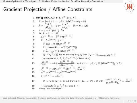
Gradient Projection / Affine Constraints

1 min-gp-aff(f , A, a, B, b, x(0), µ, ε,K):

2 Q := {q ∈ {1, . . . ,Q} | (Bx(0) − b)q = 0}

3 A :=

(A

BQ

), a :=

(a

bQ

), P := P + |Q|

4 F := I − AT (AAT )−1A5 for k := 1, . . . ,K :

6 ∆x(k−1) := −FT∇f (x(k−1))

7 if ||∆x(k−1)|| ≤ ε:

8 if |Q| = 0: return x(k−1)

9 λ := solve(Aλ = −∇f (x(k−1)))

10 if λP+1:P

≥ 0: return x(k−1)

11 Q := Q \ {q} for an arbitrary q ∈ Q with λq := λP+index(q,Q) < 0

12 recompute A, a, P, F ,∆x(k−1) (= lines 3,4,6)

13 µ(k−1)max := min{−(Bx(k−1)−b)q

(B∆x(k−1))q| q ∈ {1, . . . ,Q} \ Q, (B∆x(k−1))q > 0}

14 µ(k−1) := µ(f , x(k−1),∆x(k−1), µ(k−1)max )

15 x(k) := x(k−1) + µ(k−1)∆x(k−1)

16 if µ(k−1) = µ(k−1)max :

17 Q := Q ∪ {q} for an arbitrary q ∈ {1, . . . ,Q} \ Q with−(Bx(k−1)−b)q

(B∆x(k−1))q= µ

(k−1)max

18 recompute A, a, P, F (= lines 3−4)19 return ”not converged”


21 / 26


Gradient Projection / Affine Constraints (ctd.)

where

I A ∈ RP×N , a ∈ RP : P affine equality constraintsI B ∈ RQ×N , b ∈ RQ : Q affine inequality constraintsI x(0) feasible starting pointI µ(. . . , µmax) step length controller, yielding steplength ≤ µmaxI index(q,Q) := i for q = qi and Q = (q1, q2, . . . , qQ)


22 / 26


Remarks

I The projection matrix F does not have to be computed from scratch,every time the active constraint set changes, but can be efficientlyupdated.


23 / 26


Convergence / Rate of Convergence

I For the gradient projection method, a rate of convergence can beestablished.

I But the proof is somewhat involved(see [Luenberger and Ye, 2008, ch. 12.5]).


24 / 26


Summary

I Primal methods optimizeI in the original variables,

I staying always within the feasible area.

I Backtracking line search can be modified to retain strict inequalityconstraints.

I for affine inequality constraints: guaranteed by a maximum stepsize.

I The gradient projection method for affine equality constraints is amodified gradient descent.

I simply project gradients to the nullspace of the affine constraints.


25 / 26


Summary (2/2)

I Active set methodsI partition the inequality constraints into active and inactive ones

I an inequality constraint hq is active iff hq(x) = 0.

I add active inequality constraints temporarily to the equality constraints

I and solve this problem using an optimization method for equalityconstraints.

I break away from a random active inequality constraint into whosinterior of the feasible area the objective decreases.

I The gradient projection method (for affine equality and inequalityconstraints) is an active set method that uses the gradient projectionmethod for equality constraints to solve the equality constrainedsubproblems.


26 / 26


Further Readings

I Primal methods for constrained optimization are not covered by Boydand Vandenberghe [2004].

I Primal methods often also are called feasible point methods.

I Active set methods:I general idea: [Luenberger and Ye, 2008, ch. 12.3]

I Gradient projection method: [Luenberger and Ye, 2008, ch. 12.4+5],[Griva et al., 2009, ch. 15.4]

I Reduced gradient method: [Luenberger and Ye, 2008, ch. 12.6+7],[Griva et al., 2009, ch. 15.6]

I Further primal methods not covered here:I Frank-Wolfe algorithm / conditional gradient method: [Luenberger and

Ye, 2008, ch. 12.1]


27 / 26


References

Stephen Boyd and Lieven Vandenberghe. Convex Optimization. Cambridge University Press, 2004.

Igor Griva, Stephen G. Nash, and Ariela Sofer. Linear and Nonlinear Optimization. Society for Industrial and AppliedMathematics, 2009.

David G. Luenberger and Yinyu Ye. Linear and Nonlinear Programming. Springer, 2008.


28 / 26

modern optimization techniques...modern optimization techniques 1. inequality constrained...

Documents