modern forecasting models in action: improving ... · pdf filemodern forecasting models in...

Modern Forecasting Models in Action:Improving Macroeconomic Analyses at

Central Banks∗

Malin Adolfson,a Michael K. Andersson,a Jesper Linde,a,b

Mattias Villani,a,c and Anders Vredina

aSveriges RiksbankbCEPR

cStockholm University

There are many indications that formal methods are notused to their full potential by central banks today. In thispaper, using data from Sweden, we demonstrate how BVARand DSGE models can be used to shed light on questions thatpolicymakers deal with in practice. We compare the forecastperformance of BVAR and DSGE models with the Riksbank’sofficial, more subjective forecasts, both in terms of actual fore-casts and root mean-squared errors. We also discuss how tocombine model- and judgment-based forecasts, and show thatthe combined forecast performs well out of sample. In addi-tion, we show the advantages of structural analysis and use themodels for interpreting the recent development of the inflationrate through historical decompositions. Last, we discuss themonetary transmission mechanism in the models by comparingimpulse-response functions.

JEL Codes: E52, E37, E47.

∗We are grateful to Jan Alsterlind for providing the implicit-forward-ratedata, to Josef Svensson for providing real-time data on GDP, and to Mari-anne Nessen, Jon Faust, Eric Leeper, and participants in the “Macroeconomicsand Reality—25 Years Later” conference in Barcelona in April 2005, for com-ments on an earlier version of this paper. The views expressed in this paper aresolely the responsibility of the authors and should not be interpreted as reflectingthe views of the Executive Board of Sveriges Riksbank. Address for correspon-dence: Anders Vredin, Sveriges Riksbank, SE-103 37 Stockholm, Sweden. E-mail:[email protected].

111

112 International Journal of Central Banking December 2007

1. Introduction

Over the last two decades, there has been a growing interest amongmacroeconomic researchers in developing new tools for quantitativemonetary policy analysis. In this paper, we examine how the newgeneration of formal models can be used in the policy process atan inflation-targeting central bank. We compare official forecastspublished by Sveriges Riksbank (the central bank of Sweden) withforecasts from two structural models—a dynamic stochastic generalequilibrium (DSGE) model and an identified vector autoregression(VAR) estimated with Bayesian methods. We also discuss how theformal models can be used for storytelling and for the analysis ofalternative policy scenarios, which is an important matter for centralbanks.

It is rather unusual that formal models are contrasted to offi-cial central bank forecasts. Such a comparison is especially interest-ing given that the latter also include judgments and “extra-model”information, which are very hard to capture within a formal setting.Hence, this can give an assessment of how useful expert knowledgeis and shed light on the “role of subjective forecasting” raised bySims (2002). An evaluation of official forecasts and formal modelforecasts has, to our knowledge, only been conducted for the Boardof Governors of the Federal Reserve System (see Altig, Carlstrom,and Lansing 1995 and Sims 2002).1 We will supplement this analysisby evaluating official and model forecasts for a small open economy(Sweden).

Smets and Wouters (2004) have shown that modern closed-economy DSGEs (with various nominal and real frictions) haveforecasting properties well in line with more empirically orientedmodels such as standard and Bayesian VARs (BVARs). However,this paper evaluates forecasts from DSGE and BVAR models thatinclude open-economy aspects and compares these with judgmentalforecasts. Given the increased complexity of open-economy models,and the different monetary policy transmission mechanism whereexchange rate movements are of importance, our exercise adds an

1Before this paper was completed, Edge, Kiley, and Laforte (2006) comparedthe forecasting performance of the Federal Reserve with a closed-economy DSGEas well as with a theoretical reduced-form model.

Vol. 3 No. 4 Modern Forecasting Models in Action 113

extra element to the analysis in, e.g., Sims (2002) and Smets andWouters (2004). In section 2, we show the actual inflation and inter-est rate forecasts from the various setups as well as the root mean-squared errors (RMSEs) of the forecasts. In addition, we explicitlyexamine two episodes where official and DSGE forecasts diverge tolook further into the role of subjective forecasting.

Both the DSGE and BVAR models have now been used withinthe policy process at Sveriges Riksbank between one and two years.However, this does not provide us with enough observations to carryout an extensive forecast evaluation in genuine real time. Since theDSGE model uses data on as many as fifteen macroeconomic vari-ables, we have therefore estimated the formal models using a reviseddata set, which makes a much longer evaluation period of the variousforecasting methods possible. We discuss the role of real-time versusrevised data in detail in section 2 below.

In addition, we demonstrate how formal models can shed lighton practical policy questions. In section 3.1, we let the two modelsinterpret the underlying reasons for the recent economic develop-ment, using a historical decomposition of the forecast errors in eachof the two models. We also show that a VAR model can be usedto clarify what has happened in the economy, as long as we arewilling to impose some structure to identify the underlying shocks.However, when one is interested in predictions conditioned uponalternative policy scenarios, an idea about how monetary policyis designed and how it affects the economy is required. By com-paring impulse-response functions in section 3.2, we show that theDSGE model, using structure from economic theory, provides a muchmore reasonable transmission mechanism of monetary policy thanthe BVAR model. This is a necessary requirement for producingconditional forecasts that are meaningful from the perspective of acentral banker.

Finally, section 4 summarizes our views on the advantages of for-mal methods and the reasons why such methods have not been moreinfluential at central banks.

2. Forecasting Performance

This section provides an evaluation of the inflation, interest rate,and GDP forecasts by the Riksbank, a small-open-economy DSGE


model, and a Bayesian VAR model. Both actual forecasts androot mean-squared errors are examined for the period 1999:Q1–2005:Q4.2 To characterize the forecasting advantage of the Riks-bank’s judgmental forecasts, we also analyze two specific episodeswhere the different forecasting approaches diverge for CPI infla-tion and where we, a priori, expect the sector experts to havean informational advantage. Since the Riksbank’s forecasts haveuntil recently been intended to be conditioned on the assump-tion of a constant short-term interest rate, we also look at theinterest rate forecasts from the formal models.3 These are com-pared with implicit-interest-rate forecasts calculated from (market-based) forward interest rates. Finally, we also look at the GDPforecasts from the different models, but since no genuine real-time data set has been compiled for all fifteen variables in theDSGE model, these results should be interpreted with somecaution.4

2Official inflation forecasts from the Riksbank cannot be obtained on aquarterly basis before 1999:Q1. Moreover, the DSGE model needs a sufficientnumber of observations after the transition from a fixed exchange rate to theinflation-targeting regime in 1993. Since GDP forecasts are not available fromthe Riksbank before 2000:Q1, their precision is evaluated between 2000:Q1 and2005:Q4.

3Between October 2005 and February 2007, the Riksbank produced fore-casts conditioned upon implicit forward rates, instead of the constant-interest-rate assumption. Since February 2007, the Riksbank has published its preferredpath for the future repo rate (i.e., the short-term interest rate controlled by theRiksbank).

4The absence of a real-time data set implies that the formal models possiblyhave an information advantage relative to the official forecasts since the BVARand DSGE forecasts are based on ex post data on GDP. (Preliminary GDPdata are available with a delay of around one quarter, but they are subsequentlyrevised.) This is not a problem with the other variables in the models, since dataon prices, interest rates, and exchange rates are available on a monthly basis andare not revised. On the other hand, the official forecasts have a small informa-tion advantage in some quarters, when the Inflation Report has been publishedtoward the end of the quarter and, thus, can be based on data on prices, interestrates, and exchange rates from the early part of the same quarter. Since most ofthe variables in the BVAR are available in real time, and we use a Litterman (i.e.,random-walk) prior for the lag polynomial, there are good reasons to believe thatthe BVAR results with the exception of GDP growth are not very sensitive toour decision to use revised data. The DSGE model, which is estimated on a dataset that contains several additional real quantities, is probably more sensitive tothe use of revised data.


The Riksbank publishes official forecasts in its quarterly Infla-tion Report publication. The forecasts are not the outcome of asingle formal model but rather the result of a complex procedurewith input both from many different kinds of models and judgmentsfrom sector experts and the Riksbank’s executive board.5

The BVAR model contains quarterly data for the following sevenvariables: trade-weighted measures of foreign GDP growth in logs(yf ), CPI inflation (πf ) and a short-term interest rate (if ), the cor-responding domestic variables (y, π, and i), and the level of thereal exchange rate defined as q = 100(s + pf − p), where pf andp are the foreign and domestic CPI levels (in logs) and s is the (log)trade-weighted nominal exchange rate. More details on the BVARare provided in appendix 1.

The DSGE model is an extension of the closed-economy modelsdeveloped by Altig et al. (2003) and Christiano, Eichenbaum, andEvans (2005) to the small-open-economy setting in a way similar tothat of Smets and Wouters (2002). Households consume and investin baskets consisting of domestically produced goods and importedgoods. We allow the imported goods to enter both aggregate con-sumption and aggregate investment. By including nominal rigidi-ties in the importing and exporting sectors, we allow for short-runincomplete exchange rate pass-through to both import and exportprices. The foreign economy is exogenously given by a VAR forforeign inflation, output, and the interest rate. The DSGE modelis estimated with Bayesian methods using data on the followingfifteen variables: GDP deflator inflation, real wage, consumption,investment, real exchange rate, short-run interest rate (repo rate),hours, GDP, exports, imports, CPI inflation, investment deflatorinflation, foreign (i.e., trade-weighted) output, foreign inflation, andforeign interest rate. The DSGE model is identical to the one devel-oped and estimated by Adolfson et al. (forthcoming), and a more

5The forecast process during the evaluation period was of a recursive and iter-ative nature, where the foreign and financial variables entered first. Given theseforecasts, the Swedish real variables were predicted. Typically, the GDP forecastwas an aggregation of the components of the GDP identity. The labor-marketvariables entered in a third step, where the productivity and unit-labor-cost vari-ables were determined. Finally, predictions of CPI and core inflation—mainlybased on forecasts of import prices, unit labor cost, and the output gap—endedthe first forecast round.


detailed description of the model, priors used in the estimation, andfull-sample estimation results can be found in that paper.

The DSGE model contains more variables than the BVAR, butthis does not imply that the DSGE model necessarily has an advan-tage in terms of the forecasting performance, since the inclusion ofmore variables in the BVAR also implies that a considerably largernumber of parameters needs to be estimated. Adolfson et al. (forth-coming) consider a BVAR with the same set of variables as in theDSGE model, and the forecasting performance of this BVAR is notvery different from the BVAR used in this paper.6

One difficulty when it comes to comparing official inflation fore-casts from the Riksbank with model forecasts (or forecasts madeby other institutions) is that the Riksbank’s forecasts have untilrecently been intended to be conditioned on the assumption thatthe short-term interest rate (more specifically, the Riksbank’s instru-ment, the repo rate) remains constant throughout the forecastingperiod. However, it is not unreasonable to assume that the officialforecast actually lies closer to an unconditional forecast, given itssubjective nature. In practice, it is extremely difficult to ensure thatthe judgmental forecast has been conditioned on a constant-interest-rate path rather than on some more likely path.7 Beyond the forecasthorizon, the implicit assumption also seems to have been that theinterest rate gradually returns to a level determined by some inter-est rate equation. Even so, we see from figure 1 (shown on the nextset of facing pages) that the interest rate level (annualized aver-age of daily repo-rate observations within each quarter) has beenrather stable during the sample period, which is the reason why a

6If anything, the introduction of additional variables leads to a reduction inforecasting performance. In particular, this appears to be the case for the nominalinterest rate.

7The Inflation Reports from March and June 2005 contain discussions of theproblems with constant-interest-rate forecasts, as well as two forecasts of inflationand GDP growth that are conditional on either a constant interest rate or theimplied forward rate. Although there was a considerable difference between theforward rate and the constant interest rate on these occasions (a gradual increaseto about 150 basis points at the two-year horizon), the forecasts for GDP andinflation were not very different. This suggests that the official constant-interest-rate forecasts were in fact close to unconditional projections. See also Adolfsonet al. (2005) for difficulties with constant-interest-rate forecasts in a model-basedenvironment.


conceivable constant-interest-rate assumption might not have beenthat unfavorable. Moreover, the impulse-response functions frominterest rate changes to inflation are typically fairly small, with asubstantial time delay, at least in the BVAR model (see figure 6 insection 3.2), which implies that a constant-interest-rate assumptionat long horizons should have relatively small effects on the infla-tion forecast. We therefore believe that, taken together, our forecastcomparisons are valid and our conclusions will not be significantlyaffected by the alleged constant-interest-rate assumption underlyingthe official forecasts.

2.1 Inflation Forecasts

Figure 1a presents the outcome of CPI inflation in Sweden for 1998–2005 (bold line) together with the Riksbank’s official forecasts (firstrow), the forecasts from the DSGE model (second row), and theBVAR model (third row) for 1999:Q1–2005:Q4.8 The visual impres-sion is that the official forecasts and the model forecasts have some-what different properties. The Riksbank’s forecasts appear to berather “conservative”; most often they predict a very smooth devel-opment of inflation, and the changes in the forecast paths are rela-tively small between quarters. The BVAR model, on the other hand,seems to view the inflation process as more persistent, since forecasterrors have a larger influence on subsequent forecasts.

The top panel in figure 2 shows the root mean-squared errors(RMSEs) for different forecast horizons (one to eight quarters ahead)of the yearly CPI-inflation forecasts. The DSGE and the official fore-casts have about the same precision for inflation forecasts made upto a year ahead; however, at somewhat longer horizons (five to eightquarters ahead), the forecasts from the DSGE model have a bet-ter accuracy than the official inflation forecasts. The BVAR fore-casts, on the other hand, perform very well up to six quarters aheadbut are beaten by the DSGE’s inflation forecasts at longer hori-zons. It should also be noted that all three forecasting methods are

8The data in figure 1 refer to yearly inflation rates (pt − pt−4), just like theinflation series published in the Inflation Report. Since the DSGE and BVARmodels are specified in terms of quarterly rates of change (pt − pt−1), the modelforecasts are summed up to fourth differences.


Figure 1a. Sequential Forecasts of Yearly CPI Inflation,1999:Q1–2005:Q4, from the Riksbank (First Row),

the DSGE Model (Second Row), and theBVAR Model (Third Row)


Figure 1b. Sequential Forecasts of Repo Rate,1999:Q1–2005:Q4, from the Riksbank (First Row),



Figure 1c. Sequential Forecasts of Yearly GDP Growth,1999:Q1–2005:Q4, from the Riksbank (First Row),



Figure 2. Root Mean-Squared Error (RMSE) of YearlyCPI-Inflation Forecasts (Top) and Annualized InterestRate Forecasts (Middle) 1999:Q1–2005:Q4, and YearlyGDP-Growth Forecasts (Bottom) 2000:Q1–2005:Q4


better than a naive forecast of constant yearly inflation (the NoChange—Yearly line). We take the similar precision in the differ-ent inflation forecasts as evidence in favor of all three forecastingapproaches. It is encouraging that the model forecasts are perform-ing as well as the official forecasts also at shorter horizons. We will,however, return to the specific advantages and the role of subjectiveforecasting below.

Although Smets and Wouters (2004) have shown that the fore-casting performance of closed-economy DSGE models comparesquite favorably to more empirically oriented models such as vec-tor autoregressive models, it is not evident that our DSGE modelwill have similar properties, given that the open-economy dimen-sions add complexity to the model. In particular, it is well knownthat uncovered interest rate parity (UIP) is rejected empirically,which may deteriorate the forecasting performance of an open-economy DSGE model. The UIP condition in the DSGE model hastherefore been modified to allow for a negative correlation betweenthe risk premium and expected exchange rate changes; see Adolf-son et al. (forthcoming) for further details. Figure 2 reveals thatour DSGE model has a forecasting performance for CPI inflationthat is remarkably good. The DSGE model makes smaller fore-cast errors for inflation six to eight quarters ahead than both theBVAR and the official Riksbank forecasts. Part of this can beattributed to the modified UIP condition (see Adolfson et al. forth-coming), but we also believe that the fact that we are consider-ing a stable regime with a known and fixed inflation target makesthe theoretical structure imposed by the DSGE model particularlyuseful.

2.2 Interest Rate Forecasts

Figure 1b shows outcomes of the repo rate along with either theexpected interest rate paths derived from forward interest rates (firstrow), following the method described by Svensson (1995), or alongwith the repo-rate forecasts from the DSGE model (second row)and the BVAR model (third row). Throughout our sample, forwardinterest rates have systematically overestimated the future interestrate level. In principle, this could be due to (possibly time-varying)


term and risk premia; i.e., forward rates do not provide direct esti-mates of expectations. But, in practice, we believe it to be morelikely that the market (along with the Riksbank and the DSGEmodel) on average overestimated the inflation pressure and the needfor higher nominal interest rates during this period. Turning to theinterest rate forecasts from the formal models, we see that futureinterest rates have been systematically overestimated also in thiscase, even if the BVAR forecasts have been more moderate thanthe interest rate forecasts from the DSGE model. The main reasonfor the relatively large forecast errors of the DSGE model for therepo rate is that the model has tended to overestimate both theinflation pressure and the GDP-growth prospects during the period,which can be seen in figures 1a and 1c. This indicates that it is notthe estimated policy rule that does not fit the data: had we usedthe true inflation and output outcomes when projecting with therule, the forecast errors for the repo rate would have been greatlyreduced.

In the middle panel of figure 2, we compare the RMSEs forthe various repo-rate forecasts. It can be seen that forward inter-est rates, a naive constant-interest-rate forecast, and the BVARmodel all have about the same precision for forecasts three to fourquarters ahead, whereas the DSGE has somewhat worse accuracy.Naturally, this raises some questions about how monetary policy isdescribed in the DSGE model, although the above reasoning sug-gests that the policy rule itself may not be the key problem. For-ward rates have a better precision one to two quarters ahead, whilethe BVAR model makes much better forecasts for longer horizonsthan the other approaches. The fact that the BVAR model pro-vides a more realistic picture than forward rates at longer horizons,which even seem to have a lower predictive power than the constant-interest-rate assumption, may be interpreted as arguments againstinflation forecasts conditioned on forward rates. Nevertheless, thisis an assumption that the Bank of England recently adopted, andNorges Bank and Sveriges Riksbank recently abandoned. It shouldbe emphasized, however, that our results have been obtained froma sample where the short-term interest rate has been unusuallylow and stable in a historical context. Thus, it is possible thatforward rates are more informative in periods when interest rateschange more.


2.3 GDP Forecasts

Figure 1c shows the forecasts for the yearly GDP growth from theRiksbank, the DSGE, and the BVAR models against actual yearlyGDP growth (last data vintage in all cases). Given that the Riks-bank’s forecasts are made in real time, whereas the formal modelsare estimated using a revised data set for GDP, a direct comparisonbetween them is hard to make. The pattern between the DSGE andBVAR forecasts is relatively similar, however. This also shows upin the root mean-squared errors for the forecasts in figure 2. Themodels’ accuracy in terms of predicting GDP growth is almost thesame in this sample (2000:Q1–2005:Q4).

To increase the comparability of the forecasting performances,we compute the RMSEs for the Riksbank’s GDP forecasts in real-time data, since the formal models would have an informationaladvantage if all these GDP forecasts were evaluated on the reviseddata set. The models appear to perform reasonably well also againstthe judgmental forecasts of the Riksbank (see figure 2), although itshould be emphasized that such a comparison should be interpretedwith caution.

2.4 The Role of Subjective Forecasting

To obtain more information about the properties of the variousapproaches to forecasting, it is interesting to take a closer look atsome specific episodes where the pure model forecast and the officialRiksbank forecast differ. This provides us with useful informationabout whether sector experts can provide a better understanding ofrecent influences on inflation (which might only be temporary). Infigure 3, we compare the Riksbank’s official inflation forecasts withthe corresponding DSGE forecasts on four different occasions (i.e.,figure 3 contains a subset of the information in figure 1).9

The first episode concerns forecasts made immediately beforeand after the sudden increase in inflation in 2001:Q2. One importantfactor behind this increase was a rise in food prices due to the mad-cow and foot-and-mouth diseases, although the inflation rate had

9For ease of exposition, we only focus on the Riksbank and DSGE forecastshere.


Figure 3. Riksbank and DSGE Forecasts of YearlyCPI Inflation Made on Four Specific Occasions:

2000:Q4, 2001:Q2, 2003:Q1, and 2003:Q3

started to increase already in 1999. In 2000:Q4, the Riksbank’s offi-cial forecast implied a slowly increasing inflation rate over the nexttwo years. The DSGE model suggested a much stronger increasein inflation. This may reflect that the model forecast attributed alarger weight to recent increases in inflation, while the subjectiveprocedure, leading up to the Riksbank’s official forecast, underes-timated the persistence in changes in inflation. However, once theshock had become apparent, the subjective approach proved to bevery useful. At that time, 2001:Q2, the sector experts expectedthe food price increase to involve a persistent shock to the pricelevel but with small further effects on the yearly inflation rate, andthe Riksbank’s forecasts at 2001:Q2 were more in line with theactual outcome for the next few quarters. The DSGE model, onthe other hand, treated the food price shock as any other inflationshock and overestimated its effects on inflation during both 2001 and2002.

The second episode concerns inflation forecasts made in 2003:Q1.Cold, dry weather had brought about extreme increases in electric-ity prices during the winter of 2002/03. This was a temporary shock


to the price level, but it had persistent effects on yearly inflation,which became unusually low when electricity prices declined duringthe spring and summer. The Riksbank’s official forecasts describedthe decline in inflation extremely well for the first two quarters butunderestimated the effects on the longer horizons, possibly becauseit was difficult to separate the effects of changes in energy prices(the oil price also fluctuated heavily) from the downward pressureon inflation from other forces in the economy (e.g., increases in pro-ductivity). In contrast, the DSGE model underestimated the drop ininflation at first, but once the decline had started, it more correctlypredicted that inflation would be very low for the next one to twoyears (cf. the forecasts from 2003:Q3 in figure 3).

These episodes nicely illustrate how formal statistical mod-els and judgments by sector experts can complement each other.Subjective forecasts may sometimes be too myopic and pay too lit-tle attention to systematic inflation dynamics related to the businesscycle or other historically important regularities. Model forecasts,on the other hand, cannot take sufficient account of specific unusualbut observable events. At the same time, judgments from sectorexperts based on their detailed knowledge about the economy canbe extremely useful—in particular, when unusual shocks have hitthe economy.

2.5 Combined Forecasts

The previous subsections have contrasted model-based andjudgment-based macroeconomic forecasts, and have made it clearthat judgments from sector experts can be useful in the short run,especially when unusual disturbances to the economy occur. Beingequipped with several different forecasts, our natural question is,what can be gained from combining them into a single overall fore-cast? Combining a set of purely model-based forecasts is ratherstraightforward, especially within the Bayesian framework, wherethe weights are given by posterior model probabilities (Draper 1995).When at least one of the forecasting models cannot be representedby a probability model for the observed data, we need to resort toother solutions.

Winkler (1981) proposes an alternative Bayesian approach thatmay be used to combine model-based and judgment-based forecasts.


We will form weights separately for each variable and forecast hori-zon. Winkler’s procedure is described in detail in appendix 2. Themethod assumes that the forecast errors from the different fore-casts at a specific time period follow a multivariate normal dis-tribution with zero mean and covariance matrix Σ. It is furtherassumed that the forecast errors are independent over time. Theoptimal weights on the individual forecasts can then be shown tobe a simple function of Σ−1. This means that the weights dependnot only on the relative precision of the forecasts but also on thecorrelation between forecast errors. It should be noted that whilethe weights sum to unity, some weights may be negative. Neg-ative weights arise quite naturally, especially when the forecasterrors are highly correlated (Winkler 1981), but for conveniencein interpretation, we shall restrict all weights to be non-negative.The results do not change substantially if we allow for negativeweights.

The forecast-error covariance matrix Σ needs to be estimatedfrom the realized forecast errors available at the time of the for-mation of the combined forecast. This means that Σ needs to beestimated from a small number of observations. We use a prior dis-tribution to stabilize the estimate of Σ (see appendix 2 for details).Before turning to the results, it should be noted that we have notconducted this weighting experiment for GDP due to the real-timeproblems related to this variable.

The assumption of unbiased forecast errors does not seem tohold for the DSGE and implicit-forward-rate forecasts of the inter-est rate (see figure 7 in appendix 2), which may have consequencesfor the combined forecasts. However, the combined forecast withweights inversely related to the univariate mean-squared forecasterrors (MSEs), which thus include any potential bias, yields similarresults in terms of its accuracy (see figure 2).

From figure 2, we also see that the combined CPI-inflationforecast performs very well at all forecast horizons. The excellentperformance of the combined forecast at the first-quarter horizonis particularly noteworthy. We want to stress that we only usethose forecast errors that were actually available at the time of theforecast. This means that the RMSE evaluation at, e.g., the eight-quarter horizon only uses weights up to 2003:Q4 (the sample endsin 2005:Q4).


Turning to the short-term interest rate, we see once more thatcombining forecasts is a good idea. The RMSE of the combinedforecast is low for all forecast horizons, only slightly beaten by theimplicit forward rate at the first two horizons and the BVAR forecastat the longer horizons (see the middle panel of figure 2).

3. Advantages of Structural Analysis

3.1 Historical Decompositions

In section 2, we analyzed the usefulness of DSGE and BVAR modelsfor forecasting purposes. But policymakers are also very interested inunderstanding the factors that have brought the economy to whereit is right now. This necessitates a structural model that can disen-tangle the underlying causes for the recent economic development.In the DSGE model, all shocks are given an economic interpreta-tion, while the BVAR model requires additional identifying restric-tions. As an example of the use of models for structural analysis,we let the two models interpret the low inflation rate in Swedenduring 2003–05, by decomposing the model projections into thevarious shocks that have driven the development of inflation andoutput.

In figure 4, we report the actual outcome of GDP growth, infla-tion, and the repo rate together with projections from the BVARmodel. The first row of figure 4 reports forecasts made in 2003:Q1under the assumption that no shocks would hit the Swedish econ-omy during 2003–05. It can be seen that parts of the increase inGDP growth and the decreases in inflation and the interest ratewere expected, but actual inflation turned out to be a great deallower than anticipated by the BVAR model. From the second rowof figure 4—where we have added the “foreign” shocks, identified bythe BVAR model ex post (dashed line), to the BVAR model’s no-shock (expected) scenario (dotted line)—we can see that the suddendrop in inflation during 2003 and the lower GDP growth during thefirst quarters of 2003 were mainly due to foreign shocks hitting theeconomy.10 The last row of figure 4 shows the effects of “domestic”

10The foreign shocks are identified through the assumption that foreignGDP growth, foreign inflation, and the foreign interest rate are strictly


Figure 4. Actual Outcomes (−−) and Predictions for2003:Q2–2005:Q4 from the BVAR Model without Any

Shocks (· · · ) and with Only Subsets of the Shocks Activeduring the Forecasting Period (−−−)

shocks, which are simply identified residually as the parts of the fore-cast errors that are not accounted for by foreign shocks. From thelast row, we see that with only domestic shocks, the BVAR modeloverestimates inflation during 2003, although overall macroeconomicgrowth seems to be well captured. For 2004 and 2005, the picture issomewhat different, and during these years it is clear from figure 4

exogenous. Formally, this implies, among other things, that the foreign variablesare ordered before all domestic variables in the Choleski decomposition. In addi-tion, the forecast-error decompositions in figure 4 are based on the assumptionthat the real exchange rate is ordered last in the Choleski decomposition. Theresults are not affected much, however, if we instead assume that real-exchange-rate shocks are treated as foreign. The results are available upon request. Noattempt is made to identify individual foreign shocks.


that the domestic shocks have been a more important source for theforecast errors in general and the low inflation rate in particular.In principle, it is also possible to get even more information aboutthe shocks from the BVAR model, as long as we are willing to makeadditional identifying assumptions.11

In figure 5, we instead decompose the forecast errors from theDSGE model. The first row shows the outcome of GDP growth, infla-tion, and the interest rate along with the predictions from the DSGEmodel under the assumption that no shocks are hitting the econ-omy (i.e., the corresponding information to the first row of figure 4,which was based on the BVAR model). Both models overestimatedinflation and the interest rate, but the DSGE model also overratedGDP growth to a somewhat larger extent. The other rows in figure 5show the “ex post forecasts” from the DSGE model when we addthe model’s estimates of different kinds of shocks during 2003–05(dashed lines) to the original forecasts from 2003:Q1 (dotted lines):monetary policy shocks (second row), technology shocks (third row),markup shocks (fourth row), foreign shocks (fifth row), preferenceshocks (sixth row), and fiscal policy shocks (last row). It can beseen that when the estimated technology shocks and foreign shocksare individually taken into account, the “ex post forecasts” of infla-tion from the DSGE model are rather close to the outcome. TheDSGE model thus supports the finding from the BVAR model thatmany of the forecast errors during 2003 were due to foreign shocks.In 2004 and 2005, when the BVAR model suggested that foreignshocks were less important, the DSGE model attributes a large partof the low inflation to both foreign shocks and domestic technologyshocks. Interestingly, the model suggests that increased competition(i.e., lower markups) is not an important factor for directly under-standing the low-inflation outcome. However, it is, of course, possiblethat the increased degree of openness (i.e., “globalization”) has stim-ulated the favorable development in total factor productivity. It isalso clear from figure 5 that fiscal policy shocks have played a very

11Other identifying restrictions may involve, e.g., restrictions on long-runimpulses as in King et al. (1991). Jacobson et al. (2001) present some resultsbased on such restrictions from a VAR model using similar data as this paper.Alternatively, restrictions may be imposed directly on the impulse-response func-tions as suggested by Canova and de Nicolo (2002) and Uhlig (2005).


Figure 5. Actual Values (−−) and Predictions for2003:Q2–2005:Q4 from the DSGE Model without

Any Shocks (· · · ) and with Only Subsets of the ShocksActive during the Forecasting Period (−−−)


limited role during this period and that monetary policy has, infact, been expansionary. According to the DSGE model, the Riks-bank reduced the repo rate more than the usual amount during thisperiod to prevent inflation from falling too far below the target.

We find the results from these exercises very promising. Notonly can the BVAR and DSGE models make forecasts that have,on average, an equal or better precision than the Riksbank’s official,more subjective forecasts, but they can also, ex post, decompose theforecast errors in ways that are informative for policymakers andadvisers.

3.2 The Effects of Monetary Policy Shocks

In the previous sections, we have shown that the BVAR model isa fine forecasting tool, but to some extent it can also explain whathas happened in the economy, as long as we are willing to placesome identifying assumptions on the shocks. However, to answerquestions about how monetary policy is designed and how it influ-ences the economy, we need to add further structure. Working withan identified model is especially important in a central bank envi-ronment where experiments such as predictions conditioned uponalternative interest rate paths are carried out. Therefore, we studyimpulse-response functions to see how the links between the interestrate setting and inflation outcomes differ between the BVAR andDSGE models.

Figure 6 displays the effects on output growth, CPI inflation,the repo rate, and the real exchange rate to a one-standard-deviationinterest rate shock in the BVAR model (first column) and the DSGEmodel (last column).12

Qualitatively, there are some similarities between the impulseresponses in the two models. For example, an increase in the inter-est rate appreciates the real exchange rate. However, there are also

12In the BVAR model, this is implemented through exogenous shocks to theinterest rate in a Choleski decomposition where the interest rate is ordered afterall other variables except the real exchange rate. Other nonrecursive identify-ing restrictions (e.g., allowing the central bank to react to changes in the realexchange rate within the period, but not to the two GDP variables) gave similarresults. In the DSGE model, exogenous shocks are added to the central bank’sreaction function (i.e., a monetary policy shock).


Figure 6. Posterior Median Impulse-Response Functionsto a One-Standard-Deviation Interest Rate Shock for the

Domestic Variables in the BVAR (First Column) andDSGE Model (Second Column) with 68 Percent and

95 Percent Probability Bands

discrepancies between the BVAR and the DSGE models. Althoughan increase in the interest rate causes a decline in output growthand inflation, consistent with typical prejudices, the responses in theBVAR are not significant in contrast to those in the DSGE model.Moreover, the DSGE model fulfills long-run nominal neutrality (i.e.,monetary policy can only affect prices and not real quantities in thelong run), whereas there is no such restriction in the BVAR. Fur-ther, the quantitative differences are very large. The DSGE modelsupports conventional wisdom: if the interest rate is unexpectedlyincreased by 0.35 percentage point (and then gradually reduced), themaximum effect on inflation is around 0.15 percentage point and is


recorded after about 1–112 years. The effects in the BVAR model are

much smaller and typically insignificant.Although there are reasons to expect that monetary policy shocks

are more credibly identified in the DSGE model, the differences inimpulse-response functions and forecasting properties between theBVAR and the DSGE models may create difficulties when using themodels in the policy process, even if each individual model com-pares well with the subjective forecasts and rests on solid method-ological grounds. Given the small impact of interest rate changesin the BVAR model, inflation projections conditional upon alter-native interest rate paths would not differ to any considerableextent from the BVAR’s unconditional forecasts. In contrast, theresults in figure 6 suggest that the DSGE’s conditional forecasts willchange a great deal compared with the unconditional forecasts if theformer are generated by injecting monetary policy shocks (whichhave much larger effects in the DSGE model). The impression ofalternative policy assumptions will thus be very different in thetwo models.

4. Concluding Remarks

The theme of this paper is that modern macroeconomic tools likeBVAR and DSGE models deserve to be used more in real-timeforecasting and for policy advice at central banks. We have shownthat it is possible to construct and use BVAR and DSGE modelsthat make about as good inflation forecasts as the much more com-plicated judgmental procedure typically employed by central banks.In our view, central banks should use formal models—VARs andDSGEs—as benchmarks for forecasts and policy advice, and to sum-marize the implications of the continuous flow of new informationabout the state of the economy to which central bank economistsare exposed.

We want to emphasize that we do not view our results as argu-ments against the use of judgments in monetary policy analysis.The key point here is not to dispute judgments versus formal mod-els but, rather, to determine how to coherently combine the BVARand DSGE models with beliefs about the current conditions. Ourresults suggest that it would be beneficial to incorporate judg-ments into the formal models, so that the forecasts reflect both


judgments and historical regularities in the data.13 We have ana-lyzed a Bayesian weighting scheme based on the forecast errors ofthe different methods to combine the judgmental and model fore-casts. The results are promising: the root mean-squared errors of thecombined forecasts of the CPI and the interest rate are consistentlylow on all evaluated forecast horizons. As an alternative, short-runjudgments by sector experts could be directly incorporated into themodels by exploiting the methodology suggested in Waggoner andZha (1999).

There are a number of gains in using formal models in the policyanalysis. They make it possible to decompose forecast errors and pro-vide a tool for characterizing the uncertainty involved in statementsabout the future development in the economy. Formal models makeit possible to quantify the imprecision and uncertainties involvedin the forecasting process. Formal models also serve as a learningmechanism, where lessons about the complex interdependencies inthe economy can be accumulated. Our results suggest, for example,that subjective forecasts may be too myopic and not take sufficientaccount of important historical regularities in the data. Our presentversion of the DSGE model, on the other hand, may reflect problemswith interest rate determination in financial markets, i.e., the empir-ical failure of the expectation hypothesis and the UIP condition; seethe discussion in, e.g., Faust (2005).

Naturally, there are also limitations to the use of the current gen-eration of modern macroeconomic models for policy purposes. Poli-cymakers are often interested in details about the state of the currenteconomy. Formal models cannot possibly cover all details within atractable consistent framework. Neither can sector experts, but theirinsights into details often lead policymakers to rely on advice andforecasts from experts rather than from models. Another problem isthat there are gaps between different models. Different models givequite different forecasts and imply different policy recommendations.Researchers are not typically bothered by this, as long as the mod-els are considered to be good. Policymakers are, of course, bothered.

13Svensson (2005) offers a theoretical analysis of the links between judgmentsand monetary policy. One way of including judgments in the formal models isto approach this in a Bayesian manner. However, it is less clear how to translatethe provided form of judgment into a usable prior distribution.


For some policy purposes, we therefore think that it makes sense toweight various models according to their empirical performance. Wehave discussed a procedure for combining forecasts that may also beused when some of the forecasts do not come from a well-specifiedformal model, which is typically the case in policy work. Anotherway of bridging the gap between formal models is to use Bayesianprior distributions that incorporate identical prior information onfeatures that are common to the models, such as the steady state ofthe system (Villani 2005) or impulse-response functions (Del Negroand Schorfheide 2004).

Appendix 1. The BVAR Model

The BVAR model contains quarterly data on the following sevenvariables: trade-weighted measures of foreign GDP growth (yf ), CPIinflation (πf ) and the three-month interest rate (if ), the correspond-ing domestic variables (y, π, and i, where i is the repo rate), and thelevel of the real exchange rate defined as q = 100(s + pf − p), wherepf and p are the foreign and domestic CPI levels (in logs) and s isthe (log of the) trade-weighted nominal exchange rate.

The BVAR model used in this paper is of the form

Π(L)(xt − Ψdt) = Aεt, (1)

where x = (yf , πf , if , y, π, r, q)′ is an n-dimensional vector of timeseries, Π(L) = In − Π1L − . . . − ΠkLk, and L is the usual back-shiftoperator with the property Lxt = xt−1. The structural distur-bances εt ∼ Nn(0, In), t = 1, . . . , T , are assumed to be indepen-dent across time. We impose restrictions on Π(L) such that theforeign economy is exogenous. A is the lower-triangular (Choleski)contemporaneous-impact matrix, such that the covariance matrixΣ of the reduced-form disturbances decomposes as Σ = AA′. Wealso have experimented with nonrecursive identifying restrictions,in which case the equations are normalized with the Waggoner-Zharule (Waggoner and Zha 2003b), and the Gibbs sampling algorithmin Waggoner and Zha (2003a) is used to sample from the posteriordistribution. The deterministic component is dt = (1, dMP,t)′, where

dMP,t ={

1 if t < 1993:Q10 if t ≥ 1993:Q1


is a shift dummy to model the abandonment of the fixed exchangerate and the introduction of an explicit inflation target in 1993:Q1.Since the data are modeled on a quarterly frequency, we use k = 4lags in the analysis. Larger lag lengths gave essentially the sameresults, with a slight increase in parameter uncertainty.

The somewhat nonstandard parameterization of the VAR modelin (1) is nonlinear in its parameters but has the advantage thatthe unconditional mean, or steady state, of the process is directlyspecified by Ψ as E0(xt) = Ψdt. This allows us to incorporate priorbeliefs directly on the steady state of the system, e.g., the informa-tion that steady-state inflation is likely to be close to the Riksbank’sinflation target. To formulate a prior on Ψ, note that the speci-fication of dt implies the following parameterization of the steadystate:

E0(xt) ={

ψ1 + ψ2 if t < 1993:Q1ψ1 if t ≥ 1993:Q1,

where ψi is the i-th column of Ψ. The elements in Ψ are assumed tobe independent and normally distributed a priori. The 95 percentprior probability intervals are given in table 1.

The prior proposed by Litterman (1986) will be used on thedynamic coefficients in Π, with the default values on the hyperpa-rameters in the priors suggested by Doan (1992): overall tightness isset to 0.2, cross-equation tightness to 0.5, and a harmonic lag decaywith a hyperparameter equal to 1. See Litterman (1986) and Doan(1992) for details. Litterman’s prior was designed for data in levelsand has the effect of shrinking the process toward the univariaterandom-walk model. Therefore, we set the prior mean on the firstown lag to 0 for all variables in growth rates. The two interest ratesand the real exchange rate are assigned a prior that centers on theAR(1) process with a dynamic coefficient equal to 0.9. The usual

Table 1. Ninety-Five Percent Prior ProbabilityIntervals of Ψ

yf πf rf y π r q

ψ1 (2, 3) (1.5, 2.5) (4.5, 5.5) (2, 2.5) (1.7, 2.3) (4, 4.5) (−1, 1)ψ2 (−1, 1) (1.5, 2.5) (1.5, 2.5) (−1, 1) (4.3, 5.7) (3, 5.5) (−9, 9)


random-walk prior is not used here, as it is inconsistent with havinga prior on the steady state. Finally, the usual non-informative prior|Σ|−(n+1)/2 is used for Σ.

The posterior distribution of the model’s parameters and theforecast distribution of the seven endogenous variables were com-puted numerically by sampling from the posterior distribution withthe Gibbs sampling algorithm in Villani (2005).

Appendix 2. Combining Judgmental and Model Forecasts

Suppose that we have available forecasts, at a given forecast hori-zon, from k different forecasting methods over T different timeperiods. Let xjt denote the j-th method’s forecast of a variablext, and ejt = xjt − xt the corresponding forecast error, wherej = 1, . . . , k and t = 1, . . . , T . The question here is how tomerge these k forecasts into a single combined forecast. FollowingWinkler (1981), we shall assume that the vector of forecast errorsfrom the k methods, et = (e1t, . . . , ekt)′, can be modeled as inde-pendent draws from a multivariate normal distribution with zeromean and covariance matrix Σ. This implies that xt ∼ Nk(xtu, Σ),where xt = (x1t, . . . , xkt)′ is the vector of forecasts of xt from thek forecasting methods, and u = (1, . . . , 1)′. We use an uninforma-tive (uniform) prior on xt and an inverted Wishart density for Σa priori: Σ ∼ IW (Σ0, v), where Σ0 = E(Σ) and v ≥ k is thedegrees-of-freedom parameter. The prior on Σ is important, as his-torical forecast errors are limited and an estimate of Σ is typicallyunreliable. This is particularly important when the correlations inΣ are large, which is often the case with forecast errors from com-peting methods. As v increases, the prior becomes increasingly con-centrated around Σ0. The specification of Σ0 and v is discussedbelow.

The posterior mean of the true value xt, which is the naturalcombined forecast for a Bayesian, can now be shown to be a linearcombination of the individual forecasts (Winkler 1981):

E(xt|xt) =k∑

j=1

wjtxjt, (2)


where the weights of the forecasting methods are given by

w′t = (w1t, . . . , wkt) =

u′Σ−1t

u′Σ−1t u

, (3)

and the posterior estimate of Σ is

Σt = E(Σ|e1, . . . , et) =v

t + vΣ0 +

t

t + vΣt,

where Σt is the usual unbiased estimator of a covariance matrix.The weights wt sum to unity at all dates t, but they need not be

positive. Negative weights may result quite naturally, as explainedin Winkler (1981), especially when the forecasts are positively cor-related across methods.

Strictly speaking, the weighting scheme in (3) is only known to bethe Bayesian solution under the assumption that forecast errors areindependent and unbiased. The independence assumption is likelyto be violated for forecast errors beyond the first horizon. For sim-plicity, we will continue to assume independent forecast errors at allforecast horizons. An alternative approach would be to stick to theweighting scheme in (3) but with a more sophisticated Σt estimatethat accounts for autocorrelation, e.g., the Newey-West estimator.This procedure is unlikely to be a Bayesian solution, however, andalso suffers from the drawback that the Newey-West estimator islikely to be unstable when the history of available forecast errors isshort. The second assumption behind (3) is that forecasts are unbi-ased. This does not seem to be supported for the implicit forwardrate or the DSGE’s interest rate forecast at longer horizons, andcan potentially have a large effect on the combined forecast. There-fore, we also look at an ad hoc method for combining forecasts withweights inversely proportional to the mean-squared errors from pastforecasts. Note that this method ignores the fact that forecast errorsof different methods are typically correlated.

We need to determine Σ0 and v in the inverted Wishart priorfor Σ. We will use the following parameterization of the prior meanof Σ:

Σ0 = σ20

⎛⎝ 1 ρ ρρ 1 ρρ ρ 1

⎞⎠ ,


which leaves σ0, ρ, and v to be specified. It seems fair to expect allforecasting methods to produce fairly correlated forecasts, so thatρ is comparatively large and also increases with the forecast hori-zon (most methods will produce long-run forecasts that are quiteclose to their steady-state value, and the steady states in the differ-ent methods should not be too different). Moreover, σ0 should alsoincrease with the forecast horizon. We will assume that both ρ andσ0 increase linearly with the forecast horizon (σ0 ranges from 0.5to 1, and ρ equals 0.5 at the first forecast horizon and 0.92 at theeighth horizon). Finally, we need to pin down the overall precisionin the prior—the degrees-of-freedom parameter, v . We set v = 50,which gives us a 95 percent prior probability interval for ρ at thefirst horizon equal to (0.4, 0.75). The results are robust to nondrasticvariations in the prior.

Turning to the results, we show the bias for the different models’CPI inflation and interest rate forecasts in figure 7. The interest rateforecasts from the DSGE model and the implicit forward rate espe-cially seem to be biased. Therefore, we also consider a weightingscheme that is inversely related to the univariate mean-squared

Figure 7. Forecast Bias


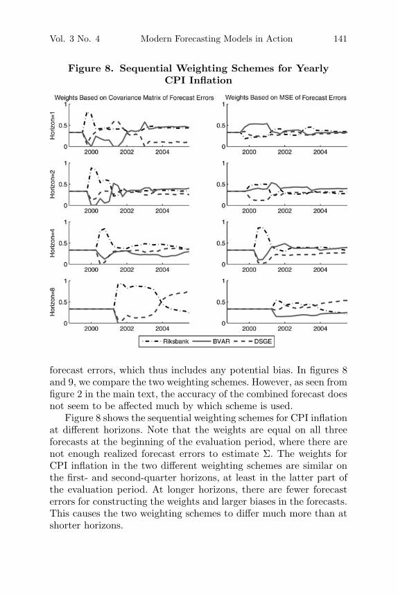
Figure 8. Sequential Weighting Schemes for YearlyCPI Inflation

forecast errors, which thus includes any potential bias. In figures 8and 9, we compare the two weighting schemes. However, as seen fromfigure 2 in the main text, the accuracy of the combined forecast doesnot seem to be affected much by which scheme is used.

Figure 8 shows the sequential weighting schemes for CPI inflationat different horizons. Note that the weights are equal on all threeforecasts at the beginning of the evaluation period, where there arenot enough realized forecast errors to estimate Σ. The weights forCPI inflation in the two different weighting schemes are similar onthe first- and second-quarter horizons, at least in the latter part ofthe evaluation period. At longer horizons, there are fewer forecasterrors for constructing the weights and larger biases in the forecasts.This causes the two weighting schemes to differ much more than atshorter horizons.


Figure 9. Sequential Weighting Schemes for theInterest Rate

For the interest rate, the sequential forecast weights are oncemore stable at the two shortest horizons compared with the longerones; see figure 9. From figure 9, it can also be seen that the supe-riority of the implicit forward rate at the first- and second-quarterhorizons is immediately picked up by both weighting schemes.

References

Adolfson, M., S. Laseen, J. Linde, and M. Villani. 2005. “AreConstant Interest Rate Forecasts Modest Policy Interventions?Evidence from a Dynamic Open-Economy Model.” InternationalFinance 8 (3): 509–44.


———. Forthcoming. “Evaluating an Estimated New KeynesianSmall Open Economy Model.” Journal of Economic Dynamicsand Control.

Altig, D. E., C. T. Carlstrom, and K. J. Lansing. 1995. “ComputableGeneral Equilibrium Models and Monetary Policy Advice.” Jour-nal of Money, Credit and Banking 27 (4): 1472–93.

Altig, D., L. Christiano, M. Eichenbaum, and J. Linde. 2003.“TheRole of Monetary Policy in the Propagation of TechnologyShocks.” Manuscript, Northwestern University.

Canova, F., and G. de Nicolo. 2002. “Monetary Disturbances Mat-ter for Business Fluctuations in the G-7.” Journal of MonetaryEconomics 49 (6): 1131–59.

Christiano, L. J., M. Eichenbaum, and C. L. Evans. 2005. “Nomi-nal Rigidities and the Dynamic Effects of a Shock to MonetaryPolicy.” Journal of Political Economy 113 (1): 1–45.

Del Negro, M., and F. Schorfheide. 2004. “Priors from General Equi-librium Models for VARs.” International Economic Review 45(2): 643–73.

Doan, T. A. 1992. RATS User’s Manual. Version 4. Evanston, IL:Estima.

Draper, D. 1995. “Assessment and Propagation of Model Uncer-tainty.” Journal of the Royal Statistical Society 57: 45–97.

Edge, R., M. Kiley, and J.-P. Laforte. 2006. “A Comparison ofForecast Performance Between Federal Reserve Staff Forecasts,Simple Reduced-Form Models, and a DSGE Model.” Manuscript,Board of Governors of the Federal Reserve System.

Faust, J. 2005. “Is Applied Monetary Policy Analysis Hard?”Manuscript, Board of Governors of the Federal Reserve System.

Jacobson T., P. Jansson, A. Vredin, and A. Warne. 2001. “Mone-tary Policy Analysis and Inflation Targeting in a Small OpenEconomy: A VAR Approach.” Journal of Applied Econometrics16 (4): 487–520.

King, R. G., C. I. Plosser, J. H. Stock, and M. W. Watson. 1991.“Stochastic Trends and Economic Fluctuations.” American Eco-nomic Review 81 (4): 819–40.

Litterman, R. B. 1986. “Forecasting with Bayesian VectorAutoregressions—Five Years of Experience.” Journal of Businessand Economic Statistics 4 (1): 25–38.


Sims, C. A. 2002. “The Role of Models and Probabilities in the Mon-etary Policy Process.” Brookings Papers on Economic Activity 2:1–62.

Smets, F., and R. Wouters. 2002. “Openness, Imperfect ExchangeRate Pass-Through and Monetary Policy.” Journal of MonetaryEconomics 49 (5): 947–81.

———. 2004. “Forecasting with a Bayesian DSGE Model: An Appli-cation to the Euro Area.” Journal of Common Market Studies42 (4): 841–67.

Svensson, L. E. O. 1995. “Estimating Forward Interest Rates withthe Extended Nelson and Siegel Method.” Sveriges RiksbankQuarterly Review 3: 13–26.

———. 2005. “Monetary Policy with Judgment: Forecast Target-ing.” International Journal of Central Banking 1 (1): 1–54.

Uhlig, H. 2005. “What Are the Effects of Monetary Policy on Out-put? Results from an Agnostic Identification Procedure.” Journalof Monetary Economics 52 (2): 381–419.

Villani, M. 2005. “Inference in Vector Autoregressive Models withan Informative Prior on the Steady State.” Sveriges RiksbankWorking Paper No. 181.

Waggoner, D. F., and Zha, T. 1999. “Conditional Forecasts inDynamic Multivariate Models.” Review of Economics and Sta-tistics 81 (4): 639–51.

———. 2003a. “A Gibbs Sampler for Structural Vector Autore-gressions.” Journal of Economic Dynamics and Control 28 (2):349–66.

———. 2003b. “Likelihood-Preserving Normalization in MultipleEquation Models.” Journal of Econometrics 114 (2): 329–47.

Winkler, R. L. 1981. “Combining Probability Distributions fromDependent Sources.” Management Science 27 (4): 479–88.

modern forecasting models in action: improving ... · pdf filemodern forecasting models in...

Documents