NOT FOR QUOTATION WITHOUT P E R M I S S I O N O F T H E AUTHOR

MODELS O F COMPLETE E X P E N D I T U R E SYSTEMS FOR I N D I A

R . R a d h a k r i s h n a K.N. M u r t y

M a y 1 9 8 0 W - 8 0 - 9 8

Working P a p e r s are i n t e r i m reports on w o r k of t h e I n t e r n a t i o n a l I n s t i t u t e f o r A p p l i e d S y s t e m s A n a l y s i s and have received o n l y l i m i t e d r e v i e w . V i e w s o r o p i n i o n s expressed h e r e i n do n o t necessa r i ly repre- s e n t those of t h e I n s t i t u t e o r of i t s N a t i o n a l M e m b e r O r g a n i z a t i o n s .

I N T E R N A T I O N A L I N S T I T U T E F O R A P P L I E D SYSTEMS A N A L Y S I S A - 2 3 6 1 L a x e n b u r g , A u s t r i a

PREFACE

Because food production is one of the most decentralized activities of mankind, and nations are the largest units in which agricultural problems appear in their full complexity, the activ- ities of the Food and Agriculture Program of IIASA are focused on the study of national food and agriculture systems. In order to study the world's food problems, a consistent set of national agricultural models is being developed. As a first step toward the realization of IIASA's objectives in modeling national food and agriculture systems, work has begun on the development of prototype models for countries representing various types of national agriculture systems.

Professor Kirit Parikh has developed a framework of the Indian agricultural policy model, as a prototype for Asian developing countries with limited food producing potential (RM-77-59).

The present report describes the modeling of a complete demand system for construction of an Indian Model. For the modeling of agricultural policy in a dveloping country, one needs a demand system that reflects the effect of income redis- tribution resulting from alternative government policies. This study, which describes an empirical estimation of such a complete demand system for India, is the second* in a set of studies which are to give empirical substance to the framework of the policy model for India and which will be published as part of a Research Report summarizing the results of the Indian Agri- cultural Model.

This study was initiated when Professor Radhakrishna visited IIASA, and was carried out together with Dr. Murty of the Sardar Pate1 Institute of Economic and Social Research, Ahmedabad, India. *The first one is a report describing the modeling of farm supply responses through empirical estimation.

iii

ACKNOWLEDGEMENTS

This study, carried out in collaboration with K.S. Parikh, has been tailored to a bigger study of the Agricultural Policy Model of India that is being carried out at IIASA. The model of the present study was formulated during the winter of 1978 while R. Radhakrishna was on a visit to IIASA. The stimulating discussions that he had with the research staff of IIASA, particularly with M.A. Keyzer, N.S.S. Narayana and K.S. Parikh had considerable impact on the final formulation of the model.

We are grateful to F. Rabax for initiating the study and extending support from IIASA, and to K.K. Subramanian for ex- tending his help from the Sardar Pate1 Institute of Economic and Social Research, Ahmedabad, India. Our thanks are also due to V.B. Tulasidhar and D.H. PariRh.

CONTENTS

1. INTRODUCTION Purpose Studies on Consumption Patterns of India Choice of the Model Commodity Classification

2. MODEL AND ESTIMATION Subgroup Model Estimation of LES

3. LINEAR EXPENDITURE SYSTEM Introduction Nine Commodity LES LES for 1 1 Commodity Groups Hierarchic Model Conclusions

NOTES REFERENCES APPENDIX

MODELS OF COMPLETE EXPENDITURE SYSTEMS FOR INDIA

R. Radhakrishna, K.N. rlurty

CHAPTER I INTRODUCTION

Purpose

The purpose of this study is' to estimate a suitable demand

model for the Agricultural Policy Model of India which is being

developed at the International Institute for Applied Systems

Analysis (Parikh, 1977). It is proposed to formulate the demand

model within the framework of a complete demand system and

structure it to handle the income redistributional effects in

a realistic manner. This could then meet the requirement of

endogenizing the price vector in the Agricultural Policy

Model. Though the demand model development was spurred by

the need of the IIASA agricultural policy model, we hope that

the model will also be useful for other analytical models

such as those designed to give demand projections under alter-

native distributions or policy models dealing with price

stabilization.

The Agricultural Policy Model is aimed at being a

descriptive model to evaluate the effectiveness of various

policies in the food and agricultural area. Since income

distribution plays a significant role in determining the

extent of malnutrition, and since income distribution is

affected by agricultural prices and terms of trade, bcth

prices and incomes are endogenous in the model. Moreover,

the objective of the IIASA project is also to study the

effects of international trade and aid policies. Thus the

economy is modeled as an open economy. The model is conceived

as a general equilibrium type model to be used in a year by

year simulation mode. A number of government policies are

also endogenous. For this model we need to estimate a complete

dernand system which can handle the effects of income re-

distribution resulting from alternative government policies.

We shall briefly review the studies that have been re-

ported on Indian Consumption Patterns. This will help us to

identify the considerations one has to take note of while

formulating the model.

STUDIES ON CONSUMPTION PATTERNS OF INDIA

Engel Curves

The availability of the ~ational Sample Survey (NSS) data

on consumer expenditure since 1950 has stimulated a large

number of studies on consumption patterns (Rudhra, 3969 and

Bhattacharya, 1975). However, most of the studies based on

this wealth of data in the past have been confined to the esti-

mation of Engel curves (Coondo, 1975 and Jain, 1975). The

expenditure elasticities obtained from them have become the

conceptual tools for demand projection making the following

assumptions: insensitivity of consumer expenditure to price

changes; invariance of income elasticities over time and price

structure. Projections made at the mean level further assume

away the changes in income distribution. These assumptions

appear unrealistic for a number of reasons. The influence

of prices both on household consumption and income elasticities

has been sharply brought into focus by the few studies carried

out recently on complete demand systems for India (Bhattacharya,

1967, Murty, 1977, Murty, 1978, Radhakrishna and Murty, 1973,

and Radhakrishna and Murty 1977). It would also be unrealistic

to ignore dependencies between shifts in income distribution and

demand projections, as there is a great deal of variation in the

scale of preferences among certain definable groups within the

economy. Income distributional effects may be ignored in case

the shifts in income distribution are marginal compared to total

growth. But in a developing country like India, it is well

established that frequent fluctuations in agricultural output

alter the income terms of trade.

Indifference Surfaces

In a few studies, quadratic utility functions have been

estimated from family budget data (Mahajan, 1972, Radhakrishna

and Murty, 1975, and Radhakrishna, 1977). The estimated

quadratic utility functions mostly violate the convexity

conditions. All other theoretical preconditions are satisfied

as they are built into the method of estimation. Further,

the quadratic utility function implies linear Engel curves

which are restrictive when the range of income variation is

wide. Further the methods of estimation are very data

demanding and the parameter estimates appear to be very

susceptible to measurement errors.

Linear Expenditure System (LES)

Among the Complete Demand Systems, the Linear Expenditure

Sys tem (LES) has received more attention; some have estimated

LES from the time series data (Bhattacharya, 1967), whilst

others from the time series of cross section data (Radhakrishna

and Murty, 1973). The LES gives satisfactory properties.

This is not surprising, since the additive utility func-

tions, to which LES conforms, are very rigid in specifica-

tion and ensure the fulfilment of almost all the theoretical

properties. They do not tell us whether the theoretical

properties do or do not hold in practice. We can only

explore whether they provide a satisfactory description

of consumer behavior a't a reasonable level of commodity

aggregation. The LES also gives rise to linear Engel curves.

The severity of this restriction can be moderated, to some

extent in time series models designed mainly for providing

predictions at the mean level without changes in income

distribution, either by introducing time trends into the

parameters (Stone, 1965) or by resorting to habit formation

hypothesis (Pollack and Wales, 1969). Even these moderations may

fail to forge a link between consumption patterns and income

distribution._

Piecewise LES (PLES)

Some attempts have been nade by Radhakrishna and Murty

at Sardar Pate1 Institute of Economic and Social Research

(SPIESR) to overcome some of the above limitations of LES

by the use of a piecewise LES. The NSS per capita expenditure

brackets of the rural and urban areas have been stratified

into three expenditure (income) classes viz., lower, middle

and higher and aseparate LES (with six and nine commodity groups)

has been fitted to each group. The results have clearly brought

out the suitability of the LES for local approximations and

show sizeable variations in the parameter estimates across the

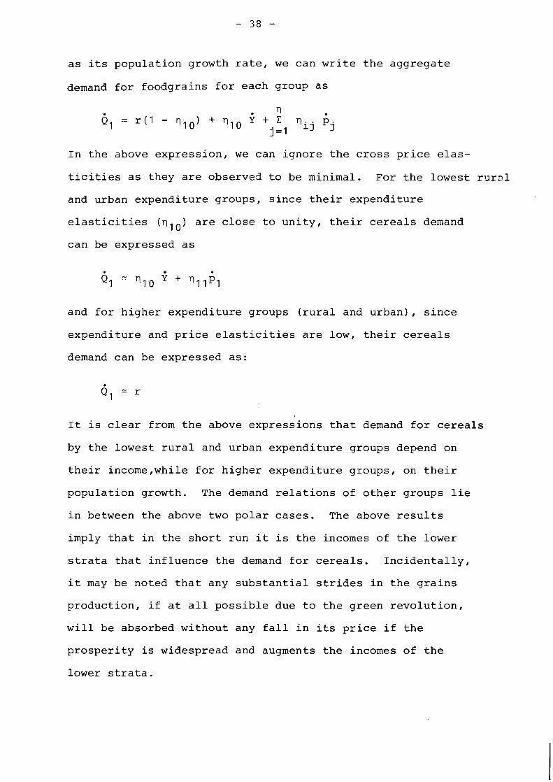
expenditure groups. For example, the foodgrains group takes

a major share of the total expenditure of the lower expend-

iture group (about 45 per cent in rural areas and 30 per cent

in urban areas) and its weightage reduces considerably as

the total expenditure level rises (to about 9 per cent in

rural higher expenditure group and 2 per cent in urban higher

expenditure group). The rural-urban variations are also

found to be sizeable: the marginal budgets of urban lower

and middle expenditure groups are more varied and diversified

than their counterparts in rural areas. Nevertheless, one

notices that in the case of a majority of items, variation

across income groups are more marked compared to rural-urban

differences for corresponding income groups.

Indirect Addilog System (IAS)

An attempt has also been made to examine whether the

Indirect Addilog System (IAS), a non-linear system, provides

a reasonable description of consumer behavior over the entire

income range (Radhakrishna and Murty, 1977). Both sample

and post sample predictions of the expenditures of various

income groups have shown that the IAS gives a poor fit for

lower income groups. From the above study it emerges that

the IAS is not flexible enough to provide a satisfactory

description of the consumer behavior over the entire range

of total expenditure (income). Thus, it brings out the

limitations of IAS in handling the distributional effects.

Piecewise IAS (PIAS)

Some attempts have also been made at the SPIESR to

estimate the IAS separately for each expenditure group. The

parameter estimates differ markedly across the expenditure

groups, thus reinforcing the need for distinguishing expenditure

groups. In a large number of cases, the IAS is found to

violate the convexity conditions. There is not much difference

between PLES and PIAS in terms of goodness of fit.

CHOICE OF THE MODEL

It would seem from the foregoing discussion that no

single complete demand system can adequately represent the

consumption patterns over a wide range of total expenditure

and one has to resort to grouping and estimate separate

models for each group. The choice is now between PLES and

PIAS. As pointed out in the preceding discussion, there is

not much to discriminate between the two models from the

point of view of goodness of fit. If one takes into con-

sideration the fulfilment of theoretical properties as a

desirable feature, the LES has a distinct edge over the IAS

since only LES fulfills all the theoretical properties and

the IAS violates convexity conditions. Further, consistency

in theoretical properties is an extremely desirable property

for the computation of exchange equilibrium in the Agricultural

Policy Models (Parikh, 1977). The above considerations have

led us to opt for the PLES.

COMMODITY CLASSIFICATION

Taking into consideration the availability of dzta and

the requirements of the Agricultural Policy Model, the

following commodity classification has been used as shown

in Table 1 below.

Table 1. Commodity list

Commodity Grcup Commodity I tems No Title Included

Rice Rice

Wheat Wheat

Other cereals Jowar, bajra, maize, barley, snall millets, ragi, Bengal gram and their products

Milk & milk Liquid milk, milk (condensed, products powered), ghee, butter, dahi,

ghol, lassi and other milk products

Edible oil Oil, oilseeds and products

Meat, egg & fish Meat, egg E fish

Sugar E gur Canned sugar, gur (unrefined sugar 1 and sugarcandy

Pulses

Fruits & vegetables

Other food

Clothing

T u ~ , gram, moong, masoor, urad, peas and thur products

Fruits and nuts, vegetables

Spices, beverages, refresh- ments and procured food; pickles, jams and jel.lies

Cotton (mill made, hand- woven and khadi) woollen, silk, rayon, etc., including bedding and upholstery

1 2 Fuel E light Coke, coal, firewood, electricity, gas, dung-cake, charcoal, kerosene, candle, matches and other lighting oil

1 3 Other non-food Pan, tobacco and its products, drugs and intoxi- cants, amusements and sports, education, medicine, toilets, rent,sundry goods, furniture, services, etc.

Formation of Income Groups

In earlier studies carried out at the SPIESR, the following

procedure has been adopted for the formation of income groups.

The LES has been estimated utilizing the data of all expenditure

classes. The signs of the residuals are found to have distinct

patterns across expenditure classes. The patterns are also

found to be stable over the periods. Taking into consideration

the signs of the residuals, three expenditure groups have been

formulated - the first four expenditure classes forming the

lower group, the next four forming the middle group and the last

four or five expenditure classes forming the higher expenditure

group. Since total expenditure is a monotonic function of income

we have also labeled total expenditure groups as income groups.

In the above grouping, the expenditure range of each expend-

iture group remains the same at current prices. However, with a

change in price level, the expenditure range of a group expressed

in terms of constant prices is likely to vary. In this study we

have taken into consideration price movements while formulating

the expenditure groups. Further, a finer disaggregation of

expenditure groups as compared to the previous study has been

adopted. In other words, the expenditure range in terms of

constant prices would remain the same and the expenditure groups

are more than three. In this scheme, given the current expenditure

of an individual at current price structure, we shall express

his current expenditure at base year prices by using appropriate

price deflators and locate his expenditure group.

We present below the grouping that has been adopted:

Taking into consideration the previous grouping and the require-

ments, we have formed five expenditure groups on the basis of

the 17th round expenditure classes at 1961,62 prices: RS. 0-8

forming the first group; 8-11, 11-13 the second group; 13-15,

15-18, 18-21 forming the third group; 21-24, 24-28, 28-34

forming the fourth group and 34-43, 43-55, 55-75, 75 and above

forming the fifth group. The class boundaries have then been

expressed at the price structures of other rounds by using

separate cost of living index for each class boundary and then

grouping has been made. The price deflators are taken from a

study by Radhakrishna and Atul Sarma (1975) carried out at SPIESR.

The study cited above gives cost of living indices for each

fractile class separately for the rural and urban areas. In

the end the following groupings of expenditure classes at constant

prices has emerged for the rural and urban areas (Figures la and

lb). It can be seen that expenditure classes contained in Group

I covers only the class Rs. 0-8 during the initial rounds but

covers classes Rs. 0-8, 8-11, 11-13, 13-15 and 15-18 during the

25th round. This is due to price rise.

Group I

I I

Group V

-

C

-

Group IV

-

- -

I

Group I11

-

Group I1

CHAPTER I1

MODEL AND ESTIMATION

We have utilized the LES which has been extensively

applied in analyzing the consumption patterns for a large

number of countries1- The LES is usually written in the

form

where qi represents the quantity consumed of ith commodity;

Pi is the price of ith commodity and y is total expenditure n

such that y = C vi . The b's and the c's are parameters i=l

of the system. The b's are the marginal budget shares and

c's are sometimes interpreted as committed quantities. This

interpretation is only suggestive and it is not always

possible to do so: particularly when c is negative. A i

negative c is not inconsistent with theory. The LES can be i

derived from maximization of the ordinal utility function.

n u(q) = C bi log (qi - ci) , C bi = 1

i= 1 i

subject to the budget constraint C piqi = p i

The fulfilment of the second order condition of

equilibrium requires that b.>O i.e. no inferior goods and 1

p>C c.p . Since it can be derived from a utility function, -i I j i

it meets the theoretical properties - adding up, homogeneity

and symmetry of the Slutsky substitution matrix. However,

the LES has a few limitations. Since the underlying utility

function is additive it becomes an unrealistic specification

when we deal with finer level of commodity aggregation. The

additivity, besides not allowing inferior goods, imposes too

strong a specification on price effects. Nevertheless, this

may not pose a problem for broad groups of consumption.

For commodity i the income elasticity T-- io ' own price

elasticity q and cross price elasticity with respect to ii th price qij are given by

- "io - biJwi

Subgroup Model

Though the NSS reports provide information on expenditure

for broad groups of consumption for a good many number of

rounds, they provide information for specific items, only for

a few rounds. Under these circumstances, the best strategy

would be tc estimate the LES in a hierarchical manner (Stone,1965,

Deaton,1974a). We may carry out the calculations first for the

broad groups and then for subgroups. The first stage model

can be estimated from data from a large number of rounds

while the subgroup models from the data of a few rounds. The

first stage model and the second stage model can be integrated

as follows.

We shall denote indices by capital letter subscripts and

assume that n individual goods are partitioned into G groups.

th Let us consider G group. Summing over all goods belonging

to Gth group and writing v for the group expenditure, we G

have

The above expression can be written in a form identical to

Eqn. 1 by defining group price indices pG , as

and the corresponding quantity indices qG , as

These may be substituted in Eqn. 3 to give the group equivalent

of Eqn. 1 as:

Turning to subgroups, the equations of the items belonging

to Gth group can be written as:

It can be seen that the parameters of the first stage model

(Eqn. 6) and subgroup models (Eqn. 7) together give the

estimates of model (Eqn. 1 . ) . It can be seen from the above

expressions that for consistent grouping, the weights of the

group price indices (Eon. 4 ) should be Ci which can be estimated

from subgroup models. In other words, we have to estimate

the sub models first, compute the group price indices.and

then estimate the first stage models. In practice, base

year budget proportions are used for compiling the group

price indices. Since individual prices are mostly collinear ,

these indices are likely to give d o s e approximation (see

Deaton, 1974a, pp. 159-161).

Estimation of LES

Let us introduce error terms in the LES and write it as

In the above equations R is singular because of the adding

up property which implies that i'R = 0 . Let us formulate

the likelihood function for Eqn. 8 by deleting one equation

for each t; without loss of generality we delete the last

equation . Denoting the truncated residuals as i t r

truncated b as 6 and truncated R as 6, the likelihood in logarithmic form can thus be written as

Since the first order conditions of the maximum likelihood

function give rise to nonlinear equations in parameters, the

maximum likelihood estimates can only be obtained by employing

iterative methods. Let us employ the linearization method

which yields the m.1. estimates (Solari, 1971, and Slater, 1972)"

th Linearizing the LES after deleting the n equation

- around an initial value bo and co we have

The above equations are linear in 65 and 6c . They

can be estimated by employing the maximum likelihood method

developed for seemingly unrelated regressions. The iteration

continues till 6b and 6c become negligible.

The above procedure does not yield an estimate of bn . It can, however, be evaluated from 6 by employing the adding

up property.

The estimation of hierarchic model poses some econometric

problems for the subgroup models. The total expenditure of

the first stage model (broad group model) can be taken as

predetermined and the model is concerned with its allocation;

the errors sum to zero and the co-variance between E and p i

is zero. However, in the case of subgroup model, the group

expenditure v cannot be taken as predetermined; the errors G

in each expenditure on the specific items get reflected in

the group expenditure and this does not ensure the absence

of co-variance between the errors in the expenditure on

specific items and the error in their group expenditure.

This introduces simultaneous equation bias in the estimation

of subgroup model and makes the estimates inconsistent.

Nevertheless, the bias is likely to be small (see Deaton,

1974a, pp. 165-168).

CHAPTER I11

LINEAR EXPENDITURE SYSTEM

Introduction

It is possible, using the NSS data on monthly per capita

expenditure, to distinguish nine commodity groups for which

data are available for a good many number of the NSS rounds.

It js also possible to distinuuish eleven commodity groups

for some rounds in the sample period. A few rounds of data

also permit us to estimate two submodels - one for cereals and the other for other food. The details of the commodity

classifications are given in Table 2.

The LES has been estimated by using the linearization

iterative procedure stated in Chapter I1 for all the ten

expenditure groups (Rural and Urban) defined in Chapter I.

Though we have estimated LES with 9 and 1 1 commodity classi-

fication, we have made use of the results of the 9 commodity

LES while drawing policy implications. The data are

abundant for 9 commodity groups. Further, additivity may

not be very restrictive at this level of commodity aggregation.

Nine Commodity LES

Fitting of the Model

LES has been estimated making two alternative specifi-

cations for the covariance of the disturbance terms. In

2 model I we have assumed that Q = a I and model I1 we have

assumed that non-diagonal terms of Q exist.

We have employed the linearization procedure while

estimating the mosels. It may be noted that no equation has

been deleted while estimating model I.

Table 2. Commodity classification

First Stage Models:

9 Sector LES

1. Cereals 2. Milk & milk products 3. Edible oil 4. Meat, egg & fish 5. Sugar & gur 6. Other food 7. Clothing 8. Fuel S light 9. Other nonfood

Other Food Subarou~

1. Pulses 2. Fruits & vegetables 3. Other food

1 1 Sector LES

Rice Wheat Other cereals Milk & milk products Edible oil Meat, egg & fish Sugar & gur Other food Clothing Fuel & light Other non-food

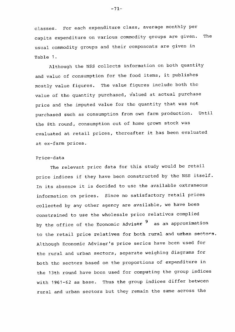
The data needed for estimating the models are taken from

4 the NSS reports for the rounds 2-25 - The group price indices

with prices for 1961-62 as unity are compiled from the

5 Economic Adviser's wholesale price relatives .

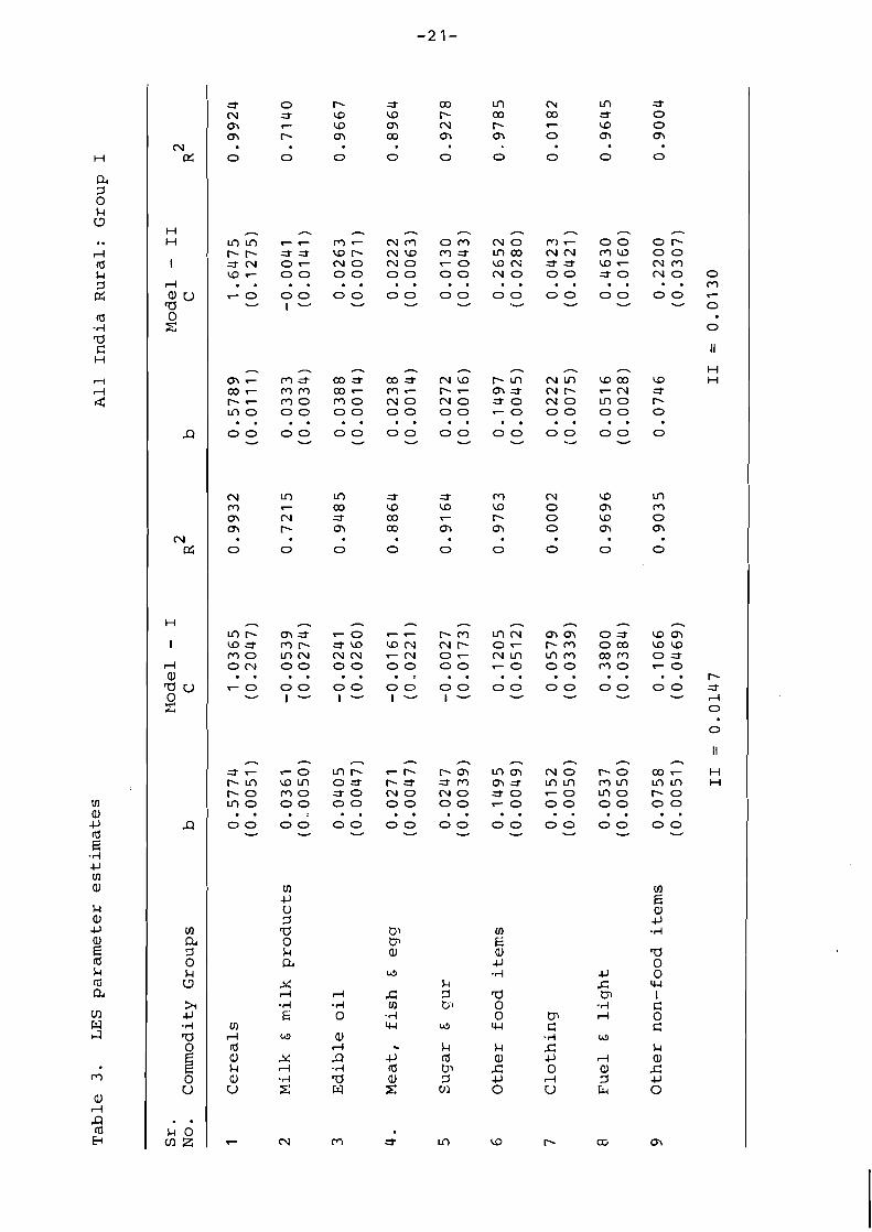
Parameter Estimates

The parameter estimates along with the standard errors

of the generalized least squares6 estimates of the linearized

LES at the last iteration which provide approximate confidence

contours (see Goldfeld and Quandt, 1972, p. 52, and Deaton,

1974b, pp. 45-46), are also given below the paramters in

Table 3.

In order to examine the goodness of fit, we have computed

for each commodity group, the value of the square of the

correlation coefficient between the observed and predicted

2 expenditures ( R ) for the sample period. The above goodness

of fit measure is also supplemented by Thiel's average infor-

mation inaccuracy ( I ) , T h e , 1975) given by A

Where w stands for the proportion of expenditure devoted to it

ith item in tth period. These goodness of fit measures are

also furnished in thefollowing Table along with the parameter

estimates of LES.

n n n n n n n n H m 7 m 3 a* a = N W ~ m ~ m wco w H 00.- m m a , ~ m - m a N P 7- a P Y m o m o N O N O a o N O m o P m a O C 00 00 00 70 00 00 0 . . . . . . . . . . . . . . . .

T a b l e 3 c o n t d . A l l I n d i a R u r a l : G r o u p I1

S r . Model - I Model - I1 N o Commodi ty G r o u p s b C R~ b C R~

1 C e r e a l s

2 M i l k & m i l k p r o d u c t s 0 . 0 7 7 5 ( 0 . 0 1 4 8 )

3 E d i b l e o i l

4 Meat, f i s h & e q g 0 . 0 3 6 9 ( 0 . 0 1 0 8 )

5 S u g a r & q u r

6 O t h e r f o o d i t e m s 0 . 1 3 8 8 ( 0 . 0 1 2 8 )

7 C l o t h i n g

8 F u e l & l i g h t

9 O t h e r n o n - f o o d i t e m s 0 . 1 1 0 6 0 . 0 8 9 2 0 . 9 3 0 2 0 . 0 8 3 2 0 . 2 6 5 3 0 . 9 2 8 9 ( 0 . 0 1 1 9 ) ( 0 . 1 2 4 3 ) ( 0 . 0 9 2 1 )

n

N 7 03 l- o m 0 0 . . 0 0

I'

h

7 w l- l- a o 7 0 . . 0 0 w

l- a 7

m

0

n

03 N l-w l- 0 N N . . 0 0

I W

n

w a w a m 7 7 0 . . 0 0 w

2 a, c,

0 tn -4 0 a, 5 a

c, a -4

0 c,

k 0

Jl w ~l 3 a 0 I m 0 0 -4 -4

C 0 0 r l . u b3 'G

0 C -4 a

C C k k Jl k c, rd a, c, rl Q) a 0 Jl 0 a, Jl

s 7 c, rl 7 c, rn 0 u Frc 0