models meet data: challenges and opportunities in
TRANSCRIPT
R E S E A R CH R E V I EW
Models meet data: Challenges and opportunities inimplementing land management in Earth system models
Julia Pongratz1 | Han Dolman2 | Axel Don3 | Karl-Heinz Erb4 |
Richard Fuchs5 | Martin Herold6 | Chris Jones7 | Tobias Kuemmerle8,9 |
Sebastiaan Luyssaert2 | Patrick Meyfroidt10,11 | Kim Naudts1
1Max Planck Institute for Meteorology,
Hamburg, Germany
2Department of Earth Sciences, VU
University Amsterdam, Amsterdam, The
Netherlands
3Th€unen-Institute of Climate-Smart
Agriculture, Braunschweig, Germany
4Institute of Social Ecology Vienna (SEC),
Alpen-Adria Universitaet Klagenfurt Wien,
Graz, Vienna, Austria
5Geography Group, Department of Earth
Sciences, Vrije Universiteit Amsterdam,
Amsterdam, The Netherlands
6Laboratory of Geoinformation Science and
Remote Sensing, Wageningen University
and Research, Wageningen, The
Netherlands
7Met Office Hadley Centre, Exeter, UK
8Geography Department, Humboldt-
Universit€at zu Berlin, Berlin, Germany
9Integrative Research Institute on
Transformations of Human-Environment
Systems (IRI THESys), Humboldt-Universit€at
zu Berlin, Berlin, Germany
10Georges Lemaıtre Center for Earth and
Climate Research, Earth and Life Institute,
Universit�e Catholique de Louvain & F.R.S.-
FNRS, Louvain-la-Neuve, Belgium
11F.R.S.-FNRS, Brussels, Belgium
Correspondence
Julia Pongratz, Max Planck Institute for
Meteorology, Hamburg, Germany.
Email: [email protected]
Funding information
International Space Science Institute (Bern);
German Research Foundation’s Emmy
Noether Program, Grant/Award Number: PO
1751/1-1; Fonds de la Recherche
Scientifique (F.R.S.-FNRS/Belgium); Joint UK
BEIS/Defra Met Office Hadley Centre
Abstract
As the applications of Earth system models (ESMs) move from general climate pro-
jections toward questions of mitigation and adaptation, the inclusion of land man-
agement practices in these models becomes crucial. We carried out a survey among
modeling groups to show an evolution from models able only to deal with land-
cover change to more sophisticated approaches that allow also for the partial inte-
gration of land management changes. For the longer term a comprehensive land
management representation can be anticipated for all major models. To guide the
prioritization of implementation, we evaluate ten land management practices—for-
estry harvest, tree species selection, grazing and mowing harvest, crop harvest, crop
species selection, irrigation, wetland drainage, fertilization, tillage, and fire—for (1)
their importance on the Earth system, (2) the possibility of implementing them in
state-of-the-art ESMs, and (3) availability of required input data. Matching these
criteria, we identify “low-hanging fruits” for the inclusion in ESMs, such as basic
implementations of crop and forestry harvest and fertilization. We also identify
research requirements for specific communities to address the remaining land man-
agement practices. Data availability severely hampers modeling the most extensive
land management practice, grazing and mowing harvest, and is a limiting factor for a
comprehensive implementation of most other practices. Inadequate process under-
standing hampers even a basic assessment of crop species selection and tillage
effects. The need for multiple advanced model structures will be the challenge for a
comprehensive implementation of most practices but considerable synergy can be
gained using the same structures for different practices. A continuous and closer
collaboration of the modeling, Earth observation, and land system science communi-
ties is thus required to achieve the inclusion of land management in ESMs.
K E YWORD S
climate, croplands, Earth observations, Earth system models, forestry, grazing, land
management, land use
- - - - - - - - - - - - - - - - - - - - - - - - - - - - - - - - - - - - - - - - - - - - - - - - - - - - - - - - - - - - - - - - - - - - - - - - - - - - - - - - - - - - - - - - - - - - - - - - - - - - - - - - - - - - - - - - - - - - - - - - - - - - - - - - - - - - - - - - - - - - - - - - - - - - - - - - - - - - - - - - - - - - - -This is an open access article under the terms of the Creative Commons Attribution License, which permits use, distribution and reproduction in any medium,
provided the original work is properly cited.
© 2018 The Authors. Global Change Biology Published by John Wiley & Sons Ltd
Received: 31 August 2017 | Accepted: 18 October 2017
DOI: 10.1111/gcb.13988
1470 | wileyonlinelibrary.com/journal/gcb Glob Change Biol. 2018;24:1470–1487.

Climate Programme, Grant/Award Number:
GA01101; EU H2020 project CRESCENDO,
Grant/Award Number: 641816; FP7 LUC4C,
Grant/Award Number: 603542; NESSC
Netherlands Earth System Sensitivity Centre;
European Space Agency Land Cover CCI
Project; ESA GOFC-GOLD; ERC-Stg 263522
LUISE
1 | INTRODUCTION
Three quarters of the Earth’s ice-free land surface are in some form
managed by humans (Luyssaert et al., 2014). While this provides
essential food, fiber, energy, and living space for about 7 billion peo-
ple (Haberl et al., 2007), the extent and magnitude of land-use
change impacts key Earth system processes, including the climate, in
major ways. Global climate change has been accelerated by green-
house-gas emissions from land-use changes, with about one-third of
all anthropogenic CO2 emissions over the industrial era attributable
to deforestation (Houghton, 2003). In addition, changes in albedo,
energy fluxes, and water fluxes induce changes in surface climate as
important locally as those induced by the increased global green-
house-gas concentration (de Noblet-Ducoudr�e et al., 2012), which
can feed back on atmospheric dynamics on regional scale (Winckler,
Reick, & Pongratz, 2017). Understanding how different types of land-
use change affect climate-relevant parameters is therefore important.
This requires bridging different Earth system science disciplines,
particularly the climate change and land system science communities,
and establishing a common terminology. Here, we use the term
land-use change as an umbrella to entail both conversion from one
broad land-use class to another (e.g., from forestry to cropping) and
changes in land management within one land-use class (e.g., intensi-
fication of cropping). Importantly, this moves beyond simplified defi-
nitions that defined land-use change by its impact on land cover to
define land-use change more comprehensively and mechanistically
(see Figure 1). Both land-use conversions and land management
impact the climate through biogeochemical and biogeophysical path-
ways.
Earth system models (ESMs) have become key tools to assess
how land-use change has affected the climate in the historical past
and how it may affect the climate for future scenarios. The Coupled
Model Intercomparison Project 5 (CMIP5), which provided the simu-
lations underlying the Intergovernmental Panel on Climate Change
(IPCC) 5th Assessment Report, was the first CMIP that included spa-
tially explicit maps of land-use change as a forcing (Hurtt et al.,
2011) in addition to industrial greenhouse-gas fluxes. At this stage,
models were limited in the types of land-use change represented:
Most models represented anthropogenic conversions in land use,
typically those that also result in land-cover conversions such as the
clearing of natural vegetation for cropland expansion (Boysen et al.,
2014; Brovkin et al., 2013). These are relevant for about 18-29% of
the ice-free land surface, while land management, inducing both
land-cover conversions and modifications, affects about 71%–76% of
the land (Luyssaert et al., 2014). Nevertheless, the effects of land
management were practically absent in CMIP5. Only some ESMs
accounted for land management practices like wood harvest (e.g.,
Shevliakova et al., 2013; Wilkenskjeld, Kloster, Pongratz, Raddatz, &
Reick, 2014).
However, observational evidence points toward land manage-
ment inducing important effects on surface climate (Luyssaert et al.,
2014). Individual modeling studies confirm that land management
practices such as irrigation (Boucher, Myhre, & Myhre, 2004), crop
harvest (e.g., Pugh et al., 2015), no-till (Davin, Seneviratne, Ciais,
Olioso, & Wang, 2014), grazing (Eastman, Coughenour, & Pielke,
2001), or forestry practices (Naudts et al., 2016) can notably alter
biogeophysical properties and biogeochemical cycles in large regions
of the world. A recent comparison study of several land surface
models (LSMs) for certain land management practices revealed that
emissions from land use may be consistently underestimated by ear-
lier assessments accounting only for anthropogenic land-cover con-
versions (Arneth et al., 2017), challenging our understanding of
terrestrial carbon sources and sinks.
Beyond this evidence of important effects on the Earth system
land management becomes increasingly important in the context of
climate policy. Land use in general is a tool to mitigate global climate
change (UNFCCC, 2005). Given that intensification will play a deci-
sive role in fulfilling the surging future demand for land-based food,
feed, and fiber (Erb, Lauk, et al., 2016; Foley et al., 2011), land man-
agement choices provide a key lever for future mitigation and adap-
tation (Erb, Haberl, & Plutzar, 2012; Smith et al., 2013). A key issue
is to assess the trade-offs between intensification through changes
in land management and further expansion into natural ecosystems
(Kuemmerle et al., 2013; Lambin et al., 2013). Policy decisions
around land-based mitigation activities, such as biofuel, need to be
informed by both biogeochemical and biophysical implications of
such actions.
For these reasons moving beyond conversions in land use that
induce land-cover conversions to also represent land management
has become a key priority for Earth system modeling. This is also
reflected in additional data layers provided for CMIP6 and proposed
simulations that isolate management effects and compare them
across models (Lawrence et al., 2016). Assessments of regional land
management strategies with promise to help mitigate and/or adapt
to climate change are envisaged within the Land Use Model Inter-
comparison Project (LUMIP) (Lawrence et al., 2016).
A model extension toward land management further provides a
direct link between ESMs and integrated assessment modeling (IAM)
by sharing common input and output variables, such as amount of
irrigation and fertilization or forest and agricultural yields. Land
PONGRATZ ET AL. | 1471

management thus provides a way to test and improve the consis-
tency between these two types of models. IAMs and ESMs have so
far been linked only loosely due to both methodological and data
challenges (Prestele et al., 2017) and the fact that feedbacks
between environmental and human systems in many cases are small
(Van Vuuren et al., 2012). However, land management and land-use
conversions are a prime example for where these feedbacks may be
non-negligible because of the tight coupling of the land surface with
the atmosphere and of the land surface state with human decision
making (Van Vuuren et al., 2012). First attempts at synchronously
coupling IAMs and ESMs therefore exist (e.g., Collins et al., 2015)
and show, for example, a decrease in projected managed area when
beneficial effects on plant productivity such as increasing atmo-
spheric CO2 levels are accounted for (Thornton et al., 2017).
Given that human and computational resources are limited, ESM
groups need to prioritize which management practices should be
implemented preferentially. This process can be guided by the fol-
lowing criteria:
(1). Model or observation-based evidence shows that the effects
of a land management practice on the Earth system are
substantial.
(2). The spatial extent that a land management practice covers is
large.
(3). Processes relating a land management practice to its biophysical
and biogeochemical effects need to be sufficiently understood
to be implementable in a process-based model.
(4). The current concepts and structures underlying ESMs are suffi-
cient or can easily be adapted to capture the land management
practice.
(5). The data required to drive ESMs extended by a land manage-
ment practice need to be available. Also, specific evaluation
datasets would ideally be available.
The first two of these criteria are related to the prospective
impact of the land management practice on the Earth system, the
third and fourth to the implementation in ESMs, with the last relating
to data availability for any realistic simulation. Studies have assessed
the spatial extent of various practices and gathered evidence of land
management effects (see Luyssaert et al., 2014; and Erb, Luyssaert,
et al., 2016; for reviews). A recent study has reviewed the current
state of knowledge of major land management practices with respect
to the level of process understanding of Earth system impacts and
data availability of the underlying drivers (Erb, Luyssaert, et al., 2016).
Land Cover (LC):Physical properties of a land surface
Land Use (LU):Purpose for and activities by which humans use land
User-defined categories
Land
use
cha
nge
Broad LU classes
Specific LU classes
Land use conversion (categorical properties)
Land management change(continuous properties)
No simple 1:1 relationships
Grassland
Forest
Bare soil
Coniferous F. Mixed F. Broadleaved F.
Broad LC classes
Specific LC classes
Forestry
Cropping
Grazing
Wheat Maize Fodder
Land cover conversion (categorical properties)
Land cover modification(continuous properties)
Land
cov
er c
hang
e
F IGURE 1 Clarifying land-use terminology. Clarifying basic terminology in terms of land-use change and land-cover change is essentialgiven that these terms are not always used consistently in the climate change and land system science communities. Land cover is defined asthe sum of all land surface properties at a given location (e.g., biophysical, morphological, topographical) and typically described by vegetationand soil characteristics at that location. Land cover is often categorized in broad land-cover classes (e.g., forest, grassland, bare ground), whichcan be subdivided into more detailed classes (e.g., deciduous forest, coniferous forest, mixed forest). Land-cover maps can provide one classlabel or a continuous class proportion (e.g., % tree cover) for each gridcell. Land use relates to the purposes or functions that humans assign toa given location and how humans interact with the land. Land use is also typically categorized in broad classes (e.g., forestry, grazing, cropping).Land management refers to the land-use practices that take place within these broader land-use classes (e.g., sowing, fertilizing, weeding,harvesting, thinning, clear-cutting). Land-use change over time then refers to either (a) conversions among broad land-use classes (e.g.,agricultural expansion) or (b) changes in land management within these classes (e.g., agricultural intensification). Importantly, both types ofland-use changes can result in either (i) land-cover conversion from one class to another (e.g., forest loss), or (ii) in more subtle changes inecosystem properties (e.g., forest degradation), denoted as land-cover modifications. Some previous studies and reviews (e.g., Erb, Luyssaert,et al., 2016; Luyssaert et al., 2014) used simplified terminology, assuming that land-use conversion always lead to land-cover conversion, andland management changes to land-cover modifications. While this is often the case, it is important to note that the terms land cover and landuse are not congruent, as land management can lead to land-cover conversions (e.g., wood harvesting resulting in the full clear-cutting offorest), and land-use conversion can happen without drastic changes in land cover (e.g., putting livestock on natural grasslands)
1472 | PONGRATZ ET AL.

We lack, however, an assessment of ways to implement land
management practices in current ESM structures. Further, data avail-
ability needs to be matched with modeling needs to guide prioritiza-
tion in the observational community for collection of additional
datasets. This study will address these gaps. Here, we focus on
implementing the ten land management practices that were selected
by Erb, Luyssaert, et al. (2016) based on their global prevalence
across a diversity of biomes and the strength of their biogeophysical
and biogeochemical effects on the Earth system, as described in the
literature. These 10 land management practices are: (1) forestry har-
vest; (2) tree species selection; (3) grazing and mowing harvest; (4)
crop harvest and crop residue management; (5) crop species selec-
tion; (6) fertilization of cropland and grazing land; (7) tillage; (8) crop
irrigation (including paddy rice irrigation); (9) artificial drainage of
wetlands for agricultural purposes; and (10) fire as a management
tool. We will discuss the status of implementation of land manage-
ment in ESMs, possible implementation approaches for these ten
practices, and data availability for model input and evaluation. This
study will thus identify challenges and opportunities for the assess-
ment of land management effects in Earth system research and allow
for a comprehensive prioritization of various land management prac-
tices.
2 | STATUS OF LAND MANAGEMENT INEARTH SYSTEM MODELS
2.1 | Current state of implementation
We conducted a survey among modeling groups participating in
international studies including land-use change (SOM text S1).
Hence, by design, all 17 models who participated currently represent
land-use change in some form. Prior to the inclusion of land-use
change, ESMs typically already included a submodel for natural vege-
tation processes, to account for processes such as changes in bio-
geographical distribution of natural vegetation or wildfires (Figure 2).
Yet, this does not imply that the link between natural processes and
land-use change is well developed. For instance, models disagree on
if and how fire should be represented on managed areas (e.g., Rabin
et al., 2017) and few models feature an explicit interaction of natural
and anthropogenic land-cover modifications, such as the preferential
allocation of pasture on natural grasslands (e.g., Schneck, Reick, Pon-
gratz, & Gayler, 2015).
As climate models moved toward ESMs, the carbon cycle was
included to prognostically calculate the atmospheric CO2 concentra-
tion and capture this dominant driver of anthropogenic climate
change (Flato et al., 2013). The carbon cycle is thus represented
more frequently than nitrogen or phosphorus cycles. In fact, simu-
lated land surface emissions of non-CO2 greenhouse gases are
implemented in only around one-third of all models considered in
our survey (Figure 2). Forest and crop harvest and the correspond-
ing product pools as well as subgrid scale transitions, which all
directly alter vegetation and soil carbon stocks, are the most com-
mon processes related to land management that are considered in
current ESMs (Figure 2). It is worth emphasizing that the develop-
ment of increasingly complex biophysical models on the one hand
and biogeochemistry models on the other hand not necessarily
implies that the two are integrated. For example, only three of nine
participating models also include tree age classes, but a representa-
tion of forest structure is needed to capture the biophysical effects
of wood harvest in addition to the biogeochemical effect (e.g., Otto
et al., 2014). Similarly, models might represent the release of carbon
from fires while the feedback on the biophysical part through
(b)
(a)
F IGURE 2 Percentage of (a) integratedassessment models and (b) Earth systemmodels representing various processesrelated to the conversion in land use orland management. The different colorsindicate different generations of models:present use (Generation 1), currentdevelopment cycle (Generation 2), andplans beyond the Coupled ModelIntercomparison Project 6 (CMIP6)(Generation 3)
PONGRATZ ET AL. | 1473

albedo may not exist in the model (e.g., Lasslop, Thonicke, & Klos-
ter, 2014).
Despite the small number of IAMs participating in our survey,
some clear differences and common features emerge in the treat-
ment of land management between ESMs and IAMs: Forest and crop
harvest are important practices also in IAMs (Figure 2), although the
focus is on their socioeconomic importance, rather than for carbon
cycling as in the ESMs. This different focus of IAMs and ESMs is
reflected in the subordinate role of processes related to natural
vegetation and vegetation dynamics in IA modeling (Figure 2).
2.2 | Planned implementations
Ongoing activities aim at moving ESMs toward an extension of bio-
geochemical cycles and greenhouse-gas fluxes beyond carbon, but
also to implement more detail on agricultural management (Figure 2).
Some land management practices, such as fertilization and irrigation,
are well captured by crop models (e.g., Brisson et al., 2003), and
currently move to the focus of the ESM community due to the
emerging empirical evidence of their substantial biogeophysical (in
particular for irrigation) and biogeochemical effects (in particular for
fertilization, grazing, and residue management) (see Erb, Luyssaert,
et al., 2016, for a detailed review).
With these plans, there is a clear trend toward a more complete
representation of land-use change, including land management
effects, in ESMs from the current state to the perspective beyond
CMIP6 (Figure 3). A tendency appears for models to compensate for
their “weaknesses” first by improving on the aspect, either forestry
or agricultural management, which was more coarsely represented
before (Figure 3). It needs to be noted that development paths
across models have similarities because dependencies of certain pro-
cesses on others are the same for all models, for example, the
requirement of a nitrogen cycle for fertilization (see also Figure 4).
The long-term consequence of the planned developments is a con-
vergence of models toward a detailed representation of land man-
agement. However, on the timescales covered here (several years
beyond CMIP6) the diversity and amount of processes that can be
represented in the face of limited resources will keep models
dissimilar (the models do not converge yet at the highest complexity
in Figure 3). Representation of the same process also differs
between models, meaning that even models with the same degree
of complexity can exhibit marked differences in their simulated
behavior and sensitivity. The development path taken by each model
to add a more comprehensive representation of land management
thus differs based on current capabilities and different prioritization.
While it must be expected that in the medium term, as models
start to implement different land management practices, model
spread will increase, the common trend toward high complexity (Fig-
ure 3) suggests that models eventually converge on a more homoge-
neous accounting for land-use conversions and land management
processes alike. Currently, studies applying several LSMs for their
estimates of land-use change impacts on surface climate and biogeo-
chemical fluxes typically rely on multimodel mean and spread for a
best estimate (e.g., Le Qu�er�e et al., 2015) despite the fact that the
amount and types of land-use and land management practices differ
across models. For example, in LUCID-CMIP5 (“Land-Use and
F IGURE 3 Representation of land management in ten Earth system and three integrated assessment models (all models from our survey(text S1) that provided information for all three development cycles). Solid lines connect present use and current development cycle, dashedlines current development cycle with plans beyond CMIP6. The completeness score reflects how many of forest management and agriculturalmanagement processes and variables are considered in the models. For forest management the maximum score of four reflects that (1) woodharvest, (2) forest age classes, (3) the fate of harvest, and (4) the fate of residues are considered. For agricultural management the maximumscore of nine would include (1) cropland presentation, (2) crop harvest, (3) fate of harvest, (4) crop residues, (5) fertilizer use, (6) use ofirrigation, (7) inclusion of other greenhouse gases, (8) grazing, and (9) pasture management. A score of zero means that none of them areincluded
1474 | PONGRATZ ET AL.
Climate, IDentification of robust impacts” in CMIP5) only three of six
models accounted for pasture as a specific plant functional type,
three models accounted for subgrid scale transitions, and one model
accounted for wood harvest (Brovkin et al., 2013). The inclusion of
more land management practices will in the future allow to form lar-
ger ensembles of models that account for the same processes, as
currently part of the spread across models must still be attributed to
different land-use change processes included (Houghton et al.,
2012). Moving toward a greater comprehensiveness will also facili-
tate evaluation of models against observations. For instance, Nya-
wira, Nabel, Don, Brovkin, and Pongratz (2016) found that the
observed sign of soil carbon changes for forest-cropland transitions
could be simulated by a LSM only after the inclusion of crop har-
vesting.
3 | IMPLEMENTATION OF TEN LANDMANAGEMENT PRACTICES IN EARTHSYSTEM MODELS
3.1 | Basic and comprehensive implementationapproaches
We outline possible approaches of implementation of the ten man-
agement practices to assess the required implementation efforts and
associated need for data. The starting point for the suggested
approaches is a typical land surface component of an ESM that is
capable of representing land-cover conversions (Boysen et al., 2014;
Brovkin et al., 2013). We acknowledge that individual models may
differ substantially in their process description, but common histories
and fundamental approaches (Fisher, Huntzinger, Schwalm, & Sitch,
2014) allow for capturing common features across a wide range of
models. While many effects of certain land management practices
require no structures beyond those contained in typical LSMs, but
only additional detail (e.g., the introduction of product carbon pools
for harvested material in parallel to existing soil and vegetation car-
bon pools), other effects require processes to be implemented that
were previously ignored or implicitly parameterized (such as prog-
nostic groundwater storage).
Since the representation of a land management practice in a
model can vary substantially in its level of comprehensiveness, we
describe possible approaches on two levels: A “basic” implementa-
tion aims at capturing some of the most obvious effects of a prac-
tice (e.g., biomass removal for forest harvest), i.e., fulfills the
minimum requirement for a model to account for this practice. A
more “comprehensive” implementation accounts for details of how
the practice is realized (e.g., harvesting of differently aged forest and
influencing canopy structure). The aim of the latter is a comprehen-
sive depiction of effects on the Earth system, although some of
these effects are marginal (Erb, Luyssaert, et al., 2016). As the key
purpose of assessing basic and comprehensive implementations is to
span the range of methods for the prioritization, the exact distinc-
tion is not crucial. Table S2 summarizes the need of additional input
data.
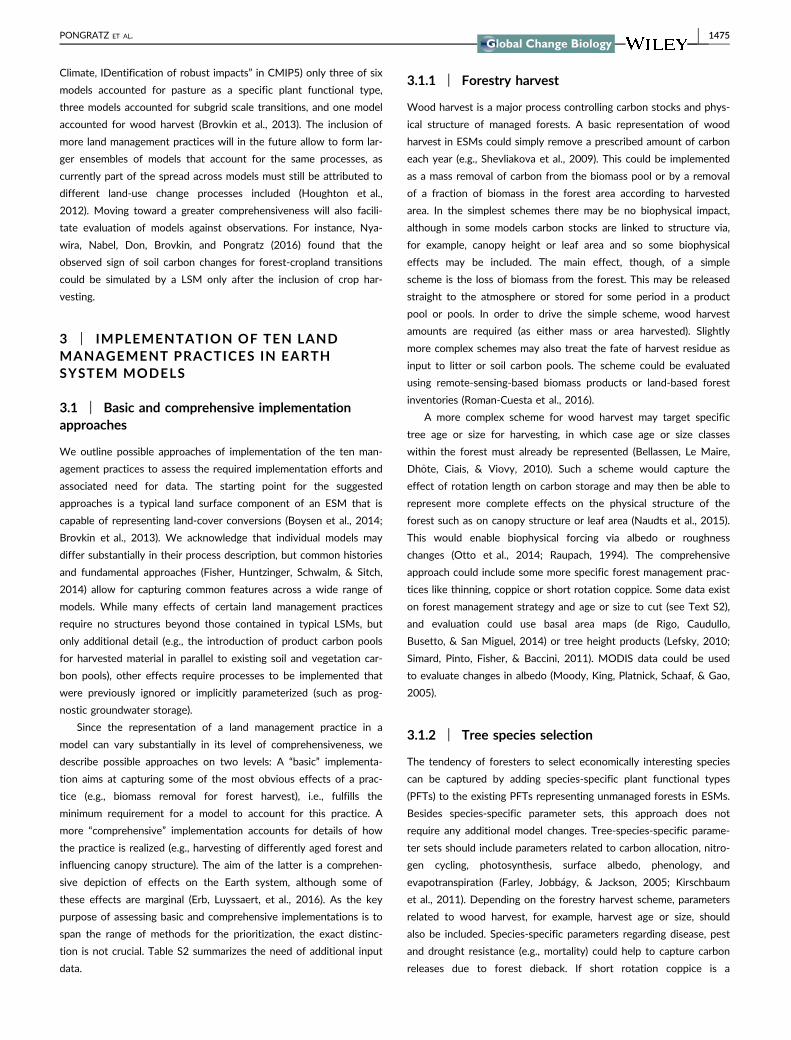
3.1.1 | Forestry harvest
Wood harvest is a major process controlling carbon stocks and phys-
ical structure of managed forests. A basic representation of wood
harvest in ESMs could simply remove a prescribed amount of carbon
each year (e.g., Shevliakova et al., 2009). This could be implemented
as a mass removal of carbon from the biomass pool or by a removal
of a fraction of biomass in the forest area according to harvested
area. In the simplest schemes there may be no biophysical impact,
although in some models carbon stocks are linked to structure via,
for example, canopy height or leaf area and so some biophysical
effects may be included. The main effect, though, of a simple
scheme is the loss of biomass from the forest. This may be released
straight to the atmosphere or stored for some period in a product
pool or pools. In order to drive the simple scheme, wood harvest
amounts are required (as either mass or area harvested). Slightly
more complex schemes may also treat the fate of harvest residue as
input to litter or soil carbon pools. The scheme could be evaluated
using remote-sensing-based biomass products or land-based forest
inventories (Roman-Cuesta et al., 2016).
A more complex scheme for wood harvest may target specific
tree age or size for harvesting, in which case age or size classes
within the forest must already be represented (Bellassen, Le Maire,
Dhote, Ciais, & Viovy, 2010). Such a scheme would capture the
effect of rotation length on carbon storage and may then be able to
represent more complete effects on the physical structure of the
forest such as on canopy structure or leaf area (Naudts et al., 2015).
This would enable biophysical forcing via albedo or roughness
changes (Otto et al., 2014; Raupach, 1994). The comprehensive
approach could include some more specific forest management prac-
tices like thinning, coppice or short rotation coppice. Some data exist
on forest management strategy and age or size to cut (see Text S2),
and evaluation could use basal area maps (de Rigo, Caudullo,
Busetto, & San Miguel, 2014) or tree height products (Lefsky, 2010;
Simard, Pinto, Fisher, & Baccini, 2011). MODIS data could be used
to evaluate changes in albedo (Moody, King, Platnick, Schaaf, & Gao,
2005).
3.1.2 | Tree species selection
The tendency of foresters to select economically interesting species
can be captured by adding species-specific plant functional types
(PFTs) to the existing PFTs representing unmanaged forests in ESMs.
Besides species-specific parameter sets, this approach does not
require any additional model changes. Tree-species-specific parame-
ter sets should include parameters related to carbon allocation, nitro-
gen cycling, photosynthesis, surface albedo, phenology, and
evapotranspiration (Farley, Jobb�agy, & Jackson, 2005; Kirschbaum
et al., 2011). Depending on the forestry harvest scheme, parameters
related to wood harvest, for example, harvest age or size, should
also be included. Species-specific parameters regarding disease, pest
and drought resistance (e.g., mortality) could help to capture carbon
releases due to forest dieback. If short rotation coppice is a
PONGRATZ ET AL. | 1475

management strategy a specific PFT could be dedicated to the spe-
cies that are usually used in these plantations. The species-specific
parameterization will affect all processes that are implemented at
the PFT level. If the model has a multilayer soil carbon and hydrol-
ogy scheme (see Section 3.1.7), species-specific root profiles will
help to capture species differences in water and nutrient uptake. For
the main European tree species parameter sets have already been
derived and applied (Hickler et al., 2012; Naudts et al., 2016).
A comprehensive implementation would include the representa-
tion of mixed-species stands. Representing species interactions in
mixed stands involves competition for light, water and nutrients (see
Pretzsch, Forrester, & R€otzer, 2015 for a review of model
approaches). Belowground competition can be captured when the
model includes multilayer soil carbon, nitrogen, phosphorus, and
hydrology schemes. Capturing light competition, however, would
require the replacement of the current “big leaf” approach of most
ESMs by a vertically explicit canopy structure with a multilayer radia-
tion scheme (Haverd et al., 2012; McGrath et al., 2016). The combi-
nation of a multilayer radiation and energy scheme enables
simulating emissions of biogenic volatile organic compounds (Sinde-
larova et al., 2014). Both basic and comprehensive implementations
require tree species distribution, whereas the comprehensive imple-
mentation also requires the distribution of mixed stands. The evalua-
tion approach can be similar to the one for forestry harvest (see
Section 3.1.1).
3.1.3 | Grazing and mowing harvest
While biophysical effects are found to be relatively weak, strong bio-
geochemical effects relate to this practice, in particular due to the
direct effect of carbon removal (Erb, Luyssaert, et al., 2016). The basic
implementation and evaluation of effects on carbon stocks are analo-
gous to removal of cropland biomass for crop harvest (e.g., Bondeau
et al., 2007; Lindeskog et al., 2013; Shevliakova et al., 2009), requiring
information on grazing intensity in terms of amount of biomass or frac-
tion of net primary production (NPP) removed. Effects are limited to
those related to altered carbon stocks. Yet, in reality grazing occurs
also on shrubby and woody vegetation (affecting low and high vegeta-
tion cover, the latter denoted “browsing”), so that additional informa-
tion is needed on type of vegetation to be grazed (ecosystem type and
the share of low and high vegetation affected) to overcome the cur-
rent common ESM assumption that all land used for grazing is grass-
land. Such data are scarcely available, adding to the existing
uncertainties (Fetzel et al., 2017). An important additional effect of
grazing and mowing harvest is the emission of methane from livestock,
which accounts for about 2/3 of total non-CO2 greenhouse-gas emis-
sions from the livestock sector (Herrero et al., 2013). Methane emis-
sions can be simulated by models of different complexity linking feed
intake to fermentation products (Chang et al., 2013; Thornton & Her-
rero, 2010) combined with estimates of number of livestock (FAO-
STAT, 2007), but the lack of information on dietary composition in
ESMs suggests to approximate this by external input on spatially vary-
ing fractions of methane emissions per unit biomass removal.
A more comprehensive implementation accounts for the return
of carbon and nutrients in manure and urine, which is important on
grazed lands, with consequences on methane and nitrous oxide
emissions (Davidson, 2009; Thornton & Herrero, 2010) and on plant
productivity by accelerated nutrient cycling (e.g., McNaughton,
Banyikwa, & McNaughton, 1997). While methane emissions from
manure are commonly quantified as fraction of enteric methane pro-
duction (Thornton & Herrero, 2010), the simulation of nutrient
effects on soil respiration, plant growth, and nitrogen-related emis-
sions requires a representation of the nitrogen cycle. Information on
which systems are grazed vs. mowed is needed to determine manure
input, but does not exist yet. Simulating changes in ecosystem struc-
ture due to selective grazing such as woody encroachment in semi-
arid regions, which affects both biogeochemical and biophysical
pathways, requires a complex competition scheme.
3.1.4 | Crop harvest and residue management
Reflecting crops’ purpose of providing food, feed, and fiber, the most
basic implementation just represents a removal of a fixed fraction of
biomass at a fixed date (Lindeskog et al., 2013; Shevliakova et al.,
2009) or an interception of a fixed fraction of productivity or litter
(Olofsson & Hickler, 2008). Removed carbon can be released to the
atmosphere under the assumption that consumption of harvested
products occurs within short time periods or be transferred to short-
lived soil/litter pools (Oleson et al., 2013; Reick, Raddatz, Brovkin, &
Gayler, 2013), such that product pools are dispensable. Conse-
quences of crop harvest are a reduction in vegetation biomass and
consequently soil carbon stocks, associated with emissions of CO2
to the atmosphere, and biogeophysical changes that are associated
with altered vegetation cover. The only required input is information
on the amount of biomass that is removed, in absolute terms or rela-
tive to standing biomass, although globally fixed rates of removal or
biomass left on site are found in model studies (Malyshev, Shevli-
akova, Stouffer, & Pacala, 2015; Stocker, Strassmann, & Joos, 2011).
Evaluation of such removal can be done via yield data (e.g., Food
and Agricultural Organization (FAO), 2007) after translating yield dry
mass into carbon stocks, and soil carbon chronosequences or paired-
site studies (e.g., Don, Schumacher, & Freibauer, 2011; Poeplau
et al., 2011).
More comprehensive implementations will put emphasis on plau-
sible harvest dates by fixing them to statistical information or crop
calendars or, in regions with seasonal climate, by interactively simu-
lating harvest dates in dependence on phenological state or climate
conditions (e.g., Bondeau et al., 2007; Oleson et al., 2013). Removal
of nutrients is simulated together with carbon, which requires partic-
ular attention to the magnitude and fate of residues, which return
part of the nutrients to the system (Kumar & Goh,1999). The out-
lined approach requires structural changes to the phenology scheme
to account for a harvest date, and nutrient cycles. Residual material
goes to the litter pools, which generally exist in models; introduction
of product pools would allow for accounting for noninstantaneous
emissions, for example, due to storage of bioenergy. Effects are
1476 | PONGRATZ ET AL.

changes to carbon and nutrient cycles as well as a more realistic
depiction of phenological consequences. Additional input data are
needed on fate of harvest and residues and its return to the field as
organic amendments. Additional opportunity for evaluation results
from the interactive simulation of harvest dates (Sacks, Deryng,
Foley, & Ramankutty, 2010).
3.1.5 | Crop species selection
The large variety in crop species can be captured by extending the
existing model PFTs with crop functional types representing the
most widespread agricultural plant traits (Bondeau et al., 2007). If
the model already includes crop PFTs, allowing it to treat crops dif-
ferently than natural vegetation (crop harvest, irrigation, N fertiliza-
tion, . . .), no additional structures are needed (Bondeau et al., 2007;
Lokupitiya et al., 2009; de Noblet-Ducoudr�e et al., 2004). The tar-
geted species-specific parameters are similar to the ones for tree
species selection (see Section 3.1.2); however, additional parameters
related to the development of yield-bearing organs can be included.
This approach should allow for capturing crop differences in yield,
soil organic matter accumulation, nitrogen and phosphorus uptake,
evapotranspiration, and phenology. The latter is important as it
includes crop-specific sowing dates, which can determine harvest
date and seasonal changes in albedo (Sacks & Kucharik, 2011). Simi-
lar to crop harvest (see Section 3.1.4), evaluation can be done
against yield data, and additionally against MODIS albedo and evap-
otranspiration (Loarie, Lobell, Asner, Mu, & Field, 2011).
The combination of the above described crop-specific parameter-
ization and the implementation of mixed stands (see comprehensive
implementation in Section 3.1.2.) would allow to simulate intercrop-
ping (i.e., concurrently growing multiple (crop) species to maximize
resource usage) and agroforestry (i.e., if one of the species is a tree)
(Brisson, Bussiere, Ozier-Lafontaine, Tournebize, & Sinoquet, 2004).
Agroforestry in different forms may represent an important form of
land management, but data are particularly scarce. A recent analysis
reveals that about 43% of cropland areas, measured as 1 km2 grid-
cells, had at least 10% tree cover in 2010 (Zomer et al., 2016). A
certain fraction of this tree cover consists of patches of cropland
interspersed with wood patches, but agroforestry may play a signifi-
cant role. Beside parameter sets for crop functional types, informa-
tion on crop type distribution and rotation schemes is needed.
3.1.6 | Irrigation and paddy rice
Alleviating the water stress on the vegetation to enhance productivity
brings about unintended biophysical and biogeochemical effects,
including changes in transpiration, soil albedo and greenhouse-gas
emissions (in particular methane and nitrous oxide) (Erb, Luyssaert,
et al., 2016). Most models distinguish between water availability in
the soil and the subsequent water status of the plant (e.g., Clark et al.,
2011; Krinner et al., 2005; Lawrence et al., 2011; Naudts et al., 2015;
Sitch et al., 2003). Hence, a basic implementation could eliminate or
reduce water stress by increasing soil moisture at the expense of
violating the mass balance closure (Boucher et al., 2004; Leng et al.,
2013; de Vrese, Hagemann, & Claussen, 2016). The magnitude of the
stress reduction could be prescribed or simulated based on the evapo-
transpirative demand of the atmosphere (Boucher et al., 2004; Leng
et al., 2013; de Vrese et al., 2016). This approach could simulate the
effects of irrigation on plant growth, transpiration, soil albedo (Brisson
et al., 2003) and other greenhouse-gas emissions (Kulshreshtha &
Junkins, 2001). The approach requires spatially explicit data on irriga-
tion area and fraction of water need fulfilled, as human use does not
always correspond to optimal water volume (D€oll, Fritsche, Eicker, &
Schmied, 2014), and could be evaluated in its effects against yield
statistics (e.g., Food and Agricultural Organization (FAO), 2007), remo-
tely sensed phenology (Ganguly, Friedl, Tan, Zhang, & Verma, 2010),
and greenhouse-gas inventories or inversions (Saunois et al., 2016;
Thompson et al., 2014).
If mass balance closure is aimed for, which is required for assess-
ments of water availability, the water used for irrigation should,
depending on the location, be taken from the simulated aquifers or
surface water stocks such as reservoirs and rivers (Gleeson, Wada,
Bierkens, & van Beek, 2012; Postel, Daily, & Ehrlich, 1996). This
approach is more data-demanding as the simulated water stocks will
need to be evaluated against ground-truth data. Spatially explicit data
on the land area equipped for irrigation and fraction of water need
fulfilled should be complemented by data on soil depth to simulate
the groundwater table as well as data on sources of extraction. In
addition to the evaluation data discussed for the basic approach, this
scheme could also be evaluated against statistics of river flow (e.g.,
Monk, Wood, Hannah, & Wilson, 2007), soil water content (Entekhabi
et al., 2010; Tapley, Bettadpur, Ries, Thompson, & Watkins, 2004),
and amount of water extracted for irrigation (Gleeson et al., 2012;
Postel et al., 1996). Note that we propose to use the amount of
extracted water for evaluation rather than for driving the model. This
proposition is justified by the fact that changes in aquifers are calcu-
lated from irrigation statistics. If irrigation statistics are prescribed, the
simulated changes in aquifers can no longer be used to evaluate this
aspect of model performance. A consequence of this proposition is
that irrigation demand will need to be calculated by considering plant
physiology in combination with the atmospheric condition.
A comprehensive implementation of irrigation would also
account for paddy rice. Paddy rice has different drivers and effects
from irrigation of other crops. The aim is not alleviation of water
stress but weed and pest control. The primary impact is via methane
emissions. Surface biophysics are also altered in terms of evaporative
ability and albedo. To capture emissions of other greenhouse gases,
which are particularly important for paddy rice (Wassmann et al.,
2000), models should include methane production as well as an N
cycle which can adapt to anaerobic conditions through reduced
decomposition and enhanced denitrification (Kraus et al., 2015).
3.1.7 | Artificial wetland drainage
Wetlands cover about 4% of the land surface but store about one-
third of the soil organic carbon, mainly in peatlands (Aselmann &
PONGRATZ ET AL. | 1477

Crutzen, 1989). Even in the absence of a representation of peat-
lands, a basic implementation of drainage is feasible in models
including a multilayer hydrology by removing water from the lower
soil layers and adding it to the run-off (in addition to the gravita-
tional drainage commonly represented in ESMs). We are not aware
of ESMs that implemented wetland drainage.
A comprehensive approach would require that models distinguish
between mineral and organic soils (Letts, Roulet, Comer, Skarupa, &
Verseghy, 2000/2010; Wisser, Marchenko, Talbot, Treat, & Frolking,
2011) and simulate a groundwater table in its multilayer soil water
scheme. Drainage could still be represented by removing water from
the soil layer that corresponds to the typical depth of a drainage
channel. The effects of a reduced soil water content on greenhouse-
gas emissions and transpiration can then be simulated by the exist-
ing process representation in the model. Both basic and comprehen-
sive implementations require knowledge of the extent of drainage
and drainage depth and an adequate routing scheme to simulate the
lateral transport. Most often drainage is followed by a land-cover
conversion, which is expected to cause the main biogeochemical and
biophysical effects. This land-cover conversion will need to be pre-
scribed unless its socioeconomic drivers are sufficiently understood.
The validation of drainage would thus require to separate between
the effects of drainage and the subsequent land-cover change. We
could not identify datasets which at present would support such a
validation.
3.1.8 | Nitrogen and phosphorous fertilization ofcropland and grazing land
The biogeochemical effect of N fertilization is large and well-docu-
mented (Erb, Luyssaert, et al., 2016), explaining our suggestion to
implement the key N cycling processes in both basic and complex
approaches. N cycle processes not related to land management, i.e.,
representation of N inputs from atmospheric deposition and biologi-
cal fixation, and ecosystem losses through leaching and microbial
emissions, need to be extended to account for input from fertilizer
application. In a basic representation, N uptake can be a function of
demand and availability, where the demand is determined by assum-
ing a fixed C/N ratio in plant and soil compartments, i.e., if the
amount of carbon in the pool increases, N increases accordingly (Goll
et al., 2012; Thornton, Lamarque, Rosenbloom, & Mahowald, 2007).
In this approach, N limitation is relaxed and biomass production
increased as a result of N fertilization, but plants are not allowed to
optimize their C/N ratio (Haxeltine & Prentice, 1996), possibly lead-
ing to an overestimation of N limitation. In the basic approach micro-
bial N emissions consist of nitrification and denitrification which can
be a function of mineral nitrogen concentration, soil moisture, tem-
perature, pH, and carbon availability (Butterbach-Bahl, Baggs, Dan-
nenmann, Kiese, & Zechmeister-Boltenstern, 2013).
In the comprehensive implementation N concentration in plant
and soil are simulated dynamically, and therefore carbon fluxes
respond to the N status (Xu-Ri & Prentice, 2008; Zaehle & Friend,
2010). In this approach, N uptake can be determined according to
Michaelis–Menten kinetics, proportional to fine root biomass or sur-
face area, N availability, and plant N status. Additional model devel-
opments could include N-dependent allocation (shift toward
belowground carbon to improve N status, Smith et al., 2014), plant–
rhizosphere interactions mediated by carbon export (Stocker et al.,
2016), and nitrification and denitrification based on microbial dynam-
ics (Butterbach-Bahl et al., 2013). The comprehensive implementa-
tion should also capture potential biophysical effects of N
fertilization through increased leaf area.
Although the effect of fertilization by other nutrients (in particu-
lar phosphorus (P) and potassium (K)) on climate is much smaller
than for N fertilizer, they could be included if the model includes
their respective biogeochemical cycle (e.g., Goll et al. (2012) for
phosphorus). Phosphorus in particular plays a key role in the tropics.
The required input for both basic and comprehensive implemen-
tations consists of spatially explicit information on the area and
amount of applied N (and P, K)-fertilizer. Additional information
could be the timing of the nutrient fertilization. The scheme can be
evaluated against yield data (e.g., Food and Agricultural Organization
(FAO), 2007), soil carbon (e.g., Don et al., 2011; Poeplau et al.,
2011) and N concentration in rivers (Nevison, Hess, Riddick, & Ward,
2016).
3.1.9 | Tillage
The multitude of soil processes affected by tillage, which are not
well understood (Erb, Luyssaert, et al., 2016), suggest a simple
parameterization as basic form of implementation in models (Chats-
kikh, Hansen, Olesen, & Petersen, 2009). Observation-based rate
modifier terms for reduced tillage and no-till management for soil
respiratory fluxes allow capturing effects on soil carbon stocks and
CO2 fluxes (Pugh et al., 2015). The only required input is knowledge
of the area under tillage and possibly the form of tillage for specific
parameterizations. Soil carbon chronosequences or paired sites can
be used for evaluation (e.g., Don et al., 2011; Poeplau et al., 2011) if
they have not entered the parameterization.
A process-based representation of tillage effects requires repre-
senting vertical layers of soil, with the top layers exchanging carbon
and water due to tillage, which leads to different conditions for
decomposition. Therefore, the representation of tillage would bene-
fit from a microbial-based decomposition instead of the first-order
decomposition that is generally used in ESMs but lacks microbial
control (Todd-Brown, Hopkins, Kivlin, Talbot, & Allison, 2012; Xena-
kis & Williams, 2014). While many LSMs represent vertical soil lay-
ers for water (e.g., De Rosnay, Polcher, Bruen, & Laval, 2002;
Hagemann & Stacke, 2015; Oleson et al., 2013), layered soil carbon
schemes (e.g., Braakhekke et al., 2011; Koven et al., 2013) are less
commonly applied. The top-soil mixing allows for representing
altered soil respiration fluxes and, depending on the capabilities of
the model’s soil scheme, other greenhouse-gas emissions. Altered
soil moisture further influences plant growth, surface water fluxes,
and soil albedo. Effects of stubble on albedo can partly be captured
by distinguishing between transfer of on-site residues to soil/litter
1478 | PONGRATZ ET AL.

pools in the case of tillage (see description of crop harvest and resi-
due management) and onsite residues left in the biomass pools for
no-till, or be parameterized, as can be effects of mulch on evapora-
tion (Davin et al., 2014). This more comprehensive implementation,
however, requires additional input concerning depth of tillage and
possibly seasonal timing. Observational data on soil moisture and
albedo for till vs. no-till locations can be used for evaluation (e.g.,
Davin et al., 2014) in addition to carbon stock chronosequences or
paired sites.
3.1.10 | Fire as management tool
Fire has multiple uses in agriculture, for example, to burn crop resi-
dues or manage grazing lands. In inhabited fire-prone areas, pre-
scribed burning is used to prevent wildfires and if these preventive
measures fail, fire suppression is expected to avoid losses. In a basic
biogeochemistry-oriented implementation, a fraction of the litter and
standing biomass—after harvest—should be put back into the atmo-
sphere as burn gases (Van der Werf et al., 2010). The burn gases
could distinguish between different carbon and nitrogen compounds
by making use of generic emission factors (Akagi et al., 2011).
A comprehensive implementation accounting for both the bio-
physical and the biogeochemical effects of fire management (includ-
ing potentially emissions relevant to wider atmospheric composition
interactions such as biomass burning aerosols, methane and carbon
monoxide) requires that the vegetation structure is accounted for
(Randerson et al., 2006). Where fire management is applied in wood-
land savannas, this may require structural model developments that
enable mixed PFTs (see implementation of mixed stands in Section
3.1.2), such that trees and grasses compete for the same water,
nutrient, and light resources (Saito et al., 2014; Scheiter & Higgins,
2009; Simioni, Le Roux, Gignoux, & Sinoquet, 2000). In forests, the
vegetation structure needs to represent a canopy structure. Preven-
tive fires will then remove part of the litter and the fuel ladders that
connect the litter layer with the top canopy through the crowns of
the small trees (Scherer, DAmato, Kern, Palik, & Russell, 2016). The
chemical composition and dimensions of the biomass as well as the
fire characteristics can be used to adjust the emission factors of the
burn gases in terms of their carbon and nitrogen compounds (Lobert
et al., 1990; Surawski, Sullivan, Meyer, Roxburgh, & Polglase, 2015;
Urbanski, 2013). Both the basic and comprehensive approaches
require a spatially explicit driver that prescribes the areas where fire
is used as a management tool in agriculture and forestry.
The implementation of fire suppression builds on the functional-
ity required to simulate wildfires (Arora & Boer, 2005; Mann et al.,
2016; Thonicke et al., 2010). When a wildfire is ignited and the
resources for fire suppression are available, a fire suppression mod-
ule should stop the fire before the natural conditions for burning
would stop the fire. A fire suppression module could thus be driven
by regional data on the capacity to fight fires as well as the size of
the fire, the population density and the property value in the vicinity
of the fire to set decisions rules on where to fight wildfires.
3.2 | Structural dependencies
The implementation of land management practices might require
that new structures and processes are added to the model architec-
ture. In Figure 4 we collect the new structures and processes
required for the implementation described in Section 3.1 (in paren-
theses the total number for basic/comprehensive implementation
approaches). The degree of these required changes differs largely
between land management practices. For example, tree species
selection requires a small, and wetland drainage and fire manage-
ment a large number of new processes and structures to be imple-
mented.
The required changes introduce dependencies between the land
management practices when they are implemented in a comprehen-
sive way, as many processes and structures form basis for more than
Crop species selection (1/2)
Fire management (1/5)
Forestry harvest (1/3) Tree species selection (0/2)
Irrigation & paddy rice (0/3) Wetland drainage (1/5)
Grazing & mowing (1/3) Crop harvest & residues (0/3)
Tillage (0/3) Fertilization (1/4)
F IGURE 4 Dependencies of processesand structures required for thecomprehensive implementation of the tendiscussed land management practices.Asterisks indicate which processes andstructures are also needed for a basicimplementation. The number of processesand structures required for a basic andcomprehensive implementation areindicated for each practice in parentheses.Processes and structures for both basicand comprehensive implementation arecollected from the description ofimplementation of land managementpractices in Section 3.1
PONGRATZ ET AL. | 1479

one practice. Figure 4 shows the interrelation between processes
and structures required for the implementation of our ten land man-
agement practices. Some structures emerge as being essential in that
they form basis for many practices, such as the nitrogen cycle for a
more comprehensive implementation, while others are specific to
individual practices, such as age structure (Figure 4). Note that the
most essential structures of a comprehensive implementation include
the nitrogen cycle, canopy structure, mixed-species stands, and rep-
resentations of methane, most of which go far beyond an extension
of existing structures. Considerations of prioritization thus may not
just include the number and complexity of processes and structures
required by individual land management practices, but also synergies
that practices provide in sharing key structures with other practices.
For example, all new structures required for tree species selection
would already be available following an implementation of fire man-
agement or forestry harvest plus crop species selection; similarly irri-
gation and paddy rice could use the structures provided by
implementation of wetland drainage.
4 | MATCHING MODEL REQUIREMENTSWITH AVAILABLE DATA
4.1 | Data requirements and availability
Each land management practice comes with certain additional vari-
ables that need to be prescribed from external data (summarized
from Section 3.1 in Table S2). Most information is required globally
and in a spatially explicit way and describes in particular the extent
and intensity of the practices, but implementing crop and tree spe-
cies selection would also require extending the existing parameter
sets. Land management has substantially changed over history, and
modeling land-use change effects involves simulations covering a
decadal to centennial timescale to capture in particular delayed bio-
geochemical fluxes and slow feedback responses in the Earth sys-
tem. Therefore, input datasets need to cover these timescales. Yet,
observational data are useful for model evaluation even when avail-
able only for certain regions or time periods.
Timescales of decades to centuries imply that deriving informa-
tion on the input variables from Earth observation is often not suf-
ficient—it needs to be possible to reconstruct the same variable
from statistical or inventory data to capture time periods prior to
the satellite era (e.g., statistics on agricultural area by the Food and
Agricultural Organization, statistics on wood production by FAO’s
Global Forest Resources Assessments, forest inventories). Further-
more, ESMs are frequently used to project anthropogenic effects,
including land-use change, into the future (e.g., Brovkin et al.,
2013); the same variable thus needs to be available, from global
land system or integrated assessment modeling, for future scenar-
ios. For some land-use conversions and certain land management
practices a harmonization of historical, Earth observation, and IAM
data has been performed for CMIP5 (Hurtt et al., 2011) and is cur-
rently extended for CMIP6, but covers only a subset of the vari-
ables identified as essential input in Section 3.1. Discrepancies
between priorities of IAMs and ESMs may therefore limit ESM
applications for future management.
We assess the availability of observational datasets as input vari-
ables or parameters as required by the implementation outlined in
Section 3.1. It should be noted that few of these datasets are direct
observations—many are processed data products relying on addi-
tional assumptions, including partly even process-based modeling
(see Text S2). Our assessment of data availability aims at simulations
for the historical time period (e.g., for simulations covering the indus-
trial era) and includes aspects of data quality and spatial and tempo-
ral coverage (Table S2 and Text S2). Our assessment reveals that
data availability differs vastly across the ten land management prac-
tices. Good data availability exists for cropland management prac-
tices where mostly area information is required (as for basic
implementations of crop species selection, fertilization, tillage). Poor
data availability is found for forestry harvest, grazing and mowing
harvest, artificial wetland drainage, and tillage when the comprehen-
sive assessment requires additional data streams. Partly this may be
attributable to complications in separating natural from managed
processes in Earth observations.
4.2 | Model-data gaps and opportunities
The criteria for prioritization discussed in the introduction refer to
three broad categories: (1) the importance of a land management
practice for the Earth system as indicated by spatial extent and
strength of biogeochemical and biogeophysical effects, (2) the possi-
bility of technical implementation as indicated by the process under-
standing and ease of implementation, and (3) data availability. The
following conclusions can be drawn by contrasting these three
aspects (Figure 5):
(1). “Low-hanging fruits” for modeling a land management practice,
where all three aspects are well covered, emerge for a basic
implementation approach. Crop harvest and residue manage-
ment, nitrogen fertilization, and (with some more restrictions on
data availability but larger spatial extent) forestry harvest are all
important for the Earth system, possible to implement in current
ESMs, and provide good data availability (Figure 5a). However,
for all three practices the ease of implementation and data
availability dramatically drop for a comprehensive implementa-
tion (Figure 5b).
(2). For some land management practices data availability and robust-
ness is the key obstacle for simulating their effects in ESMs. Most
notably, data availability is poor for grazing and mowing harvest,
which is important for the Earth system and rather easy to imple-
ment in current ESMs. Here, a substantial number of variables
needs to be provided with external data and quality of the indi-
vidual datasets is poor (Figure 5a and Text S2). The problem
arises both for the basic and comprehensive implementation,
interfering with modeling groups’ plans of moving toward repre-
sentation of grazing processes in their models (Figure 2). Data
availability is poor also for artificial wetland drainage and fire as
1480 | PONGRATZ ET AL.

management tool, but implementation for these practices is
equally hindered by the lack of process understanding. Data avail-
ability becomes the limiting factor for many land management
practices for a comprehensive implementation (Figure 5b).
(3). A call for more research on process understanding was voiced
by Erb, Luyssaert, et al. (2016) for crop species selection, tillage,
artificial wetland drainage, and fire as management tool. Our
analysis shows that for the first two, process understanding is
indeed the major obstacle, as the available structures of current
ESMs are capable of catching the basic effects of crop species
selection and tillage and data availability is good. Simulation of
the latter two is also hindered by data availability.
(4). Existing model structures of current ESMs are largely sufficient
to capture key effects of land management, but major extension
of current model structures are required to capture both bio-
geophysical and biogeochemical effects comprehensively.
Our prioritization results are partly reflected in model develop-
ment: Coincidence of importance, modeling ease, and data availabil-
ity for a basic implementation of crop harvest and residue
management, which only relies on removal of biomass, indeed is one
of the most common land management features in the current gen-
eration of models (Figure 2). That most models move toward the
inclusion of the nitrogen cycle (Figure 2) coincides with nitrogen
Forestry harvest Tree species Grazing Crop harvest Crop species
Irrigation Drainage Fertilization Tillage Fire
Forestry harvest Tree species Grazing Crop harvest Crop species
Irrigation Drainage Fertilization Tillage Fire
(a)
(b)
(c)
F IGURE 5 Matching importance for theEarth system, possibility of technicalimplementation in ESMs, and dataavailability for the ten land managementpractices. The legend in panel c explainsthe criteria: Importance for the Earthsystem is depicted by spatial extent andcombined strength of biogeophysical andbiogeochemical effects (from Erb,Luyssaert, et al., 2016 Figures 2 and 3,resp.); possibility of technicalimplementation in ESMs is depicted byprocess understanding (classified as eitherpoor or advanced by Erb, Luyssaert, et al.,2016; table 2) and ease of implementation(represented by number of structuresrequired for the implementationapproaches of Section 3.1, see alsoFigure 4); data availability is based on thedescription and scoring of the individualdatasets required for implementation inESMs as described in Table S2 and TextS2. Panel a refers to a “basic”implementation, b to a “comprehensive”one, meaning that ease of implementationand data availability differ between a andb. All values are scaled to maximum = 1.For data availability, the scorings for theindividual variables/datasets areaggregated to one single value as (N * 3–SUM(Si))/(N * 3–1), where N is the numberof required datasets (maximum of basicand comprehensive implementation foreach land management practice) and Si isthe score of the data availability for eachdataset i required for the basic andcomprehensive implementation,respectively, with 1 = good, 2 = medium,3 = poor data availability
PONGRATZ ET AL. | 1481

fertilization being recognized as important and, despite its own com-
plexity, requiring only nutrient-related structures (Figure 4). Grazing
and mowing harvest, which requires many additional structures and
processes, is left only to the third generation of ESMs, requiring
future progress on data availability. A good observational basis may
also have been a driver of past model development. For example,
the availability of large databases such as from the eddy covariance
network Fluxnet (Baldocchi et al., 2001) or the global plant trait
database (Kattge et al., 2011) pushed the carbon cycle development
in LSMs; the wide inclusion of wood harvest (Figure 2) occurred as
part of the development for CMIP5, which provided gridded wood
harvest information (Hurtt et al., 2011). On the other hand, new sci-
entific questions in the ESM community fostered specific develop-
ment of datasets, such as the first global reconstructions of some
historical land-use and land-cover conversions (Kaplan, Krumhardt, &
Zimmermann, 2009; Klein Goldewijk, 2001; Pongratz, Reick, Raddatz,
& Claussen, 2008; Ramankutty & Foley, 1999).
5 | CONCLUSIONS
As the applications of Earth system models move from general cli-
mate projections toward questions of mitigation and adaptation
(Lawrence et al., 2016) the more comprehensive representation of
land management practices becomes crucial. A corresponding trend
toward a more comprehensive representation of land use generally,
and land management in particular, in ESMs is clearly discernable.
This development can be guided by a prioritization of land manage-
ment practices based on their importance for the Earth system, the
possibility of technical implementation in the model, and data avail-
ability. Our review of these aspects reveals some “low-hanging
fruits” such as a basic implementation of crop harvest and residue
management, nitrogen fertilization, and forestry harvest, where exist-
ing model structures are mostly sufficient to capture certain key
effects on the Earth system and the required additional input vari-
ables can be derived from observational or statistical datasets.
Our review also pinpoints the need for additional research in
specific communities: the implementation, even in a simple form, of
the most extensive land management practice—grazing and mowing
harvest—is severely hampered by the lack of high-quality data, and
data availability reveals substantial gaps for almost all of the land
management practices assessed in this study when the aim is to cap-
ture their effects in a comprehensive way. A lack of process under-
standing is complicating implementation of practices that otherwise
can be easily linked to existing model structures and datasets (such
as crop species selection and tillage for a basic implementation).
Finally, while some key effects of most land management practices
can be captured without major extension of ESMs to additional struc-
tures, major model development will be the challenge for a compre-
hensive representation of biogeophysical and biogeochemical effects.
Extending ESMs to a more comprehensive representation of
land management effects will in the near future lead to model
divergence as the planned paths of model development and
prioritization differ between modeling groups. It will, however,
allow for a more accurate description of the human impact on the
Earth system as long as the multimodel assessments required to
overcome model biases are based on selecting models with compa-
rable representation of land management practices. A multitude of
observational datasets can be included for evaluation purposes that
were not meaningful in earlier-generation models, because earlier
models lacked a detailed representation of vegetation processes
that are relevant for land management practices and captured by
Earth observations. To achieve a comprehensive inclusion of land
management in ESMs a continuous collaboration of the modeling
community, Earth observation community, as well as land system
science is required beyond the identification of challenges and
opportunities provided by this study.
ACKNOWLEDGEMENTS
We thank the various modeling groups providing insight into their
modeling plans as depicted in Figures 2 and 3. The authors gratefully
acknowledge the support of the International Space Science Institute
(Bern) that sponsored the team on “Integrating Earth Observation
data and the description of land management practices into global
carbon cycle models” (A.J. Dolman). JP and KN were supported by
the German Research Foundation’s Emmy Noether Program (PO
1751/1-1). PM is Research Associate with the Fonds de la
Recherche Scientifique (F.R.S.-FNRS/Belgium), which supports this
work. CDJ was supported by the Joint UK BEIS/Defra Met Office
Hadley Centre Climate Programme (GA01101) and EU H2020 pro-
ject CRESCENDO (grant no. 641816) and FP7 LUC4C (grant no.
603542). AJD recognizes the support of the NESSC Netherlands
Earth System Sensitivity Centre. MH was supported by the Euro-
pean Space Agency Land Cover CCI Project and the ESA GOFC-
GOLD project office. KHE acknowledges funding from ERC-Stg
263522 LUISE and H2020 640176 BACI. This work contributes to
the Global Land Programme glp.earth. Primary data used in the anal-
ysis are archived by the Max Planck Institute for Meteorology and
can be obtained by contacting [email protected].
ORCID
Julia Pongratz http://orcid.org/0000-0003-0372-3960
Han Dolman http://orcid.org/0000-0003-0099-0457
Axel Don http://orcid.org/0000-0001-7046-3332
Richard Fuchs http://orcid.org/0000-0003-3830-1274
Sebastiaan Luyssaert http://orcid.org/0000-0003-1121-1869
REFERENCES
Akagi, S., Yokelson, R. J., Wiedinmyer, C., Alvarado, M., Reid, J., Karl, T.,
. . . Wennberg, P. (2011). Emission factors for open and domestic bio-
mass burning for use in atmospheric models. Atmospheric Chemistry
and Physics, 11(9), 4039–4072. https://doi.org/10.5194/acp-11-
4039-2011
1482 | PONGRATZ ET AL.

Arneth, A., Sitch, S., Pongratz, J., Stocker, B., Ciais, P., Poulter, B., . . .
Zaehle, S. (2017). Historical carbon dioxide emissions caused by land-
use changes are possibly larger than assumed. Nature Geoscience, 10,
79–84. https://doi.org/10.1038/ngeo2882
Arora, V. K., & Boer, G. J. (2005). A parameterization of leaf phenology
for the terrestrial ecosystem component of climate models. Global
Change Biology, 11(1), 39–59. https://doi.org/10.1111/j.1365-2486.
2004.00890.x
Aselmann, I., & Crutzen, P. (1989). Global distribution of natural freshwa-
ter wetlands and rice paddies, their net primary productivity, season-
ality and possible methane emissions. Journal of Atmospheric
Chemistry, 8(4), 307–358. https://doi.org/10.1007/BF00052709
Baldocchi, D., Falge, E., Gu, L., Olson, R., Hollinger, D., Running, S., . . .
Fuentes, J. (2001). FLUXNET: A new tool to study the temporal and
spatial variability of ecosystem–scale carbon dioxide, water vapor,
and energy flux densities. Bulletin of the American Meteorological Soci-
ety, 82(11), 2415–2434. https://doi.org/10.1175/1520-0477(2001)
082<2415:FANTTS>2.3.CO;2
Bellassen, V., Le Maire, G., Dhote, J., Ciais, P., & Viovy, N. (2010). Model-
ling forest management within a global vegetation model — part 1:
Model structure and general behaviour. Ecological Modelling, 221(20),
2458–2474. https://doi.org/10.1016/j.ecolmodel.2010.07.008
Bondeau, A., Smith, P., Zaehle, S., Schaphoff, S., Lucht, W., Cramer,
W., . . . Smith, B. (2007). Modelling the role of agriculture for the
20th century global terrestrial carbon balance. Global Change Biol-
ogy, 13(3), 679–706. https://doi.org/10.1111/j.1365-2486.2006.
01305.x
Boucher, O., Myhre, G., & Myhre, A. (2004). Direct human influence of
irrigation on atmospheric water vapour and climate. Climate Dynam-
ics, 22(6–7), 597–603. https://doi.org/10.1007/s00382-004-0402-4
Boysen, L., Brovkin, V., Arora, V., Cadule, P., de Noblet-Ducoudr�e, N.,
Kato, E., . . . Gayler, V. (2014). Global and regional effects of land-use
change on climate in 21st century simulations with interactive carbon
cycle. Earth System Dynamics, 5(2), 309–319. https://doi.org/10.
5194/esd-5-309-2014
Braakhekke, M., Beer, C., Hoosbeek, M., Reichstein, M., Kruijt, B.,
Schrumpf, M., & Kabat, P. (2011). SOMPROF: A vertically explicit soil
organic matter model. Ecological Modelling, 222, 1712–1730.
https://doi.org/10.1016/j.ecolmodel.2011.02.015
Brisson, N., Bussiere, F., Ozier-Lafontaine, H., Tournebize, R., & Sinoquet,
H. (2004). Adaptation of the crop model STICS to intercropping. The-
oretical basis and parameterisation. Agronomie, 24(6–7), 409–421.
https://doi.org/10.1051/agro:2004031
Brisson, N., Gary, C., Justes, E., Roche, R., Mary, B., Ripoche, D., . . . Bus-
si�ere, F. (2003). An overview of the crop model STICS. European Jour-
nal of agronomy, 18(3), 309–332. https://doi.org/10.1016/S1161-
0301(02)00110-7
Brovkin, V., Boysen, L., Arora, V., Boisier, J., Cadule, P., Chini, L., . . .
Weiss, M. (2013). Effect of anthropogenic land-use and land-cover
changes on climate and land carbon storage in CMIP5 projections for
the twenty-first century. Journal of Climate, 26(18), 6859–6881.
https://doi.org/10.1175/JCLI-D-12-00623.1
Butterbach-Bahl, K., Baggs, E. M., Dannenmann, M., Kiese, R., &
Zechmeister- Boltenstern, S. (2013). Nitrous oxide emissions from
soils: How well do we understand the processes and their controls?
Philosophical transactions of the Royal Society of London. Series B, Bio-
logical Sciences, 368(1621), 20130122. https://doi.org/10.1098/rstb.
2013.0122
Chang, J., Viovy, N., Vuichard, N., Ciais, P., Wang, T., Cozic, A., . . . Sous-
sana, J. F. (2013). Incorporating grassland management in ORCHIDEE:
model description and evaluation at 11 eddy-covariance sites in Eur-
ope. Geoscientific Model Development, 6(6), 2165–2181. https://doi.
org/10.5194/gmd-6-2165-2013
Chatskikh, D., Hansen, S., Olesen, J. E., & Petersen, B. M. (2009). A sim-
plified modelling approach for quantifying tillage effects on soil
carbon stocks. European Journal of Soil Science, 60(6), 924–934.
https://doi.org/10.1111/j.1365-2389.2009.01185.x
Clark, D., Mercado, L., Sitch, S., Jones, C., Gedney, N., Best, M., . . . Bou-
cher, O. (2011). The Joint UK Land Environment Simulator (JULES),
model description-Part 2: carbon fluxes and vegetation dynamics.
Geoscientific Model Development, 4(3), 701. https://doi.org/10.5194/
gmd-4-701-2011
Collins, W. D., Craig, A. P., Truesdale, J. E., Di Vittorio, A., Jones, A. D., Bond-
Lamberty, B., . . . Patel, P. (2015). The integrated earth system model
version 1: Formulation and functionality. Geoscientific Model Develop-
ment, 8(7), 2203–2219. https://doi.org/10.5194/gmd-8-2203-2015
Davidson, E. A. (2009). The contribution of manure and fertilizer nitrogen
to atmospheric nitrous oxide since 1860. Nature Geoscience, 2(9),
659–662. https://doi.org/10.1038/ngeo608
Davin, E. L., Seneviratne, S. I., Ciais, P., Olioso, A., & Wang, T. (2014).
Preferential cooling of hot extremes from cropland albedo manage-
ment. Proceedings of the National Academy of Sciences of the United
States of America, 111(27), 9757–9761. https://doi.org/10.1073/pna
s.1317323111
De Rosnay, P., Polcher, J., Bruen, M., & Laval, K. (2002). Impact of a
physically based soil water flow and soil-plant interaction representa-
tion for modeling large-scale land surface processes. Journal of Geo-
physical Research: Atmospheres, 107(D11).
D€oll, P., Fritsche, M., Eicker, A., & Schmied, H. M. (2014). Seasonal water
storage variations as impacted by water abstractions: Comparing the
output of a global hydrological model with grace and gps observa-
tions. Surveys in Geophysics, 35(6), 1311–1331. https://doi.org/10.
1007/s10712-014-9282-2
Don, A., Schumacher, J., & Freibauer, A. (2011). Impact of tropical land-
use change on soil organic carbon stocks–a meta-analysis. Global
Change Biology, 17(4), 1658–1670. https://doi.org/10.1111/j.1365-
2486.2010.02336.x
Eastman, J. L., Coughenour, M. B., & Pielke, R. A. Sr (2001). Does grazing
affect regional climate? Journal of Hydrometeorology, 2(3), 243–253.
https://doi.org/10.1175/1525-7541(2001)002<0243:DGARC>2.
0.CO;2
Entekhabi, D., Njoku, E. G., O’Neill, P. E., Kellogg, K. H., Crow, W. T.,
Edelstein, W. N., . . . Kimball, J. (2010). The soil moisture active pas-
sive (SMAP) mission. Proceedings of the IEEE, 98(5), 704–716.
https://doi.org/10.1109/JPROC.2010.2043918
Erb, K.-H., Haberl, H., & Plutzar, C. (2012). Dependency of global primary
bioenergy crop potentials in 2050 on food systems, yields, biodiver-
sity conservation and political stability. Energy Policy, 47, 260–269.
https://doi.org/10.1016/j.enpol.2012.04.066
Erb, K.-H., Lauk, C., Kastner, T., Mayer, A., Theurl, M. C., & Haberl, H.
(2016). Exploring the biophysical option space for feeding the world
without deforestation. Nature communications, 7, 1–9.
Erb, K.-H., Luyssaert, S., Meyfroidt, P., Pongratz, J., Don, A., & Kloster, S.,
. . . Dolman, A. J. (2016). Land management: Data availability and pro-
cess understanding for global change studies. Global Change Biology,
23, 512–533.
Farley, K. A., Jobb�agy, E. G., & Jackson, R. B. (2005). Effects of afforesta-
tion on water yield: A global synthesis with implications for policy.
Global Change Biology, 11(10), 1565–1576. https://doi.org/10.1111/j.
1365-2486.2005.01011.x
Fetzel, T., Havlik, P., Herrero, M., Kaplan, J., Kastner, T., Kroisleitner, C.,
. . . Erb, K. H. (2017). Quantification of uncertainties in global grazing
systems assessments. Global Biogeochemical Cycles, 31, 1089–1102.
https://doi.org/10.1002/2016GB005601
Fisher, J. B., Huntzinger, D. N., Schwalm, C. R., & Sitch, S. (2014). Model-
ing the terrestrial biosphere. Annual Review of Environment and
Resources, 39, 91–123. https://doi.org/10.1146/annurev-environ-
012913-093456
Flato, G., Marotzke, J., Abiodun, B., Braconnot, P., Chou, S. C., & Collins,
W. J., . . . others (2013). Evaluation of Climate Models. In: Climate
PONGRATZ ET AL. | 1483

Change 2013: The Physical Science Basis. Contribution of Working
Group I to the Fifth Assessment Report of the Intergovernmental
Panel on Climate Change. Climate Change 2013, 5, 741–866.
Foley, J. A., Ramankutty, N., Brauman, K. A., Cassidy, E. S., Gerber, J. S.,
Johnston, M., . . . Balzer, C. (2011). Solutions for a cultivated planet.
Nature, 478(7369), 337–342. https://doi.org/10.1038/nature10452
Food and Agricultural Organization (FAO). (2007). FAOSTAT: Land use.
FAO Statistics Division.
Ganguly, S., Friedl, M. A., Tan, B., Zhang, X., & Verma, M. (2010). Land
surface phenology from MODIS: Characterization of the collection 5
global land cover dynamics product. Remote Sensing of Environment,
114(8), 1805–1816. https://doi.org/10.1016/j.rse.2010.04.005
Gleeson, T., Wada, Y., Bierkens, M. F., & van Beek, L. P. (2012). Water
balance of global aquifers revealed by groundwater footprint. Nature,
488(7410), 197–200. https://doi.org/10.1038/nature11295
Goll, D., Brovkin, V., Parida, B., Reick, C. H., Kattge, J., Reich, P., . . . Nii-
nemets, €U. (2012). Nutrient limitation reduces land carbon uptake in
simulations with a model of combined carbon, nitrogen and phospho-
rus cycling. Biogeosciences, 9, 3547–3569. https://doi.org/10.5194/
bg-9-3547-2012
Haberl, H., Erb, K., Krausmann, F., Gaube, V., Bondeau, A., Plutzar, C., . . .
Fischer-Kowalski, M. (2007). Quantifying and mapping the human
appropriation of net primary production in earth’s terrestrial ecosys-
tems. Proceedings of the National Academy of Sciences of the United
States of America, 104(31), 12942–12947. https://doi.org/10.1073/
pnas.0704243104
Hagemann, S., & Stacke, T. (2015). Impact of the soil hydrology scheme
on simulated soil moisture memory. Climate Dynamics, 44(7–8),
1731–1750. https://doi.org/10.1007/s00382-014-2221-6
Haverd, V., Lovell, J., Cuntz, M., Jupp, D., Newnham, G., & Sea, W.
(2012). The Canopy Semi-analytic P gap And Radiative Transfer (Can-
SPART) model: Formulation and application. Agricultural and Forest
Meteorology, 160, 14–35. https://doi.org/10.1016/j.agrformet.2012.
01.018
Haxeltine, A., & Prentice, I. C. (1996). A general model for the light-use
efficiency of primary production. Functional Ecology, 10, 551–561.
https://doi.org/10.2307/2390165
Herrero, M., Havl�ık, P., Valin, H., Notenbaert, A., Rufino, M. C., Thornton,
P. K., . . . Obersteiner, M. (2013). Biomass use, production, feed effi-
ciencies, and greenhouse gas emissions from global livestock systems.
Proceedings of the National Academy of Sciences of the United States
of America, 110(52), 20888–20893. https://doi.org/10.1073/pnas.
1308149110
Hickler, T., Vohland, K., Feehan, J., Miller, P. A., Smith, B., Costa, L., . . .
K€uhn, I. (2012). Projecting the future distribution of european poten-
tial natural vegetation zones with a generalized, tree species-based
dynamic vegetation model. Global Ecology and Biogeography, 21(1),
50–63. https://doi.org/10.1111/j.1466-8238.2010.00613.x
Houghton, R. (2003). Revised estimates of the annual net flux of carbon
to the atmosphere from changes in land use 1850–2000. Tellus, 55
(B), 378–390.
Houghton, R., House, J., Pongratz, J., van der Werf, G., DeFries, R., Han-
sen, M., . . . Ramankutty, N. (2012). Carbon emissions from land use
and land-cover change. Biogeosciences, 9, 5125–5142. https://doi.
org/10.5194/bg-9-5125-2012
Hurtt, G., Chini, L., Frolking, S., Betts, R., Feddema, J., Fischer, G., . . . Wang,
Y. (2011). Harmonization of land-use scenarios for the period 1500–
2100: 600 years of global gridded annual land-use transitions, wood
harvest, and resulting secondary lands. Climatic Change, 109, 117–161.
Kaplan, J. O., Krumhardt, K. M., & Zimmermann, N. (2009). The prehis-
toric and preindustrial deforestation of europe. Quaternary Science
Reviews, 28(27), 3016–3034. https://doi.org/10.1016/j.quascirev.
2009.09.028
Kattge, J., Diaz, S., Lavorel, S., Prentice, I., Leadley, P., B€onisch, G., . . .
Cornelissen, J. H. C. (2011). TRY–a global database of plant traits.
Global Change Biology, 17(9), 2905–2935. https://doi.org/10.1111/j.
1365-2486.2011.02451.x
Kirschbaum, M., Whitehead, D., Dean, S., Beets, P., Shepherd, J., & Aus-
seil, A.-G. (2011). Implications of albedo changes following afforesta-
tion on the benefits of forests as carbon sinks. Biogeosciences, 8(12),
3687. https://doi.org/10.5194/bg-8-3687-2011
Klein Goldewijk, K. (2001). Estimating global land use change over the
past 300 years: The HYDE Database. Global Biogeochemical Cycles,
15(2), 417–433. https://doi.org/10.1029/1999GB001232
Koven, C., Riley, W., Subin, Z., Tang, J., Torn, M., Collins, W., . . . Swen-
son, S. (2013). The effect of vertically resolved soil biogeochemistry
and alternate soil C and N models on C dynamics of CLM4. Biogeo-
sciences, 10(11), 7109. https://doi.org/10.5194/bg-10-7109-2013
Kraus, D., Weller, S., Klatt, S., Haas, E., Wassmann, R., Kiese, R., & But-
terbach-Bahl, K. (2015). A new LandscapeDNDC biogeochemical
module to predict CH4 and N2O emissions from lowland rice and
upland cropping systems. Plant and Soil, 386(1–2), 125–149. https://d
oi.org/10.1007/s11104-014-2255-x
Krinner, G., Viovy, N., de Noblet-Ducoudr�e, N., Og�ee, J., Polcher, J.,
Friedlingstein, P., . . . Prentice, I. C. (2005). A dynamic global vegeta-
tion model for studies of the coupled atmosphere-biosphere system.
Global Biogeochemical Cycles, 19(1).
Kuemmerle, T., Erb, K., Meyfroidt, P., M€uller, D., Verburg, P. H., Estel, S.,
. . . Levers, C. (2013). Challenges and opportunities in mapping land
use intensity globally. Current Opinion in Environmental Sustainability,
5(5), 484–493. https://doi.org/10.1016/j.cosust.2013.06.002
Kulshreshtha, S., & Junkins, B. (2001). Effect of irrigation development
on greenhouse gas emissions in Alberta and Saskatchewan. Canadian
Water Resources Journal, 26(1), 107–127. https://doi.org/10.4296/cwr
j2601107
Kumar, K., & Goh, K. (1999). Crop residues and management practices:
effects on soil quality, soil nitrogen dynamics, crop yield, and nitrogen
recovery. Advances in Agronomy, 68, 197–319. https://doi.org/10.
1016/S0065-2113(08)60846-9
Lambin, E., Gibbs, H., Ferreira, L., Grau, R., Mayaux, P., Meyfroidt, P., . . .
Munger, J. (2013). Estimating the world’s potentially available crop-
land using a bottom-up approach. Global Environmental Change, 23(5),
892–901. https://doi.org/10.1016/j.gloenvcha.2013.05.005
Lasslop, G., Thonicke, K., & Kloster, S. (2014). SPITFIRE within the MPI
Earth system model: Model development and evaluation. Journal of
Advances in Modeling Earth Systems, 6(3), 740–755. https://doi.org/
10.1002/2013MS000284
Lawrence, D., Hurtt, G., Arneth, A., Brovkin, V., Calvin, K., Jones, A., . . .
Shevliakova, E. (2016). The Land Use Model Intercomparison Project
(LUMIP) contribution to CMIP6: Rationale and experimental design.
Geoscientific Model Development, 9, 2973–2998. https://doi.org/10.
5194/gmd-9-2973-2016
Lawrence, D. M., Oleson, K. W., Flanner, M. G., Thornton, P. E., Swenson,
S. C., Lawrence, P. J., . . . Slater, A. G. (2011). Parameterization
improvements and functional and structural advances in version 4 of
the community land model. Journal of Advances in Modeling Earth Sys-
tems, 3(1).
Le Qu�er�e, C., Moriarty, R., Andrew, R. M., Canadell, J. G., Sitch, S., Kors-
bakken, J. I., . . . Houghton, R. A. (2015). Global carbon budget 2015.
Earth System Science Data, 7(2), 349–396.
Lefsky, M. A. (2010). A global forest canopy height map from the Moder-
ate Resolution Imaging Spectroradiometer and the Geoscience Laser
Altimeter System. Geophysical Research Letters, 37(15).
Leng, G., Huang, M., Tang, Q., Sacks, W. J., Lei, H., & Leung, L. R. (2013).
Modeling the effects of irrigation on land surface fluxes and states
over the conterminous United States: Sensitivity to input data and
model parameters. Journal of Geophysical Research: Atmospheres, 118
(17), 9789–9803.
Letts, M. G., Roulet, N. T., Comer, N. T., Skarupa, M. R., & Verseghy, D.
L. (2000/2010). Parametrization of peatland hydraulic properties for
1484 | PONGRATZ ET AL.

the Canadian Land Surface Scheme. Atmosphere-Ocean, 38(1), 141–
160. https://doi.org/10.1080/07055900.2000.9649643
Lindeskog, M., Arneth, A., Bondeau, A., Waha, K., Seaquist, J., Olin, S., &
Smith, B. (2013). Implications of accounting for land use in simula-
tions of ecosystem carbon cycling in Africa. Earth System Dynamics, 4
(2), 385–407. https://doi.org/10.5194/esd-4-385-2013
Loarie, S., Lobell, D., Asner, G., Mu, Q., & Field, C. (2011). Direct impacts
on local climate of sugar-cane expansion in brazil. Nature Climate
Change, 1(2), 105–109. https://doi.org/10.1038/nclimate1067
Lobert, J. M., Scharffe, D. H., Hao, W. M., Crutzen, P. J. (1990). Impor-
tance of biomass burning in the atmospheric budgets of nitrogen-
containing gases. Nature, 346(6284), 552–554.https://doi.org/10.
1038/346552a0
Lokupitiya, E., Denning, S., Paustian, K., Baker, I., Schaefer, K., Verma, S.,
. . . Fischer, M. (2009). Incorporation of crop phenology in Simple Bio-
sphere Model (SiBcrop) to improve land-atmosphere carbon
exchanges from croplands. Biogeosciences, 6(6), 969–986. https://doi.
org/10.5194/bg-6-969-2009
Luyssaert, S., Jammet, M., Stoy, P. C., Estel, S., Pongratz, J., Ceschia, E.,
. . . Gielen, B. (2014). Land management and land-cover change have
impacts of similar magnitude on surface temperature. Nature Climate
Change, 4(5), 389–393. https://doi.org/10.1038/nclimate2196
Malyshev, S., Shevliakova, E., Stouffer, R. J., & Pacala, S. W. (2015). Con-
trast- ing local versus regional effects of land-use-change-induced
heterogeneity on historical climate: Analysis with the GFDL Earth
System Model. Journal of Climate, 28(13), 5448–5469. https://doi.
org/10.1175/JCLI-D-14-00586.1
Mann, M. L., Batllori, E., Moritz, M. A., Waller, E. K., Berck, P., Flint, A. L.,
. . . Dolfi, E. (2016). Incorporating anthropogenic influences into fire
probability models: effects of human activity and climate change on
fire activity in California. PLoS ONE, 11(4), e0153589. https://doi.org/
10.1371/journal.pone.0153589
McGrath, M. J., Ryder, J., Pinty, B., Otto, J., Naudts, K., Valade, A., . . .
Luyssaert, S. (2016). A multi-level canopy radiative transfer scheme
for orchidee (svn r2566), based on a domain-averaged structure fac-
tor. Geoscientific Model Development Discussions, https://doi.org/10.
5194/gmd-2016-280, 2016.
McNaughton, S., Banyikwa, F., & McNaughton, M. (1997). Promotion of
the cycling of diet-enhancing nutrients by african grazers. Science,
278 (5344), 1798–1800.
Monk, W. A., Wood, P. J., Hannah, D. M., & Wilson, D. A. (2007). Selec-
tion of river flow indices for the assessment of hydroecological
change. River Research and Applications, 23(1), 113–122. https://doi.
org/10.1002/(ISSN)1535-1467
Moody, E. G., King, M. D., Platnick, S., Schaaf, C. B., & Gao, F. (2005).
Spatially complete global spectral surface albedos: Value-added data-
sets derived from Terra MODIS land products. IEEE Transactions on
Geo- Science and Remote Sensing, 43(1), 144–158. https://doi.org/10.
1109/TGRS.2004.838359
Naudts, K., Chen, Y., McGrath, M. J., Ryder, J., Valade, A., Otto, J., &
Luyssaert, S. (2016). Europes forest management did not mitigate cli-
mate warming. Science, 351(6273), 597–600. https://doi.org/10.
1126/science.aad7270
Naudts, K., Ryder, J., McGrath, M., Otto, J., Chen, Y., Valade, A., . . . Ghat-
tas, J. (2015). A vertically discretised canopy description for ORCHI-
DEE (SVN r2290) and the modifications to the energy, water and
carbon fluxes. Geoscientific Model Development, 8, 2035–2065.
https://doi.org/10.5194/gmd-8-2035-2015
Nevison, C., Hess, P., Riddick, S., & Ward, D. (2016). Denitrification,
leaching, and river nitrogen export in the Community Earth System
Model. Journal of Advances in Modeling Earth Systems, 8(1), 272–291.
https://doi.org/10.1002/2015MS000573
de Noblet-Ducoudr�e, N., Boisier, J.-P., Pitman, A., Bonan, G., Brovkin, V.,
Cruz, F., . . . Van Der Molen, M. K. (2012). Determining robust
impacts of land-use- induced land cover changes on surface climate
over North America and Eurasia: results from the first set of LUCID
experiments. Journal of Climate, 25(9), 3261–3281. https://doi.org/
10.1175/JCLI-D-11-00338.1
de Noblet-Ducoudr�e, N., Gervois, S., Ciais, P., Viovy, N., Brisson, N.,
Seguin, B., & Perrier, A. (2004). Coupling the Soil-Vegetation-Atmo-
sphere- Transfer Scheme ORCHIDEE to the agronomy model STICS
to study the influence of croplands on the European carbon and
water budgets. Agronomie, 24(6–7), 397–407. https://doi.org/10.
1051/agro:2004038
Nyawira, S., Nabel, J. E., Don, A., Brovkin, V., & Pongratz, J. (2016). Soil
carbon response to land-use change: Evaluation of a global vegeta-
tion model using observational meta-analyses. Biogeosciences, 13,
5661–5675. https://doi.org/10.5194/bg-13-5661-2016
Oleson, K., Lawrence, D., Bonan, G., Drewniak, B., Huang, M., & Charles,
D., . . . Thornton, P.E. (2013). Technical Description of version 4.5 of
the Community Land Model (CLM) Coordinating. BOULDER, COLOR-
ADO, 80307–3000.
Olofsson, J., & Hickler, T. (2008). Effects of human land-use on the global
carbon cycle during the last 6,000 years. Vegetation History and
Archeobotany, 17, 605–615. https://doi.org/10.1007/s00334-007-
0126-6
Otto, J., Berveiller, D., Br�eon, F.-M., Delpierre, N., Geppert, G., Granier,
A., . . . Moors, E. (2014). Forest summer albedo is sensitive to species
and thinning: how should we account for this in Earth system mod-
els? Biogeosciences, 11, 2411–2427. https://doi.org/10.5194/bg-11-
2411-2014
Poeplau, C., Don, A., Vesterdal, L., Leifeld, J., Van Wesemael, B., Schu-
macher, J., & Gensior, A. (2011). Temporal dynamics of soil organic
carbon after land-use change in the temperate zone–carbon response
functions as a model approach. Global Change Biology, 17(7), 2415–
2427. https://doi.org/10.1111/j.1365-2486.2011.02408.x
Pongratz, J., Reick, C., Raddatz, T., & Claussen, M. (2008). A reconstruc-
tion of global agricultural areas and land cover for the last millen-
nium. Global Biogeochemical Cycles, 22, GB3018, https://doi.org/10.
1029/2007gb003153
Postel, S., Daily, G., & Ehrlich, P. (1996). Human appropriation of renew-
able fresh water. Science, 271, 785–788.
Prestele, R., Arneth, A., Bondeau, A., de Noblet-Ducoudr�e, N., Pugh, T.
A., Sitch, S., . . . Verburg, P. H. (2017). Current challenges of imple-
menting anthropogenic land-use and land-cover change in models
contributing to climate change assessments. Earth System Dynamics,
8(2), 369–386. https://doi.org/10.5194/esd-8-369-2017
Pretzsch, H., Forrester, D. I., & R€otzer, T. (2015). Representation of spe-
cies mixing in forest growth models. A review and perspective. Eco-
logical Modelling, 313, 276–292. https://doi.org/10.1016/j.ecolmodel.
2015.06.044
Pugh, T., Arneth, A., Olin, S., Ahlstr€om, A., Bayer, A., Goldewijk, K. K., . . .
Schurgers, G. (2015). Simulated carbon emissions from land-use
change are substantially enhanced by accounting for agricultural man-
agement. Environmental Research Letters, 10(12), 124008. https://doi.
org/10.1088/1748-9326/10/12/124008
Rabin, S. S., Melton, J. R., Lasslop, G., Bachelet, D., Forrest, M., Hantson,
S., . . . Chao, Y. (2017). The Fire Modeling Intercomparison Project
(FireMIP), phase 1: Experimental and analytical protocols with
detailed model descriptions. Geoscientific Model Development, 10(3),
1175. https://doi.org/10.5194/gmd-10-1175-2017
Ramankutty, N., & Foley, J. (1999). Estimating historical changes in
global land cover: Croplands from 1700 to 1992. Global Biogeo-
chemical Cycles, 13(4), 997–1027. https://doi.org/10.1029/
1999GB900046
Randerson, J., Liu, H., Flanner, M., Chambers, S., Jin, Y., Hess, P., . . . Zen-
der, C. (2006). The impact of boreal forest fire on climate warming.
Science, 314(5802), 1130. https://doi.org/10.1126/science.1132075
Raupach, M. (1994). Simplified expressions for vegetation roughness
length and zero-plane displacement as functions of canopy height
PONGRATZ ET AL. | 1485

and area index. Boundary Layer Meteorology, 71(1), 211–216.
https://doi.org/10.1007/BF00709229
Reick, C., Raddatz, T., Brovkin, V., & Gayler, V. (2013). Representation of
natural and anthropogenic land cover change in MPI-ESM. Journal of
Advances in Modeling Earth Systems, 5(3), 459–482. https://doi.org/
10.1002/jame.20022
de Rigo, D., Caudullo, G., Busetto, L., & San-Miguel-Ayanz, J. (2014).
Supporting EFSA assessment of the EU environmental suitability for
exotic forestry pests: Final report. EFSA Supporting publications, 11
(3), 434E+. https://doi.org/10.2903/sp.efsa.2014.EN-434.
Roman-Cuesta, R. M., Rufino, M. C., Herold, M., Butterbach-Bahl, K.,
Rosenstock, T. S., Herrero, M., . . . Martius, C. (2016). Hotspots of
gross emissions from the land use sector: patterns, uncertainties, and
leading emission sources for the period 2000–2005 in the tropics.
Biogeosciences, 13(14), 4253–4269. https://doi.org/10.5194/bg-13-
4253-2016
Sacks, W. J., Deryng, D., Foley, J. A., & Ramankutty, N. (2010). Crop
planting dates: An analysis of global patterns. Global Ecology and Bio-
geography, 19(5), 607–620.
Sacks, W. J., & Kucharik, C. J. (2011). Crop management and phenology
trends in the us corn belt: Impacts on yields, evapotranspiration and
energy balance. Agricultural and Forest Meteorology, 151(7), 882–894.
https://doi.org/10.1016/j.agrformet.2011.02.010
Saito, M., Luyssaert, S., Poulter, B., Williams, M., Ciais, P., Bellassen, V.,
. . . Peylin, P. (2014). Fire regimes and variability in aboveground
woody biomass in miombo woodland. Journal of Geophysical Research:
Biogeosciences, 119(5), 1014–1029.
Saunois, M., Bousquet, P., Poulter, B., Peregon, A., Ciais, P., Canadell, J.
G., . . . Janssens-Maenhout, G. (2016). The global methane budget
2000–2012. Earth System Science Data, 8(2), 697. https://doi.org/10.
5194/essd-8-697-2016
Scheiter, S., & Higgins, S. I. (2009). Impacts of climate change on the veg-
etation of Africa: An adaptive dynamic vegetation modelling
approach. Global Change Biology, 15(9), 2224–2246. https://doi.org/
10.1111/j.1365-2486.2008.01838.x
Scherer, S. S., DAmato, A. W., Kern, C. C., Palik, B. J., & Russell, M. B.
(2016). Long-term impacts of prescribed fire on stand structure,
growth, mortality, and individual tree vigor in Pinus resinosa forests.
Forest Ecology and Management, 368, 7–16. https://doi.org/10.1016/
j.foreco.2016.02.038
Schneck, R., Reick, C. H., Pongratz, J., & Gayler, V. (2015). The mutual
importance of anthropogenically and climate-induced changes in glo-
bal vegetation cover for future land carbon emissions in the MPI-
ESM CMIP5 simulations. Global Biogeochemical Cycles, 29(10), 1816–
1829. https://doi.org/10.1002/2014GB004959
Shevliakova, E., Pacala, S., Malyshev, S., Hurtt, G., Milly, P., & Caspersen,
J., . . . Crevoisier, C. (2009). Carbon cycling under 300 years of land
use change: Importance of the secondary vegetation sink. Global Bio-
geochemical Cycles, 23(2), GB2022.
Shevliakova, E., Stouffer, R. J., Malyshev, S., Krasting, J. P., Hurtt, G. C.,
& Pacala, S. W. (2013). Historical warming reduced due to enhanced
land carbon uptake. Proceedings of the National Academy of Sciences
of the United States of America, 110(42), 16730–16735. https://doi.
org/10.1073/pnas.1314047110
Simard, M., Pinto, N., Fisher, J. B., & Baccini, A. (2011). Mapping forest
canopy height globally with spaceborne lidar. Journal of Geophysical
Research: Biogeosciences, 116(G4).https://doi.org/10.1029/
2011jg001708
Simioni, G., Le Roux, X., Gignoux, J., & Sinoquet, H. (2000). Treegrass: a
3D, process-based model for simulating plant interactions in tree–
grass ecosystems. Ecological Modelling, 131(1), 47–63. https://doi.org/
10.1016/S0304-3800(00)00243-X
Sindelarova, K., Granier, C., Bouarar, I., Guenther, A., Tilmes, S., Stavra-
kou, T., . . . Knorr, W. (2014). Global data set of biogenic VOC emis-
sions calculated by the MEGAN model over the last 30 years.
Atmospheric Chemistry and Physics, 14(17), 9317–9341. https://doi.
org/10.5194/acp-14-9317-2014
Sitch, S., Smith, B., Prentice, I., Arneth, A., Bondeau, A., Cramer, W., . . .
Venevsky, S. (2003). Evaluation of ecosystem dynamics, plant geogra-
phy and terrestrial carbon cycling in the LPJ dynamic global vegeta-
tion model. Global Change Biology, 9, 161–185. https://doi.org/10.
1046/j.1365-2486.2003.00569.x
Smith, P., Haberl, H., Popp, A., Erb, K.-H., Lauk, C., Harper, R., . . . Masera,
O. (2013). How much land-based greenhouse gas mitigation can be
achieved without compromising food security and environmental
goals? Global Change Biology, 19(8), 2285–2302. https://doi.org/10.
1111/gcb.12160
Smith, B., W�arlind, D., Arneth, A., Hickler, T., Leadley, P., Siltberg, J., &
Zaehle, S. (2014). Implications of incorporating N cycling and N limi-
tations on primary production in an individual-based dynamic vegeta-
tion model. Biogeosciences, 11, 2027–2054. https://doi.org/10.5194/
bg-11-2027-2014
Stocker, B. D., Prentice, I. C., Cornell, S. E., Davies-Barnard, T., Finzi, A.
C., Franklin, O., . . . Raven, J. A. (2016). Terrestrial nitrogen cycling in
Earth system models revisited. New Phytologist, 210(4), 1165–1168.
https://doi.org/10.1111/nph.13997
Stocker, B., Strassmann, K., & Joos, F. (2011). Sensitivity of Holocene
atmospheric CO2 and the modern carbon budget to early human land
use: Analyses with a process-based model. Biogeosciences, 8, 69–88.
https://doi.org/10.5194/bg-8-69-2011
Surawski, N., Sullivan, A., Meyer, C., Roxburgh, S., & Polglase, P. (2015).
Greenhouse gas emissions from laboratory-scale fires in wildland
fuels depend on fire spread mode and phase of combustion. Atmo-
spheric Chemistry and Physics, 15(9), 5259–5273. https://doi.org/10.
5194/acp-15-5259-2015
Tapley, B. D., Bettadpur, S., Ries, J. C., Thompson, P. F., & Watkins, M.
M. (2004). GRACE measurements of mass variability in the Earth sys-
tem. Science, 305(5683), 503–505. https://doi.org/10.1126/science.
1099192
Thompson, R. L., Ishijima, K., Saikawa, E., Corazza, M., Karstens, U., Patra,
P. K., . . . Weiss, R. F. (2014). TransCom N2O model inter-comparison
– Part 2: Atmospheric inversion estimates of N2O emissions. Atmo-
spheric Chemistry and Physics, 14(12), 6177–6194. https://doi.org/10.
5194/acp-14-6177-2014
Thonicke, K., Spessa, A., Prentice, I., Harrison, S. P., Dong, L., & Carmona-
Moreno, C. (2010). The influence of vegetation, fire spread and fire
behaviour on biomass burning and trace gas emissions: Results from
a process-based model. Biogeosciences, 7(6), 1991. https://doi.org/10.
5194/bg-7-1991-2010
Thornton, P. E., Calvin, K., Jones, A. D., Di Vittorio, A. V., Bond-Lamb-
erty, B., & Chini, L., . . . Hurtt, G. (2017). Biospheric feedback
effects in a synchronously coupled model of human and earth sys-
tems. Nature Climate Change, 7, 496–500. https://doi.org/10.1038/
nclimate3310
Thornton, P. K., & Herrero, M. (2010). Potential for reduced methane
and carbon dioxide emissions from livestock and pasture manage-
ment in the tropics. Proceedings of the National Academy of Sciences
of the United States of America, 107(46), 19667–19672. https://doi.
org/10.1073/pnas.0912890107
Thornton, P., Lamarque, J., Rosenbloom, N., & Mahowald, N. (2007).
Influence of carbon-nitrogen cycle coupling on land model response
to CO2 fertilization and climate variability. Global Biogeochemical
Cycles, 21(4), 1–15.
Todd-Brown, K. E., Hopkins, F. M., Kivlin, S. N., Talbot, J. M., & Allison,
S. D. (2012). A framework for representing microbial decomposition
in coupled climate models. Biogeochemistry, 109(1–3), 19–33.
https://doi.org/10.1007/s10533-011-9635-6
United Nations Framework Convention on Climate Change (UN- FCCC).
(2005). Reducing emissions from deforestation in developing countries:
approaches to stimulate action. Geneva: United Nations Office at
1486 | PONGRATZ ET AL.

Geneva. Retrieved from http://www.unfccc.int/resource/docs/
2005/cop11/eng/misc01.pdf
Urbanski, S. (2013). Combustion efficiency and emission factors for wild-
fire- season fires in mixed conifer forests of the northern Rocky
Mountains, US. Atmospheric Chemistry and Physics, 13(14), 7241–
7262. https://doi.org/10.5194/acp-13-7241-2013
Van der Werf, G. R., Randerson, J. T., Giglio, L., Collatz, G., Mu, M.,
Kasibhatla, P. S., . . . van Leeuwen, T. T. (2010). Global fire emissions
and the contribution of deforestation, savanna, forest, agricultural,
and peat fires (1997–2009). Atmospheric Chemistry and Physics, 10
(23), 11707–11735. https://doi.org/10.5194/acp-10-11707-2010
Van Vuuren, D. P., Bayer, L. B., Chuwah, C., Ganzeveld, L., Hazeleger, W.,
van den Hurk, B., . . . Strengers, B. J. (2012). A comprehensive view
on climate change: Coupling of earth system and integrated assess-
ment models. Environmental Research Letters, 7(2), 024012. https://d
oi.org/10.1088/1748-9326/7/2/024012
de Vrese, P., Hagemann, S., & Claussen, M. (2016). Asian irrigation, Afri-
can rain: Remote impacts of irrigation. Geophysical Research Letters,
43(8), 3737–3745. https://doi.org/10.1002/2016GL068146
Wassmann, R., Neue, H., Lantin, R., Makarim, K., Chareonsilp, N., Buen-
dia, L., & Rennenberg, H. (2000). Characterization of methane emis-
sions from rice fields in Asia. II. Differences among irrigated, rainfed,
and deepwater rice. In Methane Emissions from Major Rice Ecosystems
in Asia (pp. 13–22). Springer. https://doi.org/10.1007/978-94-010-
0898-3
Wilkenskjeld, S., Kloster, S., Pongratz, J., Raddatz, T., & Reick, C. H.
(2014). Comparing the influence of net and gross anthropogenic
land-use and land-cover changes on the carbon cycle in the MPI-
ESM. Biogeosciences, 11(17), 4817. https://doi.org/10.5194/bg-11-
4817-2014
Winckler, J., Reick, C., & Pongratz, J. (2017). Robust identification of local
biogeopysical effects of land cover change in a global climate model.
Journal of Climate (dx.doi.org/10.1175/JCLI-D-16-0067.1).
Wisser, D., Marchenko, S., Talbot, J., Treat, C., & Frolking, S. (2011). Soil
temperature response to 21st century global warming: The role of
and some implications for peat carbon in thawing permafrost soils in
North America. Earth System Dynamics, 2, 1–18.
Xenakis, G., & Williams, M. (2014). Comparing microbial and chemical
approaches for modelling soil organic carbon decomposition using
the De- coChem v1. 0 and DecoBio v1. 0 models. Geoscientific Model
Development Discussions, 7, 33–72. https://doi.org/10.5194/gmdd-7-
33-2014
Xu-Ri , & Prentice, I. C., (2008). Terrestrial nitrogen cycle simulation with
a dynamic global vegetation model. Global Change Biology, 14(8),
1745–1764. https://doi.org/10.1111/j.1365-2486.2008.01625.
xZaehle, S., & Friend, A. (2010). Carbon and nitrogen cycle dynamics
in the O-CN land surface model: 1. Model description, site-scale eval-
uation, and sensitivity to parameter estimates. Global Biogeochemical
Cycles, 24(1).
Zaehle, S., & Friend, A. (2010). Carbon and nitrogen cycle dynamics in
the O-CN land surface model: 1. Model description, site-scale evalua-
tion, and sensitivity to parameter estimates. Global Biogeochemical
Cycles, 24(1).
Zomer, R. J., Neufeldt, H., Xu, J., Ahrends, A., Bossio, D., & Trabucco, A.,
. . . Wang, M. (2016). Global tree cover and biomass carbon on agri-
cultural land: The contribution of agroforestry to global and national
carbon budgets. Scientific reports, 6, 29987.
SUPPORTING INFORMATION
Additional Supporting Information may be found online in the sup-
porting information tab for this article.
How to cite this article: Pongratz J, Dolman H, Don A, et al.
Models meet data: Challenges and opportunities in
implementing land management in Earth system models. Glob
Change Biol. 2018;24:1470–1487. https://doi.org/10.1111/
gcb.13988
PONGRATZ ET AL. | 1487