University of Arkansas, Fayetteville University of Arkansas, Fayetteville

ScholarWorks@UARK ScholarWorks@UARK

Graduate Theses and Dissertations

8-2017

Models and Methodologies to Address Emerging Needs in Models and Methodologies to Address Emerging Needs in

Network and Supply Chain Optimization Network and Supply Chain Optimization

Forough Enayaty Ahangar University of Arkansas, Fayetteville

Follow this and additional works at: https://scholarworks.uark.edu/etd

Part of the Industrial Engineering Commons, and the Operational Research Commons

Citation Citation Enayaty Ahangar, F. (2017). Models and Methodologies to Address Emerging Needs in Network and Supply Chain Optimization. Graduate Theses and Dissertations Retrieved from https://scholarworks.uark.edu/etd/2443

This Dissertation is brought to you for free and open access by ScholarWorks@UARK. It has been accepted for inclusion in Graduate Theses and Dissertations by an authorized administrator of ScholarWorks@UARK. For more information, please contact scholar@uark.edu.

Models and Methodologies to Address Emerging Needs in Network and Supply ChainOptimization

A dissertation submitted in partial fulfillmentof the requirements for the degree of

Doctor of Philosophy in Engineering with concentration in Industrial Engineering

by

Forough Enayaty AhangarAmirkabir University of Technology

Bachelor of Science in Industrial Engineering, 2008Amirkabir University of Technology

Master of Science in Economical and Social Systems Engineering, 2011

August 2017University of Arkansas

This dissertation is approved for recommendation to the Graduate Council.

Dr. Chase RainwaterDissertation Director

Dr. Edward Pohl Dr. Kelly SullivanCommittee Member Committee Member

Dr. Thomas SharkeyEx-officio Member

Abstract

In this dissertation, we model three different security scenarios and propose solution methodolo-

gies to address each problem. Chapter 2 presents a large-scale optimization approach for solving

a dynamic bi-level network interdiction problem (NIP) in which interdiction activities must be

scheduled in order to minimize the cumulative maximum flow over a finite time horizon. A logic-

based decomposition (LBD) approach is proposed that utilizes constraint programming to exploit

the scheduling nature of this dynamic NIP.

Chapter 3 considers a set of centers to which content (e.g., data or smuggled items), are

assigned to ensure availability. An interdictor (e.g., border security officials) attempts to deter-

mine which centers (e.g., border’s checkpoints) to interdict in order to minimize the content avail-

ability. We present our efforts to model the problem as an Integer Programming formulation and

show that the problem is NP-hard. We propose modeling improvements, which, in conjunction

with a genetic algorithm is used to obtain quality solutions to the problem quickly. A comparison

of the approaches is presented along with future research direction for the problem.

Finally, Chapter 4 pursues a quantitative risk assessment of the complete poultry supply

chain in China. This work is supported by collaborators in biological engineering, poultry science

and numerous companies and universities throughout China. This effort considers contamination

concerns from Salmonella for chicken broilers studied at the production steps in the supply chain

as well as offering one of the first attempts to include the transportation, distribution, retail and

consumption elements that complete the supply chain. Our quantitative risk assessment model

makes use of preliminary data collected from a Chinese poultry company since Fall 2016.

c©2017 by Forough Enayaty AhangarAll Rights Reserved

Dedication

To Reza, Maman, and Baba.

Contents

1 Introduction 1Bibliography . . . . . . . . . . . . . . . . . . . . . . . . . . . . . . . . . . . . . . . . 4

2 A Decomposition Approach for Dynamic Network Interdiction Models 52.1 Introduction . . . . . . . . . . . . . . . . . . . . . . . . . . . . . . . . . . . . . . 5

2.1.1 Constraint Programming (CP) . . . . . . . . . . . . . . . . . . . . . . . . 82.1.2 Benders Decomposition (BD) Approach . . . . . . . . . . . . . . . . . . . 9

2.2 Problem Definition . . . . . . . . . . . . . . . . . . . . . . . . . . . . . . . . . . 112.2.1 Dynamic MFNIP (P) . . . . . . . . . . . . . . . . . . . . . . . . . . . . . 13

2.3 Logic-based Decomposition (LBD) Approach . . . . . . . . . . . . . . . . . . . . 162.3.1 Master Problem (MP) . . . . . . . . . . . . . . . . . . . . . . . . . . . . 182.3.2 Subproblem (SP) . . . . . . . . . . . . . . . . . . . . . . . . . . . . . . . 202.3.3 Subproblem Feasibility Cuts . . . . . . . . . . . . . . . . . . . . . . . . . 242.3.4 Master Problem Tightening Constraints . . . . . . . . . . . . . . . . . . . 25

2.4 Computational Results . . . . . . . . . . . . . . . . . . . . . . . . . . . . . . . . 282.5 Conclusion and Future Work . . . . . . . . . . . . . . . . . . . . . . . . . . . . . 37Bibliography . . . . . . . . . . . . . . . . . . . . . . . . . . . . . . . . . . . . . . . . 39

Appendices 41Appendix 2.A Certification of Student Work . . . . . . . . . . . . . . . . . . . . . . . 41

3 Interdicting Content Clusters Across a Distributed Resource System 423.1 Introduction . . . . . . . . . . . . . . . . . . . . . . . . . . . . . . . . . . . . . . 423.2 Problem Overview . . . . . . . . . . . . . . . . . . . . . . . . . . . . . . . . . . 44

3.2.1 Problem Formulation . . . . . . . . . . . . . . . . . . . . . . . . . . . . . 463.3 Proposed Enhancements to P . . . . . . . . . . . . . . . . . . . . . . . . . . . . . 50

3.3.1 Tightening Constraints . . . . . . . . . . . . . . . . . . . . . . . . . . . . 503.3.1.1 Content Availability Constraint . . . . . . . . . . . . . . . . . . 503.3.1.2 Portion Availability Constraint . . . . . . . . . . . . . . . . . . 513.3.1.3 Symmetry Removing Constraint . . . . . . . . . . . . . . . . . 51

3.3.2 Modified Objective Function . . . . . . . . . . . . . . . . . . . . . . . . . 523.3.3 Relaxing Problem P . . . . . . . . . . . . . . . . . . . . . . . . . . . . . 533.3.4 Custom Branching . . . . . . . . . . . . . . . . . . . . . . . . . . . . . . 55

3.3.4.1 Branching on z-variables . . . . . . . . . . . . . . . . . . . . . 553.3.4.2 Branching on yj0-variables . . . . . . . . . . . . . . . . . . . . 573.3.4.3 Branching on z-variables and yj0-variables . . . . . . . . . . . . 58

3.4 Genetic Algorithm (GA) . . . . . . . . . . . . . . . . . . . . . . . . . . . . . . . 583.4.1 Encoding a Chromosome . . . . . . . . . . . . . . . . . . . . . . . . . . . 593.4.2 Initial Population . . . . . . . . . . . . . . . . . . . . . . . . . . . . . . . 593.4.3 Fitness Calculation . . . . . . . . . . . . . . . . . . . . . . . . . . . . . . 603.4.4 Selection . . . . . . . . . . . . . . . . . . . . . . . . . . . . . . . . . . . 603.4.5 Crossover . . . . . . . . . . . . . . . . . . . . . . . . . . . . . . . . . . . 60

3.4.6 Mutation . . . . . . . . . . . . . . . . . . . . . . . . . . . . . . . . . . . 633.4.7 Stopping Criteria . . . . . . . . . . . . . . . . . . . . . . . . . . . . . . . 64

3.5 Other Attempted Methods . . . . . . . . . . . . . . . . . . . . . . . . . . . . . . 653.6 Computational Results . . . . . . . . . . . . . . . . . . . . . . . . . . . . . . . . 66

3.6.1 Different IP Formulations for Solving Single-Portioned (S) Instances . . . 683.6.2 Different IP Formulations for Solving Multiple-Portioned (M) Instances . . 693.6.3 Results of Single-Portioned Instances . . . . . . . . . . . . . . . . . . . . 703.6.4 Results of Multiple-Portioned Instances . . . . . . . . . . . . . . . . . . . 76

3.7 Conclusion and Future Work . . . . . . . . . . . . . . . . . . . . . . . . . . . . . 83Bibliography . . . . . . . . . . . . . . . . . . . . . . . . . . . . . . . . . . . . . . . . 85

Appendices 87Appendix 3.A Relaxed z variables . . . . . . . . . . . . . . . . . . . . . . . . . . . . . 87Appendix 3.B Single-Portioned Instances’ Results . . . . . . . . . . . . . . . . . . . . 88Appendix 3.C Multiple-Portioned Instances’ Results . . . . . . . . . . . . . . . . . . . 92Appendix 3.D Certification of Student Work . . . . . . . . . . . . . . . . . . . . . . . 97

4 Risk Assessment of Salmonella Contamination in Chinese Poultry Production and De-livery 984.1 Introduction . . . . . . . . . . . . . . . . . . . . . . . . . . . . . . . . . . . . . . 984.2 Risk Assessment (RA) . . . . . . . . . . . . . . . . . . . . . . . . . . . . . . . . 100

4.2.1 Enumeration Methods . . . . . . . . . . . . . . . . . . . . . . . . . . . . 1044.2.2 Previous Quantitative Risk Assessment Models . . . . . . . . . . . . . . . 1044.2.3 Quantitative Risk Assessment Model (QRAM) . . . . . . . . . . . . . . . 106

4.2.3.1 Initial Contamination . . . . . . . . . . . . . . . . . . . . . . . 1074.2.3.2 Slaughtering . . . . . . . . . . . . . . . . . . . . . . . . . . . . 1084.2.3.3 Scalding . . . . . . . . . . . . . . . . . . . . . . . . . . . . . . 1104.2.3.4 Defeathering and Rinsing . . . . . . . . . . . . . . . . . . . . . 1114.2.3.5 Evisceration . . . . . . . . . . . . . . . . . . . . . . . . . . . . 1124.2.3.6 Thorax Cleaning . . . . . . . . . . . . . . . . . . . . . . . . . . 1134.2.3.7 Precooling . . . . . . . . . . . . . . . . . . . . . . . . . . . . . 1144.2.3.8 Chilling . . . . . . . . . . . . . . . . . . . . . . . . . . . . . . 1154.2.3.9 Storage . . . . . . . . . . . . . . . . . . . . . . . . . . . . . . . 1174.2.3.10 Transportation and Distribution . . . . . . . . . . . . . . . . . . 1174.2.3.11 Retail . . . . . . . . . . . . . . . . . . . . . . . . . . . . . . . . 1184.2.3.12 Consumer Transportation . . . . . . . . . . . . . . . . . . . . . 1194.2.3.13 Cooking . . . . . . . . . . . . . . . . . . . . . . . . . . . . . . 1204.2.3.14 Serving . . . . . . . . . . . . . . . . . . . . . . . . . . . . . . . 1214.2.3.15 Consumption . . . . . . . . . . . . . . . . . . . . . . . . . . . . 122

4.3 Results . . . . . . . . . . . . . . . . . . . . . . . . . . . . . . . . . . . . . . . . . 1244.4 Conclusion and Future Work . . . . . . . . . . . . . . . . . . . . . . . . . . . . . 131Bibliography . . . . . . . . . . . . . . . . . . . . . . . . . . . . . . . . . . . . . . . . 133

Appendices 136Appendix 4.A Quantitative Risk Assessment Model Information . . . . . . . . . . . . 136Appendix 4.B Certification of Student Work . . . . . . . . . . . . . . . . . . . . . . . 140

5 Conclusion and Future Work 141

1. Introduction

In this dissertation, we model three security scenarios and propose solution methodologies to

address each problem. Chapter 2 is a network interdiction study focused on the allocation of re-

sources in a manner that disrupts an illegal drug supply chain. Chapter 3 seeks to eliminate ac-

cess to collections of content via interdictions. Chapter 4 diverges from traditional defense-based

security to consider models related to food security. This effort focuses on the development of a

risk assessment models used to quantify microbial poultry contamination across the food supply

chain in China.

Chapter 2 details the creation of a large-scale optimization approach for solving an ap-

plication of a dynamic bilevel network interdiction problem (NIP). In this class of multi-period

NIP, interdiction activities must be scheduled in order to minimize the cumulative maximum flow

over a finite time horizon. A logic-based decomposition (LBD) approach is proposed that utilizes

constraint programming to exploit the scheduling nature of this dynamic NIP. Computational re-

sults comparing solutions obtained using the proposed approach versus traditional mixed-integer

programming approach suggest that the LBD approach is more efficient in finding solutions for

medium to large problem instances.

Chapter 3 details the creation of an optimization approach for solving an interdiction prob-

lem in which an attacker attempts to disrupt clusters of content distributed across a collection of

resources. We refer to this as the Clustered Content Interdiction Problem (CCIP). CCIP consid-

ers groups of content dispersed across a collection of centers. In this problem, different content

is assigned to the centers to ensure availability. Given a content assignment across a collection

of available centers, an interdictor (attacker) attempts to determine which centers to interdict (at-

tack) in order to maximize the service disruption or minimize the content availability. After the

attacks, content will be available if it is assigned to at least one non-interdicted center. Also, con-

tent can be divided into multiple portions which means the content is assumed to be available if

all the portions are assigned to at least one non-interdicted center. An integer program (IP) is for-

1

mulated to model the problem, which is proven to be NP-complete. Then, a modified IP formula-

tion is proposed to solve larger problems more efficiently. We add symmetry breaking and other

valid inequality constraints, custom branchings and propose a genetic algorithm as a method to

generate a quality solution efficiently. Computational results comparing the IP and the enhanced

model are presented.

Chapter 4 details the creation of a Quantitative Risk Assessment Model (QRAM) of all

phases of poultry supply chain in China. We consider contamination concerns from Salmonella

for chickens studied at the breeder and production steps in the supply chain destined for hu-

man consumption. To our knowledge, all the other QRAMs (e.g., Oscar 1998 and Oscar 2004)

regarding Salmonella in poultry, specifically chicken broiler, consider a pathway after retail or

after it is purchased by a consumer, but in this research we consider all the unit operations of the

production and the distribution. This work is supported by researchers in biological engineer-

ing, poultry science, and numerous companies and universities throughout China. The quanti-

tative risk assessment offered in this chapter is informed by data collected from Chinese poul-

try producers since Fall 2016, published data, and predictive models for growth/reduction of

Salmonella. The model makes use of @Risk that is used to simulate 1,000,000 iterations repre-

senting 1,000,000 chickens. Beyond the production, other components of the pathway to con-

sumption (distribution, retail, transportation, handling, preparation and serving, and consumption)

are considered to estimate the final Salmonella extent in each chicken. A dose-response (DSR)

model is then applied to predict the number of Salmonellosis cases. Results shows that the num-

ber of Salmonellosis cases per 100,000 consumers is 1.70. This value is 4 times more than the

value obtained in Oscar (2004). Although, 95.6% of the Salmonellosis cases are caused by con-

sumers mishandling during the chicken preparation and serving, we demonstrate that by improv-

ing the production operations and the transportation and distribution parameters, the extent of

contamination can be reduced which translates into a reduction of the final illness occurrence

value.

Finally, Chapter 5 summarizes all of our efforts and findings of the three research topics

2

and discusses future work for each chapter.

3

Bibliography

Oscar, T. (1998). The development of a risk assessment model for use in the poultry industry.Journal of food safety, 18(4):371–381.

Oscar, T. P. (2004). A quantitative risk assessment model for salmonella and whole chickens.International journal of food microbiology, 93(2):231–247.

4

2. A Decomposition Approach for Dynamic Network Interdiction Models

2.1 Introduction

Wood (1993) considers a Maximum Flow Network Interdiction Problem (MFNIP) formulated as

a directed and capacitated s-t network in which each arc has a deletion cost. The objective of the

MFNIP is to minimize the maximum flow between the source node (s) and the sink node (t) by

deleting a subset of arcs. MFNIP is known to be NP-complete (Wood, 1993). Applications of this

problem include disabling military supply lines, disrupting pipe systems (Phillips, 1993), com-

bating drug trafficking (Wood, 1993), and controlling infections in a hospital (Assimakopoulos,

1987).

Malaviya et al. (2012) utilize a dynamic version of MFNIP to model the flow of illegal

drugs within a network. The model is motivated by a homeland security problem in which en-

forcement officials are seeking to disrupt the flow of drugs in a trafficking network. The law en-

forcement officials’ task is to monitor and arrest individuals. Officer resource allocation decisions

are made in each period. Therefore, the structure of the network is modified at each period and

the remaining criminals transport the maximum amount of drugs through the remaining network.

The law enforcement officials objective is to minimize the total maximum flow over the horizon

of the problem while not utilizing more than the available officers in each period for their activi-

ties. The problem is best described in two layers as follows:

Outer problem: The law enforcement officials monitor (target) and remove (interdict/ar-

rest) the individuals in order to reduce the illegal drug trafficking flow.

Inner problem: The individuals (criminals) deliver the maximum drugs from the source to

the users in each period.

A drug network defined by Malaviya et al. (2012) is assumed to have multiple levels organized

in a hierarchical manner. Drugs enter the system through the source nodes and flow through the

safehouses. Safehouses pass the drugs to the dealers who sell them to users. An example of a

small drug network with 15 criminals is shown in Figure 2.1-a. The capacity of each criminal is

5

given as the number next to its associated node. In Figure 2.1-b, the value on each arc represents

the flow in a maximum flow solution. Flows on dashed arcs are equal to zero. For this example,

the total flow is 900 in a single period.

Figure 2.1: A drug network example and its maximum flow

Interdiction of an individual requires a number of law enforcement officials to target the individ-

ual over multiple time periods and then arrest them only after targeting is finished. Both targeting

and arresting activities require resources. The law enforcement officials are tasked with decid-

ing which criminals to monitor and arrest and when these activities should occur considering a

limited budget (officers) in each period. In Figure 2.1-b, you can see that the maximum flow in

period t, when some of the criminals (4, 5, 8, 11, and 12) had been interdicted in the previous pe-

riods is equal to 500.

6

Figure 2.2: Maximum flow in period t

In Malaviya et al. (2012), it is assumed that the connections between the criminals are known, but

it is not possible to invest the resources to delete an individual at an upper-level of the hierarchi-

cal structure without building a case against that individual; therefore, to remove the upper-level

criminal it is necessary to have enough arrested lower-level criminals connected to him. This re-

striction is called “climbing the ladder” constraint by Malaviya et al. (2012).

The results of Malaviya et al. (2012) suggest that solving a mixed-integer programming

formulation using a commercial solver is only viable for small problem size. Like many prob-

lems for which time-dependent decisions are made, the number of binary variables required by

the model is significant. The largest problems considered in Malaviya et al. (2012) have only

60 users, which are considered medium-sized problems in real application. This was sufficient

to provide an analysis for a city with a population of about 50,000 people. However, the prob-

lems with 60 users were not often solved to optimality within 10 hours. To expand the problem

base for which the dynamic MFNIP can be used to solve more realistic instances, we propose an

alternative exact decomposition method which is shown to be effective in solving medium and

larger instances. While motivated by the problem proposed in Malaviya et al. (2012), the pro-

posed approach is applicable to any application which is best modeled in a network interdiction

7

framework over a time-expanded planning horizon.

2.1.1 Constraint Programming (CP)

The targeting and interdiction activities in a dynamic MFNIP lend themselves to constraint pro-

gramming (CP) since CP has been shown to be efficient for solving general scheduling prob-

lems (e.g. parallel machine scheduling (Gedik et al., 2016), sports scheduling (Trick and Yildiz,

2011), time-tabling (Topaloglu and Ozkarahan, 2011). Constraint programming is a technique

that originated in the computer science community and was inspired by Constraint Satisfaction

Problems (CSP) in the 1970s. A CSP is a feasibility problem in which there is no objective func-

tion (OF). A solution to the CSP is defined to be a set of variables that are within specified do-

mains while not violating constraints (Lustig and Puget, 2001). However, there are some methods

by which CP can be applied to combinatorial optimization problems. According to Focacci et al.

(2002), after a feasible solution is found in a CSP, a bounding constraint can be applied to the

new feasibility problem indicating the next feasible solution should have a better objective func-

tion value (OFV). The addition of subsequent constraints allows CSP to as act as an optimization

procedure. However, in the decomposition approach proposed in this work, CP is only used in

solving a feasibility problem.

There are differences between CP and mathematical programming approaches such as

mixed integer programming (MIP). Variables in MIP are defined as real, integer or binary while

CP allows Boolean (True/False), symbolic (e.g. green) or intervals representing an activity with

a specific length (Heipcke, 1999). The interval variable type is particularly useful in modeling

scheduling problems within a constraint programming framework as done by Hooker (2007) in

his logic-based Benders decomposition algorithm.

In MIP, constraints are restricted to be linear equality and inequality constraints. However,

some nonlinear constraints such as certain logical operations (∨,⇒) can be transformed to multi-

ple linear constraints with the consideration of additional 0-1 variables. On the other hand, CP al-

lows for a larger variety of constraints including arithmetic (=, <, 6=, etc) and global (symbolic)

8

constraints. In the latter, all algebraic constructions are allowed (Heipcke, 1999). allDifferent and

cumulative constraints are two examples of global constraints. An allDifferent constraint makes

certain a set of variables take different values (Focacci et al. 2002 and Harjunkoski and Gross-

mann 2002). The cumulative constraint will be explained in Section 2.3.2. In general, CP offers a

very flexible modeling framework (Jain and Grossmann, 2001).

2.1.2 Benders Decomposition (BD) Approach

The MIP formulations of scheduling problems often require a significant number of binary vari-

ables in order to model the sequencing decisions, which pose challenges for the application of

classic Benders decomposition. It is applied for a toll control application of NIP in Borndorfer

et al. (2016). Rad and Kakhki (2013) also utilize a BD to solve a dynamic MFNIP in which an

intruder tries to interrupt the flow of a single commodity through the network by using limited

budget within a given time limit. In contrast with our problem, Rad and Kakhki (2013) consider

only a single determination of interdictions. They apply a BD along with a heuristic algorithm to

generate an initial solution with promising results.

However, there are hybrid models in the literature that take advantage of both MIP and CP.

This work offers promising results compared to pure CP or pure IP methods (Gedik et al. 2016,

Edis and Ozkarahan 2011, and Jain and Grossmann 2001). Therefore, we pursue a logic-based

decomposition approach which is inspired by Benders decomposition approach and designed to

exploit CP’s more efficient time-based variable representation for the scheduling aspects of the

problem and the MIP formulations for the NIP considerations.

Hooker (2007) states that the classical Benders decomposition is not suitable for schedul-

ing problems since it requires the subproblem (SP) to be a continuous linear or nonlinear pro-

gramming problem while most scheduling problems do not take this form. However, a logic-

based form of decomposition algorithm has recently been applied to such problems for which

subproblems are discrete feasibility problems that add feasibility cuts in order to eliminate in-

feasible solutions obtained in the master problems (Gedik et al., 2016). In our problem, the SP

9

contains some portion of the binary variables and the constraints which does not make the classic

BD a reasonable approach since the dual of the SP cannot be taken for BD’s feasibility and op-

timality cuts. However, based on the structure of the problem, our SP can be formulated in a CP

language which will be described in Section 2.3.2 and this allows us to add feasibility cuts that

will cut any infeasible solution from the MP.

In a simple LBD approach, as shown in Figure 2.3, the algorithm starts by solving a master

problem (MP) containing a subset of the problem’s constraints and variables. If there is no solu-

tion to the MP, it means the original problem is infeasible and the solution procedure terminates.

If there exists an optimal solution (OS) to the MP, it will be passed to the SP to be evaluated for

feasibility according to remainder of constraints not considered in MP. If there is a feasible solu-

tion for the SP, that means the MP’s OS is the OS for the original problem. If there is no feasible

solution for the SP, a new constraint will be added to the MP to eliminate that solution from the

feasible region for the next iteration. Note that this constraint is similar to the feasibly cuts of the

BD approach but it is logically obtained and not taken from solving the dual of the SP. This itera-

tive process continues until an OS of the MP is feasible to the subproblem, which means it is the

original problem’s OS.

10

Figure 2.3: A simple logic-based decomposition approach

In the remainder of the chapter, we formally define the problem in Section 2.2. Our CP -based

decomposition solution approach is described in Section 2.3. Computational results are presented

in Section 2.4 and conclusions in Section 2.5.

2.2 Problem Definition

The problem used in this work, the dynamic MFNIP, consists of a directed network, G = (N,A).

Without loss of generality, Malaviya et al. (2012) assume the network has one super source, α ∈

N, one super sink, ω ∈ N, and an arc, (ω,α) ∈ A, connecting them with a large capacity. There

is an upper bound on the amount of flow along each arc. Each actor i is represented by two nodes

11

connected by one arc with a capacity equal to the capacity of the actor (bold arcs in Figure 4).

Arcs connecting different criminals are uncapacitated. Since monitoring an actor in our model is

assumed to happen in τii′ consecutive periods, we define an additional set of binary variables hi jt

compared to the model in Malaviya et al. (2012). Note that N, A, and the remaining parameters

for MFNIP are defined in Table 1.

Figure 2.4 represents an example of how a network is represented in Malaviya et al. (2012).

Assume there is a 2-level network as shown in the left side of Figure 2.4 with only 2 actors in

level 1 and 1 actor in level 2. An equivalent network is shown on the right hand side, with only

one node representing the super source, one node for the super sink and two nodes for each of the

remaining actors.

1 2

3

1’ 2’

3’

1 2

3

α

ω

Figure 2.4: Network structure example

12

Table 2.1: Notation definitions of the dynamic MFNIP adapted from Malaviya et al. (2012)

Sets

N set of nodes, i ∈ NA set of arcs, (i, j) ∈ AA(i) set of node adjacency list of node i

Parameters

T time horizonB number of available officers (resources) in each periodτi j number of periods that arc (i, j) must be monitored before it can be interdictedai j number of resources required to remove arc (i, j)bi j number of resources required to monitor arc (i, j)ui j flow capacity of arc (i, j)µii′ number of criminals connected to i that must be arrested prior to monitoring actor i

Variables

yi jt 1 if arc (i, j) is monitored in period t, 0 otherwisewi jt 1 if arc (i, j) is removed in period t, 0 otherwisezi jt 1 if arc (i, j) is available in period t, 0 otherwisehi jt 1 if arc (i, j) is monitored for τi j consecutive periods prior to period t, 0 otherwisexi jt amount of flow on the arc (i, j) in period t

2.2.1 Dynamic MFNIP (P)

The inner problem proposed by Malaviya et al. (2012) for period t is as follows:

max xωα t (2.1)

Subject to

∑j∈A(i)

xi jt − ∑j:i∈A( j)

x jit = 0 for i ∈ N (2.2)

0≤ xi jt ≤ ui jzi jt for (i, j) ∈ A (2.3)

As shown in (2.1), the objective function of the inner problem is to maximize the flow between

the super sink, ω, and the super source, α, in period t. Constraints (2.2) are flow balance con-

straints and (2.3) applies lower and upper bounds on the amount of flow through an actor. Note

13

that arcs connecting two actors are uncapacitated and only those arcs representing actors have

finite capacities. Since the network is known to the actors who make decisions in the inner prob-

lem, zi jts are considered to be known and act as parameters. However, when looking at the whole

problem, they should act as variables. In the following formulation we present the complete prob-

lem which includes the inner problem inside the outer problem.

Let X(z.t) denote constraints (2.2-2.3) where z.t is the actors’ availabilities in period t.

Then, the variant of the model proposed by Malaviya et al. (2012) that is solved in this work is

as follows:

(P) minT

∑t=1

maxx.t∈X(z.t)

xωα t (2.4)

Subject to

∑(i, j)∈A

(ai jwi jt +bi jyi jt)≤ B for t = 1, ...,T (2.5)

t

∑t ′=max{1, t−τi j+1}

yi jt ′− τi j hi jt ≥ 0 for (i, j) ∈ A, t = 1, ...,T −1 (2.6)

t−1

∑t ′=1

hi jt ′−wi jt ≥ 0 for (i, j) ∈ A, t = 1, ...,T (2.7)

(1− zi jt)≤ (1− zi j,t−1)+wi jt for (i, j) ∈ A, t = 1, ...,T (2.8)

∑j: j∈A(i′)

(1− z j j′t)≥ µii′yii′t for i ∈ N, t = 1, ...,T (2.9)

zi jt , yi jt , wi jt , hi jt ∈ {0,1} for (i, j) ∈ A, t = 1, ...,T (2.10)

Where, x.t is the amount of flow that passes through actors in period t. As shown in (2.4), the

objective function of the problem (P) is to minimize the cumulative maximum flow over T pe-

riods. Constraints (2.5), resource allocation constraints, ensures the total usage for monitoring

and removing the actors in each period does not exceed the total number of available interdiction

resources. Note that if all the monitoring variables in (2.6) between period max{1, t − τi j + 1}

and t are equal to one, then hi jt may be 1 and (2.7) ensures that the arc representing the actor can

14

be interdicted in period t. Based on constraints (2.8), if an arc (i, j) is not available in period t

(zi jt = 0), then either it is removed in period t (wi jt = 1) or it was unavailable in the previous pe-

riod (zi j,t−1 = 0). Constraints (2.9) are the so-called climbing the ladder constraint by Malaviya

et al. (2012). These restrict the time in which monitoring an actor begins to be after the period in

which µii′ connected lower level actors are interdicted.

As you can see, the problem (P) is a min-max problem which is difficult to solve directly.

However, Malaviya et al. (2012) shows that in the inner problem xi jt variables can be relaxed

so that by taking the dual of the inner problem, we are left with a minimization problem. The

required dual variables of the inner problem are shown in Table 2.2.

Table 2.2: Dual variables

πit dual variable associated with node i in period t, (constraint (2.2))θi jt dual variable associated with arc (i, j) in period t, (constraints (2.3))νi jt variable representing the linearization of zi jt ∗θi jt

By considering zi jts as decision variables in the problem (P), the dual of the inner problem for

fixed zi jts is non-linear. In Malaviya et al. (2012), the authors show that there exists a binary op-

timal solution to the dual of the inner problem. A standard linearization technique is then applied

to the problem. They introduce a variable vi jt that represents the product of two variables θi jt and

zi jt and add the following constraint to the dual problem:

θi jt + zi jt−νi jt ≤ 1 for (i, j) ∈ A, t = 1, ...,T (2.11)

Then model P can be written equivalently as follows:

15

minT

∑t=1

∑(i, j)∈A

ui jνi jt (2.12)

Subject to

πit−π jt +θi jt ≥ 0 for (i, j) ∈ A\ (ω,α), t = 1, ...,T (2.13)

πωt−παt +θ(ω,α),t ≥ 1 for t = 1, ...,T (2.14)

θi jt + zi jt−νi jt ≤ 1 for (i, j) ∈ A, t = 1, ...,T (2.15)

∑(i, j)∈A

(ai jwi jt +bi jyi jt)≤ B for t = 1, ...,T (2.16)

t

∑t ′=max{1, t−τi j+1}

yi jt ′− τi j hi jt ≥ 0 for (i, j) ∈ A, t = 1, ...,T −1 (2.17)

t−1

∑t ′=1

hi jt ′−wi jt ≥ 0 for (i, j) ∈ A, t = 1, ...,T (2.18)

(1− zi jt)≤ (1− zi j,t−1)+wi jt for (i, j) ∈ A, t = 1, ...,T (2.19)

∑j: j∈A(i′)

(1− z j j′t)≥ µii′yii′t for i ∈ N, t = 1, ...,T (2.20)

zi jt , yi jt , wi jt , hi jt ∈ {0,1} for (i, j) ∈ A, t = 1, ...,T (2.21)

θi jt , νi jt ≥ 0 for (i, j) ∈ A, t = 1, ...,T (2.22)

(2.12) is the new OF while constraints (2.13-2.14) are associated with the dual of the inner prob-

lem (the maximum flow problem). Constraints (2.15) are responsible for the standard lineariza-

tion technique. Constraints (2.16-2.20) are the repetition of the scheduling constraints (2.5-2.9)

that will be exploited in our decomposition approach using CP. The variables’ type constraints

are stated in constraints (2.21-2.22).

2.3 Logic-based Decomposition (LBD) Approach

In this section, a decomposition approach that utilizes both MIP and CP is presented. Based

on the hierarchical structure of the model, the problem is divided into two parts: (i) constraints

(2.13-2.15) with the OF and (ii) constraints (2.16-2.20) from which the interdiction decisions

16

are determined. The first set of constraints is a series of unrestricted maximum flow interdiction

problems that do not consider any restrictions on the interdiction activities, while the second in-

cludes the set of scheduling constraints impacting the interdiction activities. If solved separately,

the first can be solved as a MIP and the second with a CP formulation. In our proposed LBD ap-

proach we refer to the first problem as a MP (see Section 2.3.1 and the second problem, which

only considers feasibility, as a SP (see Section 2.3.2).

As mentioned in Section 2.1, in a simple LBD approach, the iterative MPs are solved. Then

the SP runs to validate the feasibility of the MP’s OS. The first time the SP reaches to a feasi-

ble solution, that solution is the OS to the original problem. However, in our proposed LBD ap-

proach, as shown in Figure 2.5, each time CPLEX gets an incumbent/feasible solution in the MP,

it calls upon the SP (implemented through a Lazy Constraint Callback). The SP can result in ei-

ther of two outcomes: (i) the MP’s incumbent solution is infeasible, therefore, a new cut is gener-

ated to eliminate that solution, which is added to the MP without restarting the search or (ii) the

MP’s incumbent solution is feasible, so the MP continues the search. Note that if a MP solution

is deemed feasible by the SP, then it is a feasible solution to the original problem (not necessarily

the optimal solution). This gives a valid upper bound on the original problem. CPLEX continues

searching the tree (along the way calling upon SP to validate potential incumbent solutions that

are identified). This process continues until the best feasible solution to the original problem is

within an optimality tolerance of the best lower bound found in the search tree.

17

Figure 2.5: Overview of algorithm framework to solve P

2.3.1 Master Problem (MP)

In the following master problem, the objective function in (2.23) is the same as (2.12). Con-

straints (2.24-2.26) are the same as MIP’s constraints (2.13-2.15). Constraints (2.27) is added

to the MP to ensure an interdicted actor is not available after the period in which it is removed.

We also have the variables type constraints in (2.28-2.29).

18

minT

∑t=1

∑(i, j)∈A

ui jνi jt (2.23)

Subject to

πit−π jt +θi jt ≥ 0 for (i, j) ∈ A\ (ω,α), t = 1, ...,T (2.24)

πωt−παt +θ(ω,α),t ≥ 1 for t = 1, ...,T (2.25)

θi jt + zi jt−νi jt ≤ 1 for (i, j) ∈ A, t = 1, ...,T (2.26)

zi jt ≤ zi j,t−1 for (i, j) ∈ A, t = 1, ...,T (2.27)

zi jt ∈ {0,1} for (i, j) ∈ A, t = 1, ...,T (2.28)

θi jt , νi jt ≥ 0 for (i, j) ∈ A, t = 1, ...,T (2.29)

When solving the MP, incumbent solution data gets passed to a Callback Function (CBF) for fea-

sibility validation. This happens by a set of parameters, each representing a breaking point, BPi,

that is defined to be the first period that arc (i, i′) is no longer in the network (i.e., the minimum

t such that zii′t = 0). Note that if an actor is not removed at all from the network, its BP will be

equal to T + 1, which means it is always available in the planning horizon (see the first phase of

Algorithm 1). BPs are only defined for arc (i, i′)s since those arcs are capacitated and represent

actors.

After calculating the breaking points, the flow for each period is calculated from period

1 to T to determine the first period that it is equal to zero. This calculation utilizes ui j and νi jt

values provided in the candidate solution generated in the MP (see the second phase of Algorithm

1). In the last phase of Algorithm 1, which we refer to as BP modification, if there is a period

before period T with flow equal to 0, then all the breaking points that are greater than that period

will be equal to T + 1. This is equivalent to forcing the associated actors to be available during

the planning horizon. The motivation behind the modification is that if flow is already zero, there

is no need to use more resources to interdict more actors. This procedure is intended to prevent

19

other similar solutions with the same OFV from being generated.

input : incumbent solution’s zi jt valuesoutput: set of BPi for the SP

. First phase: BPs’ calculationsfor i← 1 to |N| do

Set BPi = T +1;for t← 1 to T do

if zii′t = 0 thenBPi = t;break;

endend

end. Second phase: firstzeroflow period calculation

Set f irstzero f low = T +1for t← 1 to T do

Set f low = 0;for arc (i, j) ∈ A do

f low ← f low + ui j ∗νi jt ;endif flow = 0 then

f irstzero f low = t;break;

endend

. Third phase: BP modificationsif firstzeroflow < T then

for i← 1 to |N| doif BPi > f irstzero f low then

BPi ← T +1;end

endend

Algorithm 1: Breaking points calculation and modification

2.3.2 Subproblem (SP)

The dynamic MFNIP considers two primary activities: actor monitoring and removal. Both of

these decisions can be modeled using so-called interval in a CP implementation. According to

IBM Corporation, “an interval decision variable represents an unknown of a scheduling prob-

20

lem, in particular an interval of time during which something happens (an activity is carried out)

whose position in time is unknown”. Modeling monitoring and removal decisions using 2|N| in-

terval variables instead of the 2T |A| binary variables of wi jt and yi jt allows us to represent our

feasibility SP within a CP framework.

An interval variable can be optional which means it can be absent or present in a solution.

Being present means the activity does happen in the problem horizon and it has both start and

end times. Being absent means the activity does not happen in the planning horizon and both of

the values are equal to 0 (IBM Corporation). Since both cases are possible in our problem, all

interval variables are defined as optional. For each interval decision, a requirement number and a

length number should be declared, which are equal to aii′ and τii′ for monitoring an actor i and bii′

and 1 for removing that actor.

Table 2.3: SP variablesVariables

ycpi optional interval variable associated with monitoring actor i(requirement = bii′ , duration = τii′)

wcpi optional interval variable associated with removing actor i(requirement = aii′ , duration = 1)

The constraint programming formulation for the SP which is just a feasibility problem is as fol-

lows:

21

Solution satisfying:

ycpi.StartMin = 1, ycpi.EndMax = T +1 for i = 1, ..., |N| (2.30)

wcpi.StartMin = 1, wcpi.EndMax = T +1 for i = 1, ..., |N| (2.31)

IfThen ((BPi ≤ T ), EndOf(wcpi) = BPi +1) for i = 1, ..., |N| (2.32)

IfThen ((BPi = T +1), EndOf(wcpi) = 0) for i = 1, ..., |N| (2.33)

IfThen ((BPi = T +1), EndOf(ycpi) = 0) for i = 1, ..., |N| (2.34)

cumulative ((ycpi,τii′,bii′),(wcpi,1,aii′);B) (2.35)

IfThen (isPresent(wcpi), isPresent(ycpi)) for i = 1, ..., |N| (2.36)

IfThen (isPresent(wcpi), EndOf(ycpi)≤ StartOf(wcpi)) for i = 1, ..., |N| (2.37)

IfThen (isPresent(ycpi), StartOf(ycpi) ≥ T mini) for i = 1, ..., |N| (2.38)

As shown in the model above, SP is a feasibility problem. Constraints (2.30-2.31) set the min-

imum start time and maximum end time of all interval variables to be equal to 1 and T + 1, re-

spectively. Constraints (2.32-2.34) contain information from the incumbent solution taken from

the MP and connect the modified BPis to the interval variables. If a criminal is arrested at some

period (BPi ≤ T ), constraint (2.32) ensures that the end of its arresting interval variable happens

exactly one period after its BPi. This means the removal activity happens in the period BPi. If a

BPi is equal to T +1, the end of the interval variable wcpi is equal to 0 (i.e., it is absent). This re-

lationship is modeled in constraint (2.33). If an actor is not removed, there is no need for it to be

monitored since it will have no impact on the objective function value. Therefore, the monitoring

interval variable may be absent. This situation occurs in constraint (2.34).

To represent constraints (2.19) in the SP, we use a so-called cumulative function that ac-

counts for the total resource usage of multiple activities. Activities may make use a resource in

different ways. There are some activities that exhaust a resource at their start time, without re-

leasing any of the resource until completion of a task. There are other activities that increase

the cumulative usage functions for a source at their start time and decrease it at their end time

22

(IBM Corporation). For the latter, a pulse f unction should be used in the cumulative function.

The monitoring and removing activities in our problem act the same, which means they consume

resources at their start time and release all of them at the end. Constraints (2.35) ensure that at

each period the total resource usage of all monitoring and removal activities do not exceed B.

Constraints (2.36-2.37) enforce that the presence of a monitoring interval variable is depen-

dent on the presence of the removal interval variable and there should be no overlap between the

intervals. All of this can be reformulated by a precedence constraint in CP Optimizer. We include

an IfThen type constraint to ensure the start time of each removal variable is at least equal to the

end of monitoring variable, if the removal interval variable is present.

In order to transform the climbing the ladder constraint (2.20), an integer parameter, T mini,

is defined for each actor i. Actor i’s T mini is the minimum period at which monitoring can be

started and it is calculated based on the number of removed lower level actors connected to it.

Because all the availabilities and connections are known in the subproblem, T mini can be cal-

culated and used in the precedence constraint (2.38). This ensures that each present monitoring

interval occurs after the associated T mini. The procedure of calculating T mini is presented in Al-

gorithm 2. At each period, for each actor i with a positive µii′ , the number of removed lower level

actors is counted. If there are enough removed actors, then T mini is less than or equal to the pe-

riod, else it will be greater than the period. At the end, T mini will be equal to the first period in

which there are enough removed lower level actors.

23

input : BPi valuesoutput: T mini valuesfor t← 1 to T do

for i ← 1 to |N| doif µii′ > 0 then

counter = 0for j ∈ A(i′) do

if t ≥ BPj thencounter ← counter+1 ;

endendif counter < µii′ then

T mini > tendif counter ≥ µii′ then

T mini ≤ tend

endelse

T mini = 1end

endend

Algorithm 2: T min calculations

2.3.3 Subproblem Feasibility Cuts

After running SP for an incumbent solution in the CBF, if the incumbent solution is not feasible

to the SP, a new constraint must be added to the MP to eliminate the infeasible solution from MP.

In order to eliminate the current solution, at least one actor needs to be removed one period after

or one period before (if removed at least at period 2) than the period in which it is currently being

removed. Note that the second part is necessary since for some instances there are actors who can

wait to be removed later in the planning horizon without affecting the OFV. Therefore, the cut

generated is as follows:

∑i∈S

zii′,BPi + ∑i∈S′

(1− zii′,BPi−1)≥ 1 (2.39)

24

Here, S = {i = 1, ..., |N| |BPi ≤ T} and S′ = {i = 1, ..., |N| |2 ≤ BPi ≤ T}. In the first summation

we have the actor availability variables, zii′t , for the periods at which the actors are removed, BPi.

In the second summation we have items representing the actors’ absence, 1− zii′t , in the period

before BPi. This means at least one actor needs to be available in the period that it is currently re-

moved or at least one actor should be removed one period before its BPi. For the example shown

in Table 2.4, 4 out of 6 actors are removed at some points in time based on the zii′t values.

Table 2.4: Cut example

t z11′t z22′t z33′t z44′t z55′t z66′t

4 1 0 0 0 0 13 1 0 1 0 0 12 1 0 1 0 1 11 1 0 1 1 1 1i 1 2 3 4 5 6

The following constraint is the feasibility cut that will eliminate the solution represented in Table

2.4. Note that the bold zeros in the table are the first period that the individual are removed and

the bold ones are the last periods the individuals were available (if arrested after period 1).

z22′1 + z33′4 + z44′2 + z55′3 +(1− z33′3)+(1− z44′1)+(1− z55′2)≥ 1

2.3.4 Master Problem Tightening Constraints

The MP will have numerous OSs which are not feasible to SP. For example, one possible solution

to MP is to remove all actors in the first period so the flow is zero for all the periods. In realistic

instances, this solution will not be feasible since there are finite resources available for actor re-

moval. In order to eliminate similar infeasible solutions, four sets of constraints are added to MP.

The first set of constraints are:

zii′,t i= 1 for i ∈ N (2.40)

25

An actor i will need to have at least µii′ actors connected to it to be removed before it can be mon-

itored. If we were to know the earliest times that each of the connected actors can be removed,

then we can determine the time at which µii′ or more actors are removed and targeting can begin.

We define t i which is the first period the actor i can be removed if we have unlimited resources.

It can be calculated based on the actor’s input parameters and the structure of the network. For

example, in the network shown in Figure 2.6, assuming unlimited resources, all the first-level

actors (FLAs) can be removed in the first period. Therefore, because τ66′ = 2, monitoring the

second-level actors can be started in period 1 and continues until the end of period 2. Therefore,

the minimum period that actor 6 can be removed is the next period (i.e., t66′ = 3). The same ar-

gument results in t77′ = 4. In order to start monitoring the only safe house in level 3, actor 8, both

second-level actors need to be removed since µ88′ = 2. So monitoring the safe house can happen

in period 4 at the earliest. Thus t88′ = 4+ t88′ + 1 = 9. These requirements are enforced by con-

straints (2.40) to ensure that each actor is available until the first period that it may be removed

when considering monitoring and hierarchical actor removal requirements.

1 2 3 4 5

6 7

8

τii′ = 0

τ66′ = 2, τ77′ = 3, µ66′ = µ77′ = 2

τ88′ = 4, µ88′ = 2

Figure 2.6: MP: Eliminating infeasible actor interdiction solutions

We now present another set of constraints:

∑i∈N

(aii′)∗ (1− zii′1)≤ B (2.41)

∑i∈N

(aii′)∗ (zii′, t−1− zii′t)≤ B for t = 2, ...,T (2.42)

Constraints (2.41-2.42) are responsible for not allowing the amount of resources used for removal

activities occurring in time t to exceed the available resources. The difference between two con-

26

secutive zii′, t−1 and zii′,t variables is 1 if actor ii′ is removed at period t. Note that for t = 0, zii′0 is

assumed to be 1.

The next set of tightening constraints are as follows:

∑i∈N

(bii′τii′+aii′)∗ (1− zii′, t−1)+ ∑i∈N

(bii′τii′)∗ (zii′, t−1− zii′,t) +

∑i∈N

max{t+τii′−1 ,T}

∑tt=t+1

bii′ ∗ (zii′, tt−1− zii′, tt)∗ (τii′− (tt− t))≤ (t−1)B for t = 2, ...,T (2.43)

The motivation behind constraint (2.43) is that for a specific period t, the total resource usage

up to the beginning of period t cannot exceed (t−1)B. This includes the resource usage for (i)

monitoring and removal actors who are removed at or before period t− 1; (ii) monitoring actors

who are removed at period t; and (iii) partial monitoring of actors who are removed in the next

subsequent periods after period t (i.e., periods t through t + τii′−1). If an actor is removed within

τii′ periods after period t, then we know at least some part of its monitoring needs to happen by

period t.

The final set of tightening constraints can be written as:

∑j: j∈A(i′)

(1− z j j′,t)≥ µii′ ∗ (1− zii′,t+τii′) for i ∈ N, t = 1, ...,T − τii′ (2.44)

∑j: j∈A(i′)

(1− z j j′,t)≥ µii′ ∗ (1− zii′,T ) for i ∈ N, t = T − τii′+1, ...,T (2.45)

As constraints (2.44) state, if at least µii′ destination nodes of actor ii′ are removed at period t,

then that actor can be removed in period t+τii′ (i.e., zii′,t+τii′= 0). However, if there is not enough

time to remove an actor before period T , that actor should remain available during the time hori-

zon. This is enforced by constraints (2.45).

27

2.4 Computational Results

In this section we consider a set of experiments designed to assess the effectiveness of the ap-

proached described in the preceding sections and compare its performance versus that of com-

mercial solvers. Our instances varied with according to the following network characteristics: (i)

number of FLAs; (ii) amount of connections between levels of the network; (iii) number of peri-

ods, and (iv) amount of resources available. All other parameters, including the number of levels,

were generated based on the experiment scheme described in Malaviya et al. (2012).

As shown in Table 2.5, we have 8 different values for the number of FLAs in our instances.

For smaller problems with 25, 50 and 75 FLAs, we have generated 5 different networks for each

of these problem sizes. For the large problems, with 200, 400, 600, 800 and 1000 FLAs, we have

one network instance for each problem size. In the third column, the range for the total numbers

of actors in the networks is presented. For example, for the 5 instances generated with 25 FLAs,

the total numbers of actors are either 38 or 39. For small networks, time horizon lengths of 3, 5

and 10 are considered. For large networks, time horizon lengths of 3, 5, 10, 25 and 50 are con-

sidered. The various numbers of available resources considered in each problem class for each

instance is shown in the last column. All instances were solved with and without presolver in

CPLEX for both MIP and LBD. Therefore, in total we have 450 small and 250 large problems.

For all problems, LBD’s total variables are 25% of the MIP’s which often results in a great differ-

ence between the size of the MIP’s tree and the LBD’s tree.

Table 2.5: Instance data

# of FLAs # of instances # of nodes # of arcs T B25 5 38-39 20-29 3, 5, 10 6, 9, 12, 15, 1850 5 68-78 35-56 3, 5, 10 10, 16, 22, 28, 3475 5 105-113 51-74 3, 5, 10 10, 20, 30, 40, 50

200 1 259 98 3, 5, 10, 25, 50 5, 15, 25, 50, 75400 1 508 183 3, 5, 10, 25, 50 5, 25, 50, 75, 100600 1 751 272 3, 5, 10, 25, 50 5, 25, 50, 100, 150800 1 998 376 3, 5, 10, 25, 50 5, 25, 50, 100, 200

1000 1 1224 418 3, 5, 10, 25, 50 5, 25, 75, 150, 250

All instances were solved by CPLEX 12.6.3. The time limit is 1 hour for smaller instances and 5

28

hours for large instance. A stopping gap of 0.1% was used, where

gap =best integer solution’s OFV − best linear programming relaxation solution’s OFV

best integer solution’s OFV∗100

The small problems were solved on a 12-core 24 GB computer while the large problems were

solved on a 16-core 32 GB computer. For 36 of the problems we were forced to use a computer

with larger memory (12-core 96 GB). Note that the consideration of multiple computer archi-

tectures was allowed so that we could more consistently retrieve a solution for MIP to compare

against LBD. In addition, the MIP and LBD procedures were run on the same architecture for

each instance to ensure a fair comparison of performance.

As discussed in Section 2.3, LBD initially generates numerous infeasible solutions. For

this reason, the constraints (2.40-2.45) are implemented. In Table 2.6, the results comparing the

two LBD are presented; one LBD including the tightening constraints (LBD1) and one without

them (LBD2). The comparison is done for 20 instances (10 small and 10 large), which are chosen

among the instances for which LBD did relatively better than MIP. All the small instances and

one large instance were solved to gap=0.1% by LBD1, while LBD2 could not find a feasible so-

lution in the time limit for all the instances. The portions of time consumed in the CBF and SP in

LBD1 are on average 2.1% and 1.3% of the total solving time, respectively, while they are 30.0%

and 6.7% for LBD2. This can be explained by the difference in feasible region sizes of LBD1

and LBD2. LBD2 clearly has a larger feasible region, which could result in numerous incumbent

solutions during the examination of the search tree. This is also represented by the fact that the

average number of cuts is 106.7 for LBD1 and 40332.5 for LBD2. Therefore, it is clear that the

tightening constraints have a significant impact on our ability to efficiently solve problems using

the LBD approach.

29

Table 2.6: CBF and SP - with/without tightening constraints

LBD1 (with the tightening constraints) LBD2 (without the tightening constraints)

Prob. ## of Time Solving Number CBF portion SP portion

Gap (%)Solving Number CBF portion SP portion

Gap (%)FLAs limit (s) time (s) of cuts of time (%) of time (%) time (s) of cuts of time (%) of time (%)

S-006 25 3600 2 18 18.5% 16.0% 0.1% 3600 58049 11.4% 4.6% -S-036 25 3600 8 3 1.1% 1.0% 0.1% 3600 57024 11.4% 4.8% -S-116 25 3600 55 39 1.3% 0.7% 0.1% 3600 56913 13.9% 6.4% -S-146 25 3600 8 10 4.1% 3.5% 0.1% 3600 56294 13.9% 6.6% -S-216 50 3600 30 49 2.4% 1.6% 0.1% 3600 46751 13.6% 5.2% -S-276 50 3600 1720 4 0.0% 0.0% 0.1% 3600 46457 15.9% 6.1% -S-306 75 3600 449 108 0.6% 0.3% 0.1% 3600 40773 20.3% 8.1% -S-327 75 3600 274 10 0.6% 0.3% 0.1% 3600 39248 20.7% 8.9% -S-386 75 3600 386 324 4.3% 0.9% 0.1% 3600 36210 24.3% 9.8% -S-431 75 3600 1086 17 0.1% 0.0% 0.1% 3600 38161 23.0% 8.9% -L-010 200 18000 2859 0 0.1% 0.0% 0.1% 18000 60201 18.0% 4.2% -L-036 200 18000 18000 1096 1.4% 0.1% 2.2% 18000 54079 23.6% 5.2% -L-062 400 18000 18000 187 0.9% 0.0% 18.7% 18000 35999 35.4% 6.6% -L-093 400 18000 18000 39 1.2% 0.1% 13.8% 18000 25002 65.5% 8.5% -L-104 600 18000 18000 5 0.1% 0.1% 6.2% 18000 39509 36.3% 6.7% -L-134 600 18000 18000 30 0.3% 0.1% 13.3% 18000 31035 42.6% 6.2% -L-156 800 18000 18000 53 0.1% 0.0% 0.3% 18000 25662 44.4% 6.9% -L-187 800 18000 18000 195 2.2% 0.1% 28.3% 18000 18109 67.1% 6.7% -L-209 1000 18000 18000 13 0.2% 0.0% 20.5% 18000 21460 51.3% 7.3% -L-233 1000 18000 18000 29 0.4% 0.1% 6.1% 18000 19714 59.8% 6.6% -

The difference between LBD and MIP for all the 700 problems is summarized in Table 2.7. For

each number of FLAs, total number of instances, number of instances not solved to optimality,

and the average gap for those unsolved instances are shown for MIP and LBD for two cases: (i)

presolver off (PS=0) and (ii) presolver on (PS=1). In the case where presolver is off, LBD was

able to obtain more optimal solution than MIP for 50, 75, 600, and 800 FLAs instances while

they operated equally for the rest of the problems. In the case with presolver on, LBD also did

better for 75, 200, and 1000 FLAs instances, while MIP was better for instances with 400 FLAs.

In terms of average gap, except for two cases, with 75 and 800 FLAs with presolver on, the re-

mainder of the problems have smaller average gaps for LBD compared to MIP. Exhaustive infor-

mation for individual problems can be found in Tables 2.8-2.10. Figures 2.7-2.9 provide visual

evidence of LBDs performance when compared with solving the MIP via a commercial solver.

30

Table 2.7: Problems not solved to optimality in the time limit

Presolver: Off (PS=0) On (PS=1)MIP LBD MIP LBD

# of FLAs Total # ofinstances

# of instancesnot solved to

optimality

Ave.gap

# of instancesnot solved to

optimality

Ave.gap

# of instancesnot solved to

optimality

Ave.gap

# of instancesnot solved to

optimality

Ave.gap

25 75 1 3.4% 1 1.6% 1 3.6% 1 0.3%50 75 20 4.7% 17 3.8% 17 4.2% 17 3.8%75 75 37 8.1% 34 7.9% 36 7.4% 33 8.2%

200 25 17 24.7% 17 15.5% 17 19.2% 16 15.9%400 25 23 32.4% 23 21.4% 22 27.4% 23 18.5%600 25 24 36.0% 23 32.8% 22 36.1% 22 26.4%800 25 24 43.6% 22 41.5% 22 41.4% 22 43.0%

1000 25 24 46.2% 24 41.8% 24 42.9% 23 39.3%

In Figure 2.7, LBD’s solving time and differences between LBD’s and MIP’s solving time are

shown for 328 (out of 450) small instances that were solved to optimality by both methods. As

shown in the upper portion of the figure, all instances were solved in less than 3400 seconds by

LBD and the difference of solving time is shown in the lower part. If a point is above 0 in the

lower part of the figure then MIP reached a OS in shorter amount of time compared to LBD and

if it is below the line that means LBD solved the problem more efficiently. Out of the 328 in-

stances, 54 were solved in the same amount of time by both methods. LBD solved 180 instances

more efficiently.

31

Figure 2.7: Small instances’ solving times

In Table 2.8, gaps for 29 small instances for which one method did not solve to optimality are

shown. LBD solved the first 19 instances to optimality in an average time of 1160.6 seconds,

while MIP reached to an average gap of 1.7% in an hour. The next 10 instances were solved by

MIP in an average time of 786.9 seconds while LBD reached an average gap of 1.2% in 3600

seconds.

32

Table 2.8: Small instances for which one method could not finish solving in 1 hourMIP LBD

Prob. # # of FLAs PS T B IP OFV IP gap time IP OFV gap time (s)S-201 50 0 10 10 41.46 0.16% 3600 41.46 0.10% 342S-206 50 0 5 10 41.46 0.39% 3600 41.46 0.10% 578S-208 50 0 10 10 17.73 0.81% 3600 17.73 0.10% 820S-210 50 0 5 10 16.31 3.35% 3601 16.15 0.10% 1812S-227 50 0 10 10 26.79 2.62% 3600 26.79 0.10% 3288S-232 75 0 10 10 26.79 3.64% 3601 26.79 0.10% 1363S-276 75 0 10 10 41.46 0.43% 3600 41.46 0.10% 702S-281 75 0 5 10 41.46 0.69% 3600 41.46 0.10% 2772S-314 75 0 10 10 26.27 2.40% 3600 26.27 0.10% 324S-321 75 0 5 10 104.03 2.39% 3600 104.03 0.10% 166S-336 75 0 10 10 69.55 0.54% 3600 69.55 0.10% 2598S-347 75 0 10 10 31.10 1.85% 3600 31.10 0.10% 541S-352 75 0 5 10 31.10 1.33% 3600 31.10 0.10% 1783S-356 75 1 3 20 61.61 3.57% 3600 61.61 0.10% 564S-386 75 1 5 20 82.27 1.98% 3600 82.27 0.10% 384S-411 75 1 10 20 69.55 0.58% 3601 69.55 0.10% 1068S-426 75 1 10 20 60.20 1.20% 3600 60.20 0.10% 222S-431 75 1 10 20 61.61 4.21% 3601 61.61 0.10% 419S-436 75 1 10 10 49.10 0.14% 3600 49.10 0.10% 2305

Average 1.7% 3600.2 0.1% 1160.6

S-154 50 0 3 28 13.64 0.10% 151 13.64 0.18% 3600S-229 50 1 3 28 13.64 0.10% 361 13.64 0.51% 3601S-234 50 1 5 28 13.64 0.10% 267 13.64 0.34% 3600S-239 50 1 10 28 13.64 0.10% 883 13.64 0.14% 3600S-278 50 1 5 22 17.73 0.10% 31 17.73 0.26% 3600S-302 75 0 3 20 44.81 0.10% 28 44.81 1.21% 3600S-312 75 0 10 20 45.82 0.10% 2977 45.82 3.69% 3600S-371 75 0 10 10 68.66 0.10% 2724 69.42 1.51% 3600S-377 75 1 3 20 44.81 0.10% 16 44.84 1.34% 3601S-382 75 1 5 20 45.82 0.10% 431 45.82 3.22% 3600

Average 0.1% 786.9 1.2% 3600.2

Neither method produced an optimal solution in 1 hour for 93 instances. In Figure 2.8, you can

see the gaps for MIP and the difference between LBD and MIP gaps in 1 hour. In the lower part

of the figure, if a point is above 0 line then MIP reached to a lower gap compared to LBD while

the opposite is true if LBD outperforms MIP. MIP outperformed LBD for 45 instances while

LBD was more effective in the remaining 48 instances. From the lower part of the Figure 2.8 we

can conclude that the two approaches perform comparably for smaller instances.

33

Figure 2.8: Small instances’ gaps

In Table 2.9, data for 36 (out of 250) large instances is shown. In each of these 36 instances, at

least one of the two approaches solved the problem to optimally within 5 hours. In the first por-

tion of the table there are 9 instances that LBD solved optimally in an average time of 1755.7

seconds while MIP’s average solving time is 5240.3 seconds. In the second part, 21 instances that

MIP solved faster are presented. MIP and LBD solved them in average times of 650.2 and 2778.0

seconds, respectively. Also, there are 6 instances, shown in the last part of the table, that only one

method could solve to optimality within the time limit. It should be noted that most instances for

which MIP outperforms LBD are problems in which only 3 or 5 periods are considered. In these

cases, the advantages of the LBD formulation are anticipated to be minimized.

34

Table 2.9: Large instances for which just at least one method finished solving in 5 hours

MIP LBDProb. # # of FLAs PS T B IP OFV gap time (s) IP OFV gap time (s)L-010 200 0 5 75 60.14 0.10% 612 60.14 0.10% 528L-052 400 0 3 25 385.44 0.10% 2455 385.44 0.10% 630L-077 400 1 3 25 385.44 0.10% 811 385.44 0.10% 501L-127 600 1 3 25 710.71 0.10% 17429 710.71 0.10% 7441L-131 600 1 5 5 1,278.07 0.10% 3436 1278.08 0.10% 1326L-151 800 0 3 5 952.66 0.10% 611 952.66 0.10% 415L-176 800 1 3 5 952.66 0.10% 294 952.66 0.10% 239L-177 800 1 3 25 890.52 0.10% 14952 890.31 0.10% 1637L-181 800 1 5 5 1,568.46 0.10% 6563 1568.46 0.10% 3084

Average: 5240.3 1755.7

Prob. # # of FLAs PS T B IP OFV gap time (s) IP OFV gap time (s)L-001 200 0 3 5 171.93 0.10% 34 171.93 0.10% 91L-002 200 0 3 15 148.56 0.10% 42 148.56 0.10% 219L-005 200 0 3 75 60.14 0.10% 209 60.14 0.10% 899L-006 200 0 5 5 273.56 0.10% 191 273.56 0.10% 5643L-015 200 0 10 75 60.15 0.10% 1828 60.14 0.10% 1917L-020 200 0 25 75 60.14 0.10% 2102 60.14 0.10% 2787L-025 200 0 50 75 60.14 0.10% 1621 60.14 0.08% 1928L-026 200 1 3 5 171.93 0.10% 9 171.93 0.10% 26L-027 200 1 3 15 148.56 0.10% 24 148.56 0.10% 49L-030 200 1 3 75 60.14 0.10% 62 60.14 0.10% 523L-031 200 1 5 5 273.56 0.10% 181 273.56 0.07% 17231L-035 200 1 5 75 60.14 0.10% 83 60.14 0.10% 2889L-040 200 1 10 75 60.14 0.10% 142 60.14 0.10% 1653L-045 200 1 25 75 60.14 0.10% 317 60.14 0.10% 2287L-050 200 1 50 75 60.14 0.10% 391 60.14 0.10% 1294L-051 400 0 3 5 441.09 0.10% 291 441.09 0.10% 2517L-076 400 1 3 5 441.09 0.10% 355 441.09 0.10% 556L-101 600 0 3 5 780.13 0.10% 312 780.13 0.10% 804L-126 600 1 3 5 780.13 0.10% 245 780.13 0.10% 1294L-201 1000 0 3 5 1,146.38 0.10% 4293 1146.38 0.10% 12480L-226 1000 1 3 5 1,146.38 0.10% 922 1146.38 0.10% 1251

Average: 650.2 2778.0

L-033 200 1 5 25 173.17 7.24% 18001 172.11 0.10% 8379L-106 600 0 5 5 1,279.40 0.90% 18004 1278.08 0.10% 6917L-152 800 0 3 25 893.77 1.18% 18003 890.52 0.10% 1766L-156 800 0 5 5 1,569.59 1.13% 18007 1568.46 0.10% 6934L-231 1000 1 5 5 1,889.60 0.57% 18003 1889.40 0.10% 12724L-078 400 1 3 50 326.25 0.10% 11937 326.25 0.11% 18001

However, the results for larger instances are notably different. First, note that 214 (out of 250)

of the large instances were not solved optimally by either of the methods. There are 23 instances

for which LBD could not find a feasible solution while MIP managed to reach an average gap of

90.81%. For the ease of comparison, we set the LBD gap for those instances to be equal to 100%

35

(the maximum gap for our problem since OFV cannot be negative and it is a minimization prob-

lem). Also, for three instances (L-003, L-028, and L-029), MIP ran out of memory even on the

computer with 96 GB memory before the time limit, so the final gaps are considered for compar-

ison. In Figure 2.9, you can see the gaps for MIP and the difference between LBD and MIP gaps

in 5 hours. In the lower part of the figure, if a point is above 0 line then MIP reached to a lower

gap compared to LBD while the opposite is true if LBD outperforms MIP. It is apparent that

LBD’s gap are better than MIP’s gaps after 5 hours for these problems. LBD outperforms MIP

in 174 instances (with 10.0% smaller average gap) while MIP did better for only 40 instances

(with 10.6% smaller average gap). Based on Figure 2.9 and Table 2.9 it can be concluded that

LBD outperforms MIP for the majority of the large instances.

Figure 2.9: Large instances’ gaps

Table 2.10 summarizes the results for each method. A method is counted to be better than the

other one if when solving a particular instance it terminates in shorter amount of time or with

a smaller gap during the time limit. The larger number of each race between LBD and MIP for

each row, shown in bold, indicates which method performed better. If presolver is off LBD is

better than MIP for any number of FLAs, and when it is on MIP is only better for the cases of 50

36

and 75 FLAs.

Table 2.10: Number of instances that MIP or LBD performed better

presolver: off on

# of first- # of MIP performed LBD performed same MIP performed LBD performed samelevel actors instances better better better better

25 75 11 45 19 * 22 34 19*50 75 16 51 8 * 38 32 5*75 75 20 53 2 * 42 32 1*

200 25 7 18 - 11 14 -400 25 3 22 - 4 21 -600 25 5 20 - 3 22 -800 25 5 20 - 7 18 -

1000 25 10 15 - 7 18 -

* The two methods solved in same amount of time

2.5 Conclusion and Future Work

This study presented a logic-based decomposition approach for a class of dynamic maximum

flow network interdiction problems. We utilize constraint programming to more efficiently for-

mulate scheduling aspects of the problem and integrate that with a mixed integer formulation to

form our hybrid decomposition framework.

LBD gets tested on 700 small and large instances that were generated based on real data

parameters and compared with a standard mixed-integer programming formulation. Presolver

utilization allows MIP to overtake LBD for instances with 50 and 75 FLAs, yet LBD proves to

be more efficient to solve larger instances (with 200-1000 FLAs). If presolver is off, LBD can

do better than MIP for small and large instances. The benefits of LBD are only amplified by the

inclusion of the tightening constraints in its MP. In conclusion, LBD is comparable to MIP for

smaller cases but consistently outperforms MIP for the large cases.

One of the challenges for the LBD approach for some instances was reaching the initial

feasible solution. Thus, one of the directions to which this work can be extended is to initiate

LBD with a given feasible solution that can be generated by forcing LBD to just remove the

FLAs. An analysis of the tradeoff between the quality of solution for this special case versus

the time required to generate that solution would be an interesting starting place for exploration

37

into heuristic approaches to this problem. While this chapter’s proposed approach offers better

performance for solving larger and more realistic instances of dynamic interdiction problems,

there remain applications for which even larger instances must be solved. Of course, large-scale

heuristics might be an appropriate avenue of study for this class of problems, given the availabil-

ity of this chapter’s exact approach to provide solutions for performance comparison. However,

it is also important to note that computational gains from the proposed method may be attainable

through the use of a custom parallel programming implementation of the CP subproblems. A par-

ticular challenge to that research avenue would be the control of constraints generated for MP in

parallel and how the feasibility of MP’s best feasible solution would be validated.

Acknowledgment

This material is based upon work supported by NSF Contract awards number 1266056 and Arkansas

High Performance Computing Center which is funded through multiple National Science Foun-

dation grants and the Arkansas Economic Development Commission.

38

Bibliography

Assimakopoulos, N. (1987). A network interdiction model for hospital infection control. Com-puters in biology and medicine, 17(6):413–422.

Borndorfer, R., Sagnol, G., and Schwartz, S. (2016). An extended network interdiction problemfor optimal toll control. Electronic Notes in Discrete Mathematics, 52:301–308.

Edis, E. B. and Ozkarahan, I. (2011). A combined integer/constraint programming approach to aresource-constrained parallel machine scheduling problem with machine eligibility restrictions.Engineering Optimization, 43(2):135–157.

Focacci, F., Lodi, A., and Milano, M. (2002). Mathematical programming techniques in con-straint programming: A short overview. Journal of Heuristics, 8(1):7–17.

Gedik, R., Rainwater, C., Nachtmann, H., and Pohl, E. A. (2016). Analysis of a parallel machinescheduling problem with sequence dependent setup times and job availability intervals. Euro-pean Journal of Operational Research, 251(2):640–650.

Harjunkoski, I. and Grossmann, I. E. (2002). Decomposition techniques for multistage schedul-ing problems using mixed-integer and constraint programming methods. Computers & Chemi-cal Engineering, 26(11):1533–1552.

Heipcke, S. (1999). Comparing constraint programming and mathematical programming ap-proaches to discrete optimisation-the change problem. Journal of the Operational ResearchSociety, pages 581–595.

Hooker, J. N. (2007). Planning and scheduling by logic-based benders decomposition. Opera-tions Research, 55(3):588–602.

IBM Corporation. IBM ILOG CPLEX optimization studio. http://www.ibm.com/support/knowledgecenter/en/SSSA5P 12.4.0/ilog.odms.cpo.help/CP Optimizer/User manual/topics/model vars interval.htm. Accessed 2016.10.29.

Jain, V. and Grossmann, I. E. (2001). Algorithms for hybrid milp/cp models for a class of opti-mization problems. INFORMS Journal on computing, 13(4):258–276.

Lustig, I. J. and Puget, J.-F. (2001). Program does not equal program: Constraint programmingand its relationship to mathematical programming. Interfaces, 31(6):29–53.

Malaviya, A., Rainwater, C., and Sharkey, T. (2012). Multi-period network interdiction problemswith applications to city-level drug enforcement. IIE Transactions, 44(5):368–380.

Phillips, C. A. (1993). The network inhibition problem. In Proceedings of the twenty-fifth annualACM symposium on Theory of computing, pages 776–785. ACM.

Rad, M. A. and Kakhki, H. T. (2013). Maximum dynamic network flow interdiction problem:new formulation and solution procedures. Computers & Industrial Engineering, 65(4):531–536.

39

Topaloglu, S. and Ozkarahan, I. (2011). A constraint programming-based solution approach formedical resident scheduling problems. Computers & Operations Research, 38(1):246–255.

Trick, M. A. and Yildiz, H. (2011). Benders’ cuts guided large neighborhood search for the trav-eling umpire problem. Naval Research Logistics (NRL), 58(8):771–781.

Wood, R. K. (1993). Deterministic network interdiction. Mathematical and Computer Modelling,17(2):1–18.

40

Appendix

2.A Certification of Student Work

41

3. Interdicting Content Clusters Across a Distributed Resource System

3.1 Introduction

Interdiction problems have become an active topic since the Vietnam War in 1970s when a model

was developed to minimize the maximum flow of enemy troops with supplies (McMasters and

Mustin 1970 and Ghare et al. 1971). An interdiction problem can be viewed as a Stackelberg

game on one network in which two competitors compete with each other with an objective func-

tion in two opposite directions (Pan and Kasiviswanathan, 2010). Multiple applications for this

topic have been extended during the past few decades that include disabling military supply lines,

disrupting pipe systems (Phillips, 1993), combating drug trafficking (Wood (1993), Altner et al.

(2010), and Malaviya et al. (2012)), and controlling infections (Assimakopoulos, 1987) or respi-

ratory pathogens in a hospital (Pourbohloul et al., 2005), disruption of terrorist networks (Memon

and Larsen, 2006), and illegal drugs or nuclear material threats by smugglers (Morton et al.,

2007).

Based on the objective of each application, a different model is developed. Some mod-

els attempt to remove arcs or nodes to minimize the maximum flow between a source node and

a sink node (McMasters and Mustin 1970, Ghare et al. 1971, and Malaviya et al. 2012), while

some others consider removing edges or nodes to maximize the length of the shortest path be-

tween a source node and a sink node (Fulkerson and Harding 1977 and Israeli and Wood 2002).

The increase in information and technology has resulted in a highly-connected digital

world. With a reliance on cyber systems comes new threats. According to Infosecurity Magazine

(2013), data breach, malware, distributed denial of service (DDoS), mobile threats, and industri-

alization of fraud are known to be the most significant threats to IT cybersecurity. Unfortunately,

protection strategies lag far behind the evolution of security technology development (Benzel,

2011). Therefore, engineers, scientists, and researchers are being called upon for rapid advance-

ments in the cybersecurity domain (Von Solms and Van Niekerk, 2013).

In 2013, L. Columbus predicted public clouds will be used for more than half of organiza-

42

tions data storage by the end of this decade, suggesting that cloud storage solutions have become

growingly attractive to service providers. A cloud is a network of computing resources providing

applications and/or data storage to a population of users. An individual piece of content is an ap-

plication and/or data element that relies on the cloud for transmission or processing. In addition,

a data center is often referred to as the hardware that function as a storage in the cloud. One of

the advantages of cloud storage is ease of access, however, it creates vulnerability to cyber threats

such as data breach and DDoS.

In cybersecurity, a data breach occurs when confidentiality of content is compromised (i.e.,

an unauthorized user is able to access the content). A DDoS occurs when the content is not avail-

able to its authorized user(s) because it is not available due the attacks on centers containing it.

Content mirroring is one strategy to mitigate against the loss of access to content on a

cloud service. It is implemented when the content is duplicated across multiple data centers within

the cloud framework. On one hand, mirroring increases the content’s availability and makes it

more resilient to DDoS. However, it decreases its confidentiality because the content is more

accessible and susceptible to data breach. Content portioning is a way to resolve that issue by

reducing content accessibility to data breach. In portioning, each content can be divided into mul-

tiple portions that are assigned on different data centers. In order for the content to be available

after the attacks, all of its portions must be available (i.e., if one portion is not available, then the

whole content is unavailable).

This increased reliance on cloud-supported computing platforms only amplifies those at

risk from cybersecurity threats. For this reason we study a generic content/cloud cyber system in

which information and/or services are stored/hosted on one (or many) cloud platforms. The focus

of this research is to study how these attacks can disrupt content availability given the assignment

of the content. We introduce a new class of interdiction models which we call the Clustered Con-

tent Interdiction Problem (CCIP). CCIP is an interdiction problem in which an attacker attempts

to disrupt clusters of content distributed across a collection of resources.

In this chapter, we detail the creation of an optimization approach for solving CCIP. Sec-

43

tion 3.2 provides details of the problem studied. Our proposed enhancements to the problem for-

mulation and approaches to better solve it are explained in Section 3.3. Our proposed genetic

algorithm is discussed in Section 3.4 followed by other attempetd methods in Section 3.5. Com-

putational results and conclusions follow in Sections 3.6 and 3.7, respectively.

3.2 Problem Overview

CCIP considers groups of content dispersed across a collection of centers. In this problem, con-

tent (e.g., smuggled items or data) should be assigned to centers to ensure availability. Given a

content assignment across a collection of centers, an interdictor (e.g., a border security) attempts

to determine which centers to interdict (attack) in order to maximize the service disruption or

minimize the content availability. Content is considered to be available if it is assigned to at least

one non-interdicted center after the interdictions occur. In this section, an integer programming

(IP) formulation is presented to model the problem.

Let I denote the set of centers and J the set of content types. All content are assigned to at

least one center. Replication across multiple centers and partitioning are considered for all con-

tent. n j ≥ 1 denotes the number of portions for content j. We consider the protection against

worst-case interdiction on B servers where it denotes the number of interdictions an interdictor

completes. This value reflects the power of the potential interdictor and is considered to be deter-

mined in our problem.

A content is considered to be unavailable if after the interdictions it is not available on any

of the non-interdicted centers. Denial of service (DoS) of content j after the interdictions is con-

sidered to have a cost (value) equal to c j. A portion of content is known to be unavailable if all

the centers containing it have been interdicted. Content j ∈ j is considered to be disrupted if at

least one portion of it is unavailable. The objective function of the problem is to determine which

centers to interdict in order to maximum the summation of content’s DoS’s costs.

An example of our problem framework of a cybersecurity application is depicted in Figure

3.1. In this illustration, a cloud is a collection of 4 centers connected to a single network (e.g., the

44

internet). Within the cloud, different content (e.g., costumers’ data) is stored amongst the 4 data

centers. We assume data centers are autonomous and an interdiction on one of them has no direct

effect on the others. Each content, represented by individually colored circles, can be replicated

among different centers. Note that in Figure 3.1 the number of partitions, n j, equals to 1 for all

content.

Figure 3.1: A model of the cloud representing a cybersecurity application

If the problem represents a smuggling problem, then the network will look like Figure 3.2. In this

example 5 pieces of content attempt to pass through 3 centers and reach the destination node, t.

All content in this example is also considered to be single-portioned.

Figure 3.2: A model of a network representing a smuggling application

45

3.2.1 Problem Formulation

Table 3.1: Notation definitions of CCIPSets

I set of centers, i ∈ IJ set of content, j ∈ J

Parameters

B number of interdictions an interdictor completesn j number of partitions of content j, k ∈ {1, . . . ,n j}c j cost of available content j

xijk =

{1 if kth portion of content j is assigned to center i0 otherwise

Variables

zi =

{1 if center i is interdicted0 otherwise

y j0 =

{1 if content j remains available through the network0 otherwise

y jk =

{1 if kth portion of content j is unavailable, k = 1, . . . ,n j0 otherwise

Let x ∈ X represent the current content assignment, then the problem’s formulation is as follows:

46

Model (P):

min ∑j∈J

c jy j0 (3.1)

Subject to

1− y jk ≥ xijk− zi for i ∈ I, j ∈ J, k ∈ {1, . . . ,n j} (3.2)

n j

∑k=0

y jk = 1 for j ∈ J (3.3)

∑i∈I

zi = B (3.4)

y jk ∈ {0,1} for j ∈ J, k ∈ {0,1, . . . ,n j} (3.5)

zi ∈ {0,1} for i ∈ I (3.6)

In the objective function, (3.1), we need to make sure that y j0 = mink=1,...,n j

maxi∈I{xi

jk(1− zi)} which

means if at least one portion is not available (i.e., maxi∈I{xi

jk(1− zi)} = 0), then the content is un-

available (i.e., y j0 = 0). This will be done by defining auxiliary variables of y jk such that 1− y jk

are equal to maxi∈I{xi

jk(1− zi)} for k = 1, . . . ,n j. Based on constraint (3.2), if center i containing

portion k of content j (xijk = 1) is not interdicted (zi = 0), then yk

j should be equal to 0, which

means portion k of content j is available. This constraint can also be written as y jk ≤ zi for all the

k where xijk = 1 since when xi

jk = 0 the constraint imposes no restriction. Constraint (3.3) guar-

antees y j0 = mink∈{1,...,n j}

(1− y jk). Note that in constraint (3.3) instead of equality sign we could

use ≥, however, having only one unavailable portion is enough to have an unavailable content.

Therefore, the relation between y j0 and the rest of the y jk for each content j can be written as

y0k +(y j1 + . . .+ y jn j) = 1 which means either content j is available (i.e., y j0 = 1) after the in-

terdictions or we can identify one portion k that is unavailable (i.e., y jk = 1). Constraint (3.5)

ensures exactly B centers get interdicted by the interdictor. Finally, we have variables’ types in

constraint (3.6).

47

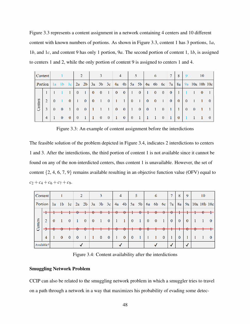
Figure 3.3 represents a content assignment in a network containing 4 centers and 10 different

content with known numbers of portions. As shown in Figure 3.3, content 1 has 3 portions, 1a,

1b, and 1c, and content 9 has only 1 portion, 9a. The second portion of content 1, 1b, is assigned

to centers 1 and 2, while the only portion of content 9 is assigned to centers 1 and 4.

Figure 3.3: An example of content assignment before the interdictions

The feasible solution of the problem depicted in Figure 3.4, indicates 2 interdictions to centers

1 and 3. After the interdictions, the third portion of content 1 is not available since it cannot be

found on any of the non-interdicted centers, thus content 1 is unavailable. However, the set of

content {2, 4, 6, 7, 9} remains available resulting in an objective function value (OFV) equal to

c2 + c4 + c6 + c7 + c9.

Figure 3.4: Content availability after the interdictions

Smuggling Network Problem

CCIP can also be related to the smuggling network problem in which a smuggler tries to travel

on a path through a network in a way that maximizes his probability of evading some detec-

48

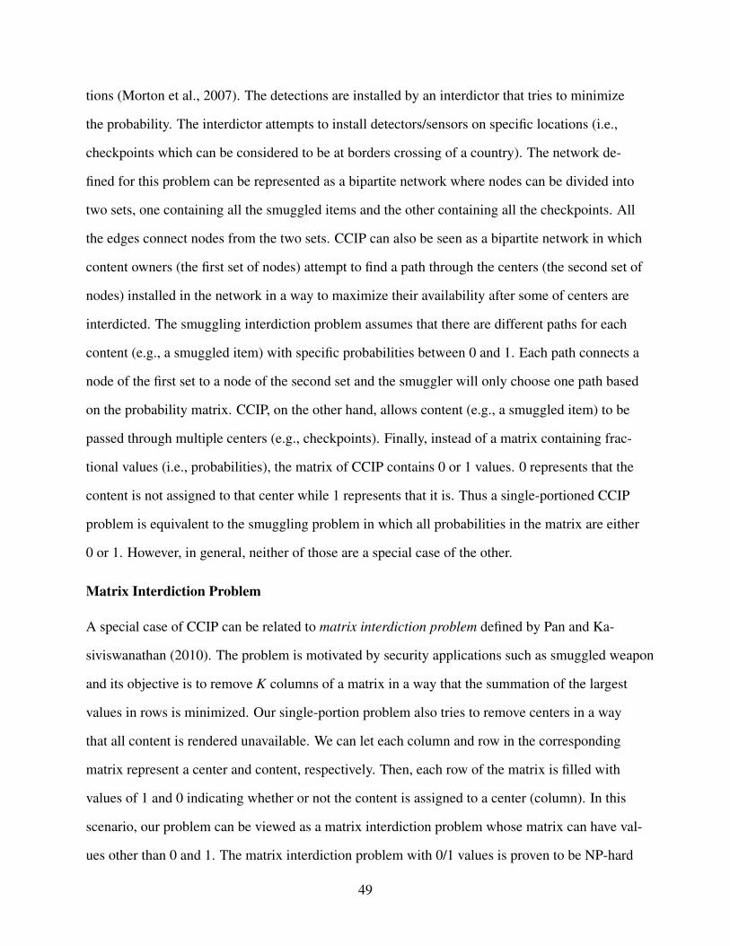
tions (Morton et al., 2007). The detections are installed by an interdictor that tries to minimize

the probability. The interdictor attempts to install detectors/sensors on specific locations (i.e.,

checkpoints which can be considered to be at borders crossing of a country). The network de-

fined for this problem can be represented as a bipartite network where nodes can be divided into

two sets, one containing all the smuggled items and the other containing all the checkpoints. All

the edges connect nodes from the two sets. CCIP can also be seen as a bipartite network in which

content owners (the first set of nodes) attempt to find a path through the centers (the second set of

nodes) installed in the network in a way to maximize their availability after some of centers are

interdicted. The smuggling interdiction problem assumes that there are different paths for each

content (e.g., a smuggled item) with specific probabilities between 0 and 1. Each path connects a

node of the first set to a node of the second set and the smuggler will only choose one path based

on the probability matrix. CCIP, on the other hand, allows content (e.g., a smuggled item) to be

passed through multiple centers (e.g., checkpoints). Finally, instead of a matrix containing frac-

tional values (i.e., probabilities), the matrix of CCIP contains 0 or 1 values. 0 represents that the

content is not assigned to that center while 1 represents that it is. Thus a single-portioned CCIP

problem is equivalent to the smuggling problem in which all probabilities in the matrix are either

0 or 1. However, in general, neither of those are a special case of the other.

Matrix Interdiction Problem

A special case of CCIP can be related to matrix interdiction problem defined by Pan and Ka-

siviswanathan (2010). The problem is motivated by security applications such as smuggled weapon

and its objective is to remove K columns of a matrix in a way that the summation of the largest

values in rows is minimized. Our single-portion problem also tries to remove centers in a way

that all content is rendered unavailable. We can let each column and row in the corresponding

matrix represent a center and content, respectively. Then, each row of the matrix is filled with

values of 1 and 0 indicating whether or not the content is assigned to a center (column). In this

scenario, our problem can be viewed as a matrix interdiction problem whose matrix can have val-

ues other than 0 and 1. The matrix interdiction problem with 0/1 values is proven to be NP-hard

49

(Pan and Kasiviswanathan, 2010). Since a single-portioned CCIP is equivalent to matrix interdic-

tion problem, it can be concluded that CCIP is also an NP-hard problem. .

3.3 Proposed Enhancements to P

To improve the solving time and lower bound to P, we introduce multiple enhancements that are

aimed to better enabling us to solve larger instances. Multiple combinations of these enhance-

ments are to be discussed in Section 3.6. In the following sections, each of the enhancement is

described.

3.3.1 Tightening Constraints

We introduce multiple constraints to reduce the size of feasible region. Three of them showing

improvements when individually added to P are selected for the final enhanced models. In the

following sections, each of them are described.

3.3.1.1 Content Availability Constraint

Let I j be the minimum number of centers to which a portion of content j is assigned (i.e., the

minimum number of interdictions required to make content j unavailable) and I ji a parameter

representing whether (I ji = 1) or not (I ji = 0) any portion of content j is assigned to center i.

These two parameters can be calculated as follows:

I j = mink=1,...,n j

∑i∈I

xijk ∀ j ∈ J (3.7)

I ji = 1 if ∑k=1,...,n j

xijk ≥ 1, 0, otherwise ∀ j ∈ J, ∀i ∈ I (3.8)

Constraint (3.9) requires the content to be available if all of its portions are assigned to more

than B centers since none of the portions can be unavailable after attacking B centers. Constraint

(3.10), on the other hand, forces I j centers from all the centers containing content j to be inter-

50

dicted when content j can be unavailable (i.e., y j0 = 0).

y j0 = 1 ∀ j ∈ J, I j > B (3.9)

∑i∈I, I ji=1

zi− I j ∗ (1− y j0)≥ 0 ∀ j ∈ J, I j ≤ B (3.10)

3.3.1.2 Portion Availability Constraint

Constraint (3.11) forces each y jk to be equal to 0 if the portion is assigned to more than B centers.

This means no matter which centers are interdicted, the portion is still available after the interdic-

tions.

y jk = 0 ∀ j ∈ J,∀k = 1, ...,n j, I j > B (3.11)

3.3.1.3 Symmetry Removing Constraint

As described in constraint (3.3), only one portion must be unavailable in order to make the con-

tent unavailable. In cases where there are multiple portions unavailable, there will be multiple

solutions with the same OFV. In order to eliminate symmetrical solutions, we propose the follow-

ing constraint:

ykj ≤∑

i∈Ixi

jk′(1− xijk)(1− zi), ∀ j ∈ J, k ∈ {2, . . . ,n j}, k′ ∈ {1, . . . ,k−1}. (3.12)

Constraint 3.5 will ensure that the portion (k) whose value of y jk is equal to 1 in constraint (3.3)

is the first unavailable portion. For all those available portions before portion k, we know that y

is equal to 0, thus this constraint impose no restrictions (the right hand side of the inequality will

be a non-zero integer value). We also know that this constraint does not impose any restrictions

on the first unavailable portion (e.g., k1), since on the right hand side of the inequality there is

always an available center for which a portion k′, k′ < k1 is available and we know that xijk1 for

those centers are 0 (since portion k is unavailable). The main purpose of this constraint occurs

51

for the portions after the first unavailable portion. If a portion k, k > k1 is not the first unavailable

portion, this constraint will be y jk ≤ 0 because of the restriction imposed by the first unavailable

portion (i.e., k1) since any time zi is 0, xijk1 is 0.

3.3.2 Modified Objective Function

The inclusion of constraint (3.12) results in a much larger problem. Therefore, we consider a sec-

ond approach to remove the symmetry in the problem. However, we test both of these methods in

Section 3.6

Consider the two models of P1 and P2 with the same feasible region as model P. Model P1

is exactly the same as model P while model P2 has one difference in the OF as shown below. We

denote the difference in the OFs, α, which is equal to (∑ j∈J ∑n jk=1

ky jkn j+1)/|J|.

Model P1

min ∑j∈J

c jy j0 (3.13)

Model P2

min ∑j∈J

c jy j0 +∑ j∈J ∑

n jk=1

ky jkn j+1

|J|(3.14)

Theorem 1 If there exists an optimal solution (OS) to P2, the solution is also optimal to P1 and

the optimal OFV of P1 is the floor of the optimal OFV of P2.

Proof. Let s∗ = (z∗,y∗) be the OS of P2 with OFVP2(s∗). It is also a feasible solution to P1 since

both problems have the same feasible region. Assume s∗ is not optimal for P1 and there exists a

feasible solution s′ which has a better OFV for P1 than s∗ does. Without of loss of generality all

the c j are assumed to be integer valued, therefore, the minimum positive difference between each

52

pair of c j is greater than or equal to 1. So:

OFVP1(s′)≤ OFVP1(s

∗)−1 (3.15)

We also know that s′ is feasible to P2 with an OFVP2(s′) = OFVP1(s

′)+αs′ where αs′ =

(∑ j∈J ∑n jk=1

ky′jkn j+1)/|J| for s′ solution. Since constraint (3.3) indicates at most one of the y jk vari-

ables in this summation is equal to one, we have that ∑n jk=1 ky jk/(n j + 1) < 1, hence it is con-

cluded that 0≤ αs′ < 1. Now we have:

OFVP2(s′) = OFVP1(s

′)+αs′ ≤ OFVP1(s∗)−1+αs′ <

OFVP1(s∗)≤ OFVP1(s

∗)+αs∗ = OFVP2(s∗) (3.16)

This means s′ is a better solution than s∗ for P2 (i.e., OFVP2(s′) < OFVP2(s

∗)), which contradicts

the optimality of s∗ for P2. �

The theorem proves that if the α part of the objective function in P2 is added to the OF of

model P it will not affect the optimal OFV and the floor of the OS’s OFVP2 is the same as OFVP1 .

This part in the OF lets the model to choose the first unavailable portion, which has the smallest

k, for each content to have the value of 1 for its y jk variable. Therefore, based on the fact that the

problem is a minimization one, all the other solutions in which a yk′ j = 1 where k′ is not the first

unavailable portion will not be considered.

3.3.3 Relaxing Problem P

It can be proven that if all y jk variables are binary and the interdiction decision variables are re-

laxed (i.e., zi ∈ [0,1]), then a solution in which all variables are binary still exists. The proof

is available in Appendix 3.A. Since the number of z-variables is smaller than the number of y-

variables, we propose a theorem in which it shows that if z-variables are binary, then all the y-

variables can be relaxed without changing the problem’s OFV.

53

Theorem 2 If all y jk variables are relaxed in problem P (i.e., y jk ∈ [0,1]), it will not change the

optimal OFV. Also all y j0 will be binary valued in the optimal solution and the solution can be

modified so that all other y variable are also binary valued. The modified solution is also an opti-

mal solution to problem P.

Proof. Let problem P3 be the same as problem P but with relaxed y-variables. Assume s∗ =

(z∗,y∗) is an OS of problem P3 and it contains some fractional y-values. Note that the OFs of

both problems are the same and problem P3’s feasible region contains problem P’s feasible re-

gion. If we find a solution for problem P which has the optimal OFV of problem P3, we know it

is an OS of problem P.

Since the interdiction of each content is purely dependent on the values of zi variables and

independent of other content and also in the modification, we only change the y-variables (and

not the z), without loss of generality we can assume that we only have one content in our prob-

lem. There can be 4 cases defined for y values in s∗ as follows:

1- All y∗jk, ∀k ≥ 0 are binary valued

2- y∗j0 is binary valued and at least one of the y∗jk, ∀k ≥ 1 has a fractional value

3- y∗j0 has a fractional value and all the other y∗jk, ∀k ≥ 1 are either 0 or 1

4- y∗j0 and at least one of y∗jk, ∀k ≥ 1 have fractional values

Case 1: If all the y∗jk variables are binary valued for content j, then there is nothing required to be

done to modify the solution and it is an OS to problem P.

Case 2: Having a binary value for y∗j0 means the the solution can be modified to a solution which

is also feasible to problem P. Since there are some fractional values for y∗jk, ∀k ≥ 1, based on

constraint (3.3) it can be concluded that y∗j0 cannot be 1, hence it is 0. Constraint (3.2) is the only

constraint that includes y-variables for portions. Depending on the binary values of z∗i variables,

constraint (3.2) can be equal to: y∗jk ≤ 0 or y∗jk ≤ 1, ∀k ≥ 1. If there is at least one k′ for which

y∗jk′ has a fractional value, it means for none of the centers, constraint (3.2) became y∗jk′ ≤ 0 and

that is why y∗jk′ can have a fractional value. If so, all the other possible fractional values of y∗jk,

54

∀k = 1, ..., n j, k 6= k′ can be reduced to 0, so that y∗jk′ can become 1. Constraint (3.3) will remain

satisfied and since y∗j0 has still the same value, 0, the OFV will not change. This means the mod-

ified solution is also feasible to problem P (it is still satisfying other constraint since they do not

include y∗jk, ∀k ≥ 1) and has the same OFV as s∗.

Case 3: This case cannot occur because of constraint (3.3).

Case 4: If there is at least one portion k′ with fractional value, for all centers i containing this

portion, constraint (3.2) under fixed z∗ reduces to y∗jk′ ≤ 1. This means by increasing the value of

y∗jk′ to 1 and setting all the other y∗jk, ∀k = 1, ..., n j, k 6= k′ to 0 (whether they are already 0 or they

have fractional values), y∗j0 can be equal to 0. This means the OFV can be reduced by the product

of c j and the previous fractional value of y∗j0 which contradicts with the optimality of the solution

s∗. So this case cannot occur. �

Note that in a case with multiple content, the modification can occur for each one of them

independently. So any OS of P3 can be modified to a solution that is also feasible and optimal to

problem P. We also know that all the values of y∗j0 are binary in the OS of P3 and we just need to

modify the values of y for portions.

3.3.4 Custom Branching

Theorem 2 showed that y variables can be relaxed if all the z variables are forced to be binary val-

ued. Also, in the GA (Section 3.4) each solution is just represented by a chromosome containing

z values and then y values can be calculated based on them. These motivated us to generate a cus-

tom variable selection rule to control branching in the CPLEX branch-and-bound solver. Three of

the considered branching rules will be explained in the following two sections.

3.3.4.1 Branching on z-variables

In this custom branching, at each fractional-valued node, z variables’ values will be checked ac-

cording to the order described in the next paragraph. Then, the first z variable (e.g., zi) with frac-

tional value will be selected to be branched. Therefore, one of the two nodes derived from the

55

current node on the branch will have zi = 1 as a new constraint and the other will have zi = 0.

In a preprocessing step prior to beginning the solution algorithm, all centers will be sorted

based on the “worth” of all content portions assigned to them. The worth of each center can be

calculated based on the total value of content portions assigned to it. If it is a single-portioned

problem, the worth of center j is equal to the summation of c j-values of all content assigned to

it (i.e., ∑ j∈J ∑n jk=1 x jkc j). If it is a multiple-portioned problem, depending on the number of con-

tent j’s portions assigned to a center, only a fraction of c j will be considered in this value (i.e.,

∑ j∈J ∑n jk=1(x jk/n j)c j). For example if content j has 3 portions and value of c j and center i con-

tains two of them, worth of center i will be contain the value of 23c j. After each center’s worth is

calculated, they will be sorted in an decreasing order. For instance, in Figure 3.1 the 3 values for

centers 1, 2, and 3 are calculated as follows:

center 1: (2/2)c1 +(2/3)c2 +(3/4)c3 = 50+40+75 = 165

center 2: (1/2)c1 +(1/3)c2 +(1/4)c3 = 25+20+25 = 70

center 3: (1/2)c1 +(1/3)c2 +(2/4)c3 = 25+20+50 = 95

Therefore, the decreasing order of centers is: center 1 - center 3 - center 2. This order will be

used in Sections 3.3.4 and 3.4.

56

Figure 3.1: An example for preprocessing

3.3.4.2 Branching on yj0-variables

Testing the first custom branching motivated us to do the same for y variables. Since an important

y variable is y j0, we attempt to force branching on y j0 according to an order. Each y j0 will be

assigned a value, called w j. Each w j parameter indicates worth of the associated y j0 variable and

is determined by (3.17). A w j is more if its c j value is higher and it is assigned to less number of

centers which makes it easier to be unavailable.

w j =c j

∑i∈I

xijk

∀ j ∈ J (3.17)

However, the worth of each content is better to be dynamically calculated during the branch and

bound procedure when values (including fractional values) of z variables are known for each

node. Then, the w parameters are calculated by (3.18).

w j =c j

∑i∈I, zi=0

xijk

∀ j ∈ J (3.18)

57

(3.18) differs from the order in (3.17) since it considers how hard it is for the content to be un-

available now that some of the zi variables are known (i.e., interdiction decisions for the associ-

ated centers are made). Then, the same procedure as Section 3.3.4.1 is performed when branch-

ing only occurs on y j0 variables according to the order described in (3.18).

3.3.4.3 Branching on z-variables and yj0-variables

We also consider a mixed branching. In this branching, an initial parameter is determined at the

beginning of solving IP. Then, for each node a discrete Uniform variable between [1,100] is

generated. If the value of the generated variable is less than the parameter, then the next branch

is performed on the first z variable according to order described in 3.3.4.1 that has a fractional

value; otherwise it is performed on the first y j0 according to order (3.18) with a fractional value.

Note that if the parameter is 0, the branching is equal to the one explained in Section 3.3.4.2

and if it is equal to 100, the branching discussed in Section 3.3.4.1 is performed.

3.4 Genetic Algorithm (GA)

Since solving time of the IP model for large sized problems is high, we developed a GA whose

solution in a short amount of time can assist IP as an initial solution to reduce its solving time.

The steps of the proposed GA are described as follows:

Step 1. An initial population is randomly generated.

Step 2. The fitness of each individual is computed.

Step 3. At each generation the first two individuals are the two elites, taken from the last

generation, and the remaining population size - 2 individuals are selected using a tourna-

ment of size of two.

Step 4. If possible, a crossover is then applied on each pair of parents, except for the first

two.

Step 5. Two rounds of mutations with fixed probabilities are applied on offspring, except

for the first two offspring.

58

Step 6. If none of the termination criteria is met, return to step 3.

In the following sections, each of the steps will be explained.

3.4.1 Encoding a Chromosome

Given the results from Theorem 2, we define each chromosome only based on the z-variables.

Each chromosome, representing a solution, has one part containing |I| (number of centers) genes.

A gene is equal to 1, if the corresponding center is interdicted and 0, if it is not interdicted.

In Figure 3.4.1, a chromosome representation of one feasible solution is presented. This

chromosome represents a problem in which there are 7 centers and 3 (2, 3, and 7) of them are

assumed to be interdicted in the inner problem.

Figure 3.1: Representation of a chromosome

3.4.2 Initial Population

The fist chromosome in the first population is based on order calculated in preprocessing part.

The first B centers according to the order will be equal to 1 and the rest of the genes will be equal

to 0. This follows the same greedy algorithm developed in Pan and Kasiviswanathan (2010). To

generate the rest of the population, for each chromosome B centers are randomly chosen to be

interdicted and their genes become 1, then the rest of the genes will be equal to 0. This occurs

until population size, PS, chromosomes are generated. Multiple PSes were tested with different

combination of other parameters. PS=50 showed to be the most effectiveness for all sizes (small

to large). Larger PSs (e.g.,100) cause each generation to take more time for larger instances and

eventually affected the best fitness. On the other hand, smaller PSes (e.g., 20), made improve-

ment between iterations slower and were not as effective as PS=50.

59

3.4.3 Fitness Calculation

To calculate the fitness of each chromosome, each content’s portion gets checked to see that it is

available on at least one of the centers which are not interdicted. If there is at least one portion

which is not available on any of the unattached centers, it means the content is unavailable and

this will not affect the fitness value. If, however, a content is available, its c j will be added to the

fitness value. The first population of chromosomes will be the children who will generate the first

set of parents at iteration 1.

3.4.4 Selection

At each iteration the first two parents of each population will be the two elites of the last popu-

lation. Other parents are selected using a tournament of size of two which means two random

parents will be chosen among all the parents and the one with lower fitness will be selected as the

next parent until we have PS parents. Note that at each iteration the best child will be replaced by

the global best chromosome if its fitness is less than the global best chromosome’s fitness.

3.4.5 Crossover

At each iteration, one single point crossover is used to generate offspring for all pairs of parents

except for the first two. The one point crossover may occur at a point before which both parents

have the same number of genes equal to 1, so that both of the children after the crossover still

have B numbers of genes equal to 1.

Starting from the 3rd parent, a crossover occurs for each pair of parents. In order to do

a crossover on the parents, a crossover point needs to be designated. The initial value for this

point is b|I|/2c. To determine if the crossover can occur for this point, the total number of genes

equaled to one from the first gene up to the candidate point are counted. If the numbers are equal

for both parents, then a crossover is performed; otherwise, in an iterative process, points before

and after the initial point will be considered respectively. For example, if the two parents have

60

|I| = 20 genes, point 10 is initially the candidate of the crossover. If the crossover cannot be per-

formed, then point 9 (and then 11) are the candidate. The numbers that will be considered will

be in this order: 10, 9 , 11, 8, 12, 7, 13, 6, 14, etc. The search stops if it reaches to a point for

which the crossover can be performed or it reaches to the first or the last center since even if the

crossover is performed, no difference will result between the children and the parents.

For example, in Figure 3.2, the first candidate point for the crossover is 4. The first parent

has 2 genes equal to 1 (genes 2 and 3) before the point while the second parent has only one gene

equal to 1 (gene 1). Therefore, the crossover cannot occur at point 4. The next point to be consid-

ered is point 3. There are two genes of parent 1 equal to 1 and 1 gene of parent 2, so point 5 will

be considered next. Still the numbers of ones before the point 5 are not equal. The next point to

be considered is point 2 before which both parents have the same numbers of genes equal to 1.

Therefore, the crossover occur at point 2.

61

Figure 3.2: Selection of a point for a crossover

As shown in Figure 3.3, child 1 inherits the first two genes of parent 2 and the others from parent

1 and child 2 inherits the first two genes from parent 1 and the others from parent 2.

62

Figure 3.3: Representation of the crossover

In general, for each crossover, this process continues between points on the left side and then

right side consecutively until the first or the last centers. Note that our search does not start from

the first gene because the goal of our crossover is that both offspring inherit the most from both

parents. Thus, it is desirable for the crossover to happen at a point closer to the middle gene.

However, based on the chromosome structure, the crossover cannot occur for all pairs of par-

ents. The lower the number of the centers, the smaller chance there is to find a point at which the

crossover can happen. Also, by increasing the number of centers, the chance of finding such point

will be high and as a result the crossover will occur for almost all the pairs of parents. Therefore,

a maximum rate of crossover is enforced to prevent a crossover from occurring between all pairs.

After testing multiple values, 60% was chosen since it showed the most rapid improvement for

various problem sizes.

3.4.6 Mutation

After generating PS children, two consecutive rounds of single point mutations are applied on

each child by probabilities of 0.25. This means there is a 0.0625 (0.26*0.25) chance that a child

has two single point mutations. The probability of the first mutation is equal to 0.5 for prob-

lems with 5000 content or more, but the second mutation’s probability remains 0.25. In order

to do a mutation, two different genes with different values will be chosen and their values will be

63

swapped. As shown in Figure 3.4, gene 3 and 4 switch their values after mutation.

Figure 3.4: Mutation Representation

After the mutation, all children’s fitnesses will be calculated and the best of them will replace the

global best solution if it has a lower fitness. All children will be then considered as candidates to

be parents for the next iteration.

3.4.7 Stopping Criteria

This process continues until one of the stopping criteria according to 3.1 is met. For instances

with 4000 content they are: 1- 1000 total iterations, 2- 100 iterations without improvement in the

best chromosome’s fitness, 3- 120 seconds time limit. These values have been fixed after multiple

runs of tests to make sure there is enough time for improvement while not spend extra time when

the chance of getting better solution is low.

Table 3.1: GA’s stopping criteria

# of time maximum maximum iterationscontent limit (sec) iterations without improvement

1-99 30 1000 25100-999 60 1000 50

1000-4999 120 1000 1005000-9999 300 1000 300

10000-19999 600 1000 40020000+ 1200 1000 500

64

3.5 Other Attempted Methods

Given that the problem is NP-hard, different exact large-scale solution methods have been tested.

In the following paragraphs the ones which did not outperform the original model will be briefly

described.

Reformulation-Linearization Technique (RLT): Two sets of first level RLT (Sherali and Adams,

1998) were tested on multiple instances (single and multiple portioned content) to see if it can

reduce the solving time of the problem or generate a good lower bound for the P formulation

in a shorter amount of time. Although it managed to reach to the optimal solution for most of

the single portioned instances, the efforts did not last due to the number of variables and con-

straints added to the formulation which caused memory loss. Also, solving time in almost all the

instances were not comparable with P’s.

Benders Decomposition: Given that z variables can be relaxed, we attempted to solve the prob-

lem with a Benders decomposition (BD) approach. BD requires its subproblem (SP) to be a con-

tinuous linear or nonlinear programming problem, so that the dual of the SP can be used to obtain

optimality and feasibly cuts. All the variables and constraints containing the relaxed z variables

were moved to the subproblem. Since coefficients of all z variables in the original problem’s OF

is 0, only feasibility cuts were applied to the master problem (MP) after each iteration. Two BD

approaches were implemented, the traditional iterative BD and BD with application of Lazy Con-

straint Callback which was described in section ??. Unfortunately, none of the approaches could

outperform the P even for small instances.

Logic-based Decomposition: We also pursued a logic-based decomposition approach which

is inspired by Benders decomposition approach. Same approach with application of Lazy Con-

straint Callback, as described in Chapter 2 and shown in Figure 2.5, was applied for this problem.

The difference with the BD described in the previous paragraph was that instead of solving the

dual of the SP, the original SP was solved and a newly defined feasibility cut, which was respon-

sible to cut the current node was applied. Again, the solving time could not outperform the P

65

solving time.

3.6 Computational Results

100 different instances with 10 to 30000 content and 3 to 300 centers were generated. The data of

different instances are presented in Table 3.1. There are two types of problems, single portioned

(S) and multiple-portioned (M). In all the M instances, the number of portions is randomly cho-

sen to be between 3 to 7. There are 50 single portioned problems (S1-S50) and 50 multiple ones

(M1-M50). c js are randomly generated between 10 to 40.

Table 3.1: Single and multiple portioned instances data

Single Multiple # of # of # of Single Multiple # of # of # ofinstance # instance # content servers interdictions instance # instance # content servers interdictions

S1 M1 10 3 1 S26 M26 4000 50 45S2 M2 10 3 2 S27 M27 7000 70 5S3 M3 20 4 1 S28 M28 7000 70 10S4 M4 20 4 3 S29 M29 7000 70 35S5 M5 50 6 2 S30 M30 7000 70 60S6 M6 50 6 4 S31 M31 10000 100 5S7 M7 100 10 2 S32 M32 10000 100 10S8 M8 100 10 7 S33 M33 10000 100 20S9 M9 200 15 3 S34 M34 10000 100 50

S10 M10 200 15 7 S35 M35 10000 100 90S11 M11 200 15 12 S36 M36 15000 150 10S12 M12 400 20 4 S37 M37 15000 150 20S13 M13 400 20 10 S38 M38 15000 150 30S14 M14 400 20 16 S39 M39 15000 150 75S15 M15 800 25 5 S40 M40 15000 150 120S16 M16 800 25 12 S41 M41 20000 200 10S17 M17 800 25 22 S42 M42 20000 200 20S18 M18 1000 30 5 S43 M43 20000 200 40S19 M19 1000 30 15 S44 M44 20000 200 100S20 M20 1000 30 25 S45 M45 20000 200 150S21 M21 2000 40 5 S46 M46 30000 300 15S22 M22 2000 40 20 S47 M47 30000 300 30S23 M23 2000 40 35 S48 M48 30000 300 60S24 M24 4000 50 5 S49 M49 30000 300 150S25 M25 4000 50 25 S50 M50 30000 300 250

As shown in Table 3.1, each content number has multiple instances with different values of B

(e.g., problems S1 and S2). Note that the problems with the same letter (S or M) and number of

content have same assignments such as problems S3 and S4 whose only difference is the number

of B. All instances were solved by CPLEX 12.6.3 on a 12-core 12 GB computer. Time limit for

66

each instance is shown in Table 3.2. A stopping gap of 0.001% was used, where

gap =best integer solution’s OFV − best linear programming relaxation solution’s OFV

best integer solution’s OFV∗100

Table 3.2: Time limit

Problem # Time limit (min)

S1-S30 30S31-S40 60S41-S50 120

M1-M30 60M31-M40 120M41-M50 180

Each enhancement described in Section 3.3 was individually run on a subset of the S and M in-

stances. Then, combinations show to improve either on solving time, objective function value,

or lower bound (LB) in the assigned time limit were pursued. Figure 3.1 presents the implemen-

tation that incorporates multiple enhancements. Initially, the preprocessing occurs which sort

centers based on the order described in Section 3.3.4.1. Then, the GA is run and its best solution

is used as an initial solution to an enhanced version of P which exploits a custom branching. Both

solving time or gap will be our base of comparison between P solved with default CPLEX and

the enhanced version of P that also makes use of the proposed genetic algorithm.

67

Figure 3.1: An illustration of using multiple enhancements in a model

3.6.1 Different IP Formulations for Solving Single-Portioned (S) Instances

After attempting multiple combinations of the implementation features, the three best were con-

sidered in a full comparison with P solved by a standard IP solver. The implementations consid-

ered are defined as follows:

– P, which is the original IP

– PS1 , in which y variables are binary. It includes constraints (3.9), (3.10), and (3.11), and

utilizes GA and branching on z variables as discussed in Section (3.3.4.1).

– PS2 , in which y variables are continuous. It includes constraints (3.9), (3.10), and (3.11), and

utilizes GA and branching on z variables as discussed in Section (3.3.4.1).

– PS3 , in which y variables are binary. It includes constraints (3.9), (3.10), and (3.11), and

utilizes GA and branching on z and y j0 variables as discussed in Section (3.3.4.3) with theparameter of 50.

68

Table 3.3 contains all the data regarding the enhancements used in the 4 IP models used to solve

S instances.

Table 3.3: Implementations to solve S problems

IP Binary y Continuous y GA Constraint Constraint Constraint Branch Branch onmodel variables variables (3.9) (3.10) (3.11) on z y and z

P X

PS1 X X X X X X

PS2 X X X X X X

PS3 X X X X X X

3.6.2 Different IP Formulations for Solving Multiple-Portioned (M) Instances

Five different models (including the original P) are represented in this section to solve M prob-

lems. All models contain binary valued y variables as the continuous y variables were not as ef-

ficient for M problems. Note that the utilization of constraint (3.12) or the modified OF in (3.14)

are only performed when we have an M instance.

– P, which is the original P

– PM1 , which includes constraints (3.9), (3.10), (3.11), and (3.12) and utilizes GA .

– PM2 , which includes constraints (3.9), (3.10), and (3.11), and (3.12), and utilizes GA and

branching on z variables as discussed in Section (3.3.4.1).

– PM3 , which includes constraints (3.9), (3.10), and (3.11) and OF in (3.14), and utilizes GA

and branching on z variables as discussed in Section (3.3.4.1).

– PM4 , which includes constraints (3.9), (3.10), and (3.11), and (3.12), and utilizes GA and

branching on z and y j0 variables as discussed in Section (3.3.4.3) with the parameter of 50.

Table 3.4 contains information regarding enhancements included in the 5 models used to solve M

instances.

69

Table 3.4: Implementations to solve M problems

GA Constraint Constraint Constraint Constraint OF Branch Branch onModels (3.9) (3.10) (3.11) (3.12) (3.14) on z y and z

P

PM1 X X X X X

PM2 X X X X X X

PM3 X X X X X X

PM4 X X X X X X

Note that only z values taken from the best solution of the GA are fed to the models as an ini-

tial solution. We also tested different CPLEX parameters and our findings suggest the following

values settings: Effort Level =1 (default), Advance=1 (default), Emphasis = 1 (feasibility over

optimality).

3.6.3 Results of Single-Portioned Instances

Out of the 50 S instances, 30 were solved by all the 4 models during the specified time limits. Ta-

ble 3.5 shows the best OFV, LB, solving time and, OFV of the best solution obtained form GA

for each instance. Note that GA took a minimum of 2% and a maximum of 100% of the total the

solving times of each model (without considering the instances whose both solving time and GA

time are 0.0 seconds). Models PS1 , PS

2 , and PS3 spent an average of 40%, 39%, and, 46% of the

total solving time in GA, respectively. Details of GA times can be found in Appendix 3.B. The

stopping criterion which stopped the GA for most of the 50 S instances was the number of itera-

tions without improvement. It stopped 45, 48, and 44 instances for PS1 , PS

2 , and PS3 , respectively.

The remaining instances were stopped by the maximum time limit.

The best solving times are highlighted with blue color in Table 3.5. Problems S1-S11 were

solved in approximately 0.0 seconds, thus all of the 4 models are highlighted. As expected, many

of the smaller instances are solved in shorter amount of time by P. However, PS1 managed to

solve three of the medium sized instances (S22, S25, and S30) quicker than P.

70

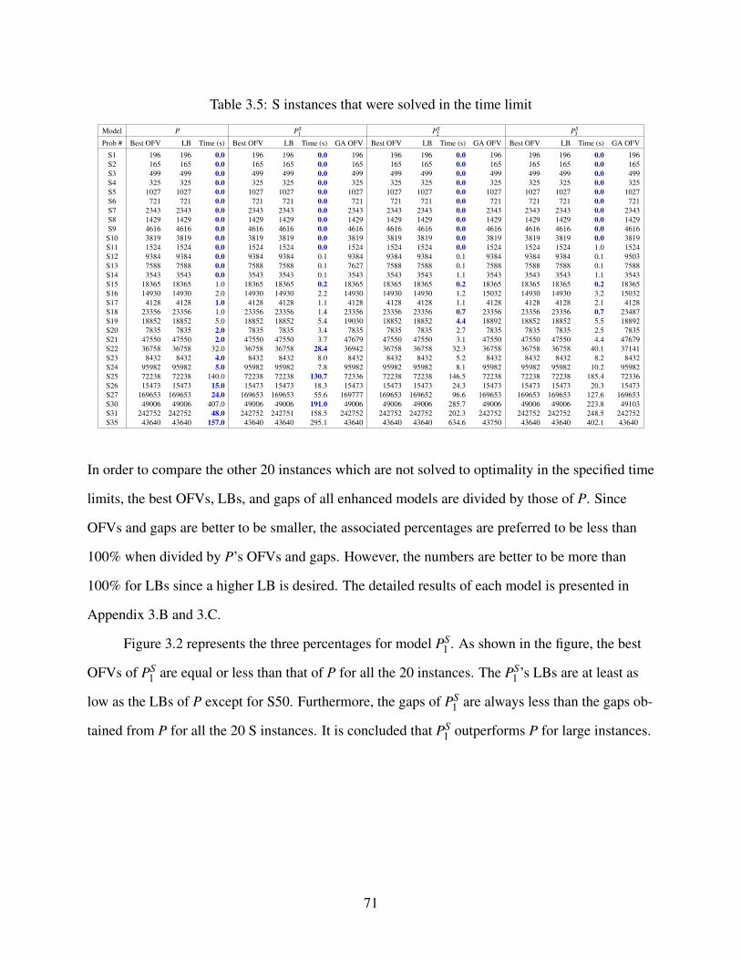
Table 3.5: S instances that were solved in the time limit

Model P PS1 PS

2 PS3

Prob # Best OFV LB Time (s) Best OFV LB Time (s) GA OFV Best OFV LB Time (s) GA OFV Best OFV LB Time (s) GA OFV

S1 196 196 0.0 196 196 0.0 196 196 196 0.0 196 196 196 0.0 196S2 165 165 0.0 165 165 0.0 165 165 165 0.0 165 165 165 0.0 165S3 499 499 0.0 499 499 0.0 499 499 499 0.0 499 499 499 0.0 499S4 325 325 0.0 325 325 0.0 325 325 325 0.0 325 325 325 0.0 325S5 1027 1027 0.0 1027 1027 0.0 1027 1027 1027 0.0 1027 1027 1027 0.0 1027S6 721 721 0.0 721 721 0.0 721 721 721 0.0 721 721 721 0.0 721S7 2343 2343 0.0 2343 2343 0.0 2343 2343 2343 0.0 2343 2343 2343 0.0 2343S8 1429 1429 0.0 1429 1429 0.0 1429 1429 1429 0.0 1429 1429 1429 0.0 1429S9 4616 4616 0.0 4616 4616 0.0 4616 4616 4616 0.0 4616 4616 4616 0.0 4616

S10 3819 3819 0.0 3819 3819 0.0 3819 3819 3819 0.0 3819 3819 3819 0.0 3819S11 1524 1524 0.0 1524 1524 0.0 1524 1524 1524 0.0 1524 1524 1524 1.0 1524S12 9384 9384 0.0 9384 9384 0.1 9384 9384 9384 0.1 9384 9384 9384 0.1 9503S13 7588 7588 0.0 7588 7588 0.1 7627 7588 7588 0.1 7588 7588 7588 0.1 7588S14 3543 3543 0.0 3543 3543 0.1 3543 3543 3543 1.1 3543 3543 3543 1.1 3543S15 18365 18365 1.0 18365 18365 0.2 18365 18365 18365 0.2 18365 18365 18365 0.2 18365S16 14930 14930 2.0 14930 14930 2.2 14930 14930 14930 1.2 15032 14930 14930 3.2 15032S17 4128 4128 1.0 4128 4128 1.1 4128 4128 4128 1.1 4128 4128 4128 2.1 4128S18 23356 23356 1.0 23356 23356 1.4 23356 23356 23356 0.7 23356 23356 23356 0.7 23487S19 18852 18852 5.0 18852 18852 5.4 19030 18852 18852 4.4 18892 18852 18852 5.5 18892S20 7835 7835 2.0 7835 7835 3.4 7835 7835 7835 2.7 7835 7835 7835 2.5 7835S21 47550 47550 2.0 47550 47550 3.7 47679 47550 47550 3.1 47550 47550 47550 4.4 47679S22 36758 36758 32.0 36758 36758 28.4 36942 36758 36758 32.3 36758 36758 36758 40.1 37141S23 8432 8432 4.0 8432 8432 8.0 8432 8432 8432 5.2 8432 8432 8432 8.2 8432S24 95982 95982 5.0 95982 95982 7.8 95982 95982 95982 8.1 95982 95982 95982 10.2 95982S25 72238 72238 140.0 72238 72238 130.7 72336 72238 72238 146.5 72238 72238 72238 185.4 72336S26 15473 15473 15.0 15473 15473 18.3 15473 15473 15473 24.3 15473 15473 15473 20.3 15473S27 169653 169653 24.0 169653 169653 55.6 169777 169653 169652 96.6 169653 169653 169653 127.6 169653S30 49006 49006 407.0 49006 49006 191.0 49006 49006 49006 285.7 49006 49006 49006 223.8 49103S31 242752 242752 48.0 242752 242751 158.5 242752 242752 242752 202.3 242752 242752 242752 248.5 242752S35 43640 43640 157.0 43640 43640 295.1 43640 43640 43640 634.6 43750 43640 43640 402.1 43640

In order to compare the other 20 instances which are not solved to optimality in the specified time

limits, the best OFVs, LBs, and gaps of all enhanced models are divided by those of P. Since

OFVs and gaps are better to be smaller, the associated percentages are preferred to be less than

100% when divided by P’s OFVs and gaps. However, the numbers are better to be more than

100% for LBs since a higher LB is desired. The detailed results of each model is presented in

Appendix 3.B and 3.C.

Figure 3.2 represents the three percentages for model PS1 . As shown in the figure, the best

OFVs of PS1 are equal or less than that of P for all the 20 instances. The PS

1 ’s LBs are at least as

low as the LBs of P except for S50. Furthermore, the gaps of PS1 are always less than the gaps ob-

tained from P for all the 20 S instances. It is concluded that PS1 outperforms P for large instances.

71

Figure 3.2: Comparison of PS1 OFV, LB, and gap to P for S instances which were not solved to

optimality by the majority of the models

Figure 3.3 compares model PS2 to P. PS

2 ’s OFVs are at least as low as the ones obtained from P

and the LBs are higher than P’s in majority of the instances. Except for one problem (S48), gaps

of PS2 are lower than P, however, they are not as low as the PS

1 .

72

Figure 3.3: Comparison of PS2 OFV, LB, and gap to P for S instances which were not solved to

optimality by the majority of the models

Figure 3.4 compares model PS3 to P. The difference between the two models (P and PS

3 ) are no-

ticeable for relatively smaller sized instances as shown in the figure. Higher LBs assist P to reach

to lower gaps compared to PS3 since the best OFVs are the same. For larger instances, it can be

concluded that the best PS3 can perform is to reach the gap of P. Therefore, PS

3 is not comparable

with P, PS1 , and PS

2 .

73

Figure 3.4: Comparison of PS3 OFV, LB, and gap to P for S instances which were not solved to

optimality by the majority of the models

In order to compare the three enhanced models (PS1 , PS

2 , and PS3 ) simultaneously, the relative gaps

(compared to P) are shown in Figure 3.5. As mentioned earlier, PS3 is not comparable with P, thus

the race is between PS1 and PS

2 since they both outperformed P’s gaps. It can be concluded that

between PS1 and PS

2 , PS1 is capable of reaching to better gaps for relatively large instances. Also, it

showed its capability to outperform P for some medium instances (see Table 3.5).

The results show that branching on z variables (in PS1 and PS

2 ) has better performance than

when mixed branching in Section 3.3.4.3 occurs with the parameter of 50 (in PS3 ). Other values

of the parameter were also tested. For example, 0 showed to be not as efficient as 5 which means

branching on y variables are not as helpful as branching on z.

74

Figure 3.5: Gap comparison among PS1 , PS

2 , and PS3 for S instances which were not solved to

optimality by the majority of the models

Table 3.6, contains details of the two problems P and PS1 . Each model’s solving time and gap are

bold if they are better than the other model. Since each gap is calculated based on the best OFV

and LB of its associated model, we also compare the best OFVs and LBs of the models sepa-

rately. As shown in the table, the better OFV and LB for each instance between the two model

are highlighted by blue and violet color, respectively. It can be concluded that model PS1 can out-

perform model P in reaching to lower best OFVs and higher LBs as the problem size increases.

75

Table 3.6: P vs. PS1 for S instances

Model P PS1

Prob # Content # Center # B Best OFV LB Gap (%) Time (s) Best OFV LB Gap (%) Time (s) GA’s best OFV

S1 10 3 1 196 196 0.0% 0.0 196 196 0.0% 0.0 196S2 10 3 2 165 165 0.0% 0.0 165 165 0.0% 0.0 165S3 20 4 1 499 499 0.0% 0.0 499 499 0.0% 0.0 499S4 20 4 3 325 325 0.0% 0.0 325 325 0.0% 0.0 325S5 50 6 2 1027 1027 0.0% 0.0 1027 1027 0.0% 0.0 1027S6 50 6 4 721 721 0.0% 0.0 721 721 0.0% 0.0 721S7 100 10 2 2343 2343 0.0% 0.0 2343 2343 0.0% 0.0 2343S8 100 10 7 1429 1429 0.0% 0.0 1429 1429 0.0% 0.0 1429S9 200 15 3 4616 4616 0.0% 0.0 4616 4616 0.0% 0.0 4616

S10 200 15 7 3819 3819 0.0% 0.0 3819 3819 0.0% 0.0 3819S11 200 15 12 1524 1524 0.0% 0.0 1524 1524 0.0% 0.0 1524S12 400 20 4 9384 9384 0.0% 0.0 9384 9384 0.0% 0.1 9384S13 400 20 10 7588 7588 0.0% 0.0 7588 7588 0.0% 0.1 7627S14 400 20 16 3543 3543 0.0% 0.0 3543 3543 0.0% 0.1 3543S15 800 25 5 18365 18365 0.0% 1.0 18365 18365 0.0% 0.2 18365S16 800 25 12 14930 14930 0.0% 2.0 14930 14930 0.0% 2.2 14930S17 800 25 22 4128 4128 0.0% 1.0 4128 4128 0.0% 1.1 4128S18 1000 30 5 23356 23356 0.0% 1.0 23356 23356 0.0% 1.4 23356S19 1000 30 15 18852 18852 0.0% 5.0 18852 18852 0.0% 5.4 19030S20 1000 30 25 7835 7835 0.0% 2.0 7835 7835 0.0% 3.4 7835S21 2000 40 5 47550 47550 0.0% 2.0 47550 47550 0.0% 3.7 47679S22 2000 40 20 36758 36758 0.0% 32.0 36758 36758 0.0% 28.4 36942S23 2000 40 35 8432 8432 0.0% 4.0 8432 8432 0.0% 8.0 8432S24 4000 50 5 95982 95982 0.0% 5.0 95982 95982 0.0% 7.8 95982S25 4000 50 25 72238 72238 0.0% 140.0 72238 72238 0.0% 130.7 72336S26 4000 50 45 15473 15473 0.0% 15.0 15473 15473 0.0% 18.3 15473S27 7000 70 5 169653 169653 0.0% 24.0 169653 169653 0.0% 55.6 169777S28 7000 70 10 167593 164391 1.9% 1809.0 167641 165101 1.5% 1807.3 167692S29 7000 70 35 139789 114102 18.4% 1807.0 139668 119166 14.7% 1809.0 139668S30 7000 70 60 49006 49006 0.0% 407.0 49006 49006 0.0% 191.0 49006S31 10000 100 5 242752 242752 0.0% 48.0 242752 242751 0.0% 158.5 242752S32 10000 100 10 241032 236680 1.8% 3614.0 241026 238533 1.0% 3610.5 241026S33 10000 100 20 236006 216798 8.1% 3624.0 235620 220794 6.3% 3614.2 235620S34 10000 100 50 195746 150719 23.0% 3605.0 194604 161435 17.0% 3608.0 194604S35 10000 100 90 43640 43640 0.0% 157.0 43640 43640 0.0% 295.1 43640S36 15000 150 10 365623 358772 1.9% 3615.0 365527 360439 1.4% 3614.1 365527S37 15000 150 20 363480 326994 10.0% 3613.0 362895 338181 6.8% 3613.1 362895S38 15000 150 30 359894 305602 15.1% 3600.0 359479 319494 11.1% 3610.9 359479S39 15000 150 75 334107 196076 41.3% 3600.0 316156 219033 30.7% 3610.8 316156S40 15000 150 120 174818 80593.2 53.9% 3600.0 163321 106860 34.6% 3607.0 163321S41 20000 200 10 488665 481376 1.5% 7218.0 488646 483349 1.1% 7221.4 488647S42 20000 200 20 487635 450543 7.6% 7200.0 487668 459296 5.8% 7214.1 487668S43 20000 200 40 484903 405859 16.3% 7206.0 484263 417346 13.8% 7211.5 484321S44 20000 200 100 464586 252321 45.7% 7218.0 445402 278758 37.4% 7217.0 445402S45 20000 200 150 330251 128777 61.0% 7200.0 309045 150119 51.4% 7213.5 309045S46 30000 300 15 735313 710255 3.4% 7200.0 735330 714713 2.8% 7210.4 735333S47 30000 300 30 734751 669130 8.9% 7200.0 734672 675123 8.1% 7219.1 734727S48 30000 300 60 733547 596774 18.6% 7200.0 733272 598818 18.3% 7213.5 733349S49 30000 300 150 717367 374263 47.8% 7200.0 700341 374244 46.6% 7208.3 700341S50 30000 300 250 480218 126042 73.8% 7214.0 450350 124763 72.3% 7207.3 450350

3.6.4 Results of Multiple-Portioned Instances

Out of the 50 M instances, 25 were solved by all the 4 models during the specified time limits.

OFV, LB, solving time and, OFV of the best solution obtained form GA for each of the instances

76

are presented in Table 3.7. The GA took a minimum of 0% and a maximum of 100% of the total

the solving times of each model. Models PM1 , PM

2 , PM3 , and PS

4 spent an average of 23%, 27%,

29%, and, 23% of the total solving time in the GA, respectively. The number of iterations without

improvement criterion stopped the GA for 34, 34, 33, and, 33 instances for PM1 , PM

2 , PM3 , and PM

4

models, respectively. The remaining instances were stopped by the maximum time limit criterion.

Details of GA times can be found in Appendix 3.C.

As in Table 3.5, the best solving times are highlighted with blue color in Table 3.7. Prob-

lems M1-M8 were solved in approximately 0.0 seconds, thus all of the 5 models are highlighted.

The majority of medium instances are solved by P in shorter amount of time. However, PM3 man-

aged to outperform P for three of the medium sized instances (M16, M22, and M24).

Table 3.7: M instances that were solved in the time limit by at least three of the models

Model P PM1 PM

2 PM3 PM

4

Prob OFV Gap Time Best Gap Time GA Best Gap Time GA Best Gap Time GA Best Gap Time GA# OFV (%) (s) OFV (%) (s) OFV OFV (%) (s) OFV OFV (%) OFV OFV (%) (s) OFV

M1 107 0.0% 0.0 107 0.0% 0.0 107 107 0.0% 0.0 107 107 0.0% 0.0 107 107 0.0% 0.0 107M2 48 0.0% 0.0 48 0.0% 0.0 48 48 0.0% 0.0 48 48 0.0% 0.0 48 48 0.0% 0.0 48M3 381 0.0% 0.0 381 0.0% 0.0 381 381 0.0% 0.0 381 381 0.0% 0.0 381 381 0.0% 0.0 381M4 121 0.0% 0.0 121 0.0% 0.0 121 121 0.0% 0.0 121 121 0.0% 0.0 121 121 0.0% 0.0 121M5 801 0.0% 0.0 801 0.0% 0.0 801 801 0.0% 0.0 801 801 0.0% 0.0 801 801 0.0% 0.0 801M6 148 0.0% 0.0 148 0.0% 0.0 148 148 0.0% 0.0 148 148 0.0% 0.0 148 148 0.0% 0.0 148M7 2013 0.0% 0.0 2013 0.0% 0.0 2013 2013 0.0% 0.0 2013 2013 0.0% 0.0 2013 2013 0.0% 0.0 2013M8 13 0.0% 0.0 13 0.0% 0.0 13 13 0.0% 0.0 13 13 0.0% 0.0 13 13 0.0% 0.0 13M9 3804 0.0% 0.0 3804 0.0% 1.1 3804 3804 0.0% 0.1 3804 3804 0.0% 1.1 3804 3804 0.0% 0.1 3804

M10 1100 0.0% 0.0 1100 0.0% 1.1 1100 1100 0.0% 1.1 1100 1100 0.0% 1.1 1100 1100 0.0% 2.1 1100M11 10 0.0% 0.0 10 0.0% 0.1 10 10 0.0% 1.1 10 10 0.0% 0.1 10 10 0.0% 0.1 10M12 7331 0.0% 1.0 7331 0.0% 1.3 7331 7331 0.0% 3.3 7331 7331 0.0% 2.2 7331 7331 0.0% 3.3 7331M13 2300 0.0% 4.0 2300 0.0% 6.2 2300 2300 0.0% 6.2 2300 2300 0.0% 4.4 2300 2300 0.0% 102.4 2300M14 137 0.0% 1.0 137 0.0% 2.1 143 137 0.0% 2.2 137 137 0.0% 1.1 137 137 0.0% 5.2 137M15 15309 0.0% 9.0 15309 0.0% 17.6 15309 15309 0.0% 16.6 15351 15309 0.0% 10.8 15309 15309 0.0% 39.7 15351M16 5399 0.0% 30.0 5399 0.0% 35.6 5495 5399 0.0% 29.6 5495 5399 0.0% 20.8 5577 5399 25.6% 3600.8 5399M17 0 0.0% 1.0 0 0.0% 5.0 0 0 0.0% 3.0 0 0 0.0% 3.0 0 0 0.0% 4.1 0M18 19768 0.0% 14.0 19768 0.0% 20.9 19768 19768 0.0% 20.7 19768 19768 0.0% 15.6 19768 19768 0.0% 22.1 19768M19 6984 0.0% 97.0 6984 0.0% 126.8 6984 6984 0.0% 117.5 6984 6984 0.0% 102.1 6984 6984 73.2% 3600.2 6984M20 64 0.0% 4.0 64 0.0% 13.8 64 64 0.0% 15.9 64 64 0.0% 5.0 64 64 0.0% 17.3 64M21 42029 0.0% 31.0 42029 9 0.0% 93.6 42029 42029 0.0% 60.2 42029 42029 0.0% 51.9 42029 42029 0.0% 105.0 42029M22 8963 0.0% 420.0 8963 0.0% 655.2 8963 8963 0.0% 527.7 8963 8963 0.0% 350.9 8963 2073 76.9% 3605.9 8963M23 0 0.0% 6.0 0 0.0% 14.2 0 0 0.0% 17.2 0 0 0.0% 7.7 20 0 0.0% 40.1 20M24 89390 0.0% 304.0 89390 0.0% 586.1 89390 89390 0.0% 425.1 89390 89390 0.0% 286.5 89390 89390 0.0% 1881.0 89390M26 0 0.0% 17.0 0 0.0% 17.4 0 0 0.0% 15.6 0 0 0.0% 33.1 0 0 0.0% 13.7 0

In order to compare the other 25 instances that were not solved to optimality by the majority of

the models in the time limits, the relative best OFVs, LBs, and gaps are the base of our compar-

ison. The values of each model (PM1 , PM

2 , and PM3 ) are divided to the same values obtained from

the P model and the percentages are represented in Figures 3.6-3.9.

Figure 3.6 shows that the best OFVs of model PM1 are always better than P’s best OFVs.

77

The LBs of PM1 are lower than P model for medium sized instances, however, they get better as

the instance size increases. This causes the PM1 ’s gaps to have a similar trend. Note that the per-

centage of gap for problem M27 is 525.2% which is outside the range of the chart. Although the

improvement is not extreme compared to P’s gaps, it can be concluded that PM1 ’s gaps are lower

than P’s for larger instances.

Figure 3.6: Comparison of PM1 OFV, LB, and gap to P for M instances which were not solved to

optimality by the majority of the models

Results for PM2 are depicted in Figure 3.7. Except for problem M35, PM

2 ’s best OFVs are better

than P for the remainder of 24 instances. Aside from problem M47, whose relative gap value

is 227.4%, it can be concluded that PM2 ’s LBs and gaps improve when the size of the problem

increases, though not significantly.

78

Figure 3.7: Comparison of PM2 OFV, LB, and gap to P for M instances which were not solved to

optimality by the majority of the models

Figure 3.8 shows the results of model PM3 compared to P. Note that gap of instances M30 is

521.9% of gap of P model. Since the LBs of M35 is 0 for all models except for PM3 which has

a LB of 67, a large value (1000%) has been to chosen to represent superiority of PM3 over other

models for this instance.

OFVs of PM3 are always better than P. PM

3 ’s LBs does not improve by increasing the size of

the problems, however, gaps are better than P’s gaps for medium sized instances. Both models, P

and PM3 , act almost similarly for larger instances, however, due to to GA usage, the best OFV of

model PM3 is lower than P.

79

Figure 3.8: Comparison of PM3 OFV, LB, and gap to P for M instances which were not solved to

optimality by the majority of the models

PM4 ’s results are shown in Figure 3.9. The best OFVs are always lower for PM

4 compared to P.

P’s LBs and gaps are better for medium sized instances, however, with the exception of M47,

increasing the size of the problem results in even more significant improvements.

Since Model PM1 showed slightly better performance than the other three models (i.e., PM

2 ,

PM3 , and PM

4 ) compared to P, Table 3.8 contains the detail of the two models of P and PM1 . As in

Table 3.6, solving times and gaps are bold if they are less than the other model. Note that if gap is

equal to 100% (i.e., LB=0), then none of them are highlighted.

80

Figure 3.9: Comparison of PM4 OFV, LB, and gap to P for M instances which were not solved to

optimality by the majority of the models

The smaller instances were always solved quicker by model P. Some of the medium instances

that were not solved to optimality have better gaps for model P (e.g., M27-M31). However, in

order to do a better comparison, the best OFVs and LBs are compared separately and highlighted

by blue and violet color, respectively, if they are better. Model PM1 has at least as good best OFVs

compared to P for all 50 instances and it also obtained better LBs for larger instances. Therefore,

it can be concluded that model PM1 can outperform model P for a majority of larger instances,

however this improvement is not as high as the improvement seen for model PS1 when solving S

instances.

81

Table 3.8: P vs. PM1 for M instances

Model P PM1

Prob # Content # Center # B Best OFV LB Gap (%) Time (s) Best OFV LB Gap (%) Time (s) GA’s best OFV

M1 10 3 1 107 107 0.0% 0.0 107 107 0.0% 0.0 107M2 10 3 2 48 48 0.0% 0.0 48 48 0.0% 0.0 48M3 20 4 1 381 381 0.0% 0.0 381 381 0.0% 0.0 381M4 20 4 3 121 121 0.0% 0.0 121 121 0.0% 0.0 121M5 50 6 2 801 801 0.0% 0.0 801 801 0.0% 0.0 801M6 50 6 4 148 148 0.0% 0.0 148 148 0.0% 0.0 148M7 100 10 2 2013 2013 0.0% 0.0 2013 2013 0.0% 0.0 2013M8 100 10 7 13 13 0.0% 0.0 13 13 0.0% 0.0 13M9 200 15 3 3804 3804 0.0% 0.0 3804 3804 0.0% 1.1 3804

M10 200 15 7 1100 1100 0.0% 0.0 1100 1100 0.0% 1.1 1100M11 200 15 12 10 10 0.0% 0.0 10 10 0.0% 0.1 10M12 400 20 4 7331 7331 0.0% 1.0 7331 7331 0.0% 1.3 7331M13 400 20 10 2300 2300 0.0% 4.0 2300 2300 0.0% 6.2 2300M14 400 20 16 137 137 0.0% 1.0 137 137 0.0% 2.1 143M15 800 25 5 15309 15309 0.0% 9.0 15309 15309 0.0% 17.6 15309M16 800 25 12 5399 5399 0.0% 30.0 5399 5399 0.0% 35.6 5495M17 800 25 22 0 0 0.0% 1.0 0 0 0.0% 5.0 0M18 1000 30 5 19768 19768 0.0% 14.0 19768 19768 0.0% 20.9 19768M19 1000 30 15 6984 6984 0.0% 97.0 6984 6984 0.0% 126.8 6984M20 1000 30 25 64 64 0.0% 4.0 64 64 0.0% 13.8 64M21 2000 40 5 42029 42029 0.0% 31.0 42029 42029 0.0% 93.6 42029M22 2000 40 20 8963 8963 0.0% 420.0 8963 8963 0.0% 655.2 8963M23 2000 40 35 0 0 0.0% 6.0 0 0 0.0% 14.2 0M24 4000 50 5 89390 89390 0.0% 304.0 89390 89390 0.0% 586.1 89390M25 4000 50 25 23437 12342 47.3% 3600.0 23215 6412 72.4% 3600.6 23215M26 4000 50 45 0 0 0.0% 17.0 0 0 0.0% 17.4 0M27 7000 70 5 164162 162214 1.2% 3600.0 164162 153928 6.2% 3600.0 164273M28 7000 70 10 157340 123093 21.8% 3600.0 154373 116654 24.4% 3599.6 154373M29 7000 70 35 77737 7829 89.9% 3600.0 61318 3162 94.8% 3600.6 61318M30 7000 70 60 763 126 83.6% 3600.0 753 0 100.0% 3600.0 753M31 10000 100 5 239146 232475 2.8% 7200.0 238913 227120 4.9% 7200.1 238913M32 10000 100 10 234648 188814 19.5% 7200.0 230771 190369 17.5% 7200.6 230771M33 10000 100 20 222949 104281 53.2% 7200.0 212700 92037 56.7% 7201.2 212700M34 10000 100 50 142095 4326 97.0% 7200.0 103425 3621 96.5% 7199.9 103425M35 10000 100 90 283 0 100.0% 7200.0 264 0 100.0% 7200.4 264M36 15000 150 10 363227 292309 19.5% 7200.0 361092 303931 15.8% 7199.6 361092M37 15000 150 20 358395 180316 49.7% 7201.0 352011 198842 43.5% 7313.9 352011M38 15000 150 30 351160 117566 66.5% 7201.0 339161 119161 64.9% 7371.6 339161M39 15000 150 75 256589 3016 98.8% 7201.0 179657 2770 98.5% 7202.7 179657M40 15000 150 120 12308 0 100.0% 7200.0 11560 0 100.0% 7200.8 11560M41 20000 200 10 488207 421162 13.7% 10800.0 486866 428252 12.0% 10800.5 486866M42 20000 200 20 486577 280578 42.3% 10800.0 483746 295709 38.9% 10806.1 483746M43 20000 200 40 479935 121318 74.7% 10878.0 467799 124835 73.3% 10909.6 467799M44 20000 200 100 380772 2996 99.2% 10827.0 306088 2737 99.1% 10803.9 306088M45 20000 200 150 63802 0 100.0% 10801.0 62518 0 100.0% 10801.3 62518M46 30000 300 15 733306 586825 20.0% 10801.0 732687 595876 18.7% 10801.2 732687M47 30000 300 30 732201 410219 44.0% 10801.0 730705 415626 43.1% 10802.8 730705M48 30000 300 60 729558 126573 82.7% 10801.0 725532 154006 78.8% 10860.8 725532M49 30000 300 150 661937 858 99.9% 10801.0 611566 1529 99.8% 10801.6 611566M50 30000 300 250 115350 0 100.0% 10800.0 86258 0 100.0% 10802.1 86258

The results for model PS1 indicates the efficiency of GA, and the additional enhancements (e.g.,

constraints (3.9), (3.10), and (3.11), and the custom branching on z variables). Also, the results of

larger instances for PM1 shows how much GA and other enhancements such as constraints (3.9),

82

(3.10), (3.11), and (3.12) can assist model P.

3.7 Conclusion and Future Work

In this chapter, we introduced the Clustered Content Interdiction Problem (CCIP) which consid-

ers groups of content dispersed across a collection of centers. Different content is assigned to the

centers to ensure availability. Given a content assignment across a collection of available centers,

an interdictor’s goal is to determine which centers to interdict to minimize the content availabil-

ity. An integer program was formulated to model the problem which can have single-portion (S)

or multiple-portion (M) content.

The problem is proven to be NP-complete. Therefore, several modified formulations were

tested to solve larger problems more efficiently. Multiple enhancements (e.g., symmetry breaking

and other valid inequality constraints, and custom branchings) were offered to be added to the

formulations. Each modified formulation contains a combination of the enhancements and also

exploits a genetic algorithm as a method to generate a quality solution efficiently.

After testing the modified formulations for 100 S and M instances, the two best ones were

selected to be compared to the original model P. The two models showed to be more efficient for

solving larger instances. The GA exploitation is shown to be always helpful to reaching smaller

best OFVs in the time limits compared to P formulation. Constraint (3.9), (3.10), and (3.11)

showed to be helpful to solve both S and M instances. The custom branching on z variables and

constraint (3.12) showed to be helpful for solving S and M instances, respectively.

For future study, we can name exploring generalizations of the matrix interdiction method-

ologies/approaches to allow for multiple content. Also, in cybersecurity context, a bilevel setting

of the problem, which allows interdictors decisions to be made in the inner problem and the de-

fenders assignment decisions in the outer problem, can be explored.

83

Acknowledgment

This material is based upon work supported by Arkansas High Performance Computing Center

which is funded through multiple National Science Foundation grants and the Arkansas Eco-

nomic Development Commission.

84

Bibliography

Altner, D. S., Ergun, O., and Uhan, N. A. (2010). The maximum flow network interdiction prob-lem: valid inequalities, integrality gaps, and approximability. Operations Research Letters,38(1):33–38.

Assimakopoulos, N. (1987). A network interdiction model for hospital infection control. Com-puters in biology and medicine, 17(6):413–422.

Benzel, T. (2011). The science of cyber security experimentation: the deter project. In Proceed-ings of the 27th Annual Computer Security Applications Conference, pages 137–148. ACM.

Fulkerson, D. R. and Harding, G. C. (1977). Maximizing the minimum source-sink path subjectto a budget constraint. Mathematical Programming, 13(1):116–118.

Ghare, P., Montgomery, D. C., and Turner, W. (1971). Optimal interdiction policy for a flownetwork. Naval Research Logistics (NRL), 18(1):37–45.

Infosecurity Magazine (2013). The top five it security cyber threats are... https://www.infosecurity-magazine.com/news/the-top-five-it-security-cyber-threats-are/. Accessed2017.01.22.

Israeli, E. and Wood, R. K. (2002). Shortest-path network interdiction. Networks, 40(2):97–111.

Karp, R. M. (1972). Reducibility among combinatorial problems. In Complexity of computercomputations, pages 85–103. Springer.

L. Columbus. Gartner predicts infrastructure services will accelerate cloud com-puting growth. http://www.forbes.com/sites/louiscolumbus/2013/02/19/gartner-predicts-infrastructure-services-will-accelerate-cloud-computing-growth/#57cb2d5c788c. Accessed 2017.01.22.

Malaviya, A., Rainwater, C., and Sharkey, T. (2012). Multi-period network interdiction problemswith applications to city-level drug enforcement. IIE Transactions, 44(5):368–380.

McMasters, A. W. and Mustin, T. M. (1970). Optimal interdiction of a supply network. NavalResearch Logistics (NRL), 17(3):261–268.

Memon, N. and Larsen, H. (2006). Practical algorithms for destabilizing terrorist networks. Intel-ligence and Security Informatics, pages 389–400.

Morton, D. P., Pan, F., and Saeger, K. J. (2007). Models for nuclear smuggling interdiction. IIETransactions, 39(1):3–14.

Pan, F. and Kasiviswanathan, S. (2010). Matrix interdiction problem. Technical report, LosAlamos National Laboratory (LANL).

Phillips, C. A. (1993). The network inhibition problem. In Proceedings of the twenty-fifth annualACM symposium on Theory of computing, pages 776–785. ACM.

85

Pourbohloul, B., Meyers, L. A., Skowronski, D. M., Krajden, M., Patrick, D. M., and Brunham,R. C. (2005). Modeling control strategies of respiratory pathogens. Emerging infectious dis-eases, 11(8):1249.

Sherali, H. D. and Adams, W. P. (1998). A reformulation-linearization technique for solvingdiscrete and continuous nonconvex problems, volume 31. Springer.

Von Solms, R. and Van Niekerk, J. (2013). From information security to cyber security. Comput-ers & Security, 38:97–102.

Wood, R. K. (1993). Deterministic network interdiction. Mathematical and Computer Modelling,17(2):1–18.

86

Appendix

3.A Relaxed z variables

Theorem 3 If ykj are required to be binary and interdiction decisions are relaxed (i.e., zi ∈ [0,1]),

then a binary solution to P still exists.

Proof. To establish this result, we define problem P′ as P, but relaxing zi ∈{0,1} as zi ∈ [0,1], ∀i∈

I. Let OFV (P) denote the optimal OFV of problem P. To demonstrate that OFV (P) = OFV (P′),

let (y∗,z∗) be any optimal solution to P′. We construct a solution (y∗,z) to P′ with binary valued

z and the same objective value as (y∗,z∗). To this end, observe that when y = y∗ is fixed, the con-

straints (3.2) reduce to

zi ≥ y∗kj , ∀ j ∈ J, k ∈ {1, . . . ,n j}, where xijk = 1 (3.19)

Also, constraints (3.4) forces the summation of zi variables to be equal to B. There are three

values that each zi can have in z∗: 0, a fractional value between 0 and 1, and 1. In order to con-

struct the solution with binary zi, we keep the zis with values of 0 and 1 and arbitrarily select

B− |i ∈ I : zi = 1| of the ones with fractional values and force them to be equal to 1. The re-

mainder of the fractional zi-values then will be forced to 0. Note that this action will still keep

the summation of zi-variables equal to B, hence not violating constraint (3.4). This also does not

violate constraint (3.19) since y-variables are all binary valued. Now, all the new zi-variables

are binary establishing the binary solution of (y∗,z) and since zi coefficients in the OF are 0,

OFV (P) = OFV (P′).

�

87

3.B Single-Portioned Instances’ Results

Table 3.B.1: Single-portioned instances results derived from P model

Prob # OFV LB gap (%) solvingtime (s)

S1 196 196 0.0% 0.0S2 165 165 0.0% 0.0S3 499 499 0.0% 0.0S4 325 325 0.0% 0.0S5 1027 1027 0.0% 0.0S6 721 721 0.0% 0.0S7 2343 2343 0.0% 0.0S8 1429 1429 0.0% 0.0S9 4616 4616 0.0% 0.0

S10 3819 3819 0.0% 0.0S11 1524 1524 0.0% 0.0S12 9384 9384 0.0% 0.0S13 7588 7588 0.0% 0.0S14 3543 3543 0.0% 0.0S15 18365 18365 0.0% 1.0S16 14930 14930 0.0% 2.0S17 4128 4128 0.0% 1.0S18 23356 23356 0.0% 1.0S19 18852 18852 0.0% 5.0S20 7835 7835 0.0% 2.0S21 47550 47550 0.0% 2.0S22 36758 36758 0.0% 32.0S23 8432 8432 0.0% 4.0S24 95982 95982 0.0% 5.0S25 72238 72238 0.0% 140.0S26 15473 15473 0.0% 15.0S27 169653 169653 0.0% 24.0S28 167593 164391 1.9% 1809.0S29 139789 114102 18.4% 1807.0S30 49006 49006 0.0% 407.0S31 242752 242752 0.0% 48.0S32 241032 236680 1.8% 3614.0S33 236006 216798 8.1% 3624.0S34 195746 150719 23.0% 3605.0S35 43640 43640 0.0% 157.0S36 365623 358772 1.9% 3615.0S37 363480 326994 10.0% 3613.0S38 359894 305602 15.1% 3600.0S39 334107 196076 41.3% 3600.0S40 174818 80593 53.9% 3600.0S41 488665 481376 1.5% 7218.0S42 487635 450543 7.6% 7200.0S43 484903 405859 16.3% 7206.0S44 464586 252321 45.7% 7218.0S45 330251 128777 61.0% 7200.0S46 735313 710255 3.4% 7200.0S47 734751 669130 8.9% 7200.0S48 733547 596774 18.6% 7200.0S49 717367 374263 47.8% 7200.0S50 480218 126042 73.8% 7214.0

88

Table 3.B.2: Single-portioned instances results derived from PS1 model

Prob OFV LB gap solving GA best GA# (%) time (s) OFV time (s)

S1 196 196 0.0% 0.0 196 0.0S2 165 165 0.0% 0.0 165 0.0S3 499 499 0.0% 0.0 499 0.0S4 325 325 0.0% 0.0 325 0.0S5 1027 1027 0.0% 0.0 1027 0.0S6 721 721 0.0% 0.0 721 0.0S7 2343 2343 0.0% 0.0 2343 0.0S8 1429 1429 0.0% 0.0 1429 0.0S9 4616 4616 0.0% 0.0 4616 0.0

S10 3819 3819 0.0% 0.0 3819 0.0S11 1524 1524 0.0% 0.0 1524 0.0S12 9384 9384 0.0% 0.1 9384 0.1S13 7588 7588 0.0% 0.1 7627 0.1S14 3543 3543 0.0% 0.1 3543 0.1S15 18365 18365 0.0% 0.2 18365 0.2S16 14930 14930 0.0% 2.2 14930 0.2S17 4128 4128 0.0% 1.1 4128 0.1S18 23356 23356 0.0% 1.4 23356 0.4S19 18852 18852 0.0% 5.4 19030 0.4S20 7835 7835 0.0% 3.4 7835 0.4S21 47550 47550 0.0% 3.7 47679 1.7S22 36758 36758 0.0% 28.4 36942 2.4S23 8432 8432 0.0% 8.0 8432 1.0S24 95982 95982 0.0% 7.8 95982 2.8S25 72238 72238 0.0% 130.7 72336 6.7S26 15473 15473 0.0% 18.3 15473 3.3S27 169653 169653 0.0% 55.6 169777 26.6S28 167641 165101 1.5% 1807.3 167692 62.3S29 139668 119166 14.7% 1809.0 139668 122.0S30 49006 49006 0.0% 191.0 49006 36.0S31 242752 242751 0.0% 158.5 242752 128.5S32 241026 238533 1.0% 3610.5 241026 311.5S33 235620 220794 6.3% 3614.2 235620 219.2S34 194604 161435 17.0% 3608.0 194604 254.0S35 43640 43640 0.0% 295.1 43640 78.1S36 365527 360439 1.4% 3614.1 365527 234.1S37 362895 338181 6.8% 3613.1 362895 548.1S38 359479 319494 11.1% 3610.9 359479 397.9S39 316156 219033 30.7% 3610.8 316156 504.8S40 163321 106860 34.6% 3607.0 163321 513.0S41 488646 483349 1.1% 7221.4 488647 553.4S42 487668 459296 5.8% 7214.1 487668 561.1S43 484263 417346 13.8% 7211.5 484321 584.5S44 445402 278758 37.4% 7217.0 445402 1093.0S45 309045 150119 51.4% 7213.5 309045 879.5S46 735330 714713 2.8% 7210.4 735333 1200.4S47 734672 675123 8.1% 7219.1 734727 1200.1S48 733272 598818 18.3% 7213.5 733349 1200.5S49 700341 374244 46.6% 7208.3 700341 1200.3S50 450350 124763 72.3% 7207.3 450350 1202.3

89

Table 3.B.3: Single-portioned instances results derived from PS2 model

Prob OFV LB gap solving GA best GA# (%) time (s) OFV time (s)

S1 196 196 0.0% 0.0 196 0.0S2 165 165 0.0% 0.0 165 0.0S3 499 499 0.0% 0.0 499 0.0S4 325 325 0.0% 0.0 325 0.0S5 1027 1027 0.0% 0.0 1027 0.0S6 721 721 0.0% 0.0 721 0.0S7 2343 2343 0.0% 0.0 2343 0.0S8 1429 1429 0.0% 0.0 1429 0.0S9 4616 4616 0.0% 0.0 4616 0.0

S10 3819 3819 0.0% 0.0 3819 0.0S11 1524 1524 0.0% 0.0 1524 0.0S12 9384 9384 0.0% 0.1 9384 0.1S13 7588 7588 0.0% 0.1 7588 0.1S14 3543 3543 0.0% 1.1 3543 0.1S15 18365 18365 0.0% 0.2 18365 0.2S16 14930 14930 0.0% 1.2 15032 0.2S17 4128 4128 0.0% 1.1 4128 0.1S18 23356 23356 0.0% 0.7 23356 0.7S19 18852 18852 0.0% 4.4 18892 0.4S20 7835 7835 0.0% 2.7 7835 0.7S21 47550 47550 0.0% 3.1 47550 2.1S22 36758 36758 0.0% 32.3 36758 2.3S23 8432 8432 0.0% 5.2 8432 1.2S24 95982 95982 0.0% 8.1 95982 3.1S25 72238 72238 0.0% 146.5 72238 6.5S26 15473 15473 0.0% 24.3 15473 2.3S27 169653 169652 0.0% 96.6 169653 39.6S28 167363 164419 1.8% 1799.5 167363 44.5S29 139672 116424 16.6% 1806.6 139672 85.6S30 49006 49006 0.0% 285.7 49006 44.7S31 242752 242752 0.0% 202.3 242752 105.3S32 241015 237536 1.4% 3604.5 241015 141.5S33 235959 220628 6.5% 3610.5 235959 126.5S34 194604 156881 19.4% 3599.6 194604 232.6S35 43640 43640 0.0% 634.6 43750 120.6S36 365528 358720 1.9% 3600.1 365528 207.1S37 362911 335462 7.6% 3600.1 362911 547.1S38 359166 313299 12.8% 3599.7 359166 385.7S39 316714 213266 32.7% 3600.1 316714 509.1S40 163526 95968 41.3% 3600.0 163526 296.0S41 488670 481145 1.5% 7200.2 488689 555.2S42 487623 455307 6.6% 7200.4 487623 564.4S43 484406 409648 15.4% 7199.4 484406 587.4S44 446665 248587 44.3% 7200.2 446665 1082.2S45 308820 124297 59.8% 7200.3 308820 884.3S46 735309 710648 3.4% 7199.5 735309 940.5S47 734739 671367 8.6% 7200.2 734739 959.2S48 733335 594767 18.9% 7200.5 733408 1013.5S49 699891 371724 46.9% 7200.5 699891 1200.5S50 450583 123916 72.5% 7200.3 450583 1201.3

90

Table 3.B.4: Single-portioned instances results derived from PS3 model

Prob OFV LB gap solving GA best GA# (%) time (s) OFV time (s)

S1 196 196 0.0% 0.0 196 0.0S2 165 165 0.0% 0.0 165 0.0S3 499 499 0.0% 0.0 499 0.0S4 325 325 0.0% 0.0 325 0.0S5 1027 1027 0.0% 0.0 1027 0.0S6 721 721 0.0% 0.0 721 0.0S7 2343 2343 0.0% 0.0 2343 0.0S8 1429 1429 0.0% 0.0 1429 0.0S9 4616 4616 0.0% 0.0 4616 0.0

S10 3819 3819 0.0% 0.0 3819 0.0S11 1524 1524 0.0% 1.0 1524 0.0S12 9384 9384 0.0% 0.1 9503 0.1S13 7588 7588 0.0% 0.1 7588 0.1S14 3543 3543 0.0% 1.1 3543 0.1S15 18365 18365 0.0% 0.2 18365 0.2S16 14930 14930 0.0% 3.2 15032 0.2S17 4128 4128 0.0% 2.1 4128 0.1S18 23356 23356 0.0% 0.7 23487 0.7S19 18852 18852 0.0% 5.5 18892 0.5S20 7835 7835 0.0% 2.5 7835 0.5S21 47550 47550 0.0% 4.4 47679 1.4S22 36758 36758 0.0% 40.1 37141 1.1S23 8432 8432 0.0% 8.2 8432 1.2S24 95982 95982 0.0% 10.2 95982 4.2S25 72238 72238 0.0% 185.4 72336 7.4S26 15473 15473 0.0% 20.3 15473 3.3S27 169653 169653 0.0% 127.6 169653 35.6S28 167363 158171 5.5% 1800.1 167363 48.1S29 139408 90620 35.0% 1811.0 139408 50.0S30 49006 49006 0.0% 223.8 49103 45.8S31 242752 242752 0.0% 248.5 242752 128.5S32 240973 229392 4.8% 3601.3 240973 208.3S33 235896 210884 10.6% 3613.3 235896 144.3S34 194636 126823 34.8% 3610.9 194636 363.9S35 43640 43640 0.0% 402.1 43640 153.1S36 365528 355011 2.9% 3600.6 365528 252.6S37 362939 330769 8.9% 3601.5 362939 497.5S38 359283 310359 13.6% 3601.0 359283 391.0S39 315399 198704 37.0% 3603.5 315399 600.5S40 163405 76362 53.3% 3601.6 163405 600.6S41 488664 477449 2.3% 7201.8 488688 788.8S42 487625 452625 7.2% 7216.2 487631 427.2S43 484033 401704 17.0% 7232.5 484033 591.5S44 445976 251065 43.7% 7215.3 445976 1087.3S45 309082 126809 59.0% 7213.8 309082 887.8S46 735312 708280 3.7% 7205.4 735320 1200.4S47 734703 664678 9.5% 7204.3 734762 957.3S48 733075 596799 18.6% 7236.3 733252 1200.3S49 700306 372980 46.7% 7215.3 700306 1200.3S50 450024 124342 72.4% 7204.9 450024 1200.9

91

3.C Multiple-Portioned Instances’ Results

Table 3.C.1: Multiple-portioned instances results derived from P model

Prob # OFV LB gap (%) solvingtime (s)

M1 107 107 0.0% 0.0M2 48 48 0.0% 0.0M3 381 381 0.0% 0.0M4 121 121 0.0% 0.0M5 801 801 0.0% 0.0M6 148 148 0.0% 0.0M7 2013 2013 0.0% 0.0M8 13 13 0.0% 0.0M9 3804 3804 0.0% 0.0

M10 1100 1100 0.0% 0.0M11 10 10 0.0% 0.0M12 7331 7331 0.0% 1.0M13 2300 2300 0.0% 4.0M14 137 137 0.0% 1.0M15 15309 15309 0.0% 9.0M16 5399 5399 0.0% 30.0M17 0 0 0.0% 1.0M18 19768 19768 0.0% 14.0M19 6984 6984 0.0% 97.0M20 64 64 0.0% 4.0M21 42029 42029 0.0% 31.0M22 8963 8963 0.0% 420.0M23 0 0 0.0% 6.0M24 89390 89390 0.0% 304.0M25 23437 12342 47.3% 3600.0M26 0 0 0.0% 17.0M27 164162 162214 1.2% 3600.0M28 157340 123093 21.8% 3600.0M29 77737 7829 89.9% 3600.0M30 763 126 83.6% 3600.0M31 239146 232475 2.8% 7200.0M32 234648 188814 19.5% 7200.0M33 222949 104281 53.2% 7200.0M34 142095 4326 97.0% 7200.0M35 283 0 100.0% 7200.0M36 363227 292309 19.5% 7200.0M37 358395 180316 49.7% 7201.0M38 351160 117566 66.5% 7201.0M39 256589 3016 98.8% 7201.0M40 12308 0 100.0% 7200.0M41 488207 421162 13.7% 10800.0M42 486577 280578 42.3% 10800.0M43 479935 121318 74.7% 10878.0M44 380772 2996 99.2% 10827.0M45 63802 0 100.0% 10801.0M46 733306 586825 20.0% 10801.0M47 732201 410219 44.0% 10801.0M48 729558 126573 82.7% 10801.0M49 661937 858 99.9% 10801.0M50 115350 0 100.0% 10800.0

92

Table 3.C.2: Multiple-portioned instances results derived from PM1 model

Prob OFV LB gap solving GA best GA# (%) time (s) OFV time (s)

M1 107 107 0.0% 0.0 107 0.0M2 48 48 0.0% 0.0 48 0.0M3 381 381 0.0% 0.0 381 0.0M4 121 121 0.0% 0.0 121 0.0M5 801 801 0.0% 0.0 801 0.0M6 148 148 0.0% 0.0 148 0.0M7 2013 2013 0.0% 0.0 2013 0.0M8 13 13 0.0% 0.0 13 0.0M9 3804 3804 0.0% 1.1 3804 0.1

M10 1100 1100 0.0% 1.1 1100 0.1M11 10 10 0.0% 0.1 10 0.1M12 7331 7331 0.0% 1.3 7331 0.3M13 2300 2300 0.0% 6.2 2300 0.2M14 137 137 0.0% 2.1 143 0.1M15 15309 15309 0.0% 17.6 15309 0.6M16 5399 5399 0.0% 35.6 5495 0.6M17 0 0 0.0% 5.0 0 0.0M18 19768 19768 0.0% 20.9 19768 1.9M19 6984 6984 0.0% 126.8 6984 1.8M20 64 64 0.0% 13.8 64 0.8M21 42029 42029 0.0% 93.6 42029 4.6M22 8963 8963 0.0% 655.2 8963 5.2M23 0 0 0.0% 14.2 0 0.2M24 89390 89390 0.0% 586.1 89390 17.1M25 23215 6412 72.4% 3600.6 23215 23.6M26 0 0 0.0% 17.4 0 1.4M27 164162 153928 6.2% 3600.0 164273 211.0M28 154373 116654 24.4% 3599.6 154373 212.6M29 61318 3162 94.8% 3600.6 61318 181.6M30 753 0 100.0% 3600.0 753 52.0M31 238913 227120 4.9% 7200.1 238913 472.1M32 230771 190369 17.5% 7200.6 230771 369.6M33 212700 92037 56.7% 7201.2 212700 600.2M34 103425 3621 96.5% 7199.9 103425 583.9M35 264 0 100.0% 7200.4 264 227.4M36 361092 303931 15.8% 7199.6 361092 600.6M37 352011 198842 43.5% 7313.9 352011 600.9M38 339161 119161 64.9% 7371.6 339161 600.6M39 179657 2770 98.5% 7202.7 179657 600.7M40 11560 0 100.0% 7200.8 11560 600.8M41 486866 428252 12.0% 10800.5 486866 1200.5M42 483746 295709 38.9% 10806.1 483746 1202.1M43 467799 124835 73.3% 10909.6 467799 1201.6M44 306088 2737 99.1% 10803.9 306088 1202.9M45 62518 0 100.0% 10801.3 62518 1202.4M46 732687 595876 18.7% 10801.2 732687 1202.2M47 730705 415626 43.1% 10802.8 730705 1202.8M48 725532 154006 78.8% 10860.8 725532 1203.8M49 611566 1529 99.8% 10801.6 611566 1201.6M50 86258 0 100.0% 10802.1 86258 1201.1

93

Table 3.C.3: Multiple-portioned instances results derived from PM2 model

Prob OFV LB gap solving GA best GA# (%) time (s) OFV time (s)

M1 107 107 0.0% 0.0 107 0.0M2 48 48 0.0% 0.0 48 0.0M3 381 381 0.0% 0.0 381 0.0M4 121 121 0.0% 0.0 121 0.0M5 801 801 0.0% 0.0 801 0.0M6 148 148 0.0% 0.0 148 0.0M7 2013 2013 0.0% 0.0 2013 0.0M8 13 13 0.0% 0.0 13 0.0M9 3804 3804 0.0% 0.1 3804 0.1

M10 1100 1100 0.0% 1.1 1100 0.1M11 10 10 0.0% 1.1 10 0.1M12 7331 7331 0.0% 3.3 7331 0.3M13 2300 2300 0.0% 6.2 2300 0.2M14 137 137 0.0% 2.2 137 0.2M15 15309 15309 0.0% 16.6 15351 0.6M16 5399 5399 0.0% 29.6 5495 0.6M17 0 0 0.0% 3.0 0 0.0M18 19768 19768 0.0% 20.7 19768 1.7M19 6984 6984 0.0% 117.5 6984 1.5M20 64 64 0.0% 15.9 64 0.9M21 42029 42029 0.0% 60.2 42029 4.2M22 8963 8963 0.0% 527.7 8963 4.7M23 0 0 0.0% 17.2 0 1.2M24 89390 89390 0.0% 425.1 89390 16.1M25 23215 11299 51.3% 3600.0 23215 22.0M26 0 0 0.0% 15.6 0 2.6M27 164437 160713 2.3% 3599.5 164437 185.5M28 153669 117592 23.5% 3599.8 153669 126.8M29 62545 4938 92.1% 3600.3 62545 287.3M30 705 0 100.0% 3600.2 705 76.2M31 238913 234116 2.0% 7202.5 238913 268.5M32 230771 182924 20.7% 7200.5 230771 377.5M33 211594 100990 52.3% 7200.5 211594 600.5M34 105801 3077 97.1% 7200.5 105801 556.5M35 304 0 100.0% 7200.4 304 133.4M36 361003 303794 15.8% 7200.7 361003 600.7M37 352715 192517 45.4% 7339.4 352715 600.4M38 338596 114971 66.0% 7200.9 338596 600.9M39 179811 2830 98.4% 7200.2 179811 601.2M40 10809 0 100.0% 7201.1 10809 600.1M41 487248 427064 12.4% 10800.7 487248 1201.7M42 482981 295363 38.8% 10801.9 482981 1200.9M43 466737 124834 73.3% 11160.4 466737 1200.4M44 305921 2896 99.1% 10799.7 305921 1202.7M45 64408 0 100.0% 10800.3 64408 1201.4M46 732609 595817 18.7% 10996.2 732609 1201.2M47 730704 0 100.0% 10808.4 730704 1202.4M48 725160 154006 78.8% 11031.0 725160 1204.0M49 603563 1407 99.8% 10801.5 603563 1201.5M50 83748 0 100.0% 10802.3 83748 1201.3

94

Table 3.C.4: Multiple-portioned instances results derived from PM3 model

Prob OFV LB gap solving GA best GA# (%) time (s) OFV time (s)

M1 107 107 0.0% 0.0 107 0.0M2 48 48 0.0% 0.0 48 0.0M3 381 381 0.0% 0.0 381 0.0M4 121 121 0.0% 0.0 121 0.0M5 801 801 0.0% 0.0 801 0.0M6 148 148 0.0% 0.0 148 0.0M7 2013 2013 0.0% 0.0 2013 0.0M8 13 13 0.0% 0.0 13 0.0M9 3804 3804 0.0% 1.1 3804 0.1

M10 1100 1100 0.0% 1.1 1100 0.1M11 10 10 0.0% 0.1 10 0.1M12 7331 7331 0.0% 2.2 7331 0.2M13 2300 2300 0.0% 4.4 2300 0.4M14 137 137 0.0% 1.1 137 0.1M15 15309 15309 0.0% 10.8 15309 0.8M16 5399 5399 0.0% 20.8 5577 0.8M17 0 0 0.0% 3.0 0 0.0M18 19768 19768 0.0% 15.6 19768 1.6M19 6984 6984 0.0% 102.1 6984 2.1M20 64 64 0.0% 5.0 64 1.0M21 42029 42029 0.0% 51.9 42029 4.9M22 8963 8963 0.0% 350.9 8963 5.9M23 0 0 0.0% 7.7 20 1.7M24 89390 89390 0.0% 286.5 89390 26.5M25 23215 11695 49.6% 3599.4 23215 24.4M26 0 0 0.0% 33.1 0 3.1M27 164273 163178 0.7% 3600.2 164437 163.2M28 153588 118827 22.6% 3600.2 153588 129.2M29 62063 4900 92.1% 3600.2 62063 267.2M30 705 705 0.0% 3325.1 772 61.1M31 238913 235485 1.4% 7213.1 238913 318.1M32 230771 186620 19.1% 7200.1 230771 496.1M33 212526 102479 51.8% 7199.4 212526 600.4M34 104053 2891 97.2% 7199.7 104053 600.7M35 239 67 72.0% 7199.8 239 230.8M36 361020 302346 16.3% 7200.4 361020 601.4M37 351877 172263 51.0% 7201.0 351877 600.0M38 337989 94755 72.0% 7200.2 337989 601.2M39 181196 2701 98.5% 7200.3 181196 600.3M40 11125 0 100.0% 7200.5 11125 600.5M41 487059 423548 13.0% 10800.3 487059 1201.3M42 483660 281031 41.9% 10801.2 483660 1201.2M43 467276 105785 77.4% 10799.9 467276 1200.9M44 311967 2531 99.2% 10799.9 311967 1200.9M45 63789 0 100.0% 10801.1 63789 1202.1M46 732608 589678 19.5% 10829.2 732608 1200.3M47 730853 400895 45.1% 10966.0 730853 1202.0M48 725016 134869 81.4% 11056.8 725016 1203.9M49 607925 1002 99.8% 10800.1 607925 1201.1M50 83229 0 100.0% 10801.1 83229 1203.1

95

Table 3.C.5: Multiple-portioned instances results derived from PM4 model

Prob OFV LB gap solving GA best GA# (%) time (s) OFV time (s)

M1 107 107 0.0% 0.0 107 0.0M2 48 48 0.0% 0.0 48 0.0M3 381 381 0.0% 0.0 381 0.0M4 121 121 0.0% 0.0 121 0.0M5 801 801 0.0% 0.0 801 0.0M6 148 148 0.0% 0.0 148 0.0M7 2013 2013 0.0% 0.0 2013 0.0M8 13 13 0.0% 0.0 13 0.0M9 3804 3804 0.0% 0.1 3804 0.1

M10 1100 1100 0.0% 2.1 1100 0.1M11 10 10 0.0% 0.1 10 0.1M12 7331 7331 0.0% 3.3 7331 0.3M13 2300 2300 0.0% 102.4 2300 0.4M14 137 137 0.0% 5.2 137 0.2M15 15309 15309 0.0% 39.7 15351 0.7M16 5399 4016 25.6% 3600.8 5399 0.8M17 0 0 0.0% 4.1 0 0.1M18 19768 19768 0.0% 22.1 19768 2.1M19 6984 1875 73.2% 3600.2 6984 1.2M20 64 64 0.0% 17.3 64 1.3M21 42029 42029 0.0% 105.0 42029 4.0M22 8963 2073 76.9% 3605.9 8963 5.9M23 0 0 0.0% 40.1 20 2.1M24 89390 89390 0.0% 1881.0 89390 19.0M25 23215 2492 89.3% 3599.9 23215 27.9M26 0 0 0.0% 13.7 0 0.7M27 164437 157926 4.0% 3602.3 164437 235.3M28 153588 112021 27.1% 3599.8 153588 207.8M29 62402 2953 95.3% 3600.2 62402 300.2M30 733 0 100.0% 3600.3 733 57.3M31 238913 232872 2.5% 7216.1 238913 229.1M32 230771 177519 23.1% 7200.2 230771 431.2M33 212406 92055 56.7% 7201.1 212406 542.1M34 105828 3074 97.1% 7201.3 105828 600.3M35 192 0 100.0% 7200.1 192 271.1M36 360935 303794 15.8% 7201.5 360935 600.5M37 352756 192517 45.4% 7305.2 352756 600.2M38 336993 114971 65.9% 7201.3 336993 600.3M39 182744 2857 98.4% 7200.2 182744 601.2M40 11062 0 100.0% 7201.4 11062 600.4M41 487066 427064 12.3% 10801.8 487066 1192.8M42 483485 295363 38.9% 10803.2 483485 1200.2M43 467159 124834 73.3% 11188.5 467159 1201.5M44 305912 2103 99.3% 10912.3 305912 1202.3M45 60602 0 100.0% 10804.5 60602 1200.5M46 732605 595817 18.7% 10964.0 732605 1201.0M47 730993 0 100.0% 10810.9 730993 1200.9M48 725217 154006 78.8% 11074.7 725217 1200.7M49 607768 1407 99.8% 10805.4 607768 1200.4M50 87612 0 100.0% 10804.2 87612 1203.3

96

3.D Certification of Student Work

97

4. Risk Assessment of Salmonella Contamination in Chinese Poultry Production and Deliv-ery

4.1 Introduction

Salmonella is one of the foodborne pathogens that can be transmitted to human by consuming

pork, chicken meat, etc. Foodborne Salmonellosis, the disease caused by Salmonella, has been a

great concern to many countries including China in the past years. Also, according to interviews

with experts in China risks of antibiotics and pesticides in Chinese poultry has been under inves-

tigation recently. They believe that microbial risk assessment is necessary as it will be a require-

ment for preparation for the next set of challenges they face in food safety.

Salmonella particularly draws attentions because its infection can pose serious threats to

human health and this can result in enormous economic loss (Li et al., 2016). Salmonellosis’

symptoms start 8-72 hours after infection and last 4-7 days. They include fever, abdominal cramps,

and diarrhea (Bollaerts et al., 2008). It can also lead to hospitalization and result in blood infec-

tion which can be fatal.

According to China National Center for Food Safety Risk Assessment (2015), each year

more than 9 million people get sick because of consuming Salmonella and 800 of them die. It

is estimated that 3 million person-times cases in a year caused by Salmonella were because of

consuming chickens and nearly half of them are caused by cross-contamination (CC) with raw

chicken. This number can be reduced to 1 million cases if preparing raw chicken and cooking

occur using different utensil or to 1.2 million if all the utensil used to prepare the raw chicken be

washed by detergent before the cooking.

Salmonella is known to be the cause of approximately 70-80% of foodborne bacterial in-

fection in China (Yang et al. 2010 and World Health Organization and others 2000) and based

on a survey conducted in 2011 in six provinces, about 40% of retail raw chickens in China are

contaminated by Salmonella which is relatively close to the rate of the other countries. However,

the rate is estimated to be higher in summers (China National Center for Food Safety Risk As-

sessment, 2015). This costs poultry related companies enormously every year, thus, more efforts

98

are required to take place in order to control Salmonella’s raw chicken CC as it is continuously

being done in other countries. The United States managed to drop this number to only 2 percent

of chicken parts from the suppliers by defining new supplier requirements in June 2016 (Carol

Beach, 2016).

Due to being perceived as healthier, pork is being substituted by poultry in China (Zhijian,

2013). In 2011, China was the second largest producer of poultry meat and eggs (Mulder, 2011)

in the world. There are different breeds of chickens for different purposes, however, for simplic-

ity they can be placed into three categories (Nutrena, 2017):

– Laying breeds, which produce eggs

– Broilers or meat-producing breeds, which are the source of poultry meat

– Dual-purpose breeds

Among all types of chickens, broilers are the main kind that is consumed in many countries and a

large percentage of it is colonized by Salmonella since their skin and meat of carcasses can be

contaminated during slaughter and processing (World Health Organization, 2002). There are

three types of poultry meat-producing breeds that dominates China’s poultry market: 1- broil-

ers (≈ 50%), 2- spent hens (≈ 20%), and 3- waterfowl (≈ 30%). In all, chicken makes up al-

most 70% of the poultry market in China. There are two known types of broilers in the first cat-

egory, white and yellow feathered chickens. White-feathered chickens, introduced by foreigners

to China, are replacing the domestic yellow-feathered breeds due to shorter growing periods and

having higher gain of weight in shorter amount of time (Pan, 2013).

As food safety has become an important factor in every food industry, bacterial infection

in poultry market has also attracted great attentions to all poultry industries including the ones in

China (Li et al., 2016). Applying different control methods for reducing the Salmonellosis infec-

tions in food industry is now necessary for such industry in a country with more than 1.3 billion

population (Worldometers, 2017).

In Section 4.2, risk assessment and our proposed model will be explained. In Section 4.3

results will be discussed followed by conclusion and future work in Section 4.4.

99

4.2 Risk Assessment (RA)

According to Lammerding and Fazil (2000) a hazard can be referred to “a biological agent, that

is, the microorganism and/or its toxin(s), that has the potential to cause an adverse health effect”

while risk is “the probability of a specific adverse outcome per exposure to the food.” To assess

risk in the poultry supply chain, first we need to identify which food and pathogen are leading a

particular foodborne illness and its magnitude (Lammerding and Fazil, 2000). In this research,

the pathogens are various strains of Salmonella that may cause infection to the consumer of the

meat and the objective is to develop a quantitative model to assess its risk. In order to assess the

risk, we first need to divide the pathway into multiple operation units (e.g., slaughtering, scalding,

defeathering, evisceration, etc) so at each stage possible changes to Salmonella is individually

studied.

Risk assessment (RA) is “a process that provides an estimate of the probability and impact

of adverse health effects attributable to potentially contaminated foods” (Lammerding and Fazil,

2000). As shown in Figure 4.1, RA includes four steps (Lammerding and Fazil, 2000):

1- Hazard Identification, which determines what agents the food of concern contains that

have the capability to cause adverse health effect.

2- Exposure Assessment, which is related to calculating the likelihood of the food consump-

tion.

3- Hazard Characterization, which specifies the nature of the adverse health effect. There

are DR models used in this step that will be discussed later.

4- Risk Characterization, which is the integration of the last two steps and outputs the risk

estimate.

The completion of the four steps results in a risk estimate which is the probability of illness caused

by the food and can be expressed as the number of infected people per year in a country or a

number of infected people per 10,000 population (Lammerding and Fazil, 2000). Lammerding

100

Figure 4.1: Steps of microbial food safety risk assessment (Lammerding and Fazil, 2000)

and Fazil (2000) define risk estimate a “measure of the magnitude of risk based on current scien-

tific knowledge and understanding”.

Since the hazard, Salmonella, is already specified, Step 1 is completed. We next consider

the Exposure Assessment in Step 2 and determine the risk for whoever consumes the potentially

contaminated meat. In order to do that, we create a comprehensive QRAM that includes the pro-

duction operations and distribution before the retail, transportation, preparation and serving, and

consuming that are done in the literature. In order to do Step 3, Hazard Characterization, we need

to identify a DR model which suits our assessment in accordance to food, host, and pathogen

which are all known (poultry meat, human, Salmonella strains). The main focus of our research

lies in Step 4, Risk Characterization, which will result in the risk estimate.

Each province in China has its own development levels of poultry processing industry

which will affect on Salmonella contamination Li et al. (2016). The supply chain of chickens in

the companies includes multiple stages as shown in Figure 4.2. Each broiler chicken transported

in coops (cages to confine the chickens) initially go through the slaughtering stage and the car-

cass will be wetted and hanged to complete bleeding. Then each carcass goes into a hot water

pool to be scalded for easier defeathering. After less than a minute scalding, fast operations of

defeathering and rinsing are performed. Then operators complete evisceration manually and all

101

birds go into a pool for a thorax cleaning. A precooling pool accept carcasses afterward to lower

their temperature below 10 ◦C and then they go into a second chilling pool with the temperature

of 0-2 ◦C for half an hour before going to storage.

Figure 4.2: The studied pathway including all the production line operations

After production, birds are transported to a distributor. The distributor will then package the

carcasses which may include carcasses from other companies. This serves as a post-processing

source of CC that has received little attention in the literature due to the deviation in distribution

between Asia and North America.

According to field interviews with Chinese biological engineerings, two of the stages in

Figure 4.2 are assumed to have the potentials for Salmonellosis CC, precooling and chilling.

However, we added thorax cleaning stage to the list since all of these stages include pools in

which numerous carcasses soak for an extended period of time. These pools are the only places

where birds come into contact with one another and this increases possibility of CC. Due to the

slim chance of contact between the birds in all the other stages, CC is not considered in the re-

mainder of the production line. Note that the possibility of CC at two stages of slaughtering and

evisceration would only be due to poor tool sanitation which is not considered in this effort.

In order to enhance the food safety of poultry products, our Chinese representative compa-

nies (names redacted to respect confidentiality agreements) in conjunction with veterinary scien-

tists from South China Agricultral University have collected data on the contamination of food-

102

borne pathogens since October 2016. Every 2-3 weeks, samples from various stages of the pro-

cess were taken. The results specify the positivity or negativity of the bird contamination by each

Salmonella strain. These results are used in our proposed QRAM as input data or data for valida-

tion of the model’s output. However, to better estimate different distributions used in the model,

other tests are required to be done in the next 6-12 months. For that reason, in this research, the

lack of data is compensated by the published data in multiple papers from the literature.

Table 4.1 summarizes the combined data for 5 rounds of the tests performed in three pro-

duction lines from October 2016 to May 2017. At different points throughout the production,

samples of size 3-109 were collected and tested different parts of the birds (anal, swab, and chicken

carcass) or water samples for contamination. The data provided contains each test’s sample size

and positive rate which indicates the percentage of prevalence. The prevalence incidence indi-

cates the percentage of the infected chickens. The first two tests that are samples on the chicken

are ”Before the slaughter” and ”After opening the chamber”. Based on the average of the two

positive rates (8.6% and 29.7%), we use 20% as our initial prevalence rate.

Table 4.1: Data from the Chinese partner company

Samples’ Times Sample type Sample size Positive number Positive rate (%)

Coop Contact area 10 1 10.0 %Before the slaughter Anal 245 21 8.6 %After beating the hair Swab 258 66 25.6 %After opening the chamber Carcass 246 73 29.7 %After cleaning Carcass 120 13 10.8 %Thorax cleaning Water 27 6 22.2 %Before the precooling pool Water 62 12 19.4 %During the precooling pool Water 21 3 14.3 %After the precooling pool Water 80 4 5.0 %After Precooling Carcass 270 42 15.6 %Before the cold storage Carcass 321 42 13.1 %Food samples Contact area 110 20 18.2 %

Total 1770 303 17.1 %

103

4.2.1 Enumeration Methods

In order to describe the model, first we need to define the units of the pathogen. There are two

different ways to enumerate a microorganism (Whittemore, 1993):

1- Quantitative procedures, by which the number of microorganisms is counted.

2- Semiquantitative, which is done by one of the standard culture procedures such as the stan-

dard plate counting (SPC) that counts the colony forming unit (CFU) of the microorgan-

isms or one of the most probable number (MPN) procedures.

A CFU is defined to be a tissue culture infectious dose of a particular pathogen (World Health Or-

ganization, 2003). Oblinger and Koburger (1975) define the MPN method as the statistics directly

related to the frequency of occurrence of positive results that are most likely to happen when a

given number of bacteria exist in a sample. Therefore, MPN can be defined as the most probable

number of CFU in a particular sample volume. According to Dickson (1989) the MPN method is

used to present the extent of contamination for most food products. The data regarding extent of

contamination is currently being collected, therefore, we will only use the prevalence data from

the tests’ results and use the data from the literature for the extent of contaminations and CCs.

As done in Oscar (1998) and Oscar (2004b), throughout this research we will use MPN method

based on different distributions that we define and the extent unit will be the logarithmic form of

CFU/chicken to represent the extent of Salmonella contamination except for the last two stages

(serving and consumption) in which MPN will be used.

4.2.2 Previous Quantitative Risk Assessment Models

There are multiple QRAMs in the literature for different combinations of pathogen, host, food,

and pathway. Cassin et al. (1998) established a model for Escherichia Coli O157:H7 in ground

beef hamburgers in which the pathway includes the production of the food through processing,

handling, and consumption and the exposure prediction at the end. A Monte Carlo was applied to

simulate the created risk model. Initial data for this paper was based on the data in the literature

104

and they applied a histogram of the data instead of a fitted distribution. Our model also considers

different stages of the production line but there are great gaps between the their paper and ours

such as the studied pathogen and the animal carrying the bacteria.

Rosenquist et al. (2003) developed a model for chickens and a pathogen called Campy-

lobacter. They too consider the production line in the slaughterhouse (including scalding, de-

feathering, evisceration, and wash+chill) and handling in their model. Lack of data forced them

to simplify several details of the process (the production line and the kitchen). They show that

CC from positive to negative flocks in the production line has almost no impact on the final hu-

man cases compared to the effect that smaller number of prevalence or lower contamination dose

for the positive flocks at the beginning of the process can have. The pathway, the host, and the

food are similar to ours but the different pathogen distinguishes our research from theirs.

Whiting and Buchanan (1997) applied a stochastic simulation approach to predict growth

or inactivation of Sallmonella Enteritidis in eggs which will be used to produce mayonnaise.

They broke down the pathway of farm-to-table into different units of operation and applied Monte

Carlo for their simulation. Various distributions or variations were simulated to see their reflect

on the output (final probability of infection). Even though their studied pathogen is one of the

strains of Salmonella, but the fact that the food of study is egg with a completely different pro-

cessing line makes this research different than ours.

Oscar (1998) simulated a model to assess the number of Salmonellosis cases out of 1000

chickens. The pathway started right after the processing plant exit and continued until the con-

sumption. A valid input setting was not defined in the paper, therefore, in 2004, he modified the

model and filled out most of the input gaps in his 1998’s paper (Oscar, 1998).

Oscar (2004b) developed a QRAM for a whole chicken and Salmonella considering a path-

way of retail-to-table. He divided the pathway into multiple unit operations: retail, consumer

transportation, cooking, serving and applied a DR model for the consumption part. Based on

the data taken from the literature, he proposed different probability distributions for the initial

amount of Salmonella in the retail section and its growth in the other sections. First he developed

105

a QRAM and used @Risk simulate 10,000 iterations (representing 10,000 chickens) to describe

his model, and then, he simulated 4 different scenarios with different random seeds to simulate

1,000,000 chickens and predicted there are 0.44 cases of Salmonellosis per 100,000 consumers

of chicken meat and a mean of 17.8 Salmonella cases per 1,000,000 chickens Oscar (2004b). To

the best of our knowledge, this paper is the closest one in the literature to our research as it con-

siders Salmonellosis cases in human by chicken consumption. The main difference between our

research and his paper lies in the defined pathway of the pathogen. His pathway starts after the

retail and does not consider the previous stages. We focus on each stage of the production line,

transportation and distribution before retail and all stages following the retail. In the next section

modeling and simulation details of the model for each stage of the pathway are discussed.

4.2.3 Quantitative Risk Assessment Model (QRAM)

Due to having a long pathway we will discuss each component of the process modeled individu-

ally. Modeling each stage in the pathway includes determining prevalence incidence, the extent

of contamination, log growth or reduction of the pathogen and CC for each broiler. The preva-

lence incidence indicates whether or not the chicken is contaminated while the extent of contam-

ination represents the log CFU/chicken if the chicken is contaminated. The prevalence incidence

and the extent of contamination appear both as inputs at the beginning of the stage and outputs at

the end of the stage. Each will not change if no growth/reduction or CC occurs during that stage.

However, at multiple stages, there is a chance of growth or reduction of the existed number of the

pathogen. This will be represented as log growth or log reduction which represents the amount

of increase or decrease of the pathogen in logarithmic scale (except for the last two stages). Also,

CC may occur for a negative chicken at some stages turning it to a positive one for the next stage.

Note that Salmonella must be treated as a discrete entity, thus we need to force each con-

tamination extent unit to represent an integer value of Salmonella. To have a discrete value, we

take the floor of those whose unit is MPN. If a value x has a unit of CFU/chicken, we take the log

of the floor of 10x to keep the unit and have an integer value of Salmonella.

106

4.2.3.1 Initial Contamination

As shown in Table 4.1, there are two sets of tests on the birds at early stages: “Before the slaugh-

ter” and “After opening the chamber”. Out of 491 (245+246) samples, 94 (21+73) were positive

which gives a positive rate of 19.1%. Therefore, as our initial prevalence, we use the value of

20%. Not that we will use other values for our sensitivity analysis in Section 4.3.

As our colleagues in China continue work on the ongoing tests for contamination and CC

extents throughout the production line stages, we use published data for multiple parts of our

model regarding these parameters. For that reason, the extent of contamination will be taken from

three different papers shown in Table 4.2. Oscar (2004b) used 6 different papers to estimate the

interval of the contamination, however only three of them (Waldroup 1996, Whittemore 1993,

and Surkiewics et al. 1969) studied the contamination extent for the processing plant and not the

retail. The three papers’ values are shown in Table 4.2.

Table 4.2: MPN of Salmonella per chicken at processing plant

Reference Minimum Most likely Maximum

Surkiewics et al. (1969) 1 30− 300+

Waldroup (1996) - 6− -Whittemore (1993) - 7 -

Maximum 1 30 300− Less than+ More than

Most of our inputs or outputs are considered to have PERT distributions. It is known to be flexi-

ble since it vary from a normal distribution to a lognormal one that is skewed to the left or right

(Oscar, 2004b). It requires three values, minimum, most likely (mean or median), and maxi-

mum to be defined. To be conservative, we use the extreme values, 1 for the minimum, 30 for

the mean, and 300 for the maximum, from Table 4.2. Note that the PERT distribution throughout

this chapter is shown as follows: PERT(minimum,mean,maximum).

Table 4.3 represents the input/output data for the first stage considered in the process, Ini-

tial Contamination. The input (incidence) representing the prevalence indicates whether or not

107

the simulated chicken is contaminated. It has a Bernoulli distribution with the probability of 0.2.

The extent of contamination has a distribution of PERT(0,1.5,2.5). Note that the three values are

equal to log(1), ≈log(30), and ≈log(300), respectively, due to using log CFU/chicken as our unit

of contamination extent. Since no operation takes place at this stage, both outputs are the same as

the inputs. Also, if a chicken is not contaminated (i.e., iICin = 0), the associated extent output will

be equal to 0 in (4.4).

Table 4.3: Initial Contamination

Description Distribution/Formula

Input (incidence) ∗iICin = Binomial(1,0.2) (4.1)

Input (extent) ∗∗eICin = Pert(0,1.15,2.5) (4.2)

Output (incidence) iICout = iICin (4.3)

Output (extent) eICout = eIC

in ∗ iICin (4.4)

∗ Reference: retrieved from real data∗∗ Reference: Surkiewics et al. (1969)

4.2.3.2 Slaughtering

The second stage of the pathway is slaughtering which contains slaughtering, wetting, hanging,

and bleeding. Table 4.4 represent all the information in our model regarding this stage. The first

two input values in the table are equal to the two outputs of the previous stage in Table 4.3. As

each stage can have a positive or negative effect on the number of the pathogen on each contami-

nated chicken, we must specify some functions to model the log growth/reduction of the possibly

existed pathogens. Note that for some stages these log growth/reduction will be equal to 0, but

they are still in the model to be updated in case any changes occur.

There are multiple factors that can cause a growth or reduction of the extent of contamina-

tion in a contaminated chicken. Two of the most common ones are temperature and time which

are required to always be considered, especially when the temperature is in the interval where

Salmonella can grow or get inactivated. According to United States Department of Agriculture

108

Agricultural Research Service (2017), the minimum, optimum, and maximum temperatures of

growth for Salmonella serotypes are 5.2◦C, 35-43◦C, and 46.2 ◦C, respectively. Temperatures

above the maximum will reduce the number of the pathogen. There are papers that studied the

effect of various temperature ranges on different Salmonella serotypes (Oscar 2003, Oscar 2006

Juneja et al. 2007, Oscar 2009, and Oscar 2011 ), however, they all considered the temperatures

above 4◦C which is less than the minimum temperature of the growth interval. Richard Lawley

(2013) claims that reports suggesting the growth of Salmonella are not universally accepted, how-

ever Salmonella can survive in chilled or frozen foods. Therefore, we assume Salmonella cannot

grow but will survive when temperature is below 4◦C.

Throughout the model, we use the data provided in the literature and present simplifying

assumptions if there is no information regarding the growth/reduction of the pathogen. The tem-

perature in the slaughterhouse is the same as the outdoor, which is 18◦C in the winter, 25◦C in the

spring and the fall, and 33◦C in the summer. Thus, a discrete distribution, as shown in Table 4.4,

is considered to model the temperature. Since 25◦ occurs twice as much as the other two temper-

atures it has the probability of 0.5. Each chicken stays in this stage between 20 and 60 minutes

with a mean of 40 minutes, hence the distribution is PERT(20,40,60).

There are two papers that we use to convert time and temperature to log growth/reduction

distributions at each stage. Murphy et al. (2002) considers the thermal inactivation for the tem-

perature between 55-70◦C and Oscar (2002) considers the growth for the interval of 8-48◦. Note

that the number of Salmonella instantly start to reduce when encounters heat but it requires a spe-

cific amount of time, called lag time, before it can start growing. As all the lag times for temper-

atures between 18-33 are more than 1.4 hours (Oscar, 2002), it can be concluded that there will

be no growth at this stage, hence log growth is equal to 0 in (4.9). All the output are equal to the

input ones plus any possible changes that occur during the stage. Since the unit of the contami-

nation extent is log CFU/chicken, the changes during the process need to be added or deducted

from the input extent value. Note that at each stage, a change in contamination extent occurs only

when it was already contaminated or it got cross-contaminated during the stage. Therefore, d is

109

added to or deducted from the initial contamination (i.e., eSlin) only when iSl

in = 1 as done in (4.11).

Table 4.4: Slaughtering

Description Distribution/Formula

Input (incidence) iSlin = iICout (4.5)

Input (extent) eSlin = eIC

out (4.6)

Input (temperature) ∗Discrete({18,25,33},{0.25,0.5,0.25}) (4.7)

Input (time) ∗PERT (20,40,60) (4.8)

Input (extent log growth) d = 0 (4.9)

Output (incidence) iSlout = iSl

in (4.10)

Output (extent) eSlout = eSl

in +d ∗ iSlin (4.11)

∗ Reference: retrieved from real data

4.2.3.3 Scalding

In the scalding stage, chickens stay in a pool of hot water with a temperature between 50-65◦C

for 10-40 seconds modeled as the two PERT distributions in Table 4.5. Note that the time unit

in the model is a minute. Since the temperature is above the growth interval, we use the data in

Murphy et al. (2002) to model a log reduction. Note that log reduction (growth) is equal to the

logarithmic value of any reduction (increase) that occurs to the number of pathogen. Although

the temperatures of study are 55-70◦C in Murphy et al. (2002), it will give us a very good esti-

mate of the log reduction in our scenario. We use the data for chicken tenders in the paper which

has an intercept of 8.6599 and slope of -0.1314. So the output of extent in (4.18) is going to be

eScout = eSc

in −d if the chicken is contaminated; otherwise it will have the value of eScin which is 0.

110

Table 4.5: Scalding

Description Distribution/Formula

Input (incidence) iScin = iSl

out (4.12)

Input (extent) eScin = eSl

out (4.13)

Input (temperature) ∗t1 = PERT (50,57.5,65) (4.14)

Input (time) ∗t2 = PERT (0.2,0.4,0.7) (4.15)

Input (extent log reduction) ∗∗d = t2/10−0.1314∗t1+8.6599 (4.16)

Output (incidence) iScout = iSc

in (4.17)

Output (extent) eScout = eSc

in −d ∗ iScin (4.18)

∗ Reference: retrieved from real data∗∗ Reference: Murphy et al. (2002)

4.2.3.4 Defeathering and Rinsing

After scalding, a very quick process of defeathering occurs that is followed by rinsing. Both of

these operations take less than a minute (modeled in (4.22) of Table 4.6) at a temperature be-

tween 10-20◦C (4.21). Since the lag time for these temperatures are more than 3 hours (Oscar,

2002), the amount of log growth is negligible, hence d = 0, meaning no considerable changes

occur on the contamination extent.

111

Table 4.6: Defeathering and Rinsing

Description Distribution/Formula

Input (incidence) iDRin = iSc

out (4.19)

Input (extent) eDRin = eSc

out (4.20)

Input (temperature) ∗t1 = PERT (10,15,20) (4.21)

Input (time) ∗t2 = PERT (0.2,0.4,1) (4.22)

Input (extent log growth) d = 0 (4.23)

Output (incidence) iDRout = iDR

in (4.24)

Output (extent) eDRout = eDR

in +d ∗ iDRin (4.25)

∗ Reference: retrieved from real data

4.2.3.5 Evisceration

Evisceration can be operated automatically or manually. In all the three production lines, there

are operators who manually eviscerate each chicken in one motion. Each carcass stays in the

evisceration room between 1-2 minutes. The room temperature is relatively cold (10-20◦C) as

shown in (4.28) in Table 4.7. The lag time for this temperature is more than 3 hours (Oscar, 2002)

so there will not be enough time for the pathogen to start growing, hence, d = 0.

112

Table 4.7: Evisceration

Description Distribution/Formula

Input (incidence) iEvin = iDR

out (4.26)

Input (extent) eEvin = eDR

out (4.27)

Input (temperature) ∗t1 = PERT (10,15,20) (4.28)

Input (time) ∗t2 = PERT (1,1.5,2) (4.29)

Input (extent log growth) d = 0 (4.30)

Output (incidence) iEvout = iEv

in (4.31)

Output (extent) eEvout = eEv

in +d ∗ iEvin (4.32)

∗ Reference: retrieved from real data

4.2.3.6 Thorax Cleaning

After evisceration, the thorax of the carcass is cleaned. This process takes 15-30 minutes or less

than a minute in a pool with a temperature of 5-15◦C which has a lag time more than 6 hours for

growth (Oscar, 2002), so the log growth is equal to 0 in (4.37) of Table 4.8. Note that the max-

imum cumulative time of all of these stages has not exceeded any of the lag time after scalding

when the heat led to a reduction of the pathogen, therefore, no growth can still be added to the

model.

Up to this stage, the chance of CC has been considered negligible due to lack of contact be-

tween the carcasses. This stage is the first stage in the pathway that carcasses have direct contact

with each other since they pass through the same pool. To be conservative, we assume a negative

carcass can be contaminated with a 20% probability in (4.38) and the extent of contamination has

a distribution similar to the initial contamination extent in (4.1). The output (4.41) then will be

different from the previous ones since there is a chance that a 0 incidence input changes to a 1 de-

pending on the value of iCC. If a carcass was initially contaminated (i.e., iTCin = 1), then its output

extent of contamination is equal to eTCin −d; otherwise it is equal to iCC ∗ eCC which is the value of

113

CC extent if CC occurred.

Table 4.8: Thorax Cleaning

Description Distribution/Formula

Input (incidence) iTCin = iEv

out (4.33)

Input (extent) eTCin = eEv

out (4.34)

Input (temperature) ∗t1 = PERT (5,10,15) (4.35)

Input (time) ∗t2 = PERT (0.2,0.5,0.8) (4.36)

Input (extent log reduction) d = 0 (4.37)

Input (CC incidence) ∗∗iCC = Bernoulli(0.2) (4.38)

Input (CC extent) ∗∗eCC = PERT (0,1.5,2.5) (4.39)

Output (incidence) iTCout = max{iTC

in , iCC} (4.40)

Output (extent) eTCout = iTC

in ∗ (eTCin −d)+(1− iTC

in )∗ iCC ∗eCC (4.41)

∗ Reference: retrieved from real data∗∗ Reference: based on estimate

4.2.3.7 Precooling

After cleaning, the carcasses’ temperature needs to reach to 0◦C to be ready for storage. This

happens in two stages, precooling and chilling. Both of these stages contain pools through which

each carcass passes. The temperature of the first pool is 6-8◦C. The data regarding the time es-

timated based on field observation is considered to be approximately 5-10 minutes as shown in

Table 4.9. The minimum temperature considered in Oscar (2002) is 8◦C which has a lag time

more than 40 hours. Thus, it is safe to assume that no growth can occur in this pool (i.e., d = 0).

However, due to the extent of contact that each carcass has with other carcasses and the water,

CC must be taken into account. We assumed each negative carcass has a chance of 25% to be

contaminated in this stage to an extent modeled in (4.48). Although the temperature in this stage

is lower that the previous stage, the chance of CC is considered to be higher due to the larger

114

amount of time spent in this pool. The two outputs are then calculated similarly to the previous

stage.

Table 4.9: Precooling

Description Distribution/Formula

Input (incidence) iPrin = iTC

out (4.42)

Input (extent) ePrin = eTC

out (4.43)

Input (temperature) ∗t1 = PERT (6,7,8) (4.44)

Input (time) ∗∗t2 = PERT (5,7,10) (4.45)

Input (extent log reduction) d = 0 (4.46)

Input (CC incidence) ∗∗iCC = Bernoulli(0.2) (4.47)

Input (CC extent) ∗∗eCC = PERT (0,1.5,2.5) (4.48)

Output (incidence) iProut = max{iPr

in , iCC} (4.49)

Output (extent) eProut = iPr

in ∗(ePrin −d)+(1− iPr

in )∗ iCC ∗eCC (4.50)

∗ Reference: retrieved from real data∗ Reference: based on estimate

4.2.3.8 Chilling

The water in the second pool has a temperature between 0-2◦C and the carcasses stay in it ap-

proximately 5-10 minutes. This part of the process is simulated by a PERT distribution as shown

in Table 4.10. Since the highest temperature in this stage is less than the interval for which Salmonella

can grow it is safe to assume that no growth can occur at this stage.

In order to clean the carcasses the water contains chlorine. Since the pathogen may be

present in the meat of the chicken and not its skin, we introduce a Bernoulli distribution in (4.56)

with the probability of 50% that indicates whether or not the chlorine in water can affect the ex-

isted Salmonella. The density of the chlorine in the water is determined to have a Uniform distri-

bution between 20 and 70 ppm. Stopforth et al. (2008) tested the effect of washing spinach and

115

lettuce with water containing 50-200 ppm chlorine on Escherichia coli O157:H7, Salmonella and

showed that it has a reduction of 2.1-2.8 log CFU/g for fresh greens that initially had an extent

of 6 log CFU/g. Since the density of chlorine in the paper is more than the pool, we use the first

value for the maximum of our PERT distribution to represent the log reduction for our model as

done in (4.57). Also, we use 0 as our minimum and 0.3 as our median for the PERT distribution.

0.3 log reduction means the chlorine can inactivate 50% (10−0.3 ≈ 0.5) of the pathogens on the

skin of a contaminated bird. The probability of CC incidence is equal to 20% which is less than

the previous stage due to lower temperature.

Table 4.10: Chilling

Description Distribution/Formula

Input (incidence) iChin = iPr

out 0 (4.51)

Input (extent) eChin = ePr

out (4.52)

Input (temperature) ∗t1 = PERT (0,1,2) (4.53)

Input (time) ∗t2 = PERT (25,30,35) (4.54)

Input (chlorine density in ppm) ∗ch =Uni f orm(20,70) (4.55)

Input (skin contamination incident) ∗∗∗s = Bernoulli(0.5) (4.56)

Input (extent log reduction) ∗∗d = PERT (0,0.3,2.1) (4.57)

Input (CC incidence) ∗∗∗iCC = Bernoulli(0.2) (4.58)

Input (CC extent) ∗∗∗eCC = PERT (0,1.5,2.5) (4.59)

Output (incidence) iChout = max{iCh

in , iCC} (4.60)

Output (extent) eChout = iCh

in ∗(eChin −d)+(1− iCh

in )∗ iCC ∗eCC (4.61)∗ Reference: retrieved from real data

∗∗ Reference: based on estimate and Stopforth et al. (2008)∗∗∗ Reference: based on estimate

116

4.2.3.9 Storage

When the temperature of the carcasses are as low as 0◦C they will be stored and depending on

their destinations will be sent to their distributors. As shown in Table 4.11, the time in the storage

room is modeled as a PERT distribution with minimum and maximum of 1 hour and two days

(2880 minutes) and a mean of 10 hours (600 minutes). The temperature is also assumed to have a

PERT distribution with the three values of −2, 0, and 2◦C . The precise data regarding any log re-

duction for the temperatures below 4◦C requires further tests, however, for now, we just consider

no reduction can occur at this stage (d = 0).

Table 4.11: Storage

Description Distribution/Formula

Input (incidence) iStin = iCh

out (4.62)

Input (extent) eStin = eCh

out (4.63)

Input (temperature) ∗t1 = PERT (−2,0,2) (4.64)

Input (time) ∗t2 = PERT (60,600,2880) (4.65)

Input (extent log reduction) d = 0 (4.66)

Output (incidence) iStout = iSt

in (4.67)

Output (extent) eStout = eSt

in−d ∗ iStin (4.68)

∗ Reference: based on estimate

4.2.3.10 Transportation and Distribution

It is assumed that no temperature abuse occurs during any part of the transportation to the distrib-

utor, at the distribution center, and the transportation to the retail afterward since all the contain-

ers of the chickens have a specific temperature range. This range is modeled as a PERT(−2,0,2◦C)

shown in (4.71) of Table 4.12. The data regarding the time of the total transportations is modeled

as a PERT distribution with the values of 5 hours, 10 hours, and 2 days as shown in (4.72). How-

117

ever, due to low values of the temperature, it is safe to assume that log reduction is equal to 0

(i.e., d = 0).

One important aspect of this stage is that the distributor combines carcasses from multiple

companies and package them together which means there is a high chance of CC for a negative

chicken. The CC incidence is modeled in (4.74) which indicate negative chickens might be con-

taminated with a probability of 0.25 during the packaging. The dose of contamination is assumed

to be similar to the other CCs (4.75) . The outputs, similar to other stages, are calculated based on

the input data and any possible changes in the stage.

Table 4.12: Transportation and Distribution

Description Distribution/Formula

Input (incidence) iT Din = iSt

out (4.69)

Input (extent) eT Din = eSt

out (4.70)

Input (temperature) ∗t1 = PERT (−2,0,2) (4.71)

Input (time) ∗t2 = PERT (300,600,2880) (4.72)

Input (extent log reduction) d = 0 (4.73)

Input (CC incidence) ∗iCC = Bernoulli(0.25) (4.74)

Input (CC extent) ∗eCC = PERT (0,1.5,2.5) (4.75)

Output (incidence) iT Dout = max{iT D

in , iCC} (4.76)

Output (extent) eT Dout = iT D

in ∗ (eT Din −d)+(1− iT D

in )∗ iCC ∗ eCC (4.77)

∗ Reference: based on estimate

4.2.3.11 Retail

Retail is the first stage considered in Oscar (2004b) that includes the initial contamination input

data as his pathway starts from the retail. In our model, we consider this stage as a middle stage

that does not affect the prevalence and the contamination. Therefore, in Table 4.13, the output is

118

exactly the same as the input which is taken from the previous stage. Although, further investiga-

tion of any temperature abuse that my lead to pathogen’s growth can be considered for this stage.

Currently, it is assumed that the situation of each chicken remains the same at the retail stage.

Note that from this stage forward, we will apply the model used in Oscar (2004b).

Table 4.13: Retail

Description Distribution/Formula

Input (incidence) iRein = iT D

out (4.78)

Input (extent) eRein = iT D

out (4.79)

Output (incidence) iReout = iRe

in (4.80)

Output (extent) eReout = eRe

in (4.81)

4.2.3.12 Consumer Transportation

Oscar (2004b) modeled consumer transportation with two distributions shown in Table 4.14.

Based on a survey used by him, this stage takes between 0.2 hours to 6.3 hours with a mean of

1 hour. Also, the temperature is from −3.9 to 21.1◦C with the mean of 7.8◦C. Both of them are

modeled as PERT distributions. Applying simulation by the data (lag time and growth rate) in

Oscar (2002), he calculated that the predicted incidence of potential growth events is as low as

0.02% and the relatively small growth of contamination can be modeled as a PERT distribution

shown in (4.85) of Table 4.14.

Note that the data regarding this stage can be improved by taking a survey specifically for

Chinese consumers, however, the small values of the existed data in Oscar (2004b) indicates that

no high impact this stage can have on the growth of the pathogen unless the average transporta-

tion time is much higher than one hour.

119

Table 4.14: Consumer Transportation

Description Distribution/Formula

Input (incidence) iCTin = iRe

out (4.82)

Input (extent) eCTin = iRe

out (4.83)

Input (thermal abuse incidence) ∗T = Bernoulli(0.02) (4.84)

Input (extent log growth) ∗d = PERT (0.0005,0.04,0.15) (4.85)

Output (incidence) iCTout = iCT

in (4.86)

Output (extent) eCTout = eCT

in +d ∗T (4.87)∗ Reference: Oscar (2004b)

4.2.3.13 Cooking

Thermal inactivation during cooking can depend on multiple factors (Oscar, 2004b) such as time

and temperature (Murphy et al., 2002), methods of cooking (Brown et al., 1998), products’ shape

and size and strains of Salmonella (Murphy et al., 1999), etc. Based on the data used in Oscar

(2004b) and the data for chicken tenders in (Murphy et al., 2002), the distribution shown in (4.90)

of Table 4.15 can be used to predict the extent log reduction of the pathogen during the cooking.

Table 4.15: Cooking

Description Distribution/Formula

Input (incidence) iCoin = iCT

out (4.88)

Input (extent) eCoin = iCT

out (4.89)

Input (extent log reduction) ∗d = PERT (0.83,0.81,96) (4.90)

Output (incidence) iCoout = iCo

in (4.91)

Output (extent) eCoout = eCo

in −d (4.92)

∗ Reference: Oscar (2004b)

120

4.2.3.14 Serving

There is a chance that before the thermal inactivation during cooking some CC occurs during the

food preparation that can cause some pathogens to survive. Percentage of the mishandled chicken

that can survive at this stage will be called the CC incidence and be simulated in (4.95) of Table

4.16. There are multiple surveys in the literature about mishandling raw chickens that can lead

the pathogen to stay on hands or other surfaces of the kitchen that can be consumed by the person

who prepares or serves the food. Oscar (2004b) summarizes the published data in the literature

and concluded that a CC incidence rate of 28% can occur in this stage with 0.021, 0.057, and

0.24 as the minimum, mean, and maximum transfer rates, respectively.

Note that the input data, (4.93)-(4.94), are taken from the consumer transportation stage

and not the previous stage as mishandling the food occurs before or during cooking. The output’s

unit of this stage differs from the previous ones as (4.96) indicates the rate and not log reduction.

Therefore, we need to calculate the MPN/chicken (not log CFU/chicken) of the pathogens that

survived during cooking and also serving.

If mishandling occurs, the extent of the pathogen is going to be the summation of the pathogens

survived from cooking and serving. Note that MPN cannot take a fractional value, thus we need

to round down the numbers. If no mishandling occur during the cooking (e.g., iCC = 0), then the

only pathogens that will survive are the ones that could survive the cooking stage.

121

Table 4.16: Serving

Description Distribution/Formula

Input (incidence) iSein = iCT

out (4.93)

Input (extent) eSein = eCT

out (4.94)

Input (CC incidence) ∗iCC = Bernoulli(0.28) (4.95)

Input (CC extent rate) ∗RCC = PERT (0.021,0.057,0.24) (4.96)

Output (incidence) iSeout = max{iSe

in , iCC} (4.97)

Output (extent in MPN) eSeout = iCC ∗b10eSe

in ∗RCCc+ b10eCToutc (4.98)

∗ Reference: Oscar (2004b)

4.2.3.15 Consumption

As discussed in Section 4.2.1, a DR model will be applied in Step 3 of RA, hazard character-

ization (Figure 4.1). A DR is the relationship between the number of microbial organisms di-

gested by a consumer and a specific outcome (e.g., infection, illness, or mortality). The degree

of the sickness caused by Salmonella depends on the consumer’s health status, which differs

for individuals who are infants, elderly, pregnant, or immunocompromised, and the virulence of

Salmonella ingested (Bollaerts et al., 2008). According to Bollaerts et al. (2008), human feeding

trials and epidemiological data taken from outbreak studies can be used to model the DR rela-

tionships. Each of these methods has disadvantages, for instance, human trials do not include all

the variability that there is in real life and they mostly take place for healthy young volunteers

who are not good representatives of the total population. On the other hand, epidemiological data

taken from outbreak studies are more subjected to uncertainty.

There have been different studies to model the DR relationships of human Salmonellosis in

the literature. Holcomb et al. (1999) compared six different DR models from the literature to de-

termine which one fit more to all the available data sets. Oscar (2004a) fits the data for 13 strains

of Salmonella to a three-phase linear model to define Pert distribution in a computer simulation

122

model while Bollaerts et al. (2008) modeled the DR relationship of 20 Salmonella outbreaks as

discussed by World Health Organization. Teunis et al. (2010) also fitted a DR models for infec-

tion and illness using a multi-level statistical framework and outbreak data collected from the

literature.

Based on the published data (feeding trials and the existed outbreak studies), (Oscar, 2004b)

simulated the illness dose of a consumer of Salmonella with a PERT distribution with values

of 1, 3, and 7 (log CFU) as its minimum, mean, and maximum, respectively. For simplifica-

tion, he assumes each chicken is consumed by 4 people, one of which consumes all the survived

Salmonella. Then, for each chicken in an iteration, a value representing the illness dose will be

simulated as in (4.101) of Table 4.17. Note that there is a high chance that all pathogens in a con-

taminated chicken get inactivated in cooking and no CC occurs at preparation and serving, thus

the input data for this stage is conditional on the number of survived pathogens (4.99). Finally,

for an illness to occur, the dose of consumed Salmonella need to exceed the illness dose (4.102).

Table 4.17: Consumption

Description Distribution/Formula

Input (incidence) iCin = 1, if eSeout > 0, 0, otherwise (4.99)

Input (extent) eCin = eSe

out (4.100)

Input (Illness dose) ∗D = 10PERT (0,3,7) (4.101)

Output (Illness Occurrence) IO = 1 if eCin > D, 0 otherwise (4.102)

∗ Reference: Oscar (2004b)

123

4.3 Results

Oscar (2004b) simulated 10,000 iterations to describe his model. He did not have any Salmonel-

losis cases in the 10,000 iterations and increased the number of iterations to 1,000,000. Oscar

(2004b) repeated the simulation for four different random seeds. The average over the four simu-

lation runs were computed divided by 40 (4*10) to estimate the Salmonellosis cases per 100,000

consumers. These values were taken because it is assumed in this previous work that each chicken

is consumed by four people and 10 is derived from 1,000,000/100,000. Most importantly, note

that the number of Salmonellosis cases per 100,000 consumers is 0.44 in Oscar (2004b).

@RISK is a software that uses Monte Carlo simulation in a Microsoft Excel spreadsheet to

perform risk analysis. Based on the defined distributions for a model’s inputs, it shows the pos-

sible outcomes and tells their occurrence likelihood (Palisade Corporation, 2017). Our model,

described in the Tables (4.3)-(4.17), was simulated using @Risk 7.5 with sampling type Monte

Carlo and a randomly chosen initial seed.

Since we desire to compare the final output to that of Oscar (2004b) and the number of

cases of bacterial infection, hospitalization, and death by Salmonella in the United States (CDC.

Foodborne Diseases Active Surveillance Network (FoodNet), 2014) which represents incidence

rate per 100,000 people, we follow the same method. Four rounds of 1,000,000 chickens were

simulated by @Risk. The four simulation runs produced results of 68, 73, 64, and 67 Salmonel-

losis cases with an average of 68. This means the number of Salmonellosis cases per 100,000

consumers is 1.70. This value is almost four times more than the value of 0.44 in Oscar (2004b).

According to CDC. Foodborne Diseases Active Surveillance Network (FoodNet) (2014),

15.29 incidence per 100,000 people occurred in the United States. Chicken meat is the cause

of 4.4% of the Salmonellosis cases (Bryan and Doyle, 1995). This means approximately 0.67

(15.29*0.044) Salmonellosis cases occur in the United Sates per 100,000 people.

Table 4.1 represents three (7, 68037, and 628831) out of the 1,000,000 simulated chick-

ens for illustrative purposes. Iteration 7 represents a chicken that was not initially contaminated

124

and did not get infected because of CC in any of the stages with possibility of CC (e.g., thorax

cleaning and precooling). The consumer of chicken 7 has an illness dose of 1842 MPN which is

greater than the MPN of Salmonella consumed (0), thus the consumer did not get infected.

Separately, the chicken at iteration 68037 was initially contaminated with a contamina-

tion extent of 2.38 CFU which is equal to 240 = 102.38 MPN. As discussed in Section 4.2.3, at

each iteration the contamination extent (in CFU/chicken unit) gets modified so the total num-

ber of Salmonella has an integer value. The extent of contamination gets reduced to 2.32 CFU

(209 MPN) at scalding because of the thermal inactivation of the hot water in which it comes into

contact. Then, none of the other stages changes the number of pathogens until it is bought by

the consumer. No thermal abuse occur during the consumer transportation. The total number of

Salmonella survived after the cooking is 17, however, because of mishandling during preparation

and serving another 16 Salmonella survive and makes the total number of consumed Salmonella

equal to 33. The illness dose is 20 for the consumer which means an illness occurs.

Iteration 628830 represents a chicken which was not initially contaminated and did not

get infected during the stages before chilling. In the chilling stage, a CC occurs and makes the

contamination extent of the chicken 2.40 CFU (252 MPN). This value does not change until

bought by the consumer. No thermal abuse occurs during the consumer transportation, but all the

Salmonella in the chicken gets inactivated during cooking. However, mishandling during prepara-

tion and serving of food keep 22 of the pathogens active. Therefore, with an illness dose of 16 an

infection occurs.

125

Table 4.1: Three iterations out of the 1,000,000 iterations

Stage Output Reference Iter. 7 Iter. 68037 Iter. 628831

Initial Contaminated? (4.3) No Yes NoContamination Contamination extent? (CFU) (4.4) 0 2.38 0

Slaughtering Contamination extent? (CFU) (4.11) 0 2.32 0

Scalding Contamination extent? (CFU) (4.18) 0 2.32 0

Defeathering Contamination extent? (CFU) (4.25) 0 2.32 0

Evisceration Contamination extent? (CFU) (4.32) 0 2.32 0

CC occurred? (4.38) No -∗ NoThorax CC extent? (CFU) (4.39) 0 - 0Cleaning Contaminated? (4.40) No Yes No

Contamination extent? (CFU) (4.41) 0 2.32 0

Precooling

CC occurred? (4.47) No - NoCC extent? (CFU) (4.48) 0 - 0Contaminated? (4.49) No Yes NoContamination extent? (CFU) (4.50) 0 2.32 0

Chilling

CC occurred? (4.58) No - YesCC extent? (CFU) (4.59) 0 - 2.40Contaminated? (4.60) No Yes YesContamination extent? (CFU) (4.61) 0 2.32 2.40

Storage Contamination extent? (CFU) (4.68) 0 2.32 2.40

CC occurred? (4.74) No - -Transportation CC extent? (CFU) (4.75) 0 - -and Distribution Contaminated? (4.76) No Yes Yes

Contamination extent? (CFU) (4.77) 0 2.32 2.40

Retail Contamination extent? (4.81) 0 2.32 2.40

Consumer Thermal abused? (4.84) No No NoTransportation Contamination extent? (CFU) (4.77) 0 2.32 2.40

CookingContaminated? (4.91) No Yes YesSurvived # of Salmonella? (MPN) (4.90) 0 17 0

Preparation and Mishandling occurred? (4.95) 0 1 1Serving Survived # of Salmonella? (MPN) (4.94)-(4.96) 0 16 22

Consumed # of Salmonella? (MPN) (4.98) 0 33 22Illness Dose (MPN) (4.101) 1842 20 16

Illness Occurrence (4.102) No Yes Yes

∗ If a chicken is already contaminated, there is no need for CC outputs

Prevalences of Salmonella isolated from chickens sampled at supermarket in 7 different regions

in China are shown in Table 4.2. The prevalence percentages have a minimum of 63% (Haizhu

District ) and a maximum of 82% (Yuexiu District) and the average of 72%.

126

Table 4.2: Prevalence of Salmonella isolated from chicken at supermarkets

Region Sample Size Positive number Positive Rate

Tiana District 13 9 69%Bayiun District 19 14 74%Haizhu District 16 10 63%Yuexiu District 11 9 82%liwan District 10 8 80%nanshan District 12 8 67%Futian District 4 3 75%

Total 85 61 72%

In order to validate the results from the simulations, we need to calculate how many chickens are

contaminated at retail stage and compare it to the prevalence average percentage at the supermar-

kets. The data regarding the prevalence numbers and percentages of chickens obtained from the

first 1,000,000 iterations are presented in Table 4.3. 199,971 or 20% of the chickens are initially

contaminated. The percentage decreases to 19.95% in scalding stage and then increases in Tho-

rax cleaning to 35.42%. The increase continues at transportation and distribution but remains the

same at retail for which the percentage is 65.66%. Given that the average value from the super-

market prevalence is 72% in Table 4.2, 65.66% is a reasonable estimate.

Table 4.3: Contaminated chickens at different stages

Total contaminated # of contaminated % of contaminatedchicken chickens out of 1,000,000 chickens

Initial contaminated 199971 20.00%Scalding 195341 19.53%Thorax cleaning 354179 35.42%Precooling 513715 51.37%Chilling 561330 56.13%Transportation and Distribution 656609 65.66%Retail 656609 65.66%

Sensitivity Analysis

The consumption dose is between 0 and 47 MPN for the first round of 1,000,000 iterations and

the average consumption dose among the 68 Salmonellosis cases is 21.8 MPN. A comparison be-

127

tween the 68 infected consumer shows that only 3 (4.4%) of cases are infected solely because of

the direct consumption of the chicken and not by mishandling it during preparation and serving.

The average consumption dose for these three consumers is only 5.3 MPN while it is 22.58 MPN

for the other 65 (95.6%) infected consumers. Out of the 22.58 MPN Salmonella, 21.11 MPN is

obtained from the mishandling during the preparation and serving. This means the number of

Salmonellosis cases can decrease dramatically if consumers learn to have less handling mistakes

during preparation and serving.

The results also shows that 14 out of the 68 Salmonellosis cases are from the initially in-

fected chickens and 14 of them are from the chickens contaminated during the transportation

and distribution stage by CC. The rest of them got contaminated from CC during the production

stages (thorax cleaning, precooling, and chilling). This means these stages require to be consid-

ered in order to identify the most effective parameters that can be improved.

In order to reduce the number of infected chickens and the number of Salmonella in each

chicken, we need to identify which factors have the most impact on the final value of illness oc-

currence. Figure 4.1, derived from @Risk sensitivity analysis, represents the most effective fac-

tors on the mean of illness occurrence. These factors are ranked based on regression coefficients

which are calculated by stepwise multiple regression in @Risk. These coefficient represent the

relationship between each of the factors and the mean of the output (illness occurrence) and they

can be between −1 to +1. Value 0 indicates no correlation between the input and output exists

while any positive correlation is shown by a positive value. Figure 4.1 represents all the non-zero

correlations which are all positive (less than 0.001).

The most important factors are the consumer’s illness dose, consumer transportation, and

preparation and serving. Chilling, initial contamination, thorax cleaning, transportation and dis-

tribution, and precooling are the next inputs which are not controlled by the consumer, hence they

can be improved. In the next few tables we demonstrate how changing each of these inputs’ pa-

rameters affect the final Salmonellosis cases.

128

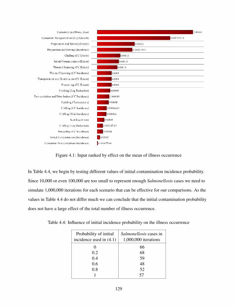
Figure 4.1: Input ranked by effect on the mean of illness occurrence

In Table 4.4, we begin by testing different values of initial contamination incidence probability.

Since 10,000 or even 100,000 are too small to represent enough Salmonellosis cases we need to

simulate 1,000,000 iterations for each scenario that can be effective for our comparisons. As the

values in Table 4.4 do not differ much we can conclude that the initial contamination probability

does not have a large effect of the total number of illness occurrence.

Table 4.4: Influence of initial incidence probability on the illness occurrence

Probability of initial Salmonellosis cases inincidence used in (4.1) 1,000,000 iterations

0 660.2 680.4 590.6 480.8 521 57

129

As discussed in Section 4.2.3.8, chlorine is used in the chilling pool to reduce the number of

Salmonella. A probability of 0.5 was used to model the skin contamination incident. However,

if this value varies, the total number of illness occurrence might change. Table 4.5 has the data

regarding different values for this probability. Based on the fact that the Salmonellosis cases’ val-

ues do not vary much, we can conclude that with the current log reduction of chlorine in (4.57),

the probability used in (4.56) does not affect the final illness occurrence tremendously.

Table 4.5: Influence of skin contamination incidence (4.56) on the illness occurrence

Probability of skin contamination Salmonellosis cases inincidence used in 4.56 1,000,000 iterations

0.0 860.25 630.50 680.75 531.0 31

Thorax cleaning, precooling, chilling, and transportation and distribution are the four stages be-

fore retail that are assumed to have potentials for CC. CC incidence rates are 0.2, 0.25, 0.2, and

0.25 for these stages, respectively. In Table 4.6, 4 multipliers (0.5, 1, 2, and 4), are tested to see

the influence of CC incidence rates. As shown in the table, the total illness occurrence values

does not increase by increasing the CC incidence rate. This indicates the low impact that these

values have on the final Salmonellosis cases.

Table 4.6: Influence of CC incidence probabilities on the illness occurrence

Ratio compared to original Probability of CC incidence in Salmonellosis cases invalues (0.2, 0.25, 0.2, 0.25) (4.38), (4.47), (4.58), (4.74) 1,000,000 iterations

0.5 0.1, 0.125, 0.1, 0.125 531 0.2, 0.25, 0.2, 0.25 682 0.4, 0.5, 0.4, 0.5 614 0.8, 1, 0.8, 1 58

Table 4.7 represents the illness numbers in 10,000 iteration for 5 different scenarios for the initial

contamination and CC extents’ parameters. By multiplying the mean and maximum of the CC

130

extent parameters by 5 different multipliers, we can see that the total illness occurrence changes.

The reduction from 68 to 28 indicates that if the average and maximum of the initial contami-

nation and CC extent get cut in half, the total number of Salmonellosis cases decreases by more

than 50%. Comparisons among all the values in Table 4.7 shows that the initial contamination

and CC extent have a great influence on the final number of illness occurrence.

Table 4.7: Influence of initial contamination and CC extent on the illness occurrence

Ratio compared to the original Initial contamination and CC extent parameters Salmonellosis cases inMPN values (0,1.5,2.5) (min, mean, max) in (4.2), (4.39), (4.48), (4.59), (4.75) 1,000,000 iterations

0.03 (0, 1, 2) CFU/chicken = (1,1,10) MPN/chicken 0

0.5 (0, 1.2, 2.2) CFU/chicken ≈ (1,15,150) MPN/chicken 28

1 (0, 1.5, 2.5) CFU/chicken ≈ (1,30,300) MPN/chicken 68

2 (0, 1.8, 2.8) CFU/chicken ≈ (1,60,600) MPN/chicken 408

3 (0, 2, 3) CFU/chicken = (1,100,1000) MPN/chicken 960

4.4 Conclusion and Future Work

This chapter details the creation of a Quantitative Risk Assessment Model (QRAM) that attempts

to assess the risk of Salmonellosis cases caused by contaminated chicken broiler produced in Chi-

nese companies. The work was done in collaboration with researchers in biological engineering,

poultry science, and numerous companies and universities throughout China.

To our knowledge, all the previous QRAMs regarding Salmonella in chicken, targeted for

human consumption, consider a pathway at retail and after it is purchased by a consumer, but our

model considered all the unit operations of the production and distribution. The QRAM is in-

formed by data collected from Chinese poultry producers since Fall 2016, published data, and

predictive models for growth/reduction of Salmonella at each stage. The model made use of

@Risk that is used to simulate 1,000,000 iterations representing 1,000,000 chickens and aimed to

estimate the final Salmonella extent in each chicken. The illness occurrence was then determined

by applying a dose-response model defined by Oscar (2004b).

131

Results shows that the number of Salmonellosis cases per 100,000 consumers is 1.70 which

is 4 times more than the value obtained in Oscar (2004b). Although, 95.6% of the Salmonellosis

cases are caused by consumers mishandling during the chicken preparation and serving, sensi-

tivity analysis demonstrated that by improving the production operations and the transportation

and distribution parameters regarding the extent of contamination, final number of Salmonellosis

cases can be reduced.

Furthermore, to evaluate the quality of the proposed model, a comparison between preva-

lence incidence of contaminated chickens at retail in our model and the real data derived from

samples taken from multiple supermarkets in 6 regions in China was performed. A close estimate

of the prevalence at retail was obtained, however, most of the input data regarding the extent of

contamination/cross-contamination are still required to be updated for a better risk assessment.

As the first step of the future study, we can name updating all the data regarding contam-

ination extent, CC incidence and extent for a better risk assessment. Also, new surveys repre-

senting Chinese consumers’ behavior and a specific DR model for Chinese people can assist the

model to better estimate the final Salmonellosis cases.

Although this model is designed specifically for the supply chain in Chinese companies,

it is flexible to model other supply chains as well. To this end, all the input data is required to be

specifically defined for the new pathway. Furthermore, this research is a good starting point for

developing a more comprehensive QRAM for Salmonella in chicken for a farm-to-fork pathway.

132

Bibliography

Bollaerts, K., Aerts, M., Faes, C., Grijspeerdt, K., Dewulf, J., and Mintiens, K. (2008). Humansalmonellosis: Estimation of dose-illness from outbreak data. Risk Analysis, 28(2):427–440.

Brown, M. H., Davies, K. W., BILLON, C. M.-P., Adair, C., and McCLURE, P. J. (1998). Quan-titative microbiological risk assessment: principles applied to determining the comparative riskof salmonellosis from chicken products. Journal of Food Protection, 61(11):1446–1453.

Bryan, F. L. and Doyle, M. P. (1995). Health risks and consequences of salmonella and campy-lobacter jejuni in raw poultry. Journal of Food Protection, 58(3):326–344.

Carol Beach (2016). Wal-Marts chicken safety program shows significant results.

Cassin, M. H., Lammerding, A. M., Todd, E. C., Ross, W., and McColl, R. S. (1998). Quantita-tive risk assessment for escherichia coli o157: H7 in ground beef hamburgers. Internationaljournal of food microbiology, 41(1):21–44.

CDC. Foodborne Diseases Active Surveillance Network (FoodNet) (2014). Foodnet surveillancereport for 2014 (final report). U.S. Department of Health and Human Services.

China National Center for Food Safety Risk Assessment (2015). Choose the chicken, pay atten-tion to health, prevention of Salmonella food poisoning.

Dickson, J. S. (1989). Enumeration of salmonellae by most-probable-number using thesalmonella 1–2 test. Journal of Food Protection, 52(6):388–391.

Holcomb, D. L., Smith, M. A., Ware, G. O., Hung, Y.-C., Brackett, R. E., and Doyle, M. P.(1999). Comparison of six dose-response models for use with food-borne pathogens. RiskAnalysis, 19(6):1091–1100.

Juneja, V. K., Melendres, M. V., Huang, L., Gumudavelli, V., Subbiah, J., and Thippareddi, H.(2007). Modeling the effect of temperature on growth of salmonella in chicken. Food microbi-ology, 24(4):328–335.

Lammerding, A. M. and Fazil, A. (2000). Hazard identification and exposure assessment formicrobial food safety risk assessment. International journal of food microbiology, 58(3):147–157.

Li, Y., Kidd, M., Kent, J., Raiwater, C., Liao, M., Ding, H., Ying, Y., Wang, M., and Qiao, X.(July 2016). Poultry excellence in china: In-field tests and risk assessment of salmonella con-tamination and fluoroquinolones residue for poultry supply chains. University of ArkansasTechnical Paper.

Mulder, N.-d. (2011). Crossroads for growth: The international poultry sector towards 2020.Utrecht: Rabobank.

133

Murphy, R., Duncan, L., Johnson, E., Davis, M., and Smith, J. (2002). Thermal inactivation d-and z-values of salmonella serotypes and listeria innocua in chicken patties, chicken tenders,franks, beef patties, and blended beef and turkey patties. Journal of food protection, 65(1):53–60.

Murphy, R., Marks, B., Johnson, E., and Johnson, M. (1999). Inactivation of salmonella andlisteria in ground chicken breast meat during thermal processing. Journal of Food Protection,62(9):980–985.

Nutrena (2017). Types of Poultry.

Oblinger, J. and Koburger, J. (1975). Understanding and teaching the most probable numbertechnique 1. Journal of Milk and Food technology, 38(9):540–545.

Oscar, T. (1998). The development of a risk assessment model for use in the poultry industry.Journal of food safety, 18(4):371–381.

Oscar, T. (2003). Comparison of predictive models for growth of parent and green fluorescentprotein–producing strains of salmonella. Journal of food protection, 66(2):200–207.

Oscar, T. (2004a). Dose-response model for 13 strains of salmonella. Risk Analysis, 24(1):41–49.

Oscar, T. (2006). Validation of a tertiary model for predicting variation of salmonella ty-phimurium dt104 (atcc 700408) growth from a low initial density on ground chicken breastmeat with a competitive microflora. Journal of food protection, 69(9):2048–2057.

Oscar, T. P. (2002). Development and validation of a tertiary simulation model for predicting thepotential growth of salmonella typhimurium on cooked chicken. International Journal of FoodMicrobiology, 76(3):177–190.

Oscar, T. P. (2004b). A quantitative risk assessment model for salmonella and whole chickens.International journal of food microbiology, 93(2):231–247.

Oscar, T. P. (2009). General regression neural network and monte carlo simulation model forsurvival and growth of salmonella on raw chicken skin as a function of serotype, temperature,and time for use in risk assessment. Journal of food protection, 72(10):2078–2087.

Oscar, T. P. (2011). Development and validation of a predictive microbiology model for survivaland growth of salmonella on chicken stored at 4 to 12 c. Journal of food protection, 74(2):279–284.

Palisade Corporation (2017). @RISK 5.x Tutorials.

Pan, C. (2013). Can chinas poultry move out of porks shadow. Still on the Road to Industrializa-tion,(Utrecht: Rabobank, 2013), 5.

Richard Lawley (2013). Salmonella.

134

Rosenquist, H., Nielsen, N. L., Sommer, H. M., Nørrung, B., and Christensen, B. B. (2003).Quantitative risk assessment of human campylobacteriosis associated with thermophiliccampylobacter species in chickens. International journal of food microbiology, 83(1):87–103.

Stopforth, J., Mai, T., Kottapalli, B., and Samadpour, M. (2008). Effect of acidified sodium chlo-rite, chlorine, and acidic electrolyzed water on escherichia coli o157: H7, salmonella, and liste-ria monocytogenes inoculated onto leafy greens. Journal of food protection, 71(3):625–628.

Surkiewics, B., Johnston, R., Moran, A., and GW, K. (1969). A bacteriological survey of chickeneviscerating plants. Food Technol, pages 80–85.

Teunis, P. F., Kasuga, F., Fazil, A., Ogden, I. D., Rotariu, O., and Strachan, N. J. (2010). Dose–response modeling of salmonella using outbreak data. International journal of food microbiol-ogy, 144(2):243–249.

United States Department of Agriculture Agricultural Research Service (2017). Growth factorsfor selected bateria.

Waldroup, A. (1996). Contamination of raw poultry with pathogens1. World’s Poultry ScienceJournal, 52(1):7–25.

Whiting, R. C. and Buchanan, R. L. (1997). Development of a quantitative risk assessment modelfor salmonella enteritidis in pasteurized liquid eggs. International Journal of Food Microbiol-ogy, 36(2-3):111–125.

Whittemore, A. (1993). Research note: a modified most probable number technique to enumeratetotal aerobes, enterobacteriaceae, and salmonella on poultry carcasses after the whole carcassrinse procedure. Poultry science, 72(12):2353–2357.

World Health Organization (2002). Risk assessments of Salmonella in eggs and broiler chickens,volume 2. Food & Agriculture Org.

World Health Organization (2003). Hazard characterization for pathogens in food and water:guidelines. Number 3. Food & Agriculture Org.

World Health Organization and others (2000). Overcoming antimicrobial resistance. Overcomingantimicrobial resistance.

Worldometers (2017). Countries in the world by population.

Yang, B., Qu, D., and Shen, Jinling, e. (2010). Resistance to salmonella and related genes infood-borne in shaanxi province. Journal of Biology, (6):788–796.

Zhijian, C. (2013). Shengnong development depth report: the amount of price increases, profitcycle reversed. Wuhan: Changjiang Securities, 3(38).

135

Appendix

4.A Quantitative Risk Assessment Model Information

Table 4.A.1: Quantitative Risk Assessment Model

Description Distribution/Formula

Initial ContaminationInput (incidence) iICin = Binomial(1,0.2)Input (extent) eIC

in = Pert(0,1.15,2.5)

Output (incidence) iICout = iICinOutput (extent) eIC

out = eICin ∗ iICin

SlaughteringInput (incidence) iSl

in = iICoutInput (extent) eSl

in = eICout

Input (temperature) Discrete({18,25,33},{0.25,0.5,0.25})Input (time) PERT (20,40,60)Input (extent log growth) d = 0

Output (incidence) iSlout = iSl

inOutput (extent) eSl

out = eSlin +d ∗ iSl

in

ScaldingInput (incidence) iSc

in = iSlout

Input (extent) eScin = eSl

outInput (temperature) t1 = PERT (50,57.5,65)Input (time) t2 = PERT (0.2,0.4,0.7)Input (extent log reduction) d = t2/10−0.1314∗t1+8.6599

Output (incidence) iScout = iSc

inOutput (extent) eSc

out = eScin −d ∗ iSc

in

Defeathering and RinsingInput (incidence) iDR

in = iScout

Input (extent) eDRin = eSc

outInput (temperature) t1 = PERT (10,15,20)Input (time) t2 = PERT (0.2,0.4,1)Input (extent log growth) d = 0

Output (incidence) iDRout = iDR

inOutput (extent) eDR

out = eDRin +d ∗ iDR

in

136

Table 4.A.2: Quantitative Risk Assessment Model (continued)

Description Distribution/Formula

EviscerationInput (incidence) iEv

in = iDRout

Input (extent) eEvin = eDR

outInput (temperature) t1 = PERT (10,15,20)Input (time) t2 = PERT (1,1.5,2)Input (extent log growth) d = 0

Output (incidence) iEvout = iEv

inOutput (extent) eEv

out = eEvin +d ∗ iEv

in

Thorax CleaningInput (incidence) iTC

in = iEvout

Input (extent) eTCin = eEv

outInput (temperature) t1 = PERT (5,10,15)Input (time) t2 = PERT (0.2,0.5,0.8)Input (extent log reduction) d = 0Input (CC incidence) iCC = Bernoulli(0.2)Input (CC extent) eCC = PERT (0,1.5,2.5)

Output (incidence) iTCout = max{iTC

in , iCC}Output (extent) eTC

out = iTCin ∗ (eTC

in −d)+(1− iTCin )∗ iCC ∗ eCC

PrecoolingInput (incidence) iPr

in = iTCout

Input (extent) ePrin = eTC

outInput (temperature) t1 = PERT (6,7,8)Input (time) t2 = PERT (5,7,10)Input (extent log reduction) d = 0Input (CC incidence) iCC = Bernoulli(0.2)Input (CC extent) eCC = PERT (0,1.5,2.5)

Output (incidence) iProut = max{iPr

in , iCC}Output (extent) ePr

out = iPrin ∗ (ePr

in −d)+(1− iPrin )∗ iCC ∗ eCC

137

Table 4.A.3: Quantitative Risk Assessment Model (continued)

Description Distribution/Formula

ChillingInput (incidence) iCh

in = iProut

Input (extent) eChin = ePr

outInput (temperature) t1 = PERT (0,1,2)Input (time) t2 = PERT (25,30,35)Input (chlorine density in ppm) ch =Uni f orm(20,70)Input (skin contamination incident) s = Bernoulli(0.5)Input (extent log reduction) d = PERT (0,0.3,2.1)Input (CC incidence) iCC = Bernoulli(0.2)Input (CC extent) eCC = PERT (0,1.5,2.5)

Output (incidence) iChout = max{iCh

in , iCC}Output (extent) eCh

out = iChin ∗ (eCh

in −d)+(1− iChin )∗ iCC ∗ eCC

StorageInput (incidence) iSt

in = iChout

Input (extent) eStin = eCh

outInput (temperature) t1 = PERT (−2,0,2)Input (time) t2 = PERT (60,600,2880)Input (extent log reduction) d = 0

Output (incidence) iStout = iSt

inOutput (extent) eSt

out = eStin−d ∗ iSt

in

Transportation and DistributionInput (incidence) iT D

in = iStout

Input (extent) eT Din = eSt

outInput (temperature) t1 = PERT (−2,0,2)Input (time) t2 = PERT (300,600,2880)Input (extent log reduction) d = 0Input (CC incidence) iCC = Bernoulli(0.25)Input (CC extent) eCC = PERT (0,1.5,2.5)

Output (incidence) iT Dout = max{iT D

in , iCC}Output (extent) eT D

out = iT Din ∗ (eT D

in −d)+(1− iT Din )∗ iCC ∗ eCC

138

Table 4.A.4: Quantitative Risk Assessment Model (continued)

Description Distribution/Formula

RetailRetail Input (incidence) iRe

in = iT Dout

Input (extent) eRein = iT D

out

Output (incidence) iReout = iRe

inOutput (extent) eRe

out = eRein

Consumer TransportationInput (incidence) iCT

in = iReout

Input (extent) eCTin = iRe

outInput (thermal abuse incidence) T = Bernoulli(0.02)Input (extent log growth) d = PERT (0.0005,0.04,0.15)

Output (incidence) iCTout = iCT

inOutput (extent) eCT

out = eCTin +d ∗T

CookingInput (incidence) iCo

in = iCTout

Input (extent) eCoin = iCT

outInput (extent log reduction) d = PERT (0.83,0.81,96)

Output (incidence) iCoout = iCo

inOutput (extent) eCo

out = eCoin −d

ServingInput (incidence) iSe

in = iCTout

Input (extent) eSein = eCT

outInput (CC incidence) iCC = Bernoulli(0.28)Input (CC extent rate) RCC = PERT (0.021,0.057,0.24)

Output (incidence) iSeout = max{iSe

in , iCC}Output (extent in MPN) eSe

out = iCC ∗b10eSein ∗RCCc+ b10eCT

outcConsumptionInput (incidence) iCin = 1, if eSe

out > 0, 0, otherwiseInput (extent) eC

in = eSeout

Input (Illness dose) D = 10PERT (0,3,7)

Output (Illness Occurrence) IO = 1 if eCin > D, 0 otherwise

139

4.B Certification of Student Work

140

5. Conclusion and Future Work

In this dissertation, three different security scenarios were modeled and solution methodologies

were proposed to address each problem. Chapter 2 presented a logic-based decomposition (LBD)

approach for a class of dynamic maximum flow network interdiction problems in which interdic-

tion activities must be scheduled in order to minimize the cumulative maximum flow over a finite

time horizon. The approach utilized a mixed integer formulation and a constraint programming

formulation to form our hybrid decomposition framework. Constraint programming was utilized

since it showed to be more efficient to formulate the scheduling aspects of the problem. LBD and

traditional mixed-integer programming approach got tested on various small and large instances

that were generated based on real data parameters and compared with each other. Computational

results suggested that LBD is more efficient in finding solutions for medium to large problem in-

stances when presolver if on and when presolver is off, LBD outperformed MIP for all size of

instances. In general it can be concluded that, LBD is comparable to MIP for smaller instances

but consistently outperform MIP for large instances.

One of the directions to which this work can be extended is to initialize LBD with a given

feasible solution. This solution can be generated by forcing LBD to just remove the first level

actors. While this chapter’s proposed approach offers better performance for solving large in-

stances, there remain applications for which even larger instances must be solved which makes

large-scale heuristics an appropriate avenue of study.

In Chapter 3, we introduced the Clustered Content Interdiction Problem (CCIP) which con-

siders groups of content dispersed across a collection of centers. In this problem, different con-

tent is assigned to the centers to ensure availability. Given a content assignment across a collec-

tion of available centers, an interdictor attempts to determine which centers to interdict in order

to minimize the content availability. An integer program P was formulated to model the problem,

which is proven to be NP-complete. Several modified formulations were developed by adding

symmetry breaking and other valid inequality constraints, and custom branchings to solve larger

problems more efficiently. They also exploit a genetic algorithm as a method to generate a quality

141

solution efficiently. The two best ones were selected for 100 S and M instances to be compared to

the original model P. The two models showed more efficiency for solving larger instances, how-

ever, the improvement is more for S instances.

For future study, a bilevel setting of the problem in cybersecurity context and also general-

izations of the matrix interdiction methodologies/approaches to allow for multiple content can be

explored.

In Chapter 4, we proposed a novel Quantitative Risk Assessment Model (QRAM) that at-

tempts to quantify the risk of microbial poultry contamination across the food supply chain in

China. This work was done in collaboration with biological engineering, poultry science and nu-

merous companies and universities throughout China. While all the previous QRAMs regarding

Salmonella in chicken, considered a pathway after it is purchased by a consumer, our model con-

sidered an extensive pathway in the supply chain that starts from the beginning of production

line and finishes by food consumption. It aimed to assess the risk of Salmonellosis human case

per 100,000 consumers. The model made use of @Risk that was used to simulate 1,000,000 it-

erations representing chickens. The illness occurrence was then determined by applying a does-

response model. Results showed that 1.70 cases of Salmonellosis occur in per 100,000 consumers

which can be reduced to less than 1. Analysis of the results indicated that 95.6% of the Salmonel-

losis cases are caused by consumers mishandling during the chicken preparation and serving.

However, sensitivity analysis demonstrated that by improving the production operations and the

transportation and distribution parameters regarding the extent of the contamination and cross-

contamination, final number of Salmonellosis cases can be noticeably reduced.

For future study we can incorporate lab-generated cross-contamination extent and inci-

dence data for an improved risk assessment. Furthermore, new surveys representing consumers’

behavior and a specific DR model for Chinese people can lead to a more precise model. This

model was designed specifically for the supply chain in Chinese companies, however, it is flex-

ible to model other supply chains. To achieve this goal, all the input data is required to be specifi-

cally defined for the new pathway. Furthermore, this research can be seen as a good starting point

142

for developing a more comprehensive QRAM for a farm-to-fork pathway.

143