modelling turbulent reactor flow using computational...

1 PVO

Modelling turbulent reactor flow using

Computational Fluid Dynamics

Polly Outram Trinity College

With

Szymon Leszczyński

Churchill College

Supervised by

Dr. Markus Kraft

PVO 2

Preface

The work described in this report is the result of my own research, unaided except as specifically

acknowledged in the text, and it does not contain material that has already been used to any

substantial extent for a comparable purpose. This report contains 42 pages.

I confirm that I have cleared the laboratory space I have used for the work described in this report,

to the satisfaction of my project supervisor. All chemical and biological samples have been

properly and safely disposed of according to University guidance.

Signed by Student __________________________________

Date __________________________________

I confirm that the student above has cleared the laboratory space used in this project to my

satisfaction.

Signed by Project Supervisor __________________________________

Date __________________________________

PVO 3

Summary

Systems involving turbulent reacting flow are prevalent and of considerable importance in

industry. This project aimed to gain further understanding of the use of Computational Fluid

Dynamics (CFD) for modelling the flow in such systems. A method for extracting Residence

Time Distributions (RTDs) from CFD, by injecting and tracking particles in a simulation, was

developed and used as a diagnostic tool to validate complicated CFD flow fields.

Results extracted from CFD simulations were successfully validated against analytic solutions for

laminar and turbulent pipe flow. Both velocity profiles and RTDs were compared, showing good

agreement with theory. The next stage in testing the method was to model a more complex system,

which was chosen to be the Cambridge Weblab reactor. RTDs were obtained for the Weblab

experimentally and compared with those extracted from a CFD simulation. CFD under predicts

the mean residence time of the Weblab reactor which could be because the mixing was due to

diffusion as well as forced convection, or the lack of internals in the simulation.

PVO 4

Contents

1 Introduction…………………………………………………… 5 2 Methods used………………………………………………….. 7 2.1 The Residence Time Distribution . . . . . . . . . . . . . . . . . . . 7 2.1.1 Obtaining CSTR RTDs from theory. . . . . . . . . . . . 7 2.1.2 Obtaining pipe RTDs from theory. . . . . . . . . . . . . 9 2.1.3 Obtaining RTDs from experiments. . . . . . . . . . . . . 9 2.2 Computational Fluid Dynamics . . . . . . . . . . . . . . . . . . . . 10 2.3 Extracting RTD from CFD. . . . . . . . . . . . . . . . . . . . . . . . 13 3 CFD Validation for Pipe Flow……………………………...... 17 3.1 Laminar pipe. . . . . . . . . . . . . . . . . . . . . . . . . . . . . . . . . . . 17 3.2 Turbulent pipe. . . . . . . . . . . . . . . . . . . . . . . . . . . . . . . . . . 21 3.3 Conclusions. . . . . . . . . . . . . . . . . . . . . . . . . . . . . . . . . . . . 25 4 The Weblab Reactor………………………………………….. 26 4.1 Background. . . . . . . . . . . . . . . . . . . . . . . . . . . . . . .. . . . . 26 4.2 Experimental Set up . . . . . . . . . . . . . . . . . . . . . . . . . 26 4.3 Calibration. . . . . . . . . . . . . . . . . . . . . . . . .. . . . . . . . . . . . 27 4.4 Experiments. . . . . . . . . . . . . . . . . . . . . . . .. . . . . . . . . . . . 28 4.5 Results. . . . . . . . . . . . . . . . . . . . . . . . .. . . . . . . . . . . . . . . . 31 5 Weblab: CFD vs. Experiment………………………………… 34 6 Conclusions and further work………………………………… 39 7 References……………………………………………………… 40 8 Acknowledgements…………………………………………….. 41 9 Nomenclature…………………………………………………... 41

1 INTRODUCTION

5 PVO

1 Introduction

Turbulent reactor flow and mixing is important in many industrial applications, from

pharmaceuticals and food processing to bioprocessing. It is used to prevent settling, increase heat

and mass transfer, ensure equal properties throughout a batch and create emulsions, (Aubin et al.,

2006). Turbulent flows also play a role in the ever increasing importance put on environmental

emissions, e.g. air pollution from incomplete combustion in an internal combustion engine, or by-

product formation in pharmaceutical industries, (Fox, 2003).

Analytical solutions can predict the mixing in an ideal stirred tank reactor, but to improve the

design of reactors an idea of the local non-idealities of specific systems is required. Observation

of fluid-flow in vessels is expensive and often hard, if not impossible, (Dong et al., 1993a).

Techniques such as laser doppler anemometry and particle image velocimetry can be used

experimentally to get a detailed three-dimensional view of the mixing characteristics in different

systems, but these methods are expensive and impractical for industrial design. They require

translucent reactor materials and contents, with very little gas hold-up so that light can pass

through the material and not be scattered. This is extremely unlikely in an industrial setting ,

(Aubin et al., 2006).

Computational Fluid Dynamics (CFD) is increasingly being used to design and optimise processes

in all areas of industry, (Joshi et al, 2003). Using CFD, flow regimes in reactors can be accurately

simulated to give a far more detailed view of local behaviour in a system and, as such, CFD can

produce results that cannot be gathered experimentally, (Santos et al., 2007). Optimisation of

systems by using accurate CFD modelling can increase productivity, corresponding to

substantially greater profit margins, (Harris et al., 1996). Particularly in turbulent mixing, the

wide range of mixing properties that different processes and materials require mean that design

involves an enormous number of variables. This is where CFD comes into its own, as modelling

has the advantage of easy parameter adjustment, (van Ertbruggen et al, 2007, Yapici et al, 2006).

1 INTRODUCTION

PVO 6

CFD codes implement a number of detailed physical models and use a range of sophisticated

numerical techniques which inherently need checking. This, combined with the fact that mixing

impellers produce complex flow-fields which are difficult to model, means simulations must be

validated against experimental results before they can be trusted. Currently experimental and CFD

results are mainly comparable qualitatively, (Farmer et al., 2005, Dong et al., 1993b). This project

develops and validates a method that provides a way of validating CFD simulations by extracting

CFD data that is directly and quantitatively comparable to experimental and theoretical data.

The validation method exploits Residence Time Distributions (RTDs), which are used

experimentally as a tool in diagnosing reactor problems and flow regimes. An RTD can be found

experimentally using tracer pulse experiments, and this can be compared to theoretical, ideal

RTDs. Some overall fluid flow problems can be identified from the differences between

experiment and theory, e.g., dead volumes or by-passing.

Our novel technique uses Lagrangian particle tracking in the CFD simulation to obtain RTDs. The

method is validated using two simple test cases which admit analytic solutions. It is then used to

validate the CFD flow-field in a complex system. Once validated, the simulation can be trusted as

accurate and the detail of the flow-field can be seen.

2 METHODS USED

7 PVO

2 Methods Used

Residence time distributions are at the crux of our method, and this section describes how RTDs

are obtained from experiment and theory. It goes on to describe the underlying principles of CFD,

and finally how RTDs are extracted from CFD-modelled solutions.

2.1 The Residence Time Distribution (RTD)

In a continuous reactor or vessel, elements of fluid will take different paths, resulting in a

distribution of times spent in the reactor. This distribution is called the exit age distribution, or the

Residence Time Distribution (RTD), E(t), and is normalised so that:

∫∞

=0

1dttE )( (1)

2.1.1 Obtaining Continuously Stirred Tank Reactor (CSTR) RTDs from theory

In a CSTR the normalised exit concentration gives the RTD:

∫∞=

0

dttc

tctE)(

)()( . (2)

In an ideal CSTR, the concentration in the exit stream is the same as in the whole reactor. The

concentration is:

⎥⎦⎤

⎢⎣⎡−=

τtctc exp)( 0 (3)

2 METHODS USED

PVO 8

and so the RTD becomes:

⎥⎦⎤

⎢⎣⎡−==

∫∞ ττ

t

dttc

tctE exp)(

)()( 1

0

(4)

where c is the tracer concentration and τ=V/Q is the mean residence time of the vessel, and where

Q is the flow out of the reactor and V is the reactor volume. Figure 1 shows the RTD predicted for

an ideal CSTR with τ = 535 seconds.

E(t) for Ideal CSTR τ =535

0

0.0002

0.0004

0.0006

0.0008

0.001

0.0012

0.0014

0.0016

0.0018

0.002

0 500 1000 1500 2000 2500

time (s)

E(t)

Figure 1: Graph to show an example of a theoretical CSTR RTD.

2 METHODS USED

PVO 9

2.1.2 Obtaining pipe RTD from theory

The residence time distribution of a pipe is obtained by using the velocity profile, u(r), and a

theoretical tracer pulse to calculate the cumulative distribution function of the tracer at the exit,

F(t). This is done by using q(r) i.e., volume arriving at the exit per second:

∫

∫== a

r

drrru

drrru

aqrqtF

0

0

2

2

)(

)(

)()()(

π

π. (5)

The RTD is then obtained by differentiating this cumulative distribution function with respect to

time:

dttdFtE )()( = . (6)

2.1.3 Obtaining RTDs from experiments

The RTD is determined experimentally by introducing a delta pulse of tracer at the inlet stream of

the continuous reactor and measuring the outlet concentration of the tracer. One way of measuring

concentration is by measuring the colour intensity in a system. This can be obtained using a

spectrophotometer, from which the concentration can be calculated using the Beer-Lambert Law:

( )clII ε−= exp0

(7)

where I is the intensity, I0 is the background intensity, c is the concentration, ε is the absorbance

and l is the path length in the spectrophotometer. ε l is a constant, which can be calculated

experimentally for the specific system, (§ 4.3). The normalised outlet concentration distribution is

then the RTD (equation (2)).

2 METHODS USED

PVO 10

2.2 Computational Fluid Dynamics (CFD)

Computational Fluid Dynamics (CFD) is a powerful tool that predicts the flow-field in a system.

Throughout this project the powerful commercial CFD code STAR-CD was used, which was

developed by CD-Adapco. This suite of tools consists of: StarDesign which is used for

unstructured mesh generation; Prostar, which was used to set up the physical models and

numerical methods, and for structured meshes; and Star, the actual solver. The steps involved in

setting up the simulations to model the flow are:

Draw a geometry using StarDesign;

Mesh the geometry, ensuring it is suitably refined in areas of particular interest;

Specify the physical properties of the fluids;

Set up pyhsical models, e.g., for turbulence;

Choose appropriate numerical methods for the transport equation;

Specify the boundary conditions.

The conservation of mass and momentum is then modelled in each of the cells using the Navier-

Stokes (NS) equations,

gUUUU ρυρρ +∇+−∇=∇⋅+∂∂ 2p

t (8)

together with the continuity equation,

0).( =∇+∂∂ Uρ

tp . (9)

In this report only systems which are both incompressible and isothermal are considered.

In turbulent systems, the velocity U(x,t) can be considered to be random, i.e., it will have a

different set of results for the same experiment done under the same flow conditions. Turbulent

flow is irregular, time-dependent and three-dimensional. However, the velocity is macroscopically

steady or “smooth” over time, i.e., it fluctuates around a steady mean value, (Deen, 1998). The

2 METHODS USED

PVO 11

governing equations (8) and (9) are complicated and non-linear. Reynolds-averaging the NS

equations leads to transport equations for the mean velocity, turbulent kinetic energy and turbulent

dissipation rate in high-Reynolds-number flows and with no reaction. These equations are

unclosed due to the Reynolds stress term. Various turbulence models seek to close these equations

by modelling this term. This is the so-called “turbulence closure problem”, (Fox, 2003).

The Reynolds-averaged Navier-Stokes (RANS) equation is:

ijii

ijjj

ij

i Uxx

px

uuxx

UU

tU

∂∂

+∂∂

−=∂∂

+∂

∂+

∂

∂ 21 υρ

. (10)

The unclosed term, ijuu , involves Reynolds stresses and can be modelled using the turbulent-

viscosity based model

⎟⎟

⎠

⎞

⎜⎜

⎝

⎛

∂

∂+

∂∂

+=i

j

j

iTijij x

UxU

kuu υδ32 (11)

where υT is the turbulent viscosity, which is given by:

ευ µ

2kCT = . (12)

The standard k-ε model is then:

)( 21 εεεσυεε

εεε

CCk

Ut

T −Ρ+⎟⎟⎠

⎞⎜⎜⎝

⎛∇⋅∇=∇⋅+

∂∂ (13)

where C ε 1, C ε 2, and σ ε are constants, given the standard values σ ε =1.3, C ε 1=1.44,

Cε 2=1.92, (CD Adapco group, 2004).

2 METHODS USED

PVO 12

These transport equations are solved together with the RANS equations in Prostar. It is also

necessary to define boundary conditions for these additional equations. This can be done either

by explicitly specifying values for k and ε, or alternatively by prescribing a turbulent intensity and

length scale. The latter approach was adopted, and the empirical relations used as follows:

81

060−

= Re.tI (14)

LLt 070.= (15)

where L is the characteristic length of the system under investigation, e.g., the diameter of the pipe,

(CD Adapco Group, 2004).

The k-ε High-Reynolds-Number model was used for all the turbulent simulations in this project. It

is a better turbulence model than Low-Reynolds-Number (LNR) model because this requires

integration all the way to the wall through the viscous sub-layer. This leads to numerical problems

and requires a far higher grid resolution, (Jones et al., 2001).

In order to establish the convergence of the solution, the global average residuals for a number of

key scalars were monitored. These included the three orthogonal momentum components,

pressure and the kinetic energy and dissipation rate of turbulence. Once all of these residuals fell

within a specified tolerance the solution was deemed to have converged. In these simulations a

residual tolerance of the order 1x10-8 was chosen, because it was found that this struck the correct

balance between accuracy of the solution and the computational time required to achieve it.

Finally, the converged solution was post-processed, to show the velocity and pressure fields in

each cell using coloured vectors or contours. Data can also be directly extracted for specified cells.

2 METHODS USED

PVO 13

2.3 Extracting RTD from CFD

To validate CFD simulations, data must be extracted from CFD that can be directly compared

with either experimental or analytical solutions. In this section, our novel method of extracting

RTDs from CFD is explained, along with how CFD was used to model various situations. An

overview of the process used is shown below (Figure 2).

Geometry drawn and meshed in Stardesign

Flowfield solved in Prostar

Lagrangian particles injected

and tracked

Gaussian smoothing to produce initial RTD

Compared to

theoretical RTD

Parameter optimised

Mesh refined

Figure 2: Schematic of the method used.

The required geometries were drawn and meshed using StarDesign. Three different mesh types

were used in the project: unstructured polyhedral, unstructured tetrahedral and structured

hexahedral. Figure 3 shows examples of these meshes.

Figure 3: (a) Polyhedral mesh (b) Tetrahedral mesh (c) Structured hexahedral mesh.

Generally speaking polyhedral meshes are more computationally efficient than tetrahedral (or

hexahedral) meshes. This is due to the fact that tetrahedral cells have only four faces, whereas the

polyhedral cells used in STAR typically have twelve-to-fourteen faces. This means that

2 METHODS USED

PVO 14

polyhedral cells have a greater number of neighbours and therefore communicate with more cells,

allowing the solution to propagate throughout the domain much more rapidly. Also,

although polyhedral cells have a greater number of faces, there will typically be fewer cells in total,

and therefore fewer faces overall in a poly mesh of a given domain. Therefore face-addressing

CFD solvers such as Prostar have fewer faces to loop over at each solution level, accelerating the

convergence speed, (CD Adapco Group, 2004). This was corroborated by our simulations, where

it was found that the polyhedral meshes typically converged. The size of the mesh can be refined

to give differing levels of detail, and more or less cells in specific areas.

The mesh was then imported into Prostar and the flow-field was solved using the methods

described in §2.2. Once converged to a global residual value of 1x10-8, Lagrangian particle

tracking was used with several different injection methods.

Our Lagrangian tracking routine was one-way coupled, so it was effectively a post-process. This

could be exploited in order to speed up the calculations by first obtaining a converged solution to

the continuous phase, and then freezing the flow-field (i.e., turning off the solver for all of the

continuous flow variables) before carrying out the dispersed phase calculations.

Groups of particles were injected at the inlet and tracked, and the time it took them to leave the

pipe was recorded. The injection methods were:

1. Circle – where one defines the number of circles, and the number of particles in each circle.

2. Planar – where one defines the plane size and position, and number of particles in grid.

3. Boundary – where one particle enters at every cell on the inlet face.

These are illustrated in figure 4.

2 METHODS USED

PVO 15

Figure 4: (a) Circle injection ( b) Planar injection (c) Boundary injection.

Circle and boundary injection methods mean that there is a higher number of particles injected

into the centre of the geometry, naturally biasing the exit-time distribution towards the faster

moving central areas. For this reason, it can be seen that a planar injection is the least biased

method, and therefore the strategy that was subsequently adopted.

The particles were tracked and the time it took for each particle to leave the pipe was extracted

from the CFD code. These data were converted into an RTD as follows:

Each discrete particle datum point, i, was smoothed using a Gaussian distribution:

( )2

2

1( ) exp22

ii

t tf t

σσ π

⎡ ⎤−= −⎢ ⎥

⎢ ⎥⎣ ⎦ (16)

where ti (the mean of the distribution) is the exit time of particle i, and σ2 (the variance) is an

adjustable parameter which efficiently serves as a filter width. The RTD was then constructed as

the superposition of all of these smoothed particles:

( )2

21 1

1( ) ( ) exp22

N Ni

ii i

t tE t f t

N σπσ= =

⎡ ⎤−= = −⎢ ⎥

⎢ ⎥⎣ ⎦∑ ∑ . (17)

This procedure was carried out using routines written in Matlab. The variance, σ2, is an adjustable

parameter, initially arbitrarily defined as 500, and then optimised with respect to the theoretical

2 METHODS USED

PVO 16

RTD. The optimisation was done using the least squares method to minimise the difference

between the theoretical and CFD results. For the case of the turbulent pipe and the reactor, the

parameter was optimised manually to obtain the best fit. Once the smoothed RTD was produced,

the mesh could be refined and the process repeated to optimise the fit between the predicted RTD

and the theory.

Imposing the Gaussian distribution onto discrete data results in tails that stretch infinitely

backwards and forwards in time. The effect of this is that a portion of the distribution is below the

minimum residence time of the reactor. Take, for example, a particle that travels at umax through

the system. This particle will emerge at tmin, but after smoothing, half of its Gaussian distribution

will be below tmin, which is physically impossible.

In the laminar pipe, the first particle to leave the pipe will be in the centre of the pipe, travelling

at:

avmax uu 2= . (18)

The minimum time to leave the pipe is then

τ50.min =t . (19)

For this reason, each individual particle distribution was truncated at 0.5τ. The area of the

remaining distribution was scaled up by the amount removed, to keep the area under the curve the

same. This was all carried out in the Matlab Gaussian filtering routine.

3 CFD VALIDATION FOR PIPE FLOW

17 PVO

3 CFD Validation for Pipe Flow

The first stage of testing the RTD validation method was to model a pipe in CFD and to

investigate whether the velocity profiles and RTDs obtained in this way agree with analytical

solutions.

3.1 Laminar Pipe

The first situation investigated was laminar flow in a pipe. A cylindrical pipe 1 m long and 1 m in

diameter was drawn in StarDesign. The average velocity was chosen to be 0.000089 ms-1 giving a

Reynolds number of 100. The pipe was meshed in Stardesign with a range of different mesh sizes

and the three mesh types. The meshes were imported into Prostar where the boundary conditions

and physical attributes of the model were defined. A parabolic laminar velocity profile was

prescribed across the inlet boundary. This was achieved by using a user-defined subroutine

written in Fortran.

The flow-field was solved with a maximum residual tolerance of 1x10-8. Figure 5 shows some

post-processed outputs of the velocity fields across the laminar pipe. The three different mesh

types showed similar results, all reproducing the expected parabolic laminar velocity profiles.

Figure 5: Polyhedral, tetrahedral and structured mesh post-processing for laminar flow in a pipe.


PVO 18

The flow-field was verified initially by comparing the theoretical velocity profile

⎟⎟⎠

⎞⎜⎜⎝

⎛−= 2

2

12aruru )( (20)

with the velocity profile obtained from the CFD calculation. Figure 6 shows the post-processed

velocity in a longitudinal cross section of the pipe. The velocity profile was extracted from Prostar

and is shown superimposed onto the theoretical profile.

Figure 6: (a) Axial cross-section of the CFD flow-field (b) Comparison of velocity profiles.

The converged flow-fields obtained for all the mesh types showed extremely good agreement with

theory. As the mesh size decreased (i.e., the number of cells increased), the solutions took longer

to converge but gave much smoother post-processing results.

Next, groups of 100 and 10000 particles were injected in the three different ways described in

§2.3 and were tracked through the pipe. The discrete data obtained (that is, the time taken to leave

the pipe) were recorded and were smoothed with a Gaussian filter as described in §2.3.

Theoretical velocity profile Velocity profile from CFD


PVO 19

The theoretical laminar RTD was calculated as follows.

⎟⎟⎠

⎞⎜⎜⎝

⎛−= 2

2

12aruru )( (21)

42

2

42

2

42

0

0 2

424

424

2

2

⎟⎠⎞

⎜⎝⎛−⎟

⎠⎞

⎜⎝⎛=

⎟⎟⎠

⎞⎜⎜⎝

⎛−

⎟⎟⎠

⎞⎜⎜⎝

⎛−

===

∫

∫ar

ar

aaau

arru

drrru

drrru

aqrqtF a

r

π

π

π

π

)(

)(

)()()( (22)

ttuL

ar

aru

tLu

21

21

12

2

2

2

2

τ−=−=⇒

⎟⎟⎠

⎞⎜⎜⎝

⎛−==

(23)

2

22

41

21

212

ttttF τττ

−=⎟⎠⎞

⎜⎝⎛ −−⎟

⎠⎞

⎜⎝⎛ −=)( (24)

3

2

2tdttdFtE τ==)()( (25)

The particles flowed along straight stream-lines in the pipe, as is characteristic of laminar flow.

Figure 7 shows the stream-lined particle tracks for 10 randomly selected droplets.

Figure 7: Particle tracks through the laminar pipe.


PVO 20

Results

The Gaussian-smoothed RTDs from the CFD simulations were compared to the analytical result.

Figure 8 shows the result of the simulation using a 5% polyhedral mesh with 10000 particles

injected, using the planar injection definition.

Laminar Pipe RTDs

0

0.0001

0.0002

0.0003

0.0004

0.5 1 1.5 2 2.5

t/tau

E(t)

CFD RTD

Theoretical RTD

Figure 8: Theoretical vs. Polyhedral mesh absolute sizing 5% 10000 particles, planar injection.

The CFD RTD shows good agreement with the theoretical RTD. It is fairly lumpy due to the

streamlined nature of the laminar flow-field, (figure 7). This meant that all the particles leaving

from the same injection point left the pipe at the same time in discrete groups. It was observed that

the mesh type and size made very little difference to the RTD. This is because all of the meshes

are sufficiently fine to resolve the flow-field. All the meshes adequately resolve the flow-field.

The polyhedral mesh was chosen because it is the most computationally efficient. The injection

definition made a big difference to the RTDs: with the circle and boundary definitions meant a lot

more particles were injected in the centre of the pipe than at the sides, which biased the final RTD.

The least biased injection definition was the planar injection. The number of particles injected had

the greatest effect on the final RTD. The number of particles must be large enough to give a

statistically representative distribution, with 10000 being sufficient.


PVO 21

3.2 Turbulent Pipe

The next situation modelled in order to test the validation method was a turbulent pipe. It was

drawn in StarDesign with length 30 m and diameter 0.5 m, which gives a Reynolds number of

112300. Meshes of varying sizes and types were created and imported into Prostar.

The boundary conditions applied were an inlet flow of 0.2 ms-1, in the direction normal to the inlet

plane. The entrance length was calculated using:

mLr

L

E

E

5.725.0*30

30

==⇒

≤ (26)

(Deen, 1998).

Therefore the flow was assumed to be fully turbulent after an entrance length of 10 m. Turbulent

intensity and length were calculated using equations (14) and (15) respectively.

0175.025.0*07.007.0014.0112300*06.0Re06.0 8

18

1

======

−−

LLI

t

t .

The flow-field was solved to a global residual of 1x10-8. Many problems were found when trying

to get a converged solution using a tetrahedral mesh. However, since the laminar case suggested

that mesh type had little effect on the RTD produced, this was not deemed a problem. Figure 9

shows the post-processed results across the pipe for the velocity field. It can be seen in figure 10

that the velocity profile is flatter in the centre of the pipe than in the laminar case, as expected.

Figure 9: Post processing results of turbulent flow, axial cross section.


PVO 22

The flow-field was initially validated by comparing the CFD produced velocity profile with the

analytic result. Turbulent velocity profiles are modelled empirically in several ways, including the

1/7th power law and the Von Karman velocity profile. All the empirical velocity profiles give very

similar results (Deen, 1998), so the Von Karman velocity profile was chosen for simplicity. The

velocity is calculated using the following equations:

Byuuu +⎟⎟⎠

⎞⎜⎜⎝

⎛=

υκ

** ln1 (27)

where B=5.5 is the Nikuradse constant, κ=0.4 is the Karman constant, υ=1.01x10-6 m2s-1 is the

kinematic viscosity, y [m] is the distance from the wall and u* is given by:

21

0⎟⎟⎠

⎞⎜⎜⎝

⎛=

ρτ*u (28)

where ρ=997.561 kgm-3 is the density and τ0 [Pa] is the wall shear stress:

2

2

0

ρυτ fC= (29)

where

25007910 .Re*. −=fC (30)

where µ=1.01x10-3 Pas is the viscosity.

The velocity profile across the pipe was extracted from Prostar and is shown with the theoretical

profile overlaid in figure 10.


PVO 23

Figure 10: Comparison of theoretical Von Karman and CFD velocity profiles.

The velocity profile resembles that predicted by the Von Karman velocity profile. The centre of

the pipe shows the largest disparity from theory, but this is probably due to the empirical nature of

the theoretical profile. The converged flow-fields obtained for all the mesh types showed good

agreement with theory.

As before, groups of 100 and 10000 particles were injected, tracked through the pipe, and the

discrete data obtained were recorded and smoothed with a Gaussian filter as described in §2.3.

The particles flowed in fairly straight lines but with slight deviation, as expected due to the

random fluctuations in turbulent pipe flow. Figure 11 shows the particle tracks for a few

randomly selected droplets.

Figure 11: Particle tracks in the turbulent pipe.


PVO 24

Results

The Gaussian smoothed RTD from CFD is compared to the analytical result in figure 12.

Turbulent Pipe RTDs

0

0.05

0.1

0.15

0.5 1 1.5 2 2.5

t/tau

E(t)

CFD RTD

Theoretical RTD

Figure 12: Theoretical vs. CFD Polyhedral mesh absolute sizing 5% 10000 particles.

The turbulent nature of the flow means that the CFD RTD is much smoother compared with that

of laminar flow, as there was no clumping of particles along streamlines. The RTD shows good

agreement with theory. Convergence problems with the tetrahedral mesh could not be overcome

by adjusting the mesh, the solving parameters or methods. Again, mesh-type and size had very

little effect upon the final RTDs. The injection method and number of particles had a far more

significant impact.

The theoretical RTD was calculated using the same method as shown in §3.1 equations (23)-(27),

substituting equation (23) with (33).


PVO 25

3.3 Conclusions

The method was successful in testing using laminar and turbulent pipe flow. Both the velocity

profiles and RTDs extracted from CFD showed good agreement with the analytic solutions.

The main conclusions drawn from this first stage of testing are:

all the meshes were fine enough to accurately solve the flow-field;

the polyhedral mesh was seen to be the most computationally efficient;

100 particles did not give a big enough sample size to produce a statistically representative

distribution, but 10,000 particles did;

the planar injection gave the least biased RTD.

The next stage of testing is to model a more complex system, the Weblab reactor, and test our

method by comparing the CFD results with those obtained from the experiments.

4 THE WEBLAB REACTOR

26 PVO

4 The Weblab reactor

4.1 Background

The final stage of our verification was to model a more complex system and compare an RTD from

CFD to one obtained experimentally. The Weblab reactor is of interest as it offers remote access to a

live experiment. The reactor is set up to perform colour change experiments, for example the reaction

of phenolphthalein in aqueous sodium hydroxide, and tracer experiments. For this project, only tracer

(Bengal Rose [0.001 M]) in water was used.

4.2 Experimental Set up

Figure 13 shows a simplified schematic of the Weblab, along with a detailed diagram of the reactor.

Inlet

Thermocouple

Non-Ideal Outlet

Stirrer

Outlet Figure 13: a) Schematic of Weblab reactor b) Detail of reactor.


PVO 27

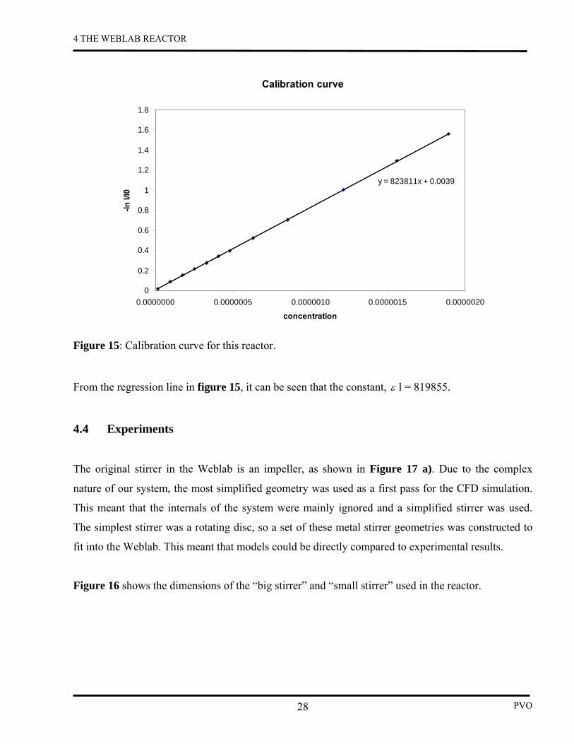
4.3 Calibration

The Beer-Lambert law was used to find the ε l constant for this system:

( )clII ε−= exp0

. (31)

Known volumes and concentrations of tracer were added to the reactor which was running in batch

mode. The concentration was therefore constant and calculable for each tracer dose. The volume of

water in the reactor was 249 ml. Figure 14 shows the intensity dropping with each tracer injection.

Intensity with increasing tracer concentration.

0

500

1000

1500

2000

2500

3000

3500

0 1000 2000 3000 4000 5000

Time (s)

Inte

nsity

Figure 14: Step tracer inputs showing decreasing intensity, i.e., increasing concentration.

These data were converted into a calibration graph using the following form of the Beer-Lambert

Law:

lcII ε=⎟⎟⎠

⎞⎜⎜⎝

⎛−

0

ln (32)

where I is the average Intensity at each “step”, and I0 is the background intensity.


PVO 28

Calibration curve

y = 823811x + 0.0039

0

0.2

0.4

0.6

0.8

1

1.2

1.4

1.6

1.8

0.0000000 0.0000005 0.0000010 0.0000015 0.0000020

concentration

-ln I/

I0

Figure 15: Calibration curve for this reactor.

From the regression line in figure 15, it can be seen that the constant, ε l = 819855.

4.4 Experiments

The original stirrer in the Weblab is an impeller, as shown in Figure 17 a). Due to the complex

nature of our system, the most simplified geometry was used as a first pass for the CFD simulation.

This meant that the internals of the system were mainly ignored and a simplified stirrer was used.

The simplest stirrer was a rotating disc, so a set of these metal stirrer geometries was constructed to

fit into the Weblab. This meant that models could be directly compared to experimental results.

Figure 16 shows the dimensions of the “big stirrer” and “small stirrer” used in the reactor.


PVO 29

Figure 16: Schematic of simplified stirrers.

Figure 17: The three stirrers used: a) Impeller b) “Big Stirrer” c) “Small Stirrer”.

Experiments were run using the ideal outlet at the base of the reactor and with a steady inflow of

water of 25 ml min-1. This was the maximum available flow rate. To ensure the mixing was only due

to the stirrer, not the dripping inlet, care was taken to make sure the water ran down the side of the

reactor rather than dripping in. The volume of water in the reactor was 260 ml and experiments were

run for the three different stirrers rotating at 240 rpm, and for no stirrer.

The tracer was injected into the system using the automated pulse injector at the top of the reactor.

This quite often froze up, so at the start of every experimental run the injector was tested. The

injection was exactly 1 ml of [0.001M] Bengal Rose.

Each experiment was started by carefully cleaning and filling the reactor with distilled water. The

volume was set using the arm on the side of the reactor, which had an exit to the drain. The water

inlet was started and set to its highest flow rate, and the system was observed until it reached steady

state. The tracer was injected at a recorded time and the colour intensity of fluid at the outlet was

observed and recorded.


PVO 30

Initially the spectrophotometer readings were taken approximately every 10 seconds and the intensity

was averaged over that time, giving large steps in the readings as shown in figure 18. This led to a

lack of fidelity in the most interesting and fast-moving early stages. This was overcome by modifying

the software used to take the readings, so that the intensity could be recorded at approximately 1

second intervals.

Initial intensity readings

0

500

1000

1500

2000

2500

3000

3500

4000

450 455 460 465 470 475 480 485 490 495 500

Time (t)

Inte

nsity

Figure 18: Graph to show the intensity readings before the apparatus was modified.

The reactor was left running and observed until the intensity had approximately regained its initial

level. Typically this took an hour.


PVO 31

4.5 Results

After the tracer was injected and mixed into the bulk water, a drop in the intensity was observed at

the outlet. The intensity gradually returned to its initial value as the tracer left the reactor in the outlet

stream. A measure of the speed of mixing can be made by examining the initial intensity drop, which

can be seen in figure 19.

Intensity with time

0

500

1000

1500

2000

2500

3000

3500

0 20 40 60 80 100

time (s)

Inte

nsity

Small Stirrer

No Stirrer

Impeller

Big Stirrer

Figure 19: Intensities of the outlet stream measure with time.

Figure 19 shows a close-up of the intensity data over the first 100 seconds. The system took

approximately 3000 seconds to return to its background intensity. The intensity measurements were

all time-rebased with respect to the tracer injection time. The graph shows that, as expected, the

impeller mixed the tracer into the reactor volume fastest indicated by the first drop in intensity. It also

stirred the tracer into the main volume most evenly, which can be seen by the smoothness of the

curve. The case with no stirrer gave the worst mixing properties, with the slowest intensity drop and

the least smooth curve. The peak in intensity at approximately 35 seconds is due to an area of high

concentration reaching the outlet, because the tracer had not been mixed well.


PVO 32

Counter-intuitively, the smaller stirrer shows a drop in intensity before the bigger stirrer. It is

expected that, since the mixing is a function of stirrer diameter, the bigger stirrer would mix better

than the smaller stirrer. This can be explained by the observation that the “big stirrer” blocks the path

of the tracer to the outlet due to its large diameter. This is apparent from the photographs of the

reactor shortly after tracer injection shown in figure 20. The “small stirrer” does not block the tracer

path and the tracer is mixed into the whole reactor volume evenly. The picture of the big stirrer

shows two distinct areas, above and below the stirrer, which are individually fairly well mixed but

have very different tracer concentrations

Figure 20: Pictures of the blocking by the large stirrer shortly after tracer impulse.

These intensities were converted into RTDs using the Beer-Lambert Law (equation (31) and equation

(2), §2.2.1).

Figure 21 shows the RTDs for the four separate experiments: impeller, “big stirrer”, “small stirrer”

and no stirrer.


PVO 33

Experimental RTDs

0

0.0002

0.0004

0.0006

0.0008

0.001

0.0012

0.0014

0.0016

0.0018

0 500 1000 1500 2000 2500

time

E(t)

ImpellerBig StirrerSmall StirrerNo Stirrer

Figure 21: RTDs of experimental runs.

Surprisingly, all of the runs, including the one with no stirrer present, gave similar RTDs. These

RTDs are all close to that predicted by theory, assuming the reactor is ideal, with τ=V/Q=535

seconds. Figure 22 shows the impeller and no stirrer cases are shown with the theoretical RTD, with

the impeller giving the closest result to the ideal theoretical line.

Theoretical vs Experimental RTDs

0

0.0002

0.0004

0.0006

0.0008

0.001

0.0012

0.0014

0.0016

0.0018

0.002

0 500 1000 1500 2000Time

E(t)

Impeller

No Stirrer

Theoretical

Figure 22: Experimental runs with theoretical RTD for Weblab (τ = 535 seconds) overlaid.

5 WEBLAB : CFD VS. EXPERIMENT

34 PVO

5 Weblab: CFD vs. Experiment

Once experimental RTDs had been obtained, the reactor could be modelled in CFD for the final stage

of validation. A simplified geometry of the reactor was drawn and meshed with a polyhedral mesh in

Stardesign. Most of the internal detail of the reactor was left out and only the simple stirrers were

modelled. An example of this geometry is shown below next to a detailed drawing of the reactor in

figure 23.

Figure 23: The simulation geometry and a schematic of the real reactor.

The reactor flow-field was solved using the following inlet boundary conditions: 1371 10*17.4min25 −−− = smml

Inlet diameter =0.0015 m, so uinlet = 0.224 ms-1.

The boundaries of the stirrer and rod were set to rotate at an angular velocity of 240 rpm. The flow-

field variables all converged to a global residual level of less than 1x10-8.


PVO 35

Figure 24 shows post-processed results which revealed flow patterns and swirl produced by the

stirrer, which were consistent with intuition and our observation (figure 20).

Figure 24: a) and b) Cross-sections length-ways through the reactor, showing velocity vectors.

Thermocouple

Non-ideal Outlet

Stirrer

InletCross sectionFigure 23 b)

Cross sectionFigure 23 a)

Figure 25: View of the reactor from above.


PVO 36

Figure 26: Flow-fields just above the stirrer. (a) is on the left and (b) is on the right.

Figures 27: Flow-fields around and below the stirrer. (c) is on the left and (d) is on the right.

Figures 26 and 27 show the flow patterns at various heights in the reactor.

Next, particles were injected into the inlet, which had been modelled as a pipe of diameter 2 mm at

the top of the reactor. The particles were specified to have the same properties as water and to

rebound if they hit the wall. 1500 particles making up 0.0045 kgs-1 were injected at the same

velocity as the fluid. They were injected at the inlet boundary at the top of the reactor, using the

planar injection method as described in §2.3, and were tracked through the pipe. The discrete data

obtained (that is, the time taken to leave the pipe) were recorded and smoothed with the Gaussian

filter, as described in §2.3.


PVO 37

The particles swirled around the reactor, with the fastest movement being directly around the

stirrer, as expected. This can be seen in figure 28 which shows the tracks of a few randomly

selected particles.

Figure 28: Particle tracks through the reactor.

It can be seen in figure 28 that, similarly to the experimental findings, the tracer gets “stuck”

above the “big stirrer”, spending a lot more time there than below the stirrer. This is an example of

a qualitative agreement with experimental results.

Figure 29 shows the RTD extracted from a “big stirrer” simulation, compared to the experimental

RTD.


PVO 38

Experimental vs CFD RTDs

0

0.002

0.004

0.006

0.008

0.01

0 500 1000 1500

time (s)

E(t)

CFD RTD

Experimental RTD

Figure 29: Graph to show experimental RTD compared to CFD RTD.

The CFD and experimental RTDs are quite different, with the τs being 140 seconds and 520

seconds respectively. This could result from mixing in the reactor arising from both diffusion and

forced-convection, where CFD only models forced convection. The model also does not include all

the internals, which could be barriers to mixing.

This disagreement shows the advantage of the RTD-validation method. Previously, qualitative

analysis of the CFD flow-field; the flow patterns seen in figures 24 to 28, and the observation of

tracer trapped above the stirrer seen in figures 20 and 27, would have led to the assumption that

the converged solution was sound. However, this new method allows the invaluable comparison of

the flow characteristics in the simulation and the real reactor, which shows that the simulation

must be improved before it can be trusted. The method allows for an iterative process of mesh

refining and increasing model detail increased until the RTDs produced are adequately similar.

6 CONCLUSIONS AND FURTHER WORK

39 PVO

6 Conclusions and further work

In this project a method of extracting RTDs from CFD was successfully developed. The method

involved freezing a converged CFD solution, and injecting and tracking particles through the

system. The discrete data extracted were Gaussian smoothed to produce the final RTD. The

method was used to produce CFD RTDs for laminar and turbulent pipe flow, both of which gave

good agreement with analytical solutions.

In the second stage of testing the method, a simulation of a real, complex system (the Weblab

reactor) was set up. RTDs for this system were extracted and compared to those found

experimentally. A set of simple stirrers was produced and used in the experiments, along with

the impeller that is used in standard Weblab runs. It was found that all of the RTDs produced

experimentally were similar to each other and similar to the theoretical, ideal RTD. This suggests

that either all of the stirrers had near ideal mixing properties, or that the majority of mixing took

place by methods other than forced convection. When comparing the experimental RTDs to

those extracted from CFD, it was found that CFD consistently underestimated the mean

residence time of the reactor.

This is extremely valuable information, showing that a purely qualitative comparison of

simulation and real-life can be misleading. In the situation studied the flow patterns suggested

that the simulation was accurate. The differences between CFD and experimental RTDs can be

used to improve the CFD simulation iteratively until an accurate solution is achieved. The

reasons behind differences can range from the model being overly simplified, meaning that dead

volumes from some of the internals blocking mixing have not been modelled, to the mesh

requiring refinment to give a more accurate representation of the swirl behaviour in the reactor.

Further work would take the Weblab model and improve the geometry, meshing and flow-field

solution of the CFD simulation until the RTD produced is comparable to that of the experiments.

The method could then be tested on other real-life situations to get a deeper understanding of the

requirements of an accurate CFD model.

7 REFERENCES

40 PVO

7 References

Aubin J., Fletcher D. F., Xuereb C. (2004). Modelling turbulent flow in stirred tanks with CFD: the influence of the modeling approach, turbulence model and numerical scheme. Experimental Thermal and Fluid Science. 28: 431-445. CD adapco Group. (2004). Star CD (version 3.22) User Guide. StarCDUserGuide.pdf: Software documentation. Deen W. M. (1998). Analysis of Transport Phenomena, 1. New York: Oxford University Press. Dong L., Johansen S. T., Engh T. A. (1993a). Flow Induced by an Impeller in an Unbaffled Tank-I. Experimental. Chemical Engineering Science. 49, 4: 549-560. Dong L., Johansen S. T., Engh T. A. (1993b). Flow Induced by an Impeller in an Unbaffled Tank-II. Numerical Methods. Chemical Engineering Science. 49, 20: 3511-3518. Duncan W. J., Thom A. S., Young A. D. (1970). Mechanics of Fluids, 2. Great Britain: Edward Arnold. Farmer R., Pike R., Cheng G. (2005). CFD analyses of complex flows. Computers and Chemical Engineering. 29: 2386-2403. Fox R. O., (2003). Computational Models for Turbulent Reacting Flows, 1. United Kingdom: University Press, Cambridge. Jones R. M., Harvey A. D., Acharya S. (2001). Two-Equation Turbulence Modeling for Impeller Stirred Tanks. Journals of Fluid Engineering. 123, 1: 640-648. Joshi, J. B., Ranade V. V., (2003). Computational fluid dynamics for designing process equipment: expectation, current status, and path forward. Industrial & Engineering Chemical Research. 42, 1115–1128. Kollman W. (1980). Computational Fluid Dynamics Volume 2, 1. US: Hemisphere Publishing Corporation. Harris C. K. et al. (1996). Computational Fluid Dynamics for Chemical Reaction Engineering. Chemical Engineering Science. 51, 10: 1569-1594. Perry R. H., Green D. W., Maloney J. O. (1984). The Chemical Engineers Handbook, 6th. New York: McGraw-Hill. Santos J. L. C., Geraldes V., Velizarov S., Crespo J. G. (2007). Investigation of flow patterns and mass transfer in membrane module channels filled with flow aligned spacers using computational fluid dynamics (CFD). Journal of Membrane Science. 305, 1: 103-117.

9 NOMENCLATURE

PVO 41

van Ertbruggen C., et al. (2007). Validation of CFD predictions of flow in a 3D alveolated bend with experimental data. Journal of Biomechanics, doi:10.1016/j.jbiomech.2007.08.013 Yapici K., Karasozen B., Schafer M., Uludag Y. (2006). Numerical Investigations of the effect of the Rushton type turbine design factors on agitated tank flow characteristics. Chemical Engineering and Processing. 10.1016. 8 Acknowledgements

My thanks go to Dr. Markus Kraft, Mr. Christopher Handscomb and Mr. Alastair Smith for their

continued guidance throughout this project. They, and most particularly Szymon Leszczynski, must

also be thanked for their kindness and patience through what has been an uncommonly challenging

year. Finally, my thanks go to Jack Rivett for proof reading, and to Sophie Smith for her unwavering

moral support.

9 Nomenclature B Nikuradse smooth walled pipe constant c Concentration Cε1 Constant Cε2 Constant Cµ Constant D Diameter F Cumulative distribution function I Intensity It Turbulent intensity k Turbulent kinetic energy l Length Lt Turbulent length LE Entrance length L Length p Pressure Q Flow rate r Radius t Time u Velocity ū Mean velocity

9 NOMENCLATURE

PVO 42

u* =(τ0/ρ)1/2 ׀v׀ Local average velocity

V Volume Greek Symbols є Molar absorbance ε Turbulent dissipation rate κ Karman constant σε Constant σ Parameter in Gaussian distribution η =yu*/ υ ρ Density φ =u/u* τ0 Wall shear stress τ Mean residence time µ Viscosity µG Mean in Gaussian distribution υT Turbulent viscosity υ Kinematic viscosity Subscripts Av Average G Gaussian Max Maximum T Turbulent Abbreviations CFD Computational Fluid Dynamics CSTR Continuously stirred tank reactor NS Navier-Stokes RTD Residence time distribution RANS Reynolds-averaged Navier Stokes

modelling turbulent reactor flow using computational...

Documents